Signal Detection Theory

A PRIMER OF

SIGNAL DETECTION THEORY

D. McNicolLecturer in Applied Psychology, University of New South Wales

LONDON. GEORGE ALLEN & UNWIN L.TDSYDNEY. AUSTRALASIAN PUBLISHING COMPANY

First published in 1972

This book is copyright under the Berne Convention. All rightsare reserved. Apart from any fair dealing for the purposes ofprivate study, research, criticism or review, as permittedunder the Copyright Act, 1956, no part of this publicationmay be reproduced, stored in a retrieval system, ortransmitted, in any form or by any means, electronic,electrical, chemical, mechanical, optical, photocopying,recording or otherwise, without the prior permission of thecopyright owner. Enquiries should be addressed to thepublishers.

© George Allen & Unwin Ltd 1972

British ISBN 0 04 152006 8 casedo 04 152007 6 paper

Australasian Publishing Company, Sydney SBN 900882 34 4

Prin ted in Great Britainin 10 on 12pt 'Monophoto' Times Mathematics Series 569by Page Bros (Norwich) Ltd., Norwich

Preface

There is hardly a field in psychology in which the effects of signaldetection theory have not been felt. The authoritative work on thesubject, Green's & Swets' Signal Detection Theory and Psychophysics (New York: Wiley) appearedjn 1966, and is having aprofound influence on method and theory in psychology. All thismakes things exciting but rather difficult for undergraduate studentsand their teachers, because a complete course in psychology nowrequires an understanding of the concepts of signal detection theory,and many undergraduates have done no mathematics at university 'level. Their total mathematical skills consist of dim recollections ofsecondary school algebra coupled with an introductory course instatistics taken in conjunction with their studies in psychology. Thisbook is intended to present the methods of signal detection theory toa person with such a mathematical background. It assumes a knowledge only of elementary algebra and elementary statistics. Symbolsand terminology are kept as close as possible to those of Green &Swets (1966) so that the eventual and hoped for transfer to a moreadvanced text will be accomplished as easily as possible.

The book is best considered as being divided into two mainsections, the first comprising Chapters 1 to 5, and the second,Chapters 6 to 8. The first section introduces the basic ideas ofdetection theory, and its fundamental measures. The aim is to enablethe reader to be able to understand and compute these measures.The section ends with a detailed working through of a typicalexperiment and a discussion of some of the problems which canarise for the potential user of detection theory.

The second section considers three more advanced topics. Thefirst of these, which is treated thoroughly elsewhere in the literature,is threshold theory. However, because this contender against signaldetection theory has been so ubiquitous in the literature of experimental psychology, and so powerful in its influence both in the

PREFACE

construction of theories and the design ofexperiments, it is discussedagain. The second topic concerns the extension of detection theory,which customarily requires experiments involving recognition tests,to experiments using more open-ended procedures, such as recall;and the third topic is an examination of Thurstonian scalingprocedures which extend signal detection theory in a number ofuseful ways.

An author needs the assistance of many people to produce hisbook, and I have been no exception. I am particularly beholden toDavid Ingleby, who, when he was working at the Medical ResearchCouncil Applied Psychology Unit, Cambridge, gave me much usefuladvice, and who was subsequently most generous in allowing me toread a number of his reports. The reader will notice frequentreference to his unpublished Ph.D. thesis from which I gainedconsiderable help when writing Chapters 7 and 8 of this book. Manyof my colleagues at Adelaide have helped me too, and I am gratefulto Ted Nettelbeck, Ron Penny and Maxine Shephard, who read andcommented on drafts of the manuscript, to Su Williams and BobWillson, who assisted with computer programming, and to myHead of Department, Professor A. T. Welford for his encouragement. I am equally indebted to those responsible for the productionof the final manuscript which was organised by Margaret Blaberably assisted by Judy Hallett. My thanks also to Sue Thom whoprepared the diagrams, and to my wife Kathie, who did the proofreading.

The impetus for this work came from a project on the applicationsof signal detection theory to the processing of verbal information,supported by Grant No A67/16714 from the Australian ResearchGrants Committee. I am also grateful to St John's College, Cambbridge, for making it possible to return to England during 1969 towork on the book, and to Adelaide University, which allowed me totake up the St John's offer.

A final word of thanks is due to some people who know moreabout the development of this book than anyone else. These arethe Psychology III students at Adelaide University who have servedas a tolerant but critical proving ground for the material whichfollows.

Adelaide University D. MCNICOL

September 1970

Contents

Preface

WHAT ARE STATISTICAL DECISIONS?

An exampleSome definitionsDecision rules and the criterionSignal detection theory and psychology

2 NON-PARAMETRIC MEASURES OF SENSITIVITY

The yes-no taskThe rating scale taskArea estimation with only a single pair of hit and false

alarm ratesThe forced-choice taskAn overall view of non-parametric sensitivity measures

3 GAUSSIAN DISTRIBUTIONS OF SIGNAL AND

NOISE WITH EQUAL VARIANCES

The ROC curve for the yes-no taskDouble-probability scalesThe formula for d'The criterionForced-choice tasks

4 GAUSSIAN DISTRIBUTIONS OF SIGNAL AND

NOISE WITH UNEQUAL VARIANCES

ROC curves for unequal variance casesSensitivity measures in the unequal variance caseMeasuring the signal distribution varianceThe measurement of response bias

5 CONDUCTING A RATING SCALE EXPERIMENT

Experimental design

page

1136

10

181825

3140 ~

45

505053575864

7980869192

99100

CONTENTS

Analysis of data 105Measures of sensitivity 113Measures of bias 119

6 CHOICE THEORY APPROXIMA TIONS TO

SIGNAL DETECTION THEOR Y 131The logistic distribution 134Determining detection measures from logistic distributions 136The matrix of relative response strengths 139Open-ended tasks 141A summary of the procedure for an open-ended task 147

Chapter 1

WHAT ARE STATISTICAL

DECISIONS?

AN EXAMPLE

70696865 66 67x = Height in inches

6463

Often we must make decisions on the basis of evidence which isless than perfect. F or instance, a group of people has heights rangingfrom 5 ft 3 in. to 5 ft 9 in. These heights are measured with the groupmembers standing in bare feet. When each person wears shoes hisheight is increased by 1 inch, so that the range of heights for thegroup becomes 5 ft 4in. to 5 ft 10 in. The distributions of heights formembers of the group with shoes on and with shoes off are illustratedin the histograms of Figure 1.1.

Solid line: Distribution 5 -shoes onDotted line: Distribution n-shoes off

- r - - --I

1 II II II 1

~ r---- - - - -I I

I 1

I I

I I

~ r - - -- - - - --I I

I I

I I

I I

r - - - - - - - - -I

I

II

I I

I I I I I II

o

4i6

3~ f6c~::::Jooo~ 2o i6~:.:::zo.0oet J..II 16~

185185186

157157162172180

219223225226229

239

206

215

7 THRESHOLD THEORY

Classical psychophysicsHigh threshold theory and the yes-no taskForced-choice tasksOther evidence favouring detection theory

8 THE LAWS OF CATEGORICAL AND

COMPARATIVE JUDGEMENT

Antecedents of signal detection theoryCategory rating tasksForced-choice tasks and the Law of Comparative

Judgement

Bibliography

Appendix 1 Answers to problems

Appendix 2 Logarithms

Appendix 3 Integration of the expression for the logistic curve

Appendix 4 Computer programmes for signal detection analysis

Appendix 5 Tables

Index

FIGURE 1.1

1

A PRIMER OF SIGNAL DETECTION THEORY

You can see that the two histograms are identical, with the exception that s, the 'Shoes on' histogram, is 1 in. further up the X-axisthan n, the 'Shoes off histogram.

Given these two distributions you are told that a particularperson is 5 ft 7 in. tall and from this evidence you must deducewhether the measurement was taken with shoes on or with shoes off.A look at these histograms in Figure 1.1 shows that you will not beable to make a decision which is certain to be correct. The histogramsreveal that 3/16ths of the group is 5 ft 7 in. tall with shoes off andthat 4/16ths of the group is 5 ft 7 in. tall with shoes on. The best betwould be to say that the subject had his shoes on when the measurement was taken. Furthermore, we can calculate the odds that thisdecision is correct. They will be (4/16)/(3/16), that is, 4/3 in favourof the subject having his shoes on.

You can see that with the evidence you have been given it is notpossible to make a completely confident decision one way or theother. The best decision possible is a statistical one based on theodds favouring the two possibilities, and that decision will onlyguarantee you being correct four out of every seven choices, on theaverage.

It is possible to calculate the odds that each of the eight heights

WHA TARE ST A TISTICAL DECISIONS?

of the group was obtained with shoes on. This is done in Table 1.1.The probabilities in columns 2 and 3 have been obtained from Figure1.1.

F or the sake of brevity we will refer to the two states of affairs'Shoes on' and 'Shoes off as states sand n respectively.

It can be seen that the odds favouring hypothesis s are calculatedin the following way:

For a particular height, which we will call x, we take the probability that it will occur with shoes on and divide it by the probabilitythat it will occur with shoes off. We could, had we wished, havecalculated the odds favouring hypothesis n rather than those favouring s, as has been done in Table 1.1.To do this we would have dividedcolumn 2 entries by column 3 entries and the values in column 4would then have been the reciprocals of those which appear in thetable.

Looking at the entries in column 4 you will see that as the value ofx increases the odds that hypothesis s is correct become more favourable. For heights of 67 in. andabove it is more likely that hypothesiss is correct. Below x == 67 in. hypothesis n is more likely to be correct.If you look at Figure 1.1 you will see that from 67 in. up, the histogram for 'Shoes on' lies above the histogram for 'Shoes off'. Below67 in. the 'Shoes off histogram is higher.

P{x I n) and P{x I s) are called 'conditional probabilities' and are the probabilitiesof x given n, and of x given s, respectively.

l(x) is the symbol for the 'odds' or likelihood ratio.

The evidence variableIn the example there were two relevant things that could happen.

These were state s (the subject had his shoes on) and state n (thesubject had his shoes off). To decide which of these had occurred, theobserver was given some evidence in the form of the height, x, ofthe subject. The task of the observer was to decide whether theevidence favoured hypothesis s or hypothesis n.

As you can see we denote evidence by the symbol x.' Thus x iscalled the evidence variable. In the example the values of x ranged

1 Another symbol used by Green & Swets (1966) for evidence is e.

SOME DEFINITIONS

With the above example in mind we will now introduce some ofthe terms and symbols used in signal detection theory.

o1/22/33/44/33/22/1

Odds favouring sl(x)

o1/162/163/164/163/162/161/16

Shoes on (s)p{xls)

._ L._

64656667686970

TABLE 1.1 The odds favouring the hypothesis 'Shoes on' for the eight possible heightsofgroup members.

--_._- - - - - - ---,---- - - - - -

----~rObabili~Of obt<li~ng~is height with _

Hi~~~~sin +Shoes off(n)x P{x\n)

--- -

63 1/162/163/164/163/162/161/16o

2 3

WHA TARE ST ATISTICAL DECISIONS?

H its, misses, false alarms and correct rejectionsWe now come to four conditional probabilities which will be

often referred to in the following chapters. They will be defined byreferring to Table 1.1.

First, however, let us adopt a convenient convention for denotingthe observer's decision.

The two possible stimulus events have been called sand n.Corresponding to them are two possible responses that an observermight make; observer says's occurred' and observer says 'n

occurred'. As we use the lower case letters sand n to refer to stimulusevents, we will use the upper case letters Sand N to designate thecorresponding response events. There are thus four combinationsof stimulus and response events. These along with their accompanying conditional probabilities are 'shown in Table 1.2.

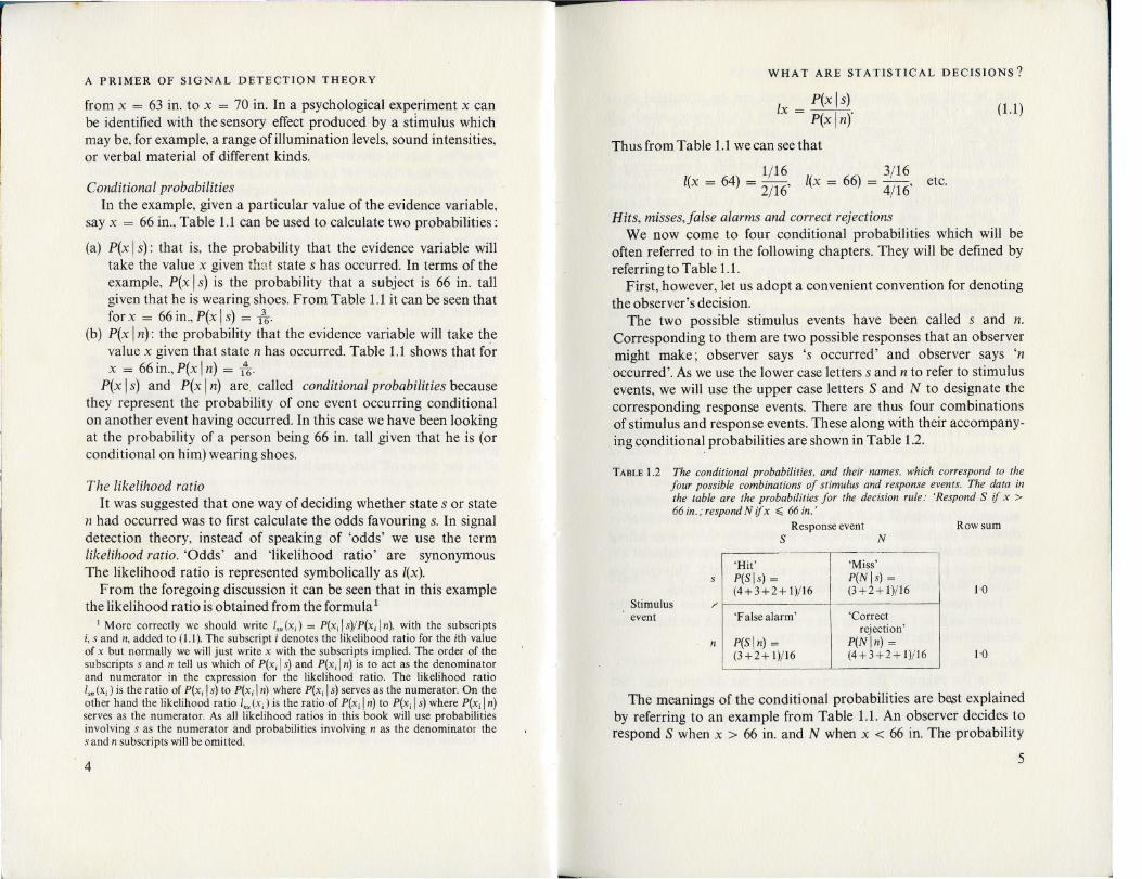
P(x Is)lx = P(xln)'

Thus from Table 1.1 we can see that


from x == 63 in. to x == 70 in. In a psychological experiment x canbe identified with the sensory effect produced by a stimulus whichmay be , for example, a range of illumination levels, sound intensities,or verbal material of different kinds.

Conditional probabilitiesIn the example, given a particular value of the evidence variable,

say x == 66 in., Table 1.1 can be used to calculate two probabilities:

(a) P(x Is): that is, the probability that the evidence variable willtake the value x given th at state s has occurred. In terms of theexample, P(x Is) is the probability that a subject is 66 in. tallgiven that he is wearing shoes. From Table 1.1 it can be seen thatfor x == 66 in., P(x Is) == 1

36'

(b) P(x In): the probability that the evidence variable will take thevalue x given that state n has occurred. Table 1.1 shows that forx == 66 in., Pix In) == 1

46'

P(x Is) and P(x I n) are, called conditional probabilities becausethey represent the probability of one event occurring conditionalon another event having occurred. In this case we have been lookingat the probability of a person being 66 in. tall given that he is (orconditional on him) wearing shoes.

1/16I(x = 64) = 2/16'

3/16I(x = 66) = 4/16' etc.

(1.1)

T he likelihood ratioIt was suggested that one way of deciding whether state s or state

n had occurred was to first calculate the odds favouring s. In signaldetection theory, instead of speaking of 'odds' we use the termlikelihood ratio. 'Odds' and 'likelihood ratio' are synonymousThe likelihood ratio is represented symbolically as l(x).

From the foregoing discussion it can be seen that in this examplethe likelihood ratio is obtained from the formula 1

1 More correctly we should write Isn(x j ) = P(xj Is)/P(xj !n), with the subscriptsi, s and n, added to (1.1). The subscript i denotes the likelihood ratio for the ith valueof x but normally we will just write x with the subscripts implied. The order of thesubscripts sand n tell us which of Pix, Is) and Pix, In) is to act as the denominatorand numerator in the expression for the likelihood ratio. The likelihood ratioIsn(x.] is the ratio of Pix, Is) to Pix, In) where Pix, Is) serves as the numerator. On theother hand the likelihood ratio Ins (Xi) is the ratio of Pix, In) to Pix, Is) where P(XjIn)serves as the numerator. As all likelihood ratios in this book will use probabilitiesinvolving s as the numerator and probabilities involving n as the denominator thes and n subscripts will be omitted.

4

TABLE 1.2 The conditional probabilities! and their names. which correspond to thefour possible combinations of stimulus and response events. The data inthe table are the probabilities for the decision rule: (Respond S if x >66 in.; respond N if x ~ 66 in. '

Response event Row sumS N

'Hit' 'Miss~

p(Sls) = p(Nls) =(4+3+2+1)/16 (3+2+1)/16

Stimulus /'

event 'False alarm 'Correctrejection'

n P(Sln) = P(Nln) =(3+2+1)/16 (4+ 3+ 2 + 1)! 16

The meanings of the conditional probabilities are best explainedby referring to an example from Table 1.1. An observer decides torespond S when x > 66 in. and N when x < 66 in. The probability

5

-A PRIMER OF SIGNAL DETECTION THEORY WHAT ARE ST A TIS TICAL DECISIONS?

TABLE 1.3 The number of correct and incorrect responses for /3=1 when P(s) =t P(n).

We can see how this rule works in practice by referring to theexample in Table 1.1.

Assume that in the example P(s) == ! P(n). Therefore by formula(1.2) [3 == 2 will be the criterion value of l(x) which will maximizecorrect responses. This criterion is twice as strict as the one which

If he says N when l(x) < 1 he will be correct 10 times out of 16,and incorrect 6 times out of 16. Ifhe says S when l(x) ~ 1 he.will becorrect 10 times out of 16, and incorrect 6 times out of 16. Overall, hischances of making a correct response will be 20/32 and his chancesof making an incorrect response will be 12/32.

Can the observer do better than this? Convince yourself that hecannot by selecting other decision rules and using Table 1.1 tocalculate the proportion of correct responses. For example, if theobserver adopts the rule: 'Say N if l(x) < i and say S if l(x) ~ i: his

, chances of making a correct decision will be 19/32, less than thosehe would have had with [3 == 1.

It is a mistake, however, to think that setting the criterion atf3 == 1 will always maximize the number of correct decisions. Thiswill only occur in the special case where an event of type s has thesame probability of occurrence as an event of type n, or, to put it insymbolic form, when P(s) = P(n). In our example, and in manypsychological experiments, this is the case.

When sand n have different probabilities of occurrence the valueof [3 which will maximize correct decisions can be found from theformula

Number of correct responses (out of48) = 10+(10x2) = 30Number of incorrect responses (out of48) = 6+(6x2) = 18

(1.2)

32

48

Total (out of48)16

Observer's responseS N

[3 == P(n)/P(s)

t =r- --- js 10 - 6

n __6 x 2 . __10 x_2 _Stimulus event

that he will say S given that s occurred can be calculated fromcolumn 3 of the table by summing all the P(x Is) values which fallin or above the category x == 66in., namely, (4+3+2+1)/16 ==

10/16. This is the value of P(S Is), the hit rate or hit probability. Alsofrom column 3 we see that P(N Is), the probability of responding Nwhen s occurred is (3+ 2 + 1)/16 '== 6/16. From column 2 P(N In), theprobability of responding N when n occurred, is 10/16, and P(S In),the false alarm rate, is 6/16. These hits, misses, false alarms andcorrect rejections are shown in Table 1.2.

DECISION RULES AND THE CRITERION

The meaning of [3In discussing the example it has been implied that the observer

should respond N if the value of the evidence variable is less than orequal to 66 in. If the height is greater than or equal to 67 in. he shouldrespond S. This is the observer's decision rule and we can state it interms of likelihood ratios in the following manner:

'If l(x) < 1, respond N; if l(x) ~ 1, respond S:

Check Table 1.1 to convince yourself that stating the decision rulein terms of likelihood ratios 'is equivalent to stating it in terms ofthe values of the evidence variable above and below which theobserver will respond S or N.

Another way of stating the decision rule is to say that the observerhas set his criterion at [3 == 1. In essence this means that the observerchooses a particular value of l(x) as his criterion. Any value fallingbelow this criterion value of l(x) is called N, while any value of l(x)equal to or greater than the criterion value is called S. This criterionvalue of the likelihood ratio is designated by the symbol [3.

Two questions can now be asked. First, what does setting thecriterion at [3 == 1 achieve for the observer? Second, are there otherdecision rules that the observer might have used?

Maximizing the number of correct responsesIf, in the example, the -observer chooses the decision rule: 'Set

the criterion at [3 == 1 in., he will make the maximum number ofcorrect responses for those distributions of sand n. This can bechecked from,Table 1.1 as follows:

6 7

B

•

(1.3)


maximized correct responses for equal probabilities of sand n.First we can calculate the proportion of correct responses whichwould be obtained if the criterion were maintained at f3 == 1. Thisis done in Table 1.3. As n events are twice as likely as s events, wemultiplyentries in row n of the table by 2.

The same thing can be done for f3 == 2. Table 1.1 shows thatf3 == 2 falls in the interval x == 69 in. so the observer's decision rulewill be: 'Respond S if x ~ 69 in., respond N if x < 69 in. Again,with the aid of Table 1.1, the proportion of correct and incorrectresponses can be calculated. This is done in Table 1.4.

WHAT ARE ST A TISTICAL DECISIONS?

(a) Maximizing gains and minimizinq losses. Rewards and penal-ties may be attached to certain types of response so that

~ S == value of making a hit,Cs N == cost of making a miss,C; S == cost of making a false alarm,v" N == value of making a correct rejection.

In the case where P(s) == P(n) the value of f3 which will maximizethe observer's gains and minimize his losses is

f3 = v"N + Cns.~s+ CsN

TABLE 1.4 The number of correct and incorrect responses for {3=2when P(s) =t P(n).

It can be seen that f3 == 2 gives a higher proportion of correctresponses than f3 == 1 when P(s) == t P(n). There is no other valueof f3 which will give a better result than 33/48 correct responses forthese distributions of sand n.

Other decision rulesOne or two other decision rules which might be used by observers

will now be pointed out. A reader who.wishes to see these discussedin more detail should consult Green & Swets (1966) pp. 20-7. Themain purpose here is to illustrate that there is no one correct value

.of l(x) that an observer should adopt as his criterion. The value off3 he should select will depend on the goal he has in mind and thisgoal may vary from situation to situation. For instance the observermay have either of the following aims.

8

Numberofcorrectresponses(outof48) = 3+(15x2) = 33Number of incorrect responses (out of 48) = 13 + (1 x 2) = 15

(1.4)

It is possible for a situation to occur where P(s) and P(n) are notequal and where different costs and rewards are attached to thefour combinations of stimuli and responses. In such a case the valueof the criterion which will give the greatest net gain can be calculatedcombining (1.2)with (1.3) so that

f3 = (v"N+ CnS) · P(n).(~s+CsN ). P(s)

9

It can be seen from (1.4)that if the costs of errors equal the values ofcorrect responses, the formula reduces to (1.2). On the other hand,if the probability of s equals the probability of n; the formula reducesto (1.3).

(b) Keeping false alarms at a minimun : Under some circumstances an observer may wish to avoild making mistakes of a particular kind. One such circumstance with which you will alreadybe familiar occurs in the conducting of statistical tests. The statistician has two hypotheses to consider; H 0 the null hypothesis, andHI' the experimental hypothesis. His job is to decide which of thesetwo to accept. The situation is quite like that of deciding betweenhypotheses nand s in the example we have been discussing.

In making his decision the statistician risks making one of twoerrors:

Type I error: accepting H 1 when H 0 was true, andType II error: accepting H 0 when H 1 was true.

32

48

Total (out of48)

1613

15 x 2

Observer's responseNs

3

lx2Stimulusevent : tL--_ I__


The Type I errors are analogous to false alarms and the Type IIerrors are analogous to misses . The normal procedure in hypothesistesting is to keep the proportion of Type I errors below some acceptable maximum. Thus we set up confidence limits of, say, p = 0·05,or , in other words, we set a criterion so that P(S In) does not exceed5 %. As you should now realize, by making the criterion stricter, notonly will false alarms become less'''11keiy but hits WIll also be decreased. In the language of hypothesis testing, Type I errors can beavoided only at the expense of increasing the likelihood of Type IIerrors.

SIGNAL DETECTION THEOR Y AND PSYCHOLOGY

The relevance of signal detection theory to psychology lies inthe fact that it is a theory about the ways in which choices are made.A good deal of psychology, perhaps most of it, is concerned with theproblems of choice. A learning experiment may require a rat tochoose one of two arms of a maze or a human subject may have toselect , from several nonsense-syllables, one which he has previouslylearned. Subjects are asked to choose, from a range of stimuli, theone which appears to be the largest, brightest or most pleasant.In attitude measurement people are asked to choose, from a numberof statements, those with which they agree or disagree. Referencessuch as Egan & Clarke (1966), Green & Swets (1966) and Swets(1964) give many applications of signal detection theory to choicebehaviour in a number of these areas.

Another interesting feature of signal detection theory, from apsychological point of view, is that it is concerned with decisionsbased on evidence which does not unequivocally support one out Qfa number of hypotheses. More often than not, real-life decisions have'to be made on the weight of the evidence and with some uncertainty,rather than on information which clearly supports one line of actionto the exclusion of all others. And, as will be seen, the sensoryevidence on which perceptual decisions are made can be equivocaltoo. Consequently some psychologists have found signal detectiontheory to be a useful conceptual model when trying to understandpsychological processes. For example, John (1967) has proposed atheory of simple reaction times based on signal detection theory;

10

WHA TARE ST A TISTICAL DECISIONS?

Welford (1968) suggests the extension of detection theory to absolutejudgement tasks where a subject is required to judge the magnitudeof stimuli lying on a single dimension ; Boneau, & Cole (1967) havedeveloped a model for decision-making in lower organisms andapplied it to colour discrimination in pigeons ; Suboski (1967) hasapplied detection theory in a model of classical discriminationconditioning.

The most immediate practical benefit of the theory, however,is that it provides a number of useful measures of performance indecision-making situations. It is with these that this book is concerned. Essentially the measures allow us to separate two aspectsof an observer 's decision. The first of these is called sensitivity, that is,how well the observer is able to make correct judgements and avoidincorr ect .ones. The second ofthese is called bias that is the exten tto which th;;observer favo~r~ one hypothesis ~ver an~ther independent of the evidence-h'e 'l ias been given. In the past these twoa'specfs " of~p'erfO'filiance have often ' been"confounded and this haslead to mistakes in interpreting behaviour.

Signal and noiseIn an auditory detection task such as that described by Egan,

Schulman & Greenberg (1959) an observer may be asked to identifythe presence or absence of a weak pure tone embedded in a burstof wh,itf! 1'!gise. (N oise, a hissing sound, consists of a wide band offrequencies of vibration whose intensities fluctuate randomly frommoment to moment. An everyday example of noise is the staticheard on a bad telephone line, which makes speech so difficultto understand.) On some trials in the experiment the observer ispresented with noise alone. On other trials he hears a mixture oftone + noise. We can use the already familiar symbols sand n torefer to these two stimulus events. The symbol n thus designates the~~e~t 'no ise alone ' and the symbol s designates the eyent 'signal (inthis case the tone) + noise '. '

. The selection of the 'appropriate response, S or N, by the observerraises the same problem of deciding whether a subject's height hadbeen measured with shoes on or off. A~s. _.!h.~ , nqj$~ beackground iscontinually fluctuating, some noise events are likely to be mistakenfor sig~al + noise events, and some signal + nois~. events will appear

11


to be like noise alone. On any given trial the observer's best decision'will again have to ' be '! sta~.is..!i9~1 one based on what he, .c9nsi~~~sare the odds that the sensory evidence favours s or n.

Visual detection tasks of a similar kind can also be conceived.The task of detecting the presence or absence of a weak flash oflight against a background whose level of illumination fluctuatesrandomly is one which would require observers to make decisionson the basis of imperfect evidence.

N or is it necessary to think of noise only in the restricted senseof being a genuinely random component to which a signal mayormay not be added. From a psychological point of view, noise mightbe any stimulus not designated as a signal, but whi,~h maybe ~0J1

fused with it. For example, we may be Interested in studying anobserver's ability to recognize letters of the alphabet which havebeen presented briefly in a visual display. The observer may havebeen told that the signals he is to detect are occurrences of the letter'X' but that sometimes the letters 'K'. 'Y' and 'N' will appearinstead. These three non-signal letters are not noise in the strictlystatistical sense in which white noise is defined, but they are capableof being confused with the signal letter, and, psychologically speaking, can be considered as noise.

Another example of this extended definition of noise may occurin the context of a memory experiment. A subject may be presentedwith the digit sequence '58932' and at some later time he is asked:'Did a "9" occur in the sequence?', or, alternatively: 'Did a "4"occur in the sequence?' In this experiment five digits out of a possible ten were presented to be remembered and there were fivedigits not presented. Thus we can think of the numbers 2,3,5,8, and9, as being signals and the numbers 1, 4, 6, 7, and 0, as being noise.(See Murdock (1968) for an example of this type of experiment.)

These two illustrations are examples of a phenomenon which,unfortunately, is very familiar to us-the fallibility of human perception and memory. Sometimes we 'see' the wrong thing or, inthe extreme case of hallucinations, 'see' things that are not presentat all. False alarms are not an unusual perceptual occurrence. We'hear' our name spoken when in fact it was not; a telephone canappear to ring if we are expecting an important call; mothers areprone to 'hear' their babies crying when they are peacefully asleep.

12


Perceptual errors '. may occur because o{ the Roor quality orambTgmty o{iii~ , stlmul~s"Rr,~s~nte~ to, a~ Qbserv~r~- 'The'lette; '-M'may be badly written so that it closely resembles an 'N'. The word'bat', spoken over a bad telephone line, may be masked to such anextent by static that it is indistinguishable from the word 'pat'. Butthis is not the entire explanation of the perceptual mistakes wecommit. Not only can the stimulus be noisy but noise can occurwithin the perceptual system itself. It is known that neurons in thecentral nervous system can fire spontaneously without externalstimulation. The twinkling spots of light seen when sitting in a dark"room are the result of spontaneously firing retinal cells and, ingeneral, the continuous activity of the brain provides a noisybackground from which the genuine effects of external signals mustbe discriminated (Pinneo, 1966). FitzHugh (1957) has measurednoise in the ganglion cells of cats, and also the effects of a signalwhich was a brief flash of light of near-threshold intensity. Theeffects of this internal noise can be seen even more clearly in olderpeople where degeneration of nerve cells has resulted in a relativelyhigher level of random neural activity which results in a corresponding impairment of some perceptual functions (Welford, 1958).Another example of internal noise of a rather different kind may befound in schizophrenic patients whose cognitive processes maskand distort information from the outside world causing failures ofperception or even hallucinations.

The concept of internal noise carries with it the implication thatall our choices are based on evidence which is to some extentunreliable (or noisy). Decisions in the face of uncertainty are therefore the rule rather the exception in human choice behaviour. Anexperimenter must expect his subjects to 'perceive' and 'remember'stimuli which did not occur (for the most extreme example of this seeGoldiamond & Hawkins, 1958). So, false alarms are endemic to anoisy perceptual system, a point not appreciated by earlier psychophysicists who, in their attempts to measure thresholds, discouragedtheir subjects from such 'false perceptions'. Similarly, in the studyof verbal behaviour, the employment of so-called 'corrections forchance guessing' was an attempt to remove the effects of falsealarms from a subject's performance score as if responses of thistype were somehow improper.

13

- --~-------_._~~------~--- - -


Problems

Before giving the pack to the subject the experimenter paints anextra spot on 225 cards as follows:

Number of cards inthis groupreceiving

an extra spot2550755025

Number of cardsin pack

5010015010050

12345

Number ofspotson card

1'2345

Original number ofspots on card

The subject is then asked to sort the cards in the pack into twopiles; one pile containing cards to which an extra spot has been addedand the other pile, of cards without the extra spot.

1. What is the maximum proportion of cards which can be sortedcorrectly into their appropriate piles?

2. State, in terms of x, the evidence variable, the decision rule whichwill achieve this aim.

3. If the subject stands to gain 1¢ for correctly identifying eachcard with an extra spot and to lose 2¢ for correctly classifying a'

15

The following experiment and its data are to be used for problems1 to 6.

In a card-sorting task a subject is given a pack of 450 cards, eachof which has had from 1 to 5 spots painted on it. The distributionof cards with different numbers of spots is as follows:


The fact is, if noise does playa role in human decision-making,false alarms are to be expected and should reveal as much about thedecision process as do correct detections. The following chapters of"this book will show that it is impossible to obtain good measures ofsensitivity and bias without obtaining estimates of both the hit andfalse alarm rates of an observer.

A second consequence of accepting the importance of internalnoise is that signal detection theory becomes something more thanjust another technique for the special problems of psychophysicists.All areas of psychology are concerned with the ways in which theinternal states of an individual affect his interpretation of information from the world around him. Motivational states, past learningexperiences, attitudes and pathological conditions may determinethe efficiency with which a person processes information and mayalso predispose him towards one type of response rather thananother. Thus the need for measures of sensitivity and response biasapplies over a wide range of psychological problems.

Egan (1958) was first to extend the use of detection theory beyondquestions mainly of interest to psychophysicists by applying it tothe study ofrecognition memory. Subsequently it has been employedin the study of human vigilance (Broadbent & Gregory, 1963a,1965; Mackworth & Taylor, 1963), attention (Broadbent & Gregory,1963b; Moray & O'Brien, 1967) and short-term memory (Banks,1970; Murdock, 1965; Lockhart & Murdock, 1970; Norman &Wickelgren, 1965; Wickelgren & Norman, 1966). The effects offamiliarity on perception and memory have been investigated bydetection theory methods by Allen & Garton (1968, 1969) Broadbent(1967) and Ingleby (1968). Price (1966) discusses the application ofdetection theory to personality, and Broadbent & Gregory (1967),Dandeliker & Dorfman (1969), Dorfman (1967) and Hardy &Legge (1968) have studied sensitivity and bias changes in perceptualdefence experiments.

N or has detection theory been restricted to the analysis of datafrom human observers. Suboski's (1967) analysis of discriminationcon~itioningin pig~?ns·'li-~·~-·alreaaY'-fie¢n . tTIentio~ed, ' and C Nevin(1'965) and Riflirig~" '& " ~Mcvb'l~imid (i965) ' ''hav~" ' '' ~i so .studied dis-crimination iii ' '' pIge6ilff ''by'~ ~d'ete'(;ti6h+ e theory methods. Rats have(~G.eiYed_s.imilar · a,tJe!!!i.Qn.IiQn1 ~.B.~c;k .f!9~}I, ~l}g. "NeYi·~"!1964):'-..

14

16


17

(a) for the problem data,(b) for the data in Table 1.1.

(The issues raised in this problem will be discussed in Chapter 4.)

~.. "

40'60'9

30'50'8

x 1P(x In) 0'2P(x Is) 0'5

8. At a particular value of x, l(x) = 0'5 and the probability of xgiven that n has occurred is 0'3. What is the probability of x giventhat s has occurred?


card as containing an extra spot, find firstly in terms of f3~ andsecondly in terms of x, the decision rule which will maximize hisgains and minimize his losses.

4. What proportions of hits and false alarms will the observerachieve ifhe adopts the decision rule f3 = f?5. What will P(N Is) and f3 be if the subject decides not to allow thefalse alarm probability to exceed i?

6. If the experimenter changes the pack so that there are two cardsin each group with an extra spot to every one without, state thedecision rule both.in terms of x and in terms of f3 which will maximizethe proportion of correct responses.

7. Find the likelihood ratio for each value of x for the followingdata:

9. If P(S Is) = 0'7 and P(N In) = 0'4~ what is P(N Is) and P(S In)?

10. The following table shows P(x In) and P(x Is) for a range ofvalues ofx.

x 63 64 65 66 67 68 69 70 71P(x In) 1/16 2/16 3/16 4/16 3/16 2/16 1/16 0 0p(x 'i s) 1/16 1/16 2/16 2/16 4/16 2/16 2/16 1/16 1/16

Draw histograms for the distributions of signal and noise andcompare your diagram with Figure 1.1. What differences can yousee?Find l(x) for each x value in the table. Plot l(x) against x for yourdata and compare it with a plot of l(x) against x for the data inTable 1.1. How do the two plots differ?If P(s)were equal to 0'6 and P(n) to 0'4 state, in terms of x, the decisionrule which would maximize correct responses:


12'

< 5.

~ x ~ 66.

1. f3

Lax0'900'70

Medium0'700'30

Strict0'500'14

1. Criterion:P(S Is)P(SIn)

(a) 0'74.2. (a) Observer 1 :

P(S Is) = 0'31,0'50,0'69,0'77,0'93,0'98, 1'00.P(SIn) = 0'02,0'07,0'16,0'23, 0'50, 0~69, 1'00.Observer 2:P(S Is) = 0'23,0'44,0'50,0'60,0'69,0-91, 1'00.p(SI n) == 0'11,0'26,0'31,0'40,0'50,0-80,1.'00.

(b) Observer 1. = 0'85; observer 2 = 0'63.

CHAPTER 2

CHAPTER

Appendix 1

1. 0'67.2. RespondSwhenx ~ 4; respond N when x ~ 3.3. f3 = 2. Respond S when x ~ 5 ; respond N when x4. p(S Is) = 0'67, P(S In) = 0'33.5. P(N\s) = 0'11 ;f3 = ~or~.

6. Respond S when x ~ 2; respond N when x7. l(x) = 2'50, 1'75, 1'60, 1'50.8. p(xIS) = 0'15.9. P(N Is) = 0'3, P(SIn) = 0'6.

10. l(x) = 1,1, j ,1,1,1,2, 00, 00. .

(a) Respond S if x ~ 63 or if x ~ 67. Respond N If 64(b) Respond S ifx ~ 65; respond N if x < 65.

ANSWERS TO PROBLEMS

SAFFIR, M. A. ( 1937), 'A comparative study of scales constructed by three psychophysical methods', ~sychometrika, 2,179-98.

SCHONEMANN, P. H. , & TUCKER, L. R. (1967) , 'A maximum likelihood solution forthe method of successive intervals allowing for unequal stimulus dispersions',Psychometrika, 32, 403-17.

SCHULMAN, A. 1., & MITCHELL, R. R. (1966), 'Operating characteristics from yes-noand forced-choice procedures', J. acoust. Soc. Amer. , 40, 473-7.

SJOBERG, L. (1967) , 'Successive intervals scaling of paired comparisons' , Psychometrika. 32, 297-308.

STOWE, A. N., HARRIS, W. P., & HAMPTON, D. B. (1963) , 'Signal and context components of word recognition behaviour', J. acoust. Soc. Amer. , 35, 639-44.

SUBOSKI, M. D. (1967), 'The analysis of classical discrimination conditioning experiments ', Psychological Bulletin, 68, 235-42 ~

SWETS, 1. A. (1959) , 'Indices of signal detectability obtained with various psychophysical procedures' , J. acoust. Soc. Amer. , 31,511-13 .

SWETS, J. A. (1961) , 'Is there a sensory threshold 7', Science. 134, 168-77.SWETS, J . A. (Ed.) (1964) , Signal detection and recognition by human observers. New

York: Wiley.

SWETS, J. A., TANNER, W. P. JR., & BIRDSALL, T. G. (1961) , 'D ecision processes inperception', Psychological Review , 68, 301--40.

SYMONDS, P. M. (1924) , 'On the loss in reliability in ratings due to coarseness of thescale', Journal ofExperimental Psychology, 7, 456-61.

TANNER, W. P. JR. (1961) , 'Physiological implications of psychophysical data' ,Science,89, 752-65.

TEGHTSOONIAN, R. (1965) , 'The influence of number of alternatives on learning and, performance in a recognition task ', Canadian Journal of Psychology, 19. 31-41.THORNDIKE, E. L. , & LORGE, I. (1944) , The teacher's word book of 30.000 words,

New York: Teachers College, Columbia University, Bureau of Publications.THURSTONE, L. L. (1927a), 'Psychophysical analysis ', Am erican Journal ofPsychology.

38,368-89.

THURSTONE, L. L. (1927b), 'A Law of Comparative Judgement', PsychologicalReview, 34, 273-86.

TIPPETT, L. H. C. (1925) , 'On the extreme individuals and the range of samples takenfrom a normal population', Biometrika, 17, 364-87.

TORGERSON, W. S. (1958), Theory and methods ofscaling, New York: Wiley.TREISMAN, M. , & WATTS, T. R. (1966), ' R ela tion between signal detectability theory

and the traditional procedures for measuring sensory thresholds: estimating d'from results given by the method of constant stimuli', Psychological Bulletin , 66,438-54.

WATSON, C. S., RILLING,M. E. , & BOURBON, W. T. (1964) , 'Receiver-operatingcharacteristics determined by a mechanical analog to the rating scale', J. acoust.Soc. Amer. ,36, 283-8 .

WELFORD, A. T . (1968) , Fundamentals of skill, London: Methuen.WELFORD, A. T. (1958) , Ageing and human skill, Oxford: Oxford University Press.WICKELGREN, W. A. (1968) , 'Unidimensional strength theory and component

analysis of noise in absolute and comparative judgements ', J. math. Psychol.. 5,102-22.

WICKELGREN, W. A. , & NORMAN, D. A. (1966) , 'Strength models and serial positionin short-term recognition memory', J. math. Psychol. , 3,316-47.

219218

Signal Detection Theory

Documents

Transcript of Signal Detection Theory