Short-time FFT based laser Doppler velocimetry for bubbly...

18th International Symposium on the Application of Laser and Imaging Techniques to Fluid Mechanics・LISBON | PORTUGAL ・JULY 4 – 7, 2016

Short-time FFT based laser Doppler velocimetry for bubbly two-phase turbulent boundary layers

H. J. Park1,* , K. Toda2, Y. Oishi3, Y. Tasaka1, Y. Murai1

1: Faculty of Engineering, Hokkaido University, Japan 2: Graduate School of Engineering, Hokkaido University, Japan

3: College of Design and Manufacturing Technology, Muroran Institute of Technology, Japan * Correspondent author: [email protected]

Keywords: Laser Doppler Velocimetry, Bubble, Turbulent Boundary Layer

ABSTRACT

Bubbly drag reduction (BDR) technique has been recently applied to low speed vessels for actual use. Despite to

applications on progress, we do not clearly understand microscopic mechanisms hidden complicatedly in BDR. Here,

we focus velocity distribution in a turbulent boundary layer, especially a viscous sublayer, because wall shear stress

is directly evaluated from velocity profiles in this layer. To investigate velocity modification by bubbles injected into

the boundary layer, we developed a laser Doppler velocimetry (LDV) with a high spatial resolution enough to access

the layer. A data processing using a short-time FFT analysis and a statistical analysis was devised to calculate

velocities automatically from beat signals including low frequency noises generated by an inverter in experimental

facility. Velocity distributions with a single-phase flow and a two-phase flow were investigated by the LDV with the

data processing, and were evaluated using statistical values, such as average, standard deviation, skewness and

kurtosis. By these analyses, it is confirmed that the bubbles have a big potential to modify characteristics of the

velocities even with a low void fraction.

1. Introduction

Bubbles injected into a turbulent boundary layer modify completely its characteristics. For

example, they are possible to reduce wall friction on a turbulent boundary layer and the maximum

drag reduction rate by bubble injection is up to 80% [1]. Since bubbly drag reduction (BDR)

reported by McCormick and Bhattacharyya [2], it has researched to improve energy efficiency of

sailing large vessels by reducing frictional drag occupying approximately 80% of total drag of the

vessels. Although many researches on BDR have been performed for over 40 years, we do not

clearly understand this phenomenon yet. Ceccio [3] reviewed many previous researches on BDR

and summarized a relationship between BDR rate and void fraction. According to this review

article, variance of the rate has a trend that basically it becomes larger as the void fraction increases.

When the void fraction is lower than a critical void fraction, however, frictional drag is increased

by adding bubbles. Although this trend appears at the all previous researches summarized in


Ceccio [3], the BDR rate is not summarized by the void fraction because it is greatly affected by

experimental conditions and facilities. Also, Murai [4] summarized effects by adding bubbles in

flows and their conduciveness on the drag reduction at his review paper and made a map of main

effect of bubbles according to a flow speed and a bubble size. Unfortunately, this transition map

is not perfect because the effect and its conduciveness are influenced by other factors such as void

fraction [3], wall roughness [5] and entrance distance from a bubble injector [6, 7]. Summarizing

these, BDR is affected by several factors associated with flows and investigation of effects of the

bubbles with considering these all factors is required to understand BDR. Unfortunately, it is

actually impossible to grasp influences of the all factors. Besides, even if we have clear information

of each factor, it is hard to understand BDR because of a non-linearity occurring by mutual

interactions between the factors.

For deeper understanding of BDR, as the first step, we focus modification of velocity

distribution in a turbulent boundary layer, especially a viscous sublayer, by bubble injection

because a velocity gradient in the viscous sublayer is linked directly with wall shear stress (τw),

which is defined as

𝜏w = 𝜌𝜈 |𝑑𝑢

𝑑𝑦|𝑦=0

. (1)

Here, ρ, ν, u and y are density of fluid, viscosity of fluid, velocity and depth from the wall.

Assuming that ρ and ν in the viscous sublayer are not changed by the bubbles because thin liquid

film exists between the bubbles and the wall [8], the velocity gradient has to be decreased by the

bubbles when BDR occurs. Modification of the velocity gradient means that turbulent flow

structures are changed by the bubbles. To achieve our purpose, we designed a laser Doppler

velocimetry with a high spatial resolution to access the turbulent boundary layer without any

interference on velocity distribution by measurement instrument and estimated effects of the

bubbles on the turbulent boundary layer by investigating velocity fluctuation in the layer.

2. Experimental facilities and conditions

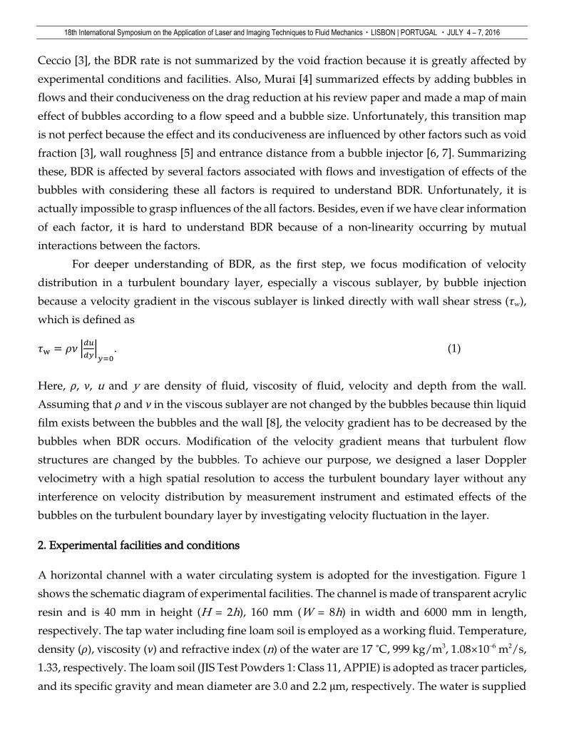
A horizontal channel with a water circulating system is adopted for the investigation. Figure 1

shows the schematic diagram of experimental facilities. The channel is made of transparent acrylic

resin and is 40 mm in height (H = 2h), 160 mm (W = 8h) in width and 6000 mm in length,

respectively. The tap water including fine loam soil is employed as a working fluid. Temperature,

density (ρ), viscosity (ν) and refractive index (n) of the water are 17 °C, 999 kg/m3, 1.08×10–6 m2/s,

1.33, respectively. The loam soil (JIS Test Powders 1: Class 11, APPIE) is adopted as tracer particles,

and its specific gravity and mean diameter are 3.0 and 2.2 μm, respectively. The water is supplied


to the channel by a pump and its liquid flowrate (Q) is measured by a flowmeter. To inject bubbles

into the channel, a syringe is installed on the upper wall of the channel at x/h = 64 and z/h = 1.5.

Here, x, y, and z directions are defined to be the streamwise, vertical and spanwise directions. The

origin of the coordinate system corresponds to inlet, upper wall and nearside wall of the channel.

Injected bubbles are removed in a water tank located at the end of the channel and only the water

is circulated to the channel. As seen in the figure, a camera and a laser Doppler velocimetry system,

which is composed by a laser source and an optical receiver, is located at x/h = 70 for the

investigation. The laser source is tilted away towards the upper wall with 4° and emits two laser

beam having 655 nm in wavelength (λ) with a crossing angle (θ = 16°). The beams are crossed at

z/h = 1.5, reflected at the upper wall, and finally reached to the optical receiver. Interference

fringes to make beat signal for measuring a flow velocity are formed in the beam crossing area

with 19 μm in the vertical direction, 19 μm in the streamwise direction and 150 μm in the spanwise

direction. The optical receiver converts a variance of laser beam to an electronical signal and send

it to a data logger (NR-500, KEYENCE) connected to the receiver. The data logger has 1 MHz in a

temporal resolution and record the signal for 2.5 s. The laser source and the optical receiver are

moved by traversers which are possible to make move them at intervals of 12.5 μm in the vertical

direction. By these traversers, location of the measurement point, i.e., the beam crossing area, in

the vertical axis is controlled.

Fig. 1 Schematic diagram of experimental facilities, where h and θ are a half-height of the channel

and a crossing angle, and red lines indicate pass line of laser beams; (a) overall view of the facilities,

(b) top view around the measurement point and (c) cross sectional view at the measurement point.

In the paper, we performed experiments in two different flow conditions, a single-phase

flow and a two-phase flow. In the two-phase flow, air was supplied by the injector to become a

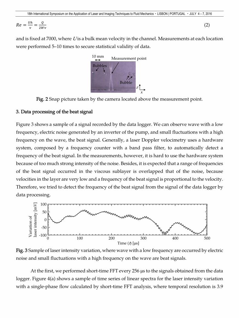
line of bubbles, having 5–12 mm in diameter, passing the measurement point as seen in figure 2.

Reynolds number (Re) in the experiments is defined as

Horizontal channelDiverging converter

Liquid flowmeter PumpWater tank

Injector Measurement point

Two phaseLiquid phase

64h 6h150h

a b

cCamera

Lasersource

Opticalreceiver

zy g

xy g

2h

zx

8h Lasersource

Opticalreceiver

1.5h2θ


𝑅𝑒 =𝑈ℎ

𝜈=

𝑄

2𝑊𝜈 (2)

and is fixed at 7000, where U is a bulk mean velocity in the channel. Measurements at each location

were performed 5–10 times to secure statistical validity of data.

Fig. 2 Snap picture taken by the camera located above the measurement point.

3. Data processing of the beat signal

Figure 3 shows a sample of a signal recorded by the data logger. We can observe wave with a low

frequency, electric noise generated by an inverter of the pump, and small fluctuations with a high

frequency on the wave, the beat signal. Generally, a laser Doppler velocimetry uses a hardware

system, composed by a frequency counter with a band pass filter, to automatically detect a

frequency of the beat signal. In the measurements, however, it is hard to use the hardware system

because of too much strong intensity of the noise. Besides, it is expected that a range of frequencies

of the beat signal occurred in the viscous sublayer is overlapped that of the noise, because

velocities in the layer are very low and a frequency of the beat signal is proportional to the velocity.

Therefore, we tried to detect the frequency of the beat signal from the signal of the data logger by

data processing.

Fig. 3 Sample of laser intensity variation, where wave with a low frequency are occurred by electric

noise and small fluctuations with a high frequency on the wave are beat signals.

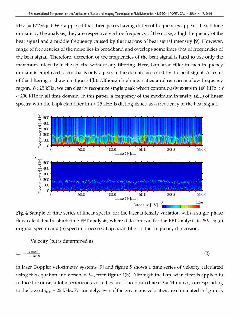
At the first, we performed short-time FFT every 256 μs to the signals obtained from the data

logger. Figure 4(a) shows a sample of time series of linear spectra for the laser intensity variation

with a single-phase flow calculated by short-time FFT analysis, where temporal resolution is 3.9

xz

10 mm

Bubbles

Bubble

Measurement point

0 100 200 300 400 500

100

50

0

-50

-100

Time (t) [μs]

Va

riat

ion

of

lase

rin

ten

sity

[mV

]


kHz (= 1/256 μs). We supposed that three peaks having different frequencies appear at each time

domain by the analysis; they are respectively a low frequency of the noise, a high frequency of the

beat signal and a middle frequency caused by fluctuations of beat signal intensity [9]. However,

range of frequencies of the noise lies in broadband and overlaps sometimes that of frequencies of

the beat signal. Therefore, detection of the frequencies of the beat signal is hard to use only the

maximum intensity in the spectra without any filtering. Here, Laplacian filter in each frequency

domain is employed to emphasis only a peak in the domain occurred by the beat signal. A result

of this filtering is shown in figure 4(b). Although high intensities until remain in a low frequency

region, f < 25 kHz, we can clearly recognize single peak which continuously exists in 100 kHz < f

< 200 kHz in all time domain. In this paper, a frequency of the maximum intensity (fmax) of linear

spectra with the Laplacian filter in f > 25 kHz is distinguished as a frequency of the beat signal.

Fig. 4 Sample of time series of linear spectra for the laser intensity variation with a single-phase

flow calculated by short-time FFT analysis, where data interval for the FFT analysis is 256 μs; (a)

original spectra and (b) spectra processed Laplacian filter in the frequency dimension.

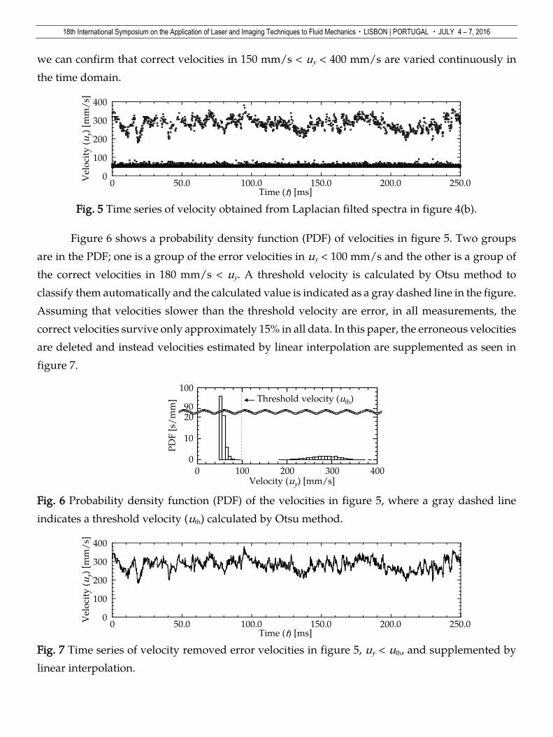
Velocity (uy) is determined as

𝑢𝑦 =𝑓max𝜆

2𝑛 sin𝜃 (3)

in laser Doppler velocimetry systems [9] and figure 5 shows a time series of velocity calculated

using this equation and obtained fmax from figure 4(b). Although the Laplacian filter is applied to

reduce the noise, a lot of erroneous velocities are concentrated near f = 44 mm/s, corresponding

to the lowest fmax = 25 kHz. Fortunately, even if the erroneous velocities are eliminated in figure 5,

0 1.56Intensity [μV]

Time (t) [ms]250.0200.0150.0100.050.00

0

500

300

200

100

400

Fre

qu

ency

(f)

[k

Hz

]

Time (t) [ms]250.0200.0150.0100.050.00

0

500

300

200

100

400

Fre

qu

ency

(f)

[k

Hz]

a

b


we can confirm that correct velocities in 150 mm/s < uy < 400 mm/s are varied continuously in

the time domain.

Fig. 5 Time series of velocity obtained from Laplacian filted spectra in figure 4(b).

Figure 6 shows a probability density function (PDF) of velocities in figure 5. Two groups

are in the PDF; one is a group of the error velocities in uy < 100 mm/s and the other is a group of

the correct velocities in 180 mm/s < uy. A threshold velocity is calculated by Otsu method to

classify them automatically and the calculated value is indicated as a gray dashed line in the figure.

Assuming that velocities slower than the threshold velocity are error, in all measurements, the

correct velocities survive only approximately 15% in all data. In this paper, the erroneous velocities

are deleted and instead velocities estimated by linear interpolation are supplemented as seen in

figure 7.

Fig. 6 Probability density function (PDF) of the velocities in figure 5, where a gray dashed line

indicates a threshold velocity (uth) calculated by Otsu method.

Fig. 7 Time series of velocity removed error velocities in figure 5, uy < uth, and supplemented by

linear interpolation.

Time (t) [ms]250.0200.0150.0100.050.00

0

300

200

100

400

Vel

oci

ty (

uy)

[mm

/s]

Velocity (uy) [mm/s]4003002001000

0

90

10

100

PD

F [

s/m

m]

20

Threshold velocity (uth)

Time (t) [ms]250.0200.0150.0100.050.00

0

300

200

100

400

Vel

oci

ty (

uy)

[mm

/s]


Until here, data processing to obtain time series of velocity from beat signals with low

frequency noises were explained using the beat signal with a single-phase flow. Basically,

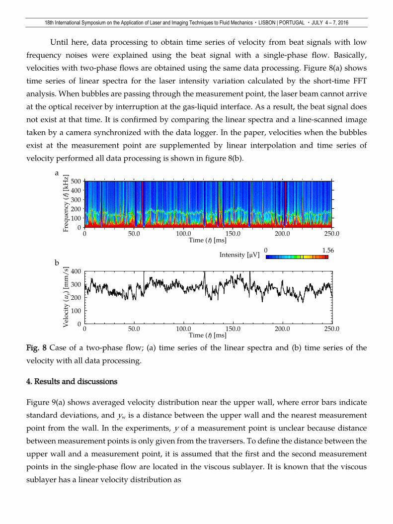
velocities with two-phase flows are obtained using the same data processing. Figure 8(a) shows

time series of linear spectra for the laser intensity variation calculated by the short-time FFT

analysis. When bubbles are passing through the measurement point, the laser beam cannot arrive

at the optical receiver by interruption at the gas-liquid interface. As a result, the beat signal does

not exist at that time. It is confirmed by comparing the linear spectra and a line-scanned image

taken by a camera synchronized with the data logger. In the paper, velocities when the bubbles

exist at the measurement point are supplemented by linear interpolation and time series of

velocity performed all data processing is shown in figure 8(b).

Fig. 8 Case of a two-phase flow; (a) time series of the linear spectra and (b) time series of the

velocity with all data processing.

4. Results and discussions

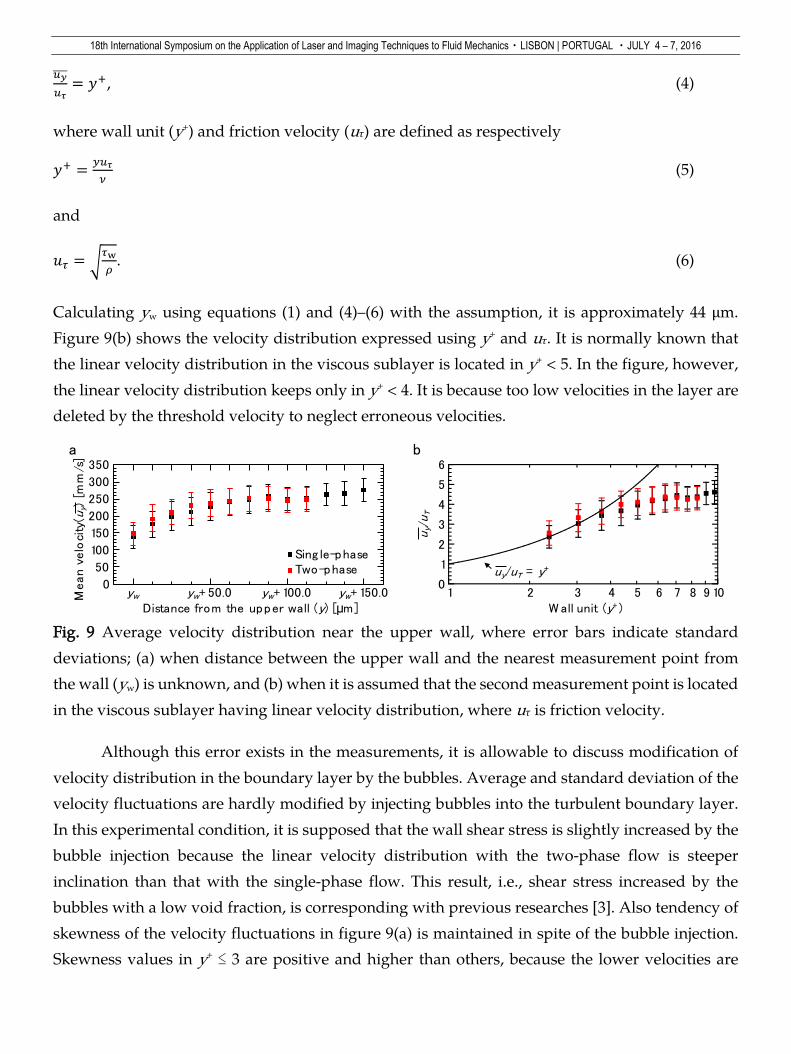
Figure 9(a) shows averaged velocity distribution near the upper wall, where error bars indicate

standard deviations, and yw is a distance between the upper wall and the nearest measurement

point from the wall. In the experiments, y of a measurement point is unclear because distance

between measurement points is only given from the traversers. To define the distance between the

upper wall and a measurement point, it is assumed that the first and the second measurement

points in the single-phase flow are located in the viscous sublayer. It is known that the viscous

sublayer has a linear velocity distribution as

0 1.56Intensity [μV]

b

Time (t) [ms]250.0200.0150.0100.050.00

0

500

300

200

100

400

Fre

qu

ency

(f)

[k

Hz

]a

Time (t) [ms]250.0200.0150.0100.050.00

0

300

200

100

400

Vel

oci

ty (

uy)

[mm

/s]


𝑢𝑦̅̅ ̅̅

𝑢𝜏= 𝑦+, (4)

where wall unit (y+) and friction velocity (uτ) are defined as respectively

𝑦+ =𝑦𝑢𝜏

𝜈 (5)

and

𝑢𝜏 = √𝜏w

𝜌. (6)

Calculating yw using equations (1) and (4)–(6) with the assumption, it is approximately 44 μm.

Figure 9(b) shows the velocity distribution expressed using y+ and uτ. It is normally known that

the linear velocity distribution in the viscous sublayer is located in y+ < 5. In the figure, however,

the linear velocity distribution keeps only in y+ < 4. It is because too low velocities in the layer are

deleted by the threshold velocity to neglect erroneous velocities.

Fig. 9 Average velocity distribution near the upper wall, where error bars indicate standard

deviations; (a) when distance between the upper wall and the nearest measurement point from

the wall (yw) is unknown, and (b) when it is assumed that the second measurement point is located

in the viscous sublayer having linear velocity distribution, where uτ is friction velocity.

Although this error exists in the measurements, it is allowable to discuss modification of

velocity distribution in the boundary layer by the bubbles. Average and standard deviation of the

velocity fluctuations are hardly modified by injecting bubbles into the turbulent boundary layer.

In this experimental condition, it is supposed that the wall shear stress is slightly increased by the

bubble injection because the linear velocity distribution with the two-phase flow is steeper

inclination than that with the single-phase flow. This result, i.e., shear stress increased by the

bubbles with a low void fraction, is corresponding with previous researches [3]. Also tendency of

skewness of the velocity fluctuations in figure 9(a) is maintained in spite of the bubble injection.

Skewness values in y+ ≤ 3 are positive and higher than others, because the lower velocities are

Distance from the upper wall (y) [μm]yw+ 150.0yw+ 100.0yw+ 50.0yw

0

200

100

50

350

Mean v

elo

city

(uy)

[m

m/s

]

150

300

250

a

W all unit (y+ )9531

0

4

2

1

6

uy/

uτ

3

5

b

742 106 8

uy/uτ = y+

Sing le-phaseTwo-phase


deleted together with error velocities when the data processing is performed. Even if we consider

skewness values in y+ > 4, obvious modification of skewness is not observed. However, tendency

of kurtosis in figure 9(b) is dramatically modified by the bubble injection. In the figure, the kurtosis

is defined as kurtosis of Gaussian distribution becomes zero. In the single-phase flow, the kurtosis

decreases when location of the measurement point becomes closer to the upper wall. Contrary to

this, the kurtosis with two-phase flow increases. By these statistical analyses, it is confirmed that

even if bubbles in the turbulent boundary layer are with a low void fraction, characteristics of

velocities in the layer are modified by them.

Fig. 10 Statistical analysis for time series of velocities near the upper wall; (a) skewness and (b)

kurtosis, where the kurtosis is defined as kurtosis of Gaussian distribution becomes zero.

5. Conclusions

We developed a laser Doppler velocimetry system with a high spatio-resolution, 19 μm in the

vertical direction, to access a turbulent boundary layer in a horizontal channel flow and estimated

effects of bubbles injected into the layer on the velocity distribution in the layer. In the

measurements, the system was influenced by electric noise generated by an inverter system of a

pump which is to control a flowrate in the channel. Because beat signals used for calculating

velocities in the system are corrupted by the noise with relatively lower frequencies than that of

the beat signals, a frequency counter with a band pass filter, which is normally used to a laser

Doppler velocimetry, is not useable for detecting automatically a frequency of the beat signals.

Therefore, we also devised a data processing to calculate velocities automatically from the beat

signals with the noise using a short-time FFT analysis and a statistical analysis. Velocity

distributions with a single-phase flow and a two-phase flow were investigated by the laser

Doppler velocimetry system with the data processing, and were estimated using statistical values,

such as average, standard deviation, skewness and kurtosis. In spite of bubble injection, other

statistical values excepting the kurtosis are keeping their values before the bubble injection

W all unit (y+ )

-0.5

0.5

1.5

skew

ness

0

1.0

a

W all unit (y+ )

100-1.0

0

-0.5

0.5

kurt

osi

s

b

42 126 8100 42 126 8

Sing le-phaseTwo-phase


because injected bubbles had too low void fraction. However, the kurtosis with a condition of the

bubble injection shows distinctly different tendency comparing with that with a single-phase flow.

In the single-phase flow, the kurtosis, which defines that Gaussian distribution is zero, has

negative values and decreased when a measurement point becomes close to the wall. In the two-

phase flow, on the contrary, it increases when the measurement point becomes close to the wall,

and has finally positive values. By these analyses, it is confirmed that although bubbles in a

turbulent boundary layer are with a low void fraction, they have a potentiality enough to change

characteristics of velocities in the layer.

Acknowledgment

This work was supported by Grant-in-Aid for JSPS Fellows No. 15J00147 and JSPS KAKENHI

Grant Nos. 24246033 and 23760143. The authors would like to express their appreciation for these

supports.

Reference

[1] Madavan NK, Deutsch S, Merkle CL (1984) Reduction of turbulent skin friction by

microbubbles. Phys Fluids 27:356–363

[2] McCormick ME, Bhattacharyya R (1973) Drag reduction of a submersible hull by electrolysis.

Nav Eng J 85:11–16

[3] Ceccio SL (2010) Frictional drag reduction of external flow with bubble and gas injection. Annu

Rev Fluid Mech 42:183–203

[4] Murai Y (2014) Frictional drag reduction by bubble injection. Exp Fluids 55:1733

[5] van den Berg TH, van Gils DPM, Lathrop DP, Lohse D (2007) Bubbly turbulent drag reduction

is a boundary layer effect. Phys Rev Lett 98:084501

[6] Murai Y, Oishi Y, Takeda Y, Yamamoto F (2006) Turbulent shear stress profiles in a bubbly

channel flow assessed by particle tracking velocimetry. Exp Fluids 41:343–352

[7] Hara K, Suzuki T, Yamamoto F (2011) Image analysis applied to study on frictional drag

reduction by electrolytic microbubbles in a turbulent channel flow. Exp Fluids 50:715–727

[8] Park HJ, Tasaka Y, Murai Y (2015) Ultrasonic pulse echography for bubbles traveling in the

proximity of a wall. Meas Sci Technol 26:125301

[9] Stevenson WH (1992) Laser Doppler velocimetry: A status report. Proc IEEE 70:652–658

Short-time FFT based laser Doppler velocimetry for bubbly...

Documents

Transcript of Short-time FFT based laser Doppler velocimetry for bubbly...