Inﬂuence of surface roughness on the turbulent...

18th International Symposium on the Applications of Laser and Imaging Techniques to Fluid Mechanics · LISBON | PORTUGAL · JULY 4-7, 2016

Influence of surface roughness on the turbulent properties

in the wake of a turbine blade

L. Neuhaus1 , P. Gilge1, J.R. Seume1 and K. Mulleners21 Institute of Turbomachinery and Fluid Dynamics, Leibniz University Hanover, Germany

2 Institute of mechanical engineering, École polytechnique fédérale de Lausanne, Switzerland

Keywords: piv, turbulence, roughness, anisotropy invariant map, Reynolds stress, friction loss

ABSTRACT

The objective of this investigation is to relate the friction loss and turbulence properties in the wake flow of turbine

blades to local surface roughness patches of different chord wise extent. Stereo particle image velocimetry (PIV) is

conducted in the wake of smooth and roughened turbine blades in a cascade windtunnel. Roughness on the blade

surface interacts with the local boundary layer flow. This interaction leads to an increased friction loss due to higher

turbulent kinetic energy. To investigate the connection of friction loss and turbulence, the following methodology is

developed. The friction loss coefficient is directly determined from the PIV data according to Zhang et al. [2003]. The

turbulent kinetic energy is calculated based on the normal Reynolds stresses. The anisotropy invariant map (AIM)

represents the distribution of the turbulence states. In addition to the AIM, which contains no information about

the spatial orientation of the turbulence, a new representation is introduced. This representation allows visualizing

the anisotropic characteristics of the turbulence as well as the preferred spatial direction of anisotropy. The normal

Reynolds stresses are normalized by the turbulent kinetic energy and presented against each other in a triangular

arrangement. Results show an increased friction loss for increased roughness extent. The turbulent kinetic energy on

the suction side of the wake are compared for the roughened and smooth blades. High turbulent kinetic energy is

found in the wake center near the trailing edge of the blade. The turbulent kinetic energy decreases downstream. For

roughened blades, the high turbulent kinetic energy regions extend further downstream than for the smooth blade.

The overall turbulent kinetic energy for the roughened blades is higher than for the smooth blade and increases with

roughness extent.

1. Introduction

Turbomachines are complex mechanical and fluid dynamical systems. The internal flow is turbulent,

inherently unsteady, and three dimensional. Surface roughness on the turbine or compressor blades

can alter the flow properties and overall turbine or compressor efficiency. Surface roughness on

engine blades affects the individual blade by increasing the boundary layer momentum loss

and blade skin friction and by precipitating boundary layer transition [Stieger and Hodson,

2004, Hodson and Howell, 2005]. The blade surface can be roughened due to operational and


environmental conditions or manufacturing and repair processes [Bons et al., 2001]. In both

cases, this results in an inhomogeneous surface roughness characterized by local variations in the

roughness height and orientation [Taylor, 1990, Hohenstein and Seume, 2013]. These multi-scale

roughness topologies can have significant effect on the aerodynamic performance of aero-engine

blades and the turbulent wake flow [Chow et al., 2005]. Accurate estimation of the effect of

multi-scale surface roughness topologies is challenging due to the large number of parameters

involved and the complex interactions between the surface roughness and the boundary layer [Bons,

2010]. In particular, the local boundary layer and surface roughness interactions are influenced by

the height of the local roughness, the thickness and state of the boundary layer, the local pressure

gradient, the extent and distribution of the roughness itself. The Reynolds number also plays an

important role in aircraft engines. If the Reynolds number at fixed stagnation conditions is increased

from 10

5 to 10

7, the maximum height which the surface roughness can have without effecting the

flow is 1.5 times higher [Goodhand, 2015]. However, if this threshold height is exceeded, the losses

increase with increasing Reynolds number. For sand grain roughness applied to a turbine vane,

the losses were found to double for Reynolds numbers increasing from 1.8 · 10

5 to 1.8 · 10

6 [Boyle

and Senyitko, 2003]. Also, the position of transition changed. For a higher Reynolds number, the

laminar to turbulent boundary layer transition on the blade moves upstream. As an result, the

integral boundary layer momentum loss increases, yielding increased friction losses.

For uniform roughness in a rectangular channel, higher Reynolds stresses, turbulent kinetic energy,

and momentum transport in the boundary layer flow can be detected [Barros and Christensen, 2014,

Vanderwel and Ganapathisubramani, 2015, Mejia-Alvarez and Christensen, 2013]. Higher Reynolds

stresses result from higher fluctuations in the wall normal velocity. The fluctuations are initiated by

the surface roughness and spread into the outer region of the boundary layer [Bhaganagar et al.,

2004]. The state of the turbulence can change due to surface roughness. In the near-wall region of a

smooth wall, anisotropic Reynolds stresses are present which become more isotropic when surface

roughness increases [Antonia and Krogstad, 2001].

To understand the interactions of surface roughness and the boundary layer flow, it is desirable to

investigate the influence of local changes in the surface roughness and their effect on the overall

loss behavior of airfoils. Previous investigations by the authors have focused on the influence of

the location of surface roughness patches and their combined effect on the aerodynamic losses

[Mulleners et al., 2014]. Local surface roughness was applied at different positions on the suction

side of turbine blades. For every location, an increase in friction loss and the accompanied variation


in the wake parameters was observed. The wake size increased and the deflection angle changed

depending on the location of the roughness. The results show that each local roughness position has

an individual effect on the resulting wake flow and the overall aerodynamic loss [Mulleners et al.,

2014]. For combinations of localized surface roughness patches, an increase of the losses was found,

which did not equal the mere sum of the losses observed for the individual roughness patches. A

combined effective chord normal distance was introduced as a scaling parameter to estimate the

combined loss effect. The strongest influence on the friction loss was found for roughnesses near

the region where the chord-wise pressure gradient changes sign [Gilge and Mulleners, 2016]. This

is in good agreement with results of Shin and Jin Song [2014a,b], who showed that a favorable

pressure gradient damps the effect of surface roughness on the losses whereas an adverse pressure

gradient amplifies it. The destabilization leads to faster boundary layer growth and spreading of

disturbances.

Following up on the previous work, this paper focuses on the influence of the chord-wise extent

of localized roughness patches on aerodynamic properties of the turbine blade wake flow and

the friction coefficient. Special attention is given to the turbulence properties in the wake of the

turbine blade. The objective of this study is to develop a flow diagnostic strategy which allows

for the determination of the skin friction coefficient and its fluid dynamical cause directly from

velocity field data in the turbine blade wake. The distribution of turbulence properties is analyzed

by means of the anisotropy invariant map. Additionally, the different Reynolds stress components

are compared to obtain information about the turbulence state and the anisotropic direction. Oil

flow visualizations are combined with PIV data in order to directly relate local boundary layer

effects with variations in the turbulent properties of the wake flow and global changes in the friction

loss.

2. Experimental set-up

2.1 Hardware

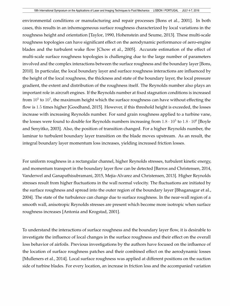
Experiments are conducted in the linear cascade wind tunnel of the Institute of Turbomachinery

and Fluid Dynamics of the Leibniz Universität Hannover (figure 1). The flow medium is air. The air

has a constant temperature of 298 K ± 5 K and is guided through flow straighteners and a settling

chamber to generate a homogeneous inflow with a turbulence intensity of 4.5 % in the cascade inlet

plane.

The middle blade is split into two parts, where one part is a reference blade and the mirrored

blade is the test blade. The reference blade remains the same for all investigations. The test blade


Figure 1: Linear cascade wind tunnel.

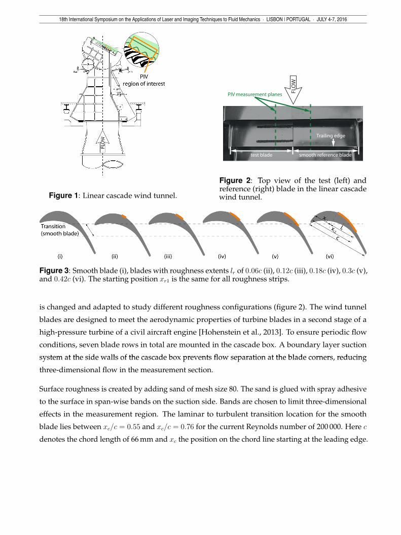
Figure 2: Top view of the test (left) andreference (right) blade in the linear cascadewind tunnel.

Figure 3: Smooth blade (i), blades with roughness extents lr

of 0.06c (ii), 0.12c (iii), 0.18c (iv), 0.3c (v),and 0.42c (vi). The starting position x

r1 is the same for all roughness strips.

is changed and adapted to study different roughness configurations (figure 2). The wind tunnel

blades are designed to meet the aerodynamic properties of turbine blades in a second stage of a

high-pressure turbine of a civil aircraft engine [Hohenstein et al., 2013]. To ensure periodic flow

conditions, seven blade rows in total are mounted in the cascade box. A boundary layer suction

system at the side walls of the cascade box prevents flow separation at the blade corners, reducing

three-dimensional flow in the measurement section.

Surface roughness is created by adding sand of mesh size 80. The sand is glued with spray adhesive

to the surface in span-wise bands on the suction side. Bands are chosen to limit three-dimensional

effects in the measurement region. The laminar to turbulent transition location for the smooth

blade lies between x

c

/c = 0.55 and x

c

/c = 0.76 for the current Reynolds number of 200 000. Here c

denotes the chord length of 66 mm and x

c

the position on the chord line starting at the leading edge.

















c

/c = 0.55 and x

c



c




FLO

W

test blade smooth reference blade

PIV measurement planes

Trailing edge















c

/c = 0.55 and x

c



c



2.2 Measurement cases

In this study, six cases are compared including a smooth and five cases with the chord-wise

roughness band extents lr

= 0.06c (ii), lr

= 0.12c (iii), lr

= 0.18c (iv), lr

= 0.3c (v), and l

r

= 0.42c (vi)

(figure 3). The starting location x

r1 of the roughness bands is located 0.06c upstream of the location

where the chord-wise pressure gradient changes sign. The roughnesses are varied in chord-wise

extent lr

= x

r1 � x

r2, i.e. the distance between the chord-wise starting location x

r1 and ending

location x

r2 of the roughness bands (figure 3). The roughness extent is increased downstream into

the region with an adverse pressure gradient. These cases are chosen because roughness near the

location where the pressure gradient changes sign tends to have the strongest influence on the

friction loss [Gilge and Mulleners, 2016]. The loss is expected to increase with increasing roughness

extent lr

.

2.3 Measurement techniques

Stereo particle image velocimetry (PIV) is conducted to determine the velocity field in the wake

of the roughened test blade and the smooth reference blade. Two sCMOS cameras equipped with

Scheimpflug adapters are used. The oil particles in the flow are illuminated by a double-pulsed laser

with a pulse rate of 15 Hz and a maximum energy of 200 mJ/pulse. To measure on the roughened

test blade side and the smooth reference blade side successively without having to recalibrate or

switch the wind tunnel off and on, the entire PIV system, i.e. the light sheet and the cameras, is

traversed accurately between the two measurement locations. To do so, the PIV setup is mounted

on an aluminum rail system and connected to a linear drive. The results become unaffected by

potential variations in operating conditions resulting from switching the wind tunnel off and on,

as the results from the roughened blade side and the smooth reference blade side can be directly

compared. For every case 1000 PIV double images are recorded. The double images are evaluated

by a multi grid algorithm with a final interrogation window size of 24px x 24px and an overlap of

62.5% resulting in a physical resolution of 0.5 mm, i.e. 0.0076c.

In addition to PIV, oil flow visualization is conducted. The oil flow visualizations indicate the

presence and location of the separation bubble and the location of the laminar to turbulent transition.

To determine the pressure gradient on the suction side of the blade, pressure measurements of the

smooth blade are conducted by eleven surface pressure probes at the suction side.

3. Results

As an integral part of this paper, a data analysis strategy is developed to identify and characterize

the influence of the roughness strips’ extent on the friction losses, the wake geometry and turbulence

properties, and the connection between them, based on stereo PIV.


wake

centerline

x

g

�

c

wake

region of interest

x

1

y

g

x2λ

1.05

1

0.95

0.9

0.85

0.8

UU∞

Figure 4: Velocity field in the wake region of interest including the wake centerline and wakecoordinate system.

3.1 Wake region of interest

To calculated the wake parameters, the velocity field determined by PIV is transformed from the

global cascade wind tunnel coordinate system (xg

, y

g

) into the wake orientated coordinate system

(x1, x2) similar to the approach described by Gilge and Mulleners [2015] (figure 4). In the wake

coordinate system, the axis x1 is defined by the centerline of the wake with x2 perpendicular to it.

The axis x1 is pointing in mean flow direction. The centerline is determined by a least square fit of

the minimum velocity locations in the wake. The PIV data is presented and further analyzed in the

wake region of interest (figure 5). The analysis includes the determination of wake width, the friction

loss and, turbulent properties, i.e. kinetic energy, anisotropy, and the dominant spatial direction of

the turbulence. The velocity on the suction side of the wake is compared for the roughened blades

and their respective smooth reference blades (figure 5). The upper part shows the velocity for the

roughened test blade and the lower part the mirrored velocity for the smooth reference blade. An

increased roughness extent lr

leads to an increased velocity deficit in the wake compared to the

reference blade. For all roughness extents, the dimensionless velocity magnitude U

U1with U1, the

freestream velocity, in the wake is lower than the velocity magnitude in the wake of the smooth

reference blade. With increasing roughness extent the wake width � is also increasing. The cross

section which is located 0.6c downstream the turbine blade is extracted to further determine the

wake width � and the friction loss.

3.2 Loss coefficient

To compare the friction loss for the different cases, the friction loss coefficient �⇣ is determined

directly from the wake velocity field based on the control volume approach described by Zhang

et al. [2003] as previously applied by Gilge and Mulleners [2016]. The described method allows to

directly extract integral values, i.e. the friction loss coefficients �⇣ , from the PIV data.


0.8 0.85 0.9 0.95 1 1.05

U

U1

�0.1

0

0.1

x

2c

�0.1

0

0.1

x

2c

�0.1

0

0.1

x

2c

�0.1

0

0.1

x

2c

0.2 0.4 0.6 0.8 1

�0.1

0

0.1

x1c

x

2c

test blade

reference blade

Figure 5: Dimensionless wake velocity U

U1on the suction side of the wake of the test blade for

different roughness extents and the respective reference blade.

An increasing roughness extent lr

is leading to an increasing loss coefficient �⇣ (figure 6). However,

the loss coefficient �⇣ for the highest roughness extent lr

= 0.42c is lower than the loss coefficient

for the second highest roughness extent lr

= 0.3c. The magnitudes of the loss coefficient �⇣ are in

good agreement with previous results of locally applied roughness patches on a turbine profile

[Gilge and Mulleners, 2016]. In the following, properties will be presented as a function of the loss

coefficient �⇣ .


0 0.1 0.2 0.3 0.4

0

0.01

0.02

0.03

0.04

lrc

�⇣

smoothl

r

= 0.06c

l

r

= 0.12c

l

r

= 0.18c

l

r

= 0.30c

l

r

= 0.42c

Figure 6: Loss coefficient �⇣ in function of the roughness extent lrc

.

3.3 Wake width

The wake width � is determined by the distance between the locations on suction and pressure

side of the wake where 95% of the freestream velocity U1 is reached. The distance is calculated

perpendicular to the wake centerline for every stream-wise position x1 in the wake region of interest.

The change of wake width is approximated by a linear fit. To compare the different cases, the

wake width is determined at the position 0.6c downstream of the turbine blade. To reduce the

influence of switching the wind tunnel on and off, the wake width of the roughened test blade �

test

is normalized by the wake width of the reference blade �

ref

and compared to the smooth case. This

normalized wake width

�w =

�test�ref

��rough

�test�ref

��smooth

(1)

allows for the direct comparison of the wake width of the different cases (figure 7).

The wake width increases almost linearly with increasing loss coefficient, except of the second

smallest roughness extent lr

= 0.12c, where the wake width is smaller than expected. For the largest

extent, the wake width has recovered with respect to the third largest extent, which corresponds to

a decrease of the loss coefficient.

The increased friction loss is caused by a change in the blade’s suction side boundary layer. This


0 0.01 0.02 0.03 0.04

0.9

1

1.1

1.2

1.3

1.4

1.5

�⇣

�w

smoothl

r

= 0.06c

l

r

= 0.12c

l

r

= 0.18c

l

r

= 0.30c

l

r

= 0.42c

Figure 7: Normalized wake width �w 0.6c downstream of the turbine blade in function of the losscoefficient �⇣ .

can be observed by the oil flow visualization (figure 8). The leading edge is located on the left of the

image and flow is going from left to right. For the smooth blade, the first half of the blade shows a

smooth distribution of the oil (a)(figure 8 (i)). In this region the boundary layer is laminar and the

pressure gradient dcpdxc

is negative, i.e. favorable, up to the point (b) (figure 8 (iv)). The gradient of

the pressure coefficient is calculated based on the pressure measurements on the smooth blade. The

pressure gradient dcp

dxcon the suction side is negative up to x

c

/c = 0.35. Thereafter, the stream-wise

pressure gradient changes sign and stays positive. In the region of highest flow velocity, there is a

band with low pigment density (b). Due to a higher shear rate caused by higher acceleration, the oil

has mostly vanished. Behind the laminar region, the flow separates because it cannot overcome

the adverse pressure gradient (figure 8 (iv)). The start of the separation bubble is indicated by a

span-wise line of accumulated oil (c). The separated shear layer is unstable and laminar turbulent

transition begins slightly downstream of the separation. As this change of the boundary layer

state allows a higher transport of momentum into the boundary layer, this leads to reattachment

of the turbulent boundary layer. The end of the separation bubble is characterized by a flake-like

distribution of the oil (d). Here, the reattaching flow forces the pigments to spread out. Further

downstream, the boundary layer is completely reattached (e).

For the roughened blades, the visualization is limited by the roughness, as the oil sticks to the


Figure 8: Oil flow visualization of the smooth blade (i), and blades with the roughness extents ofl

r

= 0.06c (ii) and l

r

= 0.42c (iii). The pressure gradient dcpdxc

is determined by pressure measurementson the suction side of the smooth blade (iv).

sand grains and no oil structure can be recognized on the roughness location (figure 8 (ii,iii)). The

oil flow visualization indicates no separation bubble for the roughened blades. The roughnesses

upstream of the location for the separation bubble of the smooth blade now seem to trigger the

laminar turbulent transition at the start of the roughness patch. As the turbulent boundary layer

exhibits a higher momentum transport, the kinetic energy in it is higher and it can overcome the

adverse pressure gradient without separating.

For the roughened blade, the turbulent boundary layer flow covers a larger portion of the blade

surface than for the smooth blade. This leads to an increase in friction, as turbulent boundary layer

flow experiences a higher surface friction than its laminar counterpart.


3.4 Turbulence analysis

Knowledge of the turbulence stresses, their anisotropy, and the magnitude of the turbulent kinetic

will help to identify sources of increased losses.

To quantify turbulence in the wake of the turbine blade, the components of the Reynolds stress

tensors

R

ij

= u

0i

u

0j

(2)

are calculated. Here u

0i

and u

0j

are the fluctuating parts of the i-th and j-th velocity components

and indicates the ensemble average over all available snapshots. The Reynolds stress tensor

provides information on the different components of turbulence and provides a measure for the

turbulent momentum transport. It allows to determine the relative strength of different fluctuation

components. When i = j, the normal turbulent stress is considered and when i 6= j a tangential

turbulent stress is meant. The turbulent kinetic energy is defined as

k =

1

2

q

2=

u

0i

u

0i

2

, (3)

with q

2, the trace of the Reynolds stress tensor.

The turbulent kinetic energy on the suction side of the wake is compared for the roughened blades

and their respective smooth reference blades (figure 9). The upper part shows the turbulent kinetic

energy for the roughened test blade and the lower part the mirrored turbulent kinetic energy for the

smooth reference blade. The highest turbulent kinetic energy is found close to the trailing edge of

the blade. In general, the turbulent kinetic energy is higher in the center of the wake and decreases

downstream. Normal to the mean flow direction, the turbulent kinetic energy decreased faster than

in flow direction. The turbulent kinetic energy behind the roughened blades is higher in the core

than the turbulent kinetic energy behind the reference blade. With increasing roughness extent

this ratio increases. For higher roughness extent, a higher turbulent kinetic energy concentration is

found in a larger downstream area than for the smooth reference blade.

The turbulent kinetic energy holds no information about the turbulence state, i.e. the distribution

of the turbulent kinetic energy on the Reynolds stress components. The Reynolds stress tensor

includes this information. To directly compare the different components the anisotropy invariant

map is used. The anisotropy invariant map (AIM) was first introduced by Lumley and Newman

[1977] and allows for a characterization of the state of turbulence by the amount of anisotropy.

Anisotropy refers to different magnitudes of the fluctuation components. The components of the


k [m2/s2] > 5 > 10 > 15 > 20

�0.1

0

0.1

x

2c

�0.1

0

0.1

x

2c

�0.1

0

0.1

x

2c

�0.1

0

0.1

x

2c

0.2 0.4 0.6 0.8 1

�0.1

0

0.1

x1c

x

2c

test blade

reference blade

Figure 9: Turbulent kinetic energy on the suction side of the wake of the test blade for differentroughness extents and the respective reference blade.

anisotropy tensor are given by

b

ij

=

u

0i

u

0j

q

2� 1

3

�

ij

(4)

where �

ij

is the Kronecker delta. With the anisotropy tensor the anisotropy invariants

II = b

ij

b

ji

(5)

III = b

ij

b

in

b

jn

(6)


II

III0 2/9-1/36

2/3

1/6

axisymmetricII = 3/2 (4/3 III)2/3

1D

isotropicaxisymmetricII = -3/2 (4/3 III)2/3

2DII=2/9+2III

axisymmetric 2D

Figure 10: The anisotropy invariant map for defines every state of turbulence by its dimensionality(adapted from [Lumley and Newman, 1977]).

can be calculated using the Einstein summation convention. The anisotropy invariant map thus

visualizes the non-uniformity of the momentum transport by the fluctuations in the different

spatial directions (figure 10). All realizable anisotropy invariant combinations must lie in the area

defined in this map between the three boundaries, which mark the limiting physical bounding

states of turbulence. The limiting states are defined by two-dimensional II =

29 + 2III and

axisymmetric turbulence II =

32(

43 |III|)

23 . For the axisymmetric state, the magnitudes of the

turbulence components in two dimensions are equal, whereas the magnitude of the third component

differs. One boundary is found for the cases where the third component is larger than the other

components, i.e. "cigar" shaped turbulence. The other axisymmetric boundary is found for the

cases where the third component is smaller than the other components, i.e. disk shaped turbulence.

The third boundary is defined by the two-dimensional state. Turbulence in this state has only

two components. The corners are defined by the extrema of the boundaries, being isotropic,

axisymmetric two-dimensional, and one-dimensional turbulence. The isotropic state is defined by a

equally distributed magnitude of turbulence components in all dimensions. If the magnitudes of

the turbulence components differ, anisotropic states occur.

In general, the AIM for the different roughness extents indicate a predominantly isotropic turbulence

(figure 11). The difference between the test blades and the reference blades is small. For all roughness

extents, isotropic turbulence and slightly axisymmetric turbulence, cigar shaped as well as disk

shaped, are present.


0

0.05

0.1

0.15

II

0

0.05

0.1

0.15

II

�0.01 �0.005 0 0.005 0.01 0.015

III

�0.01 �0.005 0 0.005 0.01 0.015

0

0.05

0.1

0.15

III

II

test bladereference blade

Figure 11: Anisotropy invariant map for different roughness extents.

The AIM gives information about the anisotropy and the dimensionality of the turbulence, but not

about which turbulence component is dominant.

To extract information about the orientation of the turbulence state and visualize its changes due to

various surface roughness distributions, a new representation is introduced (figure 12).

In this representation, the components of the normal turbulent stresses u

01u

01, u0

2u02, and u

03u

03 are

normalized by twice the turbulent kinetic energy 2k = u

0i

u

0i

and presented in the turbulence triangle

(figure 12). For each component, an axis is defined reaching from the opposing triangle leg to the

triangle corner and ranging from 0 to 1. A state can be determined by just two axes and the third

component can be directly determined from the two others as a result of the normalization by 2k.

Isotropic turbulence is now found at the intersection of the three axes where all normal turbulent

stresses are of the same size. Each axis defines an axisymmetric turbulence state.

In the upper part of the triangle points on the green axis exhibit a high portion of turbulence in x1

direction. Fluctuations in x2 and x3 direction have the same magnitude. Hence, the turbulence state


Figure 12: Normalized normal Reynolds stresses defining different turbulence states andadditionally the direction of the turbulence dimensionality.

is cigar shaped in x1 direction. In the lower part of the triangle, the portion of turbulence in x1 is low.

The turbulence here is disk shaped. This is valid for each axis. The boundaries of the triangle give

the states where at least one component is zero and define two-dimensional turbulence states. The

extrema are reached at the corners of the triangle where two components are zero and turbulence

is one-dimensional. This representation allows to convey information about the direction of the

turbulence in addition to the turbulence state.

The roughened blades show similar turbulence states in the turbulence triangle as determined by

the AIM (figure 13). The turbulence is mainly isotropic. Additionally, further information about the






















reference bladetest blade

Figure 13: Normalized Reynolds stresses for different roughness extents.

direction of the turbulence can be obtained. The fluctuations in mean flow direction differ the most.

The fluctuations in vertical direction are higher than fluctuations in lateral direction.


u

02u

02

2k

u

03u

03

2k

u

01u

01

2k

�

M

Figure 14: Mean values of the normalized Reynolds stresses

To define the change of the turbulent state between the smooth and the roughened blade, the mean

values of the normalized turbulent normal stress distribution are determined (figure 14). To get

a value for the anisotropy of the turbulence, the anisotropy rate M is determined by the distance

between the isotropic and the mean turbulence state (figure 14). For the dominant turbulence

direction � of the turbulence state, the angle between the axis in mean flow direction u

01u

01

2k and the

line between isotropic and the mean turbulence location is determined. Depending on the angle, the

mean turbulence is of different state and direction. For an angle of 0

�, the turbulence is cigar shaped

in mean flow direction and the state and direction changes continuously for every 60

� (figure 12).

For the test blades, the turbulence tends to be slightly more cigar shaped in x2 direction as the

predominant turbulence indicates u02u

02 as the highest fluctuation. The anisotropy rate M is low for

all cases, as determined by the AIM. It tends to decrease with increasing loss coefficient (figure 15).

The predominant turbulence state � slightly differs but in general stays cigar shaped in x2 direction.

The turbulence becomes even more isotropic for a roughened blade.


0 0.01 0.02 0.03 0.04

�0.025

�0.02

�0.015

�0.01

�0.005

0

�⇣

�M

smoothl

r

= 0.06c

l

r

= 0.12c

l

r

= 0.18c

l

r

= 0.30c

l

r

= 0.42c

�15

�10

�5

0

5

10

�[

� ]

Figure 15: The change of the anisotropy rate �M and the turbulence state �� for differentroughness extents in dependence of the loss coefficient �⇣ .

4. Conclusions

In this paper the overall loss behavior of a turbine blade with different roughness cases is studied.

To determine the boundary layer state, oil flow visualization is conducted. The results for the

loss behavior are combined with a turbulence analysis. A method is developed to investigate the

turbulence based on the velocity measurements in the wake region of a turbine blade. To characterize

the state of the turbulence, the anisotropy invariant map by [Lumley and Newman, 1977] is used.

To quantify the anisotropy direction of the turbulence, a new presentation of normalized normal

Reynolds stresses is introduced. This allows defining turbulence by two parameters, i.e. anisotropy

rate and turbulence state.

The portion of the blade where the boundary layer is turbulent is increased by adding roughness,

as the laminar to turbulent transition on the blade is triggered by the roughness. An increased

roughness extent generally leads to an increased friction loss coefficient, as was expected by previous

works. With increasing loss, the low anisotropic turbulence becomes even more isotropic, whereas

the turbulent kinetic energy increases.

The results of this study show that changes in the turbulent flow can be clearly detected in the wake

flow of a turbine blade by PIV. The state of the turbulence structures as well as its spatial direction for

different roughness extents can be determined and becomes more isotropic for increased roughness.


k [m2/s2] > 5 > 10 > 15 > 20

0

0.04

0.08

x

2c

0

0.04

0.08

x

2c

0

0.04

0.08

x

2c

0.2 0.3 0.4 0.5 0.6 0.7 0.8 0.9 1 1.1 1.2 1.3 1.4

0

0.04

0.08

x1c

x

2c

1000 snapshots

2000 snapshots

4000 snapshots

9000 snapshots

Figure 16: Turbulent kinetic energy k of the smooth reference blade in dependence of the numberof snapshots.

5. Outlook

The methodology presented here will be applied in future for different roughness locations and

extents, in addition to the herein mention cases. The objective will be to characterize the loss

coefficient in function of location and roughness extent. Furthermore, the methodology will be

applied to compressor blades where surface roughness has a larger effect. The goal will be to

provide further insight into the physical mechanisms leading to increased friction loss by roughness.

Further investigations will focus on connecting the surface roughness effect on the turbulence

properties in the wake with the direct effects in the surface boundary layer. To study the complete

causal chain of turbulence production by surface roughness and the subsequent convection into

the wake, near surface measurements by means of PIV combined with numeric simulations will be

undertaken. To visualize the influence of the number of snapshots on the determined turbulent

kinetic energy distribution in the wake, the snapshots for the reference blade are averaged over 1,

2, 4 and 9 measurement sets (figure 16). Further investigations will be undertaken with an even

higher number of snapshots, as the distribution of the turbulent kinetic energy becomes smoother

for an higher amount of snapshots.

Acknowledgements

This work has been conducted within the framework of subproject B3 entitled Influence of complex

surface structures on the aerodynamic loss behaviour of blades of the Collaborative Research Centre

(CRC) 871 Regeneration of Complex Capital Goods funded by the German Research Foundation (DFG).


References

R.A Antonia and P-Å Krogstad. Turbulence structure in boundary layers over different types of

surface roughness. Fluid Dynamics Research, 28(2):139 – 157, 2001.

Julio M. Barros and Kenneth T. Christensen. Observations of turbulent secondary flows in a

rough-wall boundary layer. Journal of Fluid Mechanics, 748, 2014.

Kiran Bhaganagar, John Kim, and Gary Coleman. Effect of roughness on wall-bounded turbulence.

Flow, turbulence and combustion, 72(2-4):463–492, 2004.

J. P. Bons. A Review of Surface Roughness Effects in Gas Turbines. Journal of Turbomachinery, 132(2):

021004, 2010.

J. P. Bons, R. P. Taylor, S. T. McClain, and R. B. Rivir. The Many Faces of Turbine Surface Roughness.

Journal of Turbomachinery, 123(4):739, 2001.

R J Boyle and R G Senyitko. Measurements and Predictions of Surface Roughness Effects on the

Turbine Vane Aerodynamics. Proceedings of ASME Turbo Expo, (GT2003-38580), 2003.

Y. C. Chow, O. Uzol, J. Katz, and C. Meneveau. Decomposition of the spatially filtered and ensemble

averaged kinetic energy, the associated fluxes and scaling trends in a rotor wake. Physics of Fluids,

17(8):085102, 2005.

Philipp Gilge and Karen Mulleners. On the resulting aerodynamic loss of combinations of localized

surface roughness patches on a turbine blade. In 33rd AIAA Applied Aerodynamics Conference, 2015.

Philipp Gilge and Karen Mulleners. Resulting aerodynamic losses of combinations of localized

roughness patches on a turbine blade. AIAA Journal- in press, 2016.

Martin N Goodhand. Admissible Roughness in Gas Turbines. Percceedings of ASME Turbo Expo

2015, pages 1–8, 2015.

H. P. Hodson and R. J. Howell. Bladerow Interactions, Transition, and High-Lift Aerofoils in

Low-Pressure Turbines. Annual Review of Fluid Mechanics, 37(1):71–98, 2005.

Sebastian Hohenstein and Joerg R. Seume. Numerical investigation on the influence of anisotropic

surface structures on the skin friction. Number 1933, pages 1–12, 2013.

Sebastian Hohenstein, Jens Aschenbruck, and Jörg Seume. Aerodynamic effects of non-uniform

surface roughness on a turbine blade. Proceedings of ASME Turbo Expo, (GT2013-95433), 2013.


J.L Lumley and G.R. Newman. The return to isotropy of homogeneous turbulence. J. Fluid Mech.,

82(1):161–178, 1977.

R. Mejia-Alvarez and K. T. Christensen. Wall-parallel stereo particle-image velocimetry

measurements in the roughness sublayer of turbulent flow overlying highly irregular roughness.

Physics of Fluids, 25(11):115109, 2013.

K. Mulleners, P. Gilge, and S. Hohenstein. Impact of surface roughness on the turbulent wake flow

of a turbine blade. Journal of Aerodynamics, article ID, 2014.

Ju Hyun Shin and Seung Jin Song. Pressure gradient effects on smooth and rough surface turbulent

boundary layers—part I: Favorable pressure gradient. Journal of Fluids Engineering, 137(1):011203,

2014a.

Ju Hyun Shin and Seung Jin Song. Pressure gradient effects on smooth- and rough-surface turbulent

boundary layers—part II: Adverse pressure gradient. Journal of Fluids Engineering, 137(1):011204,

2014b.

R. D. Stieger and H. P. Hodson. The Transition Mechanism of Highly Loaded Low-Pressure Turbine

Blades. Journal of Turbomachinery, 126(4):536, 2004.

Robert P Taylor. Surface Roughness Measurements on Gas Turbine Blades. ASME Journal of

Turbomachinery, (112):175–180, 1990.

Christina Vanderwel and Bharathram Ganapathisubramani. Effects of spanwise spacing on

large-scale secondary flows in rough-wall turbulent boundary layers. Journal of Fluid Mechanics,

774:R2, 2015.

Q. Zhang, P. M. Ligrani, and S. W. Lee. Determination of rough-surface skin friction coefficients

from wake profile measurements. Experiments in Fluids, 35(6):627–635, 2003.

Inﬂuence of surface roughness on the turbulent...

Documents

Transcript of Inﬂuence of surface roughness on the turbulent...