SHORT-TERM RECURRENCE KRYLOV SUBSPACE METHODS

SIAM J. MATRIX ANAL. APPL. c© 2012 Society for Industrial and Applied MathematicsVol. 33, No. 2, pp. 480–500

SHORT-TERM RECURRENCE KRYLOV SUBSPACE METHODSFOR NEARLY HERMITIAN MATRICES∗

MARK EMBREE† , JOSEF A. SIFUENTES‡ , KIRK M. SOODHALTER§ ,DANIEL B. SZYLD§ , AND FEI XUE§

Abstract. The progressive GMRES algorithm, introduced by Beckermann and Reichel in 2008,is a residual-minimizing short-recurrence Krylov subspace method for solving a linear system in whichthe coefficient matrix has a low-rank skew-Hermitian part. We analyze this algorithm, observing acritical instability that makes the method unsuitable for some problems. To work around this issuewe introduce a different short-term recurrence method based on Krylov subspaces for such matrices,which can be used as either a solver or a preconditioner. Numerical experiments compare this methodto alternative algorithms.

Key words. GMRES, MINRES, nearly Hermitian matrices, low-rank modifications

AMS subject classifications. 65F10, 65N12, 15B57, 45B05, 45A05

DOI. 10.1137/110851006

1. Introduction. A variety of applications warrant the solution of linear sys-tems of equations where the coefficient matrixA has a skew-Hermitian part 1

2 (A−A∗)with low rank. Such systems arise, for example, from discretized integral equationsderived from wave scattering applications and electrostatics [28], as well as path fol-lowing methods [1]. In this paper, we consider efficient Krylov subspace methods forthe solution of

(1.1) Ax = b,

where the nonsingular coefficient matrix A ∈ Cn×n has the structure

(1.2) A = A∗ + FG∗ = H+ 12FG

∗,

for full rank F, G ∈ Cn×s with s� n; H := 12 (A+A∗) is the Hermitian part of A.

Beckermann and Reichel [1] proposed a “progressive GMRES” algorithm basedon a short recurrence for problems with the structure (1.2), which is mathematicallyequivalent to the much less efficient full GMRES method [23]. We have found thatprogressive GMRES, while theoretically elegant, can suffer from fundamental numer-ical instabilities that render it unsuitable for some otherwise benign matrices of theform (1.2). In this paper we carefully document these instabilities and propose an al-ternative algorithm that uses a Schur complement approach to solve systems with this

∗Received by the editors October 11, 2011; accepted for publication April 17, 2012; publishedelectronically June 5, 2012.

http://www.siam.org/journals/simax/33-2/85100.html†Department of Computational and Applied Mathematics, Rice University, Houston, TX 77005–

1892 ([email protected]). This author’s research was supported by the U. S. National Science Foun-dation under grant DMS-CAREER-0449973.

‡Courant Institute of Mathematical Sciences, New York University, New York, NY 10012-1185([email protected]). This author’s research was supported by the U. S. National Science Foun-dation under a Graduate Research Fellowship and grants DMS-CAREER-0449973, DMS06-02235and Air Force NSSEFF Program award FA9550-10-1-018.

§Department of Mathematics, Temple University, Philadelphia, PA 19122-6094([email protected], [email protected], [email protected]). The research of these authorswas supported in part by the U.S. Department of Energy under grant DE-FG02-05ER25672 and theU. S. National Science Foundation under grant DMS-1115520.

480

KRYLOV METHODS FOR NEARLY HERMITIAN MATRICES 481

structure using short-term recurrence relations. While our method is not equivalentto full GMRES for the original system, it is based on an optimal method (MINRES)for the Hermitian part of A, and can be applied as either a solver or a preconditioner.

We begin by introducing progressive GMRES (PGMRES) in the next section.In section 3 we present numerical experiments that demonstrate the instability ofPGMRES for some well-conditioned linear systems, then comment on possible causesfor this instability. We propose in section 4 an alternative algorithm for (1.1)–(1.2)based on existing Schur complement methods. In section 4.1, we use this methodto precondition coefficient matrices that are small-norm perturbations of a matrix ofthe form (1.2). We present numerical experiments in section 5 that compare our newmethod to existing ones.

2. Preliminaries. The GMRES algorithm approximates the solution to (1.1)through an iterative process that, beginning with an initial iterate x0 = 0, constructsat iteration k the vector xk that solves the least squares problem

(2.1) minx∈Kk(A,b)

‖b−Ax‖

over the Krylov subspace Kk(A,b) = span{b, Ab, A2b, . . . ,Ak−1b} [23]. To solvethis problem, an orthonormal basis for the Krylov subspace is developed throughthe Arnoldi process. The first k steps of this procedure can be collected into therelationship

AVk = Vk+1Hk(2.2)

= VkHk + hk+1,kvk+1eTk ,(2.3)

where Vk ∈ Cn×k and Vk+1 := [Vk vk+1] ∈ Cn×(k+1) have orthonormal columns and

Hk ∈ C(k+1)×k is upper Hessenberg with upper k × k block Hk and (k + 1, k) entryhk+1,k. If the Arnoldi process starts with v1 = b/‖b‖, then Kk(A,b) = Ran(Vk),the range of Vk. It is straightforward to then show that (2.1) is equivalent to theleast squares problem

(2.4) minc∈Ck

‖ ‖b‖e1 − Hkc‖,

and xk = Vkck solves (2.1) if ck solves (2.4). Postmultiplying both sides of (2.3) byek, we can write the Arnoldi vector update as

(2.5) hk+1,kvk+1 = Avk −VkHkek,

where hk+1,k = ‖Avk − VkHkek‖ ≥ 0. Computing the updated Arnoldi vectorvk+1 through (2.5) is often carried out via modified Gram–Schmidt orthogonalization(see [22, Chap. 6] for details and alternatives).

Suppose the coefficient matrix is Hermitian, A = A∗. Then the Hessenbergmatrix is also Hermitian, Hk = V∗

kAVk = V∗kA

∗Vk = H∗k, and thus tridiagonal.

In such a case, the last column of Hk has only two nonzero entries, implying thatVkHkek is a linear combination of vk and vk−1. Explicitly using this fact in theArnoldi relation (2.5) provides a three-term recurrence, known as the Lanczos itera-

tion. When (2.4) is solved with the tridiagonal Hk constructed through the Lanczosprocess, GMRES reduces to the MINRES algorithm [20], and xk can be computed“progressively”: xk can be updated to xk+1 without explicitly solving the least squaresproblem (2.4); see, e.g., [22, Chap. 6].

482 EMBREE, SIFUENTES, SOODHALTER, SZYLD, AND XUE

Is a similar simplification possible if A is not Hermitian, but only “nearly Hermi-tian,” in the sense of (1.2)? Beckermann and Reichel [1] demonstrate that for matriceswith such structure, the Arnoldi process can be updated through a short recurrenceinvolving a rank-s projection. We provide here a simple derivation of their algorithm.The key idea is similar to the simplification that led to the Lanczos method: if A isHermitian, then so is Hk; if the skew-Hermitian part of A is low-rank, then so is theskew-Hermitian part of Hk.

1 To see this, note that for A of the form (1.2),

Hk = V∗k(A

∗ + FG∗)Vk = H∗k + (V∗

kF)(V∗kG)∗.

Inserting this representation of Hk into the Arnoldi update (2.5) yields

(2.6) hk+1,kvk+1 = Avk − hk,kvk − hk,k−1vk−1 −VkV∗kFG∗vk.

(The subdiagonal entry hk,k−1, derived from the normalization of vk, is a nonnegativereal number.) The orthogonal projection of F onto the Krylov subspace, VkV

∗kF, can

be computed progressively; that is, defining Fk := VkV∗kF, we see that

Fk = Fk−1 + vkv∗kF,

so (2.6) is a three-term recurrence. From (2.6), Avk −VkV∗kFG∗vk ∈ Kk+1(A,b) is

orthogonal to Kk−2(A,b), i.e., the Arnoldi process can implicitly orthogonalize Avk

against Kk−2(A,b) by subtracting the (progressively computed) term VkV∗kFG∗vk;

explicit orthogonalization against vk and vk−1 is then required to form vk+1. Giventhe resulting short-term Arnoldi iteration, the iterate xk can be computed progres-sively without needing to access the complete set of Arnoldi vectors Vk, and usingonly s+ 3 vectors of storage. See [1] for a full description of this process. (An alter-native short-term recurrence strategy for solving systems of this form was proposedearlier by Huhtanen [15, Thm. 2.10].)

Beckermann and Reichel’s progressive GMRES (PGMRES) algorithm has twoadvantages over full GMRES: it only requires storage of three Arnoldi vectors, ratherthan the entire set, and it avoids the growing computational complexity of orthogo-nalizing the new Arnoldi vector against the previous Krylov subspace. Unfortunately,we have found that PGMRES suffers a critical drawback: it can introduce numeri-cal instabilities that cause the residual to stagnate well before convergence—even forsome examples where GMRES converges swiftly—as illustrated in the next section.

3. Illustrations and analysis of PGMRES instability. We begin by ap-plying PGMRES to a problem from acoustic scattering, then move to a contrivedclass of well-conditioned normal matrices: in both cases our numerical experimentsdemonstrate instabilities that cause the residual norm to stagnate well before reachingconvergence. For such examples, we compare the residuals produced by PGMRESto those generated by a standard implementation of GMRES based on the modi-fied Gram–Schmidt Arnoldi process [23]. Since the iterate produced by PGMRES iscomputed progressively, for the sake of comparison we explicitly compute the resid-ual norm ‖b − Axk‖ at each step. To gain insight into the onset of instability, wealso track the departure from orthonormality of the Arnoldi basis, and the rate atwhich these basis vectors drift toward linear dependence. We gauge the departurefrom orthonormality using a measure advocated by Paige et al. [18, 19]. Assume the

1A similar observation can be exploited to efficiently reduce such A to Hessenberg form foreigenvalue computations; see, e.g., [35].


columns of Vk have norm 1, and let Uk denote the strictly upper triangular part ofV∗

kVk − I = Uk + U∗k. Now define Sk := (I + Uk)

−1Uk. The departure from or-thonormality can be measured by ‖Sk‖ ∈ [0, 1], which is zero when the columns of Vk

are orthonormal and one when those columns are linearly dependent [18, Thm. 2.1].Moreover, [18, Cor. 5.2], [19, Lem. 5.1],

cond(Vk) ≤ 1 + ‖Sk‖1− ‖Sk‖ ,

where the condition number cond(·) is the ratio of the largest to smallest singularvalues. Each numerical experiment in this section shows ‖Sk‖ (though the columnsof the computed Vk are only normalized to machine precision).

3.1. The Lippmann–Schwinger equation. The Lippmann–Schwinger inte-gral equation models acoustic scattering in one dimension at wave number κ:

(3.1) (I +K)u(x) = ui(x),

where K is the integral operator K : L2(0, 2π)→ L2(0, 2π) given by

(3.2) (Ku)(x) =iκ

2

∫ 2π

0

eiκ|x−y|m(y)u(y) dy,

ui(x) is an incident wave satisfying the one-dimensional Helmholtz equationd2ui/dx2 + κ2ui = 0, and m is a function of the refractive index [3]. In the caseof constant m, the skew-adjoint part of the operator (3.2) has a two-dimensionalrange [28]. Furthermore, a Nystrom discretization of (3.2) (based on a quadraturerule on a uniform grid with weights equal to the interval length) produces a matrixwhose skew-Hermitian part has rank two. (A higher order rule would not necessarilyproduce a discretization with a skew-Hermitian part of rank two; however, a simplepreconditioning on the right by the diagonal matrix of quadrature weights gives a coef-ficient matrix whose skew-Hermitian part is rank two. Similarly, one could obtain thedesired structure by using an inner product that incorporates the quadrature weights.)

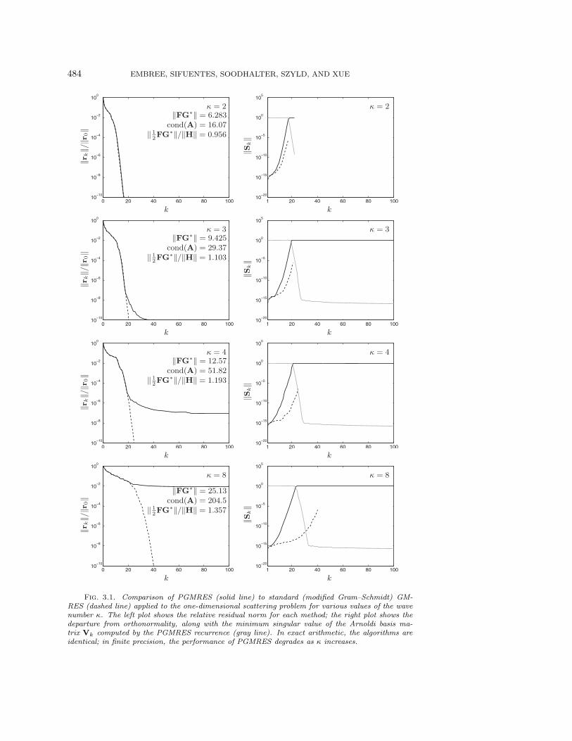
Figure 3.1 shows the convergence of the GMRES and PGMRES residuals forthe Lippmann–Schwinger problem (with a random b) for four choices of the wavenumber κ, all with constant m = −1 and discretization dimension n = 1000. Asthe wave number increases, the PGMRES residual curve departs from the standardGMRES curve, stagnating at increasingly large residuals. One might argue that theinstability is not significant at κ = 3; when κ = 8 the stagnation entirely compromisesthe utility of the algorithm.

To investigate the stagnation, we retain all Arnoldi vectors in PGMRES (in spiteof only using three at a time to compute the new iterate), and compute the departureof the computed Arnoldi basis from orthogonality, ‖(I+Uk)

−1Uk‖, at each iteration.The right plots in Figure 3.1 compare this loss of orthogonality for PGMRES to thatobserved for standard GMRES (with a full-length Arnoldi recurrence based on themodified Gram–Schmidt process). Both PGMRES and GMRES produce bases thatlose orthogonality, but GMRES does so at a slower pace that does not significantlydestabilize the convergence, consistent with the analysis of Greenbaum, Rozloznık,and Strakos [10]. Observe that the PGMRES residual departs from that producedby GMRES when the departure from orthogonality approaches one and the Arnoldivectors begin to approach linear dependence. (In section 4 we present an alternative


Fig. 3.1. Comparison of PGMRES (solid line) to standard (modified Gram–Schmidt) GM-RES (dashed line) applied to the one-dimensional scattering problem for various values of the wavenumber κ. The left plot shows the relative residual norm for each method; the right plot shows thedeparture from orthonormality, along with the minimum singular value of the Arnoldi basis ma-trix Vk computed by the PGMRES recurrence (gray line). In exact arithmetic, the algorithms areidentical; in finite precision, the performance of PGMRES degrades as κ increases.


method that applies MINRES to the Hermitian part of A. While it is well known thatthe Lanczos recurrence for computing an orthonormal basis for the Krylov subspacecan cause loss of orthogonality (see, e.g. [21]), this basis does not usually lose linearindependence, and the MINRES algorithm derived from this basis does not typicallyexhibit the early stagnation seen in some of the PGMRES examples here.)

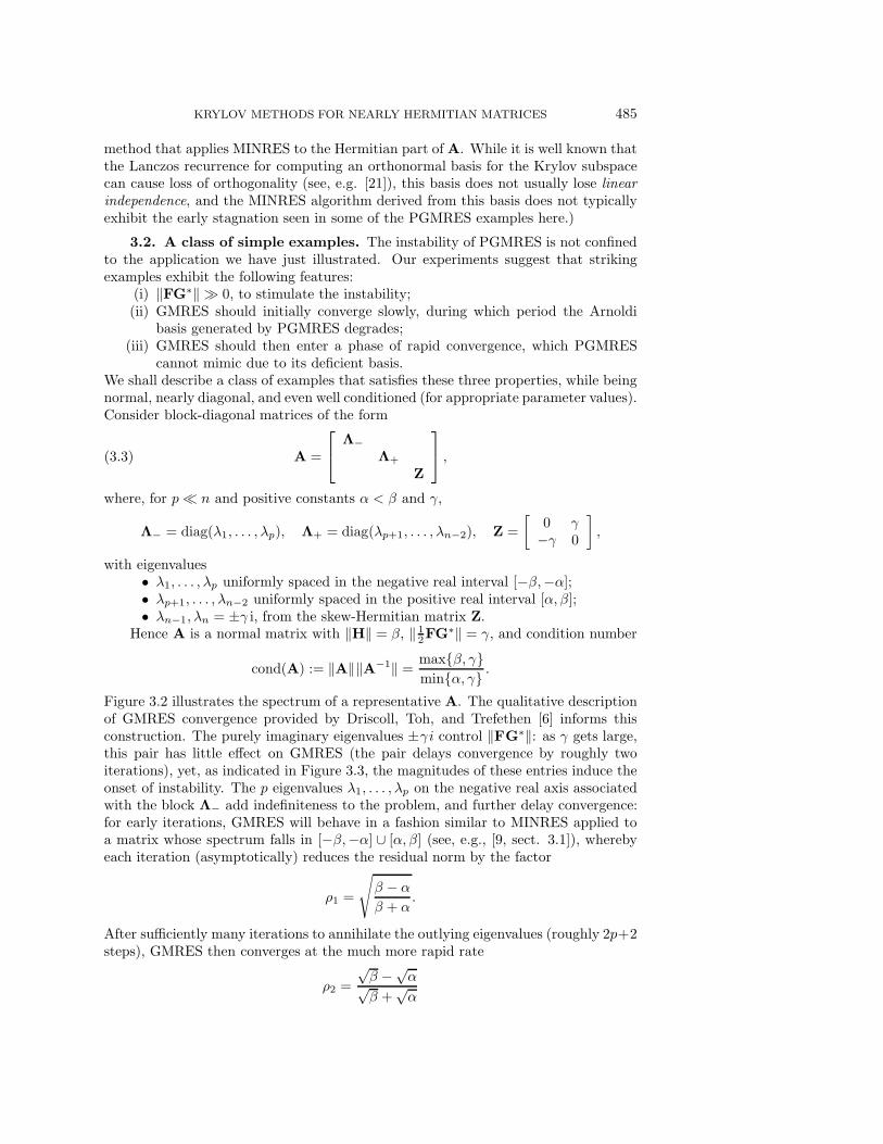
3.2. A class of simple examples. The instability of PGMRES is not confinedto the application we have just illustrated. Our experiments suggest that strikingexamples exhibit the following features:

(i) ‖FG∗‖ � 0, to stimulate the instability;(ii) GMRES should initially converge slowly, during which period the Arnoldi

basis generated by PGMRES degrades;(iii) GMRES should then enter a phase of rapid convergence, which PGMRES

cannot mimic due to its deficient basis.We shall describe a class of examples that satisfies these three properties, while beingnormal, nearly diagonal, and even well conditioned (for appropriate parameter values).Consider block-diagonal matrices of the form

(3.3) A =

⎡⎣ Λ−Λ+

Z

⎤⎦ ,

where, for p� n and positive constants α < β and γ,

Λ− = diag(λ1, . . . , λp), Λ+ = diag(λp+1, . . . , λn−2), Z =

[0 γ−γ 0

],

with eigenvalues• λ1, . . . , λp uniformly spaced in the negative real interval [−β,−α];• λp+1, . . . , λn−2 uniformly spaced in the positive real interval [α, β];• λn−1, λn = ±γ i, from the skew-Hermitian matrix Z.

Hence A is a normal matrix with ‖H‖ = β, ‖ 12FG∗‖ = γ, and condition number

cond(A) := ‖A‖‖A−1‖ = max{β, γ}min{α, γ} .

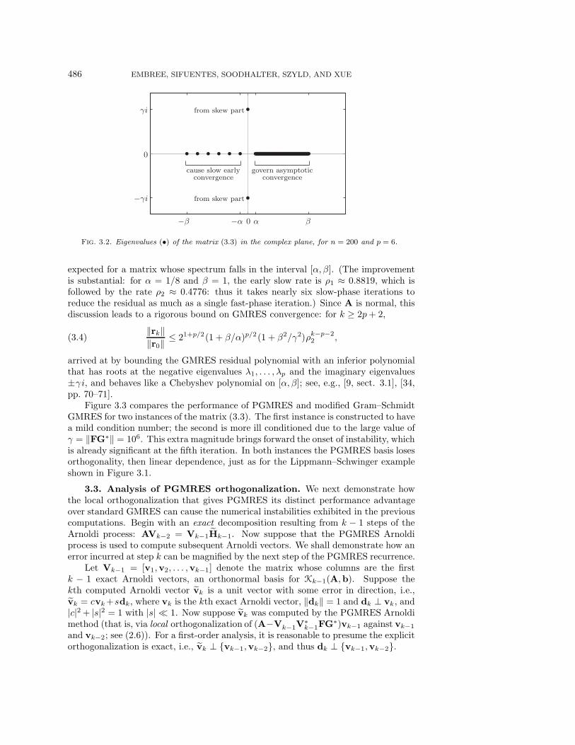
Figure 3.2 illustrates the spectrum of a representative A. The qualitative descriptionof GMRES convergence provided by Driscoll, Toh, and Trefethen [6] informs thisconstruction. The purely imaginary eigenvalues ±γi control ‖FG∗‖: as γ gets large,this pair has little effect on GMRES (the pair delays convergence by roughly twoiterations), yet, as indicated in Figure 3.3, the magnitudes of these entries induce theonset of instability. The p eigenvalues λ1, . . . , λp on the negative real axis associatedwith the block Λ− add indefiniteness to the problem, and further delay convergence:for early iterations, GMRES will behave in a fashion similar to MINRES applied toa matrix whose spectrum falls in [−β,−α] ∪ [α, β] (see, e.g., [9, sect. 3.1]), wherebyeach iteration (asymptotically) reduces the residual norm by the factor

ρ1 =

√β − α

β + α.

After sufficiently many iterations to annihilate the outlying eigenvalues (roughly 2p+2steps), GMRES then converges at the much more rapid rate

ρ2 =

√β −√α√β +√α


Fig. 3.2. Eigenvalues (•) of the matrix (3.3) in the complex plane, for n = 200 and p = 6.

expected for a matrix whose spectrum falls in the interval [α, β]. (The improvementis substantial: for α = 1/8 and β = 1, the early slow rate is ρ1 ≈ 0.8819, which isfollowed by the rate ρ2 ≈ 0.4776: thus it takes nearly six slow-phase iterations toreduce the residual as much as a single fast-phase iteration.) Since A is normal, thisdiscussion leads to a rigorous bound on GMRES convergence: for k ≥ 2p+ 2,

(3.4)‖rk‖‖r0‖ ≤ 21+p/2(1 + β/α)p/2 (1 + β2/γ2)ρk−p−2

2 ,

arrived at by bounding the GMRES residual polynomial with an inferior polynomialthat has roots at the negative eigenvalues λ1, . . . , λp and the imaginary eigenvalues±γi, and behaves like a Chebyshev polynomial on [α, β]; see, e.g., [9, sect. 3.1], [34,pp. 70–71].

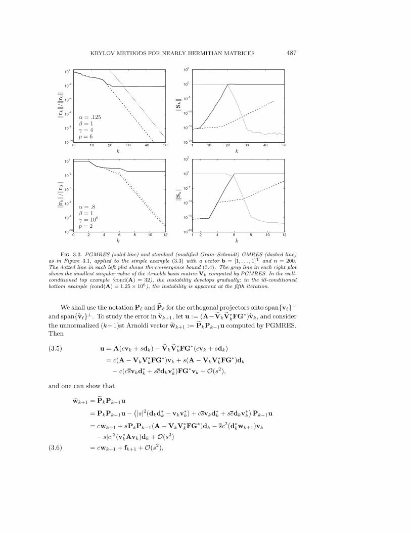
Figure 3.3 compares the performance of PGMRES and modified Gram–SchmidtGMRES for two instances of the matrix (3.3). The first instance is constructed to havea mild condition number; the second is more ill conditioned due to the large value ofγ = ‖FG∗‖ = 106. This extra magnitude brings forward the onset of instability, whichis already significant at the fifth iteration. In both instances the PGMRES basis losesorthogonality, then linear dependence, just as for the Lippmann–Schwinger exampleshown in Figure 3.1.

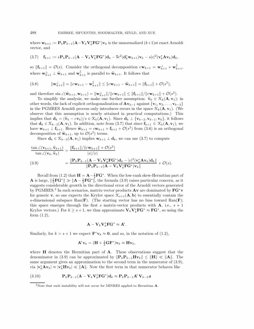
3.3. Analysis of PGMRES orthogonalization. We next demonstrate howthe local orthogonalization that gives PGMRES its distinct performance advantageover standard GMRES can cause the numerical instabilities exhibited in the previouscomputations. Begin with an exact decomposition resulting from k − 1 steps of theArnoldi process: AVk−2 = Vk−1Hk−1. Now suppose that the PGMRES Arnoldiprocess is used to compute subsequent Arnoldi vectors. We shall demonstrate how anerror incurred at step k can be magnified by the next step of the PGMRES recurrence.

Let Vk−1 = [v1,v2, . . . ,vk−1] denote the matrix whose columns are the firstk − 1 exact Arnoldi vectors, an orthonormal basis for Kk−1(A,b). Suppose thekth computed Arnoldi vector vk is a unit vector with some error in direction, i.e.,vk = cvk+sdk, where vk is the kth exact Arnoldi vector, ‖dk‖ = 1 and dk ⊥ vk, and|c|2 + |s|2 = 1 with |s| � 1. Now suppose vk was computed by the PGMRES Arnoldimethod (that is, via local orthogonalization of (A−Vk−1V

∗k−1FG

∗)vk−1 against vk−1

and vk−2; see (2.6)). For a first-order analysis, it is reasonable to presume the explicitorthogonalization is exact, i.e., vk ⊥ {vk−1,vk−2}, and thus dk ⊥ {vk−1,vk−2}.


Fig. 3.3. PGMRES (solid line) and standard (modified Gram–Schmidt) GMRES (dashed line)as in Figure 3.1, applied to the simple example (3.3) with a vector b = [1, . . . , 1]T and n = 200.The dotted line in each left plot shows the convergence bound (3.4). The gray line in each right plotshows the smallest singular value of the Arnoldi basis matrix Vk computed by PGMRES. In the well-conditioned top example (cond(A) = 32), the instability develops gradually; in the ill-conditionedbottom example (cond(A) = 1.25× 106), the instability is apparent at the fifth iteration.

We shall use the notation P� and P� for the orthogonal projectors onto span{v�}⊥and span{v�}⊥. To study the error in vk+1, let u := (A−VkV

∗kFG

∗)vk, and consider

the unnormalized (k+1)st Arnoldi vector wk+1 := PkPk−1u computed by PGMRES.Then

u = A(cvk + sdk)− VkV∗kFG

∗(cvk + sdk)(3.5)

= c(A−VkV∗kFG

∗)vk + s(A−VkV∗kFG

∗)dk

− c(csvkd∗k + scdkv

∗k)FG

∗vk +O(s2),

and one can show that

wk+1 = PkPk−1u

= PkPk−1u−(|s|2(dkd

∗k − vkv

∗k) + csvkd

∗k + scdkv

∗k

)Pk−1u

= cwk+1 + sPkPk−1(A−VkV∗kFG

∗)dk − sc2(d∗kwk+1)vk

− s|c|2(v∗kAvk)dk +O(s2)

= cwk+1 + fk+1 +O(s2),(3.6)


wherewk+1 := PkPk−1(A−VkV∗kFG

∗)vk is the unnormalized (k+1)st exact Arnoldivector, and

(3.7) fk+1 := sPkPk−1(A−VkV∗kFG

∗)dk − sc2(d∗kwk+1)vk − s|c|2(v∗

kAvk)dk,

so ‖fk+1‖ = O(s). Consider the orthogonal decomposition cwk+1 = w⊥k+1 + w

‖k+1,

where w⊥k+1 ⊥ wk+1 and w

‖k+1 is parallel to wk+1. It follows that

(3.8) ‖w⊥k+1‖ = ‖cwk+1 −w

‖k+1‖ ≤ ‖cwk+1 − wk+1‖ = ‖fk+1‖+O(s2),

and therefore sin∠(wk+1,wk+1) = ‖w⊥k+1‖/‖cwk+1‖ ≤ ‖fk+1‖/‖cwk+1‖+O(s2).

To simplify the analysis, we make one further assumption: vk ∈ Kk(A,v1); inother words, the lack of explicit orthogonalization ofAvk−1 against {v1,v2, . . . ,vk−3}in the PGMRES Arnoldi process only introduces errors in the space Kk(A,v1). (Weobserve that this assumption is nearly attained in practical computations.) Thisimplies that dk = (vk − cvk)/s ∈ Kk(A,v1). Since dk ⊥ {vk−2,vk−1,vk}, it followsthat dk ∈ Kk−3(A,v1). In addition, note from (3.7) that since fk+1 ∈ Kk(A,v1), wehave wk+1 ⊥ fk+1. Hence wk+1 = cwk+1 + fk+1 +O(s2) from (3.6) is an orthogonaldecomposition of wk+1, up to O(s2) terms.

Since dk ∈ Kk−3(A,v1) implies wk+1 ⊥ dk, we can use (3.7) to compute

tan∠(vk+1, vk+1)

tan∠(vk, vk)=‖fk+1‖/‖cwk+1‖+O(s2)

|s|/|c|

=‖PkPk−1(A−VkV

∗kFG

∗)dk − |c|2(v∗kAvk)dk‖

‖PkPk−1(A−VkV∗kFG

∗)vk‖ +O(s).(3.9)

Recall from (1.2) thatH = A− 12FG

∗. When the low-rank skew-Hermitian part ofA is large, ‖ 12FG∗‖ � ‖A− 1

2FG∗‖, the formula (3.9) raises particular concern, as it

suggests considerable growth in the directional error of the Arnoldi vectors generatedby PGMRES.2 In such scenarios, matrix-vector products Av are dominated by FG∗vfor generic v, so one expects the Krylov space Ks+1(A,b) to essentially contain thes-dimensional subspace Ran(F). (The starting vector has no bias toward Ran(F);this space emerges through the first s matrix-vector products with A, i.e., s + 1Krylov vectors.) For k ≥ s+1, we thus approximate VkV

∗kFG

∗ ≈ FG∗, so using theform (1.2),

A−VkV∗kFG

∗ ≈ A∗.

Similarly, for k > s+ 1 we expect F∗vk ≈ 0, and so, in the notation of (1.2),

A∗vk = (H+ 12GF∗)vk ≈ Hvk,

where H denotes the Hermitian part of A. These observations suggest that thedenominator in (3.9) can be approximated by ‖PkPk−1Hvk‖ ≤ ‖H‖ � ‖A‖. Thesame argument gives an approximation to the second term in the numerator of (3.9),via |v∗

kAvk| ≈ |v∗kHvk| � ‖A‖. Now the first term in that numerator behaves like

(3.10) PkPk−1(A−VkV∗kFG

∗)dk ≈ PkPk−1A∗Vk−3 z

2Note that such instability will not occur for MINRES applied to Hermitian A.


for some z ∈ Ck−3, since dk ∈ Kk−3(A,b). Presuming dk to arise from an arbi-trary perturbation, we expect (3.10) to be on the order of ‖A‖, so (3.9) will have alarge numerator and small denominator: for k > s + 1, we expect the kth iterationcan magnify the angular error in the PGMRES Arnoldi basis vector on the order of‖A‖/‖H‖. Indeed, in numerical experiments like those shown in Figures 3.1 and 3.3,increasing ‖FG∗‖ brings about earlier stagnation of PGMRES. Successful PGMREScomputations seem to require that FG∗ be small in both rank and norm.

In summary, the step that causes the loss of orthogonality in the PGMRESArnoldi procedure is the same step that makes PGMRES so computationally at-tractive, alleviating the need to preserve all Arnoldi basis vectors. In cases where theskew-Hermitian part of A is small in both rank and norm, and GMRES convergessteadily, our experience suggests that PGMRES can be viable; otherwise, numeri-cal instabilities often induce stagnation before convergence to a reasonable tolerance.Though we cannot propose a repair for this instability, in the next section we sug-gest an alternative method for efficiently solving a nearly Hermitian linear system.This method will have similar storage characteristics, but will avoid the numericalproblems endemic to PGMRES.

4. An alternative approach. We seek an efficient alternative method for solv-ing Ax = b when A has the “nearly Hermitian” form (1.2) that avoids the unstableperformance of PGMRES. Here we present such a method that requires only three-term recurrences. This algorithm follows from the simple observation that we canexpress nearly Hermitian matrices in the form

(4.1) A = H+ FCF∗,

where H := (A +A∗)/2, the Hermitian part of A, is assumed to be invertible, andFCF∗ = (A −A∗)/2 is a decomposition of the low-rank skew-Hermitian part, withC ∈ Cs×s skew-Hermitian and F ∈ Cn×s. For example, one can think of FCF∗ asa reduced unitary diagonalization of the skew-Hermitian part, or one can computeC from the representation (1.2) by solving FC∗ = 1

2G. Other decompositions mayfollow more naturally from the underlying mathematical model.

When the Hermitian part H is invertible, one can use it as a preconditioner, e.g.,

H−1A = I+H−1FCF∗.

A rank-s perturbation of the identity, this matrix will require no more than s+1 iter-ations of GMRES to reach convergence (provided H is nonsingular). The philosophybehind this preconditioner is the same as in the CGW method [4, 37], except that inthe latter, the Hermitian part needs to be positive definite; see also [15, Thm. 2.10]. Toform the preconditioned system, one can first compute H−1F and H−1b by solvings + 1 Hermitian linear systems for the same coefficient matrix H using the short-recurrence MINRES [20] or conjugate gradient [13] algorithms (possibly as a blockmethod, or in parallel). Inexact computation of the preconditioner can affect GMRESconvergence, as discussed in [27], [30, sect. 6], spoiling exact convergence. Here wedescribe an alternative strategy, based on the Schur complement, that requires thesolution of s + 1 systems with MINRES, followed by the solution of an s × s linearsystem; no GMRES iterations are necessary.

Note that (4.1) is the Schur complement of −C−1 in the matrix

Φ =

[H FF∗ −C−1

],


so solving Ax = b is equivalent to solving[H FF∗ −C−1

] [xy

]=

[b0

].(4.2)

Schur complement methods for solving systems of the form (4.2) are well known;see, e.g., [2, 5]. One such method eliminates x by inserting x = H−1(b − Fy) intoF∗x−C−1y = 0, and solving for y through the s-dimensional system

(4.3)(F∗H−1F+C−1

)y = F∗H−1b.

When the formulation (1.2) is more natural, this last equation takes the form

(4.4)(G∗H−1F+ 2I

)y = G∗H−1b.

This approach is equivalent to applying the Sherman–Morrison–Woodbury formulato (4.1); see, e.g., [12, 26, 38].

The solution of (1.1) via the method just described requires the solution of

(4.5) HW = F and Hu = b,

for W ∈ Cn×s and u ∈ Cn, as well as the s × s system (4.3) or (4.4) for y. Fromthese ingredients, one can construct x = u −Wy. This approach is described in amore general setting in, e.g., [12, 39].

Since H is Hermitian, one can approximate the solutions to (4.5) via a Krylovsubspace method driven by the three-term Lanczos recurrence. One can use MINRESor, for positive definite H, the conjugate gradient (CG) method. Thus, constructingan approximate solution to (1.1) requires s+1 Hermitian solves. Methods for solvinga Hermitian system with several right-hand sides (see, e.g., [11, 17, 24, 29]) couldpotentially expedite this calculation.

The decomposition of the skew-Hermitian part into FG∗ or FCF∗ is not unique,so one could, in principle, select the factorization in a way that optimizes the condi-tioning of the system in (4.3) or (4.4). For example, a result of Yip [39, Thm. 1] impliesthat some choice of F and G ensures that the condition number cond(G∗H−1F+2I)is bounded above by cond(A)cond(H).

We consider next the matter of choosing suitable stopping criteria for the Hermi-tian solves. For simplicity, assume henceforth in this section that F is scaled so that‖F‖ = 1, as is the case when F is derived from a reduced unitary diagonalization of

the skew-Hermitian part of A. Therefore ‖A − A∗‖/2 = ‖FCF∗‖ ≤ ‖C‖. Let Wand u denote approximate solutions to HW = F and Hu = b derived, e.g., fromMINRES. With these approximations in hand, one would replace (4.3) with the per-turbed s-dimensional system

(4.6) (F∗W +C−1)y = F∗u,

which can be solved directly with Gaussian elimination to yield the approximation

x = u− Wy

to the desired solution x. (For purposes of this analysis, we implicitly assume thatthis direct solve is computed exactly.) The residual of this approximation can beexpressed in terms of the other approximations:


r := b−Ax

= b− (H+ FCF∗)(u− Wy)

= b−Hu+HWy − FC(F∗u− F∗Wy)

= b−Hu+ (HW − F)y.

Basic norm inequalities yield a simple, dynamic stopping criterion.Theorem 4.1. Suppose A ∈ Cn×n is a nonsingular matrix of the form (4.1) with

‖F‖ ≤ 1 and nonsingular Hermitian part H. Let W and u be approximate solutions

to HW = F and Hu = b with residuals RW := F −HW and ru := b −Hu, andsuppose further that F∗W +C−1 is nonsingular. Then provided

‖RW‖‖y‖‖b‖ < ε/2 and

‖ru‖‖b‖ < ε/2,

and y exactly solves (4.6), then the approximate solution x := u− Wy satisfies

(4.7)‖b−Ax‖‖b‖ < ε.

Since y depends on W, the stopping criterion for W (i.e., ‖RW‖‖y‖/‖b‖ < ε/2)

in Theorem 4.1 cannot be expressed a priori. Once a candidate value for W has beenfound, one can solve the small s× s system (4.6) for y ∈ Cs, where s � n.3 With y

in hand, one can check if W satisfies the stopping criterion; if not, conduct furtherMINRES iterations to refine W, and test the criterion again with the updated y.

Adapting notation slightly, let W and W denote two approximate solutions toHW = F with corresponding solutions y and y to (4.6). The following result quanti-

fies the rate at which y→ y as W→ W, thus emphasizing that the dynamic stoppingcriterion supplied by Theorem 4.1 is stable with respect to refinements to W.

Theorem 4.2. Let y, y ∈ Cs solve the nonsingular linear systems

(F∗W +C−1)y = F∗u,

(F∗W +C−1)y = F∗u,

with ‖F‖ ≤ 1. Then for sufficiently small ‖W − W‖ and Ω := F∗W +C−1,

‖y − y‖ ≤ ‖Ω−1‖ ‖W − W‖ ‖y‖

1− ‖Ω−1‖ ‖W− W‖and

‖y‖ ≤ ‖y‖+ ‖Ω−1‖ ‖W − W‖ ‖y‖

1− ‖Ω−1‖ ‖W− W‖.

Proof. Since the difference between the coefficient matrix in solving for y and yis bounded in norm by ‖W− W‖, the result follows directly from basic perturbation

theory for linear systems [14, Thm. 7.2], provided ‖Ω−1‖ ‖W− W‖ < 1.

3In the case of the one-dimensional scattering problem in the last section, s = 2.


Recasting Ax = b into Hx + Fy = b and CF∗x = y expresses the right-handside vector b as the sum of vectors in Ran(H) and Ran(F). An a priori bound for‖y‖ or ‖y‖ would thus require knowledge of quantities such as ‖A−1‖ or ‖H−1‖,both of which are computationally prohibitive, particularly compared to the cost ofevaluating the dynamic bound in Theorem 4.1. We provide such a bound mainly fortheoretical interest.

Theorem 4.3. Suppose ‖F‖ ≤ 1, and that y and y solve

Ωy = F∗u, Ωy = F∗u

for nonsingular Ω := F∗W+C−1 and Ω := F∗W+C−1. If ‖H−1‖ ‖Ω−1‖ ‖RW‖ < 1,then

‖y‖ ≤ ‖Ω−1‖ ‖H−1‖( ‖b‖+ ‖ru‖1− ‖H−1‖ ‖Ω−1‖ ‖RW‖

),

where RW := F−HW and ru := b−Hu.Proof. The perturbation bound [14, Thm. 7.2] implies that

‖y‖ ≤ ‖y‖ + ‖y− y‖

≤ ‖y‖ + ‖H−1‖ ‖Ω−1‖1− ‖H−1‖ ‖Ω−1‖ ‖RW‖ (‖ru‖+ ‖RW‖ ‖y‖) ,(4.8)

since ‖Ω − Ω‖ ≤ ‖H−1‖ ‖RW‖ and ‖F∗u − F∗u‖ ≤ ‖H−1‖ ‖ru‖. The fact thaty = Ω−1F∗u = Ω−1F∗H−1b implies ‖y‖ ≤ ‖Ω−1‖ ‖H−1‖ ‖b‖, from which follows

‖y‖ ≤ ‖Ω−1‖ ‖H−1‖(‖b‖+ ‖ru‖+ ‖Ω

−1‖ ‖RW‖ ‖H−1‖ ‖b‖1− ‖H−1‖ ‖Ω−1‖ ‖RW‖

)= ‖Ω−1‖ ‖H−1‖

( ‖b‖+ ‖ru‖1− ‖H−1‖ ‖Ω−1‖ ‖RW‖

).

Corollary 4.4. Provided the approximate solutions u and W are sufficientlyaccurate that

‖ru‖‖b‖ ≤

ε

2and ‖RW‖ ≤ ε

‖Ω−1‖ ‖H−1‖(2 + 2ε),

the relative residual satisfies ‖r‖/‖b‖ < ε.We emphasize that the quantity ‖Ω−1‖ in the hypothesis and bound renders this

result inapplicable a priori, since Ω is a function of W. Approximating the value‖Ω−1‖ from W could give a dynamic estimate. Note that given an approximation

W, one can directly compute ‖y‖.The Schur complement method for solving nearly Hermitian linear systems is

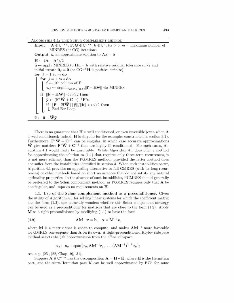
summarized in Algorithm 4.1, which uses the dynamic stopping criterion. Since thisconvergence test involves y, which requires an approximation to W, MINRES isapplied to the problems Hwj = fj for j = 1, . . . , s concurrently. Lines 8 through 10 ofthe algorithm can be replaced by a step-by-step block MINRES [17]. (Block methodsfor multiple right-hand sides can potentially give more rapid convergence than theaggregate cost of solving the systems one at a time [11, 17].) Also observe that itis not necessary to build the matrix H; one need only compute the matrix-vectorproduct Hx for a vector x.


Algorithm 4.1: The Schur complement method

Input : A ∈ Cn×n, F,G ∈ Cn×s, b ∈ Cn, tol > 0, m = maximum number ofMINRES (or CG) iterations

Output: x, an approximate solution to Ax = b

H← (A+A∗)/2u← apply MINRES to Hu = b with relative residual tolerance tol/2 andinitial iterate u0 = 0 (or CG if H is positive definite)for k = 1 to m do

for j = 1 to s dof ← jth column of Fwj ← argminw∈Kk(H,f)‖f −Hw‖ via MINRES

if ‖F−HW‖ < tol/2 then

y← (F∗W +C−1)−1F∗uif ‖F−HW‖ ‖y‖/‖b‖ < tol/2 then

End For Loop

x← u− Wy

There is no guarantee that H is well conditioned, or even invertible (even when Ais well conditioned: indeed, H is singular for the examples constructed in section 3.2).Furthermore, F∗W + C−1 can be singular, in which case accurate approximationsW give matrices F∗W + C−1 that are highly ill conditioned. For such cases, Al-gorithm 4.1 would likely be unsuitable. While Algorithm 4.1 does offer a methodfor approximating the solution to (1.1) that requires only three-term recurrences, itis not more efficient than the PGMRES method, provided the latter method doesnot suffer from the instabilities identified in section 3. When such instabilities occur,Algorithm 4.1 provides an appealing alternative to full GMRES (with its long recur-rences) or other methods based on short recurrences that do not satisfy any naturaloptimality properties. In the absence of such instabilities, PGMRES should generallybe preferred to the Schur complement method, as PGMRES requires only that A benonsingular, and imposes no requirements on H.

4.1. Use of the Schur complement method as a preconditioner. Giventhe utility of Algorithm 4.1 for solving linear systems for which the coefficient matrixhas the form (1.2), one naturally wonders whether this Schur complement strategycan be used as a preconditioner for matrices that are close to the form (1.2). ApplyM as a right preconditioner by modifying (1.1) to have the form

(4.9) AM−1z = b, x = M−1z,

where M is a matrix that is cheap to compute, and makes AM−1 more favorablefor GMRES convergence than A on its own. A right-preconditioned Krylov subspacemethod selects the jth approximation from the affine subspace

xj ∈ x0 + span{r0,AM−1r0, . . . ,

(AM−1

)j−1r0};

see, e.g., [25], [22, Chap. 9], [31].Suppose A ∈ Cn×n has the decomposition A = H+K, where H is the Hermitian

part, and the skew-Hermitian part K can be well approximated by FG∗ for some


F,G ∈ Cn×s with s � n, e.g., K = FG∗ + E with ‖E‖ � 1. Systems such asthis arise, for example, in discretizations of PDEs with certain Neuman boundaryconditions, or more generically when K has a small number of dominant singularvalues. In such instances, we expect M = H+FG∗ to be an effective preconditionerfor A, while allowing for rapid application through Algorithm 4.1.

Recall that Algorithm 4.1 requires s + 1 applications of MINRES, which couldbe prohibitive to apply at each iteration of GMRES applied to the preconditionedsystem. However, s of these applications are needed to solve HW = F; the solutionof this system can be computed once and reused at each GMRES iteration. Using vj

here to denote the jth Arnoldi vector in the (outer) preconditioned GMRES iteration,each preconditioner applicationM−1vj will require only the solution of one Hermitiansystem, Hx = vj , and the direct solution of one s×s system. Thus this preconditioneris relatively cheap to compute at each step, after the up-front cost of solvingHW = F.

5. Numerical results. To demonstrate the effectiveness of the proposed Schurcomplement approach, we apply Algorithm 4.1 to several problems. To put this newalgorithm in context, we also solve our linear system using MATLAB’s full GMRESalgorithm [16] and the recently proposed IDR(2) method [32, 33], as implementedby van Gijzen [36]. The IDR(2) method is a modern short recurrence method thatuses right and left Krylov subspaces. In the numerical examples in this section, theSchur complement method is implemented using the MINRES algorithm describedin [7, sect. 6.5] (which has a similar level of overhead as the PGMRES and IDRimplementations we use). In most of our experiments we apply the MINRES runsin series, but the Schur complement algorithm allows for easy parallelization of thesecalls, since each MINRES run can be done independently. In fact, we show oneparallel numerical experiment in section 5.3. When PGMRES is successful, it is oftenthe most efficient algorithm. (Except for the parallel computations in section 5.3, allexperiments were run on a MacBook Pro with a 2.66 GHz Intel Core i7 processor and4GB of DDR3 dynamic RAM.)

5.1. Simple example, revisited. In section 3.2, we introduced a simple, well-conditioned matrix (3.3) with a skew-Hermitian part of low rank. The analysis pre-sented in section 3.3 suggests that as the norm of the skew-Hermitian part grows, thenumerical instability of PGMRES causes the residual to stagnate earlier. To applyAlgorithm 4.1, however, we require that the Hermitian part of A be nonsingular; thusfor the tests in this section, we modify (3.3) by adding a 2× 2 identity to the Z block(thus shifting the zero eigenvalues of the Hermitian part to one). As is clear fromFigure 5.1, this does not change the convergence behavior discussed in section 3.2. Itfollows from Theorem 4.1 that

(5.1) γk := ‖rb,k‖+√2‖y‖(‖rf1,k‖+ ‖rf2,k‖)

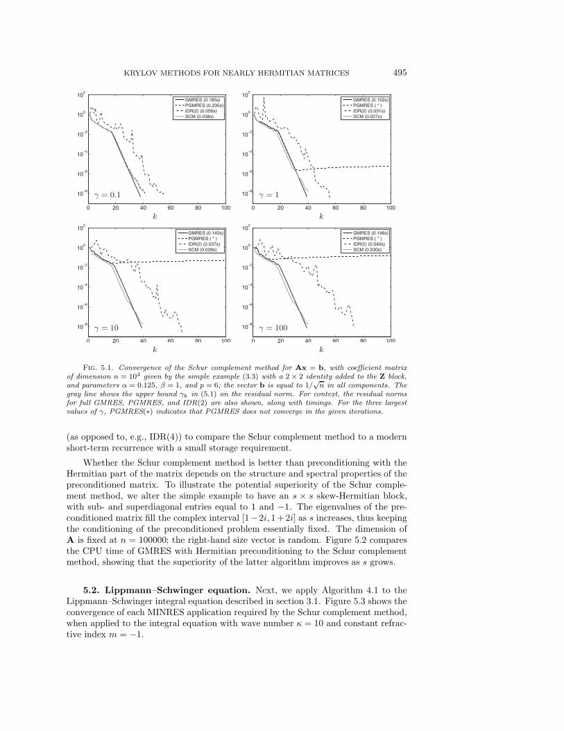
is an upper bound on the norm of the residual produced at each iteration of the Schurcomplement method. The vectors rb,k, rf1,k, and rf2,k are the residuals produced byMINRES with coefficient matrix H = (A+A∗)/2 and right-hand sides b, f1, and f2.To simplify the illustration of our numerical results in Figure 5.1, we plot γk versusk for the Schur complement approach. Observe that this method is superior in runtime to full GMRES, PGMRES, and IDR(2), and competitive or superior in iterationcount as well. (Note that γk can be smaller than the full GMRES residual norm,since the Schur complement method does not draw its approximations from the sameKrylov subspace from which GMRES draws its optimal iterates.) We chose IDR(2)


Fig. 5.1. Convergence of the Schur complement method for Ax = b, with coefficient matrixof dimension n = 104 given by the simple example (3.3) with a 2× 2 identity added to the Z block,and parameters α = 0.125, β = 1, and p = 6; the vector b is equal to 1/

√n in all components. The

gray line shows the upper bound γk in (5.1) on the residual norm. For context, the residual normsfor full GMRES, PGMRES, and IDR(2) are also shown, along with timings. For the three largestvalues of γ, PGMRES(∗) indicates that PGMRES does not converge in the given iterations.

(as opposed to, e.g., IDR(4)) to compare the Schur complement method to a modernshort-term recurrence with a small storage requirement.

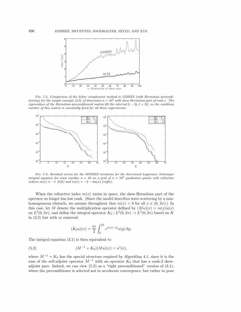
Whether the Schur complement method is better than preconditioning with theHermitian part of the matrix depends on the structure and spectral properties of thepreconditioned matrix. To illustrate the potential superiority of the Schur comple-ment method, we alter the simple example to have an s × s skew-Hermitian block,with sub- and superdiagonal entries equal to 1 and −1. The eigenvalues of the pre-conditioned matrix fill the complex interval [1− 2i, 1+2i] as s increases, thus keepingthe conditioning of the preconditioned problem essentially fixed. The dimension ofA is fixed at n = 100000; the right-hand size vector is random. Figure 5.2 comparesthe CPU time of GMRES with Hermitian preconditioning to the Schur complementmethod, showing that the superiority of the latter algorithm improves as s grows.

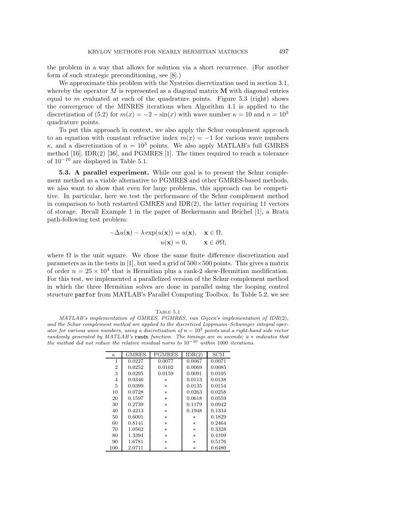
5.2. Lippmann–Schwinger equation. Next, we apply Algorithm 4.1 to theLippmann–Schwinger integral equation described in section 3.1. Figure 5.3 shows theconvergence of each MINRES application required by the Schur complement method,when applied to the integral equation with wave number κ = 10 and constant refrac-tive index m = −1.


Fig. 5.2. Comparison of the Schur complement method to GMRES (with Hermitian precondi-tioning) for the simple example (3.3) of dimension n = 105 with skew-Hermitian part of rank s. Theeigenvalues of the Hermitian-preconditioned matrix fill the interval [1− 2i, 1 + 2i], so the conditionnumber of this matrix is essentially fixed for all these experiments.

Fig. 5.3. Residual norms for the MINRES iterations for the discretized Lippmann–Schwingerintegral equation for wave number κ = 10 on a grid of n = 103 quadrature points with refractiveindices m(x) ≡ −1 (left) and m(x) = −2− sin(x) (right).

When the refractive index m(x) varies in space, the skew-Hermitian part of theoperator no longer has low rank. (Since the model describes wave scattering by a non-homogeneous obstacle, we assume throughout that m(x) < 0 for all x ∈ (0, 2π).) Inthis case, let M denote the multiplication operator defined by (Mu)(x) = m(x)u(x)on L2(0, 2π), and define the integral operator K0 : L2(0, 2π)→ L2(0, 2π) based on Kin (3.2) but with m removed:

(K0u)(x) =iκ

2

∫ 2π

0

eiκ|x−y|u(y) dy.

The integral equation (3.1) is then equivalent to

(5.2) (M−1 +K0)(Mu)(x) = ui(x),

where M−1 +K0 has the special structure required by Algorithm 4.1, since it is thesum of the self-adjoint operator M−1 with an operator K0 that has a rank-2 skew-adjoint part. Indeed, we can view (5.2) as a “right preconditioned” version of (3.1),where the preconditioner is selected not to accelerate convergence, but rather to pose


the problem in a way that allows for solution via a short recurrence. (For anotherform of such strategic preconditioning, see [8].)

We approximate this problem with the Nystrom discretization used in section 3.1,whereby the operator M is represented as a diagonal matrix M with diagonal entriesequal to m evaluated at each of the quadrature points. Figure 5.3 (right) showsthe convergence of the MINRES iterations when Algorithm 4.1 is applied to thediscretization of (5.2) for m(x) = −2− sin(x) with wave number κ = 10 and n = 103

quadrature points.To put this approach in context, we also apply the Schur complement approach

to an equation with constant refractive index m(x) = −1 for various wave numbersκ, and a discretization of n = 103 points. We also apply MATLAB’s full GMRESmethod [16], IDR(2) [36], and PGMRES [1]. The times required to reach a toleranceof 10−10 are displayed in Table 5.1.

5.3. A parallel experiment. While our goal is to present the Schur comple-ment method as a viable alternative to PGMRES and other GMRES-based methods,we also want to show that even for large problems, this approach can be competi-tive. In particular, here we test the performance of the Schur complement methodin comparison to both restarted GMRES and IDR(2), the latter requiring 11 vectorsof storage. Recall Example 1 in the paper of Beckermann and Reichel [1], a Bratupath-following test problem:

−Δu(x)− λ exp(u(x)) = u(x), x ∈ Ω,

u(x) = 0, x ∈ ∂Ω,

where Ω is the unit square. We chose the same finite difference discretization andparameters as in the tests in [1], but used a grid of 500×500 points. This gives a matrixof order n = 25 × 104 that is Hermitian plus a rank-2 skew-Hermitian modification.For this test, we implemented a parallelized version of the Schur complement methodin which the three Hermitian solves are done in parallel using the looping controlstructure parfor from MATLAB’s Parallel Computing Toolbox. In Table 5.2, we see

Table 5.1

MATLAB’s implementation of GMRES, PGMRES, van Gijzen’s implementation of IDR(2),and the Schur complement method are applied to the discretized Lippmann–Schwinger integral oper-ator for various wave numbers, using a discretization of n = 103 points and a right-hand side vectorrandomly generated by MATLAB’s randn function. The timings are in seconds; a ∗ indicates thatthe method did not reduce the relative residual norm to 10−10 within 1000 iterations.

κ GMRES PGMRES IDR(2) SCM1 0.0227 0.0077 0.0067 0.00712 0.0252 0.0102 0.0069 0.00853 0.0295 0.0159 0.0091 0.01054 0.0346 ∗ 0.0113 0.01385 0.0399 ∗ 0.0135 0.0154

10 0.0728 ∗ 0.0263 0.025820 0.1597 ∗ 0.0618 0.055930 0.2739 ∗ 0.1179 0.094240 0.4213 ∗ 0.1948 0.133450 0.6001 ∗ ∗ 0.182960 0.8141 ∗ ∗ 0.246470 1.0562 ∗ ∗ 0.332880 1.3394 ∗ ∗ 0.410990 1.6781 ∗ ∗ 0.5176

100 2.0711 ∗ ∗ 0.6480


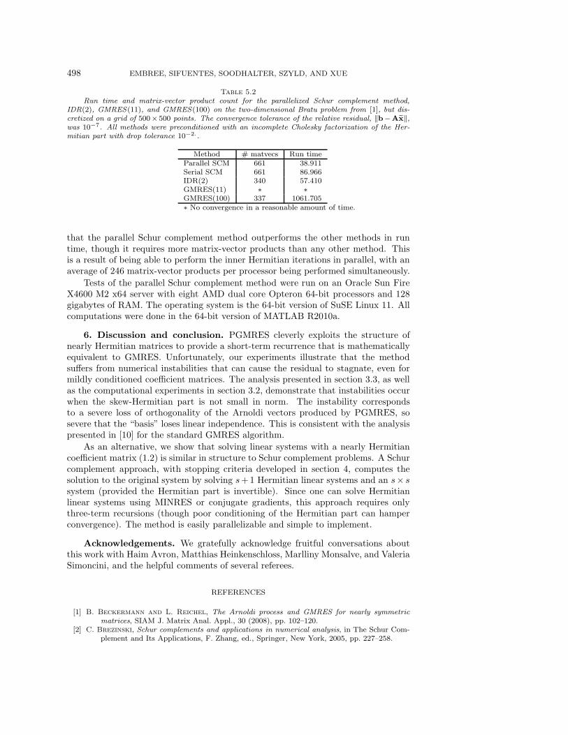
Table 5.2

Run time and matrix-vector product count for the parallelized Schur complement method,IDR(2), GMRES(11), and GMRES(100) on the two-dimensional Bratu problem from [1], but dis-cretized on a grid of 500× 500 points. The convergence tolerance of the relative residual, ‖b−Ax‖,was 10−7. All methods were preconditioned with an incomplete Cholesky factorization of the Her-mitian part with drop tolerance 10−2..

Method # matvecs Run timeParallel SCM 661 38.911Serial SCM 661 86.966IDR(2) 340 57.410GMRES(11) ∗ ∗GMRES(100) 337 1061.705∗ No convergence in a reasonable amount of time.

that the parallel Schur complement method outperforms the other methods in runtime, though it requires more matrix-vector products than any other method. Thisis a result of being able to perform the inner Hermitian iterations in parallel, with anaverage of 246 matrix-vector products per processor being performed simultaneously.

Tests of the parallel Schur complement method were run on an Oracle Sun FireX4600 M2 x64 server with eight AMD dual core Opteron 64-bit processors and 128gigabytes of RAM. The operating system is the 64-bit version of SuSE Linux 11. Allcomputations were done in the 64-bit version of MATLAB R2010a.

6. Discussion and conclusion. PGMRES cleverly exploits the structure ofnearly Hermitian matrices to provide a short-term recurrence that is mathematicallyequivalent to GMRES. Unfortunately, our experiments illustrate that the methodsuffers from numerical instabilities that can cause the residual to stagnate, even formildly conditioned coefficient matrices. The analysis presented in section 3.3, as wellas the computational experiments in section 3.2, demonstrate that instabilities occurwhen the skew-Hermitian part is not small in norm. The instability correspondsto a severe loss of orthogonality of the Arnoldi vectors produced by PGMRES, sosevere that the “basis” loses linear independence. This is consistent with the analysispresented in [10] for the standard GMRES algorithm.

As an alternative, we show that solving linear systems with a nearly Hermitiancoefficient matrix (1.2) is similar in structure to Schur complement problems. A Schurcomplement approach, with stopping criteria developed in section 4, computes thesolution to the original system by solving s+1 Hermitian linear systems and an s× ssystem (provided the Hermitian part is invertible). Since one can solve Hermitianlinear systems using MINRES or conjugate gradients, this approach requires onlythree-term recursions (though poor conditioning of the Hermitian part can hamperconvergence). The method is easily parallelizable and simple to implement.

Acknowledgements. We gratefully acknowledge fruitful conversations aboutthis work with Haim Avron, Matthias Heinkenschloss, Marlliny Monsalve, and ValeriaSimoncini, and the helpful comments of several referees.

REFERENCES

[1] B. Beckermann and L. Reichel, The Arnoldi process and GMRES for nearly symmetricmatrices, SIAM J. Matrix Anal. Appl., 30 (2008), pp. 102–120.

[2] C. Brezinski, Schur complements and applications in numerical analysis, in The Schur Com-plement and Its Applications, F. Zhang, ed., Springer, New York, 2005, pp. 227–258.


[3] Y. Chen and V. Rokhlin, On the inverse scattering problem for the Helmholtz equation inone dimension, Inverse Problems, 8 (1992), pp. 365–391.

[4] P. Concus and G. H. Golub, A generalized conjugate gradient method for nonsymmetricsystems of linear equations, in Computing Methods in Applied Sciences and Engineering,Part I, Lecture Notes in Econom. and Math. Systems, Springer, Berlin, 134 (1976), pp. 56–65.

[5] R. W. Cottle, Manifestations of the Schur complement, Linear Algebra Appl., 8 (1974),pp. 189–211.

[6] T. A. Driscoll, K.-C. Toh, and L. N. Trefethen, From potential theory to matrix iterationsin six steps, SIAM Rev., 40 (1998), pp. 547–578.

[7] B. Fischer, Polynomial Based Iteration Methods for Symmetric Linear Systems, Wiley–Teubner, Chichester, UK, 1996.

[8] B. Fischer, A. Ramage, D. J. Silvester, and A. J. Wathen, Minimum residual methods foraugmented systems, BIT, 38 (1998), pp. 527–543.

[9] A. Greenbaum, Iterative Methods for Solving Linear Systems, SIAM, Philadelphia, 1997.[10] A. Greenbaum, M. Rozloznık, and Z. Strakos, Numerical behaviour of the modified Gram–

Schmidt GMRES implementation, BIT, 37 (1997), pp. 706–719.[11] M. H. Gutknecht, Block Krylov space methods for linear systems with multiple right-hand

sides: an introduction, in Modern Mathematical Models, Methods and Algorithms for RealWorld Systems, A. H. Siddiqi, I. S. Duff, and O. Christensen, eds., Anamaya Publishers,New Delhi, 2007, pp. 420–447.

[12] W. W. Hager, Updating the inverse of a matrix, SIAM Rev., 31 (1989), pp. 221–239.[13] M. R. Hestenes and E. Stiefel, Methods of conjugate gradients for solving linear systems,

J. Research Nat. Bur. Standards, 49 (1952), pp. 409–436.[14] N. J. Higham, Accuracy and Stability of Numerical Algorithms, 2nd ed., SIAM, Philadelphia,

2002.[15] M. Huhtanen, A matrix nearness problem related to iterative methods, SIAM J. Numer. Anal.,

39 (2001), pp. 407–422.[16] MathWorks, MATLAB 2010a, Natick, MA, 2010.[17] D. P. O’Leary, The block conjugate gradient algorithm and related methods, Linear Algebra

Appl., 29 (1980), pp. 293–322.[18] C. C. Paige, A useful form of unitary matrix obtained from any sequence of unit 2-norm

n-vectors, SIAM J. Matrix Anal. Appl., 31 (2009), pp. 565–583.[19] C. C. Paige, M. Rozloznık, and Z. Strakos, Modified Gram–Schmidt (MGS), least squares,

and backward stability of MGS-GMRES, SIAM J. Matrix Anal. Appl., 28 (2006), pp. 264–284.

[20] C. C. Paige and M. A. Saunders, Solution of sparse indefinite systems of linear equations,SIAM J. Numer. Anal., 12 (1975), pp. 617–629.

[21] B. N. Parlett, The Symmetric Eigenvalue Problem, SIAM, Philadelphia, 1997.[22] Y. Saad, Iterative Methods for Sparse Linear Systems, 2nd ed., SIAM, Philadelphia, 2003.[23] Y. Saad and M. H. Schultz, GMRES: A generalized minimal residual algorithm for solving

nonsymmetric linear systems, SIAM J. Sci. Statist. Comput., 7 (1986), pp. 856–869.[24] Y. Saad, On the Lanczos method for solving symmetric linear systems with several right-hand

sides, Math. Comp., 48 (1987), pp. 651–662.[25] Y. Saad, A flexible inner-outer preconditioned GMRES algorithm, SIAM J. Sci. Comput., 14

(1993), pp. 461–469.[26] J. Sherman and W. J. Morrison, Adjustment of an inverse matrix corresponding to a change

in one element of a given matrix, Ann. Math. Statistics, 21 (1950), pp. 124–127.[27] J. A. Sifuentes, M. Embree, and R. B. Morgan, The Stability of GMRES Convergence,

with Application to Preconditioning by Approximate Deflation, Technical Report TR 11-12, Rice University, Department of Computational and Applied Mathematics, Houston,TX, 2011.

[28] J. Sifuentes, Preconditioned Iterative Methods for Inhomogeneous Acoustic Scattering Appli-cations, Ph.D. thesis, Rice University, Houston, TX, 2010.

[29] V. Simoncini and E. Gallopoulos, Convergence properties of block GMRES and matrixpolynomials, Linear Algebra Appl., 247 (1996), pp. 97–119.

[30] V. Simoncini and D. B. Szyld, On the occurrence of superlinear convergence of exact andinexact Krylov subspace methods, SIAM Rev., 47 (2005), pp. 247–272.

[31] V. Simoncini and D. B. Szyld, Recent computational developments in Krylov subspace meth-ods for linear systems, Numer. Linear Algebra Appl., 14 (2007), pp. 1–59.

[32] V. Simoncini and D. B. Szyld, Interpreting IDR as a Petrov–Galerkin method., SIAM J. Sci.Comput., 32 (2010), pp. 1898–1912.


[33] P. Sonneveld and M. B. van Gijzen, IDR(s): A family of simple and fast algorithms forsolving large nonsymmetric systems of linear equations, SIAM J. Sci. Comput., 31 (2008),pp. 1035–1062.

[34] D. B. Szyld and O. B. Widlund, Variational analysis of some conjugate gradient methods,East-West J. Numer. Math., 1 (1993), pp. 51–74.

[35] R. Vandebril and G. M. Del Corso, An implicit multishift QR-algorithm for Hermitian pluslow rank matrices, SIAM J. Sci. Comput., 32 (2010), pp. 2190–2212.

[36] M. B. van Gijzen, The Induced Dimension Reduction Method, 2010. Available athttp://ta.twi.tudelft.nl/nw/users/gijzen/IDR.html.

[37] O. B. Widlund, A Lanczos method for a class of nonsymmetric systems of linear equations,SIAM J. Numer. Anal., 15 (1978), pp. 801–812.

[38] M. A. Woodbury, Inverting Modified Matrices, Statistical Research Group, Memo. Rep. no.42, Princeton University, Princeton, NJ, 1950.

[39] E. L. Yip, A note on the stability of solving a rank-p modification of a linear system by theSherman–Morrison–Woodbury formula, SIAM J. Sci. Statist. Comput., 7 (1986), pp. 507–513.

SHORT-TERM RECURRENCE KRYLOV SUBSPACE METHODS

Documents

Transcript of SHORT-TERM RECURRENCE KRYLOV SUBSPACE METHODS