KRYLOV SUBSPACE ITERATION

Presented by: Nab Raj Roshyara

Master and Ph.D. StudentSupervisors:

Prof. Dr. Peter Benner,Department of Mathematics, TU Chemnitz

and

Dipl.-Geophys. Thomas Gunther

1. Februar 2005

1 Introductory part

1.1 What is an iterative method and why is it useful?

• All the numerical methods can be divided into two broad categories.

1. Direct methods:A direct method is one that produces the result in a prescribed,finite number of steps.e.g. All versions of Gaussian elimination for solving

Ax = b (1)

where A is n × n and non-singular, are direct methods.

2. Iterative methods(Indirect methods):Iterative methods are in contrast to direct methods. An iterativemethod is an attempt to solve a problem, for example an equationor system of equations, by finding successive approximations tothe solution starting from an initial guess.

• The answer of the question “why is iterative method useful?” is contai-ned in the following questions.

1

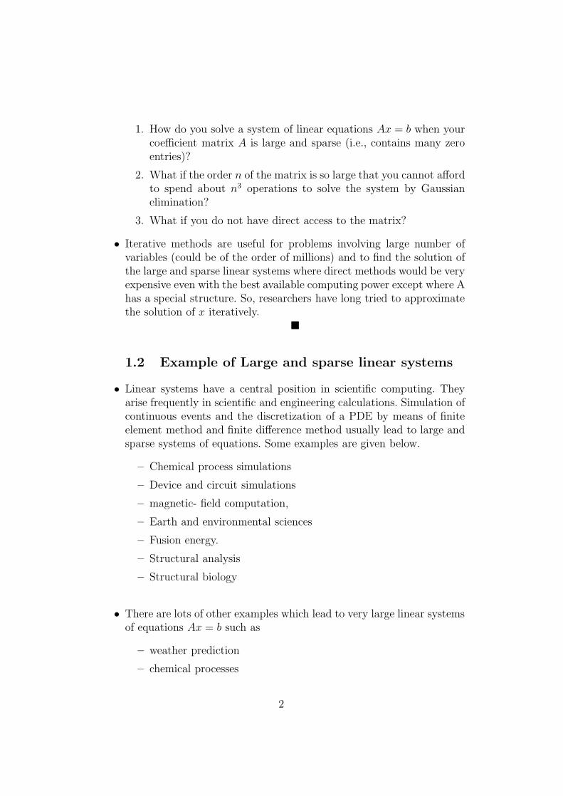
1. How do you solve a system of linear equations Ax = b when yourcoefficient matrix A is large and sparse (i.e., contains many zeroentries)?

2. What if the order n of the matrix is so large that you cannot affordto spend about n3 operations to solve the system by Gaussianelimination?

3. What if you do not have direct access to the matrix?

• Iterative methods are useful for problems involving large number ofvariables (could be of the order of millions) and to find the solution ofthe large and sparse linear systems where direct methods would be veryexpensive even with the best available computing power except where Ahas a special structure. So, researchers have long tried to approximatethe solution of x iteratively.

�

1.2 Example of Large and sparse linear systems

• Linear systems have a central position in scientific computing. Theyarise frequently in scientific and engineering calculations. Simulation ofcontinuous events and the discretization of a PDE by means of finiteelement method and finite difference method usually lead to large andsparse systems of equations. Some examples are given below.

– Chemical process simulations

– Device and circuit simulations

– magnetic- field computation,

– Earth and environmental sciences

– Fusion energy.

– Structural analysis

– Structural biology

• There are lots of other examples which lead to very large linear systemsof equations Ax = b such as

– weather prediction

– chemical processes

2

– semiconductor-device simulation

– nuclear-reactor safety problems

– mechanical- structure stress

– and so on.�

1.3 Basic idea of iterative method

• To find the solution x of the linear system (1), all iterative methodsrequire an initial guess x0 ∈ Rn that approximate the true solution. So,we start with a good guess x0 which can be taken by solving a mucheasier and similar problem.

• Once we have x0, we use it to generate a new guess x1 which is usedto guess x2 and so on. Moreover, we attempt to improve this guess byreducing the error with a convenient and cheap approximation.

• Let K be n×n be a simpler matrix which is similar to matrix A of theequation Ax = b. Thenin step i + 1 :we get a relation as follows:

Kxi+1 = Kxi + b − Axi (2)

From above equation (2), we solve the new approximation xi+1 for thesolution x of Ax = b.

• Remarks

1. The arbitrary initial start x0 converges if the modulus of largesteigen value of the matrix (I − K−1)A is less than 1.

2. It is difficult to explain exactly about the choice of the similarmatrix K of (2) but normally one can take

K = diag(A)

For example, to solve the discretized Poisson equation, the choiceK = diag(A) leads to a convergence rate 1− 0(h2) where h is thedistance between grid points.

�

3

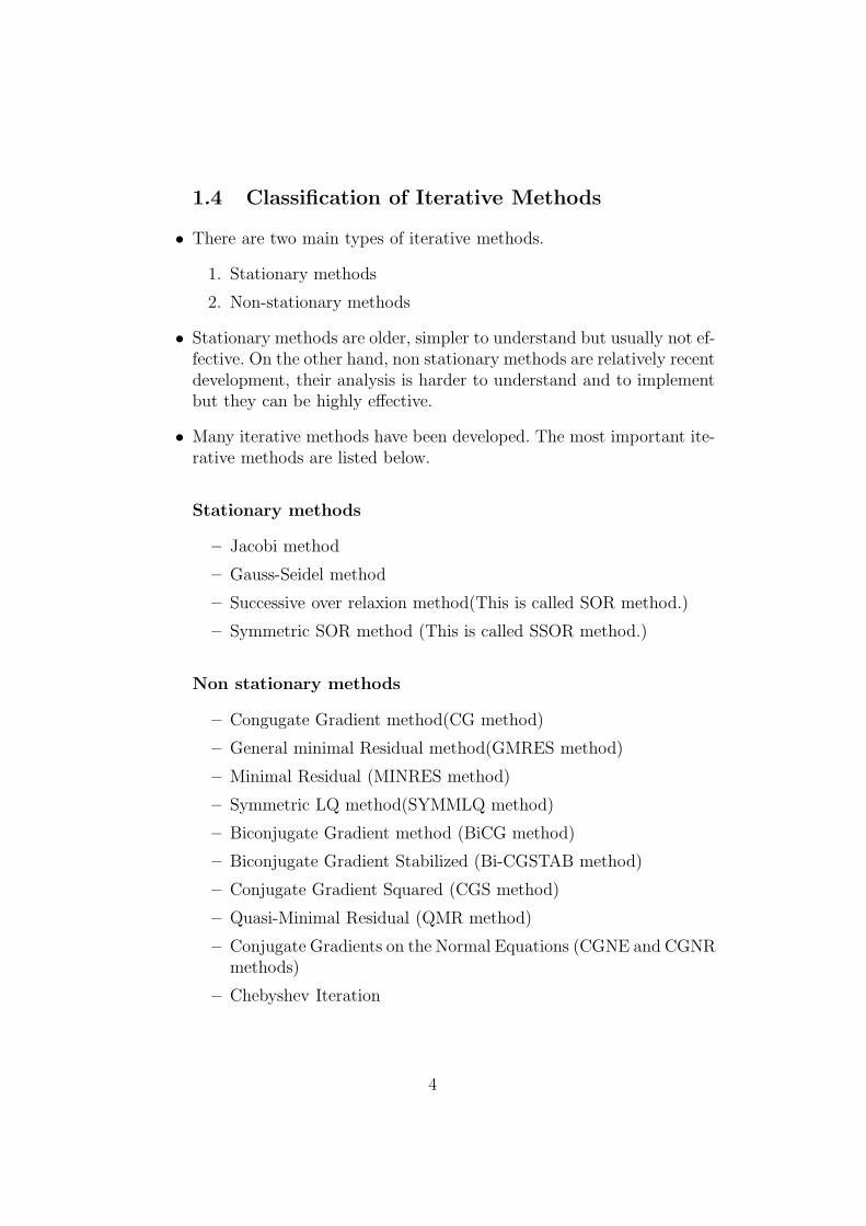
1.4 Classification of Iterative Methods

• There are two main types of iterative methods.

1. Stationary methods

2. Non-stationary methods

• Stationary methods are older, simpler to understand but usually not ef-fective. On the other hand, non stationary methods are relatively recentdevelopment, their analysis is harder to understand and to implementbut they can be highly effective.

• Many iterative methods have been developed. The most important ite-rative methods are listed below.

Stationary methods

– Jacobi method

– Gauss-Seidel method

– Successive over relaxion method(This is called SOR method.)

– Symmetric SOR method (This is called SSOR method.)

Non stationary methods

– Congugate Gradient method(CG method)

– General minimal Residual method(GMRES method)

– Minimal Residual (MINRES method)

– Symmetric LQ method(SYMMLQ method)

– Biconjugate Gradient method (BiCG method)

– Biconjugate Gradient Stabilized (Bi-CGSTAB method)

– Conjugate Gradient Squared (CGS method)

– Quasi-Minimal Residual (QMR method)

– Conjugate Gradients on the Normal Equations (CGNE and CGNRmethods)

– Chebyshev Iteration

4

• Remark:All of the above listed non-stationary methods except Chebyshev Ite-ration are Krylov Subspace methods.

�

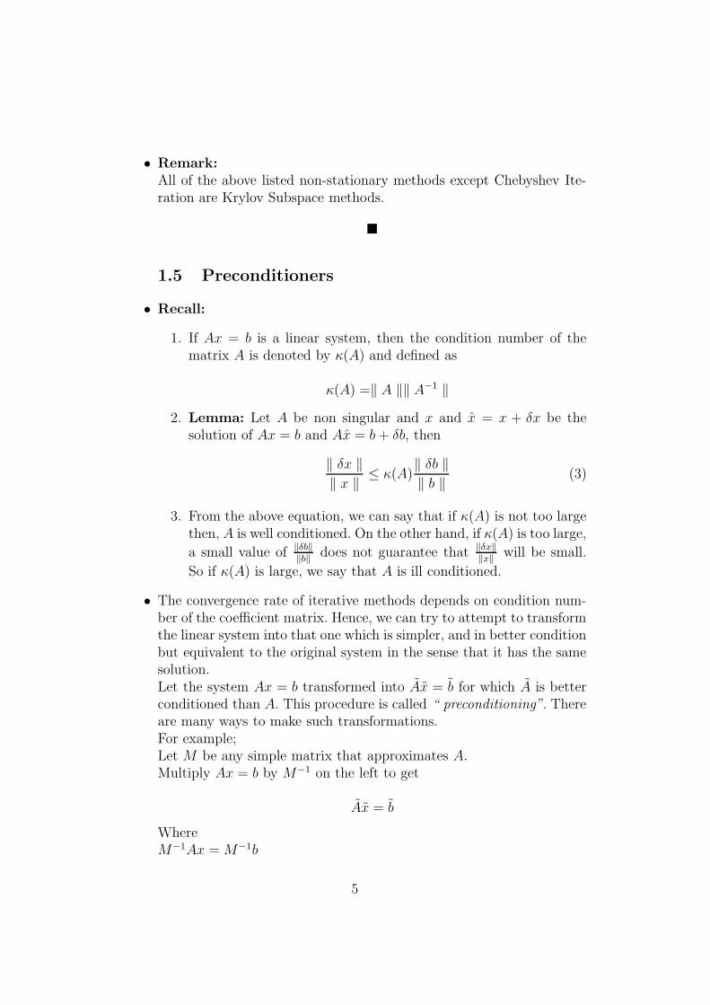
1.5 Preconditioners

• Recall:

1. If Ax = b is a linear system, then the condition number of thematrix A is denoted by κ(A) and defined as

κ(A) =‖ A ‖‖ A−1 ‖

2. Lemma: Let A be non singular and x and x = x + δx be thesolution of Ax = b and Ax = b + δb, then

‖ δx ‖

‖ x ‖≤ κ(A)

‖ δb ‖

‖ b ‖(3)

3. From the above equation, we can say that if κ(A) is not too largethen, A is well conditioned. On the other hand, if κ(A) is too large,

a small value of ‖δb‖‖b‖

does not guarantee that ‖δx‖‖x‖

will be small.

So if κ(A) is large, we say that A is ill conditioned.

• The convergence rate of iterative methods depends on condition num-ber of the coefficient matrix. Hence, we can try to attempt to transformthe linear system into that one which is simpler, and in better conditionbut equivalent to the original system in the sense that it has the samesolution.Let the system Ax = b transformed into Ax = b for which A is betterconditioned than A. This procedure is called “ preconditioning”. Thereare many ways to make such transformations.For example;Let M be any simple matrix that approximates A.Multiply Ax = b by M−1 on the left to get

Ax = b

WhereM−1Ax = M−1b

5

A = M−1A

b = M−1b

x = x

�

2 Historical Background

• Since the early 1800s, researchers have been attracted towards iterationmethods to approximate the solutions of large linear systems.

• The first iterative method for system of linear equations is due to KarlFriedrich Gauss. His least square method led him to a system of equati-ons which is called “ Block wise Gauss-seidel method”. The others whoplayed an important role in the development of iterative methods, are:

– Carl Gustav Jacobi

– David Young

– Richard Varga

– Cornelius Lanczos

– Walter Arnoldi

– and so on

• From the beginning, scientists and researchers used to have both po-sitive and negative feelings about the iterative methods because theyare better in comparison of direct methods but the so-called statio-nary iterative methods like Jacobi, Gauss Seidel and SOR methods ingeneral converge too slow to the solution of practical use. In the mid1950’s, the observation in Ewald Bodewig’s textbook was that iterationmethods were not useful, except when A approaches a diagonal matrix.

• Despite the negative feelings, researchers continued to design the fasteriterative methods.

• Around the early 1950’s the idea of Krylov subspace iteration was esta-blished by Cornelius Lanczos and Walter Arnoldi. Lanczos’ method was

6

based on two mutually orthogonal vector sequences and his motivationcame from eigenvalue problems. In that context, the most prominentfeature of the method is that it reduces the original matrix to tridiago-nal form. Lanczos later applied his method to solve linear systems, inparticular the symmetric ones.

• In 1952, Magnus Hestenes and Eduard Stiefel presented a paper [1]which is about the classical description of the conjugate gradient me-thod for solving linear systems. Although error-reduction properties areproved and experiments showing premature convergence are reportedin this paper, the conjugate gradient method is presented here as adirect method, rather than an iterative method.

• This Hestenes/Stiefel method is closely related to a reduction of theLanczos method to symmetric matrices, reducing the two mutuallyorthogonal sequences to one orthogonal sequence, but there is an im-portant algorithmic difference. Whereas Lanczos used three-term re-currences, the method by Hestenes and Stiefel uses coupled two-termrecurrences. By combining the two two-term recurrences (eliminatingthe “search directions”) the Lanczos method is obtained.

• The Conjugate gradient method did not receive much recognition in itsfirst 20 years because of the lack of exactness. Later researchers realizedthat this method is more fruitful to consider as truly iterative method.John Reid (in 1972) was the first one who pointed out in this direction.Moreover, it is now an important and cheaper iterative method for thesymmetric case.

• Similarly, for the nonsymmetric case, GMRES method was proposedin 1986 by Youcef Saad and Martin Schultz. This method is based onArnoldi algorithm and it is comparatively expensive. In this method,one has to store a full orthogonal basis for the Krylov subspace fornonsymmetric matrix A, which means the more iterations, the morebasis vectors one must store. For many practical problems, GMREScan take hundreds of iterations, which makes a full GMRES unfeasable.This led to a search for cheaper near-optimal methods.

• Vance Faber and Thomas Manteuffel’s famous result showed that ge-nerally there is no possibility of constructing optimal solutions in theKrylov subspace for nonsymmetric matrix A by short recurrences, asin the conjugate gradients method,

7

• The generalization of conjugate gradients for nonsymmetric systems,i.e. Bi-CG, often displays an irregular convergence behavior, includinga possible breakdown. Roland Freund and Noel Nachtigal gave an ele-gant remedy for both phenomena in their QMR method. BiCG andQMR have the disadvantage that they require an operation with AT

per iteration step. This additional operation does not lead to a furtherresidual reduction.

• In the mid 1980s, Peter Sonneveld recognized that one can use the AT

operation for a further residual reduction through a minor modifica-tion to the Bi-CG scheme, almost without additional computationalcosts which is called CGS method. This method was often faster butsignificantly more irregular.

• In 1992, Henk A. van der Vorst, showed that Bi-CG could be made fa-ster and smoother, at almost no additional cost, with minimal residualsteps.i.e. Bi-CGSTAB algorithm.

• Another class of acceleration methods that has been developed sincearound 1980, are the multigrid or multilevel methods. These methodsapply to grid-oriented problems, and the idea is to work with coarseand fine grids.

�

2.1 Current Research Areas

• Although, multigrid methods are faster and efficient, there is no clearseparation between the multigrid methods and Krylov methods becauseone can use the multigrid as a preconditioner for Krylov methods forless regular problems and the Krylov techniques are as smoothers formultigrid. So this is one of the fruitful direction for further exploration.

• In the past Researchers have been trying to find a new and betterKrylov methods which converge in a less number of iterations. Theconvergence of a Krylov method depends on whether you are able todefine a nearby matrix K that will serve as a preconditioner or not.Recent research is more oriented in that direction(i.e. to find a betterpreconditioner) than in trying to improve the Krylov subspace methods.

�

8

3 Krylov Subspace Iteration

• Krylov Subspace Iterations or Krylov Subspace Methods (or one can sayonly Krylov Methods) are a subset of non-stationary iterative methods.They are used as

1. linear system solvers

2. iterative solvers of eigenvalue problems.

• Recall:

1. Definition: For the given two vectors x = [x1, x2, x3, ......, xn]T

and y = [y1, y2, y3, ......, yn] in Rn, the inner product of the twovectors x and y is denoted by 〈x, y〉 and defined as

〈x, y〉 =n∑

i=1

xiyi

2. Although the inner product is a real number, it can be expressedas a matrix product.

〈x, y〉 = xT y = yTx

3. Definition: Any matrix A is symmetric if

A = AT

and positive definite if

xT Ax > 0 for all x 6= 0

4. Any matrix is called symmetric positive definite (SPD) if it issymmetric and positive definite.

• Most important Krylov methods for solving linear system and for sol-ving eigenvalue problems are listed below.

9

Type of Matrix Krylov methods for Ax = b Krylov methods for Ax = λx

A = SPD CG LanczosCGNECGNR

GMRES Bi-LanczosBiCG ArnoldiBi-CGSTABMINRES

A 6= SPD SYMMLQCGSQMR

• Here we will concentrate on those methods which are used as linearsystem solvers but first let us define a Krylov subspace and recall someof its elementary properties.

�

3.1 Definition and Elementary properties

• Definition: Let A ∈ Rn×n and v ∈ Rn with v 6= 0 then,

– The sequence of the form

v, Av, A2v, A3v, ...,

is called Krylov sequence.

– The Matrix of the form

Kk(A, v) = [v, Av, A2v, A3v, ..., Ak−1v]

is called the kth Krylov Matrix associated with A and v.

– The corresponding subspace

Kκ(A, v) = span{v, Av, A2v, A3v, ..., Ak−1v}

is called the kth Krylov subspace or Krylov Space associated withA and v.

10

• Lemma Let A ∈ Rn×n and v ∈ Rn with v 6= 0 then,

1. Kκ(A, v) ⊆ Kκ+1(A, v) and AKκ(A, v) ⊆ Kκ+1(A, v)

2. If σ 6= 0, Kκ(A, v) = Kκ(σA, v) = Kκ(A, σv)

i.e. Krylov Space remains unchanged when either A or v is scaled.

3. For any c Kκ(A, v) = K(A − cI, v)

i.e. Krylov Space is invariant under Shifting.

4. Kκ(W−1AW, W−1v) = W−1Kκ(A, v)

i.e. Krylov Space behaves in a predictable way under similaritytransformation.

�

• Theorem The space Kκ(A, v) can be written in the form

Kκ(A, v) = {p(A)(v) : p is a polynomial of degree at most k − 1}

�

• Theorem The Krylov sequence v, Av, A2v, A3v, ... terminates at l if l

is the smallest integer s.t.

Kl+i(A, v) = Kl(A, v)

anddim[Kl+i(A, v)] = dim[Kl(A, v)]

�

3.2 Basic Idea of Krylov solvers

• In Krylov subspace methods, we keep all computed approximants {xi}and combine them for a better solution. Define the Krylov Subspace as

Kn(A, r0) = span{r0, Ar0, A2r0, a

3r0, ......, An−1r0}

wherer0 = b − Ax0.

11

• If the vectors r0, Ar0, ..., An−1r0, spanning the Krylov subspace Kn(A, r0),

are linearly independent, we note that

dimKn(A, r0) = n

As soon as Anr0 ∈ Kn(A, r0), we obtain that

Kn+i(A, r0) = Kn(A, r0) for all i ∈ N .

and we get a linear combination

0 = c0r0 + c1Ar0 + ... + cn−1An−1r0 + cnAnr0

where at least cn 6= 0 and c0 6= 0, otherwise the multiplication by A−1

would contradict the assumption that the vectors r0, Ar0, ..., An−1r0 are

linearly independent.Indeed as c0 6= 0 we get;

A−1r0 =−1

c0

n∑

i=1

ciAi−1r0 ∈ Kn(A, r0) (4)

The smallest index n with

n = dim[Kn(A, r0)] = dim[Kn+1(A, r0)

is called the grade of A with respect to r0 and denoted by r(A, r0).

�

• Remarks:

1. The above argument also shows that there is no smaller Krylovsubspace which contains A−1r0; therefore

r(A, r0) = min{n : A−1r0 ∈ Kn(A, r0)}

2. The degree of the minimum polynomial of A is an upper boundfor r(A, r0).

• The basic idea of a Krylov solver is to construct a sequence of appro-ximations getting closer to the exact solution x∗, such that

xn ∈ x0 + Kn(A, r0) (5)

12

where x0 is the initial approximation,

ri = b − Axi (6)

is the ith residual andei = xi − x∗ (7)

denotes the ith error. After r(A, r0) iterations the exact solution is con-tained in the current affine Krylov subspace, i.e.

x∗ ∈ x0 + Kr(A, r0) (8)

as x0 + A−1r0 = x0 + A−1(Ax∗ − Ax0) = x∗

�

3.3 Conjugate Gradient Method

• Conjugate gradient method is kind of Krylov Subspace method. As weexplained in above table, this method is especially for symmetric andpositive definite matrix A. The problem of solving Ax = b by conjugategradient method can also be known as a minimization problem.

3.3.1 Quadratic Form

• Definition: Define a function J : Rn → R by

J(x) =1

2xT Ax − xT b + c (9)

Where A is a matrix x and b are vectors and c is a scalar constant.Then the function J(x) is said to be quadratic form.

• In addition, the gradient of a quadratic form F (x) is defined as

5F = F ′(x) = [∂

∂x1F,

∂

∂x2F, ........

∂

∂xn

F ]T

=⇒ 5F = F ′(x) =

∂∂x1

F∂

∂x2F

.

.

.∂

∂xnF

(10)

13

Using calculus from equations (9) and (10), one can get

5F =1

2AT x +

1

2AT x − b (11)

If A is Symmetric, this equation can be reduced to

5F = Ax − b (12)

• Here is a very simple example of linear system to show the geometricmeaning of quadratic form and its gradient which will help us to un-derstand conjugate method well and easily.The system of linear quations3x1 + 2x2 = 22x1 + 6x2 = −8is given by Ax = b where

A =

[3 22 6

]

, x =

[x1

x2

]

and b =

[2−8

]

• The system Ax = b is illustrated in fig.1. In general x∗ lies at theintersection point of n hyperplanes each having dimension n − 1. Forthe above mentioned problem, the solution is

x∗ =[

2 −2]T

14

Abbildung 1: Sample of two dimensio-nal linear system

15

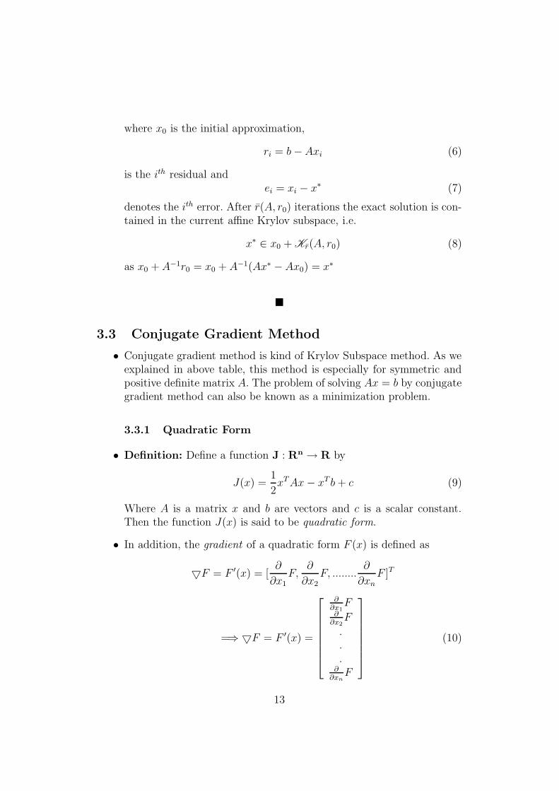
• The visualization of the quadratic form of above system of linear equa-tion where the constant c of the quadratic form is zero, is in the fig.2.

Abbildung 2: Graph of a quadraticform F (x). The minimum point of thissurface is the solution to Ax = b.

16

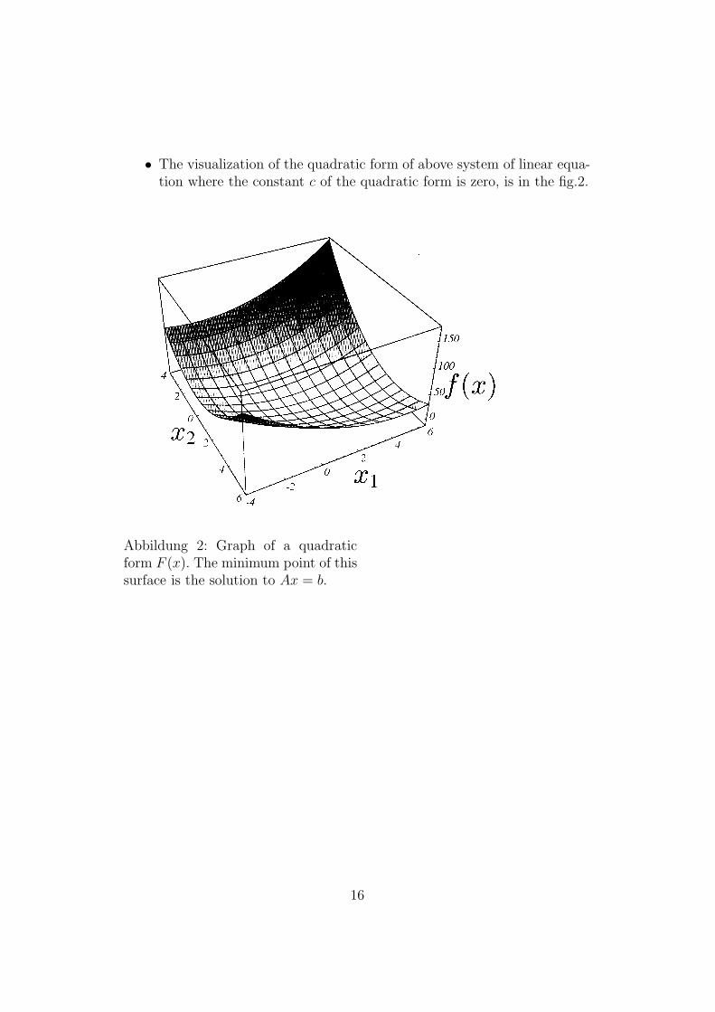
Abbildung 3: Contours of the quadratic form.

17

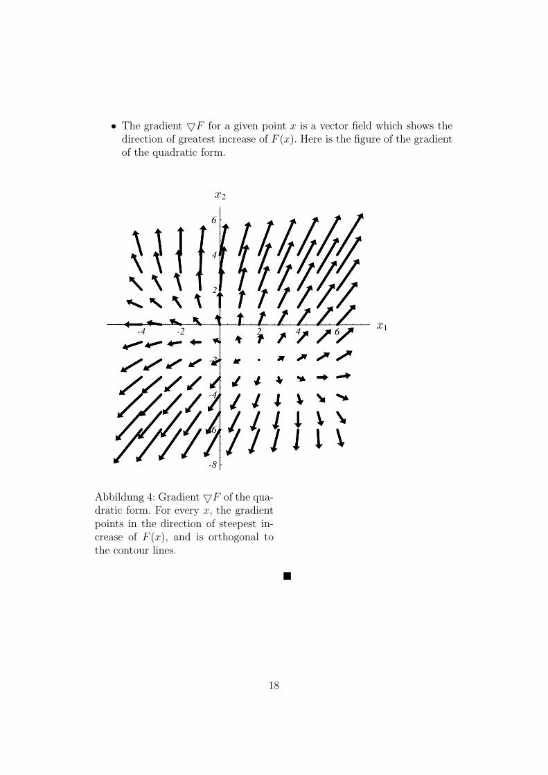
• The gradient 5F for a given point x is a vector field which shows thedirection of greatest increase of F (x). Here is the figure of the gradientof the quadratic form.

Abbildung 4: Gradient 5F of the qua-dratic form. For every x, the gradientpoints in the direction of steepest in-crease of F (x), and is orthogonal tothe contour lines.

�

18

3.3.2 Minimization of Quadratic Form

• The gradient of F (x) at the bottom of the paraboloid bowl( fig (2)) iszero. So one can minimize F (x) by setting

5F = F ′(x) = 0

Setting 5F = 0, on equation (11) we get

Ax − b = 0 ⇒ Ax = b

which is our linear system to be solved. Thus, if A is positive definiteand symmetric, then the solution of Ax = b is the minimization ofF (x).

• Claim: Let A ∈ Rn×n be positive definite, b ∈ Rn and a function F isdefined as in (3), then there exists exactly one x∗ ∈ Rn for whichF (x∗) = min{F (x)}and this x∗ is the solution of Ax = b also.

Proof:The function is quadratic in x1, x2, x3, .....xn,. Let x∗ denote the solu-tion of Ax = b. ThenF (x) = 1

2xT Ax − xT Ax∗

= 12xT Ax − xT Ax∗ + 1

2x∗T Ax∗ − 1

2x∗T Ax∗

=1

2(x − x∗)T A(x − x∗)

︸ ︷︷ ︸

on which F (x) depends.

−1

2x∗T Ax∗

︸ ︷︷ ︸

independent of x

So we can say that F (x) is minimized only when 12(x − x∗)T A(x − x∗)

is minimized.In this expression, A is positive definite. So we can say that the term12x∗T Ax∗ is positive unless x − x∗ = 0.

=⇒ F (x) is minimum if and only if y = x.

�

• To minimize F (x), we take a series of steps in the direction in whichF (x) decreases most quickly.i.e. which is the direction opposite to 5F .

19

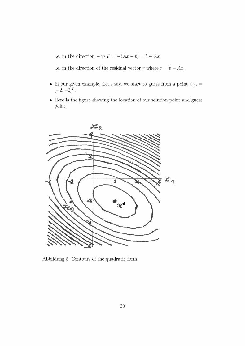
i.e. in the direction −5 F = −(Ax − b) = b − Ax

i.e. in the direction of the residual vector r where r = b − Ax.

• In our given example, Let’s say, we start to guess from a point x(0) =[−2,−2]T .

• Here is the figure showing the location of our solution point and guesspoint.

Abbildung 5: Contours of the quadratic form.

20

• Remarks

1. The error ei = x(i) − x is a vector that indicates how far we arefrom the solution.

2. The residual r(i)=b−Ax(i)indicates how far we are from the correct

value of b.

3. The relation between r(i) and e(i) is given by r(i) = −Ae(i) = −5F .

�

3.3.3 Conjugate Gradient Algorithm

• Definition: Two vectors vi and vj are said to be A-orthogonal or con-jugate to each other with respect to symmetric positive matrix A if

vTi Avj = 0 for all i 6= j

⇒ (vi, vj) = 0∀i 6= j

• Let us consider a set of A−congugate search directions(vectors) {d(0), d(1), d(2), ....., d(n)}and the residual

r0 = Ax0 (13)

andd0 = r0 (14)

Now, we start from a search line

x(1) = x(0) + αd(0) (15)

21

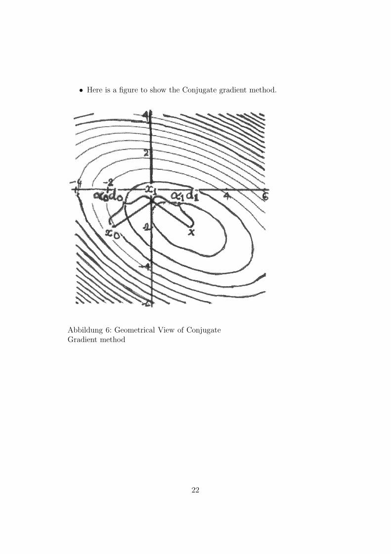
• Here is a figure to show the Conjugate gradient method.

Abbildung 6: Geometrical View of ConjugateGradient method

22

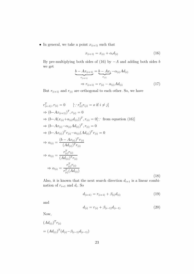
• In general, we take a point x(i+1) such that

x(i+1) = x(i) + αid(i) (16)

By pre-multiplying both sides of (16) by −A and adding both sides b

we getb − Ax(i+1)︸ ︷︷ ︸

r(i+1)

= b − Axi︸ ︷︷ ︸

r(i)

−α(i)Ad(i)

⇒ r(i+1) = r(i) − α(i)Ad(i) (17)

But r(i+1) and r(i) are orthogonal to each other. So, we have

rT(i+1), r(i) = 0 [∵ rT

(i)r(j) = o if i 6= j]

⇒ (b−Ax(i+1))T , r(i) = 0

⇒ (b−A(x(i)+α(i)d(i)))T , r(i) = 0[∵ from equation (16)]

⇒ (b−Ax(i)−α(i)Ad(i))T , r(i) = 0

⇒ (b−Ax(i))T r(i)−α(i)(Ad(i))

T r(i) = 0

⇒ α(i) =(b − Ax(i))

T r(i)

(Ad(i))T r(i)

⇒ α(i) =rT(i)r(i)

(Ad(i))T r(i)

⇒ α(i) =rT(i)r(i)

rT(i)(Ad(i))

(18)Also, it is known that the next search direction di+1 is a linear combi-nation of ri+1 and di. So

d(i+1) = r(i+1) + β(i)d(i) (19)

andd(i) = r(i) + β(i−1)d(i−1) (20)

Now,

(Ad(i))T r(i)

= (Ad(i))T (d(i)−β(i−1)d(i−1))

23

= (Ad(i))T d(i)−β(i−1)(Ad(i))

T d(i−1)︸ ︷︷ ︸

=0

= (Ad(i))T d(i)

∴ (Ad(i))T r(i) = (Ad(i))

T d(i) (21)

From the equation (18) and (21), we get

α(i) =(r(i))

T r(i)

(Ad(i))T , d(i)

(22)

In addition, d(i+1) is orthogonal to Ad(i). So, we get

(d(i+1))T (Ad(i)) = 0

⇒ (r(i+1)+β(i)d(i))T (Ad(i)) = 0 [∵ From equation (20) ]

⇒ (r(i+1))T (Ad(i))+β(i)(d(i))T (Ad(i)) = 0

⇒ (r(i+1))T (Ad(i)) = −β(i)(d(i))T (Ad(i))

⇒ β(i) =−(r(i+1))

T (Ad(i))

(d(i))T (Ad(i))

∴ β(i) =−(r(i+1))

T (Ad(i))

(d(i))T (Ad(i))(23)

Note That from recurrence equation (17),

Ad(i) =−1

α(i)

(r(i+1) − r(i)) (24)

So, from equation (23) and (24), we get

β(i) =1

α

(r(i+1))T (r(i+1) − r(i))

(d(i))T (Ad(i))

Put the value of α on this relation,

β(i) =1

(r(i))T (r(i))

(Ad(i))T ,d(i)

(r(i+1))T (r(i+1)) − (r(i+1))

T (r(i))

(d(i))T (Ad(i))

⇒ β(i) =(r(i+1))

T (r(i+1))

(r(i))T (r(i))(25)

Putting all these above relations together, we get the following Algo-rithm.

24

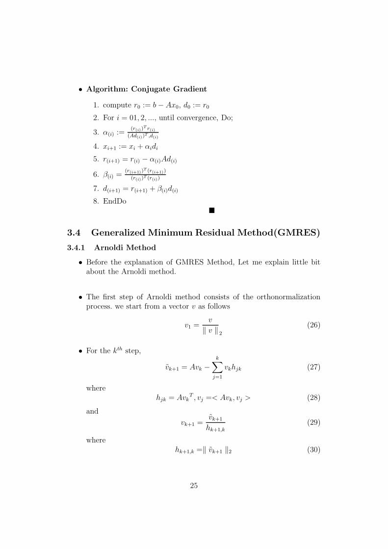
• Algorithm: Conjugate Gradient

1. compute r0 := b − Ax0, d0 := r0

2. For i = 01, 2, ..., until convergence, Do;

3. α(i) :=(r(i))

T r(i)

(Ad(i))T ,d(i)

4. xi+1 := xi + αidi

5. r(i+1) = r(i) − α(i)Ad(i)

6. β(i) =(r(i+1))

T (r(i+1))

(r(i))T (r(i))

7. d(i+1) = r(i+1) + β(i)d(i)

8. EndDo�

3.4 Generalized Minimum Residual Method(GMRES)

3.4.1 Arnoldi Method

• Before the explanation of GMRES Method, Let me explain little bitabout the Arnoldi method.

• The first step of Arnoldi method consists of the orthonormalizationprocess. we start from a vector v as follows

v1 =v

‖ v ‖2

(26)

• For the kth step,

vk+1 = Avk −k∑

j=1

vkhjk (27)

wherehjk = Avk

T , vj =< Avk, vj > (28)

and

vk+1 =vk+1

hk+1,k

(29)

wherehk+1,k =‖ vk+1 ‖2 (30)

25

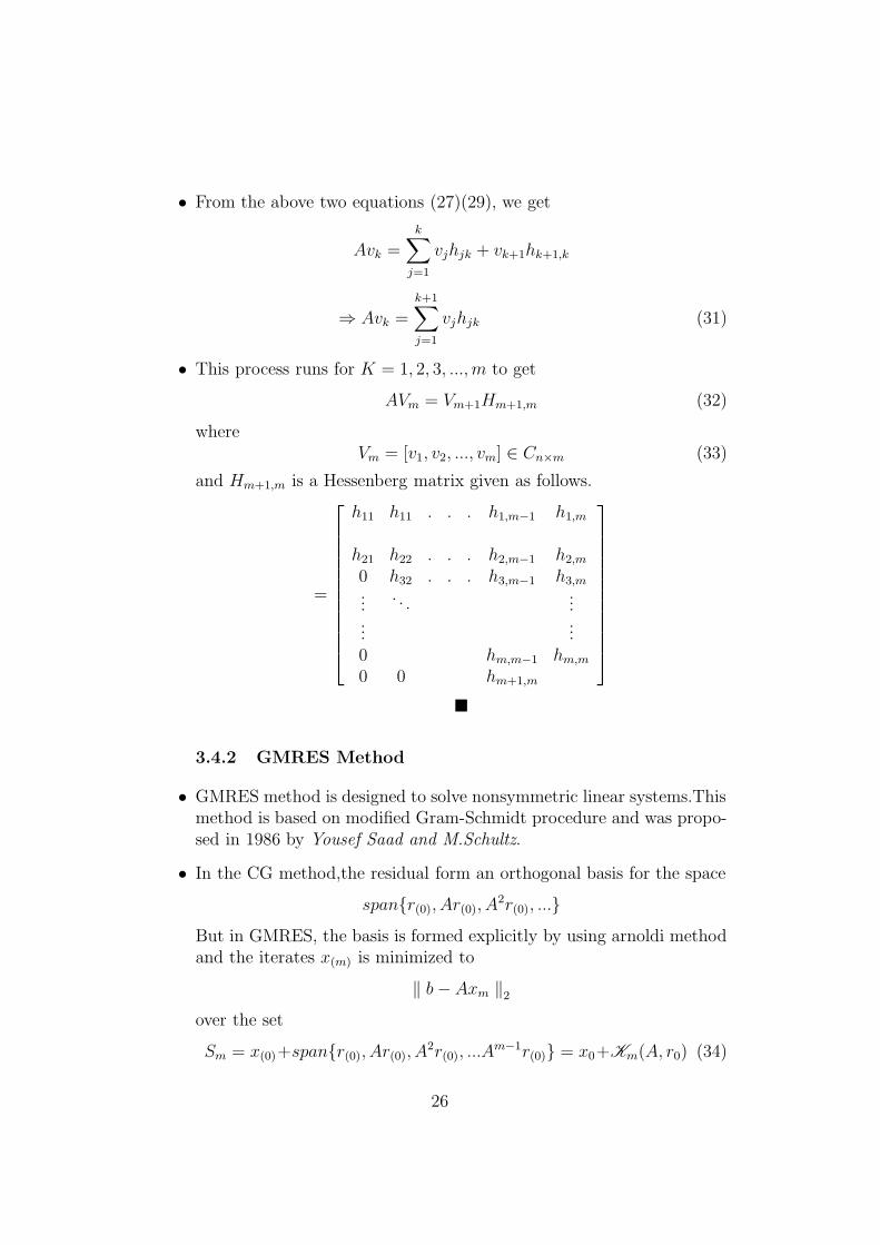
• From the above two equations (27)(29), we get

Avk =

k∑

j=1

vjhjk + vk+1hk+1,k

⇒ Avk =k+1∑

j=1

vjhjk (31)

• This process runs for K = 1, 2, 3, ..., m to get

AVm = Vm+1Hm+1,m (32)

whereVm = [v1, v2, ..., vm] ∈ Cn×m (33)

and Hm+1,m is a Hessenberg matrix given as follows.

=

h11 h11 . . . h1,m−1 h1,m

h21 h22 . . . h2,m−1 h2,m

0 h32 . . . h3,m−1 h3,m

.... . .

......

...0 hm,m−1 hm,m

0 0 hm+1,m

�

3.4.2 GMRES Method

• GMRES method is designed to solve nonsymmetric linear systems.Thismethod is based on modified Gram-Schmidt procedure and was propo-sed in 1986 by Yousef Saad and M.Schultz.

• In the CG method,the residual form an orthogonal basis for the space

span{r(0), Ar(0), A2r(0), ...}

But in GMRES, the basis is formed explicitly by using arnoldi methodand the iterates x(m) is minimized to

‖ b − Axm ‖2

over the set

Sm = x(0)+span{r(0), Ar(0), A2r(0), ...A

m−1r(0)} = x0+Km(A, r0) (34)

26

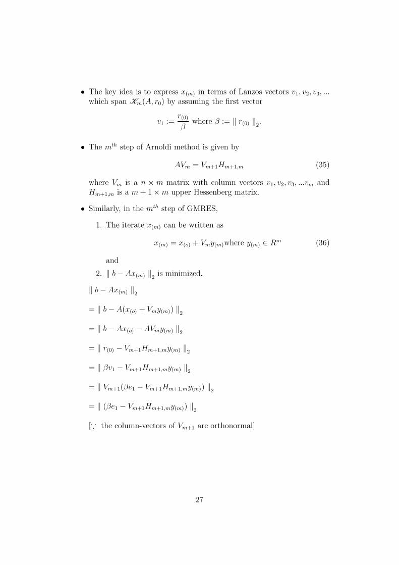
• The key idea is to express x(m) in terms of Lanzos vectors v1, v2, v3, ...

which span Km(A, r0) by assuming the first vector

v1 :=r(0)

βwhere β := ‖ r(0) ‖2

.

• The mth step of Arnoldi method is given by

AVm = Vm+1Hm+1,m (35)

where Vm is a n × m matrix with column vectors v1, v2, v3, ...vm andHm+1,m is a m + 1 × m upper Hessenberg matrix.

• Similarly, in the mth step of GMRES,

1. The iterate x(m) can be written as

x(m) = x(o) + Vmy(m)where y(m) ∈ Rm (36)

and

2. ‖ b − Ax(m) ‖2is minimized.

‖ b − Ax(m) ‖2

= ‖ b − A(x(o) + Vmy(m)) ‖2

= ‖ b − Ax(o) − AVmy(m) ‖2

= ‖ r(0) − Vm+1Hm+1,my(m) ‖2

= ‖ βv1 − Vm+1Hm+1,my(m) ‖2

= ‖ Vm+1(βe1 − Vm+1Hm+1,my(m)) ‖2

= ‖ (βe1 − Vm+1Hm+1,my(m)) ‖2

[∵ the column-vectors of Vm+1 are orthonormal]

27

• Algorithm: GMRES

1. compute r0 = b − Ax0, β = ‖ r0 ‖2 and V1 :=r(0)

β

2. Define the (m + 1) × m matrix Hm+1,m = {hij}1≤i≤m+1,1≤j≤m}.

Set Hm+1,m = 0.

3. For j = 01, 2, ..., m Do:

4. Compute wj := Avj

5. For i = 1, 2, ..., m Do;

6. hij := wTj vi

7. wj := wj − hijvi

8. EndDO

9. hj+1,j := ‖ wj ‖2.IF hj+1,j = 0,Set m := j and go to 12.

10. vj+1 =wj

hj+1,j

11. EndDO

12. Compute ‖ (βe1 − Vm+1Hm+1,my(m)) ‖2

which is the minimizer andxm = x0 + Vmym

28

• References

1. M. HESTENES AND E. STIEFEL, Methods of conjugate gradi-ents for solving linear systems, J. Res. Nat. Bur. Stand., 49 (1952),pp. 409-436.

2. W. ARNOLDI, The principle of minimized iterations in the so-lution of the matrix eigenvalue problem, Quart. Appl. Math., 9(1951), pp. 17-29

3. Jonathan Richard Shewchuk, An Introduction to the ConjugateGradient Method Without the Agonizing Pain,under the webhttp://www.cs.ucdavis.edu/ bai/ECS231/schewchukcgpaper.pdf

4. Yousef Saad, Iterative methods for Sparse Linearsystems

5. Henk A. van der Vorst, The article on “KRYLOV SUBSPACEITERATION” of the journal Computing in Science and Enginee-ring; 2000.

29