Shimer Meets the Production Based Asset Pricing Crowd:

Labor Search and Asset Returns�

Hyung Seok Eric Keam

Sogang University, South Korea

John B. Donaldson

Columbia University

April 5, 2011

Abstract

THIS IS THE LATEST ONE. Beginning with Shimer (2005) and Hall (2005), a recent branch

of the business cycle literature has explored the role of wage rigidity in accounting for the statistical

characteristics of key labor market variables over the business cycle; in particular, high vacancy and

unemployment volatility and a high negative correlation between the two. As a further exploration,

we extend the Mortensen-Pissarides structure of period-by-period Nash wage bargaining to an en-

vironment where there is labor force heterogeneity (permanently employed "insiders" and outsiders

subject to separations) and limited participation in the �nancial asset markets. We show that a

reasonable calibration of the resulting model satisfactorily accounts not only for aggregate �uctua-

tions in unemployment and vacancies and their cross-correlations but also for the observed wedge

between variations at the intensive margin (hours per worker) and at the extensive margin (total

hours). The model also achieves a satisfactory replication of the major �nancial return phenomena;

namely, a low risk-free rate, a high equity premium, and an upward sloping term structure. The

key to these results is the variable income insurance e¤ectively provided by shareholders and given

to workers arising from the interaction of Nash wage bargaining superimposed on the incomplete

�nancial market structure. We refer to the variable income insurance as (income) distribution risk.

Keywords: Nash bargaining; business cycles; equity premium puzzle; limitedparticipation

�This paper has bene�ted from discussions with Marc Giannoni, Bruce Preston, Paolo Siconol�, Stephanie Schmitt-Grohe, and Martin Uribe. The usual disclaimer applies.

1

1 Introduction

A recent body of research (e.g., Hall (2005) and Shimer (2005)) argues that the conventional search

model of employment dynamics due to Mortensen (1992) and Pissarides (1988, 1990) (MP hereafter)

cannot account for key cyclical movements in labor market variables when superimposed on standard real

business cycle paradigms. In particular, the high cyclical volatility of vacancies and unemployment as

well as their negative correlation at business cycle frequencies are statistical realities that are di¢ cult to

replicate in DSGE models. The consensus perspective on this anomaly has been that the MP mechanism

for wage determination accommodates too much wage �exibility. This excessive wage �exibility in turn

dampens the cyclical movements in �rms� incentives to hire and keeps vacancy and unemployment

volatilities counterfactually low.

In this paper we revisit these issues by adopting an expanded labor market modeling perspective:

while we retain the basic structure of labor market search cum period-by-period Nash wage bargaining,

we extent the MP model to a fully dynamic environment where the asset markets are incomplete and

perfect risk-sharing between capital owners and workers is not guaranteed. More speci�cally we develop

Nash wage bargaining between capitalists and workers within a macro model with limited stock market

participation, and emphasize the interactions of the labor and �nancial markets in a manner unique to

the DSGE literature. As a consequence, we are able to extend the ability of a basic DSGE construct

to explain not only the stylized facts of the business cycle and labor markets (especially those aspects

emphasized by Shimer (2005) and Hall (2005), but also the basic stylized �nancial facts as well.

The standard real business cycle model with a single persistent productivity shock and capital

adjustment costs is the foundation on which we build. As noted, there are two types of agents: insider-

stockholders and outsider-worker-non-stockholders. The former have full access to �nancial markets,

namely the stock and bond markets. In contrast, the latter group, who comprise the majority of

households, do not participate in the stock market but trade only in the risk free bond market. Default

free bonds are thus available to all households. The assumption of limited asset market participation

is empirically appropriate: it is well documented that more than two thirds of US households held no

stock prior to the 1990s, and that households in the top 20% of the wealth distribution alone owned

more than 98% of stocks during the 1990s, despite the stock market participation rate having increased

substantially during this period (Mankiw and Zeldes (1991) and Poterba (2000)).

What emerges in this setting is a Nash wage bargaining outcome between capital owners and workers

in which vacancy postings and unemployment levels are substantially in�uenced by the pattern of capital

market participation. Both mechanisms by which �rm owners and workers interact reinforce one another

to reduce wage volatility. In particular, ceteris paribus, restricted capital market participation has the

equilibrium consequence of shareholders providing workers with partial insurance against their labor

income variation (see also Danthine and Donaldson (2002) and Guvenen (2003, 2009)). This insurance

2

is manifest as countercyclical variation in the income shares of workers in the presence of low wage

volatility. More speci�cally, a high productivity realization coincides with the situations where wage

bills rise less than output in the short run. Conversely, a lower productivity realization coincides with

situations where the wage bill falls less than output in the short run. Since, ceteris paribus, Nash

bargaining wage outcomes also lead to a counter-cyclical wage income share, these e¤ects reinforce one

another to produce a very sluggish response of wages to productivity shocks. This sluggish response

of wage income to output variation over the business cycle we entitle the �operating leverage e¤ect�

because, like �nancial leverage, it has the consequence of increasing the income risk to shareholders

with implications for the equity premium and other �nancial quantities.

At the same time, stockholders are hindered from smoothing their consumption in two ways: �rst,

capital adjustment costs discourage consumption smoothing via investment variation and, second, the

frictional cost of wage variation due to the income insurance mechanism discourages adjustments along

the wage dimension as well. As a result, shareholders attempt to smooth their own consumption

by adjusting employment at the extensive margin: high productivity shock realizations dramatically

increase job vacancies and employment, while low productivity shocks substantially decrease them.

This set of events resolves the unemployment and vacancy volatility puzzles raised by Shimer (2005), as

well as reproducing their negative correlation. In fact, the model formulation presented here gives rise to

much greater vacancy and unemployment volatility than is found in the seminal models of Andol�atto

(1996), Merz (1995), and Gertler and Trigari (2009), which e¤ectively assume a complete asset market

structure.

Shareholder income variation arising from the partial insurance they provide to workers due to

the incomplete asset market structure signi�cantly a¤ects the Nash wage bargaining position of the

�rm acting on their behalf. Accordingly, we view this income distribution risk as akin to Shimer�s

(2005) hypothesized ad hoc Nash bargaining power shock, and, as such, our model can also be viewed as

suggesting micro-foundations for that device. More speci�cally, we may interpret our model as indirectly

providing an answer to the question posed by Shimer:�It seems plausible that a model with a combination

of wage and labor productivity shocks could generate the observed behavior of unemployment, vacancies

and real wages. . . the unanswered question is what exactly a wage shock is�(Shimer (2005, p. 42)). In

our framework that shock represents wage income variation arising from market incompleteness, and

the (partial) income insurance provided to workers by stockholders.

In summary, the principal contribution of this paper is to propose a reasonable and tractable mech-

anism that resolves the unemployment and vacancy volatility puzzles emphasized by Shimer (2005) and

Hall (2005), while, at the same time, enabling the model to achieve a satisfactory resolution of long-

standing major �nancial asset pricing puzzles. More speci�cally, we postulate Nash wage bargaining in

an environment where there is limited participation in the �nancial asset markets. What emerges from

these considerations is a fully endogenous Nash bargaining power shock, which we will identify with

3

(income) distribution risk, and which plays the key role in generating the operating leverage e¤ect in

our context. We then demonstrate that a reasonable calibration of the resulting model accounts not

only for aggregate �uctuation in unemployment and vacancies but also for the observed wedge between

variations at the intensive margin (hours per worker) and at the extensive margin (total hours) over

the business cycle. The model is also highly general in that its replication of the full range of labor

market statistics does not compromise its performance on the �nancial front, or with respect to the

major macroeconomic aggregates.

The structure of the paper is as follows. Section two presents the model and the de�nition of

equilibrium. Section 3 presents the basic results along the aggregates, labor market and �nancial

dimensions. Section 4 decomposes the model by attributing the overall pattern of results to those

individual model features principally responsible for them. It assesses, for example, the e¤ects of various

alternative preference speci�cations on the full range of results. Section 5 compares our results with

those arising from existing prominent models in the allied literature. Section 6 concludes.

2 The Model

We consider a discrete-time in�nite horizon economy with two distinct in�nitely lived agent types,

"insider-stockholders" and "outsider-nonstockholders." The continuum of "insider-stockholders" is dis-

tributed on a set of Lebesgue measure �s while the continuum of "outsider-nonstockholders" is indexed

on a set of Lebesgue measure 1.

2.1 Insider-stockholder

Following Guvenen (2003) the insider-stockholder, endowed with one unit of time, supplies labor services

to the (representative) �rm and trades securities�both equity claims to the �rm�s net income stream, and

a one-period risk-free real bond. What distinguishes our model from the Guvenen (2003) model, however,

is that the insider-stockholder trades his labor services exclusively in the segmented labor market for

insider-stockholders. This market is characterized by employment adjusting along the intensive margin

only; i.e., the labor income risk of the insider-stockholder entirely originates from �uctuations in hours

worked, not in total employment. This environment implies that the �rm and insider-stockholders have

a permanent relationship. As Barro (1997) points out, wages are thus not allocational. The environment

also can be viewed as nesting in a Lucas (1978b) span of control setup or a Rosen (1982) hierarchy,

where workers are assigned to managerial, production, and non-market tasks based on their comparative

advantage.

Given his information set st , the representative insider-stockholder smaximizes his lifetime expected

utility as given by:

4

V s(s0) = maxfhst ;cst ;est+1;bst+1g

E0

1Xt=0

�t[u(cst �Xt; hst )] (1)

s.t.

cst + petest+1 + p

ft bst+1 � wsth

st + (p

et + dt)e

st + p

ft bst (2)

where u denotes his period utility function, cst his period t consumption, and hst his period t labor hours.

The variable Xt represents the exogenous habit stock; it evolves according to

Xt = �Xt�1 + (1� �)��cst�1

where � is the habit parameter of the insider-stockholder group, and �cst�1 is the average consumption

level of the entire insider-stockholder group in the previous period:

�cst�1 �1

�s

Zcst�1d{

with { standing for the measure of insider-stockholders. In addition, dt denotes the aggregate period

t dividend payment by the �rm to its stockholders and est and bst , respectively, his period t stock and

bond holdings. The corresponding period t prices of these securities are pet and pft . Lastly, wst is

the insider-stockholder�s wage rate, exogenous from his perspective while Est � E( � j st ) denotes hisexpectations operator conditional on his information set st . The parameter � is the economy-wide

subjective discount factor.

We adopt a variation of GHH preference for the insider-stockholder:

u(cst �Xt; hst ) = u(cst �Xt �H(hst ))

where H(�) is his disutility of labor hours. This speci�cation of the period utility function combinesthe standard GHH preference with a special form of external habit formation or "catching up with the

Joneses" (see Abel (1990)). By neglecting the lagged average consumption level of the whole insider-

stockholder group (� = 0), the preference function speci�ed above is reduced to the standard GHH

utility function widely employed in the investment-shock literature (Greenwood, Hercowitz, and Hu¤man

(1988)). It is well known that the GHH class of preferences has an extremely weak short-run wealth

e¤ect on the labor supply. More speci�cally, the Hicksian wealth e¤ect of a real wage increase on hours

worked is zero for this class of preferences.1 Knowledge of this fact helps to de�ne the representative

insider-stockholder correctly; otherwise, the representative insider-stockholder will decrease his labor

1For more detail, see Jaimovich and Rebelo (2009).

5

supply in response to a positive productivity shock because of the short-run wealth e¤ect.

Moreover, the GHH class of preferences features a marginal rate of substitution between consump-

tion and labor supply that depends only on the labor supply itself. That is, the labor supply is deter-

mined independently of intertemporal consumption-savings choice and thus the e¤ect of intertemporal

consumption substitution on the labor supply is completely eliminated. Indeed, the marginal rate of

substitution between consumption and labor supply in this model economy reads as:

�uh(cst �Xt; h

st )

uc(cst �Xt; hst )= H1(h

st ): (3)

Conditional upon his information set st , the recursive formulation of the insider-stockholder�s prob-

lem is represented as:

V s(st ) = maxfcst ;hst ;est+1;bst+1g

2664u(cst �Xt; h

st )

+�st [wsthst + (p

et + dt)e

st + p

ft bst � cst � petest+1 � p

ft bst+1]

+�E(V s(st+1) j st )

3775 (4)

where �st is the Lagrange multiplier associated with the insider-stockholder�s budget constraint (2).

The solution to the above recursive problem (4) is characterized by the customary necessary and

su¢ cient �rst order conditions

wst = H1(hst ) (5)

pet = �Et[�st;t+1(p

et+1 + dt+1)] (6)

pft = �E(�st;t+1 j st )] (7)

where �st;t+1 denotes the insider-stockholder�s intertemporal marginal rate of substitution (IMRS).

2.2 Outsider-nonstockholder

We also postulate a continuum of in�nitely-lived outsider-nonstockholders, uniformly distributed on a set

of Lebesgue measure 1, who supply labor services via a Nash bargaining wage contract in their segmented

labor market (to be speci�ed). These agents di¤er from insider-stockholders in their investment opportu-

nity sets, job opportunity sets and consumption-smoothing motives. First, the outsider-nonstockholder

group is restricted from participating in the equity market, although they can freely trade one-period

risk-free bonds. This limited participation creates an asymmetry in consumption-smoothing opportuni-

ties; outsider-nonstockholders have to rely exclusively on the bond market, whereas insider-stockholders

have the additional tool of (indirectly) adjusting their physical capital holdings in response to productiv-

6

ity shocks. Second, we adopt heterogeneity in the preference speci�cation (Hornstein and Uhlig (1999))

for the baseline model: while capital owners (insider-stockholders) are subject to the "habit formation"

feature noted earlier, outsider-nonstockholder "at-will" workers are not. As Hornstein and Uhlig (2000)

suggests, this can be viewed as modelling the result of self-selection: agents who easily become accus-

tomed to a high consumption level, i.e. have habit formation preferences, may, over time, be more likely

to build up a large capital stock (physical and human) than agents who do not. It is therefore natural

to identify this group more closely with �rm ownership. In Section 4, we show, however, that the habit

formation feature of capitalists has a negligible e¤ect on the relatively volatile behavior of labor market

activity over the business cycles. In other words, the operating leverage e¤ect, which we emphasized

in the introduction and upon which our results crucially depend, is independent of the habit formation

of capitalists. Habit formation will still play an important role, however, in replicating the stylized

�nancial statistics.2

The third distinction is that outsider-nonstockholders trade their labor services exclusively in a

segmented labor market for outsider-nonstockholders with its own special characteristics. Unlike the

insider�s labor market, the outsider�s labor market is characterized by the variation in employment at the

extensive as well as the intensive margins. Another feature of this labor market arrangement is that �rms

and outsider-nonstockholders Nash bargain over wages in a context of search and matching frictions.

Since the model allows for heterogeneous agents, this wage bargaining is endogenously modi�ed to re�ect

the environment where the workers (outsider-nonstockholder) bargain over wages with the capital owners

(insider-stockholders). The resulting Nash bargaining wage is a hybrid of the standard Nash bargaining

wage of the representative agent model and a risk-sharing labor contract as in Danthine and Donaldson

(2002). The modi�ed bargaining wage is renegotiated on a period-by-period basis. This additional labor

income risk due to the variation at the extensive margin and the contractual nature of this bargaining

wage further weakens the ability of stockholders, who have a strong consumption-smoothing motive, to

smooth their consumption.

Following Merz (1995), each outsider-nonstockholder is viewed as a large extended family which

contains a continuum of family members uniformly distributed on a set of Lebesgue measure 1. Each

family consists of employed and unemployed outsiders, who pool their �nancial and labor incomes before

choosing per-capita consumption and (risk-free) asset holdings. Accordingly, given his information set

n0 , the representative outsider-nonstockholder solves3 :

2 In particular, the adoption of the habit formation preference makes the aggregate EIS implied from the model consistentwith Hall�s empirical �ndings: Hall (1988) estimates the aggregate EIS close to zero. Indeed, the aggregate EIS in ourmodel economy is 0.0307. This low EIS seems to be consistent with an upward (real) term structure. The same intuitionis found in Binsbergen et al. (2008); in their estimated DSGE model with fully speci�ed Epstein-Zin preferences, they �ndthat a low elasticity of intertemporal substitution (around 0.06) is estimated from upward-sloping (nominal) yield curvedata and macro data. We discuss the implied EIS in Appendix 2 as part of a broader model evaluation.

3More "structual" form of the contemporaneous utility is to introduce search e¤ort per worker seeking employment:

v(cnt � ntL(hnt )� (1� nt)L(e))

7

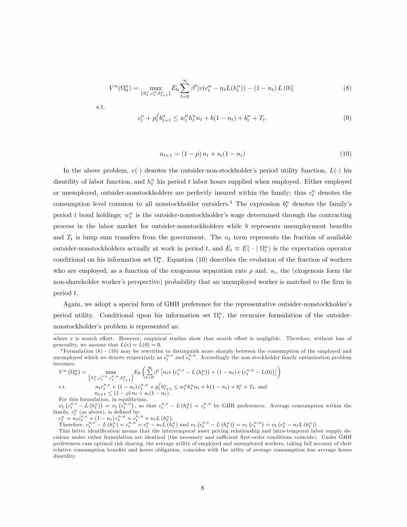
V n(n0 ) = maxfhnt ;cnt ;bnt+1g

E0

1Xt=0

�t[v(cnt � ntL(hnt ))� (1� nt)L (0)] (8)

s.t.

cnt + pft bnt+1 � wnt h

nt nt + b(1� nt) + bnt + Tt: (9)

nt+1 = (1� �)nt + st(1� nt) (10)

In the above problem, v(�) denotes the outsider-non-stockholder�s period utility function, L(�) hisdisutility of labor function, and hnt his period t labor hours supplied when employed. Either employed

or unemployed, outsider-nonstockholders are perfectly insured within the family; thus cnt denotes the

consumption level common to all nonstockholder outsiders.4 The expression bnt denotes the family�s

period t bond holdings; wnt is the outsider-nonstockholder�s wage determined through the contracting

process in the labor market for outsider-nonstockholders while b represents unemployment bene�ts

and Tt is lump sum transfers from the government. The nt term represents the fraction of available

outsider-nonstockholders actually at work in period t; and Et � E( � j nt ) is the expectation operatorconditional on his information set nt . Equation (10) describes the evolution of the fraction of workers

who are employed, as a function of the exogenous separation rate � and, st, the (exogenous form the

non-shareholder worker�s perspective) probability that an unemployed worker is matched to the �rm in

period t.

Again, we adopt a special form of GHH preference for the representative outsider-nonstockholder�s

period utility. Conditional upon his information set nt , the recursive formulation of the outsider-

nonstockholder�s problem is represented as:

where e is search e¤ort. However, empirical studies show that search e¤ort is negligible. Therefore, without loss ofgenerality, we assume that L(e) = L(0) = 0.

4Formulation (8) - (10) may be rewritten to distinguish more sharply between the consumption of the employed andunemployed which we denote respectively as cn;et and cn;ut . Accordingly the non-stockholder family optimization problembecomes:

V n�n0�= maxn

hnt ;cn;et ;c

n;ut ;bnt+1

oE0� 1Pt=0

�t�ntv

�cn;et � L (hnt )

�+ (1� nt) v

�cn;ut � L(0)

���s.t. ntc

n;et + (1� nt) c

n;ut + pft b

nt+1 � wnt h

nt nt + b (1� nt) + bnt + Tt, and

nt+1 � (1� �)nt + st(1� nt).For this formulation, in equilibrium,v1�cn;et � L (hnt )

�= v1

�cn;ut

�; so that cn;et � L (hnt ) = cn;ut by GHH preferences. Average consumption within the

family, cnt (as above), is de�ned by:cnt = ntc

n;et + (1� nt) c

n;ut = cn;ut + ntL (hnt ).

Therefore, cn;et � L (hnt ) = cn;ut = cnt � ntL (hnt ) and v1�cn;et � L (hnt )

�= v1

�cn;ut

�= v1 (cnt � ntL (hnt )) :

This latter identi�cation means that the intertemporal asset pricing relationship and intra-temporal labor supply de-cisions under either formulation are identical (the necessary and su¢ cient �rst-order conditions coincide). Under GHHpreferences cum optimal risk sharing, the average utility of employed and unemployed workers, taking full account of theirrelative consumption bene�ts and hours obligation, coincides with the utlity of average consumption less average hoursdisutility.

8

V n(nt ) = maxfcnt ;bnt+1;hnt g

2664v(cnt � ntL(hnt ))

+�nt (bnt + w

nt h

nt nt + b(1� nt)� p

ft bnt+1 � cnt )

+�E(V n(nt+1) j nt )] 5

3775 (11)

where �nt is the Lagrange multiplier associated with the outsider-nonstockholder�s budget constraint (9).

The solution to the above recursive problem (11) is characterized by the necessary and su¢ cient �rst

order conditions:

vc(cnt � ntL(hnt )) = �nt (12)

wnt = L1(hnt ) (13)

pft = �E(v1(c

nt+1 � nt+1L(hnt+1)))v1(cnt � ntL(hnt ))

j nt )]: (14)

Note that outsider-nonstockholders� hours are supplied under the condition that the (hourly) wage

equals the marginal rate of substitution of consumption for leisure.

We next describe the functioning of this labor market and its wage determination process.

2.3 Search in the labor market for outsider-nonstockholders

There is one in�nitely lived representative �rm that behaves competitively.6 The �rm hires nt outsider-

nonstockholders from the outsider�s labor market in period t. The �rm also posts �t vacancies in order

to attract new outsiders for its period t+1 production. The total number of unemployed outsiders who

search for a job in period t, ut, is given by:

ut � 1� nt:

Based on the Mortensen and Pissarides search theory, we postulate that the following matching

technology exists in the labor market for outsiders in period t. The exponents � and (1� �) describe,respectively, the elasticity of matches with respect to vacancies and unemployment.

M(�t; 1� nt) = �m��t (1� nt)1��,

where �m is a scale parameter, and mt � M(�t; 1 � nt) represents "matches," the number of newly

hired outsiders.

5nt =nwt; nt; st; bt; P

ft

o. In addition, there is no multipler for equation (10) as it contains no decision variables.

6Equivalently, it can be assumed that there is a continuum of in�nitely lived identical competitive �rms distributed onthe unit interval [0; 1].

9

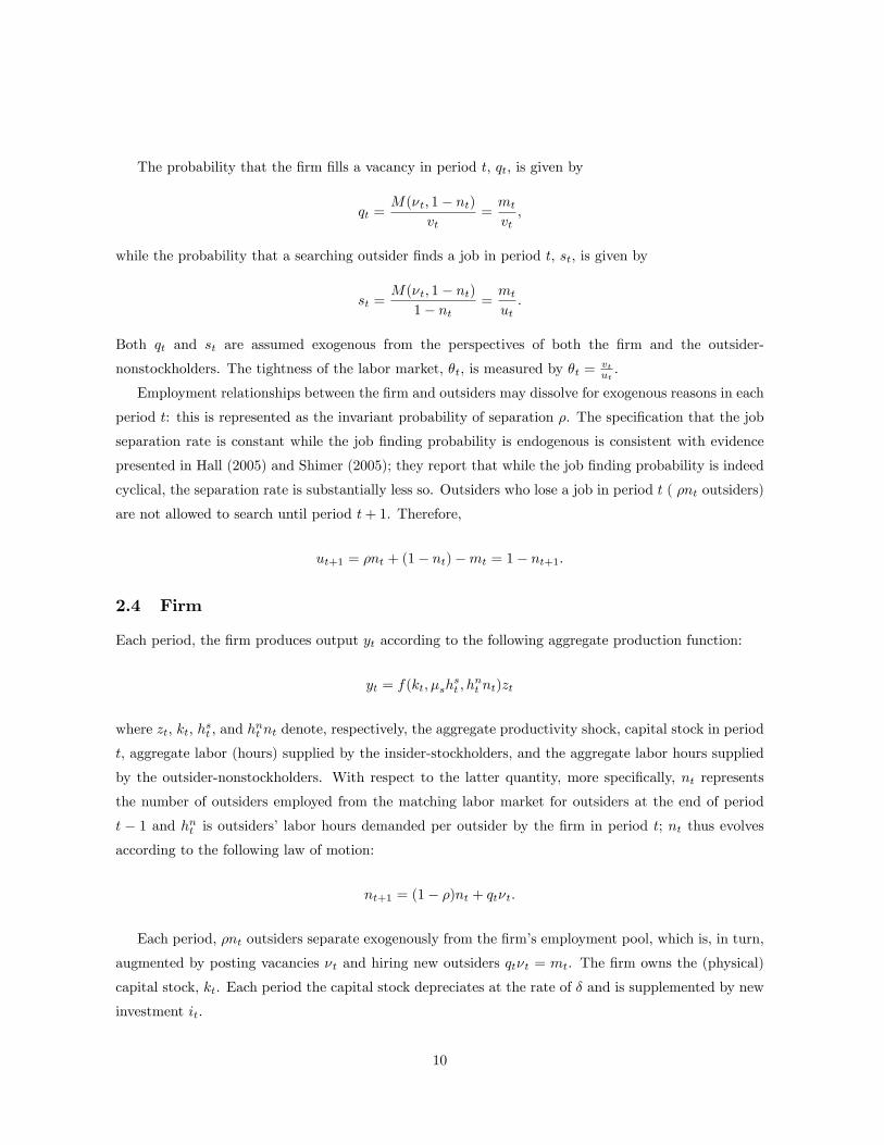
The probability that the �rm �lls a vacancy in period t, qt, is given by

qt =M(�t; 1� nt)

vt=mt

vt,

while the probability that a searching outsider �nds a job in period t, st, is given by

st =M(�t; 1� nt)

1� nt=mt

ut.

Both qt and st are assumed exogenous from the perspectives of both the �rm and the outsider-

nonstockholders. The tightness of the labor market, �t, is measured by �t = vtut.

Employment relationships between the �rm and outsiders may dissolve for exogenous reasons in each

period t: this is represented as the invariant probability of separation �. The speci�cation that the job

separation rate is constant while the job �nding probability is endogenous is consistent with evidence

presented in Hall (2005) and Shimer (2005); they report that while the job �nding probability is indeed

cyclical, the separation rate is substantially less so. Outsiders who lose a job in period t ( �nt outsiders)

are not allowed to search until period t+ 1. Therefore,

ut+1 = �nt + (1� nt)�mt = 1� nt+1:

2.4 Firm

Each period, the �rm produces output yt according to the following aggregate production function:

yt = f(kt; �shst ; h

nt nt)zt

where zt, kt, hst , and hnt nt denote, respectively, the aggregate productivity shock, capital stock in period

t, aggregate labor (hours) supplied by the insider-stockholders, and the aggregate labor hours supplied

by the outsider-nonstockholders. With respect to the latter quantity, more speci�cally, nt represents

the number of outsiders employed from the matching labor market for outsiders at the end of period

t � 1 and hnt is outsiders�labor hours demanded per outsider by the �rm in period t; nt thus evolves

according to the following law of motion:

nt+1 = (1� �)nt + qt�t:

Each period, �nt outsiders separate exogenously from the �rm�s employment pool, which is, in turn,

augmented by posting vacancies �t and hiring new outsiders qt�t = mt. The �rm owns the (physical)

capital stock, kt. Each period the capital stock depreciates at the rate of � and is supplemented by new

investment it.

10

Two costs of adjusting the �rm�s capital stock and the labor force of outsider-nonstockholders are next

introduced. Merz and Yashiv (2007) report that the simultaneous introduction of these two adjustment

costs empirically a¤ects the market value of the �rm; ignoring either cost does not match with their

empirical evidence.7

Capital adjustment costs have a long tradition in the investment theory literature. Such costs form

a wedge between the shadow price of capital installed within the �rm and the price of an additional unit

of capital. We replace the standard capital-accumulation technology with the speci�cation employed in

Jermann (1998):

kt+1 = (1� �)kt +G(itkt)kt

where the adjustment cost function G(�) is given by

G(itkt) =

a1

1� 1�

(itkt)1�

1� + a2

and a1 and a2 are chosen so that G(�) = �, and G0(�) = 1. With these identi�cations, the elasticity

parameter � � � 1G00(�)� > 0 is independent of the determination of the model�s steady-state equilibrium,

i.e. the steady state is not a¤ected by the positive value �; � = 1 corresponds to the benchmark case

of no adjustment costs. This speci�cation enables Tobin�s q to vary by di¤erentiating between the

(shadow) prices of the installed capital and the new investment good prices.

Second, we introduce a cost of adjusting employment. These costs in�uence the rate at which the

�rm adds new workers to its existing labor force. We replace the standard assumption of �xed costs of

posting a vacancy with quadratic labor adjustment costs, as in Gertler and Trigari (2009). De�ning the

hiring rate xt as the ratio of new hires qt�t to the existing workforce of outsider-nonstockholders, the

quadratic adjustment costs of the employment size of outsider-nonstockholders is given by

�

2x2tnt

where xt � qt�tnt

= new hiresexisting workforce � hiring rate and � is a constant vacancy cost.

The (�nancial) capital structure of the representative �rm consists of one perfectly divisible equity

share and one-period risk-free bonds: the �rm is not only equity-�nanced but also �nanced by the

issuance of one period default free (risk free) corporate bonds at price pft . The total supply of corporate

bonds is constant over time and equals a fraction ' of the average capital stock owned by the �rm as in

Danthine and Donaldson (2002). In each period, the �rm makes net interest payments ('�k � pft '�k) to

bondholders. Since the Modigliani-Miller theorem holds true in this framework, the existence of leverage

has no e¤ect on real allocations8 .7 [New footnote here]8We can verify this property by solving the model with and without leverage: real allocations are identical. The

11

The �rm�s decision problem is to maximize its pre-dividend stock market value dt + pet on a period-

by-period basis given its information set ft = f (kt; �t; qt; nt):

maxfit;hst ;xtg

dt + pet � dt + E(��

st;t+1(p

et+1 + dt+1) j

ft ) (15)

s.t. dt � f(kt; �shst ; h

nt nt)zt � it � wst�shst � wnt hnt nt �

�

2x2tnt � '�k + p

ft '�k

kt+1 = (1� �)kt +G(itkt)kt

nt+1 = (1� �)nt + qt�t . 9

In the above problem, �st;t+1 is the marginal rate of substitution of the insider-stockholders, wst is their

competitive wage and wnt is the Nash bargaining wage for outsider-nonstockholders (speci�ed later).

Letting V f (ft ) � dt + pst , the recursive representation of the �rm�s problem is written as:

V f (ft ) = dt + �E(�st;t+1V

f (ft+1) j ft ):

The necessary and su¢ cient �rst-order condition for the �rm�s optimal investment decision is given

by:

it : (�1) + �E(�st;t+1Vfkt+1

j ft )@kt+1@it

= 0:

By the envelope theorem,

kt :@V f (ft )

@kt= f1(kt; �sh

st ; h

nt nt)zt + �E(�

st;t+1V

fkt+1

j ft )@kt+1@kt

= 0:

The investment Euler equation is thus represented as:

1 = �E(�st;t+1G0(itkt)[f1(kt+1; �sh

st+1; h

nt+1nt+1)zt+1 +

(1� �) +G( it+1kt+1)

G0( it+1kt+1)

� it+1kt+1

] j ft ): (16)

The �rst-order condition for the �rm �s optimal hiring decision of insiders is given by

hst : wst = f2(kt; �sh

st ; h

nt nt)zt; (17)

fundamental reason behind this neutral Modigliani-Miller outcome is that the �rm�s crucial intertemporal decisons are allin accord with the intertemporal marginal rate of substitution of the insider-stockholders; i.e. there is no agency problembetween �rm owners and managers in this environment. It turns out that the absence of corporate governance problemsis important to deriving Nash wage bargaining between capitalists and workers.

9Note that to choose the hiring rate xt is to choose the number of vacancies vt.

12

while the �rst-order condition for the �rm�s optimal hiring rate for outsiders is given by

xt : �xt = �Et�st;t+1Jt+1 (18)

where Jt � @V f (t)@nt

is the �rm�s shadow value of one additional outsider hired.

2.5 Characterizing the Nash bargaining problem10

In this section, we formalize the Nash wage bargaining process between the �rm and the outsider-

nonstockholders. In this environment, there exists a wedge between capital owners�intertemporal mar-

ginal rate of substitution (IMRS) and workers�IMRS: the �rm is the representative of the capital owners

(insider-nonstockholders), not workers. Nevertheless, we show that the Nash wage bargaining solution

can be constructed in a tractable way. In other words, the �rm�s matching surplus and the outsider-

nonstockholder�s employment and unemployment values can be de�ned in terms of current consumption

so as to make them consistent with the �rm�s shadow value of one added worker and the outsider-

nonstockholder�s value of becoming employed, respectively. What emerges from this representation of

the Nash bargaining problem in terms of current consumption is a tractable form of Nash bargaining

which nests, as the special case, the standard Nash bargaining wage in the representative agent analogue.

Firm�s shadow value of hiring one outsider Presuming that the �rm�s decision variables are

chosen optimally, the �rm�s pre-dividend stock market value V f (ft ) � V ft � dt+pet can be represented

recursively as follows:

V ft = dt + pet

= dt + �E(�st;t+1(p

et+1 + dt+1) j

ft )

= dt + �E(�st;t+1V

ft+1 j

ft )

Let us be more speci�c about the structure of Jt =@V f(ft )@nt

, the per-capita value to the �rm of

hiring one outsider in period t:

Jt = hnt f3(kt; �shst ; h

nt nt)zt � wnt hnt +

�

2x2t + (1� �)�Et�st;t+1Jt+1

where hnt f3(kt; �shst ; h

nt nt)zt de�nes the "extensive marginal product of outsiders�labor."

11

10This model is essentially the same as one in which shareholder-workers directly manage the �rm, as though it werea private company. As �rm owners, they trade bonds with their workers. There is no explicit stock market under thisformulation, and no MRSs to be conveyed by the shareholders to the �rm as in the present "more realistic" formulation.Accordingly, the return on equity is measured as the marginal product of capital. The present formulation is moreconsistent with the recent literature.11 In the matching labour market for outsiders, we distinguish between the "extensive marginal product of outsiders�

labour" and the "intensively marginal product of insiders� labour." Similarly, the intensive marginal product of labour,

13

The �rst-order condition for the hiring rate equates the marginal cost of adding an outsider with

discounted marginal bene�t:

�xt = �Et�st;t+1Jt+1: (19)

Note that condition (19) is identical to the �rm�s optimal hiring decision for outsiders (18).

Using the de�nition of Jt; we have the following equivalent optimality condition:

�xt = �Et�t;t+1[hnt+1f3(kt+1; �sh

st+1; h

nt+1nt+1)zt+1 � wnt+1hnt+1 +

�

2x2t+1 + (1� �)�xt+1]:

Distribution risk In equilibrium, the extent of partial risk sharing that results from insider-stockholders

and outsider-nonstockholders interacting in the bond market will in�uence the outcome of the Nash wage

bargaining process and will in turn be a¤ected by it. To measure the cumulative e¤ect we introduce

the ratio between the insider-stockholder�s marginal utility and the outsider-nonstockholder�s marginal

utility:

�t �uc((c

st � �cst�1 �H(hst ))vc(cnt � ntL(hnt ))

=�st�nt. (20)

as characterizing the extent of risk-sharing between these two groups. If �t is constant across time and

in all states, the relation (20) coincides with the e¢ cient risk-sharing condition. Alternatively, suppose

that �t is constant across period t states for each t but time-varying.12 A larger �t is evidence of a

greater share of aggregate income to workers while a smaller �t suggests a greater share to capital owners

(shareholders). Suppose, in addition, that �t is time-varying and countercyclical over the business cycle.

This countercyclicality means that when a high-productivity state is realized, a smaller �t is realized

and insider-stockholders (capital owners) reap most of the bene�ts from that high productivity state;

in comparison, when a low-productivity state is realized, a greater share of aggregate income goes to

outsider-nonstockholders, i.e. the normally low payment to capital owners is further reduced by labor�s

priority claim on output. Accordingly, the countercyclicality of �t captures the idea that the shares of

income going to labor and capital are not equally risky and that insider-stockholders, via the institution

of the �rm, are partially insuring the outsider-nonstockholders. This "distribution risk" (variation in

�t) is largely borne by the �rm and its owners.13 ; 14

MPLhnt , is de�ned as@yt@hnt

= ntztf3(kt; �shst � 1; hnt � nt):

12Here the optimal contract is not necessarily optimal in the Pareto sense. In this case, relation (20) is reduced to theoptimality condition of the Boldrin-Horvath (1995) type optimal contract.13Empirically, labour�s share is much less risky than the share going to capital; labour�s claim on output is largely �xed

and negotiated prior to the actual realization of the output.14 In an earlier paper, Danthine and Donaldson (2002) posit that the observed variations in factor income shares are

the result of exogenous changes in this ratio �t which they refer to as distribution risk (hereafter we call the ratio �tdistribution risk). This risk is assumed to be uninsurable. They view �t as capturing the relative bargaining power of thetwo parties at the time the contract is negotiated. The assumed countercyclicality of this distribution risk guarantees thatlabour�s share is much less risky than the share going to capital. In comparison, our endogenous distribution risk measure

14

We make no a priori assumption either about the cyclicality of distribution risk or about the source of

this risk; rather, distribution risk in this economy is generated entirely endogenously in equilibrium: our

economy features one source of uncertainty resulting from systemic risk (the economy-wide productivity

shock). It turns out, however, that distribution risk (de�ned as per (20)) is indeed countercyclical

over the business cycle in the present model. Furthermore, our Nash bargaining wage contract between

capitalists (insider-stockholders) and laborers (outsider-nonstockholders) precisely identi�es distribution

risk �t with the balance of "bargaining power" between capitalists and laborers. As a result, we provide

a structural speci�cation of the source of distribution risk.

Outsider-nonstockholder�s shadow value The present discounted value to an outsider of employ-

ment in terms of current consumption in period t, Wt, is de�ned recursively as

Wt = wnt hnt + (1� �)�Et�nt;t+1Wt+1 + ��Et�

nt;t+1Ut+1

where �nt;t+1 ��nt+1�nt

is the outsider-nonstockholder�s IMRS.

We recursively de�ne Ut as the present discounted value to an outsider of unemployment in terms

of current consumption in period t:

Ut = L(hnt ) + b+ st�Et�nt;t+1Wt+1 + (1� st)�Et�nt;t+1Ut+1:

Here, the value of being unemployed depends upon the outsider�s current disutility of supplying hours

L(hnt ) (measured in units of �nal good consumption) , his unemployment bene�ts b, and the likelihood

of his being employed or unemployed next period; an unemployed outsider has a chance of �nding a

new job, st.

The outsider-nonstockholder�s matching shadow value in terms of �nal good consumption, Snt , is

therefore de�ned as the di¤erence between the employment value and the unemployment value:

Snt � Wt � Ut (21)

= (wnt hnt � L(hnt )� b) + (1� �� st)�Et�nt;t+1Snt+1:

Alternatively, the matching shadow value Snt can also be derived from the marginal bene�t of a

outsider-nonstockholder family from having an additional family member employed. The recursive

is very di¤erent.

15

representation of the outsider-nonstockholder�s problem is:

V nt � V n(nt ) = maxfbnt+1;hnt g

2664v(cnt � ntL(hnt )� (1� nt)L(0))

+�nt (wnt h

nt nt + (1� nt)b+ bnt � p

ft bnt+1 � cnt )

+�E(V n(nt+1) j nt )

3775 (22)

s.t.

nt+1 = (1� �)nt + st(1� nt):

The marginal bene�t of one hired worker, V nnt �@V nt@nt

, can be obtained by applying the Envelope theorem

to representation (22):

@V nt@nt

= wnt hnt �

nt � (L(hnt ) + b)�nt + �Et

@V nt+1@nt+1

@nt+1@nt

where @nt+1@nt

= (1� �� st).De�ne the outsider-nonstockholder�s shadow value to the �rm of one hired worker, Snt , as

Snt � 1

�nt

@V nt@nt

(23)

= (wnt hnt � L(hnt )� b) + (1� �� st)�Et

�nt+1�nt

Snt+1:

It follows immediately that the above shadow value, Snt in (23), exactly coincides with the outsider-

nonstockholder�s matching shadow value (21).

Nash wage bargaining Before formalizing the Nash bargaining wage contract between insider-

stockholders and outsider-nonstockholders, �rst note that the �rm�s intertemporal decisions are all

in accord with the intertemporal marginal rate of substitution of the insider-stockholders: there is

no agency problem between �rm owners and managers in this environment. Accordingly, the �rm�s

matching surplus can thus be identi�ed with the marginal bene�t to the representative shareholder of

adding one outsider-nonstockholder worker. In other words, the �rm�s matching surplus, denoted V snt ,

can be formulated as:

V snt �@V st@nt

where V st � V s(st ) is the value function of insider-stockholders.

As shown in the previous section, the outsider-nonstockholder�s matching surplus, V nnt , can be readily

identi�ed with the marginal bene�t (to the family) of one additional worker being hired:

V nnt �@V nt@nt

:

16

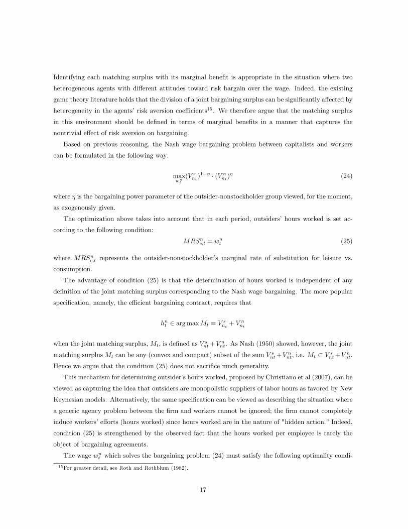
Identifying each matching surplus with its marginal bene�t is appropriate in the situation where two

heterogeneous agents with di¤erent attitudes toward risk bargain over the wage. Indeed, the existing

game theory literature holds that the division of a joint bargaining surplus can be signi�cantly a¤ected by

heterogeneity in the agents�risk aversion coe¢ cients15 . We therefore argue that the matching surplus

in this environment should be de�ned in terms of marginal bene�ts in a manner that captures the

nontrivial e¤ect of risk aversion on bargaining.

Based on previous reasoning, the Nash wage bargaining problem between capitalists and workers

can be formulated in the following way:

maxwnt(V snt)

1�� � (V nnt)� (24)

where � is the bargaining power parameter of the outsider-nonstockholder group viewed, for the moment,

as exogenously given.

The optimization above takes into account that in each period, outsiders�hours worked is set ac-

cording to the following condition:

MRSnc;l = wnt (25)

where MRSnc;l represents the outsider-nonstockholder�s marginal rate of substitution for leisure vs.

consumption.

The advantage of condition (25) is that the determination of hours worked is independent of any

de�nition of the joint matching surplus corresponding to the Nash wage bargaining. The more popular

speci�cation, namely, the e¢ cient bargaining contract, requires that

hnt 2 argmaxMt � V snt + Vnnt

when the joint matching surplus, Mt, is de�ned as V snt+Vnnt. As Nash (1950) showed, however, the joint

matching surplusMt can be any (convex and compact) subset of the sum V snt+Vnnt, i.e. Mt � V snt+V

nnt.

Hence we argue that the condition (25) does not sacri�ce much generality.

This mechanism for determining outsider�s hours worked, proposed by Christiano et al (2007), can be

viewed as capturing the idea that outsiders are monopolistic suppliers of labor hours as favored by New

Keynesian models. Alternatively, the same speci�cation can be viewed as describing the situation where

a generic agency problem between the �rm and workers cannot be ignored; the �rm cannot completely

induce workers�e¤orts (hours worked) since hours worked are in the nature of "hidden action." Indeed,

condition (25) is strengthened by the observed fact that the hours worked per employee is rarely the

object of bargaining agreements.

The wage wnt which solves the bargaining problem (24) must satisfy the following optimality condi-

15For greater detail, see Roth and Rothblum (1982).

17

tion16 :

�V snt = (1� �)Vnnt . (26)

Condition (26) can be rewritten as:

��stJt = (1� �)�nt (Wt � Ut): (27)

using the substitutions V snt = �stJt and V nnt = �nt (Wt � Ut). A standard calculation based on the

condition (27) guarantees that the Nash bargaining wage between two heterogeneous groups is given by

wnt =(1� �) 1�t

(1� �) 1�t + �[L(hnt ) + b� Fnt ]

hnt+

�

(1� �) 1�t + �[hnt f3(kt; �sh

st ; h

nt nt)zt +

�2x

2t + F

st ]

hnt(28)

where Fnt � �(1���st)Et�nt+1�nt(Wt+1�Ut+1) and F st � �(1��)Et

�st+1�st

Jt+1 denote, respectively, the fu-

ture net expected welfare bene�ts to the outsider-nonstockholders and to the �rm (insider-stockholders)

from one addidtional employed worker. By the very presence of the term �t in expression (28) it is

apparent that the �nancial market structure in�uences Nash bargaining wage determination.

Letting �t � �(1��) 1

�t+�, the solution (28) can be rewritten as:

wnt = (1� �t)[L(hnt ) + b� Fnt ]

hnt+ �t

[hnt f3(kt; �shst ; h

nt nt)zt +

�2x

2t + F

st ]

hnt: (29)

This Nash bargained wage (29) is seen to nest the standard bargaining wage under the representative

agent regime as a special case. In the case of the representative-agent construct, markets are complete so

that �t is equal to 1, and the solution (29) is reduced to the standard Nash bargaining solution (�t = �).

This observation highlights the signi�cant role of limited asset market participation in generating variable

distribution risk �t, and thus variable nt.

More important, it can be shown that up to a �rst-order approximation,

�t = (constant) � �t:17

In other words, the notion of distribution risk can be identi�ed with a Nash bargaining power shock up to

a �rst-order approximation. Later it will be shown that distribution risk in this sense is countercyclical

over the business cycle. Indeed, the countercyclicality of distribution risk in this model will play the key

role in generating the unemployment �uctuations over the business cycle with the coveted properties:

the countercyclicality of the distribution risk creates excessively smooth wages that induce a �xed wage

income e¤ect (the operating leverage e¤ect), which encourages the observed volatility of key labor market

16This condition is called the constant surplus sharing rule.17A ^on a variable denotes log deviations from the corresponding steady-state value.

18

variables of interest. Our sense of distribution risk is thus exactly the same as the Nash bargaining power

shock Shimer took into account without invoking its source (Shimer, 2005). In fact, our work may be

viewed as providing microfoundations for the Shimer�s ad hoc Nash bargaining power shock. Note that

the only exogenous driving force in our economy is an aggregate productivity shock which induces the

countercyclicality of our distribution risk. This may be seen as a direct answer to Shimer�s unanswered

question, as stated in Shimer (2005): "It seems plausible that a model with a combination of wages

and labor productivity shocks could generate the observed behavior of unemployment, vacancies, and real

wages... the answered question is what exactly a wage shock is." Our model is a particular instance of

what Shimer seeks. It also provides micro foundations for the exogenous distribution risk assumed in

Danthine and Donaldson (2002).

2.6 Equilibrium

In this economy, market clearing requires that for all t,

et =

Zestd{ = 1;

��k =

Zbstd{ +

Zbnt d!;

ct =

Zcstd{ +

Zcnt d!;

yt = ct + it +�

2xt2nt;

where { and ! respectively stand for the measure of insider-stockholders and the measure of outsider-

nonstockholders. Lump sum transfers are taxed to balance the government budget constraint:

Tt + (1� nt)b = 0:

We de�ne the equilibrium as follows:

De�nition 1 Under the above market-clearing conditions, a decentralized stationary recursive equilib-

rium is de�ned as: a set of decision rules fcst (�); cnt (�);hst (�); hnt (�); et+1(�); it(�); ht(�); �t(�)g and a setof wage and price functions fwst (�); wnt (�); pet (�); p

ft ; dt(�)g given the information set of aggregate states

= fkt; nt;�tg such that (i) fcst (�); hst (�); et+1(�); bst+1(�)g solves the intertemporal problem (1) given

the information set st (ii)fcnt (�); hnt (�); bnt+1g solves the outsider-nonstockholder�s intertemporal problem(8) given his information set nt (iii)fwnt (�)g satis�es the optimality condition (27) (iv) fit(�); xt(�)gsolves the �rm�s intertemporal problem given the information set f (15) (vi) wst (�) satis�es the con-dition (17) (vii)fpet (�); dt(�)g satis�es the Lucas asset pricing equations (6), while f p

ft (�)g satis�es the

19

equations (7) and (14) (ix) The economy follows two laws of motion: kt+1 = (1 � �)kt + G( itkt )kt and

nt+1 = (1� �)nt + qtvt. Rational expectations are assumed for all agents.

2.7 Asset Pricing

Under the decentralized stationary recursive equilibrium de�ned in Section 3.8, it is possible to de�ne

and compute equilibrium asset prices and returns. Using the dividend series, the conditional price pe(t)

of an equity security is recursively computed according to the Lucas�(1978a) asset pricing equation:

pe(t) = �E(�st+1�st

[pe(t+1) + d(t+1)] j t);

where t = fkt; nt; ztg is the aggregate state of economy and �st = uc(cs(t); h

s(t)) is the shareholder-

worker�s equilibrium marginal utility.

Using these prices, the time series of equity returns is computed in the conventional way:

Ret;t+1 =pe(t+1) + d(t+1)

pe(t)� 1.

In a similar fashion, the price of a one-period risk-free real bond is given by

pf (t) = �E(�t+1�t

j t)

where �t = uc(cs(t); h

s(t)) or �t = vc(cn(t); h

n(t)). Note that the risk free bond is available to

all households. The one period risk-free rate of return, Rft , is then computed using

Rft =1

pf (t)� 1:

Given the aggregate state t = fkt; nt; ztg , the conditional term structure fRft;ng can also be derived.Let pfn(t) = �nE(�t+n�t

j t) denote the price of a risk free discount bond in period t that pays oneunit of consumption in period t+ n. Then

nRft;n

ois de�ned according to

Rft;n = [1

pfn(t)]1=n � 1;

Appendix 1 details the strategy for computing these various rates.

20

3 Calibration

In this paper, the business cycle is characterized as deviations from a Hodrick-Prescott �ltered trend.

The time unit of the model is three months. To match the US Solow residual we calibrate the process

for aggregate productivity shocks to match the quarterly AR(1) process found by Cooley and Prescott

(1995). The productivity shock zt thus evolves according to the law of motion:

log zt+1 = 0:95 log zt + �t+1

where � is distributed normally, with mean zero and standard deviation ��; in what follows, the standard

deviation of technology shock �� will be chosen by a procedure of "hyperparameter search."

For all simulation runs, the production function employed is the customary Cobb-Douglas function

ztf(kt; hst � 1; hnt � nt) = ztMk�t ((�sh

st � 1)�(hnt � nt)1��)1��

where � � �s1+�s

.

The parameter M serves as a scale parameter, while � = �s1+�s

and 1� � are, respectively, the nor-

malized measures of insider-stockholders and the outsider-nonstockholders. To allow for debt-�nancing

while imposing the constraint that corporate debt is risk-free, we scale our production technology by set-

ting M = 1:25. This makes the average output high enough to guarantee a uniformly positive dividend

in all states of nature for empirically relevant calibrations of the �rm�s debt level. Following Guvenen

(2003), the stock market participation rate, �s, is set to be 25 percent, so that � equals 0.20.

The parameter � is typically calibrated to reproduce the observed share of capital in total value

added. We adopt the most commonly used value, 0:36. The subjective discount factor � is �xed at

� = 0:99, corresponding to a steady state return on capital of 4%. Following Kydland and Prescott

(1982), the quarterly capital depreciation rate � is 0:020.

The model economy assumes that search and matching frictions characterize the labor market only

for outsider-nonstockholders. Therefore, we calibrate the labor market for outsider-nonstockholders

using standard parameters for labor market search and matching.

The empirical literature provides several estimates of the US worker separation rate. We follow

Davis, Haltiwanger and Schuh (1996) and �x the quarterly separation rate � at 8 percent. According to

Petronglo and Pissarides (2001), the elasticity of matches to unemployment of outsiders 1�� falls withinthe range of plausible values of 0.5 to 0.7. We set 1� � to be 0.5. The mean quarterly unemployment

rate of the model economy is set to 6%, which is customary in the literature (e.g. Merz (1995) and

Christo¤el and Kuester (2008)). Following, e.g. Cooley and Quadrini (1999), the steady state value

of the vacancy-�lling probability �q is set to be 0.7. The existing literature mostly suggests that the

bargaining power parameter � is equal to 0.5; we follow suit.

21

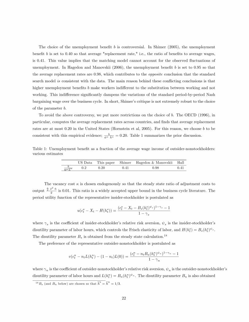
The choice of the unemployment bene�t b is controversial. In Shimer (2005), the unemployment

bene�t b is set to 0.40 so that average "replacement rate," i.e., the ratio of bene�ts to average wages,

is 0.41. This value implies that the matching model cannot account for the observed �uctuations of

unemployment. In Hagedon and Manovskii (2006), the unemployment bene�t b is set to 0.95 so that

the average replacement rates are 0.98, which contributes to the opposite conclusion that the standard

search model is consistent with the data. The main reason behind these con�icting conclusions is that

higher unemployment bene�ts b make workers indi¤erent to the substitution between working and not

working. This indi¤erence signi�cantly dampens the variations of the standard period-by-period Nash

bargaining wage over the business cycle. In short, Shimer�s critique is not extremely robust to the choice

of the parameter b.

To avoid the above controversy, we put more restrictions on the choice of b. The OECD (1996), in

particular, computes the average replacement rates across countries, and �nds that average replacement

rates are at most 0.20 in the United States (Hornstein et al, 2005). For this reason, we choose b to be

consistent with this empirical evidence; b�wn �hn

= 0:20. Table 1 summarizes the prior discussion.

Table 1: Unemployment bene�t as a fraction of the average wage income of outsider-nonstockholders:various estimates

US Data This paper Shimer Hagedon & Manovskii Hallb

wnhn 0.2 0.20 0.41 0.98 0.41

The vacancy cost � is chosen endogenously so that the steady state ratio of adjustment costs to

output�2 �x2 �n

�y is 0.01. This ratio is a widely accepted upper bound in the business cycle literature. The

period utility function of the representative insider-stockholder is postulated as

u(cst �Xt �H(hst )) =(cst �Xt �Bs(hst ) s)1� s � 1

1� s

where s is the coe¢ cient of insider-stockholder�s relative risk aversion, s is the insider-stockholder�s

disutility parameter of labor hours, which controls the Frisch elasticity of labor, and H(hst ) = Bs(hst ) s .

The disutility parameter Bs is obtained from the steady state calculation.18

The preference of the representative outsider-nonstockholder is postulated as

v(cnt � ntL(hnt )� (1� nt)L(0)) =(cnt � ntBn(hnt ) n)1� n � 1

1� n

where n is the coe¢ cient of outsider-nonstockholder�s relative risk aversion, n is the outsider-nonstockholder�s

disutility parameter of labor hours and L(hnt ) = Bn(hnt ) n . The disutility parameter Bn is also obtained

18Bs (and Bn below) are chosen so that hs= h

n= 1=3.

22

from the steady state calculation. We assume that s is equal to n and s is equal to n with denot-

ing the economy-wide coe¢ cient of relative risk aversion (i.e. s = n � ) and as the economy-wide

disutility-of-labor parameter (i.e. s = n � ). With these identi�cations, none of the results cited

below can be attributed to di¤erential risk aversion.19

It is well known that empirical studies do not o¤er much precise guidance when it comes to calibrating

the habit formation parameter �, the capital adjustment cost � and the coe¢ cients of relative risk

aversion . It is also widely known that the standard deviation of the technology shock innovation, ��,

is di¢ cult to measure from available data since this number, usually identi�ed with the direct estimate

of the volatilty of Solow residual for the post war period, is signi�cantly a¤ected by measurement error.

Furthermore, a high value of �� suggests a probability of technological regress that is implausibly large.

Lastly, we add the disutility-of-labor parameter to our list of free parameters. Although it is believed

to be less than 0.5 (e.g., McCurdy (1981)), the estimate of the Frisch elasticity of labor supply is not

conclusive. Indeed, Imai and Kean (2004) recently estimated the Frisch elasticity of labor supply as 3.8,

which is much higher than what is generally believed.

The lack of clarity in parameter determination leads us to conduct a "hyperparameter search" for

the parameters that are free at this point (�, �, , , ��) to match a set of empirical targets of interest.

This amounts to minimizing an equally weighted quadratic criterion function written in the deviation

from each empirical target in the manner of Jermann (1998). For the baseline calibration, we choose the

free parameters (�, �, , , ��) to match four empirical targets: (i) the relative standard deviation of

unemployment (a ratio of unemployment volatility to to output volatility) (ii) the risk-free rate volatility

(iii) the mean risk-free rate and (iv) the equity premium. Practically, we restrict our hyperparameter

search to a grid of values for � 2 [0; 0:9]; � 2 [0:23;1); �� 2 [0:0037; 0:00712]; 2 [1; 2] and 2 [1; 7].These intervals encompass most estimates from the literature. For the baseline calibration, the minimum

is achieved for �� = 0:006; � = 0:9; � = 0:23; = 1:4 and = 3:6. A value of = 1:4 implies that the

Frisch elasticity of labor supply in this economy is 11:4�1 = 2:5 as in Jaimovich and Rebelo (2008). Our

Frisch elasticity of labor supply is thus higher than its traditional estimate but is less than the Imai-

Kean estimate of 3.8. At 0.6%, the value of the innovation standard deviation is much smaller than the

values used by other macro-asset pricing models, e.g., Boldrin, Christiano and Fisher (2001), Danthine

and Donaldson (2002), and Guvenen (2003). These models value the innovation standard deviation per

quarter at close to 2%. For instance, Boldrin, Christiano and Fisher (2001) use permanent shocks with a

standard deviation of 1.8% per quarter. Indeed, our value is even smaller than the direct estimate of the

volatility of Solow residuals for the post war period, which is about 0.7%. We view a reduced reliance

on large technology disturbances as a favorable attribute of the model. The model is then solved using

the log-linearization methods widely employed in the business cycle literature. Log-normal formulae are

19This being said, we recognize that habit formation makes the insider-stockholder e¤ectively more risk averse than theoutsider-nonstockholder.

23

applied to price the relevant asset returns (see e.g. Uhlig (1999) or Jermann (1998) and Appendix 1).20 ;

21

4 Results

4.1 Model Results

Reassessing Shimer�s critique: Before reporting the quantitative results for the baseline model,

we raise several issues as to how Shimer�s critique might be best represented in (real) business cycle

models with labor-market search, and modify it accordingly. In his seminal paper, Shimer claims that

the incorporation of the standard search model into a real business cycle framework with intertemporal

substitution of leisure, capital accumulation, and other extensions such as the Merz (1995) or Andolfatto

(1996) models does not invalidate his critique. In his words, "Neither paper can match the negative

correlation between unemployment and vacancies, and both papers generate real wages that are too

�exible in response to productivity shocks" (p.45). Indeed, the Andolfatto model does not pass the

litmus test for the unemployment volatility puzzle Shimer raises: the model allows for a real wage that

is too �exible in response to productivity shocks with the result that the volatility of job vacancies

is too low to match its empirical counterpart. The Merz model, however, is hard to reject on this

basis alone. Table 2 in her paper shows that the model with �xed search intensity can replicate, quite

well, the basic stylized facts of labor market volatility; the wage is indeed rigid in terms of its relative

standard deviation (�w�y = 0:34) and the job vacancies are reasonably volatile (���y= 6:38). Both models

generate the negative correlation between unemployment and vacancies, although that correlation is

only weakly negative. Furthermore, it can be shown, up to a �rst-order approximation, that the Merz

model with �xed search intensity is isomorphic to the Andolfatto model with inelastic labor supply

of hours. The relative success of the Merz model (with �xed search intensity) in generating realistic

labor market statistics rides not only on wage stickiness, however, but also on the absence of variations

at the intensive margin. If the Merz model were to allow for variations at the intensive margin, its

ability to explain labor market volatility might be signi�cantly compromised; the representative �rm

now could substitute between hours per incumbent and hiring new workers. This substitution e¤ect is

not negligible over the business cycle, and explains why the Andofatto model performs so poorly on the

dimensions of the labor market business cycles: it allows both variations. Accordingly, a DSGE model�s

ability to resolve the unemployment volatility puzzle may depend upon the extent to which the labor

20Log-normal formulae can be found in the Appendix 1.21Given the generally accepted parameter choices from earlier macro studies and the parameters arising from the

hyperparameter search, we solve for all the steady state variables under the added assumption that n = :90; u = :10(unemployment); q = :7; and h

s= h

n= 1=3. These latter choices, commonplace in the literature, in turn determine Bs,

Bn, �n, etc.

24

supply of hours is elastic. To see if (quarterly) business cycle models with labor-market search can pass

a litmus test for the resolution of the unemployment volatility puzzle, a consideration of variations at

both the intensive margin and at the extensive margin is required.

We propose the following expansion of Shimer�s critique: (i) a quarterly business cycle model with

labor-market search must generate the absolute amplitude of the standard deviations of key variables in

the labor market activities as well as their relative magnitude vis-a-vis the standard deviation of output;

(ii) the model must allow for variations at the intensive margin and at the extensive margin simulta-

neously; and (iii) the negative correlation between unemployment and vacancies must be substantially

consistent with the data.22 The present model possesses all of these features.

Table 2 reports the second moments of endogenous aggregate variables as implied by the model,

namely unconditional standard deviations, and their contemporaneous correlation with output, alongside

the moments implied by the data. Table 4 reports the associated �nancial statistics implied by the

model alongside the �nancial statistics implied by the data (Mehra and Prescott, 1985). These results

are discussed below.

Table 2: Aggregate business cycle statistics: the baseline model

Business Cycle StatisticsVariable Meaning Std Std. to �y Corr. with y

Data(i) Model Data Model Data Modely output 1.59 1.47 - - - -c consumption 1.23 1.39 0.77 0.95 0.83 0.94i investment 4.87 2.22 3.06 1.51 0.91 0.86htotal total hours(i) 1.51 1.34 0.95 0.91 0.92 0.90h hours per worker(ii) 0.69 0.65 0.43 0.44 0.62 0.90hs hours per insider - 1.05 - 0.71 - 1.00hn hours per outsider - 0.56 - 0.38 - 0.87w wage(iii) 0.70 0.37 0.44 0.25 0.68 0.88ws wage per insider - 0.42 - 0.29 - 1.00wn wage per outsider - 0.23 - 0.16 - 0.87n employment 1.02 0.90 0.64 0.61 0.78 0.98u unemployment 11.01 10.36 6.92 7.05 �0.87 �0.84� vacancy 13.15 13.42 8.27 9.13 0.91 1.00� tightness 21.66 22.52 13.62 15.32 0.90 0.98(i) htott = �sh

st + nth

nt

(ii) ht = htott =nt + �s

(iii) wt = �swst + nt + w

nt

22The Merz model (with �xed search intensity) cannot pass Shimer�s (2005) litmus test for the resolution of the unem-ployment volatility puzzle. For instance, the amplitude of the standard deviation of vacancies is 6.85% while it empiricalcounterpart is around 13.15%; it also violates the condition (iii); the correlation between unemployment and vacancies(�0:15) falls short of its realism (�0:89); and the Merz model allows only for variations at the extensive margin.

25

Labor market volatility: The model reproduces the substantial �uctuations in the key variables of

labor market activity found in the data and emphasized by Shimer (2005) and Hall (2005). In particular,

in terms of the (absolute) volatility, the model comes remarkably close to the (absolute) volatilities of the

key labor market variables including unemployment u, vacancies �, and the market tightness measure

� � �u . This indicates that the propagation mechanism in this model economy is quite powerful since the

standard deviation of the productivity shock required to produce the observed variations in the labor

market variables of interest is 0.006, which is smaller than the direct estimate of the volatility of Solow

residuals from the post war data (about 0.007).

A distinguishing feature of our analysis is that we can disentangle the variations at the intensive

margin from the variations at the extensive margin. Fortunately, the model comes close to matching

precisely both the relative volatility of total hours (0.91 versus 0.95 in the data) and hours per worker

(0.44 versus 0.43 in the data). Although the correlation of hours per worker with output is too procycli-

cal, the model nevertheless captures the basic reality of the labor market as displayed in the data.23

As a consequence, the statistical behavior of employment also comes reasonably close to its empirical

counterpart.

Along the wage dimensions, however, the model somewhat overstates or understates the empirical

analogues: the real hourly wage is insu¢ ciently volatile and the contemporaneous correlation of hourly

wage with output is too procyclical. The departure of hourly wage volatility from its empirical mag-

nitude is in a way predictable. The Nash bargaining wage (wage per outsider) in this model economy

is signi�cantly a¤ected by the countercyclicality of endogenous distribution risk or Nash bargaining

power shock. This e¤ect dampens the variations in the Nash bargaining wage over the business cycle.

Indeed, the endogenous distribution risk is both highly volatile and strongly countercyclical, and thus

the equilibrium wage is less volatile over the business cycle. Nevertheless, the correlation of the wage

per outsider with output is still procyclical. The wage per insider is also less volatile, but its root

cause is quite di¤erent: it is determined by the marginal product of labor. This mechanism for wage

determination usually results in low volatility and strong procyclicality. In the indivisible RBC model of

Hansen (1985), where the wage coincides with the marginal product of labor, for example, the relative

standard deviation of the real wage is 0.28 and the correlation of the wage with output is 0.88.

Additional insight into the resolution of the unemployment volatility puzzle can be obtained by

examining the model�s impulse response functions to estimate how a positive 1% productivity shock

23For the U.S. historical period 1964:1 - 2002:1, Cheron and Langot (2004) report that corr(w, y) = .28, a much lowervalue than we report in Table 2 (corr(w, y) = .68). In order to achieve a wage-output contemporaneous correlation thislow these authors employ a Rogerson and Wright (1988) utility speci�cation of the form(cnt �ntL(h

nt ))

1�

1� + acnt ; a > 0.They work, however, with a representative agent formulation similar to Andolfatto (1996). We suspect that this

modi�cation of worker preferences would, in our context, work towards the same goal. It has the added feature that if theconstant a > 0 is properly chosen the utility of the non-shareholder workers who are employed will exceed that of theirunemployed family members.

26

a¤ects the key decision variables in the benchmark model. Using the method of undetermined coe¢ cients

proposed by Campbell (1994), the key detrended endogenous variables are expressed as a linear function

of the state variables (in logs). For instance, consumption in the baseline model can be expressed as:

ct = �cz zt + ~�cs � ~st:

Here �xy denotes the elasticity of endogenous variable "x" with respect to state variable "y", ~st is the

vector of state variables itself and ~�cs is the corresponding vector of the elasticities of endogenous variable

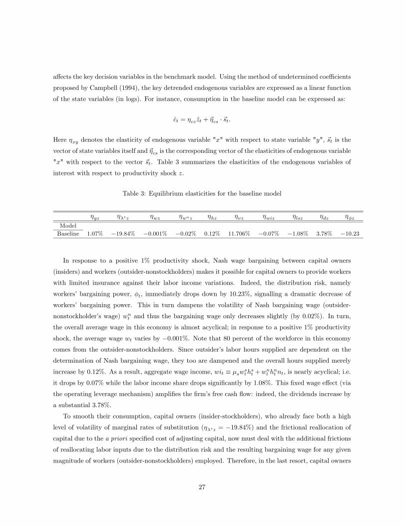
"x" with respect to the vector ~st. Table 3 summarizes the elasticities of the endogenous variables of

interest with respect to productivity shock z.

Table 3: Equilibrium elasticities for the baseline model

�yz ��sz �wz �wnz �hz ��z �wiz �lsz �dz ��zModelBaseline 1.07% �19.84% �0.001% �0.02% 0.12% 11.706% �0.07% �1.08% 3.78% �10.23

In response to a positive 1% productivity shock, Nash wage bargaining between capital owners

(insiders) and workers (outsider-nonstockholders) makes it possible for capital owners to provide workers

with limited insurance against their labor income variations. Indeed, the distribution risk, namely

workers�bargaining power, �t, immediately drops down by 10.23%, signalling a dramatic decrease of

workers� bargaining power. This in turn dampens the volatility of Nash bargaining wage (outsider-

nonstockholder�s wage) wnt and thus the bargaining wage only decreases slightly (by 0.02%). In turn,

the overall average wage in this economy is almost acyclical; in response to a positive 1% productivity

shock, the average wage wt varies by �0.001%. Note that 80 percent of the workforce in this economycomes from the outsider-nonstockholders. Since outsider�s labor hours supplied are dependent on the

determination of Nash bargaining wage, they too are dampened and the overall hours supplied merely

increase by 0.12%. As a result, aggregate wage income, wit � �swsthst +w

nt h

nt nt, is nearly acyclical; i.e.

it drops by 0.07% while the labor income share drops signi�cantly by 1.08%. This �xed wage e¤ect (via

the operating leverage mechanism) ampli�es the �rm�s free cash �ow: indeed, the dividends increase by

a substantial 3.78%.

To smooth their consumption, capital owners (insider-stockholders), who already face both a high

level of volatility of marginal rates of substitution (��sz = �19.84%) and the frictional reallocation ofcapital due to the a priori speci�ed cost of adjusting capital, now must deal with the additional frictions

of reallocating labor inputs due to the distribution risk and the resulting bargaining wage for any given

magnitude of workers (outsider-nonstockholders) employed. Therefore, in the last resort, capital owners

27

Figure 1: Employment �uctuations: baseline model

end up seeking to increase employment in the next period, nt+1, by enormously increasing job vacancy

postings; in other words, expecting trading frictions due to imperfect job matches in the labor market

for outsider-nonstockholders, capital owners (�rms) increase job vacancies by 11.706%. As they build

up the employment level of workers in the following period, market tightness also increases dramatically

while the unemployment decreases persistently (See Figure 1). As capital owners build up the labor

stock of workers, however, wage income gets more risky than output, and, after one year, the rise of

wage income exceeds that of output; in other words, the operating leverage e¤ect or the �xed wage

income e¤ect is completely destroyed after one year. We conclude that our operating leverage channel

is a short-run mechanism for shifting workers�labor income risk on to the capital owners.

In sum, we argue that the short-run operating leverage channel is the key mechanism for resolving

the unemployment puzzle. Distribution risk plays a key role in generating this short-run operating

leverage channel: the countercyclical distribution risk (workers�bargaining power) dampens the resulting

equilibrium bargaining wages signi�cantly, creating the rigid wage income e¤ect.

Aggregate volatilities: Qualitatively, the model respects the basic business cycle stylized facts quite

well: investment volatility exceeds that of output which, in turn, exceeds that of consumption. Aggregate

hours volatility is only slightly less than output, as in the data. As Table 2 shows, however, there

is a downside: the absolute volatilities of consumption and investment depart from their empirical

counterparts. Total consumption has 95 percent of the volatility of output and investment is only

28

one and half times as volatile as output. These results may be laid at the feet of our model�s capital

adjustment costs. As well documented in Jermann (1998), capital adjustment costs make it more costly

to smooth consumption through changing the capital stock, resulting in a lower volatility of investment.

Consumers end up taking more consumption risk (higher volatility of total consumption).

Financial statistics: the equity premium: For the basic return statistics related to the equity

premium �the short rate (or one-period risk free rate), the return on equity, and the premium itself

(all averages) �the model provides a quite reasonable match of theory to data (see Table 4). Return

volatilities are especially close to their empirical counterparts (the Mehra and Prescott (1985) statistics).

As is typical of this style of model, the mean risk free rate is a bit too high and the mean equity return

about one and one-half percentage points too low relative to the period (1889-1978) studied by Mehra

and Prescott (1985). For the expanded period 1871-1993, however, Campbell and Cochrane (1999)

report a U.S. equity premium of 3.9% which is very similar to its model generated counterpart.

Table 4: Financial statistics: the baseline model

Financial StatisticsVariable Meaning Mean Std

Data Model Data ModelRf risk-free bond return 0.80 1.24 5.67 6.48Re equity return 6.98 5.48 16.54 17.71Rp equity premium 6.18 4.28 16.67 17.40

Financial statistics: the term structure: It is well documented that standard RBC models (e.g.,

the indivisible labor model of Hansen (1985)) with persistent technology shocks generate a downward-

sloping average real term structure, as shown in the 4th column of Table 5 (the "RBC model"). In

contrast, the average real term structure generated by the present model is upward sloping with volatility

declining with a longer time to maturity (Benchmark calibration in Table 2). Based on return data for

U.S. traded TIPS, McCullough�s web page reports that the average real term structure for the U.S.

is also upward sloping, a fact con�rmed by Sinha (2010) using an expanded TIPS data set (Table 5).

Using much more extensive U.K. in�ation indexed security returns Sinha (2010) also con�rms an upward

sloping real term structure for that nation as well. Mishkin�s (1990) conclusion that the real and nominal

term structures move together also argues for an upward sloping real term structure. While the present

model does well regarding the replication of this particular term structure shape, and the declining

volatilities, the absolute level of returns and return volatilities remain somewhat excessive vis-a-vis the

data.

The intuitive explanation behind the positive slope is as follows: Although our preference speci�ca-

29

tion does not belong to a class of "generalized expected utility" preferences, the baseline model conveys

the sense that there is strong preference for late resolution of uncertainty among agents in the model

economy: in other words, CRRA = = 3:6 � 1EIS = 1

0:0307 = 25:25. Here the EIS is understood

as the model-implied aggregate EIS, computed as per Appendix 2. When there is a preference for a

late resolution of uncertainty, agents prefer to buy short maturity bonds and roll them over instead of

buying long maturity bonds, which pay o¤ only in a single distant time period. As a result, the demand

for short term bonds is high while the demand for long term bonds is low; consequently, the prices of

short term bonds are high relative to the prices of long term bonds.

The same intuition is found in Binsbergen et al. (2008); in their estimated DSGE model with fully

speci�ed Epstein-Zin preferences, they estimate a low elasticity of intertemporal substitution (around

0.06) from upward-sloping (nominal) yield curve data and macro data. Their estimates also satisfy the

condition that CRRA � 1EIS , which further supports the hypothesis that there is strong preference for

a late resolution of uncertainty.

Table 5: Term structure: the baseline model(i)

US Data Model

Nominal Data McCullogh Data Benchmark (this paper) HansenMaturity Mean Std Mean Std Mean SD Mean SD

4 5.60 2.93 1.06 1.61 1.39 6.32 4.0387 0.318 5.81 2.89 1.39 1.37 1.76 5.72 4.0375 0.2712 5.98 2.82 1.69 1.23 2.10 4.98 4.0370 0.2516 6.11 2.79 1.95 1.15 2.37 4.30 4.0368 0.2320 6.19 2.74 2.16 1.09 2.57 3.72 4.0366 0.22

(i) Maturity in quarters. Nominal data is from Wachter (2006).

McCullogh data is drawn from Piazzesi and Schneider (2006).

Shimer�s Calibration: The baseline model also replicates the observed �uctuations in unemployment

and job vacancies at the business cycle frequencies computed in Shimer (2005). In constructing his

statistics, Shimer chooses a much smoother trend component, corresponding to an HP �lter smoothing

parameter of 105. Accordingly, we do the same for both data and model generated statistics. Since a

� = 10; 000 gives rise in the data to a �y = 2%, the model�s �� must be correspondingly increased to

match this �gure for the model�s detrended output. A choice of �� = :812% accomplishes this goal;

otherwise, all the parameter choices are taken from the benchmark parameter parameterization.

Table 6 replicates the results of this exercise. As would be expected, all volatilities are higher under

this new decomposition. Nevertheless, the match of model statistics to data continues to be very close.

4.2 Attribution of Results

30

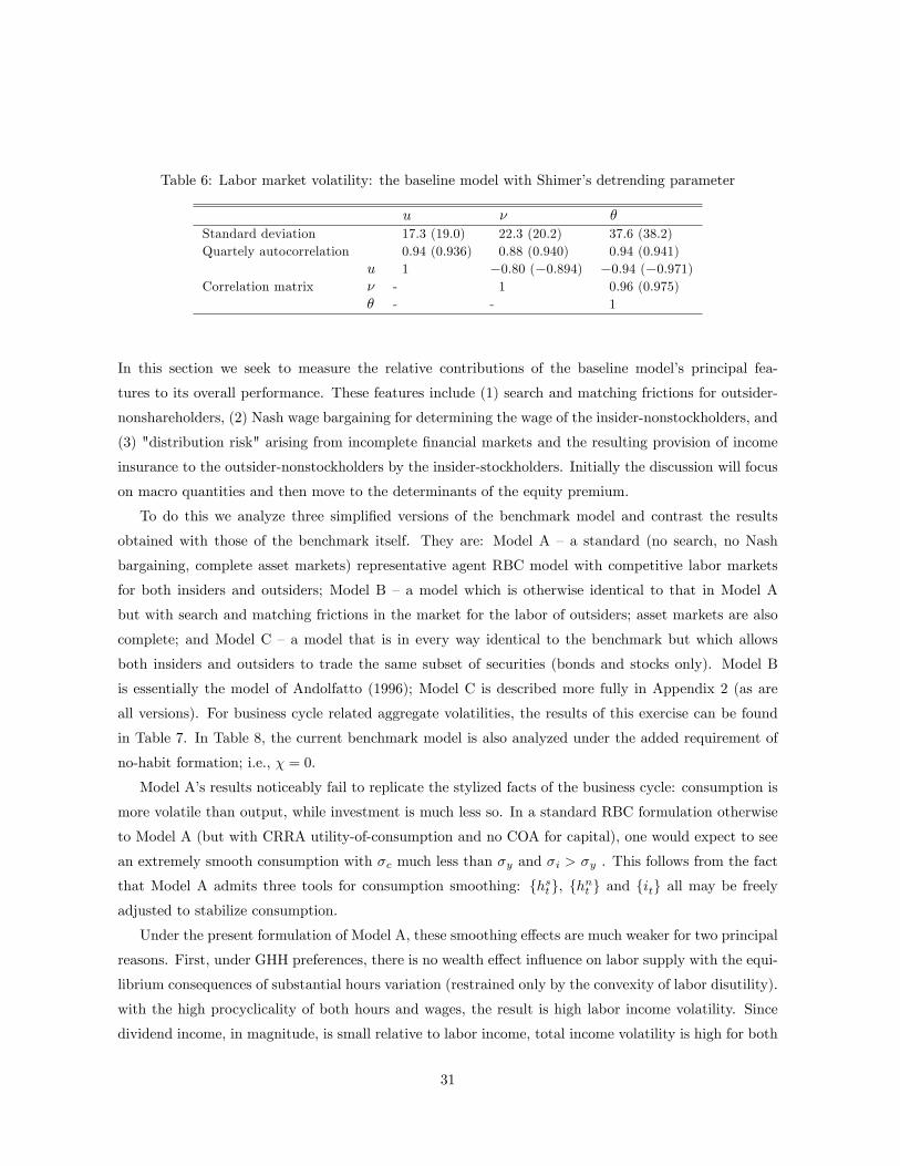
Table 6: Labor market volatility: the baseline model with Shimer�s detrending parameter

u � �Standard deviation 17.3 (19.0) 22.3 (20.2) 37.6 (38.2)Quartely autocorrelation 0.94 (0.936) 0.88 (0.940) 0.94 (0.941)

u 1 �0.80 (�0.894) �0.94 (�0.971)Correlation matrix � - 1 0.96 (0.975)

� - - 1

In this section we seek to measure the relative contributions of the baseline model�s principal fea-

tures to its overall performance. These features include (1) search and matching frictions for outsider-

nonshareholders, (2) Nash wage bargaining for determining the wage of the insider-nonstockholders, and

(3) "distribution risk" arising from incomplete �nancial markets and the resulting provision of income

insurance to the outsider-nonstockholders by the insider-stockholders. Initially the discussion will focus

on macro quantities and then move to the determinants of the equity premium.

To do this we analyze three simpli�ed versions of the benchmark model and contrast the results

obtained with those of the benchmark itself. They are: Model A � a standard (no search, no Nash

bargaining, complete asset markets) representative agent RBC model with competitive labor markets

for both insiders and outsiders; Model B �a model which is otherwise identical to that in Model A

but with search and matching frictions in the market for the labor of outsiders; asset markets are also

complete; and Model C �a model that is in every way identical to the benchmark but which allows

both insiders and outsiders to trade the same subset of securities (bonds and stocks only). Model B

is essentially the model of Andolfatto (1996); Model C is described more fully in Appendix 2 (as are

all versions). For business cycle related aggregate volatilities, the results of this exercise can be found

in Table 7. In Table 8, the current benchmark model is also analyzed under the added requirement of

no-habit formation; i.e., � = 0:

Model A�s results noticeably fail to replicate the stylized facts of the business cycle: consumption is

more volatile than output, while investment is much less so. In a standard RBC formulation otherwise

to Model A (but with CRRA utility-of-consumption and no COA for capital), one would expect to see

an extremely smooth consumption with �c much less than �y and �i > �y . This follows from the fact

that Model A admits three tools for consumption smoothing: fhstg, fhnt g and fitg all may be freelyadjusted to stabilize consumption.

Under the present formulation of Model A, these smoothing e¤ects are much weaker for two principal

reasons. First, under GHH preferences, there is no wealth e¤ect in�uence on labor supply with the equi-

librium consequences of substantial hours variation (restrained only by the convexity of labor disutility).

with the high procyclicality of both hours and wages, the result is high labor income volatility. Since

dividend income, in magnitude, is small relative to labor income, total income volatility is high for both

31

Table 7: Relative aggregate volatilities for a variety of related models

Aggregate Statistics

Data Model A Model B Model C Model 4(baseline)

(a) (b) (c) (a) (b) (c) a) (b) (c) (a) (b) (c) (a) (b) (c)y 1.59 1.59 1.47c 1.23 .77 .83 1.70 1.07 1.00 1.39i 4.87 3.06 .91 1.26 .79 1.00 2.22k

htot .69 .05 .92 1.34hs 1.13 .71 � 1.05hn 1.13 .71 � .56w .70 .44 .68 1.00 .37ws .46 .29 � .42wn .46 .29 � .23n 1.02 .64 .78 � � .90u 11.01 6.92 �.87 � � 10.36v 13.15 8.27 .91 � � 13.42� 21.66 13.62 .90 � � 22.52� � �� .712 .668

Financial Statistics

Data Model A Model B Model C Model 4E[Ret ] 6.98 3.80 5.48�[Ref ] 16.54 2.91 17.71E[Rft ] .80 3.59 1.24�[Rft ] 5.67 .96 6.48E[Rpt ] 6.18 .21 4.28�[Rpt ] 16.67 17.40(i) ( a ) s t a n d a rd d e v ia t io n , ( b ) s .d ./�y , ( c ) c o r r (x; y) f o r a l l a g g r e g a t e s "x"

(ii)Fo r a l l c a s e s = 3:6; � = :99; � = :36; �s = :20; = 1:4; � = :23; � = :5; b=wnhn = :9; � = :08 n = :5; q = :7, e t c . a s a p p l i c a b le .

agent groups. With savings being undertaken exclusively by the �rm under our decentralization scheme,

consumption volatilitly for both agents is high relative to output.24 Second, the COA on capital makes

it expensive for the planner to smooth consumption via investment variation. Discouraged from doing

so he selects a smooth investment series. While high hours volatility would naturally go in tandem with

low wage volatility (as observed), wage variation is conterfactually low.25 Finally, with full employment

at all times, there is no unemployment as vacancy volatility. All in all, Model A can be judged to fail

24Note that for Model A, , , Bn and Bs are the same for both agents. Under complete �nancial markets, there isperfect income insurance and cnt = cst = ct with competitive labor markets and identical utility parameters, wages andthe wage bill are perfectly correlated with output and proportional to one another. With perfect risk sharing, �t � 1; anddisplays no volatility.25This low wage volatility, however, holds promise that GHH preferences will be a signi�cant determinant of any

resolution to Shimer�s puzzle.

32

along the aggregate dimensions, especially those of special interest in the present paper.

The same comment applies to the �nancial dimensions of the model. While consumption volatility

is high on a relative basis, it is still low in an absolute sense with the result that both agents view the

equity and debt securities as pretty much equivalently risky. Accordingly, the premium is a miserable

.21% and all return volatilities are dramatically too low.

Table 8: Robustness: business cycles

�u=�y ��=�y ��=�y �(u; �) �th=�y �h=�y �w=�y ��=�y �(�; y) �(ls; y)

Data 6.92 8.27 13.62 �0.88 0.95 0.43 0.44 � � �0.053*Model

Limited participation modelsBaseline 7.05 9.13 15.32 �0.79 0.91 0.44 0.25 5.38 �0.89 �0.03No habit 5.82 7.57 12.66 �0.78 0.75 0.37 0.20 4.77 �0.95 �0.39

Full participation modelsSH model 0.675 2.58 3.01 �0.55 0.69 0.67 0.45 0 � 0.98AndolfattoHansen � � � � 0.77 0.77 0.28 0 � �.

Table 9: Robustness: �nancial statistics for a variety of models

E[Rft ] �[R

ft ] E[R

et;t+1] �[R

et;t+1] E[R

et;t+1�R

ft ] �[R

et;t+1�R

ft ]

Data 0.80 5.67 6.98 16.54 6.18 16.67Model

Limited participation modelsBaseline 1.24 6.48 5.48 17.71 4.28 17.40Optimized 0.11 5.98 4.96 17.47 4.89 17.00No habit 2.205 2.706 3.82 8.33 1.61 7.77Danthine-Donaldson 2.46 4.05 5.92 22.20 3.46 22.34

Full participation modelsSH model 1.93 5.04 4.65 13.93 2.76 14.44AndolfattoHansen 4.10 0.37 4.11 0.52 0.01 �

To analyze the e¤ect of our distribution risk and the interaction between our distribution risk and

limited asset market participation, we compare our benchmark model with a business cycle model with

search but which allows all to have the full access to the �nancial market, i.e. in which there is no limited

asset market participation, although segmented labor markets are retained. This is Model 3. This search

model is the representative agent (family) model that shares with our baseline model the preference

speci�cation of agents (a hybrid of GHH preference and external habit formation), the presence of

33

two segmented labor markets including search-matching labor market and the capital accumulation

technology with adjustment cost except the limited asset market participation. The model also can

generate a sizable equity premium. Therefore, the model is a good reference point to analyze the e¤ect

of limited asset market participation in our context26 .

The contribution of habit formation to model performance can be inferred from the data presented in

Tables 8 and 9. Comparing the "baseline" and "no habit" lines of Table 8, we see that habit formation

contributes signi�cantly to model volatility, particularly as regards the labor market: unemployment,

tightness, vacancies, and wage volatility all decline with the habit feature, and it alone, is removed.

With the exception of � (`s; y), the correlation structure, however, is not much changed.

This result has its origins in the interaction of the Nash-bargaining wage determination with the

partial income insurance mechanism arising from the asymmetrical security trading opportunities. Under

habit formation, the insider-shareholders display a much-heightened desire to stabilize their marginal

utility of consumption. In response the �rm acts in a manner to stabilize its aggregate wage bill by

reducing the volatility of vacancies, wages, and hours.27 Reduced volatility in employment and labor

market tightness follows as an equilibrium consequence. With both insider-shareholder and outsider-

nonshareholder income volatility reduced, the volatility of the distribution risk measure simultaneously

declines. Accordingly, there is less need for implicit income insurance; the volume of bond trading

declines (not shown) and the share of income to worker nonstockholders increases.

4.3 Relative Model Performance: Comparisons with the Literature

Unemployment volatility puzzle We begin by comparing the results of our benchmark model

with those of two other leading business cycle models with search and matching frictions, namely,

Gertler and Trigari (2005) and Christo¤el and Kuester (2008). We also compare our model with the

existing benchmark business cycle models with search such as Andolfatto (1996) and Merz (1995) and

the standard RBC model of Hansen (1985).

Table 10 shows that our model and the two models with staggered Nash bargaining wage can account

well for the observed volatility in the key labor market variables emphasized by Shimer (2005) and Hall

(2005). In addition, our model and the Christo¤el-Kuester (2008) model capture variations at the

intensive margin as well as at the intensive margin. These latter models account especially well for the

amplitude of the volatilities of the key labor market indicators including unemployment and vacancies.

Nevertheless, Table 10 could reasonably support the assertion that the model of this paper best

replicates the stylized facts of the U.S. labor market; at least as regards the critical volatilities and26 It deserves being mentioned that a direct representation of the baseline model without limited asset market participa-

tion is not trivial; this results from the de�nition of Nash bargaining wage between capitalists and workers, which requiresthat the �rm�s crucial intertemporal decisons be all in accord with the intertemporal marginal rate of substitution of thecapitalists only.27Because of capital costs of adjustments it is more costly to stabilize consumption by allowing more investment volatility.

34

Table 10: Comparison: labor market volatility

�y �u=�y ��=�y ��=�y �n=�y �htotal=�y �h=�y �w=�y �(w; y) �(u; �)

Data 1.59 6.92 8.27 13.62 0.64 0.95 0.43 0.44 0.68 �0.88This paper 1.47 7.05 9.13 15.32 0.61 0.91 0.44 0.25 0.88 �0.79Gertler-Trigari � 5.68 7.28 12.52 0.44 � � 0.48 0.55 �Christo¤el-Kuester 1.91 5.74 7.23 � � 1.09 0.78 0.22 0.09 �Merz 1.07 4.63 6.38 1.67 � � 0.51 � 0.95 �0.15Andolfatto 1.45 0.68* 3.20* 2.64 0.51 0.59 0.22 0.39 0.95 �0.19Hansen 1.76 � � � � 0.77 0.77 0.28 0.87 �Notes: The statistics from Gertler and Trigari (2005) are from their model with the staggeredness � =11/12, i.e 4 quarters.The statistics from Merz (1995) are from her model with �xed search intensity. *numbers in the Andolfatto model are theones reproduced by Costain and Reiter (2008).

correlations. There are exceptions, however; e.g., Christo¤el and Kuester (2008) dominate on the relative

wage volatilitiy dimension, �w�y . On the basis of labor market related quantities, the evidence supports our

assertion that limited asset market participation is an important ingredient for understanding observed

labor market behavior.

Gertler and Trigari (2009) embed the standard Nash bargaining wage contracting into the framework

of (Calvo-type) staggered multiperiod wage contracting while retaining a setting of complete �nancial

markets. Their wage contract ends up taking the form of a �xed wage over an exogenously given horizon.

The Gertler-Trigari (2009) model is quite successful in accounting for the overall volatility in the data

when average wage contract length is assumed to be four quarters (the fourth row of Table 10). The

model, however, is silent about how variations at the intensive margin a¤ects its quantitative validity; in

other words, the model completely abstracts from variable labor hours. As observed in the Andolfatto

(1996) and Merz (1995) models, we cannot exclude the possibility that the output of the Gertler-Trigari

(2009) model is extremely sensitive to variations of labor hours.

Christo¤el and Kuester (2008) incorporate search frictions in the labor market into a New Keynesian

framework characterized by price rigidities in the goods market. Building on the concept of right-to-

manage Nash wage bargaining proposed by Trigari (2006), the Christo¤el-Kuester model can account for

the observed variations of key indicators of labor market activity, including vacancies and unemployment,

as well as the variations at the intensive margin (�fth row of Table 10). To reproduce the empirically

pronounced �uctuations in the level of unemployment over the business cycle, the model must rely on

(i) multiple shocks including productivity shocks, monetary policy shocks, government spending shocks,

and a risk premium shock, (ii) an exogenously speci�ed duration of the wage contract (�ve months) and

(iii) exogenously speci�ed �xed costs of maintaining an existing job which amplify pro�t �uctuations

for any given degree of wage �uctuations. A notable feature of the Christo¤el-Kuester (2008) model is

35

that it requires the same operating leverage channel to give a satisfactory replication of the pronounced

�uctuations of unemployment. Without an exogenous risk premium shock or ad hoc �xed costs of job

maintenance, pro�t �uctuations for any given degree of wage �uctuations are completely destroyed,

i.e. the operating leverage is completely absent. In contrast, our model completely endogenizes the

operating leverage channel. Table 11 summarizes the features of the Gertler and Trigari (2009) and

Christo¤el and Kuester (2008) models as compared to our benchmark formulation.

Table 11: Comparative model features

This paper Gertler-Trigari Christo¤el-Kuester

Productivity shock Yes Yes YesGovernment spending shock No No YesMonetary policy shock No No YesRisk premium shock No (endogenous risk premium) No YesDuration of Nash bargaining wage contract one quarter 3-4 quarters 5 monthsExtensive margin Yes Yes YesIntensive margin Yes No YesModel type RBC model with real rigidites RBC model NK model

From the perspective of model parsimony, Table 11 certainly suggests that the model formulation

of the present paper dominates Christo¤el and Kuester (2008). With respect to hours variation at the

intensive margin, it is quite possible that the addition of this feature will compromise the results in

Gertler and Trigari (2009). Nevertheless, the features of this latter model by which the Nash bargained

wage is renegotiated approximately at annual frequencies is admittedly more realistic than the present

model�s quarterly scenario. Unfortunately, none of the alternative models discussed thus far provides

�nancial statistics. The �nancial performance of the model must thus be judged under a di¤erent set

of benchmarks.

Equity premium puzzle In this section, we begin by comparing the output of our model with that

of several leading macro-asset pricing models proposed in the existing literature; in particular, Boldrin,

Christiano and Fisher (2001), Danthine and Donaldson (2002), Givenen (2003) and Jermann (1998).

To maximize the model�s ability to match stylized �nancial statistics, we now set up a hyperparameter

search slightly di¤erent from the baseline calibration. Assuming that � = 0:9 and � = 0:23, we conduct a

hyperparameter search for the reduced number of free parameters ( , , ��) to match a smaller number

of �nancial statistics of interest. Speci�cally, we choose the free parameters ( , , ��) to match three

empirical targets: (i) a risk-free rate volatility (iii) the mean risk-free rate and (iv) the equity premium.

Practically, we restrict our hyperparameter search to a grid of values for �� 2 [0:0037; 0:00712]; 2 [1; 2]and 2 [1; 7]. We then minimize a weighted quadratic criterion function written in the deviation from

36

each empirical target with common weight of 1 with the exception of a weight of 10 for risk-free rate

volatility. The minimum is achieved for �� = 0:0052; = 1:26 and = 4:5. The coe¢ cient of relative

risk aversion jumps to 4.5 from the benchmark case of 3.6; = 1:26 implies that the Frisch elasticity of

labor supply in this economy is 11:26�1 = 3:846 which is similar to the Imai-Kean estimate of 3.8. Our

value of the innovation standard deviation, ��, is 0.52%, which is even smaller than the value of our

benchmark model, 0.6%.

Tables 12 and 13 display the statistics from the simulated models along with their empirical coun-

terparts from US data. The model optimized by the above method of hyperparameter search (hereafter

the "optimized model") generates an equity premium of 4.89%, which, not surprisingly, is higher than

the baseline model. The standard deviation of excess returns is 17.00%, which is broadly consistent

with the empirical magnitude of the standard deviation of excess returns found in the US data� - the

standard deviation of excess returns is estimated to be 16.67%. The volatility of the average risk-free

rate is 5.98%, which achieves a satisfactory replication of its empirical counterpart, 5.67%. The average

risk-free rate, however, is 0.11%, which is too low vis-a-vis its empirical target of 0.80% in the US data.

Table 12: Model comparision: �nancial statistics

E[Rft ] �[R

ft ] E[R

et;t+1] �[R

et;t+1] E[R

et;t+1�R

ft ] �[R

et;t+1�R

ft ]

Data .80 5.67 6.98 16.54 6.18 16.67ModelBaseline 1.24 6.48 5.48 17.71 4.28 17.40Optimized (Shimer�s parameters) 0.11 5.98 4.96 17.47 4.89 17.00Danthine-Donaldson 2.46 4.05 5.92 22.20 3.46 22.34Guvenen (2003) 1.98 5.73 5.30 14.10 3.32 14.70Boldrin-Christiano-Fisher 1.20 24.6 7.83 18.4 6.63 �Jermann 0.82 11.64 7.00 19.86 6.18 �Hansen 4.05 0.46 4.04 0.48 0.01 .0013

Most �nance-cum-production models require that the capital owner display a strong desire to smooth

his consumption intertemporally while simultaneously acting in a context that makes it di¢ cult to

reallocate labor or capital to that same end. The frictions attendant to reallocating labor or capital

are key to generating a high equity premium. Essentially, they substitute for some form of market

incompleteness: in either case, agents are prevented from smoothing their consumption across states

and dates. Both our baseline model and its optimized cousin are in this tradition: capital owners,

who already face a high level of MRS volatility and the costly reallocation of capital due to the capital

adjustment costs, now must also deal with the additional friction of reallocating labor inputs.

A distinguishing feature of our mechanism is that the model still can achieve a satisfactory replication

of the stylized �nancial statistics despite allowing for variations at both the intensive and the extensive

37

Table 13: Model comparison: aggregate volatilities

�y �c=�y �i=�y �htot=�y �h=�y �(c; y) �(i; y) �(th; y) �(h; y)

Data 1.59 0.77 3.09 0.95 0.43 0.83 0.91 0.92 0.62ModelBaseline 1.47 0.95 1.51 0.91 0.44 0.94 0.86 0.90 0.94Optimized 1.28 0.96 1.73 1.02 0.23 0.89 0.82 0.88 0.86Danthine-Donaldson 1.77 0.82 1.72 � � 0.96 0.93 � �Guvenen (2003) 2.40 0.96 1.13 � � � � � �Boldrin-Christiano-Fisher 1.97 0.69 1.67 0.51 0.51 0.95 0.97 0.86 0.86Jermann 1.76 0.49 2.64 � � � � � �Hansen 1.76 0.29 3.24 0.77 0.77 0.87 0.99 0.98 0.98

margins. Most macro-asset-pricing models assume that the labor supply is inelastic or, when endogenous

labor supply choice is incorporated, the models usually display low volatility of total hours worked, which

comes close to the observed volatility of hours per worker rather than that of total hours. Therefore,

variations at the extensive margin are frequently ignored in this class of the models.

The essence of our mechanism for generating a substantial equity premium, partial risk-sharing

manifest as endogenous distribution risk, generates less risky shares of income going to labor in the

short run: wage bills vary less than output, falling proportionately less in recessions and increasing less

during expansions relative to an uninsured scenario. As a result, the risk in the �rm�s free cash �ow

and derived dividends increases substantially due to the semi-�xed wage bill.

As in the previous section, additional insight as to the source of the equity premium can be obtained

by examining the model�s impulse response functions. In what follows, we emphasize that the operating

leverage e¤ect is the key to generating a high equity premium. Table 14 summarizes the elasticities

of the endogenous variables of interest with respect to a productivity shock z. As reference points, we

summarize the elasticities of the endogenous variables from the benchmark model and the standard

RBC model of Hansen (1985).

Table 14: Comparative elasticities

�yz ��sz �wz �wnz �hz ��z �wiz �lsz �dz ��zModelBaseline 1.07% �19.84% �0.001% �0.02% 0.12% 11.706% �0.07% �1.08% 3.78% �10.23%Optimized 0.96% �27.05% �0.05% �0.07% �0.05% 17.05% �0.34% �1.21% 0.33% �20.07%Hansen 1.94% 0.47% � 1.37% � 1.94% � �8.62% �

Figure 2 presents the impulse response functions from the optimized model. As in the benchmark

38

Figure 2: Impulse response of macroaggregates to a one time positive productivity disturbance: opti-mized model

model, the optimized version highlights the signi�cance of the operating leverage e¤ect. In response to

a positive 1% productivity shock, the optimized model displays a 20.07% decrease of the distribution

risk �t sensitivity to a positive productivity shock, ��z, thereby dampening wage income sensitivity by

0.34%. Furthermore, as Figure 2 clearly indicates, this operating leverage e¤ect is more persistent in

the "optimized model" than in the benchmark case: after approximately one and half years, the wage

income is more a¤ected than output (the increase in wage income exceeds the increase in output).

Intuitively, high-productivity shocks coincide with the situations where the bargaining power of

capitalists is high and the bargaining power of workers is low. As a result, the high residual payment

to capitalists due to the high-productivity realization is further magni�ed by the decrease of the labor

income share. Accordingly, the �rm�s free cash �ow and derived dividends increase during the boom.

Conversely, low productivity shocks reduce further the already low residual payment to capitalists. We

have argued that the persistent procyclicality of the residual payments to capitalists can generate a

sizable equity premium.

Let us summarize these remarks. There are several main channels to achieving a high equity premium

cited in the existing literature.28 First, there is the operating leverage channel with idiosyncratic distri-

bution risk, as advocated by Danthine and Donaldson (2002) and the present model, which postulates

28As noted earlier, these leading macro-asset-pricing models abstract from the wedge between variations at the intensivemargin and at the extensive margin. In other words, variations at the extensive margin are ignored in this class of themodels.

39

that capital owners e¤ectively provide nonshareholder-workers with insurance against the latter group�s

income variation as a byproduct of security trading. This risk-sharing mechanism, ceteris paribus, cre-

ates a high level of volatility of shareholder consumption. This occurs in a setting where the shareholders

can themselves mitigate high consumption volatility via the posting of vacancies and the management

of the capital stock. Yet, they are discouraged from doing so by high adjustment costs at each margin.

As a result, the risk properties of the residual payments to �rm owners, in equilibrium, are magni�ed

and a substantial risk premium is achieved.

This channel originates from limited participation in the stock market and heterogeneity in the

elasticity of intertemporal substitution in consumption. Insider-shareholders participate in both stock

and bond markets while more risk-averse outsider-nonshareholders trade only bonds. Since bond trading

is their only mechanism for consumption smoothing, nonshareholders bid up bond prices, resulting in a

low risk-free rate. In equilibrium, insider-shareholders end up insuring non-shareholders by increasing

their own debt holdings exactly when a low-productivity realization reduces both agents�income. As

such, bond market events serve to smooth the consumption of non-stockholders and amplify the volatility

of shareholder consumption. As a result, stockholders demand a large premium for holding aggregate

risk (Guvenen (2003)).

Second, the magnitude of the equity premium is enhanced by the strong consumption smoothing

motives of the insider-shareholders arising from habit formation preferences. This feature has nothing

to do with outsider-nonshareholder income insurance, but reinforces the e¤ects of it to increase further

the volatility of the insider-shareholder�s marginal rate of substitution.

Third, given the strong insider-shareholder motives for consumption smoothing arising from channels

one and two above, these same agents are discouraged from doing so by the costs of adjusting capital

and labor (the latter in the form of the cost of adjusting vacancies).

5 Concluding Remarks

In response to the unsatisfying empirical performance of the conventional model of unemployment

dynamics due to Mortensen and Pissarides, a recent body of studies (Merz (1993), Andolfatto (1996) and

Gertler and Trigari (2009)) has emphasized the importance of the degree of wage rigidity in accounting

for observed volatility in variables characterizing labor market activity over the business cycle. In this

paper, we extend the Mortensen and Pissarides model with Nash wage bargaining to an environment

where the asset market is incomplete and perfect risk-sharing between capital owners and workers

cannot be guaranteed. We develop period-by-period Nash wage bargaining between capitalists and

workers in a macro model with two key features: limited participation in the stock market and labor-

force heterogeneity (permanently employed insiders and outsiders subject to employment variation).

40

What emerges from these considerations is a short-run operating leverage e¤ect which substantively

assists in overcoming the unemployment volatility puzzle emphasized by Shimer (2005) and Hall (2005).

Speci�cally, the operating leverage e¤ect may be interpreted as serving the role of an endogenous Nash

bargaining power shock perfectly analogous to the exogenous Nash bargaining power shock proposed

by Shimer (2005). As such, our model can be viewed as an attempt to provide microfoundation for

Shimer�s proposed Nash bargaining power shock. This operating leverage e¤ect simultaneously provides

a mechanism for generating a sizable equity premium. In summary, a reasonable calibration of the

resulting model, which successfully replicates the basic �nancial statistics, also accounts well for not

only for aggregate �uctuations in unemployment and vacancies and their negative correlation, but also

for the observed wedge between variations at the intensive margin (hours per worker) and at the extensive

margin (total hours) over the business cycle. In contrast to existing leading macro-asset-pricing models,

the model is unique in the sense that without compromising the overall performance on the �nancial

front, it can pretty much fully reproduce the stylized business cycle facts of the labor market activity.

Many years of research on the properties of DSGE models suggest that it is the allocation of risks

across the various economic participants that determines the ability of models to explain jointly the

�nancial stylized facts and the basic properties of macro aggregates. With respect to the latter, the

replication of labor market related statistics has historically proven to be generally the most challenging.

Clearly, the assignment of risks cannot be separate from the �nancial market structure confronting a

model�s economic agents. It is in this spirit that we have elected to impose upon a DSGE model with

well understood labor market features (search and matching cum Nash wage bargaining) an empirically

realistic incomplete �nancial market structure.

41

ReferencesAbel, A. B. 1990. "Asset Prices under Habit Formation and Catching Up with the Joneses," American

Economic Review 80:38-42.

Andolfatto, D.1996. "Business Cycles and Labor Market Search," American Economic Review

86:112-132.

Barro, R. J. 1977. "Long-term Contracting, Sticky Prices, and Monetary Policy," Journal of Monetary

Economics 3:305-316.

Binsbergen, J. H. v., J. Fernandez-Villaverde, R. S. J. Koijen, and J. F. Rubio-Ramirez. 2008.

"Working with Epstein-Zin Preferences: Computation and Likelihood Estimation of DSGE Models

with Recursive Preferences," mimeo.

Boldrin, M., L. J. Christiano, and J. D. M. Fisher. 2001. "Habit Persistence, Asset Returns, and the

Business Cycle," American Economic Review 91:149-166.

Boldrin, M., and M. Horvath. 1995. "Labor Contracts and Business Cycles," Journal of Political

Economy 103:972-1004.

Campbell, J. Y. 1994. "Inspecting the Mechanism: an Analytical Approach to the Stochastic Growth

Model," Journal of Monetary Economics 33:463-506.

Campbell, J.Y., and J. Cochrane. 1999. "By Force of Habit: A Consjmption Based Explanation of

Aggregate Stock market Behavior," Journal of Political Economy 107: 205-251.

Chéron, A., and F. Langot. 2004. "Labor Market Search and Real Business Cycles: Rconciling Nash

Bargaining with Real Wage Dynamics," Review of Economic Dynamics 7:476-493.

Christiano, L. J., C. Ilut, R. Motto, and M. Rostagno. 2007. "Monetary Policy and Stock Market

Boom-Bust Cycles," mimeo.

Christo¤el, K., and K. Kuester. 2008. "Resuscitating the Wage Channel in Models with

Unemployment Fluctuations," Journal of Monetary Economics 55:865-887.

Costain, J., and M. Reiter. 2008. "Business Cycles, Unemployment Insurance, and the Calibration of

Matching Models," Journal of Economic Dynamics and Control 32:1120-1155.

Cooley, T. F., and E. C. Prescott. 1995. "Economic Growth and Business Cycles," in T. F. Cooley

ed., Frontiers of Business Cycle Research, Princeton: Princeton University Press, pp. 1-38.

Cooley, T. F., and V. Quadrini. 1999. "A Neoclassical Model of the Phillips Relation," Journal of

Monetary Economics 44:165-193.

Cooley, T. F., and V. Quadrini. 2004. "Optimal Monetary Policy in a Phillips-Curve World," Journal

of Economic Theory 118:174-208.

Danthine, J. P., and J. B. Donaldson. 2002. "Labor Relations and Asset Returns," Review of

Economic Studies 69:41-64.

Danthine, J. P., J. B. Donaldson, and R. Mehra. 1992. "The Equity Premium and the Allocation of

Labor Income Risk," Journal of Economic Dynamics and Control 16:509-532.

42

Danthine, J. P., J. B. Donaldson, and P. Siconol�. 2008. "Distribution Risk and Equity Premium," in

R. Mehra ed., Handbook of the Equity Risk Premium, Amsterdam: North-Holland, pp. 415-466.

Donaldson, J. B., and R. Mehra. 1984. "Comparative Dynamics of an Equilibrium Intertemporal

Asset Pricing Model," Review of Economic Studies 69:491-508.

Donaldson, J. B., T. Johnsen, and R. Mehra. 1990. "On the Term Structure of Interest Rates,"

Journal of Economic Dynamics and Control 14:571-596.

Davis, S., J. Haltiwanger, and S. Schuh. 1996. Job Creation and Destruction, Cambridge: MIT Press.

Farmer, R. 2004. "Shooting the Auctioneer," mimeo.

Ferson, W. E., and G. M. Constantinides. 1991. "Habit Persistence and Durability in Aggregate

Consumption," Journal of Financial Economics 29:199-240.

Gallmeyer, M., B. Holli�eld, F. Palomino, and S. Zin. 2008. "Term Premium Dynamics and the

Taylor Rule," mimeo.

Gertler, M., and A. Trigari. 2009. "Unemployment Fluctuations with Staggered Nash Wage

Bargaining," Journal of Political Economy 117: 38-86.

Greenwood, J., Z. Hercowitz, and G. Hu¤man. 1988. "Investment Capacity Utilization and the

Business Cycle," American Economic Review 78:402-417.

Guvenen, F. 2003. "A Parsimonious Macroeconomic Model for Asset Pricing: Habit Formation or

Cross-sectional Heterogeneity?" mimeo.

Guvenen, F. 2006. "Reconciling Con�icting Evidence on the Elasticity of Intertemporal Substitution:

A Macroeconomic Perspective," Journal of Monetary Economics 53:1451-1472.

Guvenen, F. 2009. "A Parsimonious Model for Asset Pricing," Econometrica 77:1711-1750.

Hall, R. E. 1988. "Intertemporal Substitution in Consumption," Journal of Political Economy

96:339-357.

Hall, R. E. 2005. "Employment Fluctuations with Equilibrium Wage Stickiness," American Economic

Review 95: 50-65.

Hagedorn, M., and I. Manovskii. 2008. "The Cyclical Behavior of Equilibrium Unemployment and

Vacancies Revisited," American Economic Review 98:1692�1706.

Hansen, G. D. 1985. "Indivisible Labor and The Business Cycle," Journal of Monetary Economics

16:309-327.

Hornstein, A., and H. Uhlig. 2000. "What is the Real Story for Interest Rate Volatility?" German

Economic Review 1:43-67.

Hornstein, A., P. Krusell, and G. Violante. 2005. "Unemployment and Vacancy Fluctuations in the

Matching Model: Inspecting the Mechanism," Federal Reserve Bank of Richmond Economic Quarterly

91:19-51.

Imai, S., and M. P. Keane. 2004. "Intertemporal Labor Supply and Human Capital Accumulation,"

International Economic Review 45:601-641.

43

Jaimovich, N., and S. Rebelo. 2009. "Can News About the Future Drive the Business Cycle?"

American Economic Review 99:1097-1118.

Jermann, U. 1998. "Asset Pricing in Production Economies," Journal of Monetary Economics

41:257-275.

Kim, H. 2008a. "Equity Premium and Search in the Labor Market," mimeo

Kim, H. 2008b. "Insider-Oursider Labor Relation, Asset Returns and the Business Cycle," mimeo

Kim, H. 2008c. "Resuscitating Habit Formation: The Case of Staggered Nash Bargaining Wage,"

mimeo

Krusell, P., T. Mukoyama, and A. Sahin. 2007. "Labor-Market Matching with Precautionary Savings

and Aggregate Fluctuations," mimeo.

Kydland, F. E. 1984. "Labor-Force Heterogeneity and the Business Cycle," Carnegie-Rochester

Conference Series on Public Policy 21:173-208.

Kydland, F. E. and E. C. Prescott. 1982. "Time to Build and Aggregate Fluctuations," Econometrica

50:1345-1370.

Lettau, M. 2003. "Inspecting the Mechanism: The Determination of Asset Prices in the Real Business

Cycle Model," Economic Journal 113:550-575.

Lettau, M., and H. Uhlig. 2002. "Can Habit Formation be Reconciled with Business Cycle Facts?"

Review of Economic Dynamics 3:79-99.

Lucas, R. E.,Jr. 1978a. "Asset Prices in an Exchange Economy," Econometrica 46:1429-1445.

Lucas, R. E.,Jr. 1978b. "On the Size Distribution of Business Firms," Bell Journal of Economics

9:508-523.

McCurdy, 1981.

Mankiw, G., and S. Zeldes. 1991. "The Consumption of Stockholders and Non-Stockholders," Journal

of Financial Economics 29:97-112.

Mehra, R., and E. C. Prescott. 1985. "The Equity Premium: A Puzzle," Journal of Monetary

Economics 22:145-161.

Menzio, G. 2005. "High-Frequency Wage Rigidity," mimeo.

Merz, M. 1995. "Search in the Labor Market and the Real Business Cycle," Journal of Monetary

Economics 36:269-300.

Merz, M., and E. Yashiv. 2007. "Labor and the Market Value of the Firm", American Economic

Review 97:1419-1431.

Mishkin, F. 1990. "What does the Term Structure Tell Us about Future In�ation?," Journal of

Monetary Economics 25:77-95.

Mortensen, D. 1992. "The Cyclical Behavior of Job Creation and Job Destruction," Working paper,

Northwestern University.

Nash, J. F. 1950. "The Bargaining Problem," Econometrica 46:587-594.

44

Petronglo, B., and C. A. Pissarides. 2001. "Looking into the Blackbox: A Survey of the Matching

Function," Journal of Economic Literature 2001:390-431.

Piazzesi, M., and M. Schneider. 2006. "Equilibrium Yield Curves," NBER Macroeconomics Annual :

389-442.

Pissarides, C. 1988. "The Search Equilibrium Approach to Fluctuations in Employment," American

Economic Review 78:363-368.

Pissarides, C. 1990. Equilibrium Unemployment Theory, Oxford: Basil Blackwell.

Poterba, J. 2000. "Stock Market Wealth and Consumption," Journal of Economic Perspectives

14:99-118.

Rogerson, R., and R. Wright. 1988. "Involuntary Unemployment in Economies with E¢ cient Risk

Sharing," Journal of Monetary Economics 22:501-515.

Rosen, S., 1982. "Authority, Control, and the Distribution of Earnings," Bell Journal of Economics

13:311-323.

Roth, Alvin E., and Uriel G. Rothblum. 1982. "Risk Aversion and Nash�s Solution for Bargaining

Games with Risky Outcomes," Econometrica 50:639-647.

Rouwenhorst, G. 1995. "Asset Pricing Implications of Equilibrium Business Cycle Models," in T. F.

Cooley, ed., Frontiers of Business Cycle Research, Princeton: Princeton University Press, pp. 294-330.

Shimer, R. 2005. "The Cyclical Behavior of Equilibrium Unemployment, Vacancies, and Wages:

Evidence and Theory," American Economic Review 95:25-49.

Sinha, A. 2010. "Learning and the Yield Curve," mimeo, Columbia University.

Smets, F., and R. Wouters. 2003. "An Estimated Dynamic Stochastic General Equilibrium Model of

the Euro Area," Journal of European Economic Association, 1:1123-1175.

Sveen, T., and L. Weinke. 2008. "New Keynesian Perspectives on Labor Market Dynamics," Journal

of Monetary Economics 55:921-930.

Trigari, A. 2004. "Labor Market Search, Wage Bargaining and In�ation Dynamics,"

Uhlig, H. 1999. "A Toolkit for Analysing Nonlinear Dynamic Stochastic Models Easily," in Marimon,

R., and A. Scott, eds., Computational Methods for the Study of Dynamic Economies, Oxford and New

York: Oxford University Press, pp. 30-61.

Uhlig, H. 2006. "Macroeconomics and Asset Markets: Some Mutual Implications," mimeo.

Uhlig, H. 2007. "Explaining Asset Prices with External Habits and Wage Rigidities in a DSGE

Model," American Economic Review 97:239-243.

Wachter, J. A. 2006. "A Consumption-based Model of the Term Structure of Interest Rates," Journal

of Financial Economics 79:365-399.

Wei, Min. 2005. "Human Capital, Business Cycles and Asset Pricing," mimeo, Graduate School of

Business, Columbia University.

45

Appendix 1: Model Solution: Asset Pricing

Asset Pricing Let 1+Rt+1 be the gross return on an asset held from period t to period t+1. If the

price and the cash �ow of the asset in period t are denoted by Pt and Ft, respectively, then

1 +Rt+1 =Pt+1 + Ft+1

Pt: (30)

The Arrow-Lucas-Rubinstein asset pricing equation requires that any asset with (30) must satisfy

1 = Et[��t+1�t

(1 +Rt+1)]: (31)

Equivalently, we can rewrite (31) as follows:

0 = log � + logEt[exp(�t+1 � �t + rt+1)] (32)

where �t is the log-deviation of marginal utility of consumption from its steady state value and rt+1 �log(1 + Rt+1). Assuming that �t+1 and 1 + Rt+1 are jointly lognormally distributed and using the

standard formula for the expectation of lognormally distributed variables, equation (32) can be written

as:

0 = log � + Et[�t+1 � �t] + Et[rt+1] +1

2[�2�t + �

2rt + 2��rt��t�rt] (33)

where �2�t � V art[�t+1 � �t] = Et[(�t+1 �Et�t+1)2], �2rt � V art[rt+1] = Et[(rt+1 �Etrt+1)2], and ��rtis the conditional correlation, i.e. ��rt��t�rt � Covt[(�t+1 � �t); rt+1].

Risk-free Rate A risk-free asset (one quarter real bond) with the risk-free rate rft � log(1+Rft ) can

be priced in much simpler way. Since �2rt = Et[(rft+1 � Etr

ft+1)

2] = 0, we have

rft = � log � � Et[�t+1 � �t]�1

2�2�t: (34)

Then the simple risk-free rate is given by

1 +Rft = exp rft :

The unconditional moments of the simple risk-free rate can be calculated using the log-normal formula

for the unconditional expectation:

E[1 +Rft ] = exp(E[rft ] +1

2V ar[rft ])

V ar[Rft ] = V ar[1 +Rft ] = exp(2E[rft ] + 2V ar[r

ft ])� exp(2E[r

ft ] + V ar[r

ft ]):

46

The unconditional moments of rft are given by

E[rft ] = � log � � 12V ar[�t+1 � Et�t+1]

V ar[rft;n] = V ar[Et[�t+1 � �t]]:

Term Structure For the calculation of the conditional term structure fRft;ng, we can apply the samelog-linear and log-normal framework as the risk-free rate case. Note that the conditional term structure

fRft;ng can be represented by

1 +Rft;n = [�nEt[

�t+n�t

]]�1=n:

Denote the quarterly continuously-compounded yield of a n-period real bond by rft;n � log 1 + Rft;n.

Again using the standard formula for the expectation of lognormally distributed variables, we have

rft;n = � 1nlog[�nEt[

�t+n�t

]]

= � log � � 1

nlogEt[exp(�t+n � �t)]

= � log � � 1

n[Et[�t+n � �t] +

1

2�2�t]:

The simple bond yield is given by

1 +Rft;n = exp rft;n:

The unconditional moments of the simple bond yield can be calculated using the log-normal formula for

the unconditional expectation:

E[1 +Rft;n] = exp(E[rft;n] +1

2V ar[rft;n])

V ar[Rft;n] = V ar[1 +Rft;n] = exp(2E[rft;n] + 2V ar[r

ft;n])� exp(2E[r

ft;n] + V ar[r

ft;n]):

The unconditional moments of rft;n are given by

E[rft;n] = � log � � 1

2nV ar[�t+n � Et�t+n]

V ar[rft;n] =1

n2V ar[Et[�t+n � �t]]:

Equity To calculate the equity returns, we adopt a slightly di¤erent strategy. The Arrow-Lucas-

Rubinstein asset pricing equation tells us that the period t equity price pet must equal the present value

47

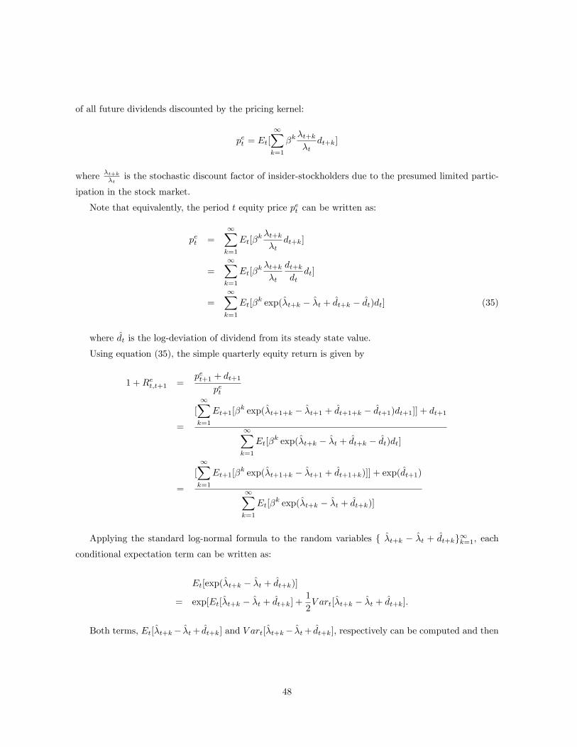
of all future dividends discounted by the pricing kernel:

pet = Et[1Xk=1

�k�t+k�t

dt+k]

where �t+k�t

is the stochastic discount factor of insider-stockholders due to the presumed limited partic-

ipation in the stock market.

Note that equivalently, the period t equity price pet can be written as:

pet =1Xk=1

Et[�k �t+k�t

dt+k]

=1Xk=1

Et[�k �t+k�t

dt+kdt

dt]

=1Xk=1

Et[�k exp(�t+k � �t + dt+k � dt)dt] (35)

where dt is the log-deviation of dividend from its steady state value.

Using equation (35), the simple quarterly equity return is given by

1 +Ret;t+1 =pet+1 + dt+1

pet

=

[1Xk=1

Et+1[�k exp(�t+1+k � �t+1 + dt+1+k � dt+1)dt+1]] + dt+1

1Xk=1

Et[�k exp(�t+k � �t + dt+k � dt)dt]

=

[1Xk=1

Et+1[�k exp(�t+1+k � �t+1 + dt+1+k)]] + exp(dt+1)

1Xk=1

Et[�k exp(�t+k � �t + dt+k)]

Applying the standard log-normal formula to the random variables f �t+k � �t + dt+kg1k=1, eachconditional expectation term can be written as:

Et[exp(�t+k � �t + dt+k)]

= exp[Et[�t+k � �t + dt+k] +1

2V art[�t+k � �t + dt+k]:

Both terms, Et[�t+k� �t+ dt+k] and V art[�t+k� �t+ dt+k], respectively can be computed and then

48

we approximate 1 +Ret;t+1 by

[nXk=1

Et+1[�k exp(�t+1+k � �t+1 + dt+1+k)]] + exp(dt+1)

nXk=1

Et[�k exp(�t+k � �t + dt+k)]

for su¢ ciently large number n.

Appendix 2: A Further Check on Model Legitimacy: Elasticity of In-tertemporal Substitution

To see how the elasticity of intertemporal substitution (EIS) is identi�ed in our preference speci�ca-

tions, �rst note that the equations (7) and (14) can be rewritten as

1

1 +Rft= �E(

�st+1�st

j t) (36)

1

1 +Rft= �E(

�nt+1�nt

j t) (37)

where �st = uc(cs(t); h

s(t)), �nt = vc(c

n(t); hn(t)) and 1

1+Rft= pft .

The period utility function of the representative insider-stockholder is postulated as

u(cst �Xt �H(hst )) =(cst �Xt �H(hst ))1� s � 1

1� s

while the preference of the representative outsider-nonstockholder is postulated as

v(cnt � L(hnt )) =(cnt � L(hnt ))1� n � 1

1� n:

Here s and n are the insider-stockholder�s coe¢ cient of risk aversion and the outsider-nonstockholder�s

coe¢ cient of risk aversion, respectively; Xt is the exogenous habit stock, evolving according to

Xt = �Xt�1 + (1� �)�cst�1

where cst�1 denotes the aggregate average level of the insider-stockholder group�s consumption last

period, � is the habit parameter of the insider-stockholder group and � = 0.

Under the above speci�cations of the each agent�s preference, we log-linearize and rearrange the

equations (36) and (37) in order to obtain the each agent�s EIS (the bar "�" represents the steady state

49

value of variables):

1

s

[�cs(1� �)�H(�hs)]�cs

rft = Et[logcst+1cst

+ [remainder terms]] (38)

1

n

[�cn � �nL(�hn)]�cn

rft = Et[logcnt+1cnt

+ [remainder terms]]: (39)

From the equations (38) and (39), we identify the insider-stockholder�s EIS with

1

s

[�cs(1� �)�H(�hs)]�cs

while the outsider-nonstockholder�s EIS can be identi�ed with

1

n

[�cn � �nL(�hn)]�cn

:

Note also that

logct+1ct

= log(1 +�s(c

st+1 � cst ) + (cnt+1 � cnt )

ct) (40)

� �s(cst+1 � cst )

ct+(cnt+1 � cnt )

ct

� �s logcst+1cst

� cst

ct+ log

cnt+1cnt

� cnt

ct.

Therefore, taking the expectation operator Et in (40) and using the equations (38) and (39), we derive

the formula:

Et[logcst+1cst

+ [remainder terms]]

= [�s1

s

[�cs(1� �)�H(�hs)]�cs

Etcstct+1

n

[�cn � �nL(�hn)]�cn

Etcntct]rft :

We identify the aggregate EIS with

�s1

s

[�cs(1� �)�H(�hs)]�cs

Etcstct+1

n

[�cn � �nL(�hn)]�cn

Etcntct:

Abstracting from uncertainty our identi�ed EIS is reduced to

�s1

s

[�cs(1� �)�H(�hs)]�c

+1

n

[�cn � �nL(�hn)]�c

(41)

which must be the true value of the aggregate EIS in our economy when estimated from the generated

data. Under our benchmark calibration, the aggregate EIS is predicted to be close to zero (0.0307).

50

This predicted number is consistent with Hall�s �ndings: consumption growth is completely insensitive

to changes in interest rates and thus EIS is close to zero. It is also consistent with the conclusion

found in Binsbergen et al. (2008); in their estimated DSGE model, they �nd that a low elasticity of

intertemporal substitution (around 0.06) is estimated from upward-sloping (nominal) yield curve data

and macro data.

Appendix 3: Background Models to Table 71. Model A: A standard RBC model with competitive wage determination for both insiders and

outsiders (no search and matching), and complete �nancial markets.

The notation and all functional forms (i.e., utility functions, the production function) coincide with

those of Section 2 with the sole exception that there is no habit formation stock (Xt � 0) in the

insider-stockholder�s utility representation. Because of the competitive factor markets and complete

asset markets the competitive equilibrium allocation can be obtained by solving the associated Pareto

problem:

maxfcnt ;cst ;hst ;hnt ;itg

E

1Xt=0

�t [�su (cst �H (hst )) + v (cnt � L (hnt ))]

!

s.t. �scst + c

nt + it = f (kt; �sh

st ; h

nt ) ezt

kt+1 = (1� �) kt +G�itkt

�kt; k0 = kss

log ezt+1 = � log zt +e�t+1:In Table 7 we list the statistical summary of this model�s output under "Model 1."

The dividend is de�ned by:

dt = yt � it � �swsthst � wnt hnt � rf�k.

2. Model B: This model is identical to the one described above, but with search and matching in

the labor market for outsider-nonstockholders. A Pareto formulation may also be analyzed:

maxfcst ;cnt ;hst ;hnt ;vtg

E

1Xt=0

�t [�su (cst �H (hst )) + v (cnt � L (hnt )nt � (1� nt)L (0))]

!

s.t. �scst + c

nt +

K2(mt)

2

nt+ it = f (kt; �sh

st ; nth

nt ) ezt

nt+1 = (1� �)nt +mt

mt = �mv�t (1� nt)

1��

kt+1 = (1� �) kt +G�ntkt

�kt

log ezt+1 = � log ezt +e�t+1:In Table 7, the statistical summary of this model�s output is found under the heading "Model 2."

51

The dividend is de�ned by:

dt = yt � it ��K2

� m2t

nt� �shstwst � hnt wnt � r

ft �k

Model B is very similar to that of Andolfatto (1996).

3. Model C: As noted in the main text, this model considers a representative agent (family) that

shares with the baseline model the preference speci�cation of agents (a hybrid of GHH preference and

external habit formation). There are two segmented labor markets including a search-matching labor

market and a capital accumulation technology with adjustment cost. These elements are shared with

Models A and B. Financial markets are not strictly complete but all agents trade the same two securities:

there is no restricted participation.

C.1 The shareholder-worker�s problem is essentially identical to that detailed in Section 2.1; that is,

equations (1) and (2). For convenience, we replicate it here:

V s(s0) = maxfhst ;cst ;est+1;bst+1g

E0

1Xt=0

�t[u(cst � L (hst ))]

s.t.

cst + petest+1 + p

ft bst+1 � wsth

st + (p

et + dt)e

st + p

ft bst

C.2 Households.

Following Merz (1995), non-shareholders may be viewed as members of a large extended family

which contains a continuum of family members uniformly distributed on a set of Lebesgue measure 1.

Employment status within the family, employed or unemployed, can vary according to a matching fric-

tion, but family members are perfectly insured against their idiosyncratic employment experiences. The

family pools its �nancial and labor income before choosing per-capita consumption and asset holdings.

Accordingly, given its information set ht = fzt; nt; kt; stg, the representative family solves:

V h(h0 ) = maxfcnt ;nt;hnt ;bnt+1;ent+1g

E0

1Xt=0

�t[v(cnt � ntL(hnt )� (1� nt)L(0))] (42)

s.t.

cnt + petent+1 + p

ft bnt+1 � (pet + dt)ent + wnt hnt nt + b(1� nwt ) + bt + Tt:

nt+1 = (1� �)nt + st(1� nt)

In the above problem, v(�) denotes their period utility function, L(�) is the disutility of labor function,while hnt denotes the period t labor hours supplied by those employed. The period utility function v is

52

given by

v(ct � ntL(hnt )� (1� nt)L(0))) =(ct � ntBn(hnt ) )1� � 1

1� ; since L(0) � 0:

We eschew, as in Models A and B, any habit formation representations. Problem (42) is identical to

formulation (8), (9), (10) except that the class of admissable assets now includes the equity of the �rm

in which the workers are employed.

C.3 The �rm

The �rm�s problem is identical to the baseline model except some small changes of notation. Given

its information set ft = fzt; kt; ndt g, the �rm�s problem reads as:

maxfit;hst ;xtg

dt + pet � dt + E(��

st;t+1(p

et+1 + dt+1) j

ft ) (43)

s.t. dt � f(kt; �shst ; h

nt n

dt )zt � it � �swsthst � wnt hnt ndt �

�

2x2tn

dt � '�k + p

ft '�k

kt+1 = (1� �)kt +G(itkt)kt

ndt+1 = (1� �)ndt + qt�t

where �st;t+1 ��st+1�st

is the marginal rate of substitution of the representative family. In equilibrium,

nt = ndt

3.4 Nash bargaining

The Nash wage bargaining between the �rm and the outsiders can be formulated similarly to what

has been proposed earlier. Note that the �rm�s crucial intertemporal decisions are all in accord with

the intertemporal marginal rate of substitution of the representative family. In this environment where

there are no corporate governance problems, we can again de�ne the Nash bargaining problem in the

same way as in the baseline model:

maxwnt(V snt)

1�� � (V nnt)�

where � is the bargaining power parameter of outsider-nonshareholders viewed as exogenously given.

The expressions V snt and Vnnt are given by

V snt � @V ht@ndt

V nnt � @V ht@nwt

where V ht � V h(ht ).

The bargained hours of outsiders are determined by the condition (25). The �rm�s shadow value Jt

53

and the outsider�s shadow value Wt �Ut are exactly the same as those in the baseline model. It can bereadily shown that

V snt = �ht Jt

V nnt = �ht (Wt � Ut)

This implies that the Nash bargaining wage solution for Model 3 is given by

wnt = (1� �)[L(hnt ) + b� Fnt ]

hnt+ �

[hnt f3(kt; hpt ; h

nt n

dt )zt +

�2x

2t + F

st ]

hnt:

Note that the distribution risk �t completely disappears under this formulation since there is no

�nancial market limited participation.

Equilibrium The equilibrium concept of this model is identical to that of the baseline model and

includes

nwt = ndt :

In Table 7, we present the statistical summary of this model�s output under "Model C."

54