
Sheffield GPSS2013 Turner
478
An introduction to Gaussian processes for probabilistic inference Dr. Richard E. Turner ([email protected]) Computational and Biological Learning Lab, Department of Engineering, University of Cambridge
-
Upload
nguyen-ba-duy -
Category
Documents
-
view
217 -
download
0
description
Sheffield-GPSS2013-Turner
Transcript of Sheffield GPSS2013 Turner
An introduction to Gaussian processes forprobabilistic inference
Dr. Richard E. Turner ([email protected])
Computational and Biological Learning Lab, Department of Engineering,University of Cambridge
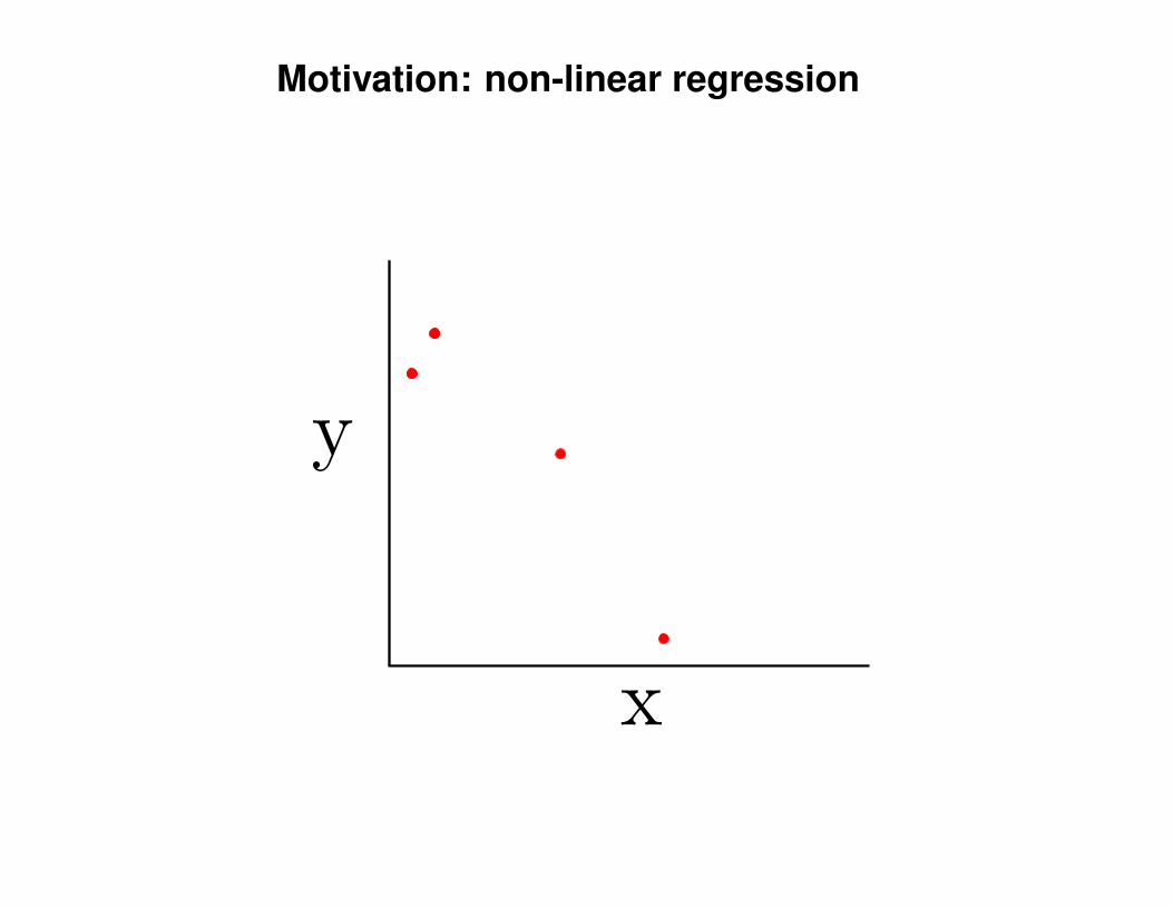
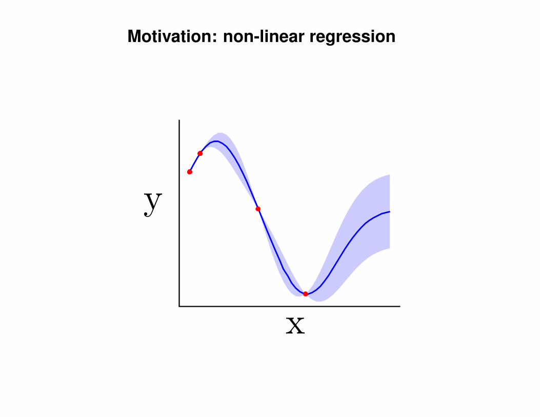
Motivation: non-linear regression
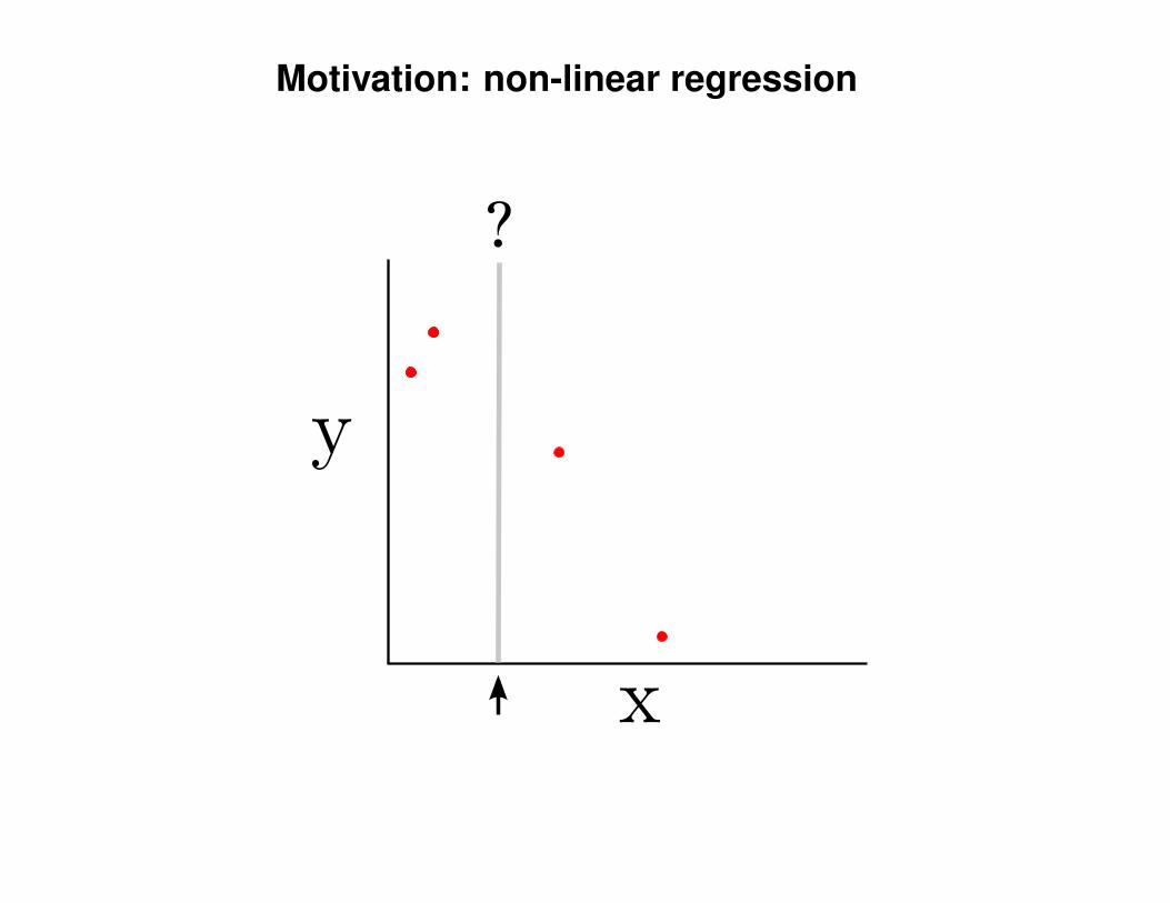
Motivation: non-linear regression
?
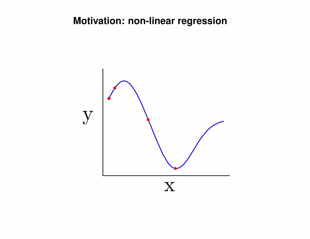
Motivation: non-linear regression
Motivation: non-linear regression
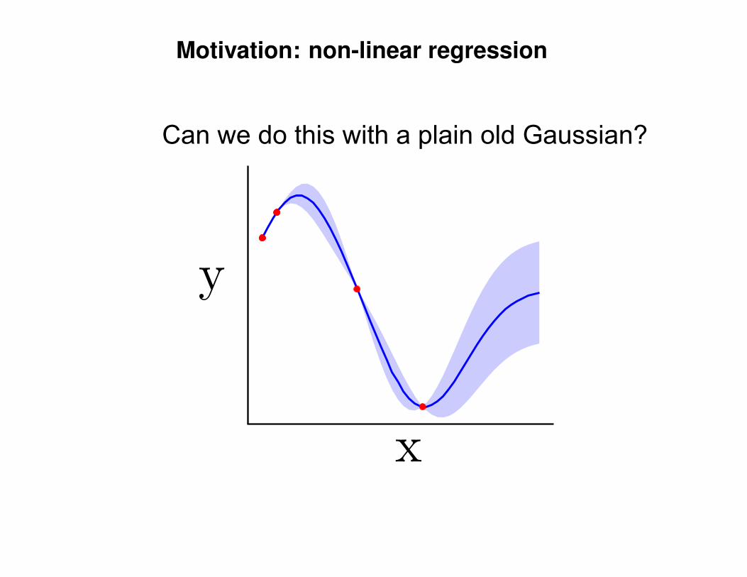
Motivation: non-linear regression
Can we do this with a plain old Gaussian?

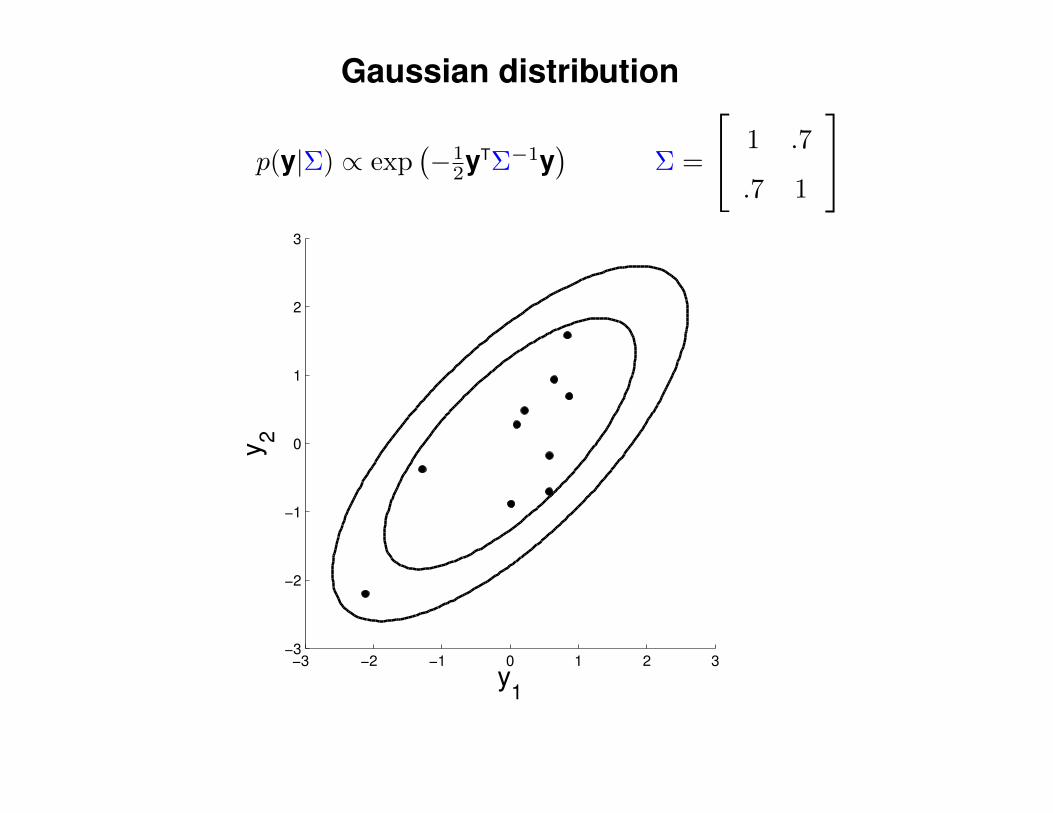
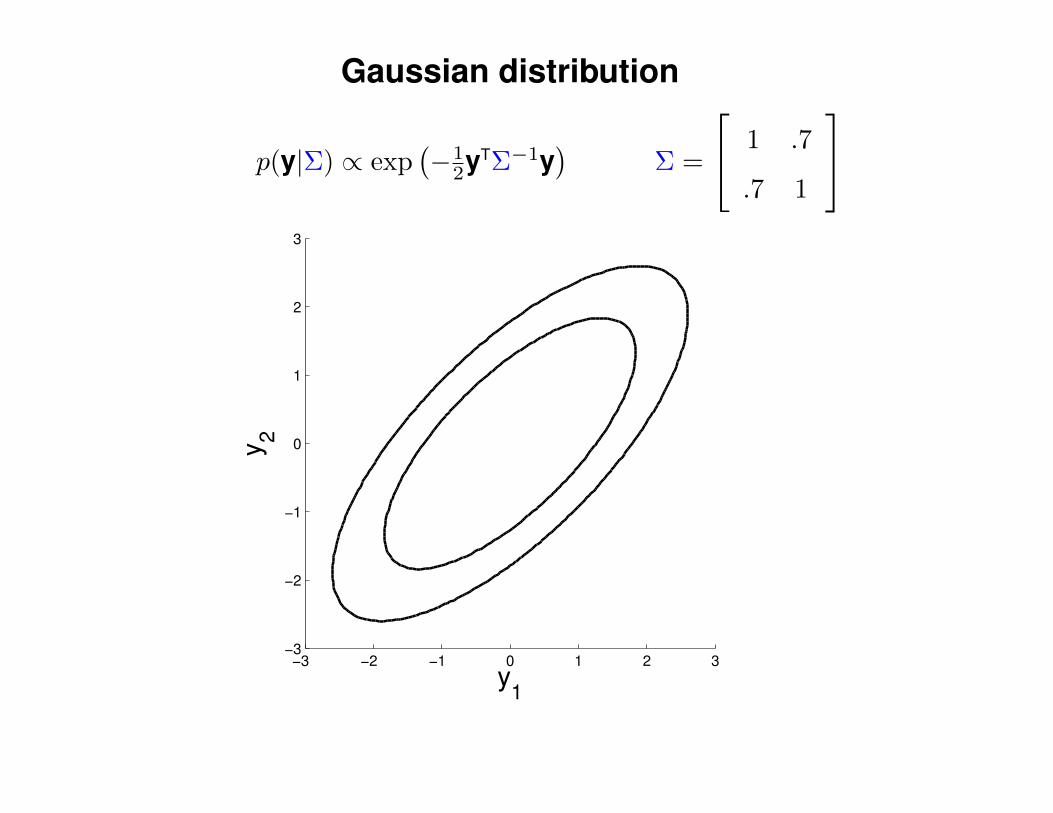
Gaussian distribution
p(y|Σ) ∝ exp(−1
2yTΣ−1y)
Σ =
1 .7
.7 1
y1
y2
−3 −2 −1 0 1 2 3−3
−2
−1
0
1
2
3
Gaussian distribution
p(y|Σ) ∝ exp(−1
2yTΣ−1y)
Σ =
1 .7
.7 1
y1
y2
−3 −2 −1 0 1 2 3−3
−2
−1
0
1
2
3
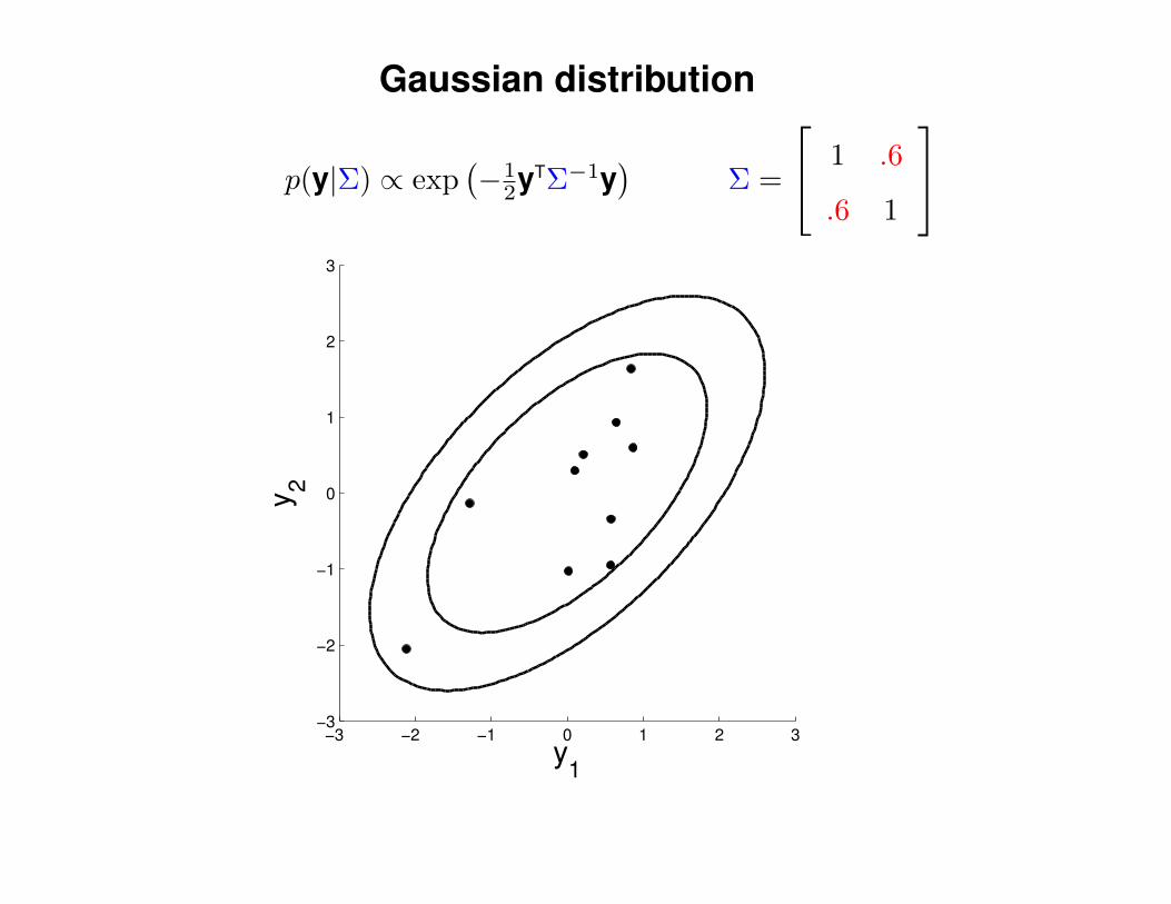
Gaussian distribution
p(y|Σ) ∝ exp(−1
2yTΣ−1y)
Σ =
1 .6
.6 1
y1
y2
−3 −2 −1 0 1 2 3−3
−2
−1
0
1
2
3
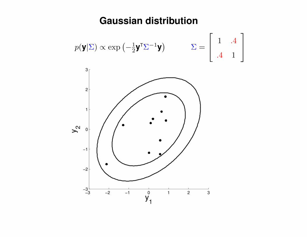
Gaussian distribution
p(y|Σ) ∝ exp(−1
2yTΣ−1y)
Σ =
1 .4
.4 1
y1
y2
−3 −2 −1 0 1 2 3−3
−2
−1
0
1
2
3

Gaussian distribution
p(y|Σ) ∝ exp(−1
2yTΣ−1y)
Σ =
1 .1
.1 1
y1
y2
−3 −2 −1 0 1 2 3−3
−2
−1
0
1
2
3
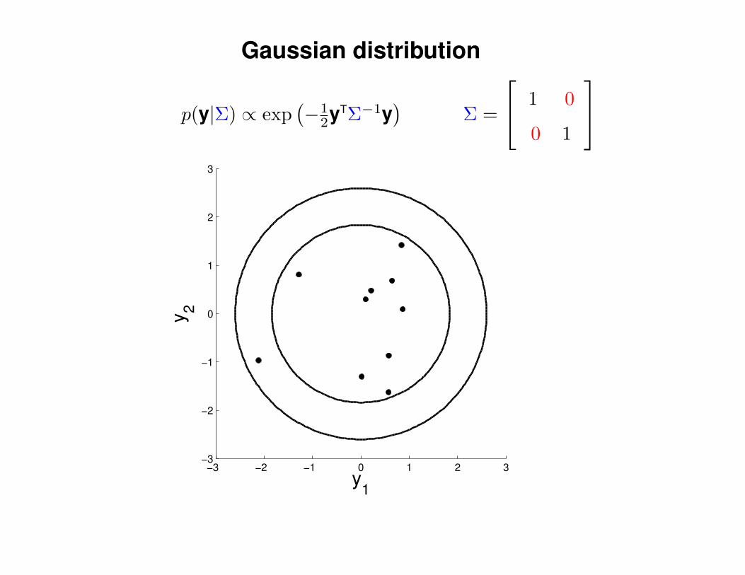
Gaussian distribution
p(y|Σ) ∝ exp(−1
2yTΣ−1y)
Σ =
1 .0
.0 1
y1
y2
−3 −2 −1 0 1 2 3−3
−2
−1
0
1
2
3
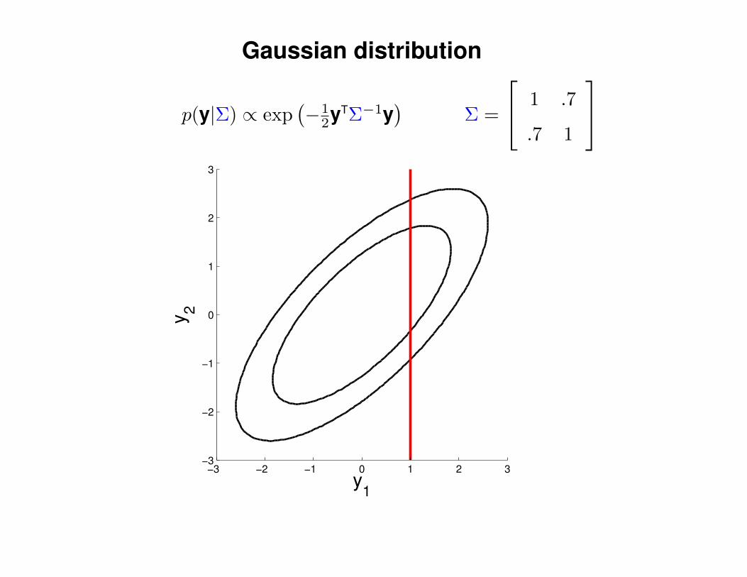
Gaussian distribution
p(y|Σ) ∝ exp(−1
2yTΣ−1y)
Σ =
1 .7
.7 1
y1
y2
−3 −2 −1 0 1 2 3−3
−2
−1
0
1
2
3
Gaussian distribution
p(y|Σ) ∝ exp(−1
2yTΣ−1y)
Σ =
1 .7
.7 1
y1
y2
−3 −2 −1 0 1 2 3−3
−2
−1
0
1
2
3
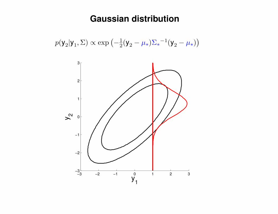
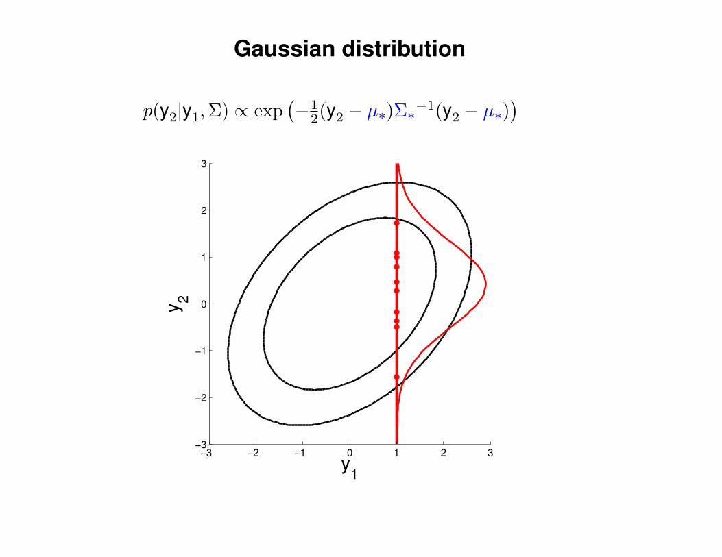
Gaussian distribution
p(y2|y1,Σ) ∝ exp(−1
2(y2 − µ∗)Σ∗−1(y2 − µ∗)) 1
2
y1
y2
−3 −2 −1 0 1 2 3−3
−2
−1
0
1
2
3
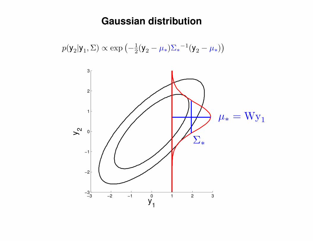
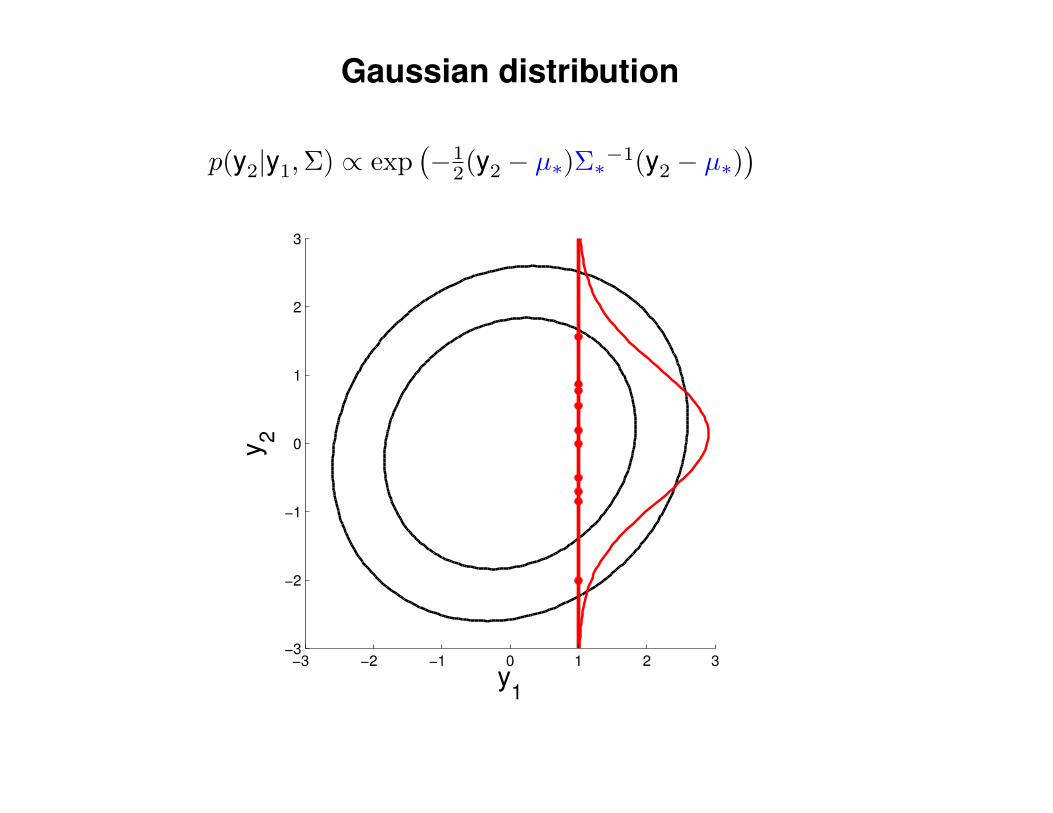
Gaussian distribution
p(y2|y1,Σ) ∝ exp(−1
2(y2 − µ∗)Σ∗−1(y2 − µ∗)) 1
2
y1
y 2
−3 −2 −1 0 1 2 3−3
−2
−1
0
1
2
3
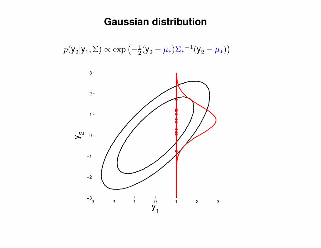
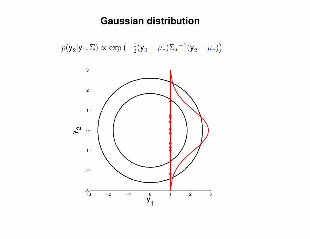
Gaussian distribution
p(y2|y1,Σ) ∝ exp(−1
2(y2 − µ∗)Σ∗−1(y2 − µ∗)) 1
2
y1
y2
−3 −2 −1 0 1 2 3−3
−2
−1
0
1
2
3
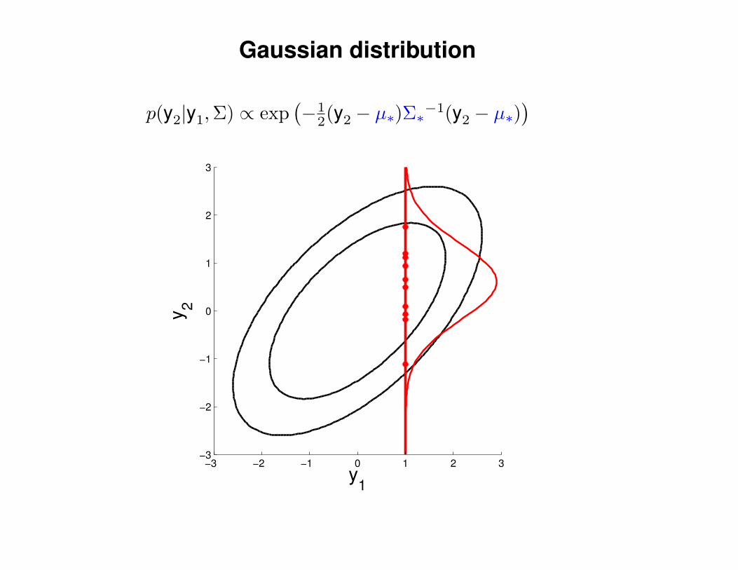
Gaussian distribution
p(y2|y1,Σ) ∝ exp(−1
2(y2 − µ∗)Σ∗−1(y2 − µ∗)) 1
2
y1
y2
−3 −2 −1 0 1 2 3−3
−2
−1
0
1
2
3
Gaussian distribution
p(y2|y1,Σ) ∝ exp(−1
2(y2 − µ∗)Σ∗−1(y2 − µ∗)) 1
2
y1
y2
−3 −2 −1 0 1 2 3−3
−2
−1
0
1
2
3
Gaussian distribution
p(y2|y1,Σ) ∝ exp(−1
2(y2 − µ∗)Σ∗−1(y2 − µ∗)) 1
2
y1
y2
−3 −2 −1 0 1 2 3−3
−2
−1
0
1
2
3
Gaussian distribution
p(y2|y1,Σ) ∝ exp(−1
2(y2 − µ∗)Σ∗−1(y2 − µ∗)) 1
2
y1
y2
−3 −2 −1 0 1 2 3−3
−2
−1
0
1
2
3
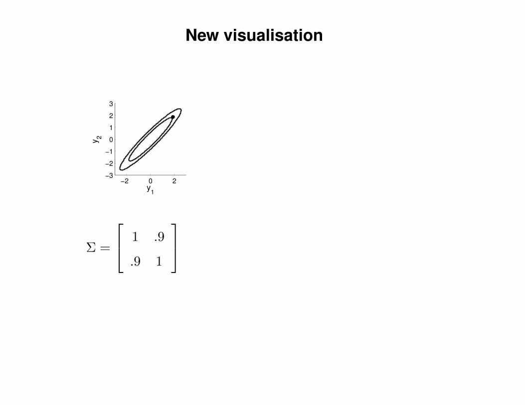
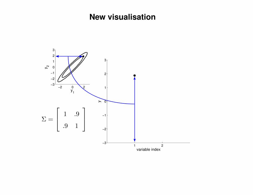
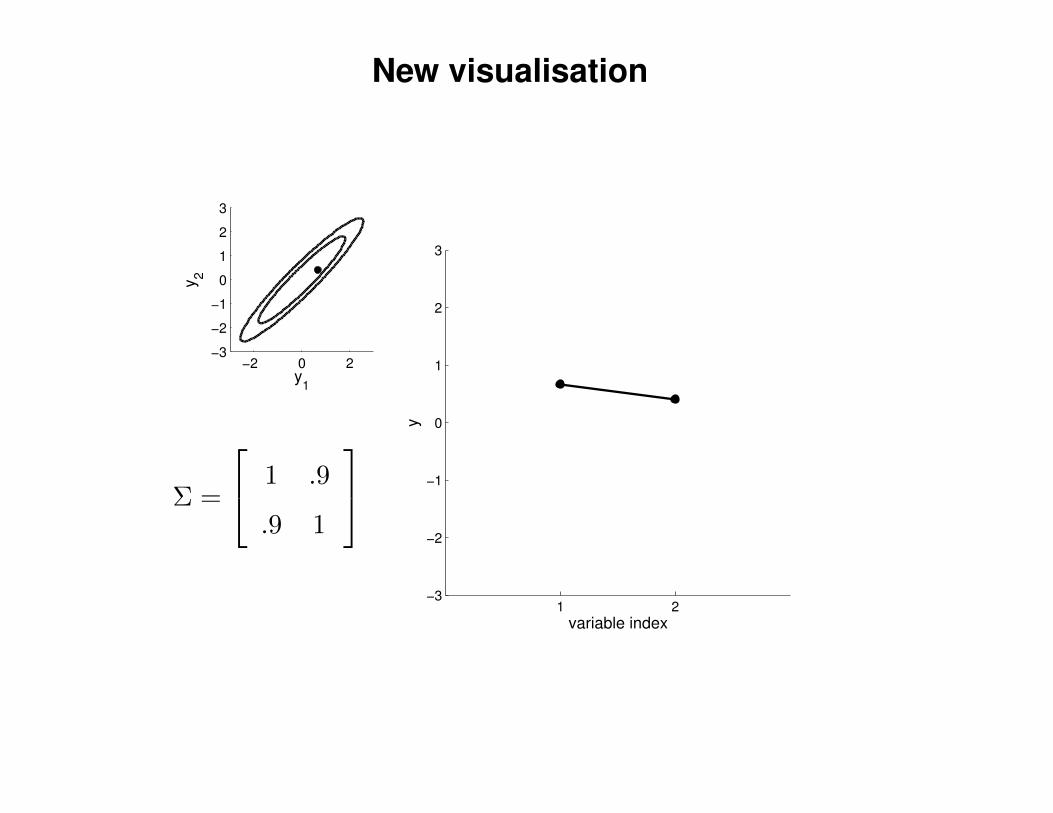
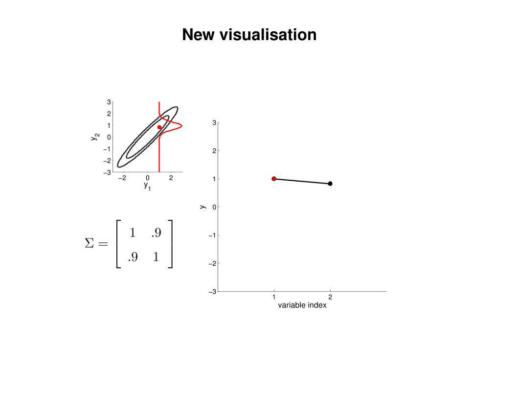
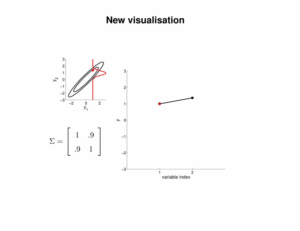
New visualisation
−2 0 2−3
−2
−1
0
1
2
3
y1
y 2
Σ =
1 .9
.9 1
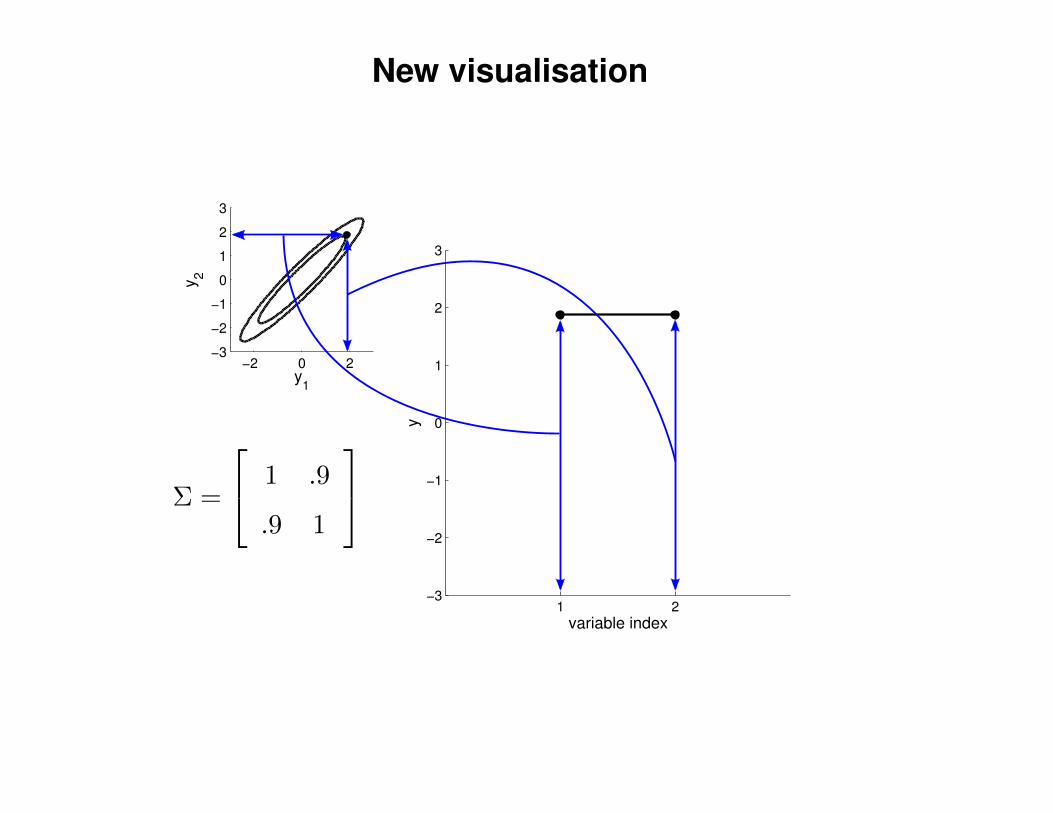
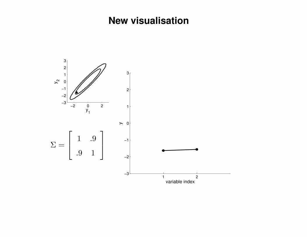
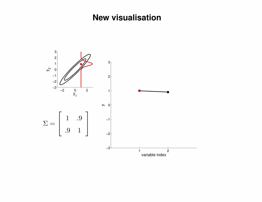
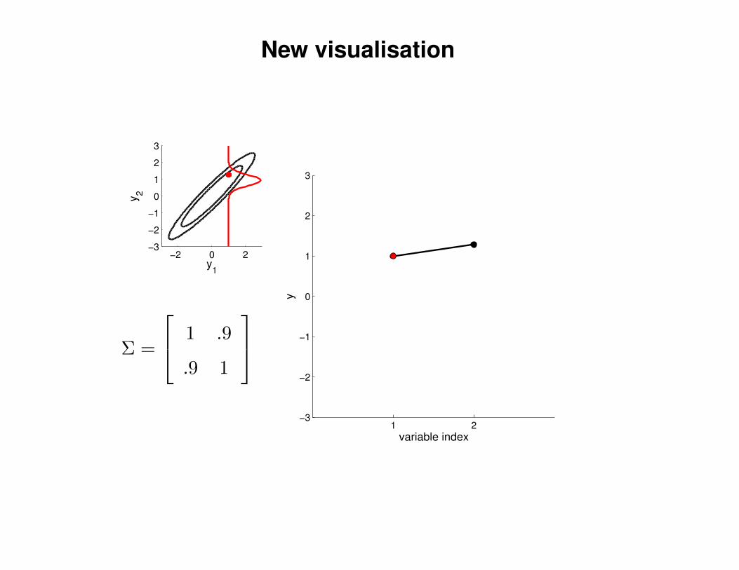
New visualisation
−2 0 2−3
−2
−1
0
1
2
3
y1
y 2
1 2−3
−2
−1
0
1
2
3
variable index
y
Σ =
1 .9
.9 1
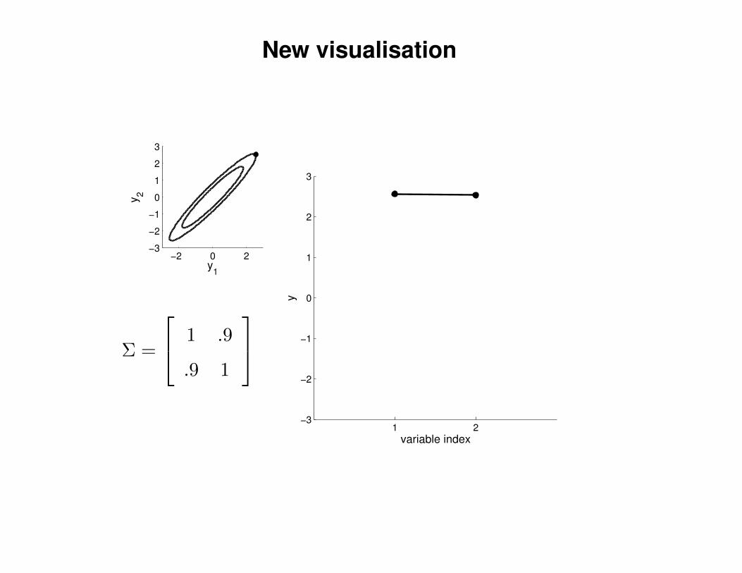
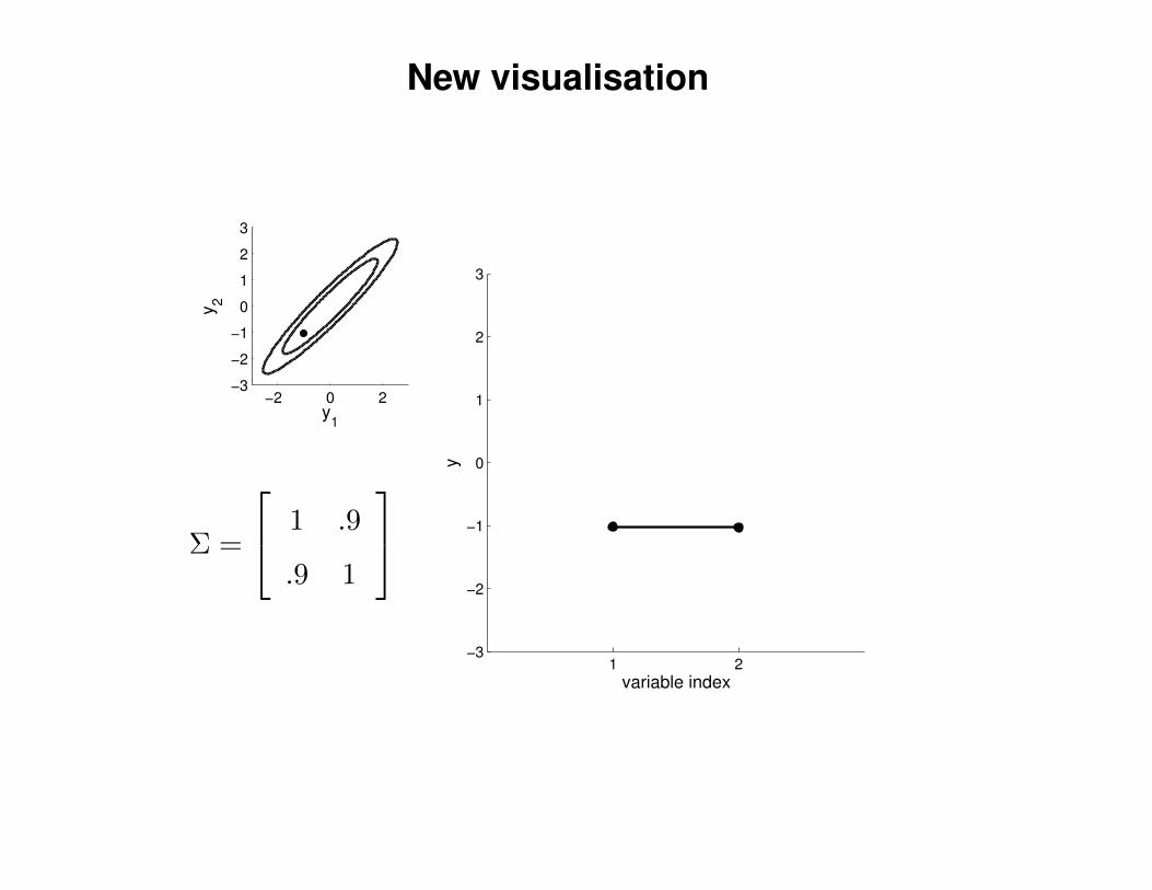
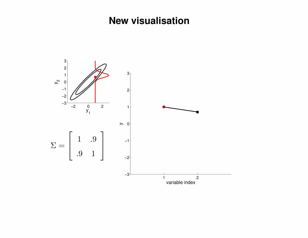
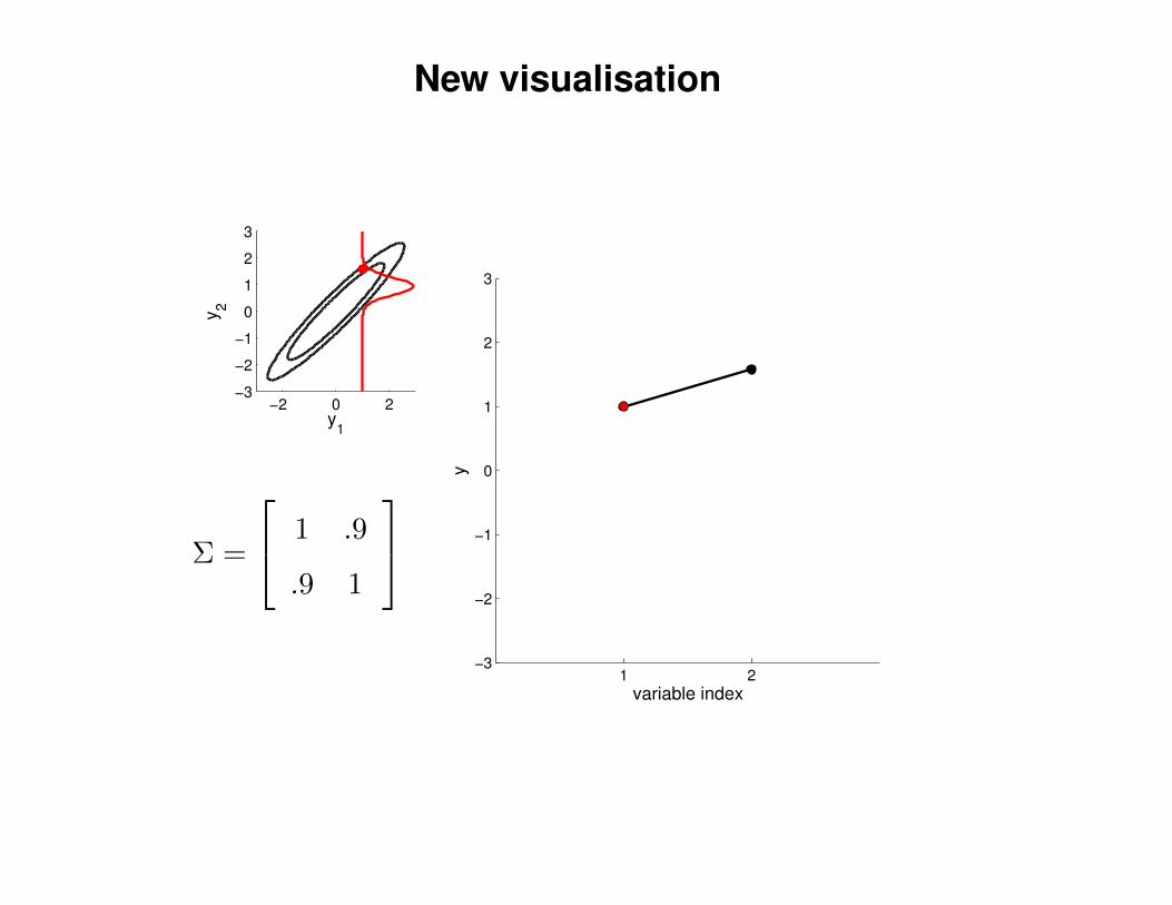
New visualisation
−2 0 2−3
−2
−1
0
1
2
3
y1
y 2
1 2−3
−2
−1
0
1
2
3
variable index
y
Σ =
1 .9
.9 1

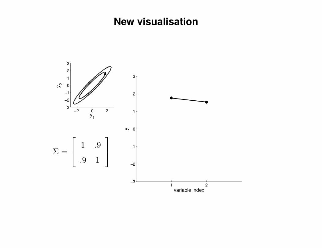
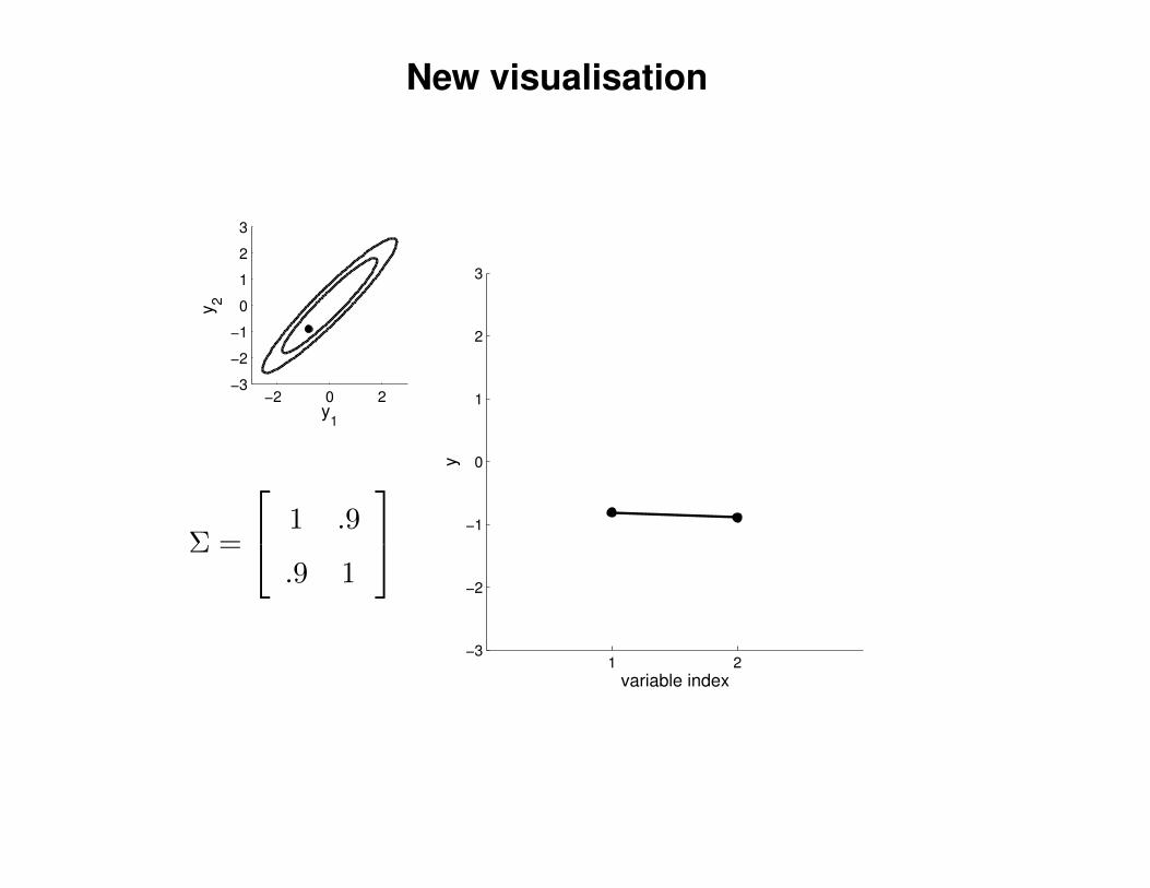
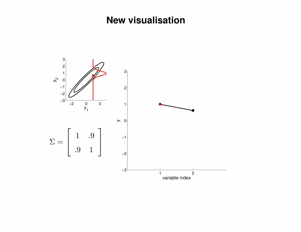
New visualisation
−2 0 2−3
−2
−1
0
1
2
3
y1
y2
1 2−3
−2
−1
0
1
2
3
variable index
y
Σ =
1 .9
.9 1

New visualisation
−2 0 2−3
−2
−1
0
1
2
3
y1
y2
1 2−3
−2
−1
0
1
2
3
variable index
y
Σ =
1 .9
.9 1
New visualisation
−2 0 2−3
−2
−1
0
1
2
3
y1
y2
1 2−3
−2
−1
0
1
2
3
variable index
y
Σ =
1 .9
.9 1

New visualisation
−2 0 2−3
−2
−1
0
1
2
3
y1
y2
1 2−3
−2
−1
0
1
2
3
variable index
y
Σ =
1 .9
.9 1

New visualisation
−2 0 2−3
−2
−1
0
1
2
3
y1
y2
1 2−3
−2
−1
0
1
2
3
variable index
y
Σ =
1 .9
.9 1
New visualisation
−2 0 2−3
−2
−1
0
1
2
3
y1
y2
1 2−3
−2
−1
0
1
2
3
variable index
y
Σ =
1 .9
.9 1
New visualisation
−2 0 2−3
−2
−1
0
1
2
3
y1
y2
1 2−3
−2
−1
0
1
2
3
variable index
y
Σ =
1 .9
.9 1

New visualisation
−2 0 2−3
−2
−1
0
1
2
3
y1
y2
1 2−3
−2
−1
0
1
2
3
variable index
y
Σ =
1 .9
.9 1

New visualisation
−2 0 2−3
−2
−1
0
1
2
3
y1
y2
1 2−3
−2
−1
0
1
2
3
variable index
y
Σ =
1 .9
.9 1

New visualisation
−2 0 2−3
−2
−1
0
1
2
3
y1
y2
1 2−3
−2
−1
0
1
2
3
variable index
y
Σ =
1 .9
.9 1

New visualisation
−2 0 2−3
−2
−1
0
1
2
3
y1
y2
1 2−3
−2
−1
0
1
2
3
variable index
y
Σ =
1 .9
.9 1

New visualisation
−2 0 2−3
−2
−1
0
1
2
3
y1
y2
1 2−3
−2
−1
0
1
2
3
variable index
y
Σ =
1 .9
.9 1

New visualisation
−2 0 2−3
−2
−1
0
1
2
3
y1
y2
1 2−3
−2
−1
0
1
2
3
variable index
y
Σ =
1 .9
.9 1
New visualisation
−2 0 2−3
−2
−1
0
1
2
3
y1
y2
1 2−3
−2
−1
0
1
2
3
variable index
y
Σ =
1 .9
.9 1

New visualisation
−2 0 2−3
−2
−1
0
1
2
3
y1
y2
1 2−3
−2
−1
0
1
2
3
variable index
y
Σ =
1 .9
.9 1
New visualisation
−2 0 2−3
−2
−1
0
1
2
3
y1
y2
1 2−3
−2
−1
0
1
2
3
variable index
y
Σ =
1 .9
.9 1
New visualisation
−2 0 2−3
−2
−1
0
1
2
3
y1
y2
1 2−3
−2
−1
0
1
2
3
variable index
y
Σ =
1 .9
.9 1

New visualisation
−2 0 2−3
−2
−1
0
1
2
3
y1
y2
1 2−3
−2
−1
0
1
2
3
variable index
y
Σ =
1 .9
.9 1

New visualisation
−2 0 2−3
−2
−1
0
1
2
3
y1
y2
1 2−3
−2
−1
0
1
2
3
variable index
y
Σ =
1 .9
.9 1

New visualisation
−2 0 2−3
−2
−1
0
1
2
3
y1
y2
1 2−3
−2
−1
0
1
2
3
variable index
y
Σ =
1 .9
.9 1

New visualisation
−2 0 2−3
−2
−1
0
1
2
3
y1
y2
1 2−3
−2
−1
0
1
2
3
variable index
y
Σ =
1 .9
.9 1
New visualisation
−2 0 2−3
−2
−1
0
1
2
3
y1
y2
1 2−3
−2
−1
0
1
2
3
variable index
y
Σ =
1 .9
.9 1
New visualisation
−2 0 2−3
−2
−1
0
1
2
3
y1
y2
1 2−3
−2
−1
0
1
2
3
variable index
y
Σ =
1 .9
.9 1

New visualisation
−2 0 2−3
−2
−1
0
1
2
3
y1
y2
1 2−3
−2
−1
0
1
2
3
variable index
y
Σ =
1 .9
.9 1

New visualisation
−2 0 2−3
−2
−1
0
1
2
3
y1
y2
1 2−3
−2
−1
0
1
2
3
variable index
y
Σ =
1 .9
.9 1

New visualisation
−2 0 2−3
−2
−1
0
1
2
3
y1
y2
1 2−3
−2
−1
0
1
2
3
variable index
y
Σ =
1 .9
.9 1

New visualisation
−2 0 2−3
−2
−1
0
1
2
3
y1
y2
1 2−3
−2
−1
0
1
2
3
variable index
y
Σ =
1 .9
.9 1

New visualisation
−2 0 2−3
−2
−1
0
1
2
3
y1
y2
1 2−3
−2
−1
0
1
2
3
variable index
y
Σ =
1 .9
.9 1

New visualisation
−2 0 2−3
−2
−1
0
1
2
3
y1
y2
1 2−3
−2
−1
0
1
2
3
variable index
y
Σ =
1 .9
.9 1

New visualisation
−2 0 2−3
−2
−1
0
1
2
3
y1
y2
1 2−3
−2
−1
0
1
2
3
variable index
y
Σ =
1 .9
.9 1

New visualisation
−2 0 2−3
−2
−1
0
1
2
3
y1
y2
1 2−3
−2
−1
0
1
2
3
variable index
y
Σ =
1 .9
.9 1
New visualisation
−2 0 2−3
−2
−1
0
1
2
3
y1
y2
1 2−3
−2
−1
0
1
2
3
variable index
y
Σ =
1 .9
.9 1
New visualisation
−2 0 2−3
−2
−1
0
1
2
3
y1
y2
1 2−3
−2
−1
0
1
2
3
variable index
y
Σ =
1 .9
.9 1

New visualisation
−2 0 2−3
−2
−1
0
1
2
3
y1
y2
1 2−3
−2
−1
0
1
2
3
variable index
y
Σ =
1 .9
.9 1

New visualisation
−2 0 2−3
−2
−1
0
1
2
3
y1
y2
1 2−3
−2
−1
0
1
2
3
variable index
y
Σ =
1 .9
.9 1
New visualisation
−2 0 2−3
−2
−1
0
1
2
3
y1
y2
1 2−3
−2
−1
0
1
2
3
variable index
y
Σ =
1 .9
.9 1
New visualisation
−2 0 2−3
−2
−1
0
1
2
3
y1
y2
1 2−3
−2
−1
0
1
2
3
variable index
y
Σ =
1 .9
.9 1

New visualisation
−2 0 2−3
−2
−1
0
1
2
3
y1
y2
1 2−3
−2
−1
0
1
2
3
variable index
y
Σ =
1 .9
.9 1

New visualisation
−2 0 2−3
−2
−1
0
1
2
3
y1
y2
1 2−3
−2
−1
0
1
2
3
variable index
y
Σ =
1 .9
.9 1
New visualisation
−2 0 2−3
−2
−1
0
1
2
3
y1
y2
1 2−3
−2
−1
0
1
2
3
variable index
y
Σ =
1 .9
.9 1
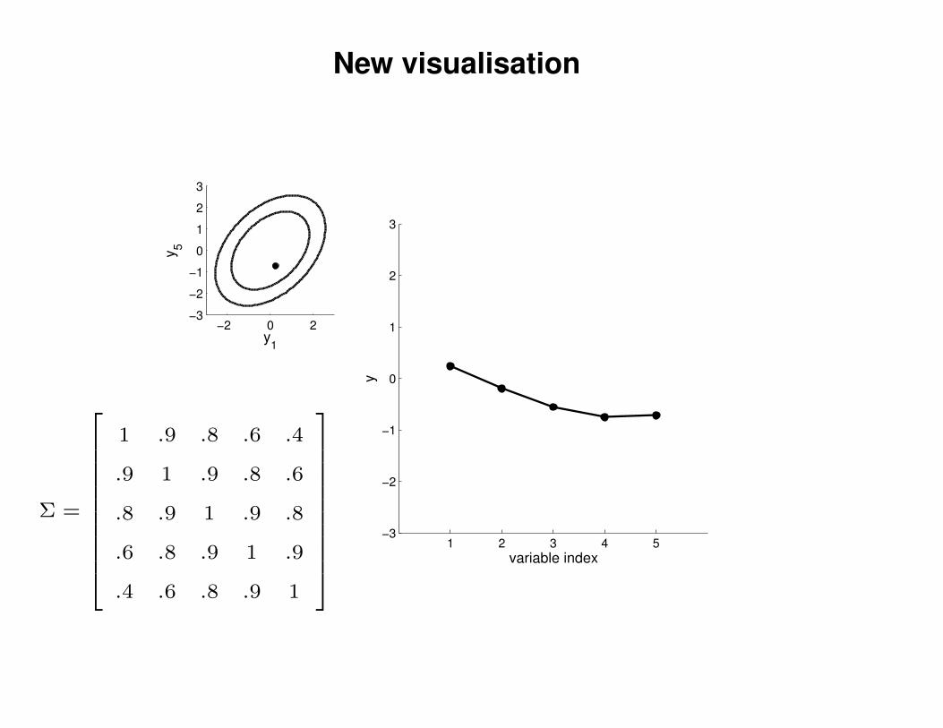
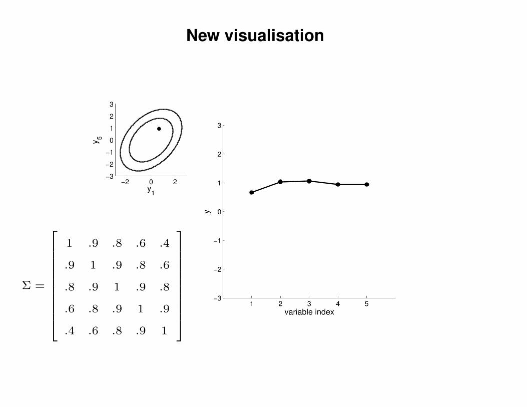
New visualisation
−2 0 2−3
−2
−1
0
1
2
3
y1
y5
1 2 3 4 5−3
−2
−1
0
1
2
3
variable index
y
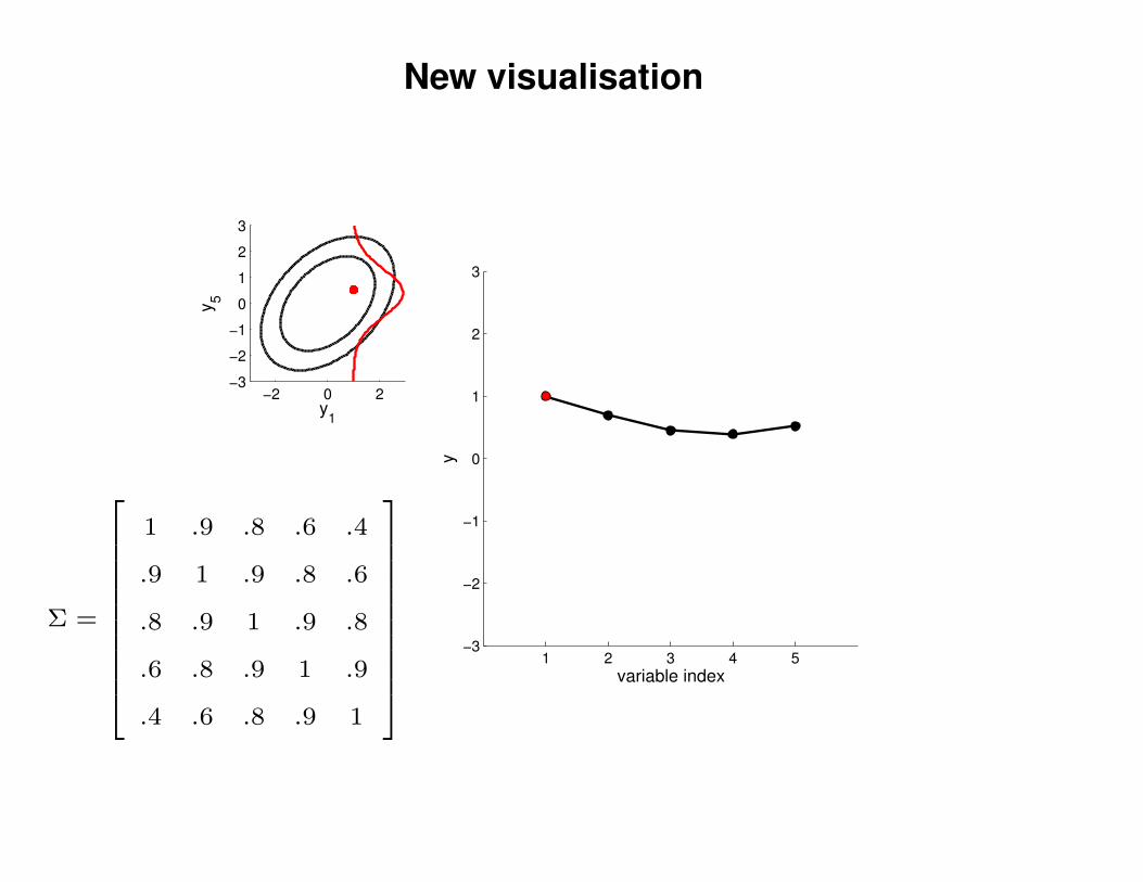
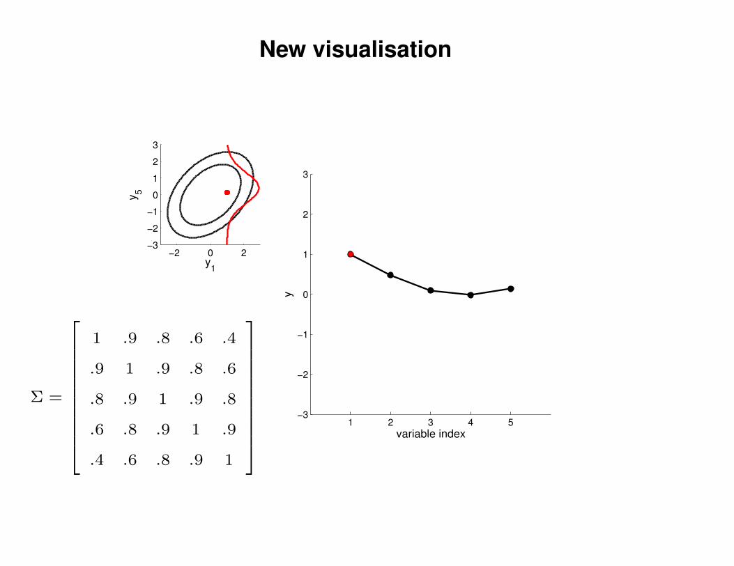
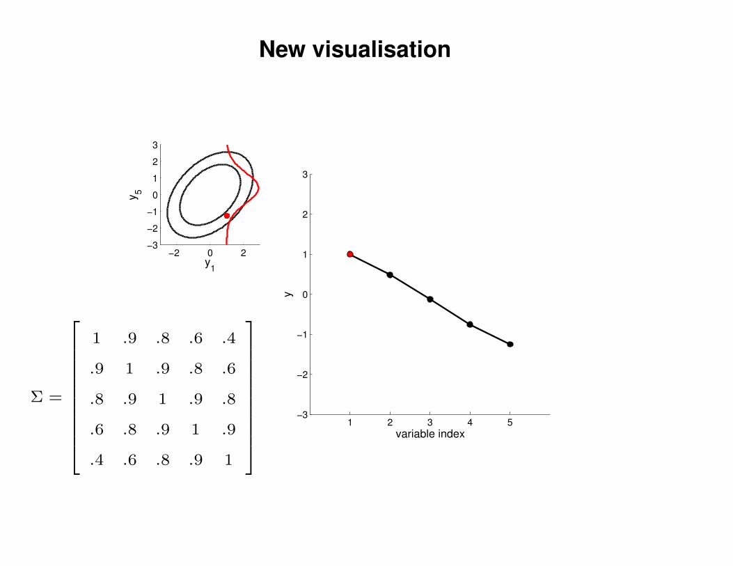
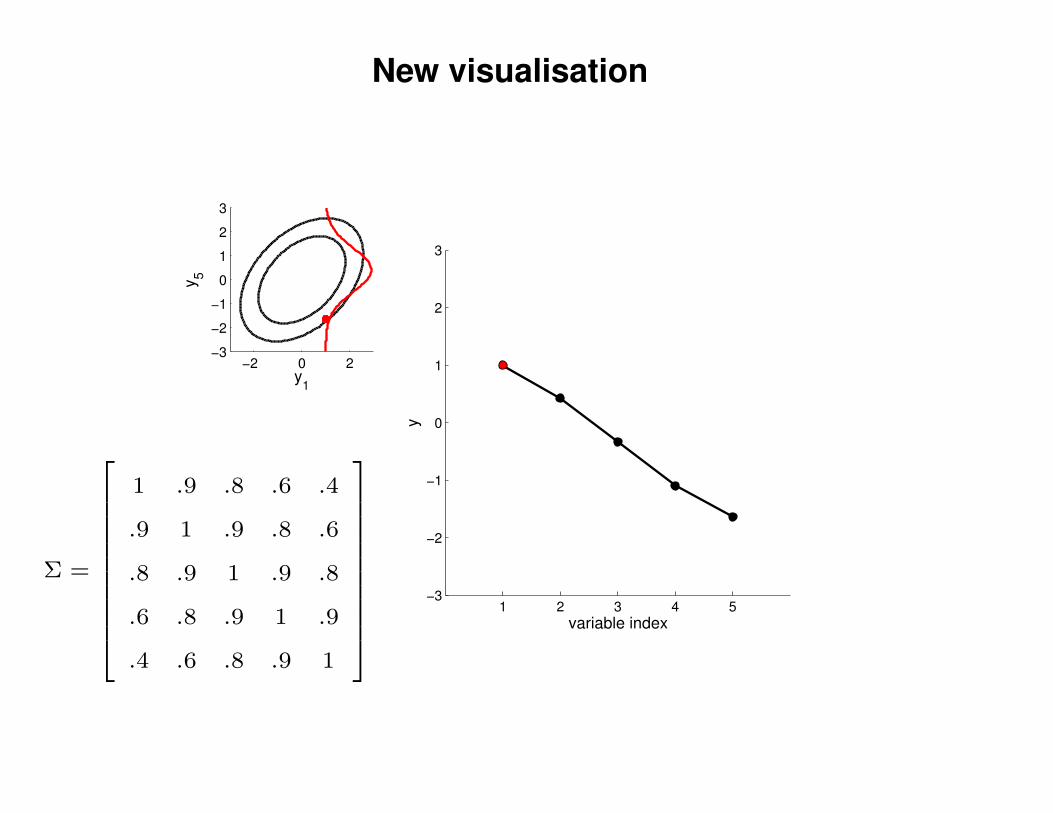
Σ =
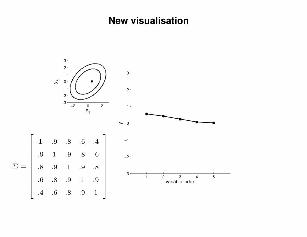
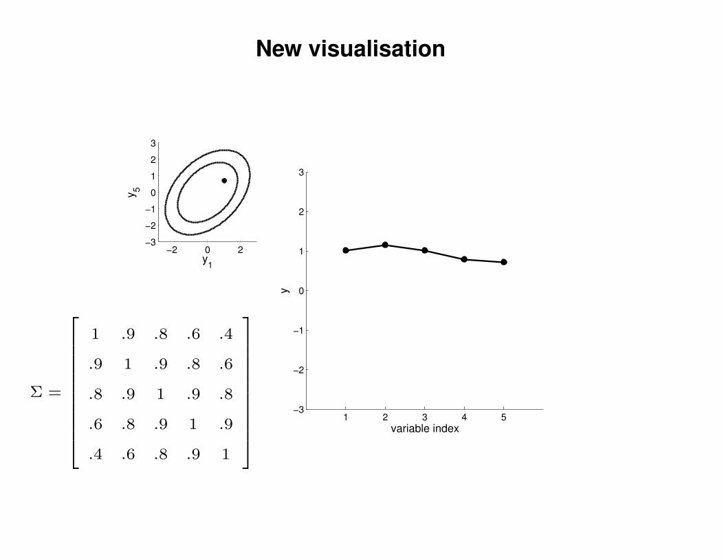
1 .9 .8 .6 .4
.9 1 .9 .8 .6
.8 .9 1 .9 .8
.6 .8 .9 1 .9
.4 .6 .8 .9 1
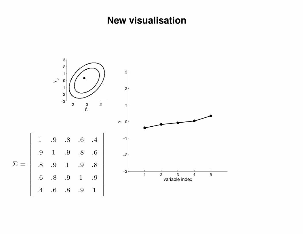
New visualisation
−2 0 2−3
−2
−1
0
1
2
3
y1
y5
1 2 3 4 5−3
−2
−1
0
1
2
3
variable index
y
Σ =
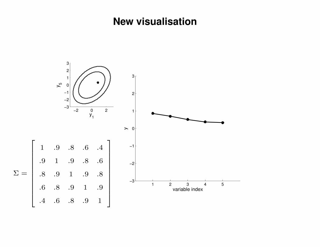
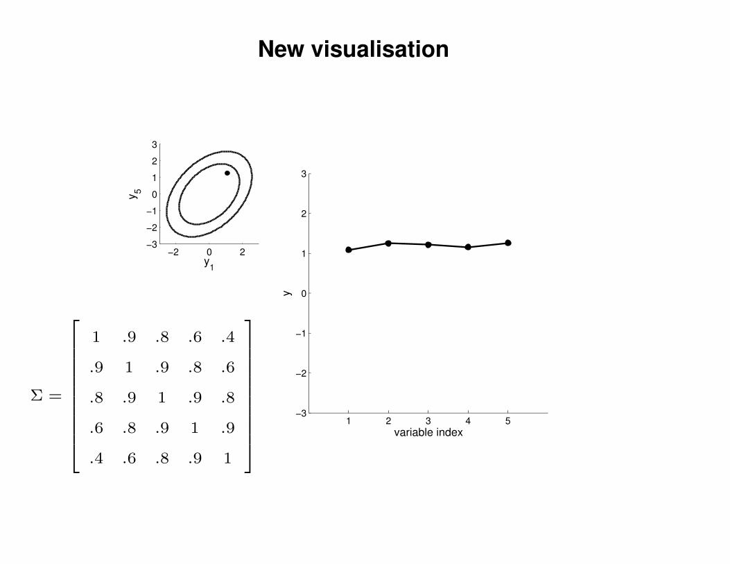
1 .9 .8 .6 .4
.9 1 .9 .8 .6
.8 .9 1 .9 .8
.6 .8 .9 1 .9
.4 .6 .8 .9 1
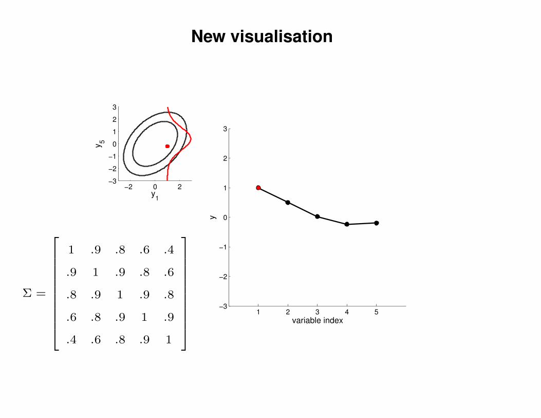
New visualisation
−2 0 2−3
−2
−1
0
1
2
3
y1
y5
1 2 3 4 5−3
−2
−1
0
1
2
3
variable index
y
Σ =
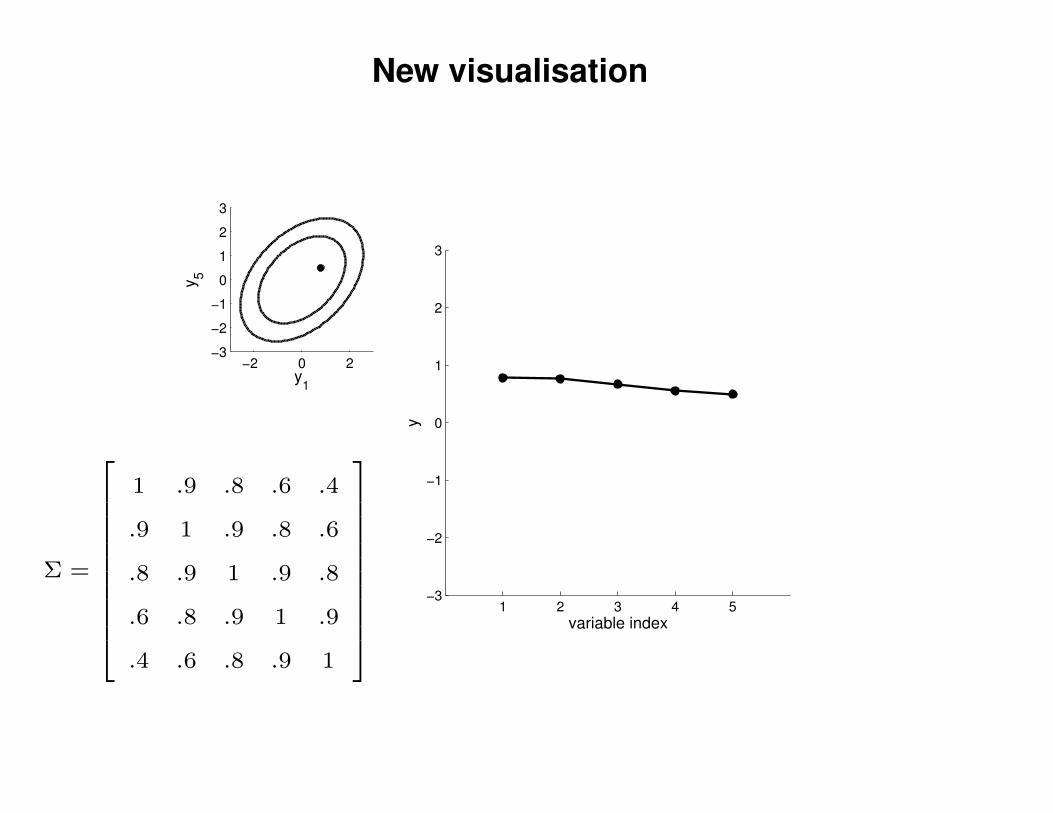
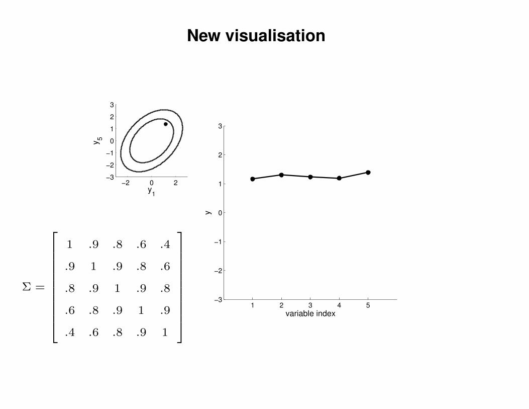
1 .9 .8 .6 .4
.9 1 .9 .8 .6
.8 .9 1 .9 .8
.6 .8 .9 1 .9
.4 .6 .8 .9 1
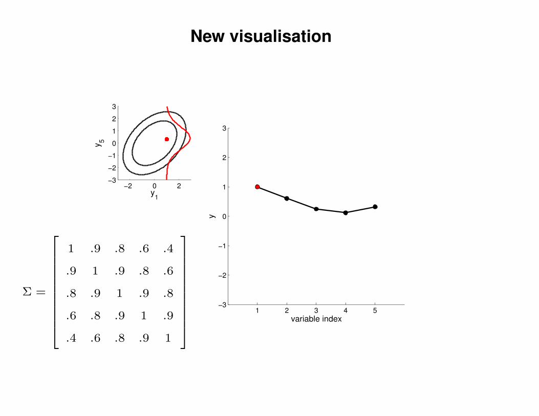
New visualisation
−2 0 2−3
−2
−1
0
1
2
3
y1
y5
1 2 3 4 5−3
−2
−1
0
1
2
3
variable index
y
Σ =
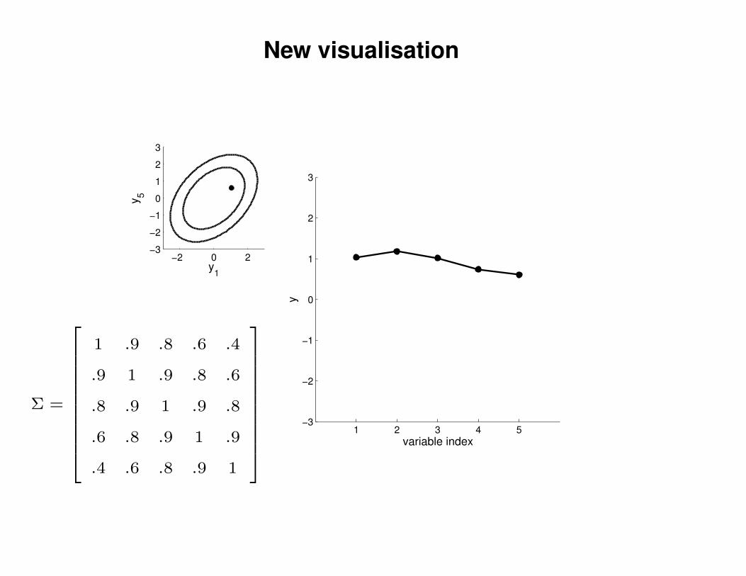
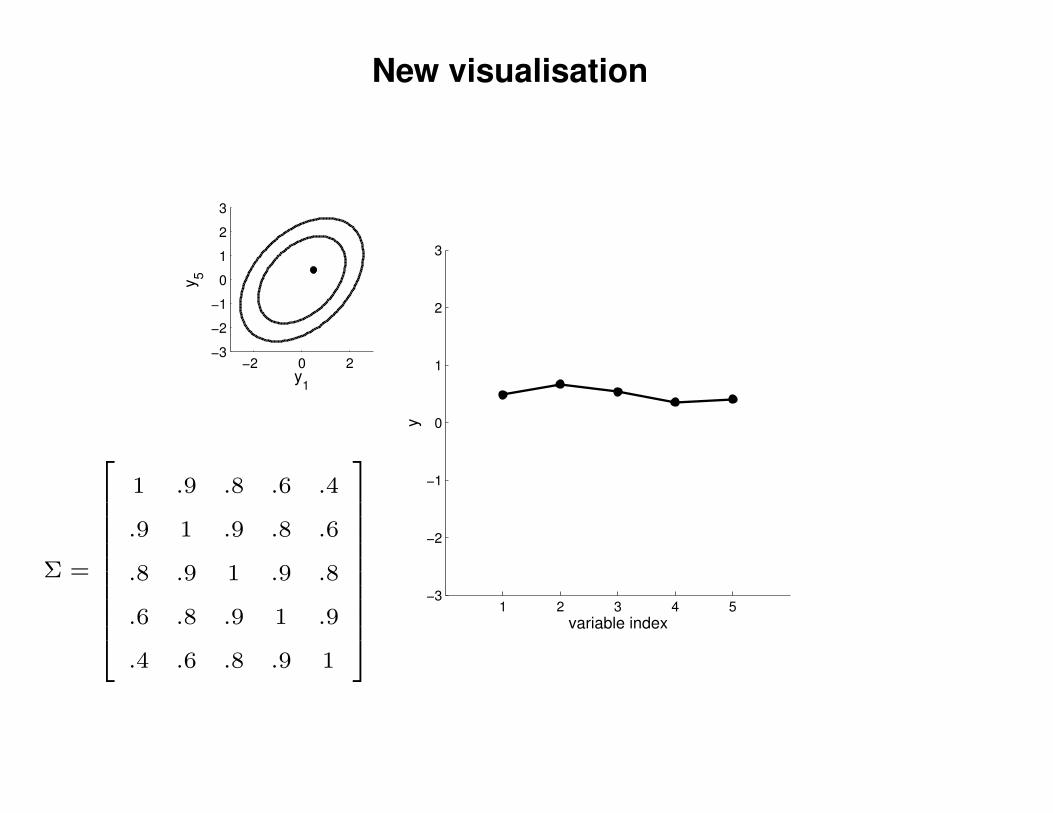
1 .9 .8 .6 .4
.9 1 .9 .8 .6
.8 .9 1 .9 .8
.6 .8 .9 1 .9
.4 .6 .8 .9 1

New visualisation
−2 0 2−3
−2
−1
0
1
2
3
y1
y5
1 2 3 4 5−3
−2
−1
0
1
2
3
variable index
y
Σ =
1 .9 .8 .6 .4
.9 1 .9 .8 .6
.8 .9 1 .9 .8
.6 .8 .9 1 .9
.4 .6 .8 .9 1

New visualisation
−2 0 2−3
−2
−1
0
1
2
3
y1
y5
1 2 3 4 5−3
−2
−1
0
1
2
3
variable index
y
Σ =
1 .9 .8 .6 .4
.9 1 .9 .8 .6
.8 .9 1 .9 .8
.6 .8 .9 1 .9
.4 .6 .8 .9 1

New visualisation
−2 0 2−3
−2
−1
0
1
2
3
y1
y5
1 2 3 4 5−3
−2
−1
0
1
2
3
variable index
y
Σ =
1 .9 .8 .6 .4
.9 1 .9 .8 .6
.8 .9 1 .9 .8
.6 .8 .9 1 .9
.4 .6 .8 .9 1

New visualisation
−2 0 2−3
−2
−1
0
1
2
3
y1
y5
1 2 3 4 5−3
−2
−1
0
1
2
3
variable index
y
Σ =
1 .9 .8 .6 .4
.9 1 .9 .8 .6
.8 .9 1 .9 .8
.6 .8 .9 1 .9
.4 .6 .8 .9 1

New visualisation
−2 0 2−3
−2
−1
0
1
2
3
y1
y5
1 2 3 4 5−3
−2
−1
0
1
2
3
variable index
y
Σ =
1 .9 .8 .6 .4
.9 1 .9 .8 .6
.8 .9 1 .9 .8
.6 .8 .9 1 .9
.4 .6 .8 .9 1
New visualisation
−2 0 2−3
−2
−1
0
1
2
3
y1
y5
1 2 3 4 5−3
−2
−1
0
1
2
3
variable index
y
Σ =
1 .9 .8 .6 .4
.9 1 .9 .8 .6
.8 .9 1 .9 .8
.6 .8 .9 1 .9
.4 .6 .8 .9 1
New visualisation
−2 0 2−3
−2
−1
0
1
2
3
y1
y5
1 2 3 4 5−3
−2
−1
0
1
2
3
variable index
y
Σ =
1 .9 .8 .6 .4
.9 1 .9 .8 .6
.8 .9 1 .9 .8
.6 .8 .9 1 .9
.4 .6 .8 .9 1
New visualisation
−2 0 2−3
−2
−1
0
1
2
3
y1
y5
1 2 3 4 5−3
−2
−1
0
1
2
3
variable index
y
Σ =
1 .9 .8 .6 .4
.9 1 .9 .8 .6
.8 .9 1 .9 .8
.6 .8 .9 1 .9
.4 .6 .8 .9 1

New visualisation
−2 0 2−3
−2
−1
0
1
2
3
y1
y5
1 2 3 4 5−3
−2
−1
0
1
2
3
variable index
y
Σ =
1 .9 .8 .6 .4
.9 1 .9 .8 .6
.8 .9 1 .9 .8
.6 .8 .9 1 .9
.4 .6 .8 .9 1
New visualisation
−2 0 2−3
−2
−1
0
1
2
3
y1
y5
1 2 3 4 5−3
−2
−1
0
1
2
3
variable index
y
Σ =
1 .9 .8 .6 .4
.9 1 .9 .8 .6
.8 .9 1 .9 .8
.6 .8 .9 1 .9
.4 .6 .8 .9 1

New visualisation
−2 0 2−3
−2
−1
0
1
2
3
y1
y5
1 2 3 4 5−3
−2
−1
0
1
2
3
variable index
y
Σ =
1 .9 .8 .6 .4
.9 1 .9 .8 .6
.8 .9 1 .9 .8
.6 .8 .9 1 .9
.4 .6 .8 .9 1
New visualisation
−2 0 2−3
−2
−1
0
1
2
3
y1
y5
1 2 3 4 5−3
−2
−1
0
1
2
3
variable index
y
Σ =
1 .9 .8 .6 .4
.9 1 .9 .8 .6
.8 .9 1 .9 .8
.6 .8 .9 1 .9
.4 .6 .8 .9 1
New visualisation
−2 0 2−3
−2
−1
0
1
2
3
y1
y5
1 2 3 4 5−3
−2
−1
0
1
2
3
variable index
y
Σ =
1 .9 .8 .6 .4
.9 1 .9 .8 .6
.8 .9 1 .9 .8
.6 .8 .9 1 .9
.4 .6 .8 .9 1

New visualisation
−2 0 2−3
−2
−1
0
1
2
3
y1
y5
1 2 3 4 5−3
−2
−1
0
1
2
3
variable index
y
Σ =
1 .9 .8 .6 .4
.9 1 .9 .8 .6
.8 .9 1 .9 .8
.6 .8 .9 1 .9
.4 .6 .8 .9 1

New visualisation
−2 0 2−3
−2
−1
0
1
2
3
y1
y5
1 2 3 4 5−3
−2
−1
0
1
2
3
variable index
y
Σ =
1 .9 .8 .6 .4
.9 1 .9 .8 .6
.8 .9 1 .9 .8
.6 .8 .9 1 .9
.4 .6 .8 .9 1
New visualisation
−2 0 2−3
−2
−1
0
1
2
3
y1
y5
1 2 3 4 5−3
−2
−1
0
1
2
3
variable index
y
Σ =
1 .9 .8 .6 .4
.9 1 .9 .8 .6
.8 .9 1 .9 .8
.6 .8 .9 1 .9
.4 .6 .8 .9 1

New visualisation
−2 0 2−3
−2
−1
0
1
2
3
y1
y5
1 2 3 4 5−3
−2
−1
0
1
2
3
variable index
y
Σ =
1 .9 .8 .6 .4
.9 1 .9 .8 .6
.8 .9 1 .9 .8
.6 .8 .9 1 .9
.4 .6 .8 .9 1
New visualisation
−2 0 2−3
−2
−1
0
1
2
3
y1
y5
1 2 3 4 5−3
−2
−1
0
1
2
3
variable index
y
Σ =
1 .9 .8 .6 .4
.9 1 .9 .8 .6
.8 .9 1 .9 .8
.6 .8 .9 1 .9
.4 .6 .8 .9 1
New visualisation
−2 0 2−3
−2
−1
0
1
2
3
y1
y5
1 2 3 4 5−3
−2
−1
0
1
2
3
variable index
y
Σ =
1 .9 .8 .6 .4
.9 1 .9 .8 .6
.8 .9 1 .9 .8
.6 .8 .9 1 .9
.4 .6 .8 .9 1
New visualisation
−2 0 2−3
−2
−1
0
1
2
3
y1
y5
1 2 3 4 5−3
−2
−1
0
1
2
3
variable index
y
Σ =
1 .9 .8 .6 .4
.9 1 .9 .8 .6
.8 .9 1 .9 .8
.6 .8 .9 1 .9
.4 .6 .8 .9 1
New visualisation
−2 0 2−3
−2
−1
0
1
2
3
y1
y5
1 2 3 4 5−3
−2
−1
0
1
2
3
variable index
y
Σ =
1 .9 .8 .6 .4
.9 1 .9 .8 .6
.8 .9 1 .9 .8
.6 .8 .9 1 .9
.4 .6 .8 .9 1

New visualisation
−2 0 2−3
−2
−1
0
1
2
3
y1
y5
1 2 3 4 5−3
−2
−1
0
1
2
3
variable index
y
Σ =
1 .9 .8 .6 .4
.9 1 .9 .8 .6
.8 .9 1 .9 .8
.6 .8 .9 1 .9
.4 .6 .8 .9 1

New visualisation
−2 0 2−3
−2
−1
0
1
2
3
y1
y5
1 2 3 4 5−3
−2
−1
0
1
2
3
variable index
y
Σ =
1 .9 .8 .6 .4
.9 1 .9 .8 .6
.8 .9 1 .9 .8
.6 .8 .9 1 .9
.4 .6 .8 .9 1

New visualisation
−2 0 2−3
−2
−1
0
1
2
3
y1
y5
1 2 3 4 5−3
−2
−1
0
1
2
3
variable index
y
Σ =
1 .9 .8 .6 .4
.9 1 .9 .8 .6
.8 .9 1 .9 .8
.6 .8 .9 1 .9
.4 .6 .8 .9 1

New visualisation
−2 0 2−3
−2
−1
0
1
2
3
y1
y5
1 2 3 4 5−3
−2
−1
0
1
2
3
variable index
y
Σ =
1 .9 .8 .6 .4
.9 1 .9 .8 .6
.8 .9 1 .9 .8
.6 .8 .9 1 .9
.4 .6 .8 .9 1

New visualisation
−2 0 2−3
−2
−1
0
1
2
3
y1
y5
1 2 3 4 5−3
−2
−1
0
1
2
3
variable index
y
Σ =
1 .9 .8 .6 .4
.9 1 .9 .8 .6
.8 .9 1 .9 .8
.6 .8 .9 1 .9
.4 .6 .8 .9 1

New visualisation
−2 0 2−3
−2
−1
0
1
2
3
y1
y5
1 2 3 4 5−3
−2
−1
0
1
2
3
variable index
y
Σ =
1 .9 .8 .6 .4
.9 1 .9 .8 .6
.8 .9 1 .9 .8
.6 .8 .9 1 .9
.4 .6 .8 .9 1

New visualisation
−2 0 2−3
−2
−1
0
1
2
3
y1
y5
1 2 3 4 5−3
−2
−1
0
1
2
3
variable index
y
Σ =
1 .9 .8 .6 .4
.9 1 .9 .8 .6
.8 .9 1 .9 .8
.6 .8 .9 1 .9
.4 .6 .8 .9 1

New visualisation
−2 0 2−3
−2
−1
0
1
2
3
y1
y5
1 2 3 4 5−3
−2
−1
0
1
2
3
variable index
y
Σ =
1 .9 .8 .6 .4
.9 1 .9 .8 .6
.8 .9 1 .9 .8
.6 .8 .9 1 .9
.4 .6 .8 .9 1
New visualisation
−2 0 2−3
−2
−1
0
1
2
3
y1
y5
1 2 3 4 5−3
−2
−1
0
1
2
3
variable index
y
Σ =
1 .9 .8 .6 .4
.9 1 .9 .8 .6
.8 .9 1 .9 .8
.6 .8 .9 1 .9
.4 .6 .8 .9 1

New visualisation
−2 0 2−3
−2
−1
0
1
2
3
y1
y5
1 2 3 4 5−3
−2
−1
0
1
2
3
variable index
y
Σ =
1 .9 .8 .6 .4
.9 1 .9 .8 .6
.8 .9 1 .9 .8
.6 .8 .9 1 .9
.4 .6 .8 .9 1

New visualisation
−2 0 2−3
−2
−1
0
1
2
3
y1
y5
1 2 3 4 5−3
−2
−1
0
1
2
3
variable index
y
Σ =
1 .9 .8 .6 .4
.9 1 .9 .8 .6
.8 .9 1 .9 .8
.6 .8 .9 1 .9
.4 .6 .8 .9 1

New visualisation
−2 0 2−3
−2
−1
0
1
2
3
y1
y5
1 2 3 4 5−3
−2
−1
0
1
2
3
variable index
y
Σ =
1 .9 .8 .6 .4
.9 1 .9 .8 .6
.8 .9 1 .9 .8
.6 .8 .9 1 .9
.4 .6 .8 .9 1

New visualisation
−2 0 2−3
−2
−1
0
1
2
3
y1
y5
1 2 3 4 5−3
−2
−1
0
1
2
3
variable index
y
Σ =
1 .9 .8 .6 .4
.9 1 .9 .8 .6
.8 .9 1 .9 .8
.6 .8 .9 1 .9
.4 .6 .8 .9 1
New visualisation
−2 0 2−3
−2
−1
0
1
2
3
y1
y5
1 2 3 4 5−3
−2
−1
0
1
2
3
variable index
y
Σ =
1 .9 .8 .6 .4
.9 1 .9 .8 .6
.8 .9 1 .9 .8
.6 .8 .9 1 .9
.4 .6 .8 .9 1

New visualisation
−2 0 2−3
−2
−1
0
1
2
3
y1
y5
1 2 3 4 5−3
−2
−1
0
1
2
3
variable index
y
Σ =
1 .9 .8 .6 .4
.9 1 .9 .8 .6
.8 .9 1 .9 .8
.6 .8 .9 1 .9
.4 .6 .8 .9 1
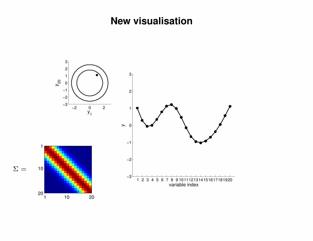
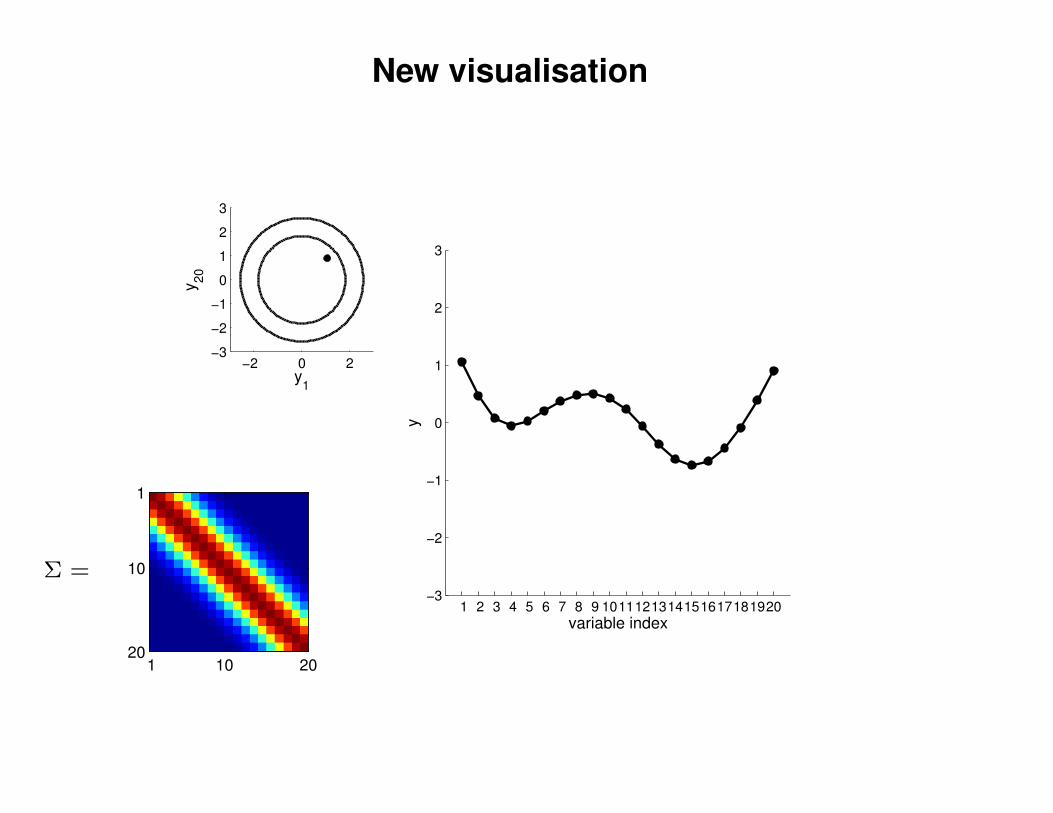
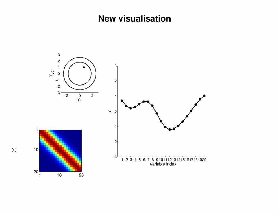
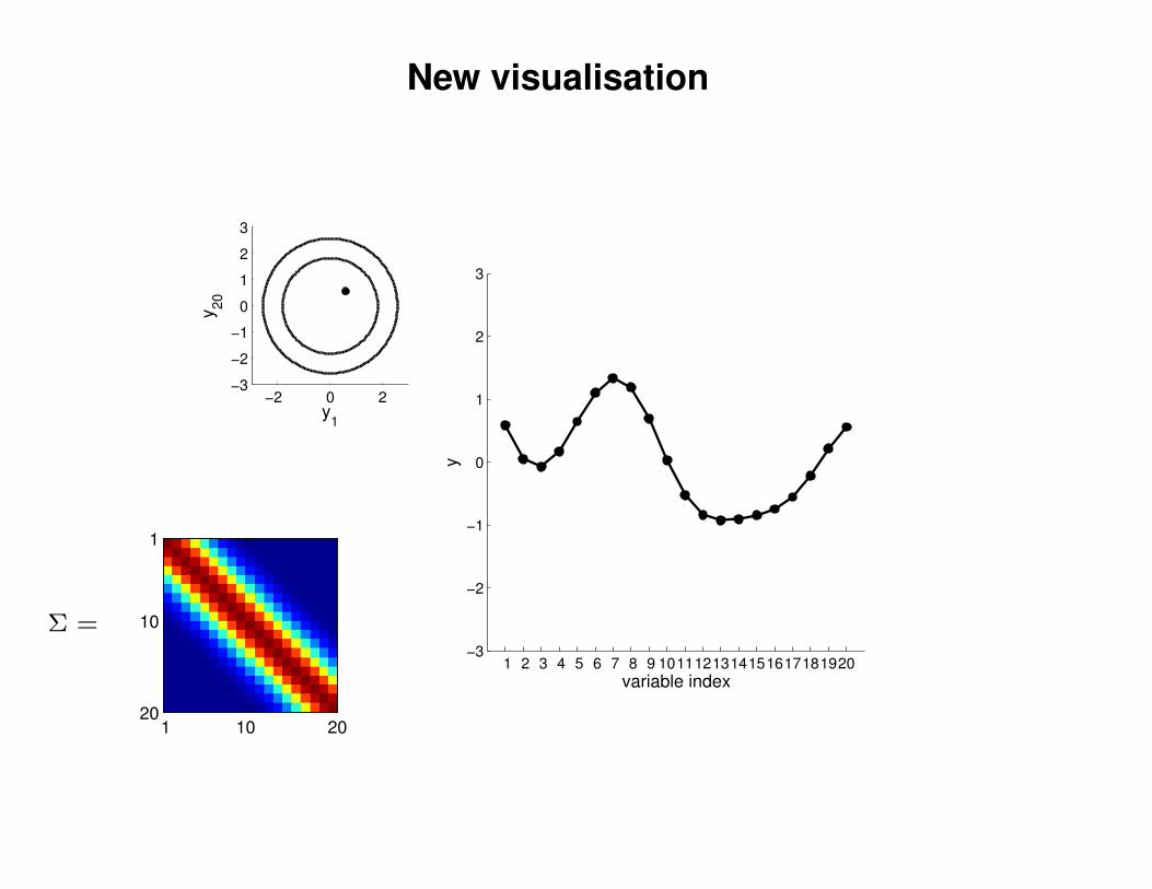
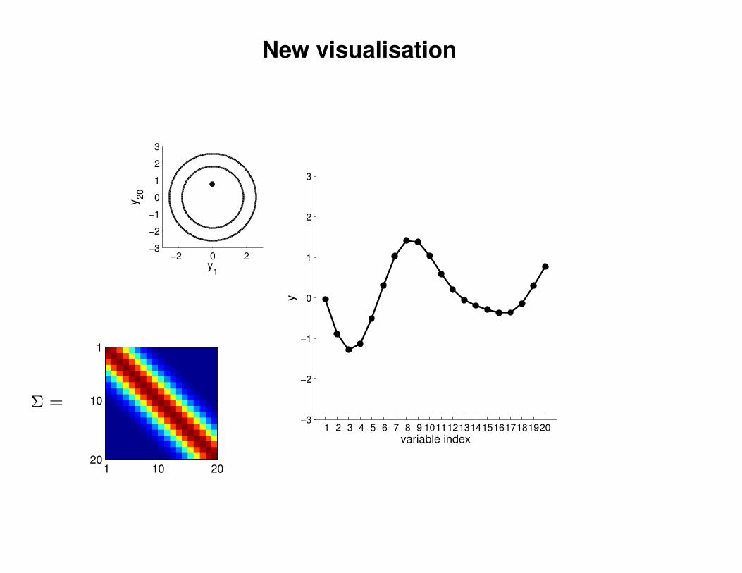
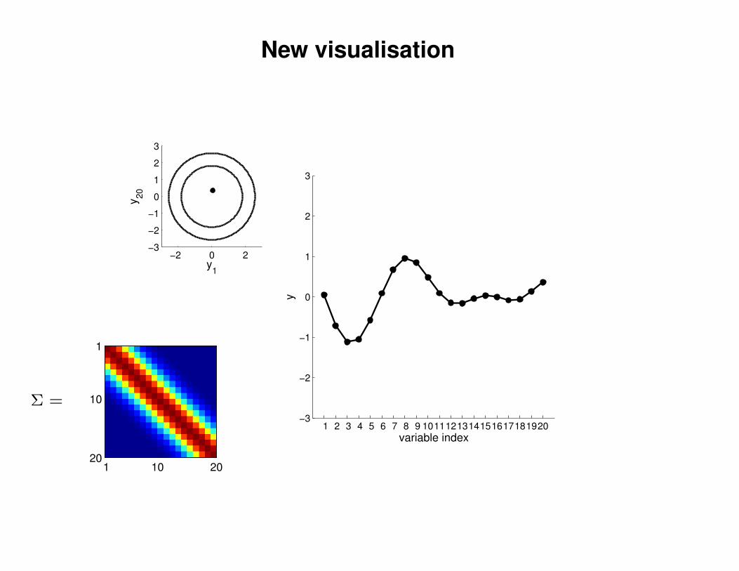
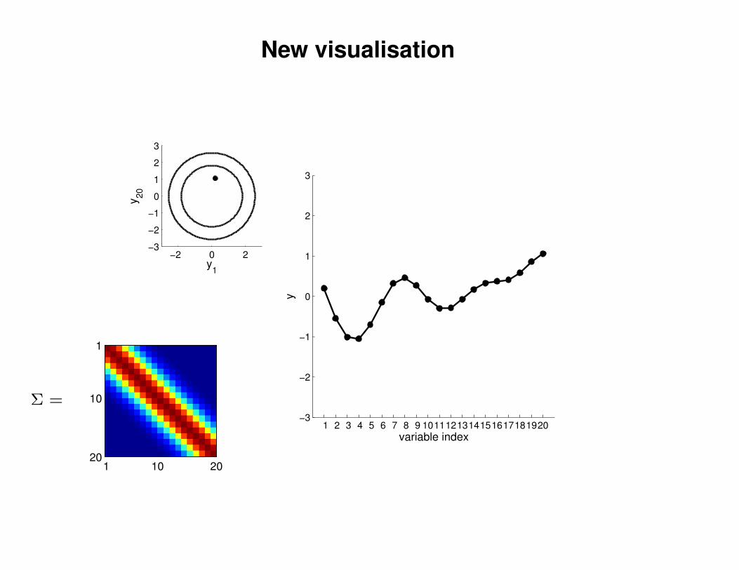
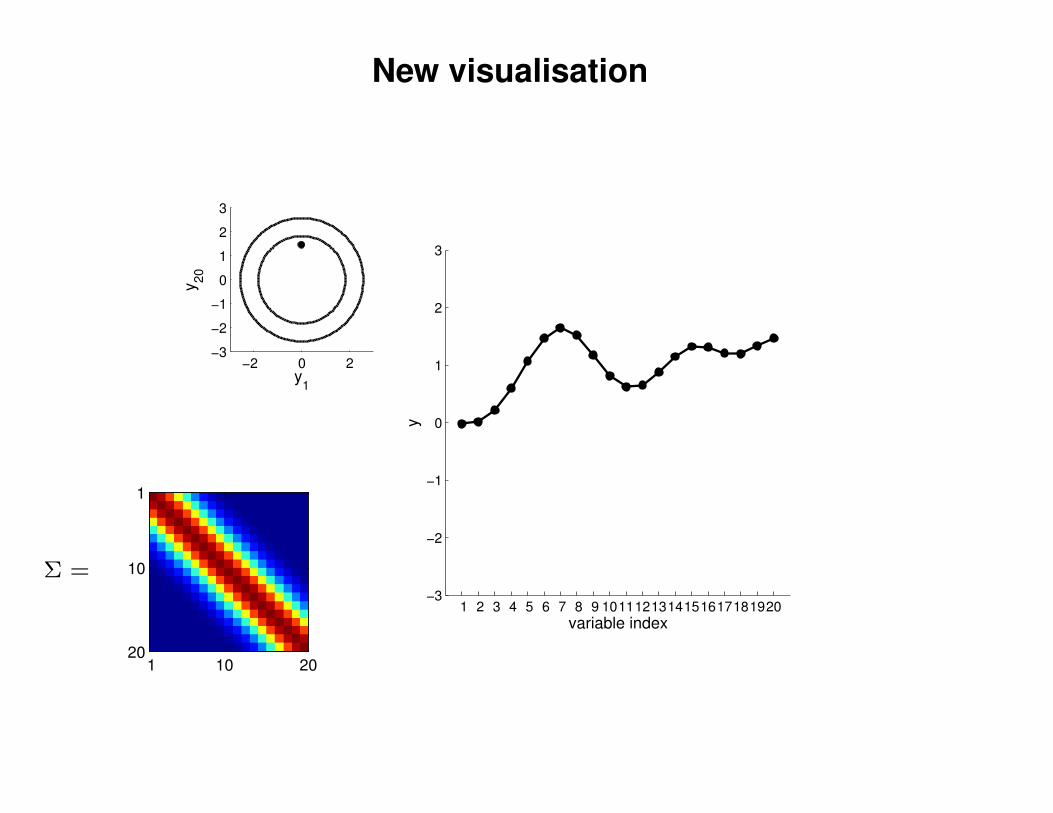
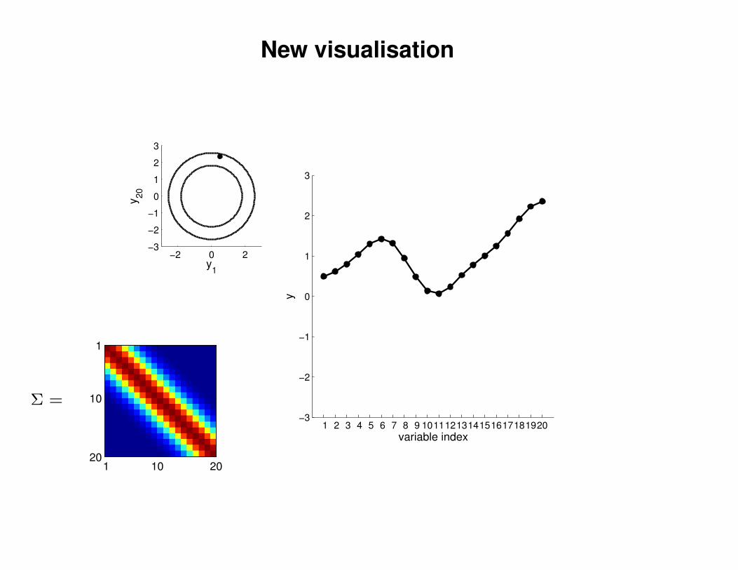
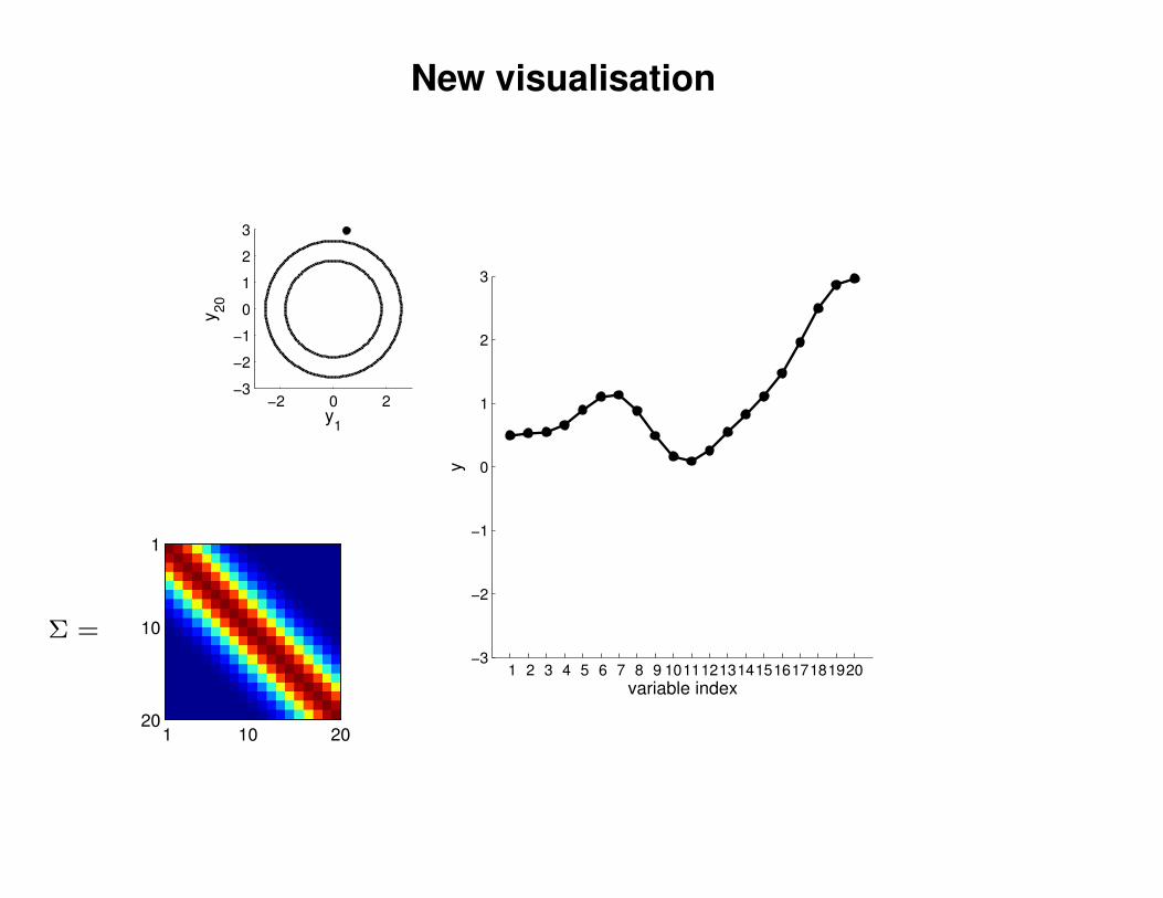
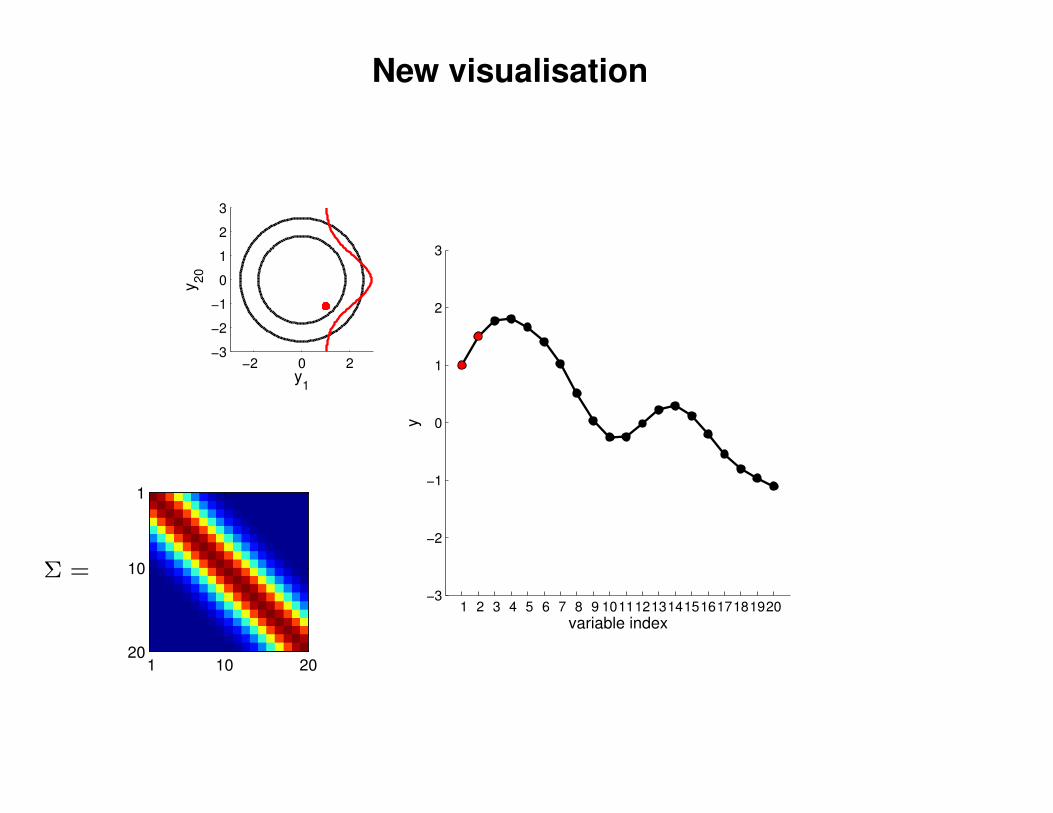
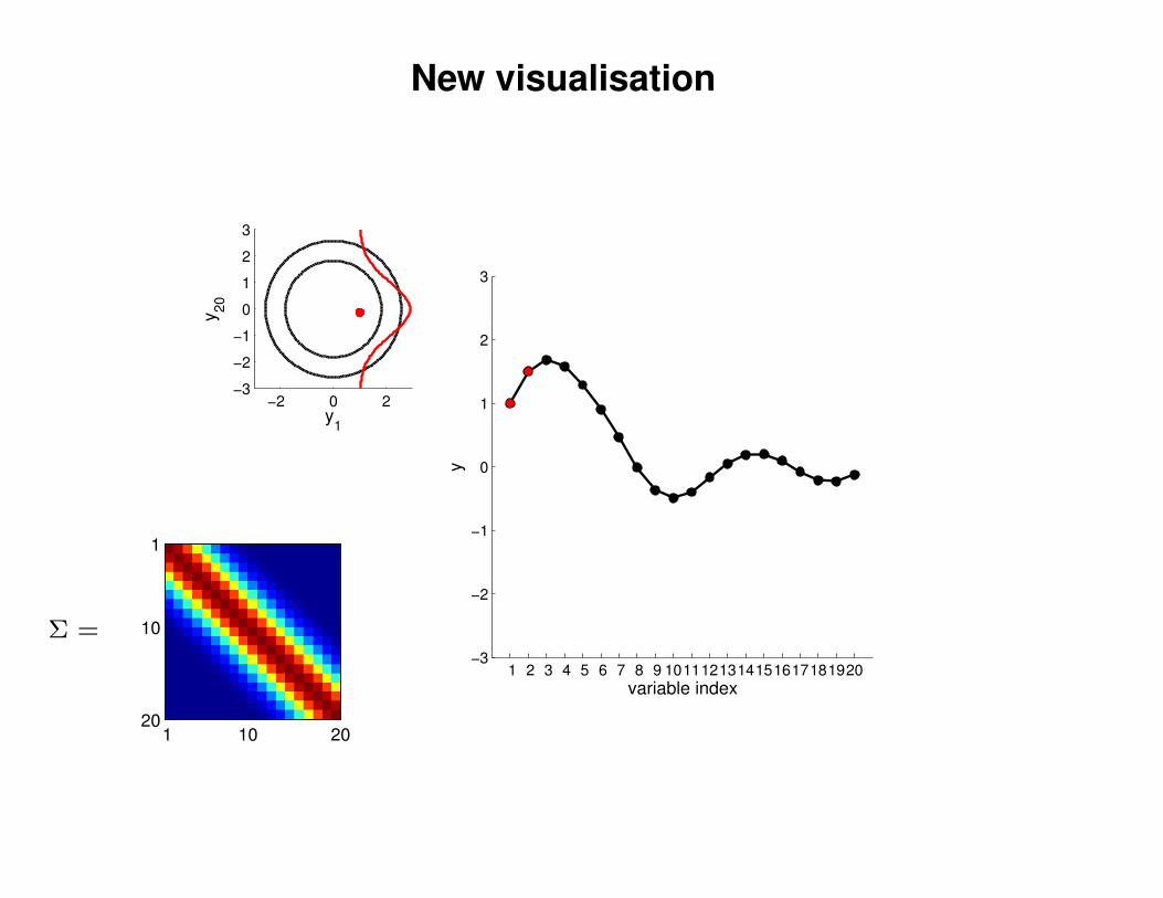
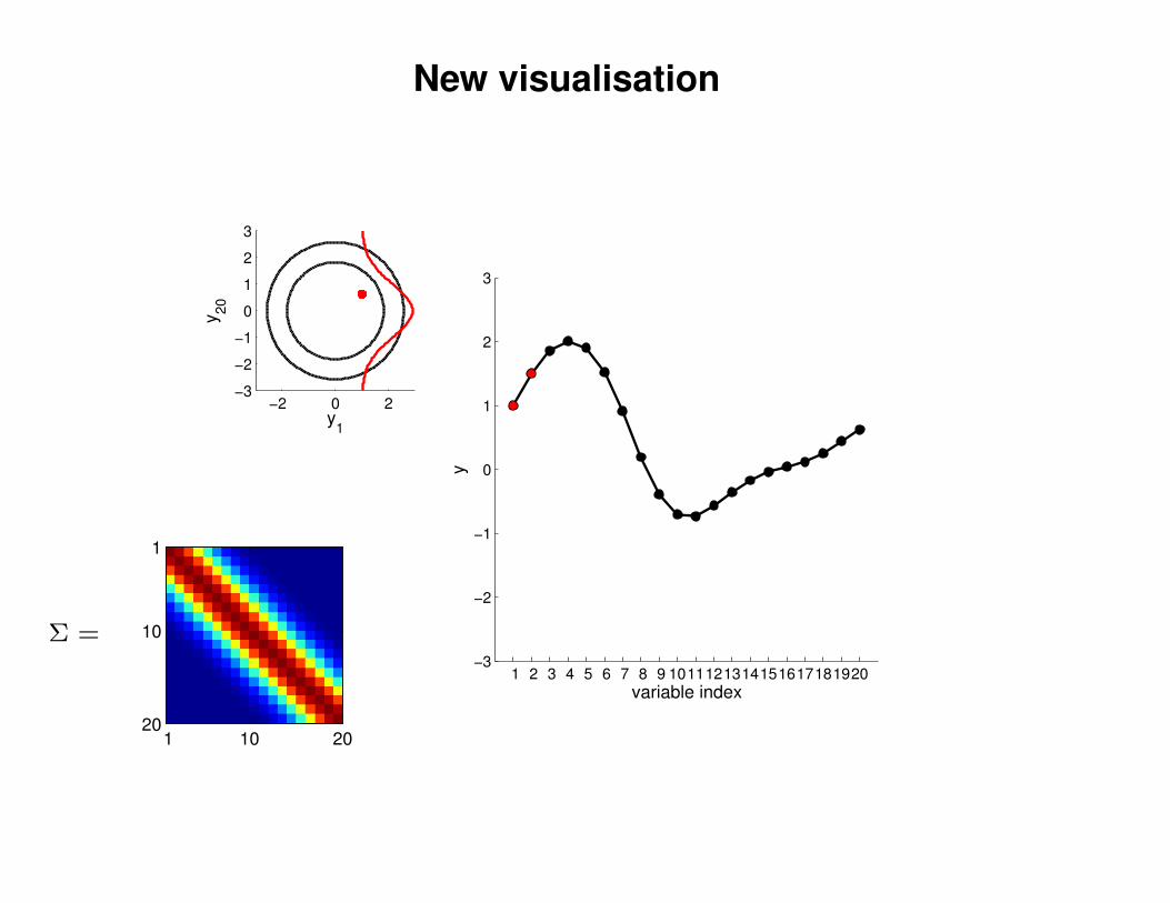
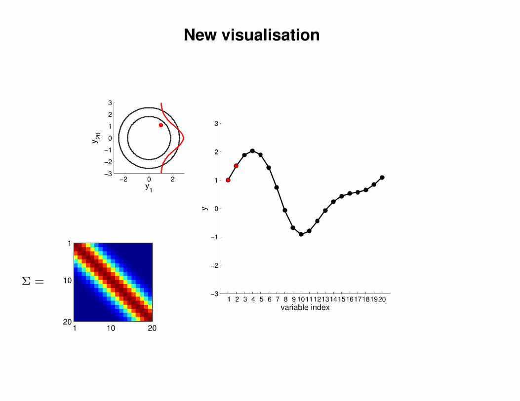
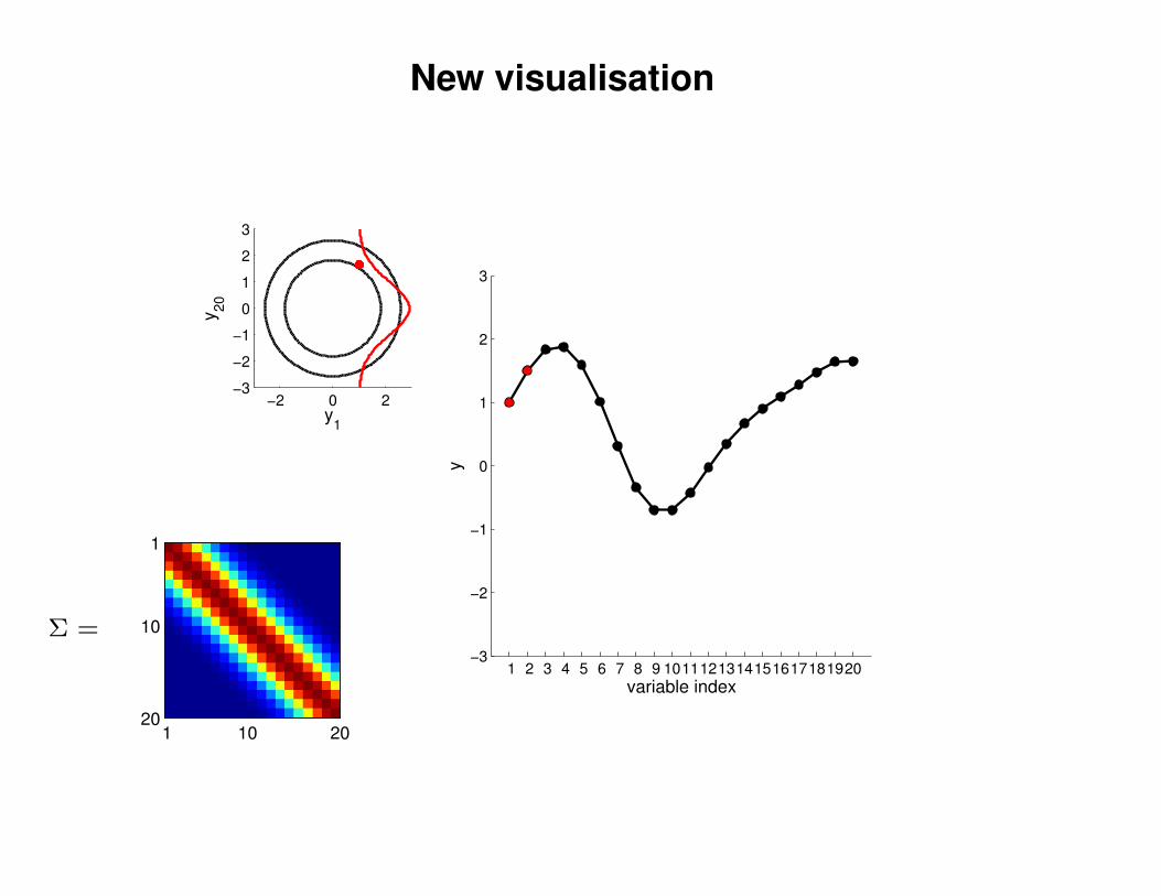
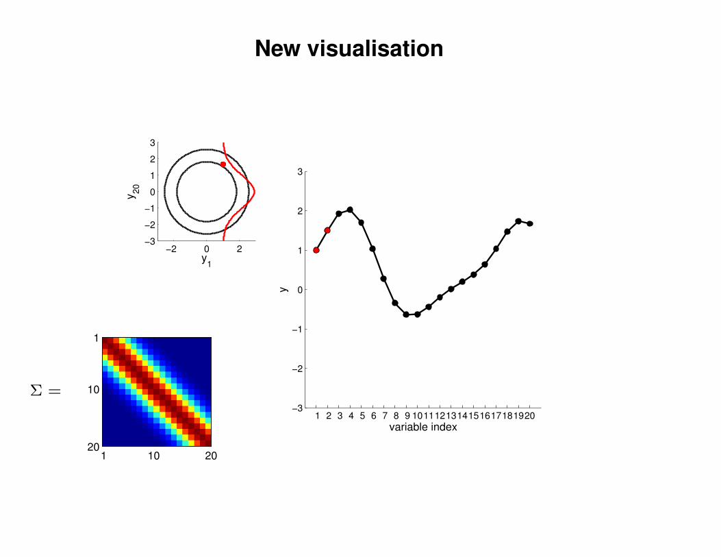
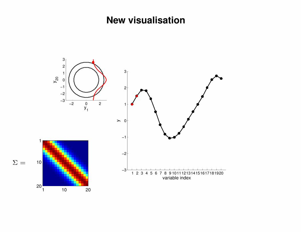
New visualisation
−2 0 2−3
−2
−1
0
1
2
3
y1
y20
1 2 3 4 5 6 7 8 9 1011121314151617181920−3
−2
−1
0
1
2
3
variable index
y
Σ =
1 10 20
1
10
20

New visualisation
−2 0 2−3
−2
−1
0
1
2
3
y1
y20
1 2 3 4 5 6 7 8 9 1011121314151617181920−3
−2
−1
0
1
2
3
variable index
y
Σ =
1 10 20
1
10
20
New visualisation
−2 0 2−3
−2
−1
0
1
2
3
y1
y20
1 2 3 4 5 6 7 8 9 1011121314151617181920−3
−2
−1
0
1
2
3
variable index
y
Σ =
1 10 20
1
10
20

New visualisation
−2 0 2−3
−2
−1
0
1
2
3
y1
y20
1 2 3 4 5 6 7 8 9 1011121314151617181920−3
−2
−1
0
1
2
3
variable index
y
Σ =
1 10 20
1
10
20
New visualisation
−2 0 2−3
−2
−1
0
1
2
3
y1
y20
1 2 3 4 5 6 7 8 9 1011121314151617181920−3
−2
−1
0
1
2
3
variable index
y
Σ =
1 10 20
1
10
20
New visualisation
−2 0 2−3
−2
−1
0
1
2
3
y1
y20
1 2 3 4 5 6 7 8 9 1011121314151617181920−3
−2
−1
0
1
2
3
variable index
y
Σ =
1 10 20
1
10
20

New visualisation
−2 0 2−3
−2
−1
0
1
2
3
y1
y20
1 2 3 4 5 6 7 8 9 1011121314151617181920−3
−2
−1
0
1
2
3
variable index
y
Σ =
1 10 20
1
10
20

New visualisation
−2 0 2−3
−2
−1
0
1
2
3
y1
y20
1 2 3 4 5 6 7 8 9 1011121314151617181920−3
−2
−1
0
1
2
3
variable index
y
Σ =
1 10 20
1
10
20
New visualisation
−2 0 2−3
−2
−1
0
1
2
3
y1
y20
1 2 3 4 5 6 7 8 9 1011121314151617181920−3
−2
−1
0
1
2
3
variable index
y
Σ =
1 10 20
1
10
20
New visualisation
−2 0 2−3
−2
−1
0
1
2
3
y1
y20
1 2 3 4 5 6 7 8 9 1011121314151617181920−3
−2
−1
0
1
2
3
variable index
y
Σ =
1 10 20
1
10
20
New visualisation
−2 0 2−3
−2
−1
0
1
2
3
y1
y20
1 2 3 4 5 6 7 8 9 1011121314151617181920−3
−2
−1
0
1
2
3
variable index
y
Σ =
1 10 20
1
10
20

New visualisation
−2 0 2−3
−2
−1
0
1
2
3
y1
y20
1 2 3 4 5 6 7 8 9 1011121314151617181920−3
−2
−1
0
1
2
3
variable index
y
Σ =
1 10 20
1
10
20

New visualisation
−2 0 2−3
−2
−1
0
1
2
3
y1
y20
1 2 3 4 5 6 7 8 9 1011121314151617181920−3
−2
−1
0
1
2
3
variable index
y
Σ =
1 10 20
1
10
20

New visualisation
−2 0 2−3
−2
−1
0
1
2
3
y1
y20
1 2 3 4 5 6 7 8 9 1011121314151617181920−3
−2
−1
0
1
2
3
variable index
y
Σ =
1 10 20
1
10
20

New visualisation
−2 0 2−3
−2
−1
0
1
2
3
y1
y20
1 2 3 4 5 6 7 8 9 1011121314151617181920−3
−2
−1
0
1
2
3
variable index
y
Σ =
1 10 20
1
10
20
New visualisation
−2 0 2−3
−2
−1
0
1
2
3
y1
y20
1 2 3 4 5 6 7 8 9 1011121314151617181920−3
−2
−1
0
1
2
3
variable index
y
Σ =
1 10 20
1
10
20

New visualisation
−2 0 2−3
−2
−1
0
1
2
3
y1
y20
1 2 3 4 5 6 7 8 9 1011121314151617181920−3
−2
−1
0
1
2
3
variable index
y
Σ =
1 10 20
1
10
20

New visualisation
−2 0 2−3
−2
−1
0
1
2
3
y1
y20
1 2 3 4 5 6 7 8 9 1011121314151617181920−3
−2
−1
0
1
2
3
variable index
y
Σ =
1 10 20
1
10
20
New visualisation
−2 0 2−3
−2
−1
0
1
2
3
y1
y20
1 2 3 4 5 6 7 8 9 1011121314151617181920−3
−2
−1
0
1
2
3
variable index
y
Σ =
1 10 20
1
10
20
New visualisation
−2 0 2−3
−2
−1
0
1
2
3
y1
y20
1 2 3 4 5 6 7 8 9 1011121314151617181920−3
−2
−1
0
1
2
3
variable index
y
Σ =
1 10 20
1
10
20

New visualisation
−2 0 2−3
−2
−1
0
1
2
3
y1
y20
1 2 3 4 5 6 7 8 9 1011121314151617181920−3
−2
−1
0
1
2
3
variable index
y
Σ =
1 10 20
1
10
20

New visualisation
−2 0 2−3
−2
−1
0
1
2
3
y1
y20
1 2 3 4 5 6 7 8 9 1011121314151617181920−3
−2
−1
0
1
2
3
variable index
y
Σ =
1 10 20
1
10
20

New visualisation
−2 0 2−3
−2
−1
0
1
2
3
y1
y20
1 2 3 4 5 6 7 8 9 1011121314151617181920−3
−2
−1
0
1
2
3
variable index
y
Σ =
1 10 20
1
10
20

New visualisation
−2 0 2−3
−2
−1
0
1
2
3
y1
y20
1 2 3 4 5 6 7 8 9 1011121314151617181920−3
−2
−1
0
1
2
3
variable index
y
Σ =
1 10 20
1
10
20

New visualisation
−2 0 2−3
−2
−1
0
1
2
3
y1
y20
1 2 3 4 5 6 7 8 9 1011121314151617181920−3
−2
−1
0
1
2
3
variable index
y
Σ =
1 10 20
1
10
20

New visualisation
−2 0 2−3
−2
−1
0
1
2
3
y1
y20
1 2 3 4 5 6 7 8 9 1011121314151617181920−3
−2
−1
0
1
2
3
variable index
y
Σ =
1 10 20
1
10
20

New visualisation
−2 0 2−3
−2
−1
0
1
2
3
y1
y20
1 2 3 4 5 6 7 8 9 1011121314151617181920−3
−2
−1
0
1
2
3
variable index
y
Σ =
1 10 20
1
10
20

New visualisation
−2 0 2−3
−2
−1
0
1
2
3
y1
y20
1 2 3 4 5 6 7 8 9 1011121314151617181920−3
−2
−1
0
1
2
3
variable index
y
Σ =
1 10 20
1
10
20

New visualisation
−2 0 2−3
−2
−1
0
1
2
3
y1
y20
1 2 3 4 5 6 7 8 9 1011121314151617181920−3
−2
−1
0
1
2
3
variable index
y
Σ =
1 10 20
1
10
20

New visualisation
−2 0 2−3
−2
−1
0
1
2
3
y1
y20
1 2 3 4 5 6 7 8 9 1011121314151617181920−3
−2
−1
0
1
2
3
variable index
y
Σ =
1 10 20
1
10
20
New visualisation
−2 0 2−3
−2
−1
0
1
2
3
y1
y20
1 2 3 4 5 6 7 8 9 1011121314151617181920−3
−2
−1
0
1
2
3
variable index
y
Σ =
1 10 20
1
10
20

New visualisation
−2 0 2−3
−2
−1
0
1
2
3
y1
y20
1 2 3 4 5 6 7 8 9 1011121314151617181920−3
−2
−1
0
1
2
3
variable index
y
Σ =
1 10 20
1
10
20

New visualisation
−2 0 2−3
−2
−1
0
1
2
3
y1
y20
1 2 3 4 5 6 7 8 9 1011121314151617181920−3
−2
−1
0
1
2
3
variable index
y
Σ =
1 10 20
1
10
20
New visualisation
−2 0 2−3
−2
−1
0
1
2
3
y1
y20
1 2 3 4 5 6 7 8 9 1011121314151617181920−3
−2
−1
0
1
2
3
variable index
y
Σ =
1 10 20
1
10
20
New visualisation
−2 0 2−3
−2
−1
0
1
2
3
y1
y20
1 2 3 4 5 6 7 8 9 1011121314151617181920−3
−2
−1
0
1
2
3
variable index
y
Σ =
1 10 20
1
10
20
New visualisation
−2 0 2−3
−2
−1
0
1
2
3
y1
y20
1 2 3 4 5 6 7 8 9 1011121314151617181920−3
−2
−1
0
1
2
3
variable index
y
Σ =
1 10 20
1
10
20
New visualisation
−2 0 2−3
−2
−1
0
1
2
3
y1
y20
1 2 3 4 5 6 7 8 9 1011121314151617181920−3
−2
−1
0
1
2
3
variable index
y
Σ =
1 10 20
1
10
20
New visualisation
−2 0 2−3
−2
−1
0
1
2
3
y1
y20
1 2 3 4 5 6 7 8 9 1011121314151617181920−3
−2
−1
0
1
2
3
variable index
y
Σ =
1 10 20
1
10
20
New visualisation
−2 0 2−3
−2
−1
0
1
2
3
y1
y20
1 2 3 4 5 6 7 8 9 1011121314151617181920−3
−2
−1
0
1
2
3
variable index
y
Σ =
1 10 20
1
10
20

New visualisation
−2 0 2−3
−2
−1
0
1
2
3
y1
y20
1 2 3 4 5 6 7 8 9 1011121314151617181920−3
−2
−1
0
1
2
3
variable index
y
Σ =
1 10 20
1
10
20
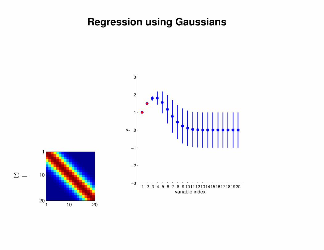
Regression using Gaussians
1 2 3 4 5 6 7 8 9 1011121314151617181920−3
−2
−1
0
1
2
3
variable index
y
Σ =
1 10 20
1
10
20
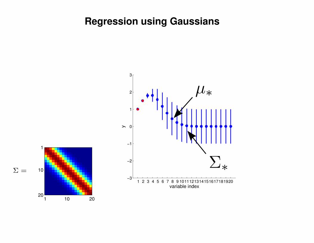
Regression using Gaussians
1 2 3 4 5 6 7 8 9 1011121314151617181920−3
−2
−1
0
1
2
3
variable index
y
Σ =
1 10 20
1
10
20
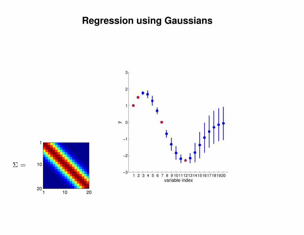
Regression using Gaussians
1 2 3 4 5 6 7 8 9 1011121314151617181920−3
−2
−1
0
1
2
3
variable index
y
Σ =
1 10 20
1
10
20

Regression using Gaussians
1 2 3 4 5 6 7 8 9 1011121314151617181920−3
−2
−1
0
1
2
3
variable index
y
Σ =
Σ(x1, x2) = K(x1, x2) + Iσ2y
K(x1, x2) = σ2 exp(− 1
2l2(x1 − x2)2
)
1 10 20
1
10
20
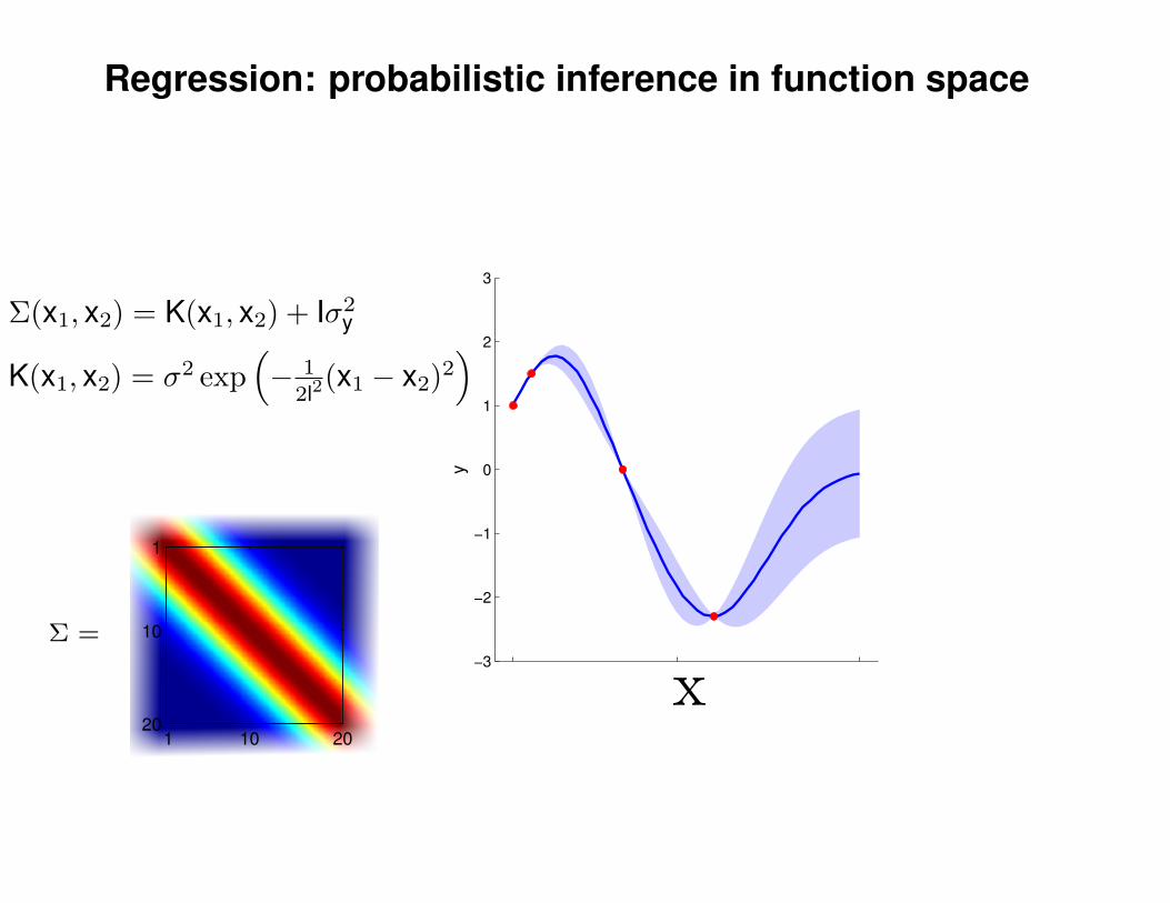
Regression: probabilistic inference in function space
−3
−2
−1
0
1
2
3
y
Σ =
Σ(x1, x2) = K(x1, x2) + Iσ2y
K(x1, x2) = σ2 exp(− 1
2l2(x1 − x2)2
)
1 10 20
1
10
20
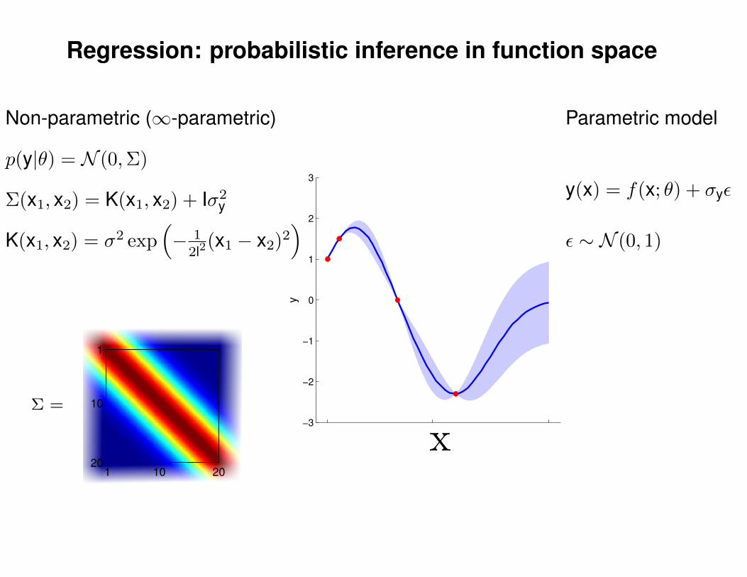
Regression: probabilistic inference in function space
−3
−2
−1
0
1
2
3
y
Σ =
Σ(x1, x2) = K(x1, x2) + Iσ2y
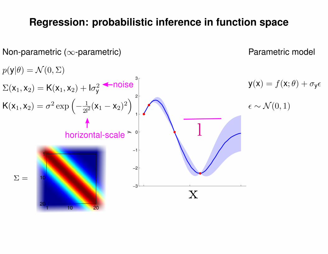
p(y|θ) = N (0,Σ)
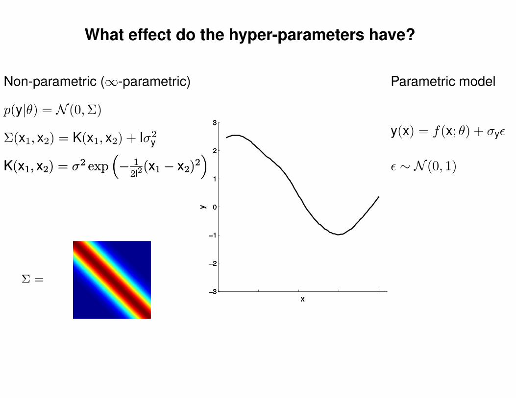
Non-parametric (∞-parametric)
K(x1, x2) = σ2 exp(− 1
2l2(x1 − x2)2
)
1 10 20
1
10
20
Parametric model
y(x) = f(x; θ) + σyε
ε ∼ N (0, 1)
Regression: probabilistic inference in function space
−3
−2
−1
0
1
2
3
y
Σ =
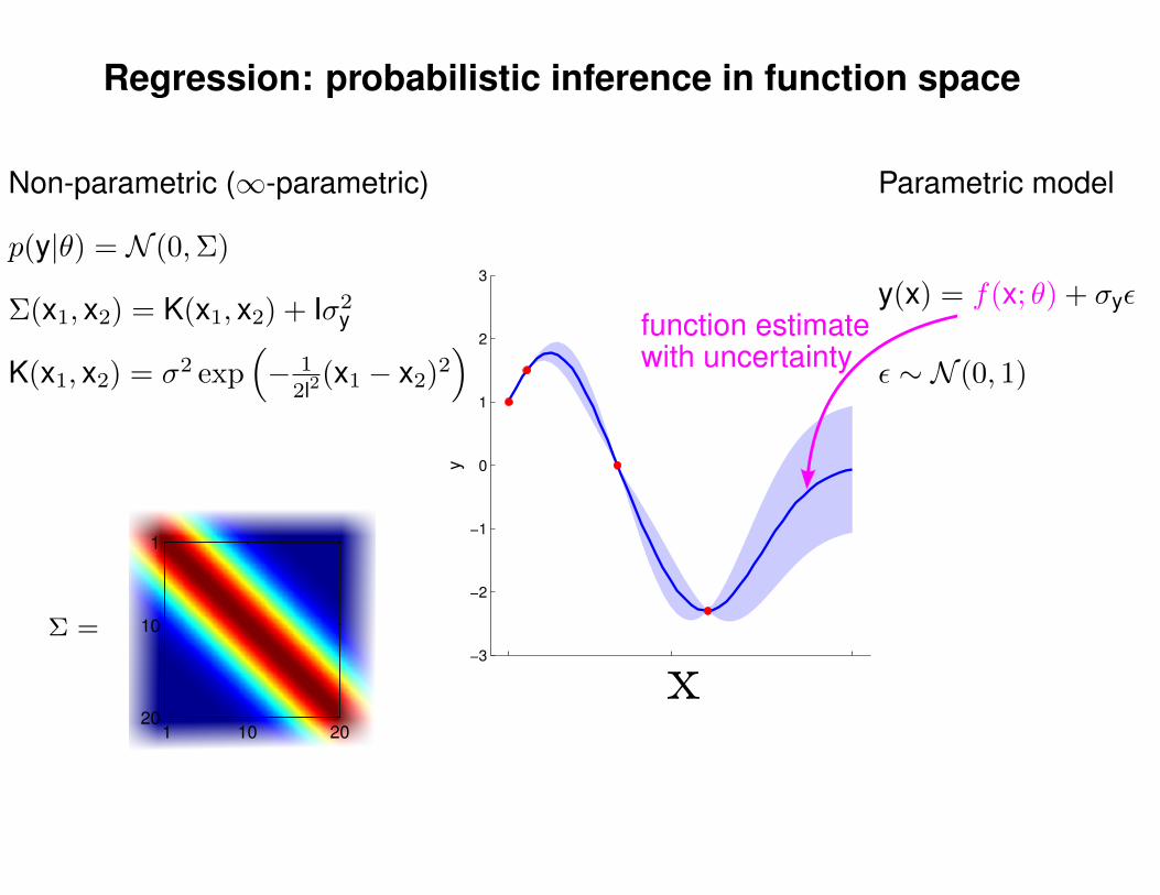
Σ(x1, x2) = K(x1, x2) + Iσ2y
Non-parametric (∞-parametric)
p(y|θ) = N (0,Σ)
function estimatewith uncertaintyK(x1, x2) = σ2 exp
(− 1
2l2(x1 − x2)2
)
1 10 20
1
10
20
Parametric model
y(x) = f(x; θ) + σyε
ε ∼ N (0, 1)
Regression: probabilistic inference in function space
−3
−2
−1
0
1
2
3
y
Σ =
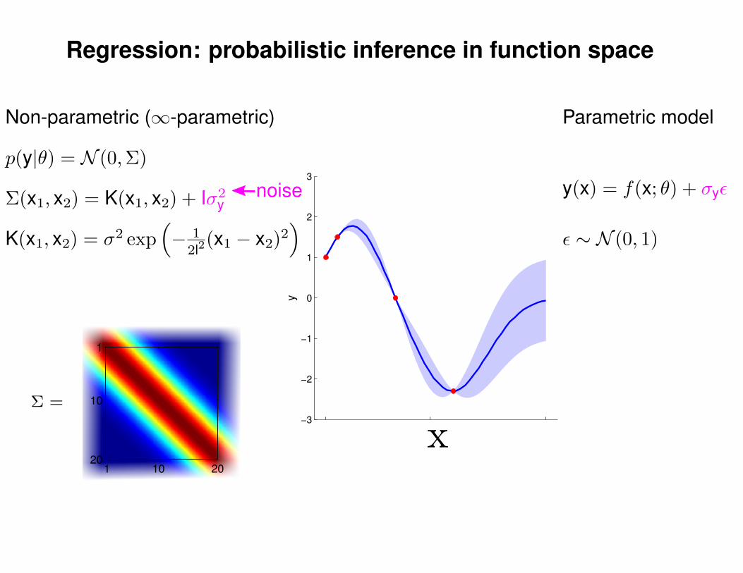
Σ(x1, x2) = K(x1, x2) + Iσ2y
p(y|θ) = N (0,Σ)
Non-parametric (∞-parametric)
noise
K(x1, x2) = σ2 exp(− 1
2l2(x1 − x2)2
)
1 10 20
1
10
20
Parametric model
y(x) = f(x; θ) + σyε
ε ∼ N (0, 1)
Regression: probabilistic inference in function space
−3
−2
−1
0
1
2
3
y
Σ =
Σ(x1, x2) = K(x1, x2) + Iσ2y
p(y|θ) = N (0,Σ)
Non-parametric (∞-parametric)
horizontal-scale
noise
K(x1, x2) = σ2 exp(− 1
2l2(x1 − x2)2
)
1 10 20
1
10
20
Parametric model
y(x) = f(x; θ) + σyε
ε ∼ N (0, 1)
Regression: probabilistic inference in function space
−3
−2
−1
0
1
2
3
y
Σ =
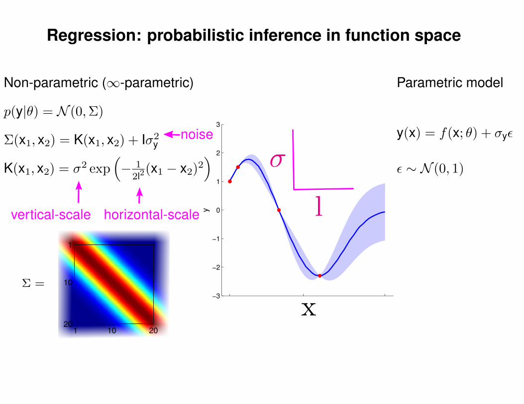
Σ(x1, x2) = K(x1, x2) + Iσ2y
p(y|θ) = N (0,Σ)
Non-parametric (∞-parametric)
noise
Parametric model
y(x) = f(x; θ) + σyε
ε ∼ N (0, 1)K(x1, x2) = σ2 exp(− 1
2l2(x1 − x2)2
)
1 10 20
1
10
20
horizontal-scalevertical-scale
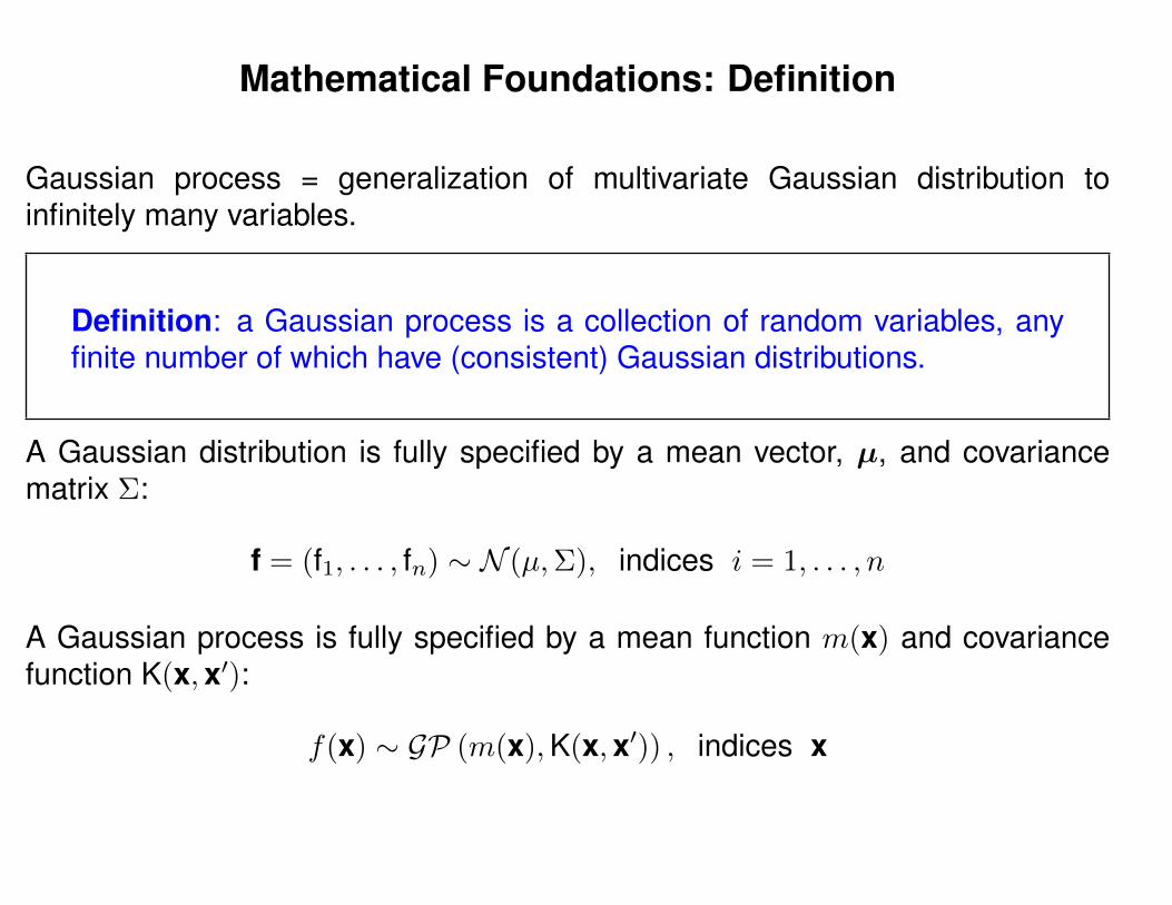
Mathematical Foundations: Definition
Gaussian process = generalization of multivariate Gaussian distribution toinfinitely many variables.
Definition: a Gaussian process is a collection of random variables, anyfinite number of which have (consistent) Gaussian distributions.
A Gaussian distribution is fully specified by a mean vector, µ, and covariancematrix Σ:
f = (f1, . . . , fn) ∼ N (µ,Σ), indices i = 1, . . . , n
A Gaussian process is fully specified by a mean function m(x) and covariancefunction K(x,x′):
f(x) ∼ GP (m(x),K(x,x′)) , indices x
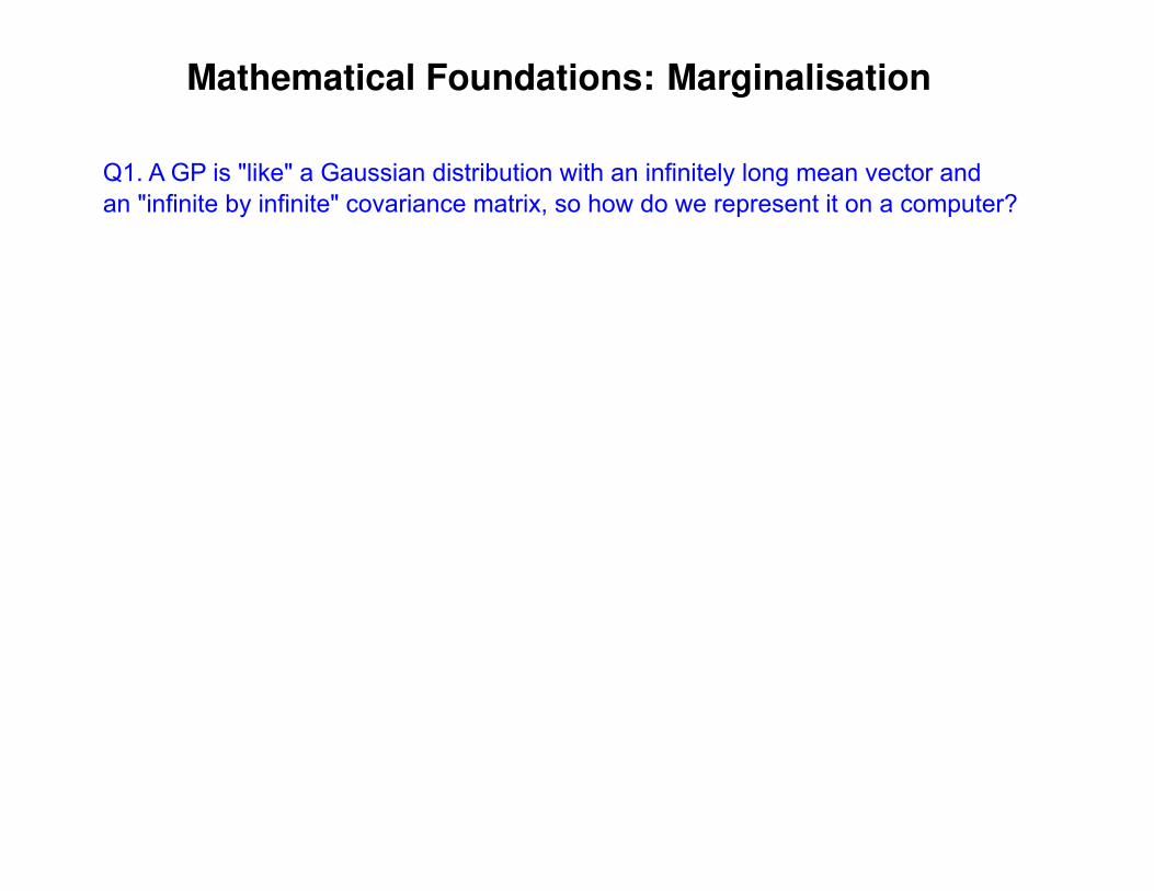
Mathematical Foundations: Marginalisation
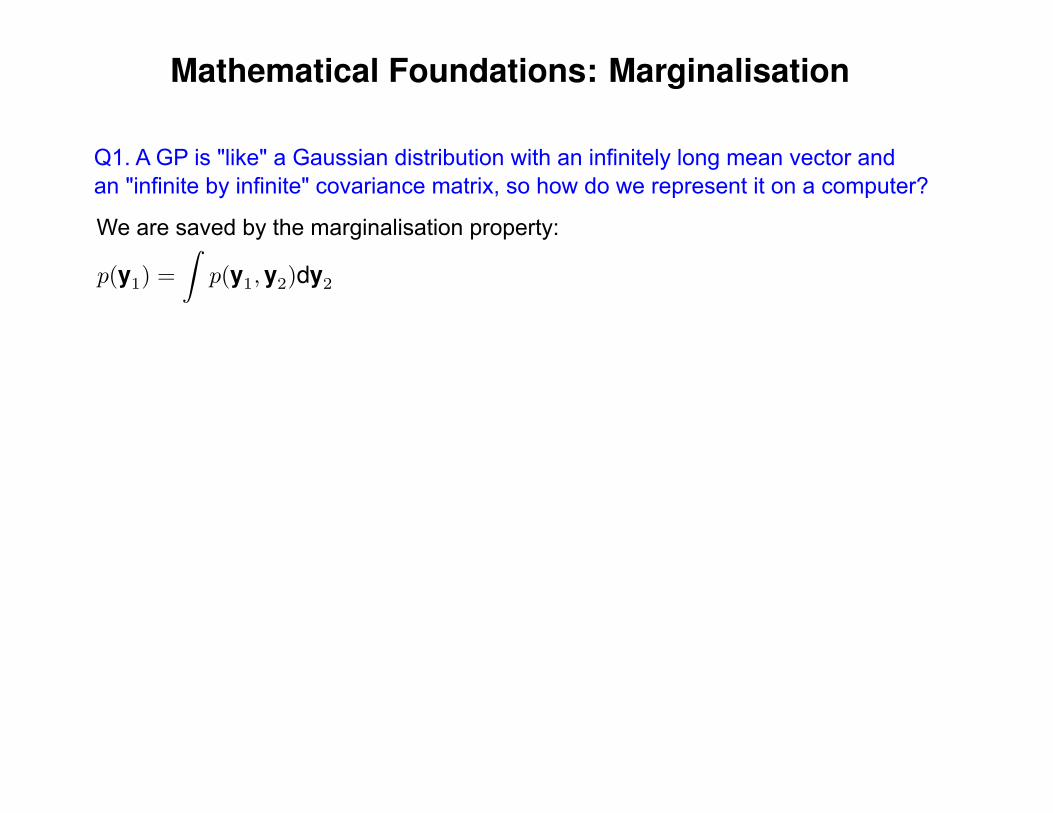
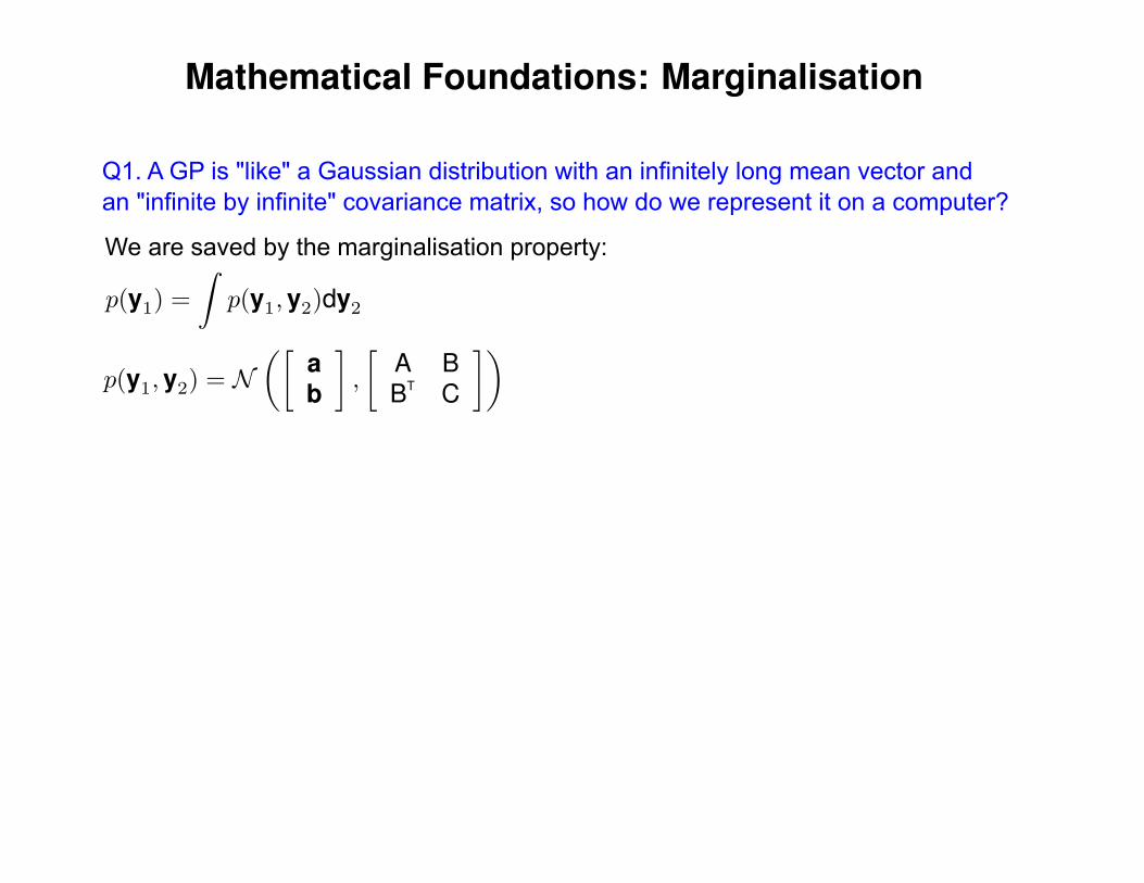
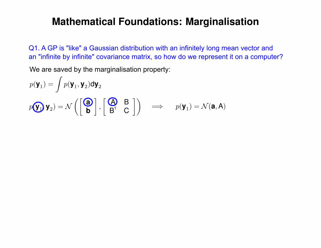
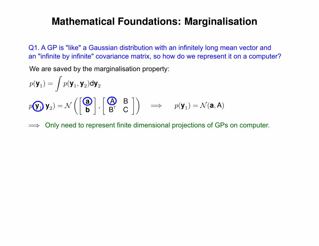
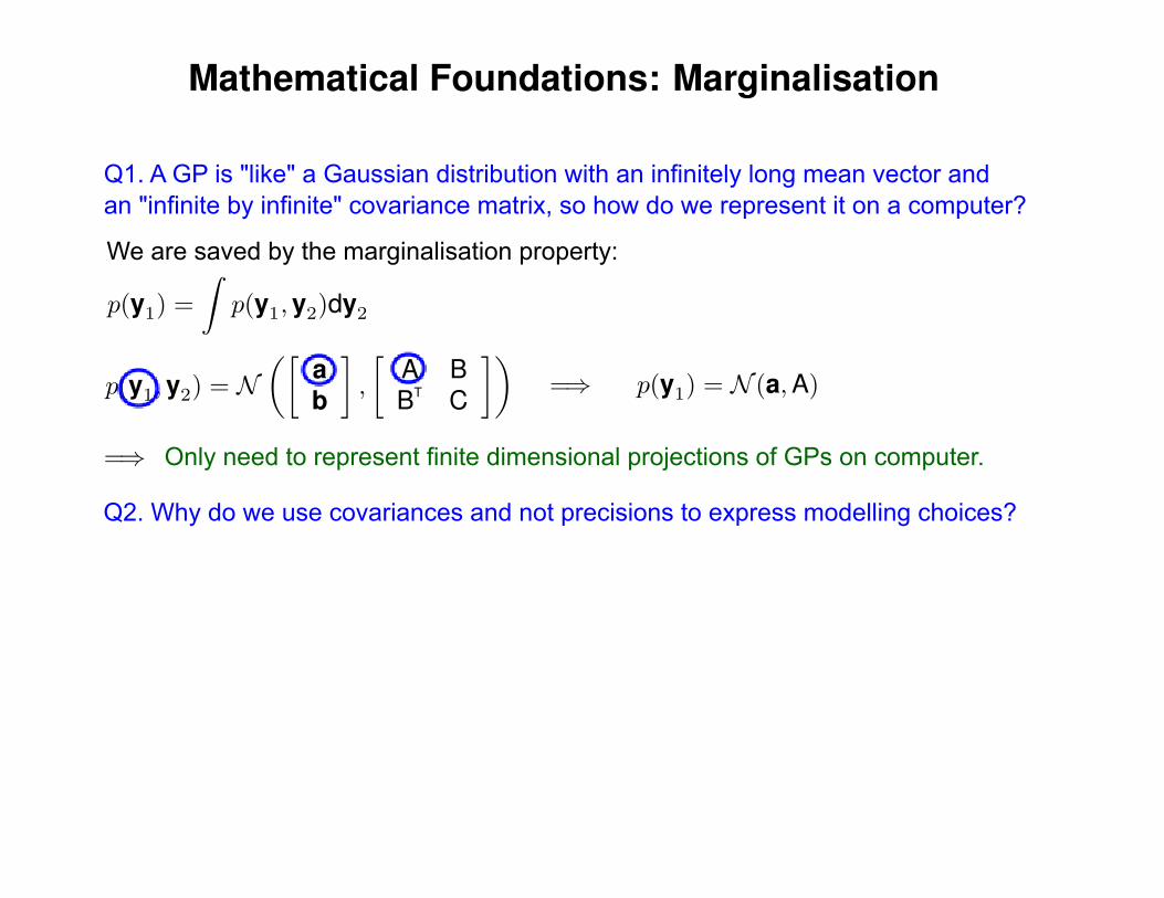
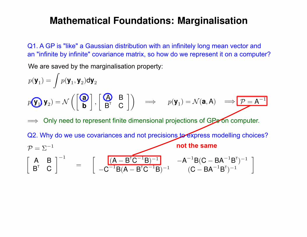
Q1. A GP is "like" a Gaussian distribution with an infinitely long mean vector and an "infinite by infinite" covariance matrix, so how do we represent it on a computer?
Mathematical Foundations: Marginalisation
Q1. A GP is "like" a Gaussian distribution with an infinitely long mean vector and an "infinite by infinite" covariance matrix, so how do we represent it on a computer?
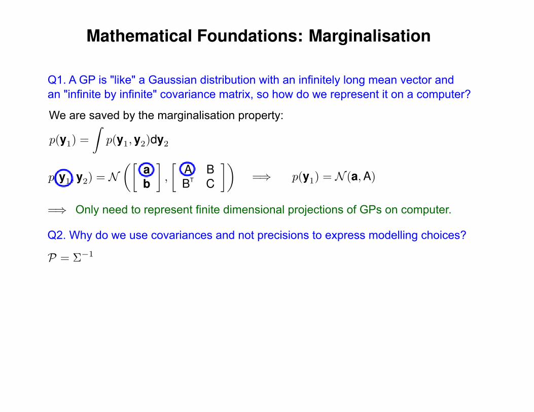
We are saved by the marginalisation property:
Mathematical Foundations: Marginalisation
Q1. A GP is "like" a Gaussian distribution with an infinitely long mean vector and an "infinite by infinite" covariance matrix, so how do we represent it on a computer?
We are saved by the marginalisation property:

Mathematical Foundations: Marginalisation
Q1. A GP is "like" a Gaussian distribution with an infinitely long mean vector and an "infinite by infinite" covariance matrix, so how do we represent it on a computer?
We are saved by the marginalisation property:
Mathematical Foundations: Marginalisation
Q1. A GP is "like" a Gaussian distribution with an infinitely long mean vector and an "infinite by infinite" covariance matrix, so how do we represent it on a computer?
We are saved by the marginalisation property:
Mathematical Foundations: Marginalisation
Q1. A GP is "like" a Gaussian distribution with an infinitely long mean vector and an "infinite by infinite" covariance matrix, so how do we represent it on a computer?
We are saved by the marginalisation property:
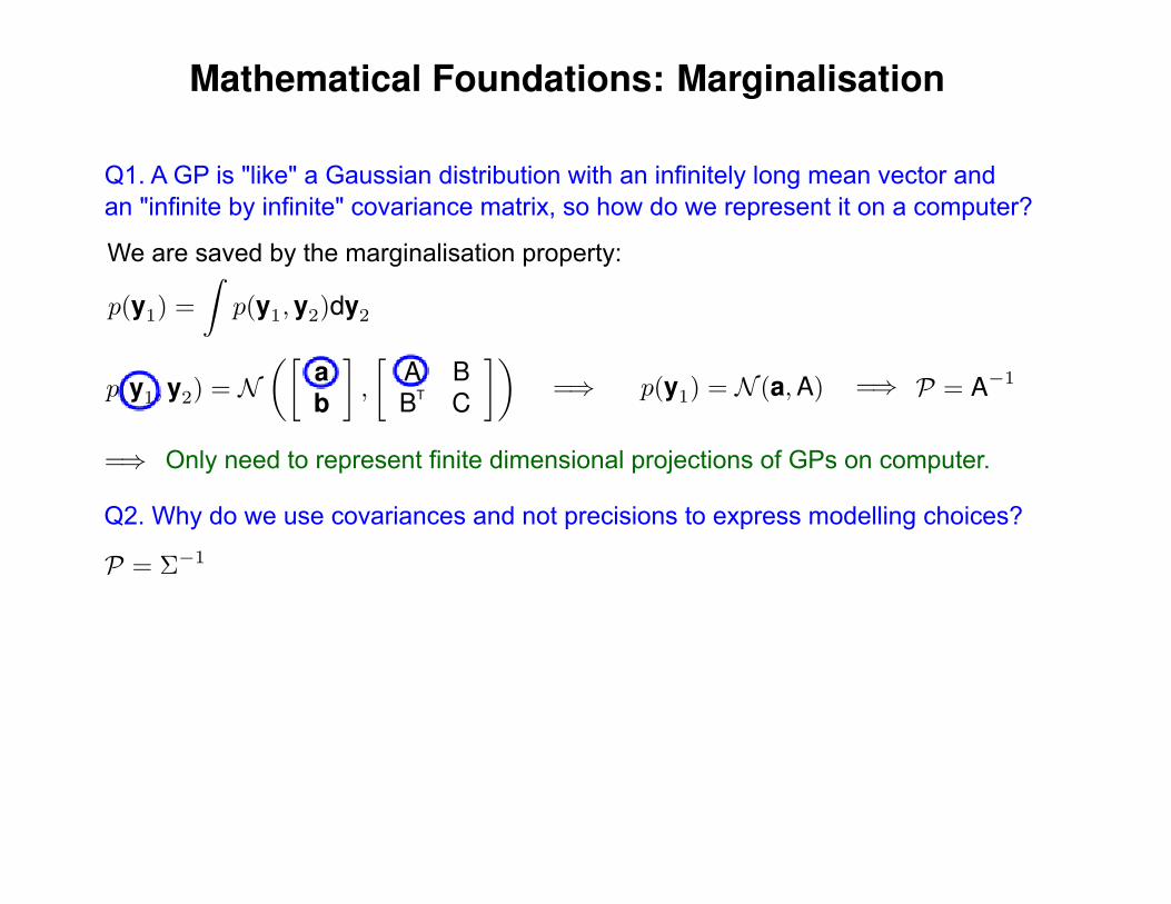
Only need to represent finite dimensional projections of GPs on computer.
Mathematical Foundations: Marginalisation
Q1. A GP is "like" a Gaussian distribution with an infinitely long mean vector and an "infinite by infinite" covariance matrix, so how do we represent it on a computer?
We are saved by the marginalisation property:
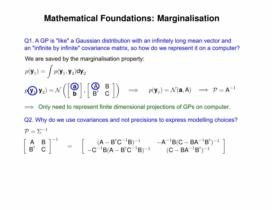
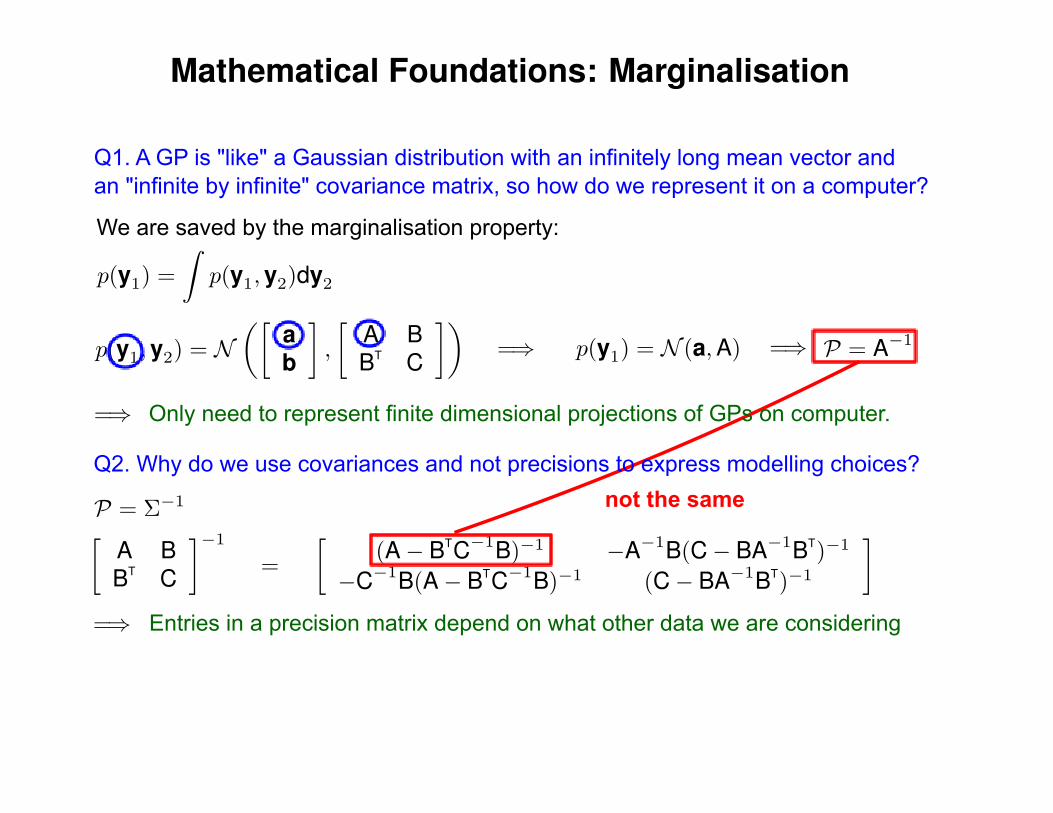
Q2. Why do we use covariances and not precisions to express modelling choices?
Only need to represent finite dimensional projections of GPs on computer.
Mathematical Foundations: Marginalisation
Q1. A GP is "like" a Gaussian distribution with an infinitely long mean vector and an "infinite by infinite" covariance matrix, so how do we represent it on a computer?
We are saved by the marginalisation property:
Q2. Why do we use covariances and not precisions to express modelling choices?
Only need to represent finite dimensional projections of GPs on computer.
not the same
Mathematical Foundations: Marginalisation
Q1. A GP is "like" a Gaussian distribution with an infinitely long mean vector and an "infinite by infinite" covariance matrix, so how do we represent it on a computer?
We are saved by the marginalisation property:
Q2. Why do we use covariances and not precisions to express modelling choices?
Only need to represent finite dimensional projections of GPs on computer.
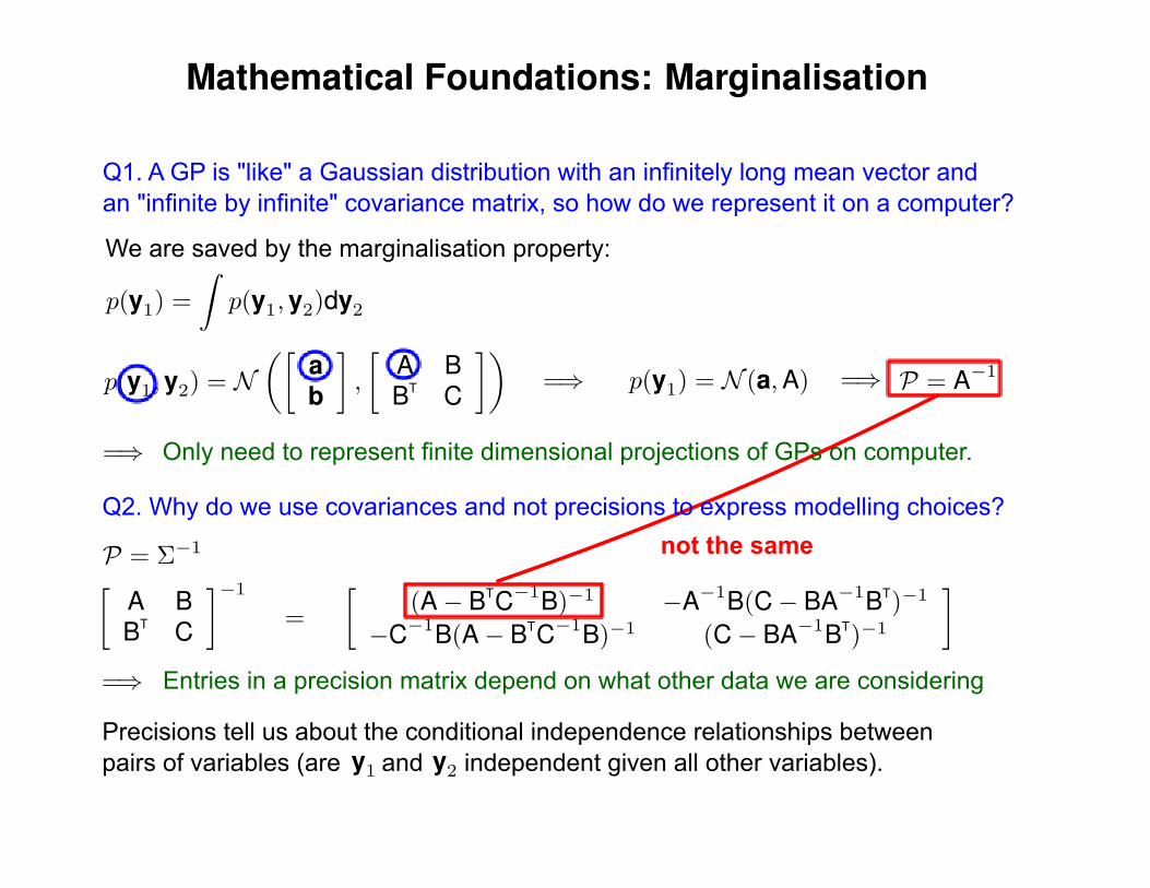
Entries in a precision matrix depend on what other data we are considering
not the same
Mathematical Foundations: Marginalisation
Q1. A GP is "like" a Gaussian distribution with an infinitely long mean vector and an "infinite by infinite" covariance matrix, so how do we represent it on a computer?
We are saved by the marginalisation property:
Q2. Why do we use covariances and not precisions to express modelling choices?
Only need to represent finite dimensional projections of GPs on computer.
Precisions tell us about the conditional independence relationships betweenpairs of variables (are and independent given all other variables).
Entries in a precision matrix depend on what other data we are considering
not the same
Mathematical Foundations: Regression
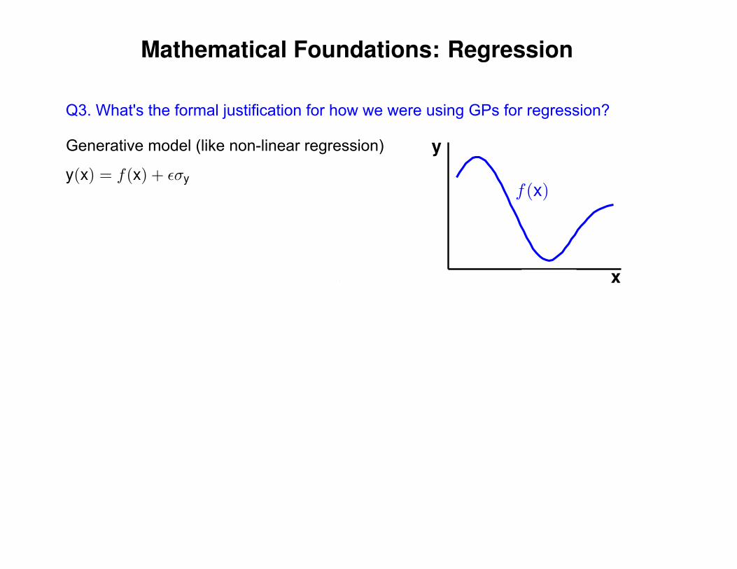
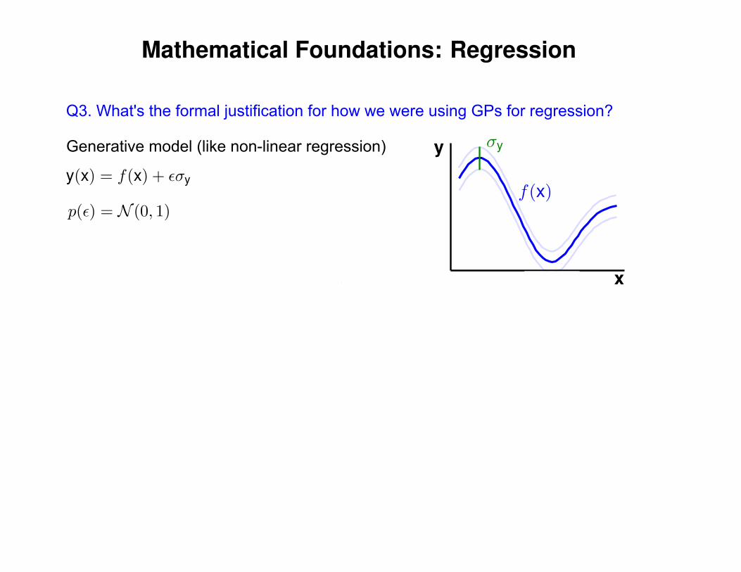
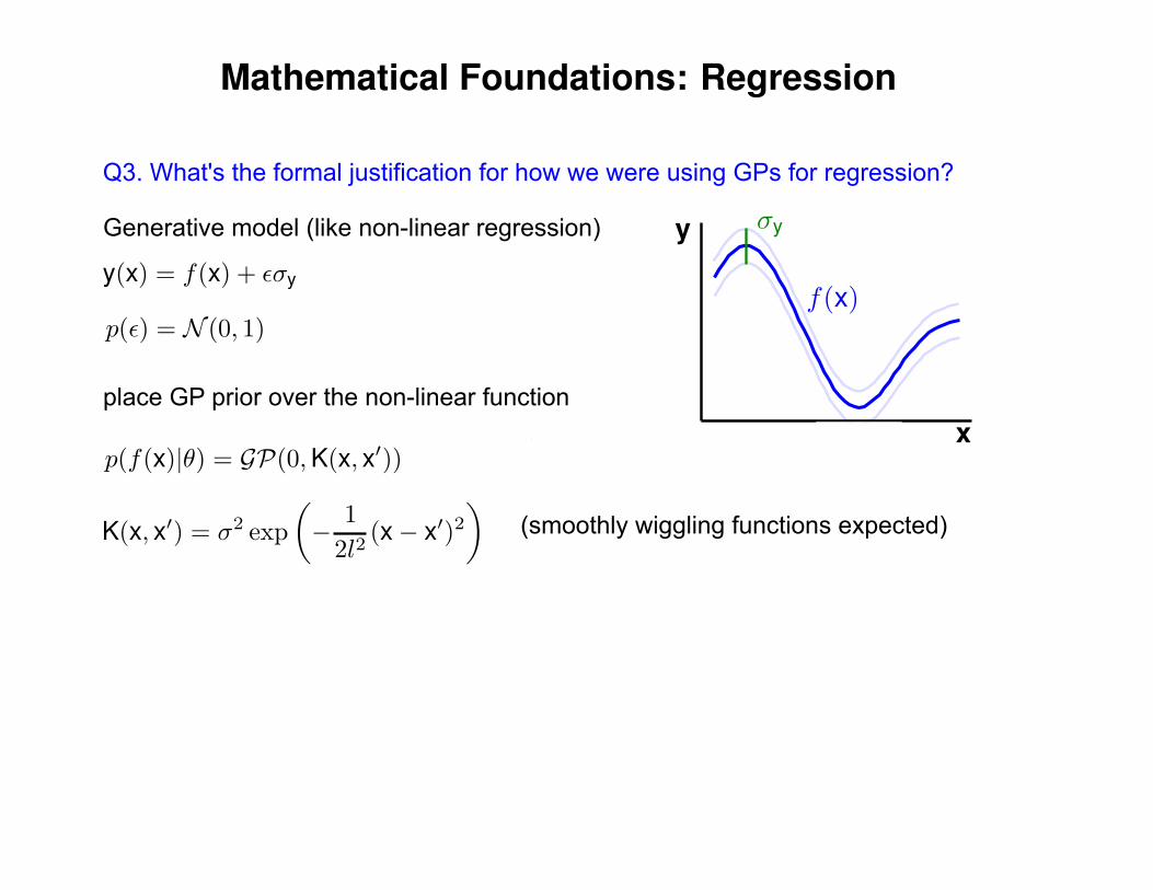
Q3. What's the formal justification for how we were using GPs for regression?
Mathematical Foundations: Regression
Q3. What's the formal justification for how we were using GPs for regression?
Generative model (like non-linear regression)
Mathematical Foundations: Regression
Q3. What's the formal justification for how we were using GPs for regression?
Generative model (like non-linear regression)
Mathematical Foundations: Regression
Q3. What's the formal justification for how we were using GPs for regression?
Generative model (like non-linear regression)
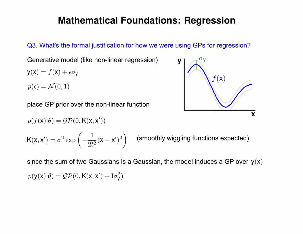
place GP prior over the non-linear function
(smoothly wiggling functions expected)
Mathematical Foundations: Regression
Q3. What's the formal justification for how we were using GPs for regression?
Generative model (like non-linear regression)
place GP prior over the non-linear function
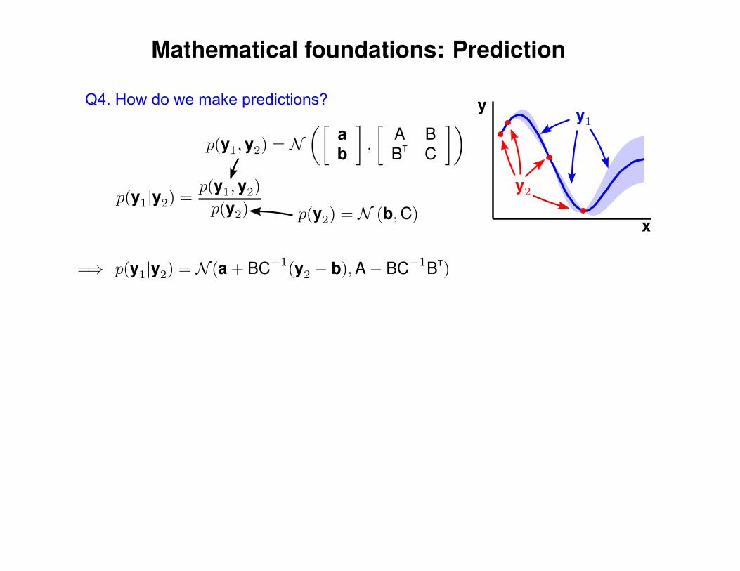
since the sum of two Gaussians is a Gaussian, the model induces a GP over
(smoothly wiggling functions expected)
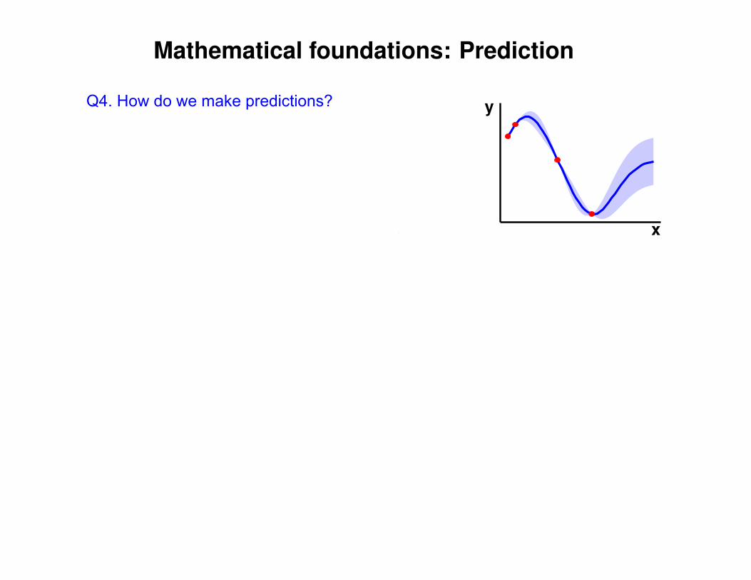
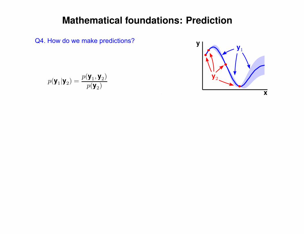
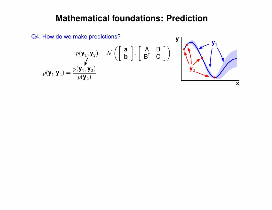
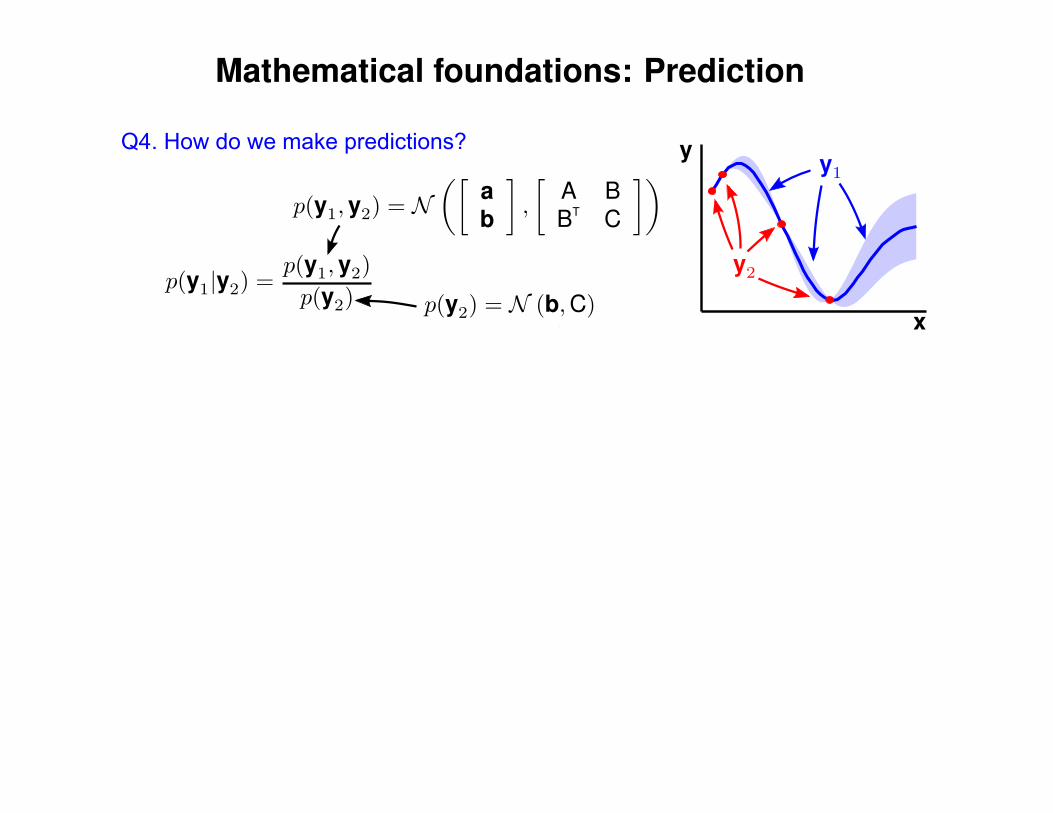
Mathematical foundations: Prediction
Q4. How do we make predictions?
Mathematical foundations: Prediction
Q4. How do we make predictions?
Mathematical foundations: Prediction
Q4. How do we make predictions?
Mathematical foundations: Prediction
Q4. How do we make predictions?
Mathematical foundations: Prediction
Q4. How do we make predictions?
Mathematical foundations: Prediction
Q4. How do we make predictions?
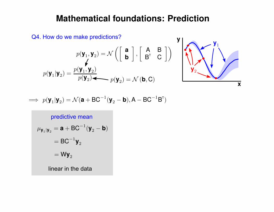
linear in the data
predictive mean
Mathematical foundations: Prediction
Q4. How do we make predictions?
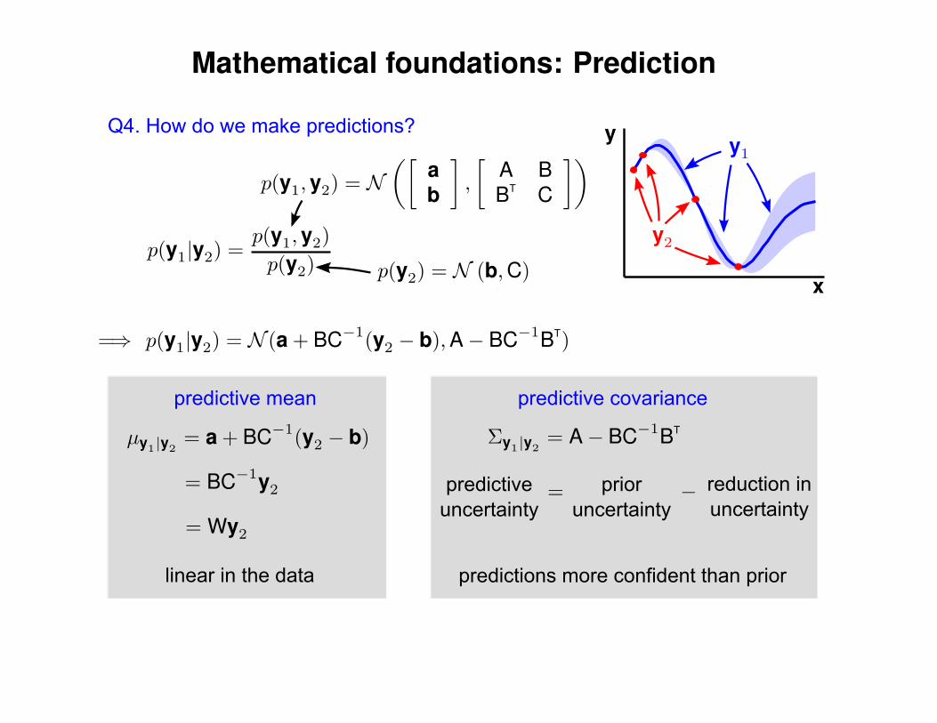
prior uncertainty
predictive uncertainty
reduction inuncertainty
linear in the data
predictive mean predictive covariance
predictions more confident than prior

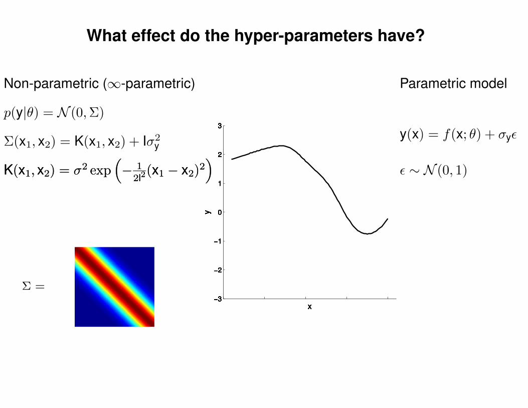
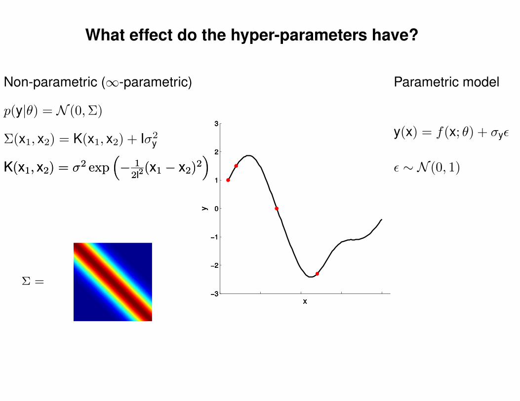
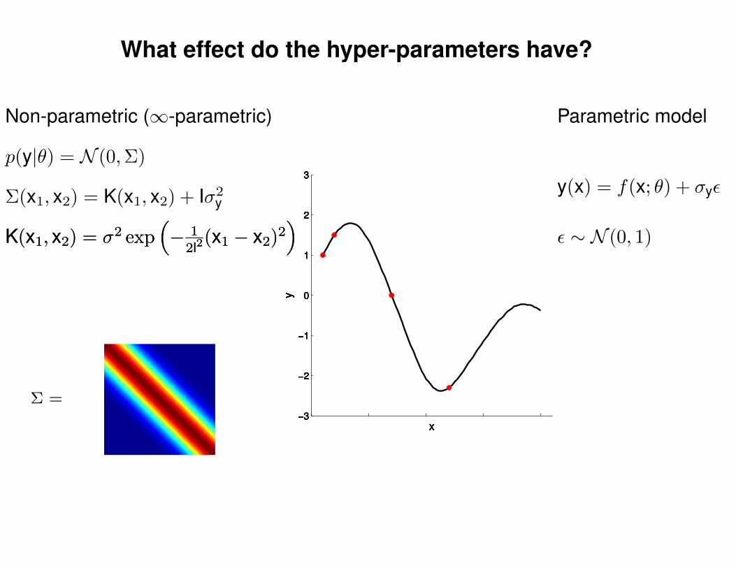
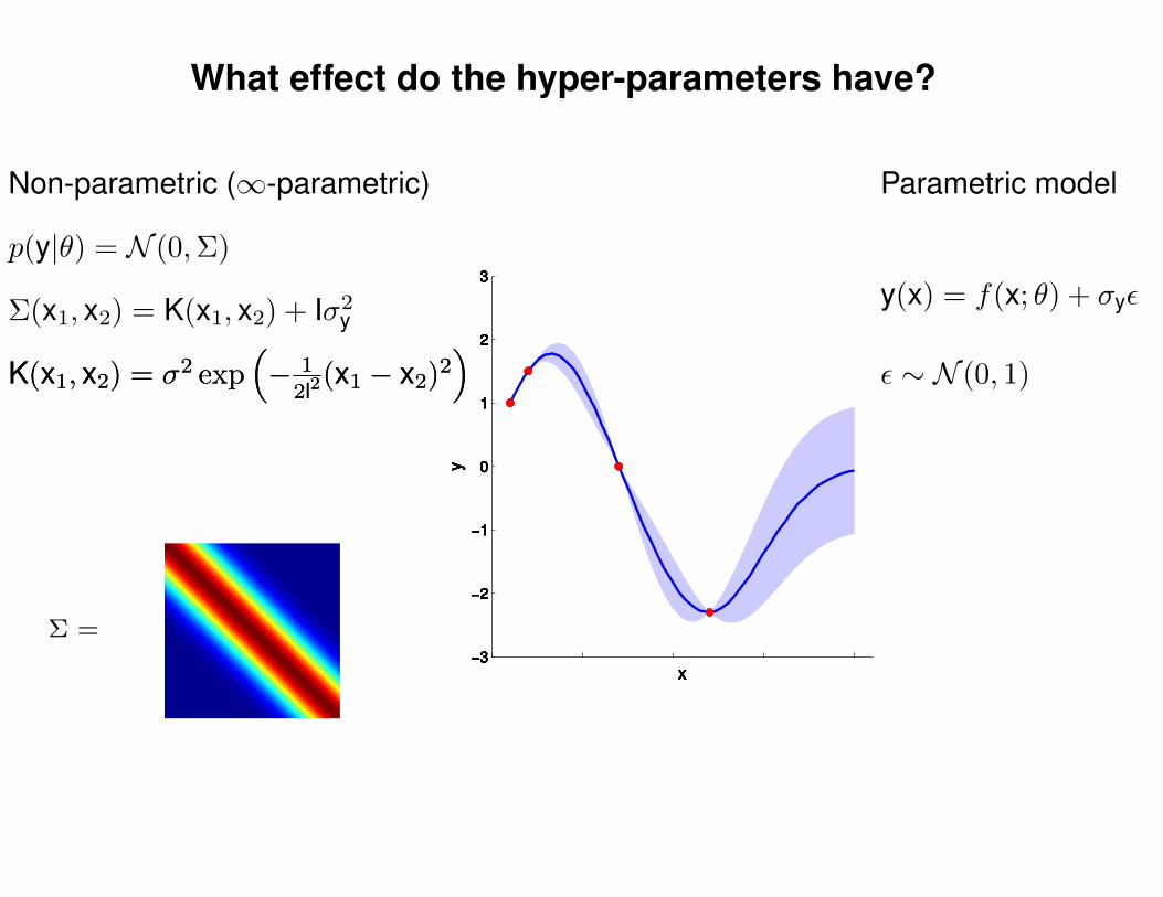
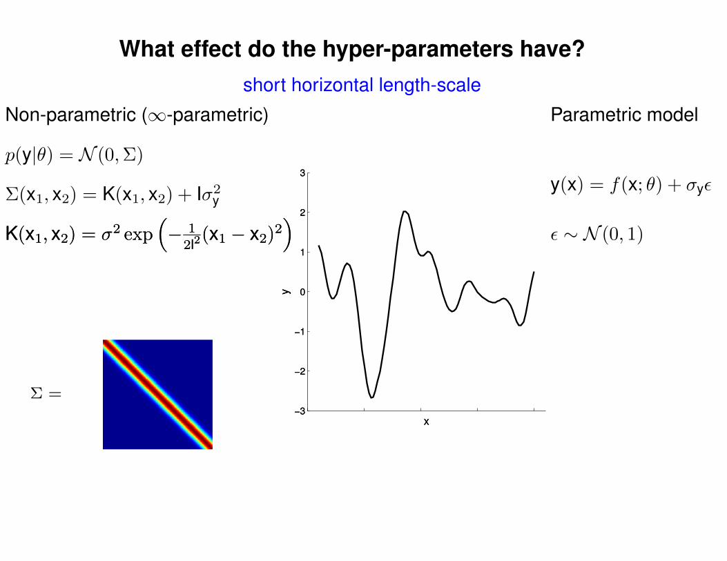
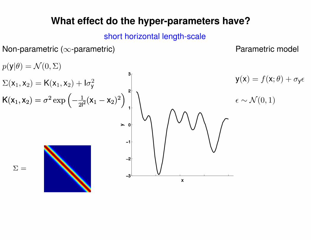
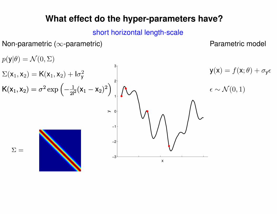
What effect do the hyper-parameters have?
−3
−2
−1
0
1
2
3
x
y
Σ =
Σ(x1, x2) = K(x1, x2) + Iσ2y
p(y|θ) = N (0,Σ)
Non-parametric (∞-parametric) Parametric model
y(x) = f(x; θ) + σyε
ε ∼ N (0, 1)K(x1, x2) = σ2 exp(− 1
2l2(x1 − x2)2
)K(x1, x2) = σ2 exp
(− 1
2l2(x1 − x2)2
)

What effect do the hyper-parameters have?
−3
−2
−1
0
1
2
3
x
y
−3
−2
−1
0
1
2
3
x
y
Σ =
Σ(x1, x2) = K(x1, x2) + Iσ2y
p(y|θ) = N (0,Σ)
Non-parametric (∞-parametric) Parametric model
y(x) = f(x; θ) + σyε
ε ∼ N (0, 1)K(x1, x2) = σ2 exp(− 1
2l2(x1 − x2)2
)K(x1, x2) = σ2 exp
(− 1
2l2(x1 − x2)2
)
What effect do the hyper-parameters have?
−3
−2
−1
0
1
2
3
x
y
−3
−2
−1
0
1
2
3
x
y
−3
−2
−1
0
1
2
3
x
y
Σ =
Σ(x1, x2) = K(x1, x2) + Iσ2y
p(y|θ) = N (0,Σ)
Non-parametric (∞-parametric) Parametric model
y(x) = f(x; θ) + σyε
ε ∼ N (0, 1)K(x1, x2) = σ2 exp(− 1
2l2(x1 − x2)2
)K(x1, x2) = σ2 exp
(− 1
2l2(x1 − x2)2
)

What effect do the hyper-parameters have?
−3
−2
−1
0
1
2
3
x
y
−3
−2
−1
0
1
2
3
x
y
−3
−2
−1
0
1
2
3
x
y
−3
−2
−1
0
1
2
3
x
y
−3
−2
−1
0
1
2
3
x
y
−3
−2
−1
0
1
2
3
x
y
Σ =
Σ(x1, x2) = K(x1, x2) + Iσ2y
p(y|θ) = N (0,Σ)
Non-parametric (∞-parametric) Parametric model
y(x) = f(x; θ) + σyε
ε ∼ N (0, 1)K(x1, x2) = σ2 exp(− 1
2l2(x1 − x2)2
)K(x1, x2) = σ2 exp
(− 1
2l2(x1 − x2)2
)
What effect do the hyper-parameters have?
−3
−2
−1
0
1
2
3
x
y
−3
−2
−1
0
1
2
3
x
y
−3
−2
−1
0
1
2
3
x
y
−3
−2
−1
0
1
2
3
x
y
−3
−2
−1
0
1
2
3
x
y
−3
−2
−1
0
1
2
3
x
y
−3
−2
−1
0
1
2
3
x
y
Σ =
Σ(x1, x2) = K(x1, x2) + Iσ2y
p(y|θ) = N (0,Σ)
Non-parametric (∞-parametric) Parametric model
y(x) = f(x; θ) + σyε
ε ∼ N (0, 1)K(x1, x2) = σ2 exp(− 1
2l2(x1 − x2)2
)K(x1, x2) = σ2 exp
(− 1
2l2(x1 − x2)2
)

What effect do the hyper-parameters have?
−3
−2
−1
0
1
2
3
x
y
−3
−2
−1
0
1
2
3
x
y
−3
−2
−1
0
1
2
3
x
y
−3
−2
−1
0
1
2
3
x
y
−3
−2
−1
0
1
2
3
x
y
−3
−2
−1
0
1
2
3
x
y
−3
−2
−1
0
1
2
3
x
y
−3
−2
−1
0
1
2
3
x
y
−3
−2
−1
0
1
2
3
x
y
−3
−2
−1
0
1
2
3
x
y
Σ =
Σ(x1, x2) = K(x1, x2) + Iσ2y
p(y|θ) = N (0,Σ)
Non-parametric (∞-parametric) Parametric model
y(x) = f(x; θ) + σyε
ε ∼ N (0, 1)K(x1, x2) = σ2 exp(− 1
2l2(x1 − x2)2
)K(x1, x2) = σ2 exp
(− 1
2l2(x1 − x2)2
)

What effect do the hyper-parameters have?
−3
−2
−1
0
1
2
3
x
y
Σ =
Σ(x1, x2) = K(x1, x2) + Iσ2y
p(y|θ) = N (0,Σ)
Non-parametric (∞-parametric) Parametric model
y(x) = f(x; θ) + σyε
ε ∼ N (0, 1)K(x1, x2) = σ2 exp(− 1
2l2(x1 − x2)2
)K(x1, x2) = σ2 exp
(− 1
2l2(x1 − x2)2
)

What effect do the hyper-parameters have?
−3
−2
−1
0
1
2
3
x
y
−3
−2
−1
0
1
2
3
x
y
Σ =
Σ(x1, x2) = K(x1, x2) + Iσ2y
p(y|θ) = N (0,Σ)
Non-parametric (∞-parametric) Parametric model
y(x) = f(x; θ) + σyε
ε ∼ N (0, 1)K(x1, x2) = σ2 exp(− 1
2l2(x1 − x2)2
)K(x1, x2) = σ2 exp
(− 1
2l2(x1 − x2)2
)
What effect do the hyper-parameters have?
−3
−2
−1
0
1
2
3
x
y
−3
−2
−1
0
1
2
3
x
y
−3
−2
−1
0
1
2
3
x
y
Σ =
Σ(x1, x2) = K(x1, x2) + Iσ2y
p(y|θ) = N (0,Σ)
Non-parametric (∞-parametric) Parametric model
y(x) = f(x; θ) + σyε
ε ∼ N (0, 1)K(x1, x2) = σ2 exp(− 1
2l2(x1 − x2)2
)K(x1, x2) = σ2 exp
(− 1
2l2(x1 − x2)2
)

What effect do the hyper-parameters have?
−3
−2
−1
0
1
2
3
x
y
−3
−2
−1
0
1
2
3
x
y
−3
−2
−1
0
1
2
3
x
y
−3
−2
−1
0
1
2
3
x
y
Σ =
Σ(x1, x2) = K(x1, x2) + Iσ2y
p(y|θ) = N (0,Σ)
Non-parametric (∞-parametric) Parametric model
y(x) = f(x; θ) + σyε
ε ∼ N (0, 1)K(x1, x2) = σ2 exp(− 1
2l2(x1 − x2)2
)K(x1, x2) = σ2 exp
(− 1
2l2(x1 − x2)2
)
What effect do the hyper-parameters have?
−3
−2
−1
0
1
2
3
x
y
−3
−2
−1
0
1
2
3
x
y
−3
−2
−1
0
1
2
3
x
y
−3
−2
−1
0
1
2
3
x
y
−3
−2
−1
0
1
2
3
x
y
Σ =
Σ(x1, x2) = K(x1, x2) + Iσ2y
p(y|θ) = N (0,Σ)
Non-parametric (∞-parametric) Parametric model
y(x) = f(x; θ) + σyε
ε ∼ N (0, 1)K(x1, x2) = σ2 exp(− 1
2l2(x1 − x2)2
)K(x1, x2) = σ2 exp
(− 1
2l2(x1 − x2)2
)

What effect do the hyper-parameters have?
−3
−2
−1
0
1
2
3
x
y
−3
−2
−1
0
1
2
3
x
y
−3
−2
−1
0
1
2
3
x
y
−3
−2
−1
0
1
2
3
x
y
−3
−2
−1
0
1
2
3
x
y
−3
−2
−1
0
1
2
3
x
y
−3
−2
−1
0
1
2
3
x
y
−3
−2
−1
0
1
2
3
x
y
−3
−2
−1
0
1
2
3
x
y
−3
−2
−1
0
1
2
3
x
y
Σ =
Σ(x1, x2) = K(x1, x2) + Iσ2y
p(y|θ) = N (0,Σ)
Non-parametric (∞-parametric) Parametric model
y(x) = f(x; θ) + σyε
ε ∼ N (0, 1)K(x1, x2) = σ2 exp(− 1
2l2(x1 − x2)2
)K(x1, x2) = σ2 exp
(− 1
2l2(x1 − x2)2
)

What effect do the hyper-parameters have?
−3
−2
−1
0
1
2
3
x
y
Σ =
short horizontal length-scale
Σ(x1, x2) = K(x1, x2) + Iσ2y
p(y|θ) = N (0,Σ)
Non-parametric (∞-parametric) Parametric model
y(x) = f(x; θ) + σyε
ε ∼ N (0, 1)K(x1, x2) = σ2 exp(− 1
2l2(x1 − x2)2
)K(x1, x2) = σ2 exp
(− 1
2l2(x1 − x2)2
)
What effect do the hyper-parameters have?
−3
−2
−1
0
1
2
3
x
y
−3
−2
−1
0
1
2
3
x
y
Σ =
short horizontal length-scale
Σ(x1, x2) = K(x1, x2) + Iσ2y
p(y|θ) = N (0,Σ)
Non-parametric (∞-parametric) Parametric model
y(x) = f(x; θ) + σyε
ε ∼ N (0, 1)K(x1, x2) = σ2 exp(− 1
2l2(x1 − x2)2
)K(x1, x2) = σ2 exp
(− 1
2l2(x1 − x2)2
)

What effect do the hyper-parameters have?
−3
−2
−1
0
1
2
3
x
y
−3
−2
−1
0
1
2
3
x
y
−3
−2
−1
0
1
2
3
x
y
−3
−2
−1
0
1
2
3
x
y
Σ =
short horizontal length-scale
Σ(x1, x2) = K(x1, x2) + Iσ2y
p(y|θ) = N (0,Σ)
Non-parametric (∞-parametric) Parametric model
y(x) = f(x; θ) + σyε
ε ∼ N (0, 1)K(x1, x2) = σ2 exp(− 1
2l2(x1 − x2)2
)K(x1, x2) = σ2 exp
(− 1
2l2(x1 − x2)2
)
What effect do the hyper-parameters have?
−3
−2
−1
0
1
2
3
x
y
−3
−2
−1
0
1
2
3
x
y
−3
−2
−1
0
1
2
3
x
y
−3
−2
−1
0
1
2
3
x
y
−3
−2
−1
0
1
2
3
x
y
Σ =
short horizontal length-scale
Σ(x1, x2) = K(x1, x2) + Iσ2y
p(y|θ) = N (0,Σ)
Non-parametric (∞-parametric) Parametric model
y(x) = f(x; θ) + σyε
ε ∼ N (0, 1)K(x1, x2) = σ2 exp(− 1
2l2(x1 − x2)2
)K(x1, x2) = σ2 exp
(− 1
2l2(x1 − x2)2
)

What effect do the hyper-parameters have?
−3
−2
−1
0
1
2
3
x
y
−3
−2
−1
0
1
2
3
x
y
−3
−2
−1
0
1
2
3
x
y
−3
−2
−1
0
1
2
3
x
y
−3
−2
−1
0
1
2
3
x
y
−3
−2
−1
0
1
2
3
x
y
−3
−2
−1
0
1
2
3
x
y
Σ =
Σ(x1, x2) = K(x1, x2) + Iσ2y
short horizontal length-scale
p(y|θ) = N (0,Σ)
Non-parametric (∞-parametric) Parametric model
y(x) = f(x; θ) + σyε
ε ∼ N (0, 1)K(x1, x2) = σ2 exp(− 1
2l2(x1 − x2)2
)K(x1, x2) = σ2 exp
(− 1
2l2(x1 − x2)2
)

What effect do the hyper-parameters have?
−3
−2
−1
0
1
2
3
x
y
−3
−2
−1
0
1
2
3
x
y
−3
−2
−1
0
1
2
3
x
y
−3
−2
−1
0
1
2
3
x
y
−3
−2
−1
0
1
2
3
x
y
−3
−2
−1
0
1
2
3
x
y
−3
−2
−1
0
1
2
3
x
y
−3
−2
−1
0
1
2
3
x
y
−3
−2
−1
0
1
2
3
x
y
−3
−2
−1
0
1
2
3
x
y
Σ =
Σ(x1, x2) = K(x1, x2) + Iσ2y
short horizontal length-scale
p(y|θ) = N (0,Σ)
Non-parametric (∞-parametric) Parametric model
y(x) = f(x; θ) + σyε
ε ∼ N (0, 1)K(x1, x2) = σ2 exp(− 1
2l2(x1 − x2)2
)K(x1, x2) = σ2 exp
(− 1
2l2(x1 − x2)2
)
What effect do the hyper-parameters have?
−3
−2
−1
0
1
2
3
x
y
Σ =
Σ(x1, x2) = K(x1, x2) + Iσ2y
p(y|θ) = N (0,Σ)
Non-parametric (∞-parametric)
short horizontal length-scale
Parametric model
y(x) = f(x; θ) + σyε
ε ∼ N (0, 1)K(x1, x2) = σ2 exp(− 1
2l2(x1 − x2)2
)K(x1, x2) = σ2 exp
(− 1
2l2(x1 − x2)2
)

What effect do the hyper-parameters have?
−3
−2
−1
0
1
2
3
x
y
−3
−2
−1
0
1
2
3
x
y
Σ =
Σ(x1, x2) = K(x1, x2) + Iσ2y
short horizontal length-scale
p(y|θ) = N (0,Σ)
Non-parametric (∞-parametric) Parametric model
y(x) = f(x; θ) + σyε
ε ∼ N (0, 1)K(x1, x2) = σ2 exp(− 1
2l2(x1 − x2)2
)K(x1, x2) = σ2 exp
(− 1
2l2(x1 − x2)2
)

What effect do the hyper-parameters have?
−3
−2
−1
0
1
2
3
x
y
−3
−2
−1
0
1
2
3
x
y
−3
−2
−1
0
1
2
3
x
y
Σ =
Σ(x1, x2) = K(x1, x2) + Iσ2y
p(y|θ) = N (0,Σ)
Non-parametric (∞-parametric)
short horizontal length-scale
Parametric model
y(x) = f(x; θ) + σyε
ε ∼ N (0, 1)K(x1, x2) = σ2 exp(− 1
2l2(x1 − x2)2
)K(x1, x2) = σ2 exp
(− 1
2l2(x1 − x2)2
)

What effect do the hyper-parameters have?
−3
−2
−1
0
1
2
3
x
y
−3
−2
−1
0
1
2
3
x
y
−3
−2
−1
0
1
2
3
x
y
−3
−2
−1
0
1
2
3
x
y
Σ =
Σ(x1, x2) = K(x1, x2) + Iσ2y
short horizontal length-scale
p(y|θ) = N (0,Σ)
Non-parametric (∞-parametric) Parametric model
y(x) = f(x; θ) + σyε
ε ∼ N (0, 1)K(x1, x2) = σ2 exp(− 1
2l2(x1 − x2)2
)K(x1, x2) = σ2 exp
(− 1
2l2(x1 − x2)2
)

What effect do the hyper-parameters have?
−3
−2
−1
0
1
2
3
x
y
−3
−2
−1
0
1
2
3
x
y
−3
−2
−1
0
1
2
3
x
y
−3
−2
−1
0
1
2
3
x
y
−3
−2
−1
0
1
2
3
x
y
−3
−2
−1
0
1
2
3
x
y
Σ =
Σ(x1, x2) = K(x1, x2) + Iσ2y
short horizontal length-scale
p(y|θ) = N (0,Σ)
Non-parametric (∞-parametric) Parametric model
y(x) = f(x; θ) + σyε
ε ∼ N (0, 1)K(x1, x2) = σ2 exp(− 1
2l2(x1 − x2)2
)K(x1, x2) = σ2 exp
(− 1
2l2(x1 − x2)2
)
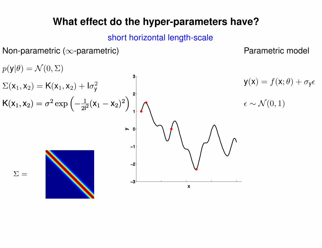
What effect do the hyper-parameters have?
−3
−2
−1
0
1
2
3
x
y
−3
−2
−1
0
1
2
3
x
y
−3
−2
−1
0
1
2
3
x
y
−3
−2
−1
0
1
2
3
x
y
−3
−2
−1
0
1
2
3
x
y
−3
−2
−1
0
1
2
3
x
y
−3
−2
−1
0
1
2
3
x
y
Σ =
Σ(x1, x2) = K(x1, x2) + Iσ2y
p(y|θ) = N (0,Σ)
Non-parametric (∞-parametric)
short horizontal length-scale
Parametric model
y(x) = f(x; θ) + σyε
ε ∼ N (0, 1)K(x1, x2) = σ2 exp(− 1
2l2(x1 − x2)2
)K(x1, x2) = σ2 exp
(− 1
2l2(x1 − x2)2
)

What effect do the hyper-parameters have?
−3
−2
−1
0
1
2
3
x
y
−3
−2
−1
0
1
2
3
x
y
−3
−2
−1
0
1
2
3
x
y
−3
−2
−1
0
1
2
3
x
y
−3
−2
−1
0
1
2
3
x
y
−3
−2
−1
0
1
2
3
x
y
−3
−2
−1
0
1
2
3
x
y
−3
−2
−1
0
1
2
3
x
y
Σ =
Σ(x1, x2) = K(x1, x2) + Iσ2y
p(y|θ) = N (0,Σ)
Non-parametric (∞-parametric)
short horizontal length-scale
Parametric model
y(x) = f(x; θ) + σyε
ε ∼ N (0, 1)K(x1, x2) = σ2 exp(− 1
2l2(x1 − x2)2
)K(x1, x2) = σ2 exp
(− 1
2l2(x1 − x2)2
)
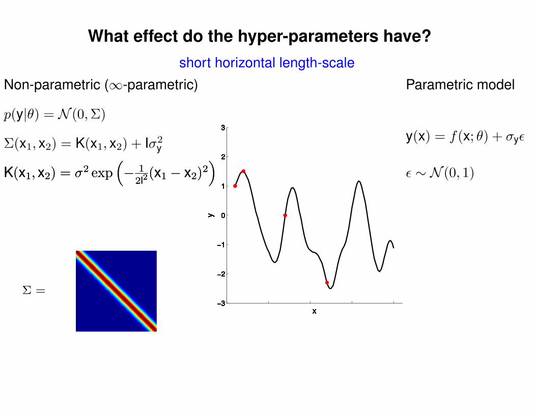
What effect do the hyper-parameters have?
−3
−2
−1
0
1
2
3
x
y
−3
−2
−1
0
1
2
3
x
y
−3
−2
−1
0
1
2
3
x
y
−3
−2
−1
0
1
2
3
x
y
−3
−2
−1
0
1
2
3
x
y
−3
−2
−1
0
1
2
3
x
y
−3
−2
−1
0
1
2
3
x
y
−3
−2
−1
0
1
2
3
x
y
−3
−2
−1
0
1
2
3
x
y
−3
−2
−1
0
1
2
3
x
y
Σ =
Σ(x1, x2) = K(x1, x2) + Iσ2y
p(y|θ) = N (0,Σ)
Non-parametric (∞-parametric)
short horizontal length-scale
Parametric model
y(x) = f(x; θ) + σyε
ε ∼ N (0, 1)K(x1, x2) = σ2 exp(− 1
2l2(x1 − x2)2
)K(x1, x2) = σ2 exp
(− 1
2l2(x1 − x2)2
)
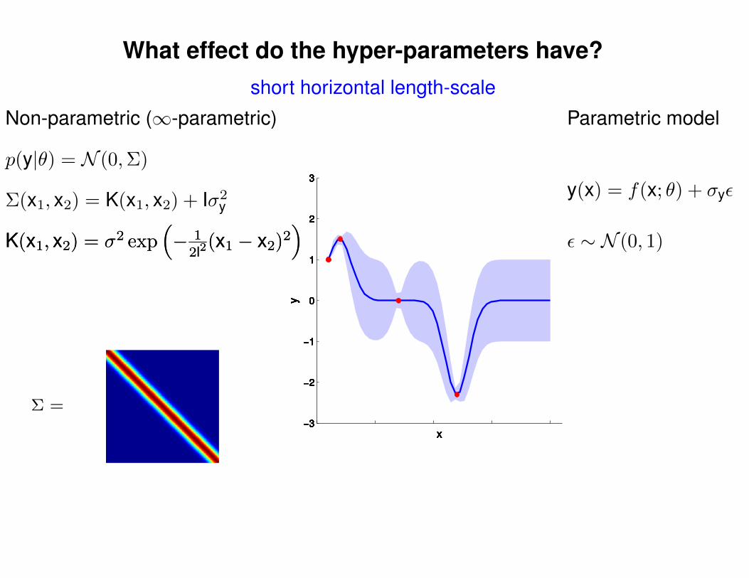
What effect do the hyper-parameters have?
−3
−2
−1
0
1
2
3
x
y
−3
−2
−1
0
1
2
3
x
y
−3
−2
−1
0
1
2
3
x
y
−3
−2
−1
0
1
2
3
x
y
−3
−2
−1
0
1
2
3
x
y
−3
−2
−1
0
1
2
3
x
y
−3
−2
−1
0
1
2
3
x
y
−3
−2
−1
0
1
2
3
x
y
−3
−2
−1
0
1
2
3
x
y
−3
−2
−1
0
1
2
3
x
y
Σ =
Σ(x1, x2) = K(x1, x2) + Iσ2y
p(y|θ) = N (0,Σ)
Non-parametric (∞-parametric)
short horizontal length-scale
Parametric model
y(x) = f(x; θ) + σyε
ε ∼ N (0, 1)K(x1, x2) = σ2 exp(− 1
2l2(x1 − x2)2
)K(x1, x2) = σ2 exp
(− 1
2l2(x1 − x2)2
)
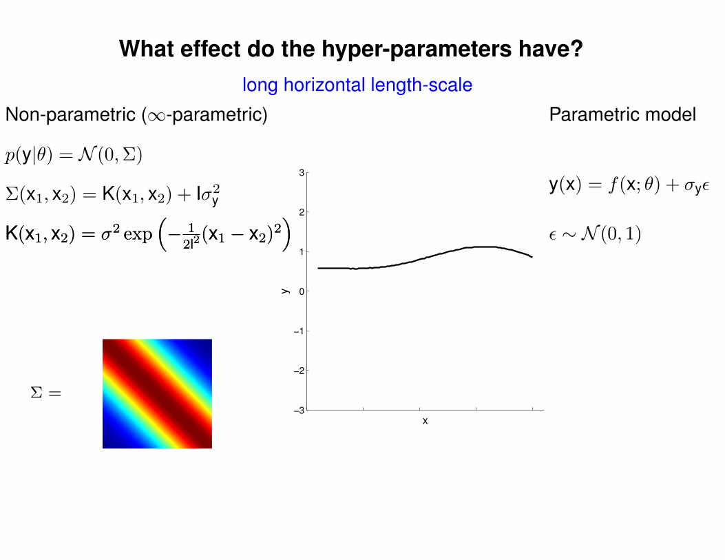
What effect do the hyper-parameters have?
−3
−2
−1
0
1
2
3
x
y
Σ =
long horizontal length-scale
Σ(x1, x2) = K(x1, x2) + Iσ2y
p(y|θ) = N (0,Σ)
Non-parametric (∞-parametric) Parametric model
y(x) = f(x; θ) + σyε
ε ∼ N (0, 1)K(x1, x2) = σ2 exp(− 1
2l2(x1 − x2)2
)K(x1, x2) = σ2 exp
(− 1
2l2(x1 − x2)2
)

What effect do the hyper-parameters have?
−3
−2
−1
0
1
2
3
x
y
−3
−2
−1
0
1
2
3
x
y
−3
−2
−1
0
1
2
3
x
y
Σ =
Σ(x1, x2) = K(x1, x2) + Iσ2y
long horizontal length-scale
p(y|θ) = N (0,Σ)
Non-parametric (∞-parametric) Parametric model
y(x) = f(x; θ) + σyε
ε ∼ N (0, 1)K(x1, x2) = σ2 exp(− 1
2l2(x1 − x2)2
)K(x1, x2) = σ2 exp
(− 1
2l2(x1 − x2)2
)

What effect do the hyper-parameters have?
−3
−2
−1
0
1
2
3
x
y
−3
−2
−1
0
1
2
3
x
y
−3
−2
−1
0
1
2
3
x
y
−3
−2
−1
0
1
2
3
x
y
−3
−2
−1
0
1
2
3
x
y
Σ =
Σ(x1, x2) = K(x1, x2) + Iσ2y
long horizontal length-scale
p(y|θ) = N (0,Σ)
Non-parametric (∞-parametric) Parametric model
y(x) = f(x; θ) + σyε
ε ∼ N (0, 1)K(x1, x2) = σ2 exp(− 1
2l2(x1 − x2)2
)K(x1, x2) = σ2 exp
(− 1
2l2(x1 − x2)2
)
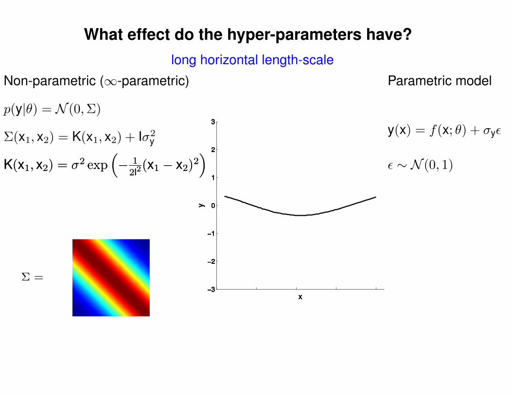
What effect do the hyper-parameters have?
−3
−2
−1
0
1
2
3
x
y
−3
−2
−1
0
1
2
3
x
y
−3
−2
−1
0
1
2
3
x
y
−3
−2
−1
0
1
2
3
x
y
−3
−2
−1
0
1
2
3
x
y
−3
−2
−1
0
1
2
3
x
y
−3
−2
−1
0
1
2
3
x
y
−3
−2
−1
0
1
2
3
x
y
Σ =
Σ(x1, x2) = K(x1, x2) + Iσ2y
long horizontal length-scale
p(y|θ) = N (0,Σ)
Non-parametric (∞-parametric) Parametric model
y(x) = f(x; θ) + σyε
ε ∼ N (0, 1)K(x1, x2) = σ2 exp(− 1
2l2(x1 − x2)2
)K(x1, x2) = σ2 exp
(− 1
2l2(x1 − x2)2
)
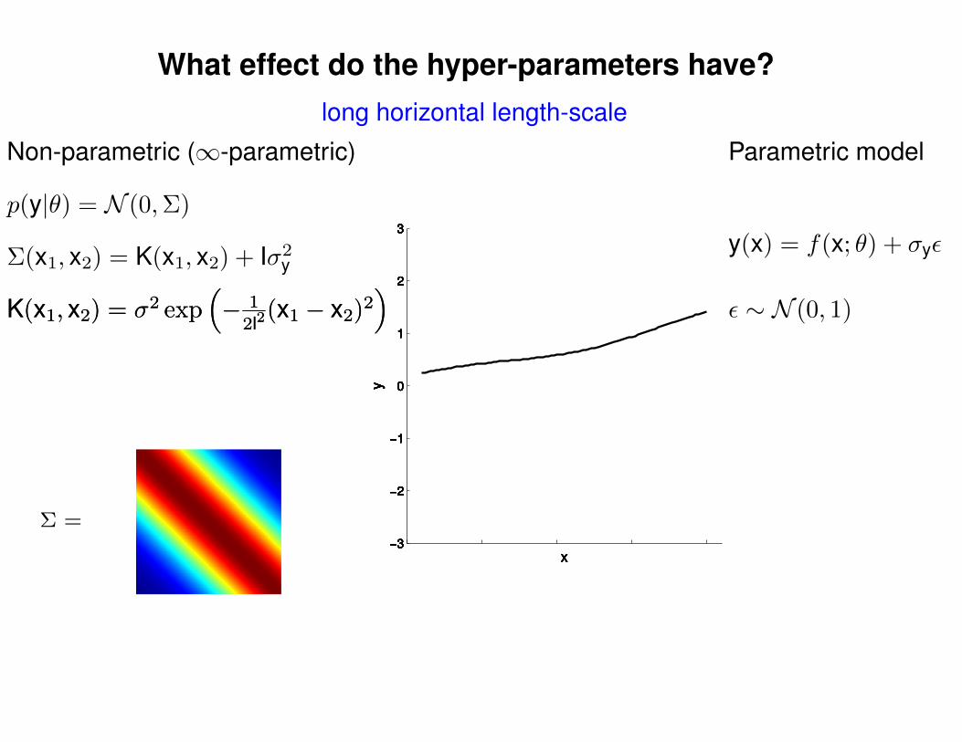
What effect do the hyper-parameters have?
−3
−2
−1
0
1
2
3
x
y
−3
−2
−1
0
1
2
3
x
y
−3
−2
−1
0
1
2
3
x
y
−3
−2
−1
0
1
2
3
x
y
−3
−2
−1
0
1
2
3
x
y
−3
−2
−1
0
1
2
3
x
y
−3
−2
−1
0
1
2
3
x
y
−3
−2
−1
0
1
2
3
x
y
−3
−2
−1
0
1
2
3
x
y
−3
−2
−1
0
1
2
3
x
y
Σ =
Σ(x1, x2) = K(x1, x2) + Iσ2y
long horizontal length-scale
p(y|θ) = N (0,Σ)
Non-parametric (∞-parametric) Parametric model
y(x) = f(x; θ) + σyε
ε ∼ N (0, 1)K(x1, x2) = σ2 exp(− 1
2l2(x1 − x2)2
)K(x1, x2) = σ2 exp
(− 1
2l2(x1 − x2)2
)

What effect do the hyper-parameters have?
−3
−2
−1
0
1
2
3
x
y
−3
−2
−1
0
1
2
3
x
y
−3
−2
−1
0
1
2
3
x
y
−3
−2
−1
0
1
2
3
x
y
−3
−2
−1
0
1
2
3
x
y
−3
−2
−1
0
1
2
3
x
y
−3
−2
−1
0
1
2
3
x
y
−3
−2
−1
0
1
2
3
x
y
Σ =
Σ(x1, x2) = K(x1, x2) + Iσ2y
long horizontal length-scale
p(y|θ) = N (0,Σ)
Non-parametric (∞-parametric) Parametric model
y(x) = f(x; θ) + σyε
ε ∼ N (0, 1)K(x1, x2) = σ2 exp(− 1
2l2(x1 − x2)2
)K(x1, x2) = σ2 exp
(− 1
2l2(x1 − x2)2
)
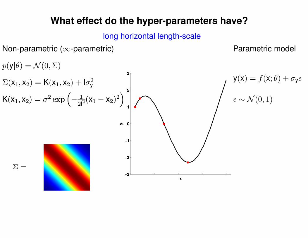
What effect do the hyper-parameters have?
−3
−2
−1
0
1
2
3
x
y
−3
−2
−1
0
1
2
3
x
y
−3
−2
−1
0
1
2
3
x
y
−3
−2
−1
0
1
2
3
x
y
−3
−2
−1
0
1
2
3
x
y
−3
−2
−1
0
1
2
3
x
y
−3
−2
−1
0
1
2
3
x
y
−3
−2
−1
0
1
2
3
x
y
−3
−2
−1
0
1
2
3
x
y
−3
−2
−1
0
1
2
3
x
y
Σ =
Σ(x1, x2) = K(x1, x2) + Iσ2y
long horizontal length-scale
p(y|θ) = N (0,Σ)
Non-parametric (∞-parametric) Parametric model
y(x) = f(x; θ) + σyε
ε ∼ N (0, 1)K(x1, x2) = σ2 exp(− 1
2l2(x1 − x2)2
)K(x1, x2) = σ2 exp
(− 1
2l2(x1 − x2)2
)
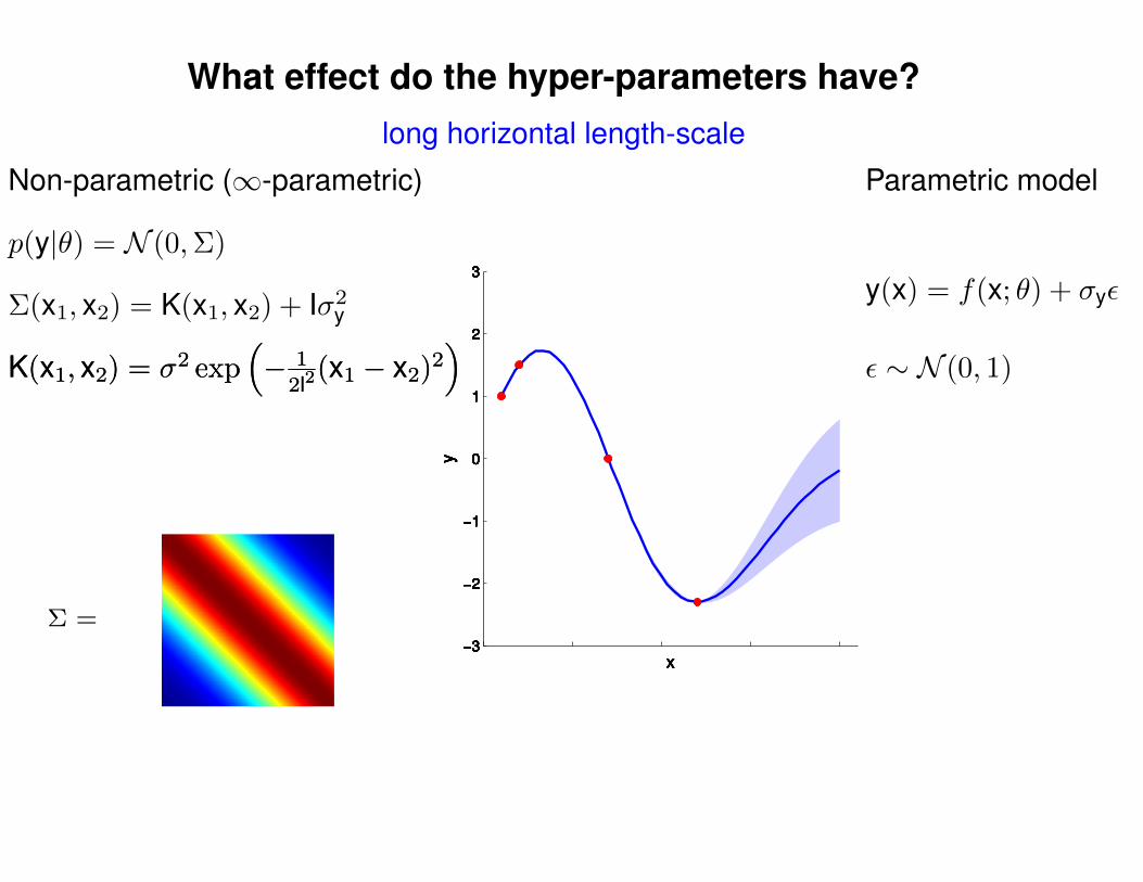
What effect do the hyper-parameters have?
−3
−2
−1
0
1
2
3
x
y
−3
−2
−1
0
1
2
3
x
y
−3
−2
−1
0
1
2
3
x
y
−3
−2
−1
0
1
2
3
x
y
−3
−2
−1
0
1
2
3
x
y
−3
−2
−1
0
1
2
3
x
y
−3
−2
−1
0
1
2
3
x
y
−3
−2
−1
0
1
2
3
x
y
−3
−2
−1
0
1
2
3
x
y
−3
−2
−1
0
1
2
3
x
y
Σ =
Σ(x1, x2) = K(x1, x2) + Iσ2y
long horizontal length-scale
p(y|θ) = N (0,Σ)
Non-parametric (∞-parametric) Parametric model
y(x) = f(x; θ) + σyε
ε ∼ N (0, 1)K(x1, x2) = σ2 exp(− 1
2l2(x1 − x2)2
)K(x1, x2) = σ2 exp
(− 1
2l2(x1 − x2)2
)

What effect do the hyper-parameters have?
−3
−2
−1
0
1
2
3
x
y
Σ =
Σ(x1, x2) = K(x1, x2) + Iσ2y
small vertical scale
p(y|θ) = N (0,Σ)
Non-parametric (∞-parametric) Parametric model
y(x) = f(x; θ) + σyε
ε ∼ N (0, 1)K(x1, x2) = σ2 exp(− 1
2l2(x1 − x2)2
)K(x1, x2) = σ2 exp
(− 1
2l2(x1 − x2)2
)

What effect do the hyper-parameters have?
−3
−2
−1
0
1
2
3
x
y
−3
−2
−1
0
1
2
3
x
y
−3
−2
−1
0
1
2
3
x
y
Σ =
Σ(x1, x2) = K(x1, x2) + Iσ2y
small vertical scale
p(y|θ) = N (0,Σ)
Non-parametric (∞-parametric) Parametric model
y(x) = f(x; θ) + σyε
ε ∼ N (0, 1)K(x1, x2) = σ2 exp(− 1
2l2(x1 − x2)2
)K(x1, x2) = σ2 exp
(− 1
2l2(x1 − x2)2
)
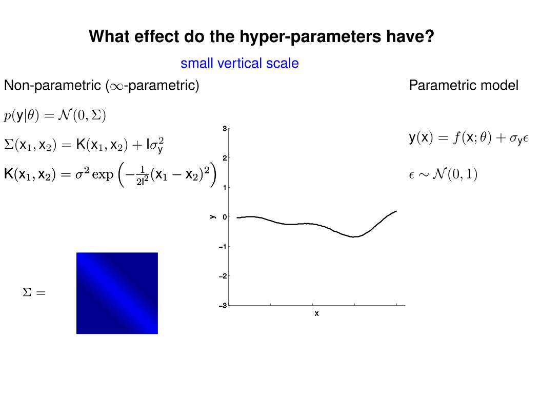
What effect do the hyper-parameters have?
−3
−2
−1
0
1
2
3
x
y
−3
−2
−1
0
1
2
3
x
y
−3
−2
−1
0
1
2
3
x
y
−3
−2
−1
0
1
2
3
x
y
−3
−2
−1
0
1
2
3
x
y
−3
−2
−1
0
1
2
3
x
y
−3
−2
−1
0
1
2
3
x
y
Σ =
Σ(x1, x2) = K(x1, x2) + Iσ2y
small vertical scale
p(y|θ) = N (0,Σ)
Non-parametric (∞-parametric) Parametric model
y(x) = f(x; θ) + σyε
ε ∼ N (0, 1)K(x1, x2) = σ2 exp(− 1
2l2(x1 − x2)2
)K(x1, x2) = σ2 exp
(− 1
2l2(x1 − x2)2
)
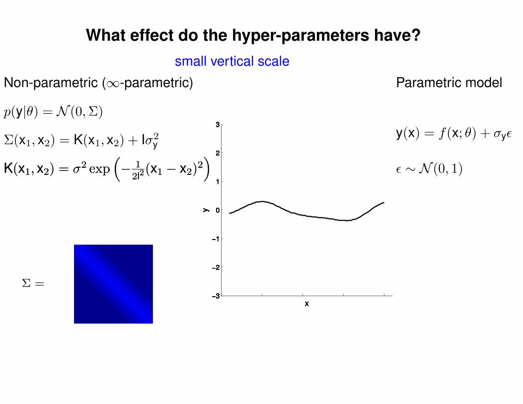
What effect do the hyper-parameters have?
−3
−2
−1
0
1
2
3
x
y
−3
−2
−1
0
1
2
3
x
y
−3
−2
−1
0
1
2
3
x
y
−3
−2
−1
0
1
2
3
x
y
−3
−2
−1
0
1
2
3
x
y
−3
−2
−1
0
1
2
3
x
y
−3
−2
−1
0
1
2
3
x
y
−3
−2
−1
0
1
2
3
x
y
Σ =
Σ(x1, x2) = K(x1, x2) + Iσ2y
small vertical scale
p(y|θ) = N (0,Σ)
Non-parametric (∞-parametric) Parametric model
y(x) = f(x; θ) + σyε
ε ∼ N (0, 1)K(x1, x2) = σ2 exp(− 1
2l2(x1 − x2)2
)K(x1, x2) = σ2 exp
(− 1
2l2(x1 − x2)2
)
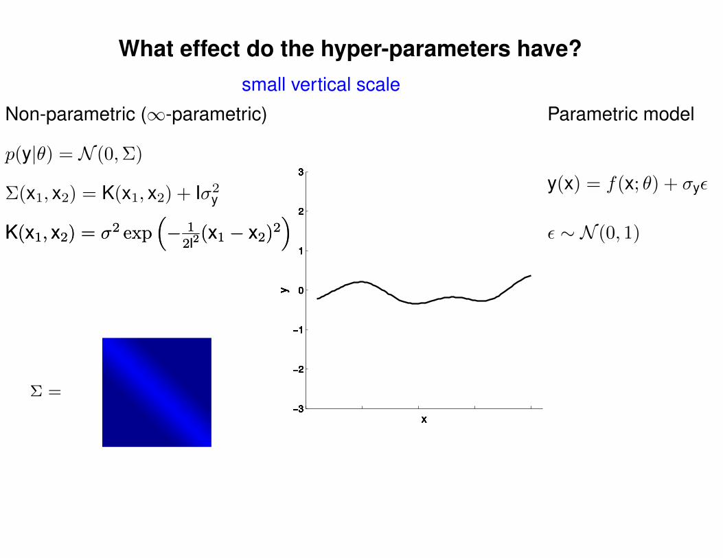
What effect do the hyper-parameters have?
−3
−2
−1
0
1
2
3
x
y
−3
−2
−1
0
1
2
3
x
y
−3
−2
−1
0
1
2
3
x
y
−3
−2
−1
0
1
2
3
x
y
−3
−2
−1
0
1
2
3
x
y
−3
−2
−1
0
1
2
3
x
y
−3
−2
−1
0
1
2
3
x
y
−3
−2
−1
0
1
2
3
x
y
−3
−2
−1
0
1
2
3
x
y
−3
−2
−1
0
1
2
3
x
y
Σ =
Σ(x1, x2) = K(x1, x2) + Iσ2y
small vertical scale
p(y|θ) = N (0,Σ)
Non-parametric (∞-parametric) Parametric model
y(x) = f(x; θ) + σyε
ε ∼ N (0, 1)K(x1, x2) = σ2 exp(− 1
2l2(x1 − x2)2
)K(x1, x2) = σ2 exp
(− 1
2l2(x1 − x2)2
)

What effect do the hyper-parameters have?
−3
−2
−1
0
1
2
3
x
y
Σ =
Σ(x1, x2) = K(x1, x2) + Iσ2y
small vertical scale
p(y|θ) = N (0,Σ)
Non-parametric (∞-parametric) Parametric model
y(x) = f(x; θ) + σyε
ε ∼ N (0, 1)K(x1, x2) = σ2 exp(− 1
2l2(x1 − x2)2
)K(x1, x2) = σ2 exp
(− 1
2l2(x1 − x2)2
)

What effect do the hyper-parameters have?
−3
−2
−1
0
1
2
3
x
y
−3
−2
−1
0
1
2
3
x
y
Σ =
Σ(x1, x2) = K(x1, x2) + Iσ2y
small vertical scale
p(y|θ) = N (0,Σ)
Non-parametric (∞-parametric) Parametric model
y(x) = f(x; θ) + σyε
ε ∼ N (0, 1)K(x1, x2) = σ2 exp(− 1
2l2(x1 − x2)2
)K(x1, x2) = σ2 exp
(− 1
2l2(x1 − x2)2
)
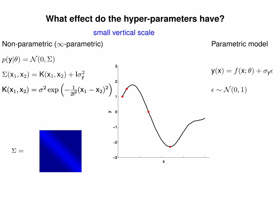
What effect do the hyper-parameters have?
−3
−2
−1
0
1
2
3
x
y
−3
−2
−1
0
1
2
3
x
y
−3
−2
−1
0
1
2
3
x
y
−3
−2
−1
0
1
2
3
x
y
−3
−2
−1
0
1
2
3
x
y
−3
−2
−1
0
1
2
3
x
y
−3
−2
−1
0
1
2
3
x
y
−3
−2
−1
0
1
2
3
x
y
−3
−2
−1
0
1
2
3
x
y
−3
−2
−1
0
1
2
3
x
y
Σ =
Σ(x1, x2) = K(x1, x2) + Iσ2y
small vertical scale
p(y|θ) = N (0,Σ)
Non-parametric (∞-parametric) Parametric model
y(x) = f(x; θ) + σyε
ε ∼ N (0, 1)K(x1, x2) = σ2 exp(− 1
2l2(x1 − x2)2
)K(x1, x2) = σ2 exp
(− 1
2l2(x1 − x2)2
)
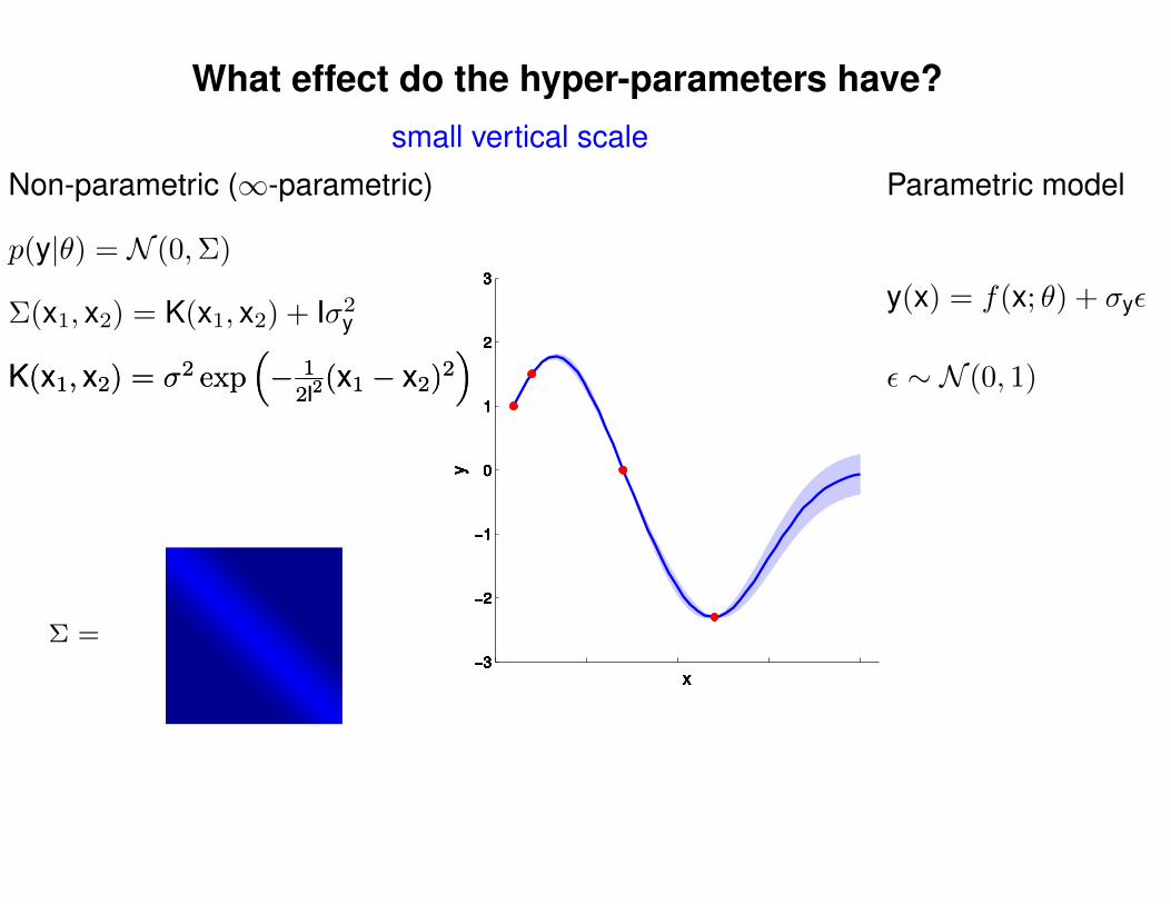
What effect do the hyper-parameters have?
−3
−2
−1
0
1
2
3
x
y
−3
−2
−1
0
1
2
3
x
y
−3
−2
−1
0
1
2
3
x
y
−3
−2
−1
0
1
2
3
x
y
−3
−2
−1
0
1
2
3
x
y
−3
−2
−1
0
1
2
3
x
y
−3
−2
−1
0
1
2
3
x
y
−3
−2
−1
0
1
2
3
x
y
−3
−2
−1
0
1
2
3
x
y
−3
−2
−1
0
1
2
3
x
y
Σ =
Σ(x1, x2) = K(x1, x2) + Iσ2y
small vertical scale
p(y|θ) = N (0,Σ)
Non-parametric (∞-parametric) Parametric model
y(x) = f(x; θ) + σyε
ε ∼ N (0, 1)K(x1, x2) = σ2 exp(− 1
2l2(x1 − x2)2
)K(x1, x2) = σ2 exp
(− 1
2l2(x1 − x2)2
)
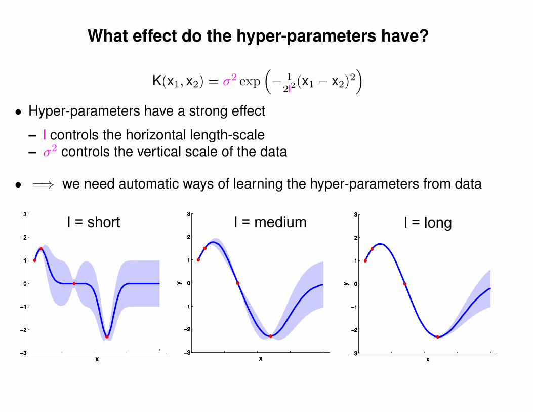
What effect do the hyper-parameters have?
K(x1, x2) = σ2 exp(− 1
2l2(x1 − x2)2
)• Hyper-parameters have a strong effect
– l controls the horizontal length-scale– σ2 controls the vertical scale of the data
• =⇒ we need automatic ways of learning the hyper-parameters from data
−3
−2
−1
0
1
2
3
x
y
−3
−2
−1
0
1
2
3
x
y
−3
−2
−1
0
1
2
3
x
y
−3
−2
−1
0
1
2
3
x
y
−3
−2
−1
0
1
2
3
x
y
−3
−2
−1
0
1
2
3
x
y
−3
−2
−1
0
1
2
3
x
y
−3
−2
−1
0
1
2
3
x
y
−3
−2
−1
0
1
2
3
x
y
−3
−2
−1
0
1
2
3
x
y
−3
−2
−1
0
1
2
3
x−3
−2
−1
0
1
2
3
x−3
−2
−1
0
1
2
3
x−3
−2
−1
0
1
2
3
x−3
−2
−1
0
1
2
3
x−3
−2
−1
0
1
2
3
x−3
−2
−1
0
1
2
3
x−3
−2
−1
0
1
2
3
x−3
−2
−1
0
1
2
3
x−3
−2
−1
0
1
2
3
x−3
−2
−1
0
1
2
3
x
y−3
−2
−1
0
1
2
3
x
y−3
−2
−1
0
1
2
3
x
y−3
−2
−1
0
1
2
3
x
y−3
−2
−1
0
1
2
3
x
y−3
−2
−1
0
1
2
3
x
y−3
−2
−1
0
1
2
3
x
y−3
−2
−1
0
1
2
3
x
y−3
−2
−1
0
1
2
3
x
y−3
−2
−1
0
1
2
3
x
y
l = short l = longl = medium
How do we choose the hyper-parameters?
idea: use probability distributions to represent plausibility of hyper-parameters (uncertainty) given the data
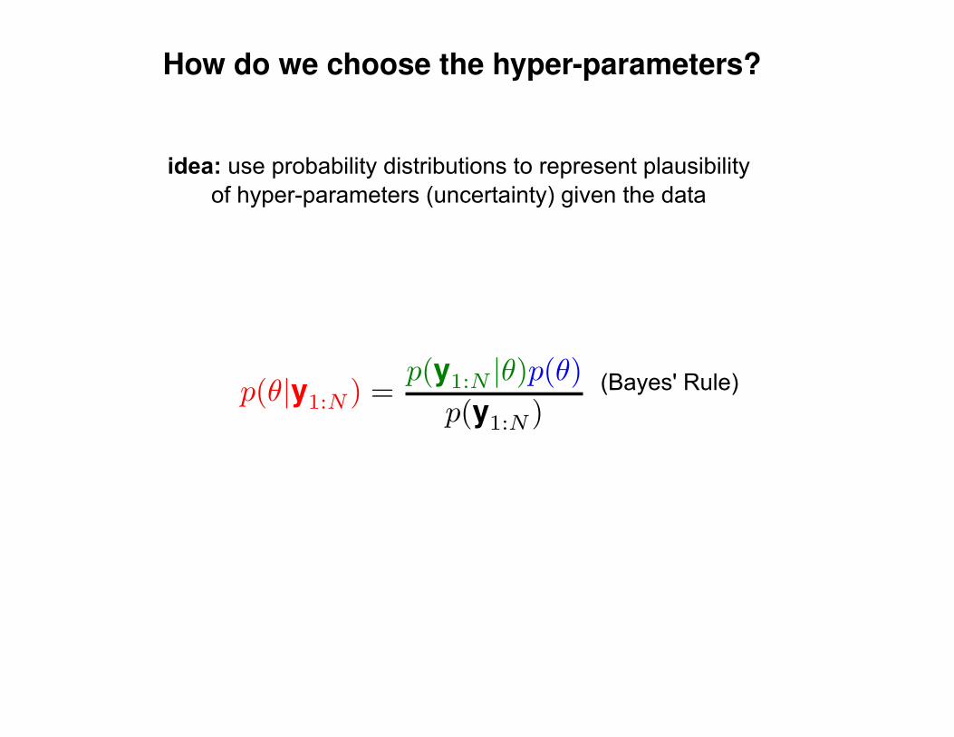
How do we choose the hyper-parameters?
(Bayes' Rule)
idea: use probability distributions to represent plausibility of hyper-parameters (uncertainty) given the data
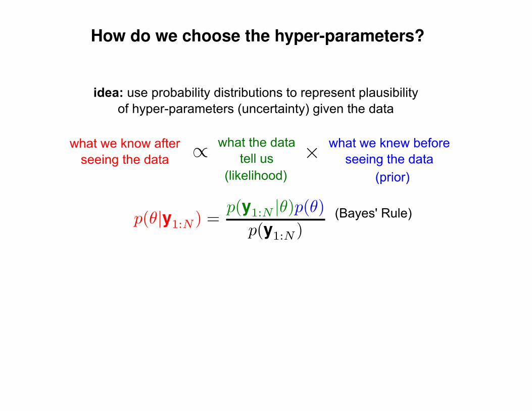
How do we choose the hyper-parameters?
what we know afterseeing the data
what we knew beforeseeing the data
what the datatell us
(Bayes' Rule)
(likelihood) (prior)
idea: use probability distributions to represent plausibility of hyper-parameters (uncertainty) given the data
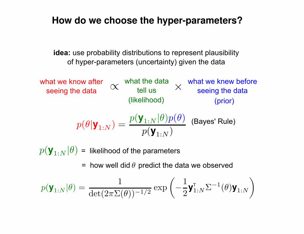
How do we choose the hyper-parameters?
what we know afterseeing the data
what we knew beforeseeing the data
what the datatell us
= how well did predict the data we observed
(Bayes' Rule)
= likelihood of the parameters
(likelihood) (prior)
idea: use probability distributions to represent plausibility of hyper-parameters (uncertainty) given the data
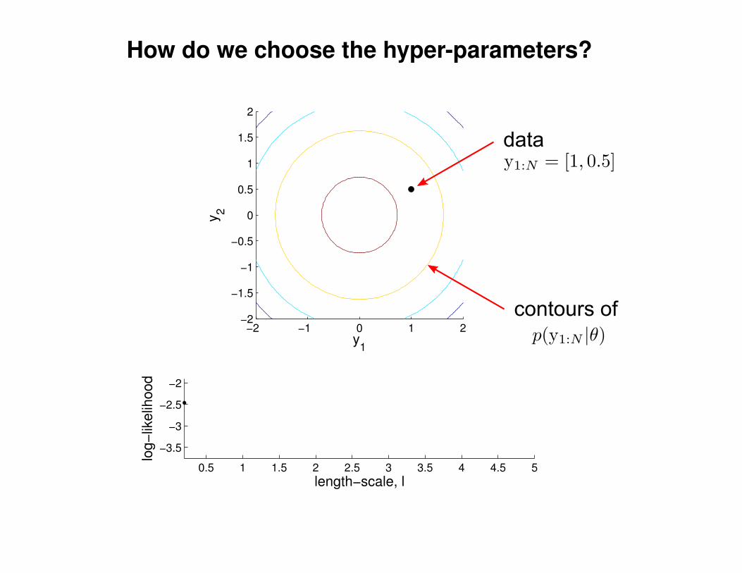
How do we choose the hyper-parameters?
−2 −1 0 1 2−2
−1.5
−1
−0.5
0
0.5
1
1.5
2
y1
y 2
0.5 1 1.5 2 2.5 3 3.5 4 4.5 5
−3.5
−3
−2.5
−2
length−scale, l
log−
likel
ihoo
ddata
contours of
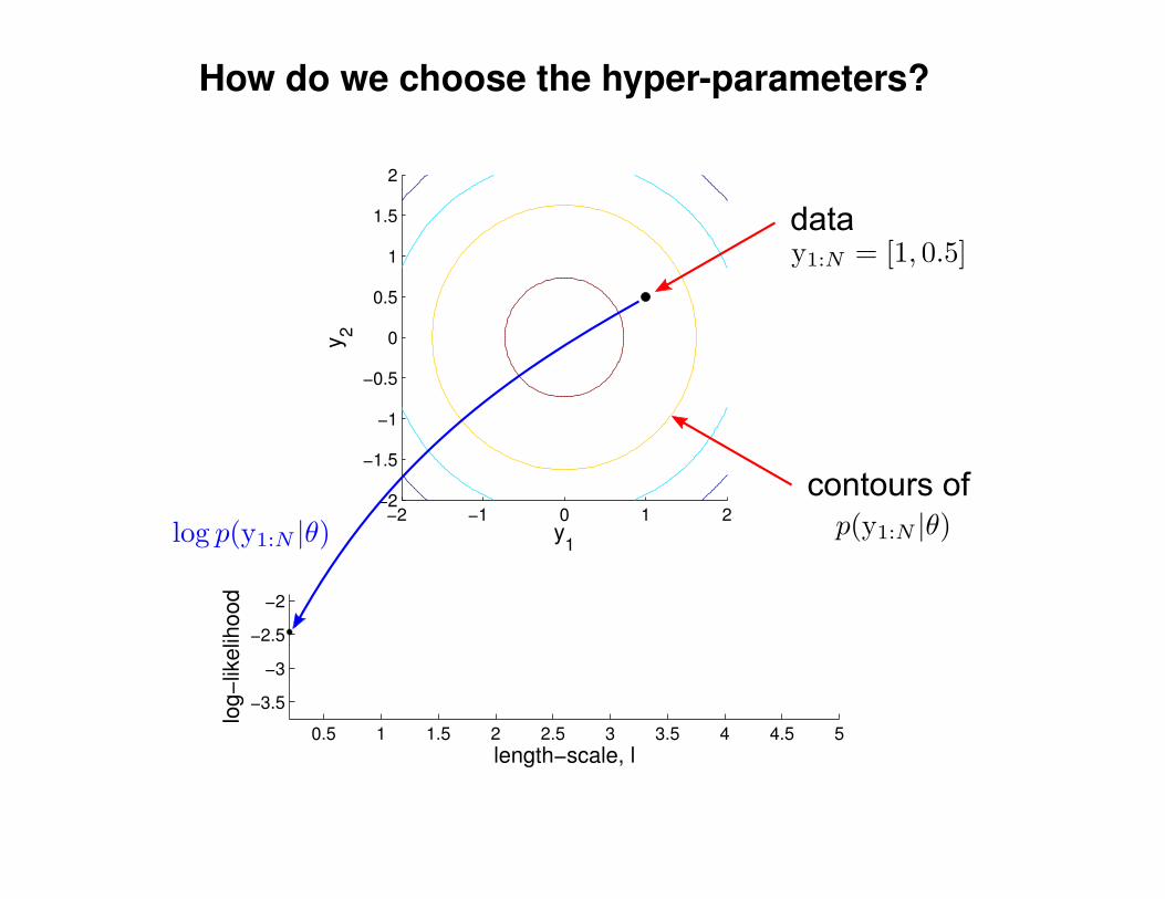
How do we choose the hyper-parameters?
−2 −1 0 1 2−2
−1.5
−1
−0.5
0
0.5
1
1.5
2
y1
y 2
0.5 1 1.5 2 2.5 3 3.5 4 4.5 5
−3.5
−3
−2.5
−2
length−scale, l
log−
likel
ihoo
ddata
contours of

How do we choose the hyper-parameters?
−2 −1 0 1 2−2
−1.5
−1
−0.5
0
0.5
1
1.5
2
y1
y2
0.5 1 1.5 2 2.5 3 3.5 4 4.5 5
−3.5
−3
−2.5
−2
length−scale, l
log
−lik
elih
oo
d
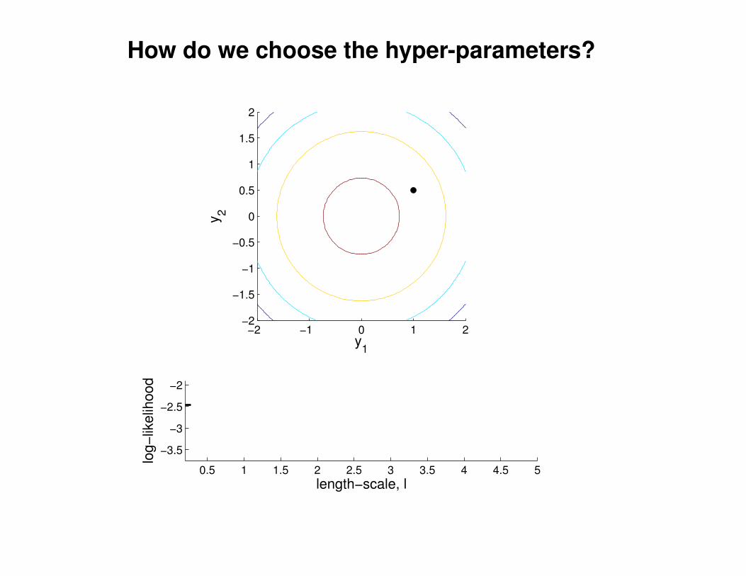
How do we choose the hyper-parameters?
−2 −1 0 1 2−2
−1.5
−1
−0.5
0
0.5
1
1.5
2
y1
y2
0.5 1 1.5 2 2.5 3 3.5 4 4.5 5
−3.5
−3
−2.5
−2
length−scale, l
log
−lik
elih
oo
d
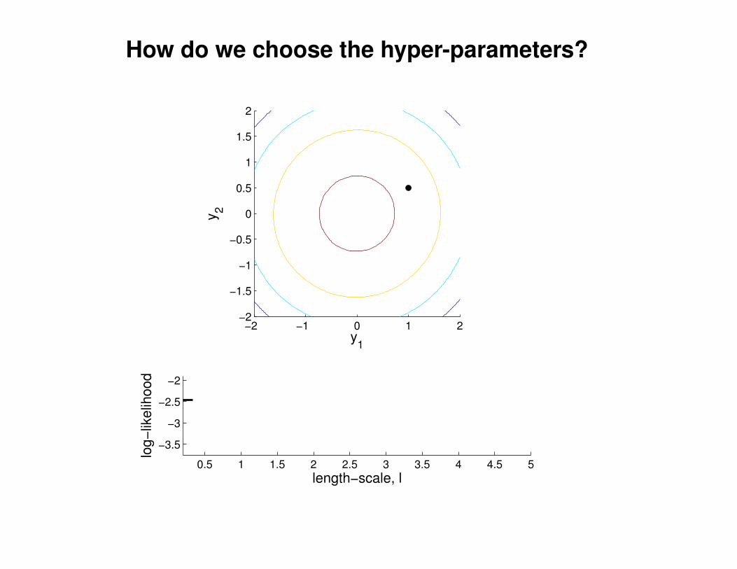
How do we choose the hyper-parameters?
−2 −1 0 1 2−2
−1.5
−1
−0.5
0
0.5
1
1.5
2
y1
y2
0.5 1 1.5 2 2.5 3 3.5 4 4.5 5
−3.5
−3
−2.5
−2
length−scale, l
log
−lik
elih
oo
d

How do we choose the hyper-parameters?
−2 −1 0 1 2−2
−1.5
−1
−0.5
0
0.5
1
1.5
2
y1
y2
0.5 1 1.5 2 2.5 3 3.5 4 4.5 5
−3.5
−3
−2.5
−2
length−scale, l
log
−lik
elih
oo
d
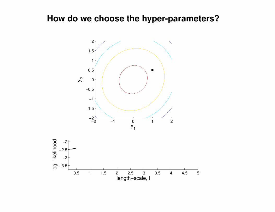
How do we choose the hyper-parameters?
−2 −1 0 1 2−2
−1.5
−1
−0.5
0
0.5
1
1.5
2
y1
y2
0.5 1 1.5 2 2.5 3 3.5 4 4.5 5
−3.5
−3
−2.5
−2
length−scale, l
log
−lik
elih
oo
d
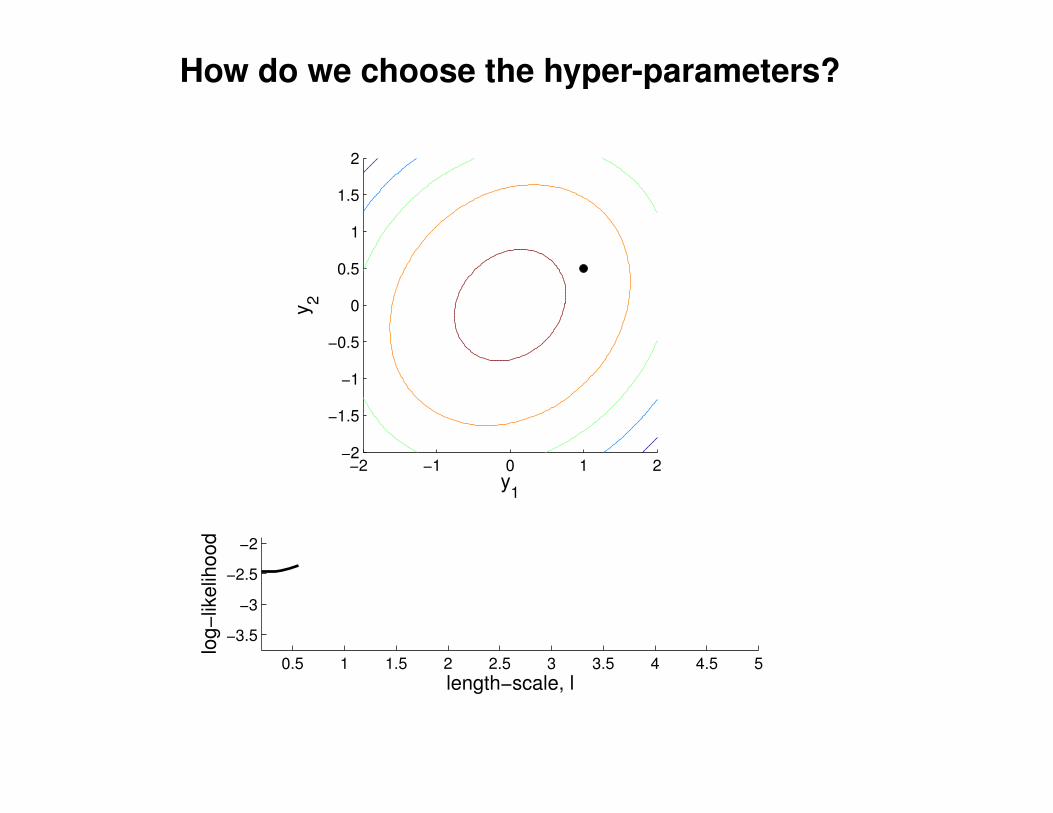
How do we choose the hyper-parameters?
−2 −1 0 1 2−2
−1.5
−1
−0.5
0
0.5
1
1.5
2
y1
y2
0.5 1 1.5 2 2.5 3 3.5 4 4.5 5
−3.5
−3
−2.5
−2
length−scale, l
log
−lik
elih
oo
d
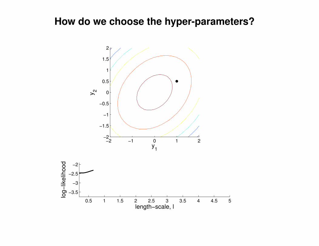
How do we choose the hyper-parameters?
−2 −1 0 1 2−2
−1.5
−1
−0.5
0
0.5
1
1.5
2
y1
y2
0.5 1 1.5 2 2.5 3 3.5 4 4.5 5
−3.5
−3
−2.5
−2
length−scale, l
log
−lik
elih
oo
d
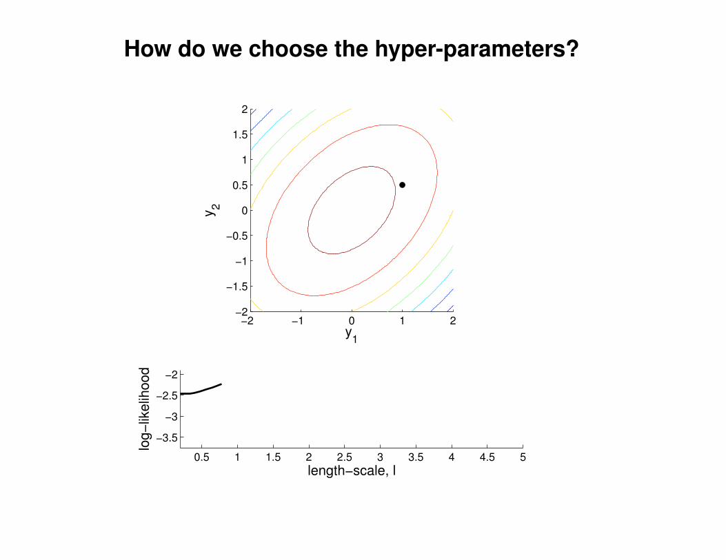
How do we choose the hyper-parameters?
−2 −1 0 1 2−2
−1.5
−1
−0.5
0
0.5
1
1.5
2
y1
y2
0.5 1 1.5 2 2.5 3 3.5 4 4.5 5
−3.5
−3
−2.5
−2
length−scale, l
log
−lik
elih
oo
d
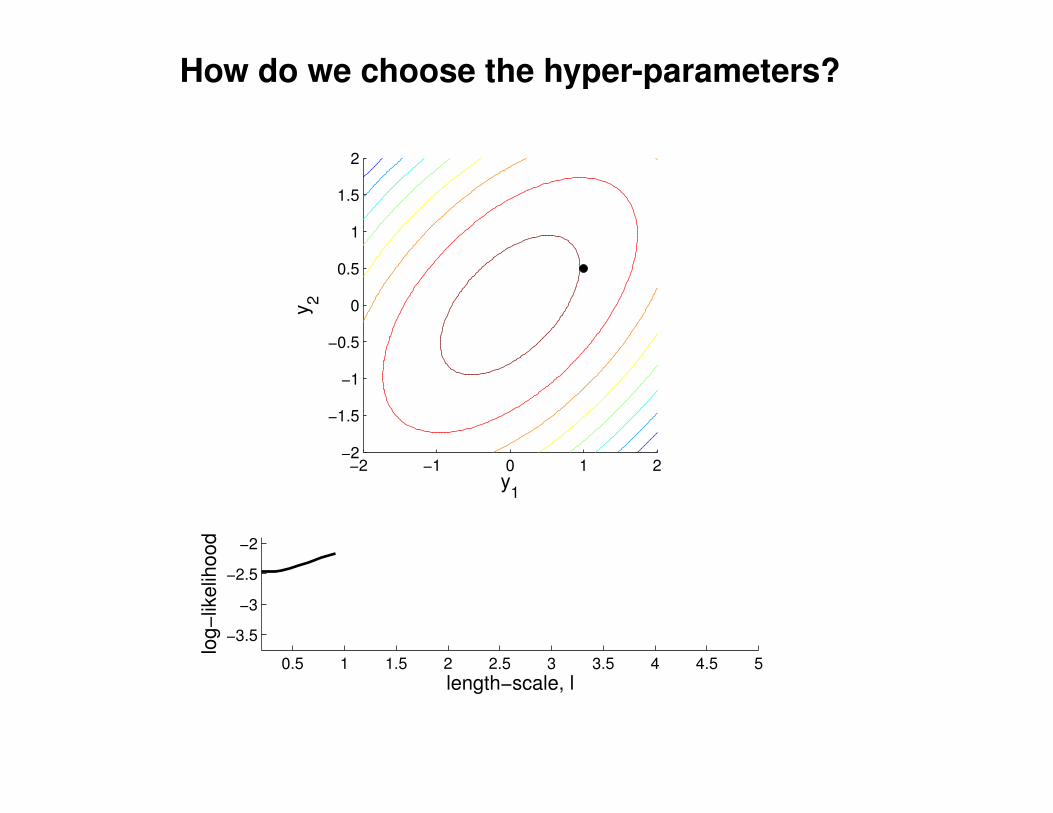
How do we choose the hyper-parameters?
−2 −1 0 1 2−2
−1.5
−1
−0.5
0
0.5
1
1.5
2
y1
y2
0.5 1 1.5 2 2.5 3 3.5 4 4.5 5
−3.5
−3
−2.5
−2
length−scale, l
log
−lik
elih
oo
d
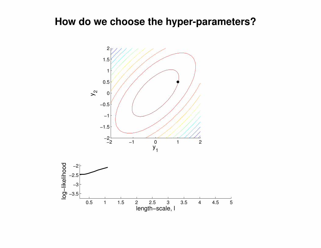
How do we choose the hyper-parameters?
−2 −1 0 1 2−2
−1.5
−1
−0.5
0
0.5
1
1.5
2
y1
y2
0.5 1 1.5 2 2.5 3 3.5 4 4.5 5
−3.5
−3
−2.5
−2
length−scale, l
log
−lik
elih
oo
d
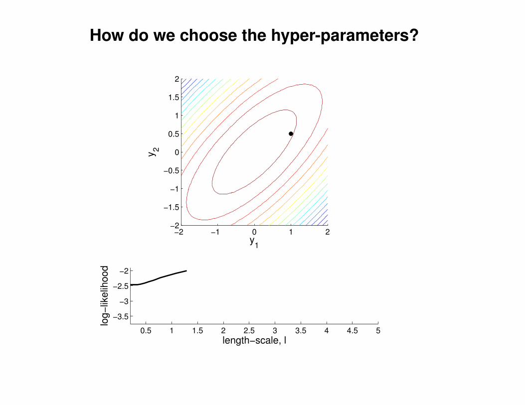
How do we choose the hyper-parameters?
−2 −1 0 1 2−2
−1.5
−1
−0.5
0
0.5
1
1.5
2
y1
y2
0.5 1 1.5 2 2.5 3 3.5 4 4.5 5
−3.5
−3
−2.5
−2
length−scale, l
log
−lik
elih
oo
d

How do we choose the hyper-parameters?
−2 −1 0 1 2−2
−1.5
−1
−0.5
0
0.5
1
1.5
2
y1
y2
0.5 1 1.5 2 2.5 3 3.5 4 4.5 5
−3.5
−3
−2.5
−2
length−scale, l
log
−lik
elih
oo
d
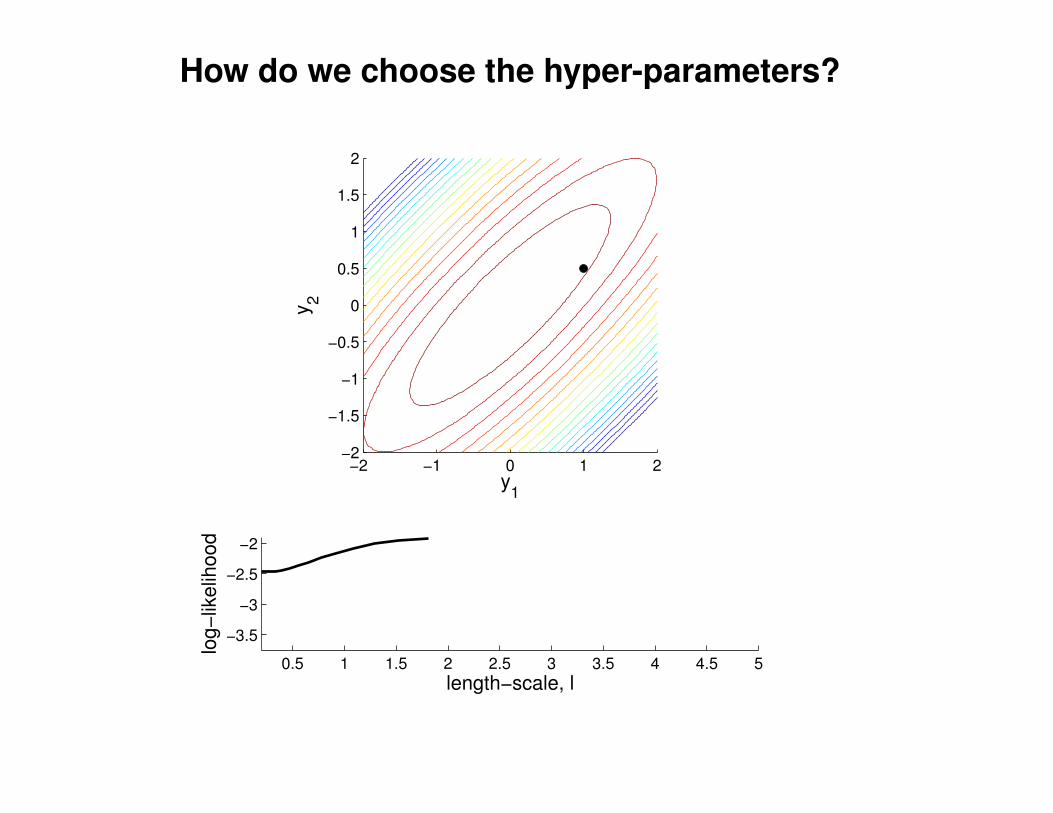
How do we choose the hyper-parameters?
−2 −1 0 1 2−2
−1.5
−1
−0.5
0
0.5
1
1.5
2
y1
y2
0.5 1 1.5 2 2.5 3 3.5 4 4.5 5
−3.5
−3
−2.5
−2
length−scale, l
log
−lik
elih
oo
d
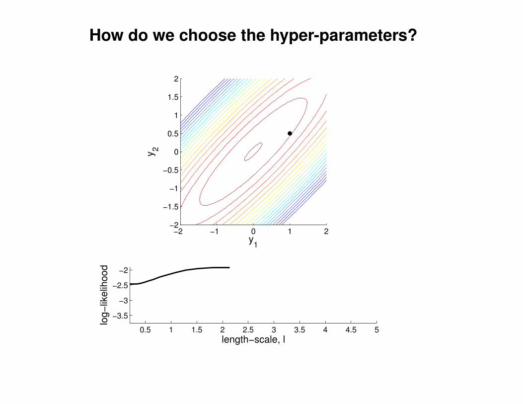
How do we choose the hyper-parameters?
−2 −1 0 1 2−2
−1.5
−1
−0.5
0
0.5
1
1.5
2
y1
y2
0.5 1 1.5 2 2.5 3 3.5 4 4.5 5
−3.5
−3
−2.5
−2
length−scale, l
log
−lik
elih
oo
d
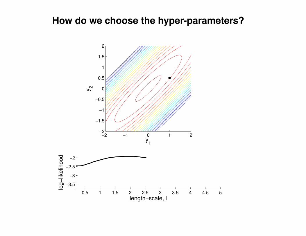
How do we choose the hyper-parameters?
−2 −1 0 1 2−2
−1.5
−1
−0.5
0
0.5
1
1.5
2
y1
y2
0.5 1 1.5 2 2.5 3 3.5 4 4.5 5
−3.5
−3
−2.5
−2
length−scale, l
log
−lik
elih
oo
d
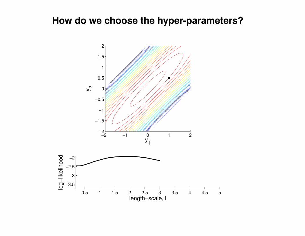
How do we choose the hyper-parameters?
−2 −1 0 1 2−2
−1.5
−1
−0.5
0
0.5
1
1.5
2
y1
y2
0.5 1 1.5 2 2.5 3 3.5 4 4.5 5
−3.5
−3
−2.5
−2
length−scale, l
log
−lik
elih
oo
d
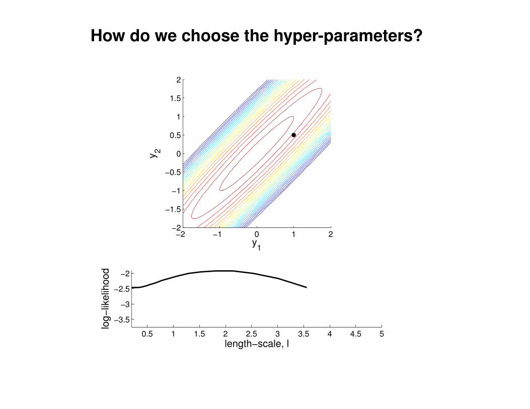
How do we choose the hyper-parameters?
−2 −1 0 1 2−2
−1.5
−1
−0.5
0
0.5
1
1.5
2
y1
y2
0.5 1 1.5 2 2.5 3 3.5 4 4.5 5
−3.5
−3
−2.5
−2
length−scale, l
log
−lik
elih
oo
d
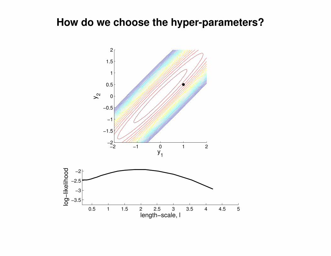
How do we choose the hyper-parameters?
−2 −1 0 1 2−2
−1.5
−1
−0.5
0
0.5
1
1.5
2
y1
y2
0.5 1 1.5 2 2.5 3 3.5 4 4.5 5
−3.5
−3
−2.5
−2
length−scale, l
log
−lik
elih
oo
d
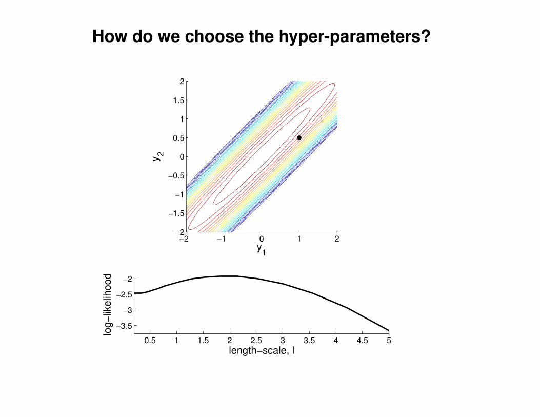
How do we choose the hyper-parameters?
−2 −1 0 1 2−2
−1.5
−1
−0.5
0
0.5
1
1.5
2
y1
y2
0.5 1 1.5 2 2.5 3 3.5 4 4.5 5
−3.5
−3
−2.5
−2
length−scale, l
log
−lik
elih
oo
d
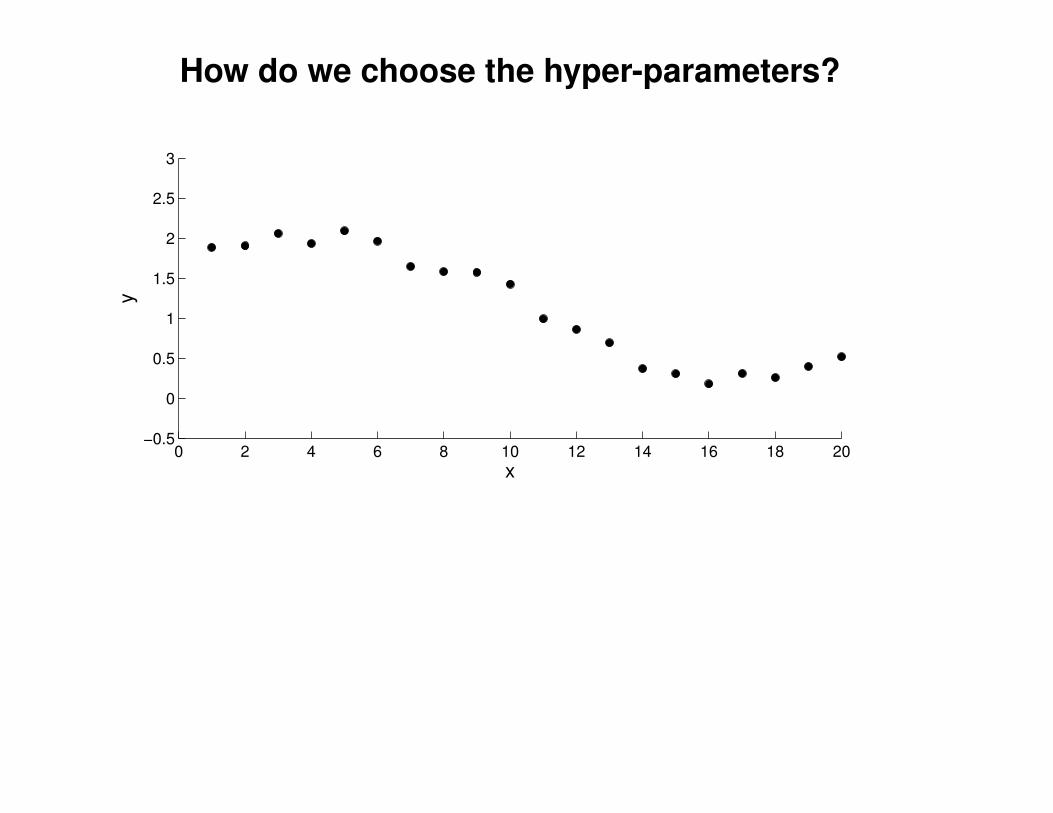
How do we choose the hyper-parameters?
0 2 4 6 8 10 12 14 16 18 20−0.5
0
0.5
1
1.5
2
2.5
3
x
y
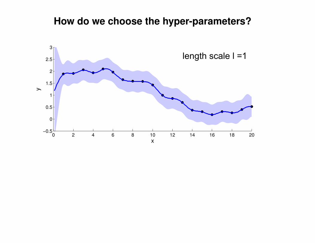
How do we choose the hyper-parameters?
0 2 4 6 8 10 12 14 16 18 20−0.5
0
0.5
1
1.5
2
2.5
3
x
y
length scale l =1
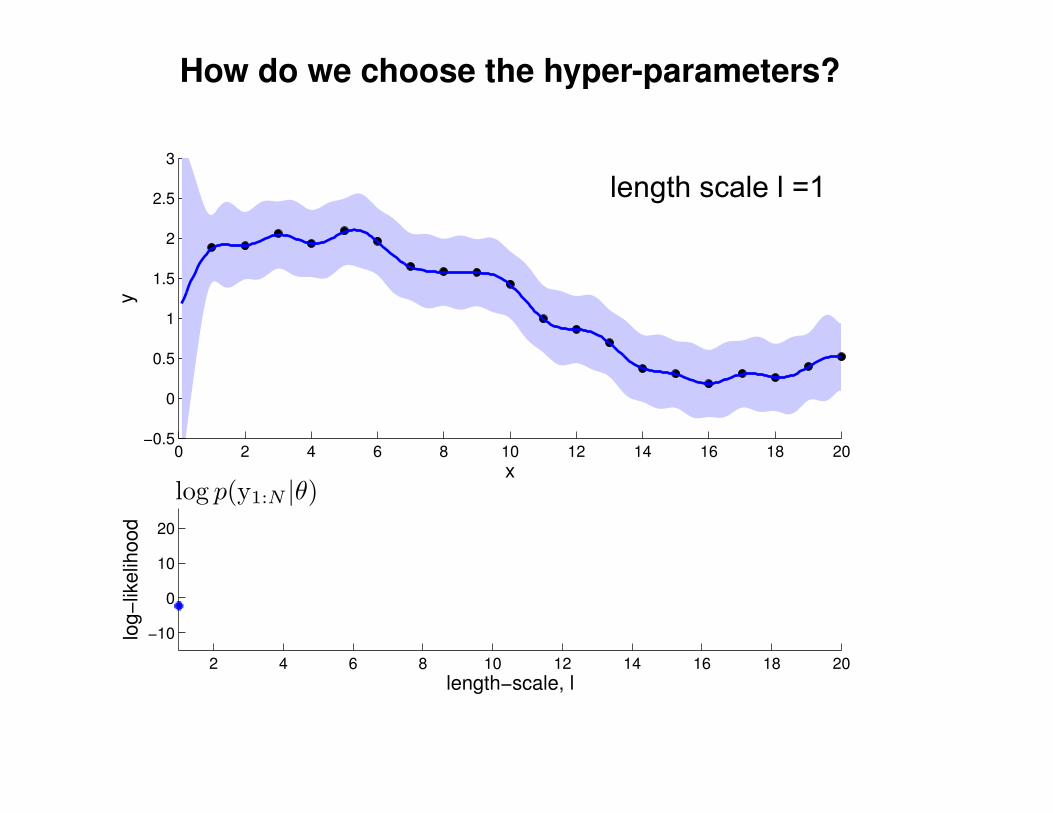
How do we choose the hyper-parameters?
0 2 4 6 8 10 12 14 16 18 20−0.5
0
0.5
1
1.5
2
2.5
3
x
y
2 4 6 8 10 12 14 16 18 20
−10
0
10
20
length−scale, l
log−
likel
ihoo
d
length scale l =1
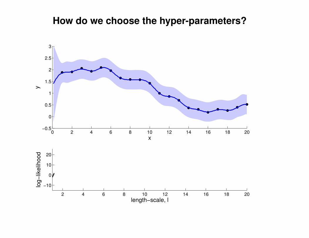
How do we choose the hyper-parameters?
0 2 4 6 8 10 12 14 16 18 20−0.5
0
0.5
1
1.5
2
2.5
3
x
y
2 4 6 8 10 12 14 16 18 20
−10
0
10
20
length−scale, l
log
−lik
elih
oo
d

How do we choose the hyper-parameters?
0 2 4 6 8 10 12 14 16 18 20−0.5
0
0.5
1
1.5
2
2.5
3
x
y
2 4 6 8 10 12 14 16 18 20
−10
0
10
20
length−scale, l
log
−lik
elih
oo
d
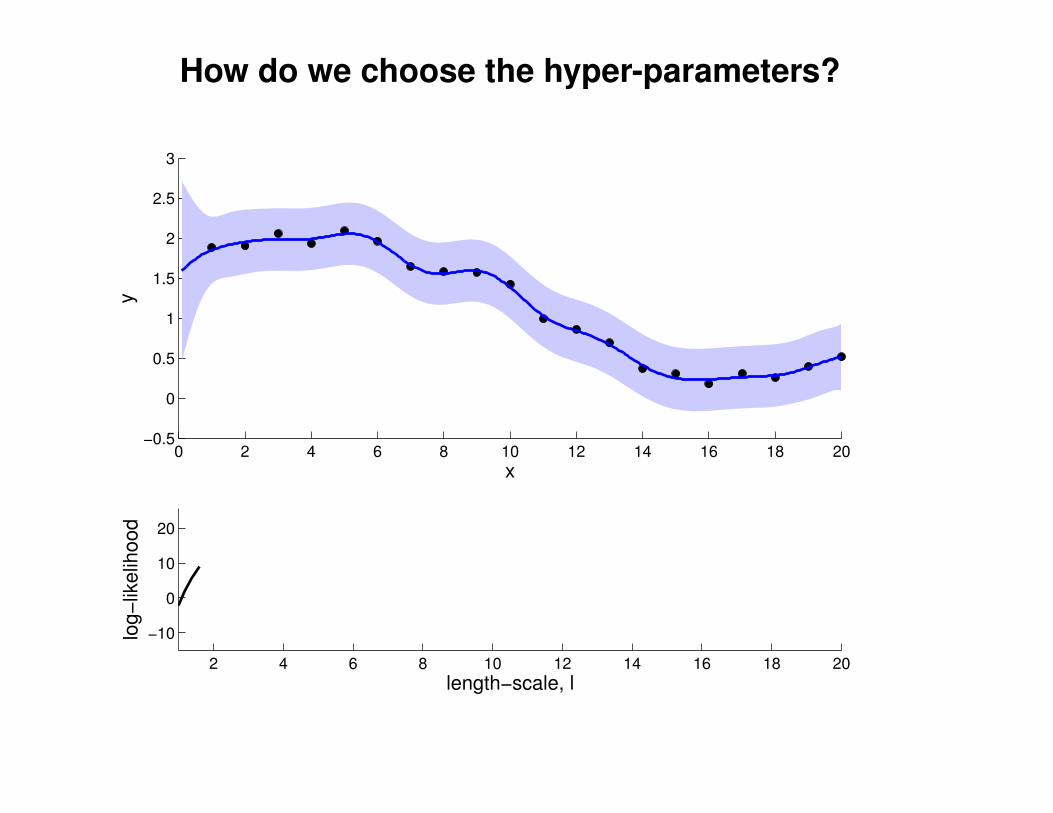
How do we choose the hyper-parameters?
0 2 4 6 8 10 12 14 16 18 20−0.5
0
0.5
1
1.5
2
2.5
3
x
y
2 4 6 8 10 12 14 16 18 20
−10
0
10
20
length−scale, l
log
−lik
elih
oo
d
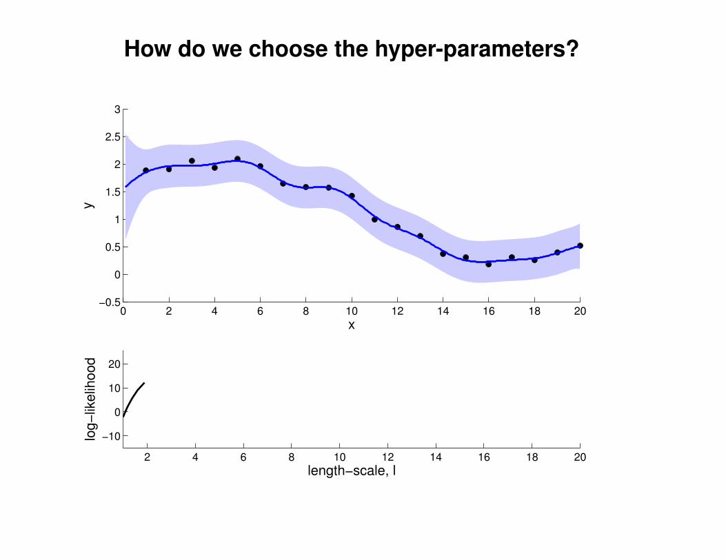
How do we choose the hyper-parameters?
0 2 4 6 8 10 12 14 16 18 20−0.5
0
0.5
1
1.5
2
2.5
3
x
y
2 4 6 8 10 12 14 16 18 20
−10
0
10
20
length−scale, l
log
−lik
elih
oo
d

How do we choose the hyper-parameters?
0 2 4 6 8 10 12 14 16 18 20−0.5
0
0.5
1
1.5
2
2.5
3
x
y
2 4 6 8 10 12 14 16 18 20
−10
0
10
20
length−scale, l
log
−lik
elih
oo
d

How do we choose the hyper-parameters?
0 2 4 6 8 10 12 14 16 18 20−0.5
0
0.5
1
1.5
2
2.5
3
x
y
2 4 6 8 10 12 14 16 18 20
−10
0
10
20
length−scale, l
log
−lik
elih
oo
d

How do we choose the hyper-parameters?
0 2 4 6 8 10 12 14 16 18 20−0.5
0
0.5
1
1.5
2
2.5
3
x
y
2 4 6 8 10 12 14 16 18 20
−10
0
10
20
length−scale, l
log
−lik
elih
oo
d

How do we choose the hyper-parameters?
0 2 4 6 8 10 12 14 16 18 20−0.5
0
0.5
1
1.5
2
2.5
3
x
y
2 4 6 8 10 12 14 16 18 20
−10
0
10
20
length−scale, l
log
−lik
elih
oo
d

How do we choose the hyper-parameters?
0 2 4 6 8 10 12 14 16 18 20−0.5
0
0.5
1
1.5
2
2.5
3
x
y
2 4 6 8 10 12 14 16 18 20
−10
0
10
20
length−scale, l
log
−lik
elih
oo
d

How do we choose the hyper-parameters?
0 2 4 6 8 10 12 14 16 18 20−0.5
0
0.5
1
1.5
2
2.5
3
x
y
2 4 6 8 10 12 14 16 18 20
−10
0
10
20
length−scale, l
log
−lik
elih
oo
d
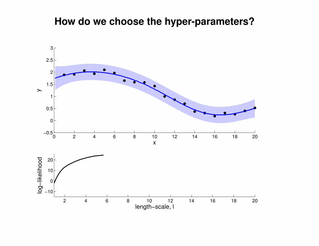
How do we choose the hyper-parameters?
0 2 4 6 8 10 12 14 16 18 20−0.5
0
0.5
1
1.5
2
2.5
3
x
y
2 4 6 8 10 12 14 16 18 20
−10
0
10
20
length−scale, l
log
−lik
elih
oo
d

How do we choose the hyper-parameters?
0 2 4 6 8 10 12 14 16 18 20−0.5
0
0.5
1
1.5
2
2.5
3
x
y
2 4 6 8 10 12 14 16 18 20
−10
0
10
20
length−scale, l
log
−lik
elih
oo
d
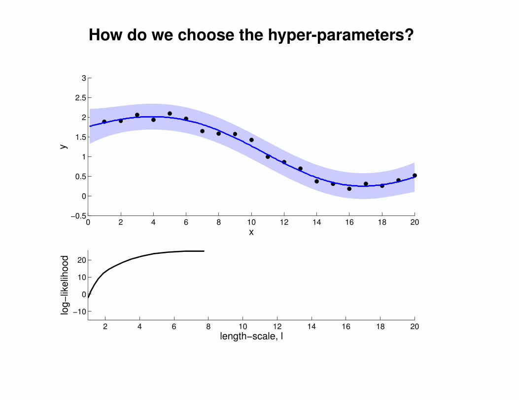
How do we choose the hyper-parameters?
0 2 4 6 8 10 12 14 16 18 20−0.5
0
0.5
1
1.5
2
2.5
3
x
y
2 4 6 8 10 12 14 16 18 20
−10
0
10
20
length−scale, l
log
−lik
elih
oo
d
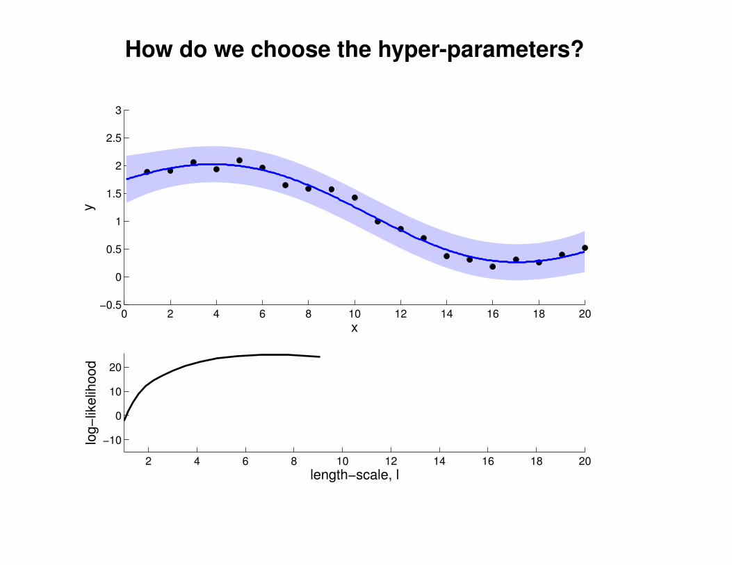
How do we choose the hyper-parameters?
0 2 4 6 8 10 12 14 16 18 20−0.5
0
0.5
1
1.5
2
2.5
3
x
y
2 4 6 8 10 12 14 16 18 20
−10
0
10
20
length−scale, l
log
−lik
elih
oo
d

How do we choose the hyper-parameters?
0 2 4 6 8 10 12 14 16 18 20−0.5
0
0.5
1
1.5
2
2.5
3
x
y
2 4 6 8 10 12 14 16 18 20
−10
0
10
20
length−scale, l
log
−lik
elih
oo
d
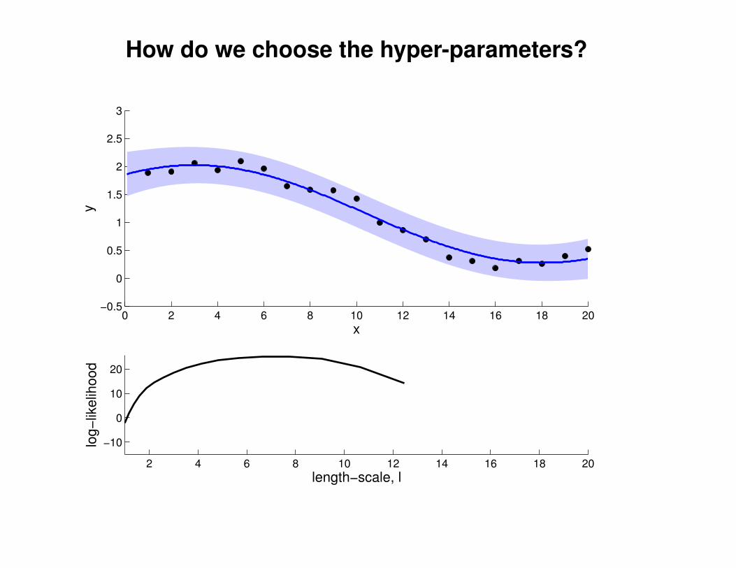
How do we choose the hyper-parameters?
0 2 4 6 8 10 12 14 16 18 20−0.5
0
0.5
1
1.5
2
2.5
3
x
y
2 4 6 8 10 12 14 16 18 20
−10
0
10
20
length−scale, l
log
−lik
elih
oo
d
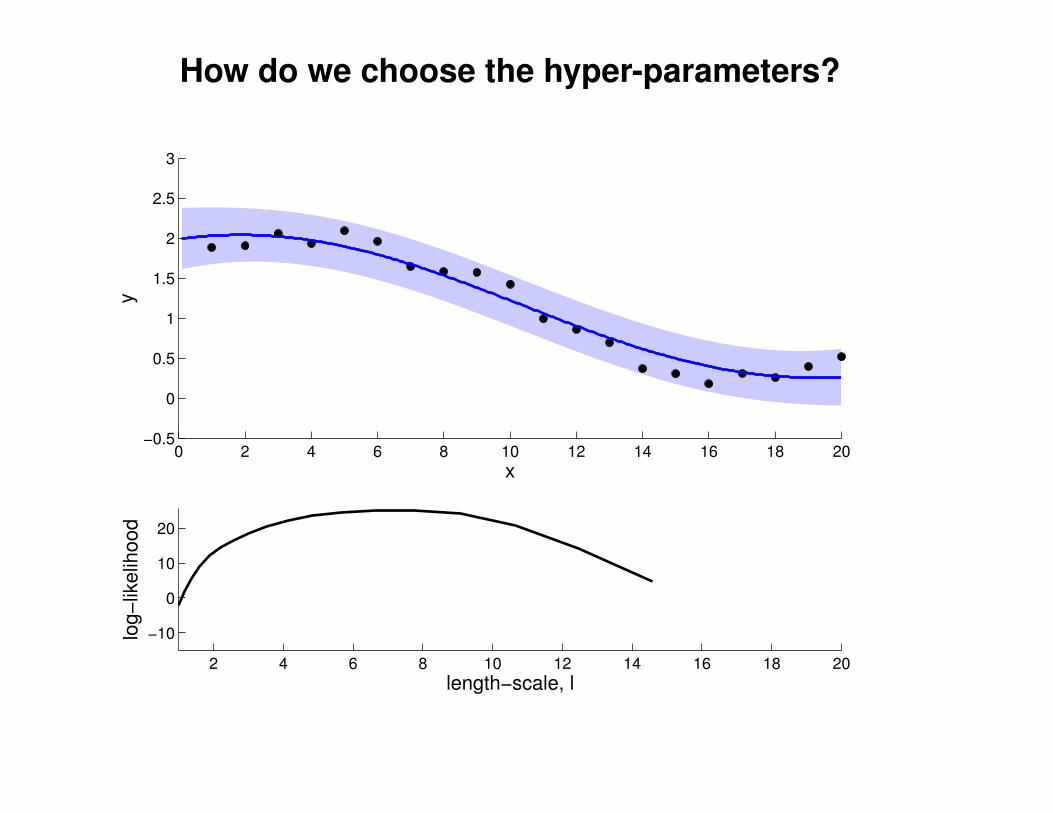
How do we choose the hyper-parameters?
0 2 4 6 8 10 12 14 16 18 20−0.5
0
0.5
1
1.5
2
2.5
3
x
y
2 4 6 8 10 12 14 16 18 20
−10
0
10
20
length−scale, l
log
−lik
elih
oo
d
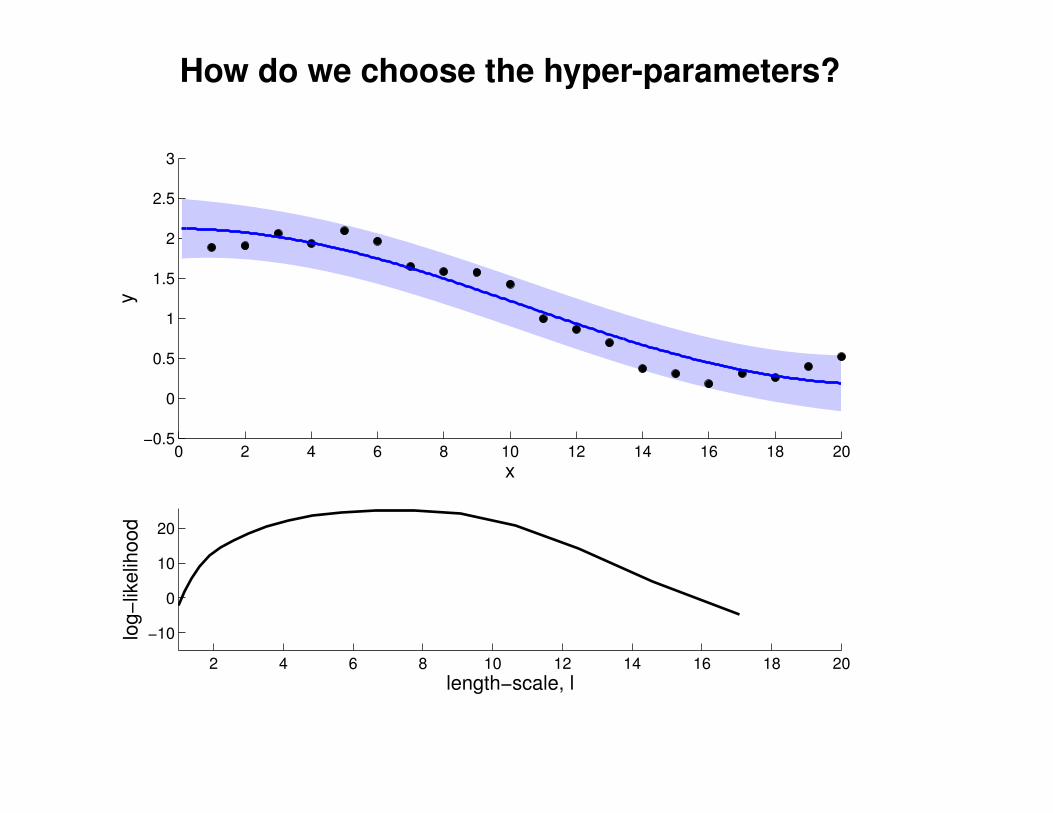
How do we choose the hyper-parameters?
0 2 4 6 8 10 12 14 16 18 20−0.5
0
0.5
1
1.5
2
2.5
3
x
y
2 4 6 8 10 12 14 16 18 20
−10
0
10
20
length−scale, l
log
−lik
elih
oo
d

How do we choose the hyper-parameters?
0 2 4 6 8 10 12 14 16 18 20−0.5
0
0.5
1
1.5
2
2.5
3
x
y
2 4 6 8 10 12 14 16 18 20
−10
0
10
20
length−scale, l
log
−lik
elih
oo
d
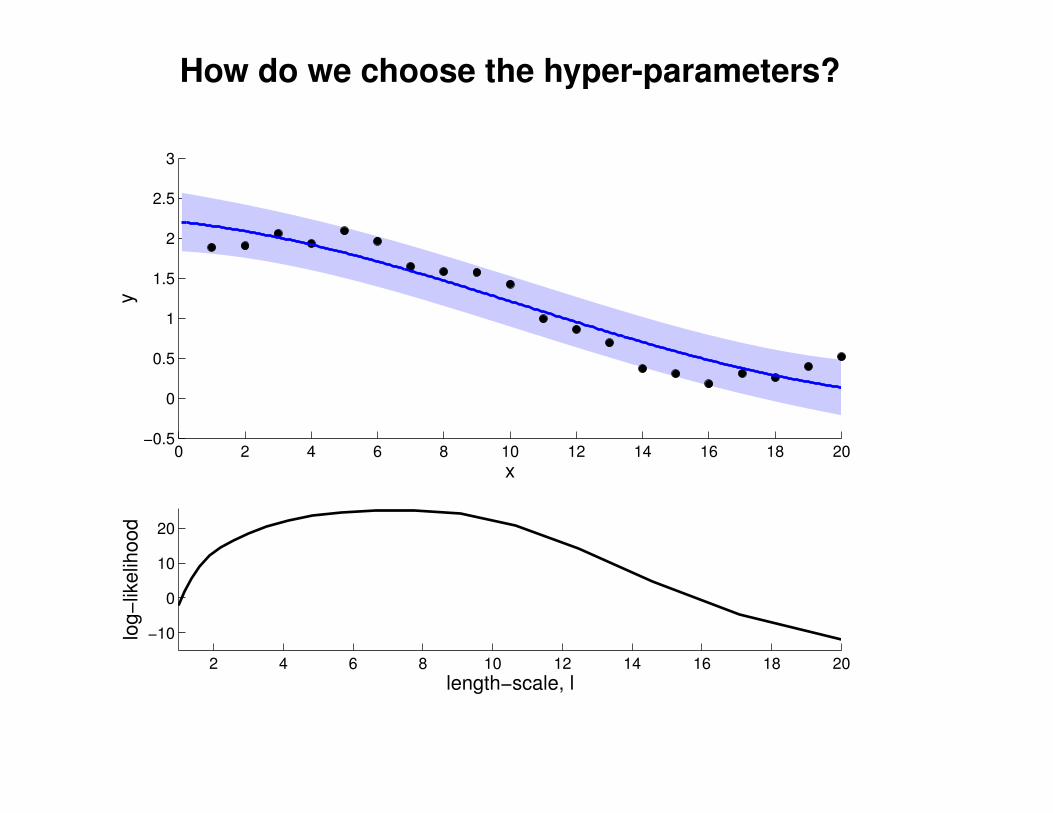
How do we choose the hyper-parameters?
0 2 4 6 8 10 12 14 16 18 20−0.5
0
0.5
1
1.5
2
2.5
3
x
y
2 4 6 8 10 12 14 16 18 20
−10
0
10
20
length−scale, l
log
−lik
elih
oo
d
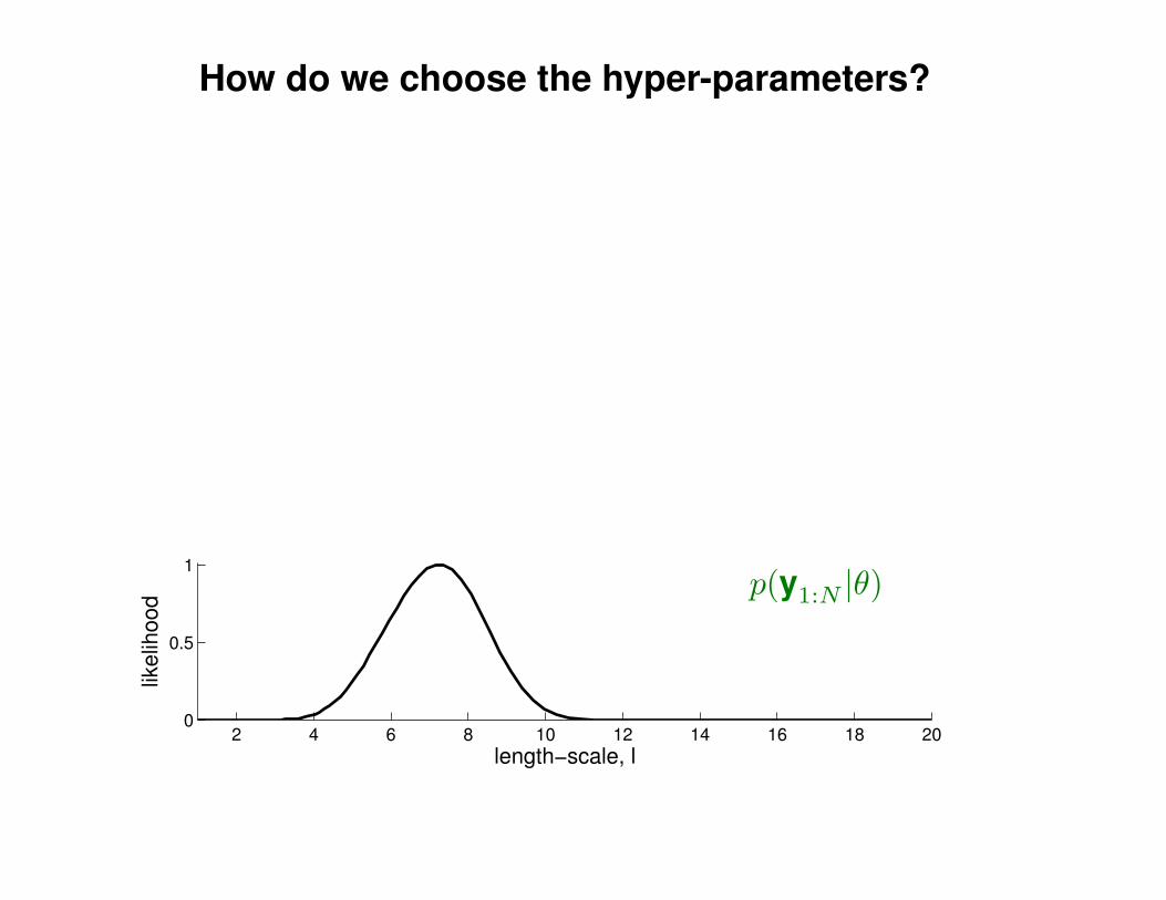
How do we choose the hyper-parameters?
2 4 6 8 10 12 14 16 18 200
0.5
1
length−scale, l
likel
ihoo
d
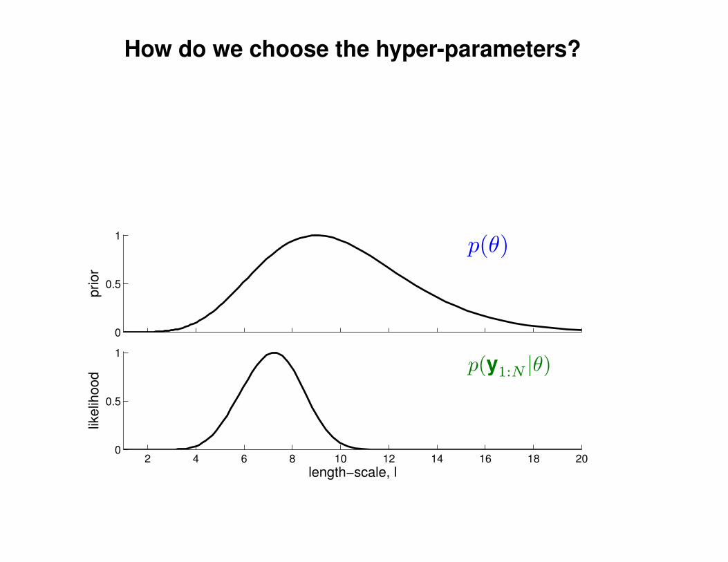
How do we choose the hyper-parameters?
2 4 6 8 10 12 14 16 18 200
0.5
1
length−scale, l
likel
ihoo
d
0
0.5
1
prio
r
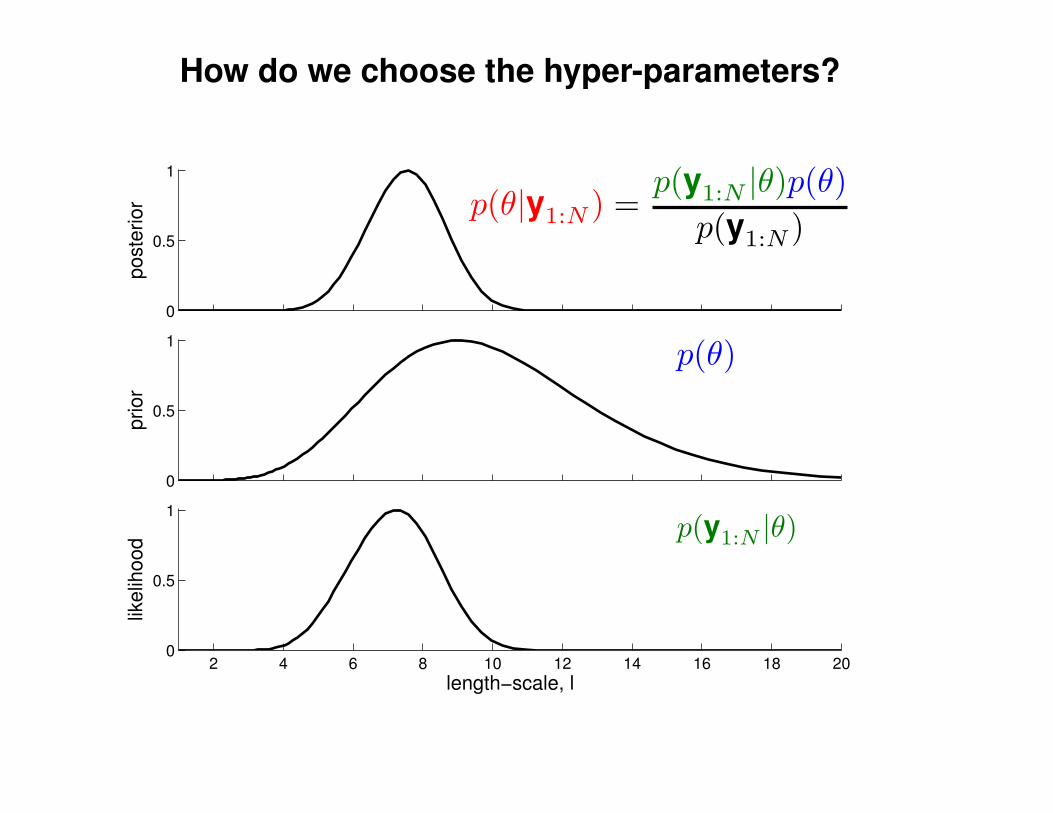
How do we choose the hyper-parameters?
2 4 6 8 10 12 14 16 18 200
0.5
1
length−scale, l
likel
ihoo
d
0
0.5
1
prio
r
0
0.5
1
post
erio
r
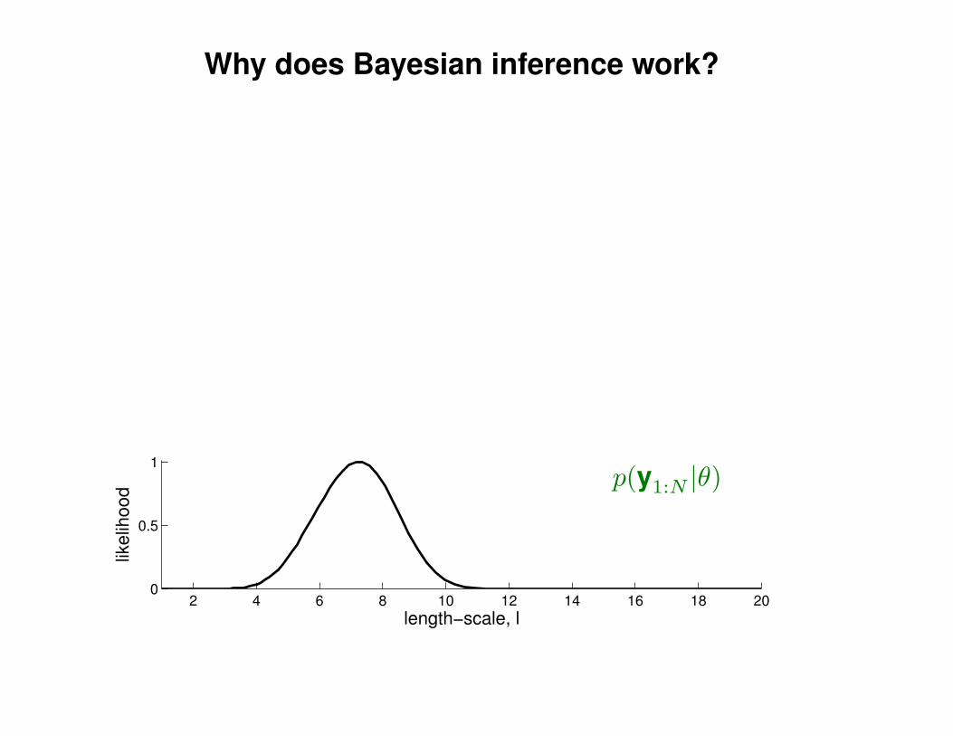
Why does Bayesian inference work?
2 4 6 8 10 12 14 16 18 200
0.5
1
length−scale, l
likel
ihoo
d
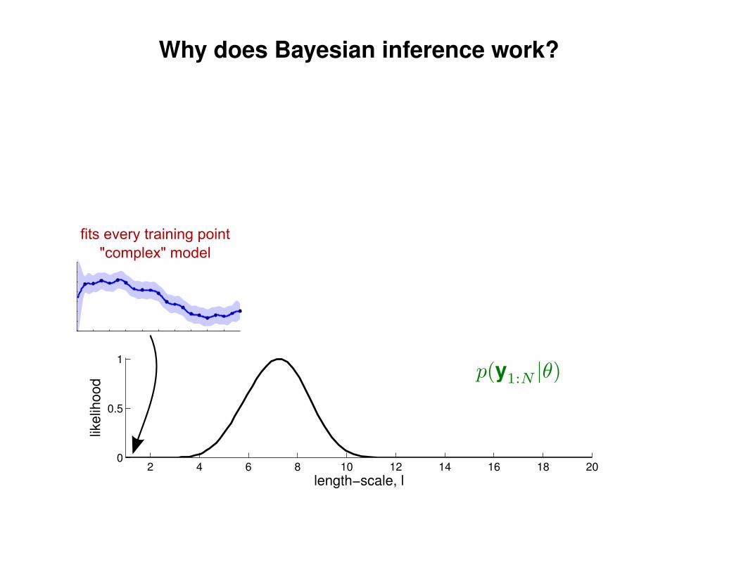
Why does Bayesian inference work?
2 4 6 8 10 12 14 16 18 200
0.5
1
length−scale, l
likel
ihoo
d
fits every training point"complex" model
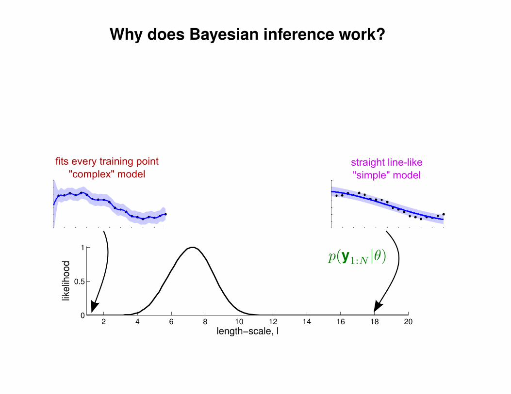
Why does Bayesian inference work?
2 4 6 8 10 12 14 16 18 200
0.5
1
length−scale, l
likel
ihoo
d
fits every training point"complex" model
straight line-like"simple" model
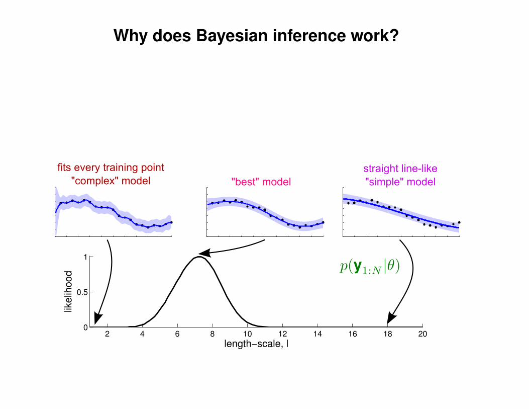
Why does Bayesian inference work?
2 4 6 8 10 12 14 16 18 200
0.5
1
length−scale, l
likel
ihoo
d
fits every training point"complex" model
straight line-like"simple" model"best" model
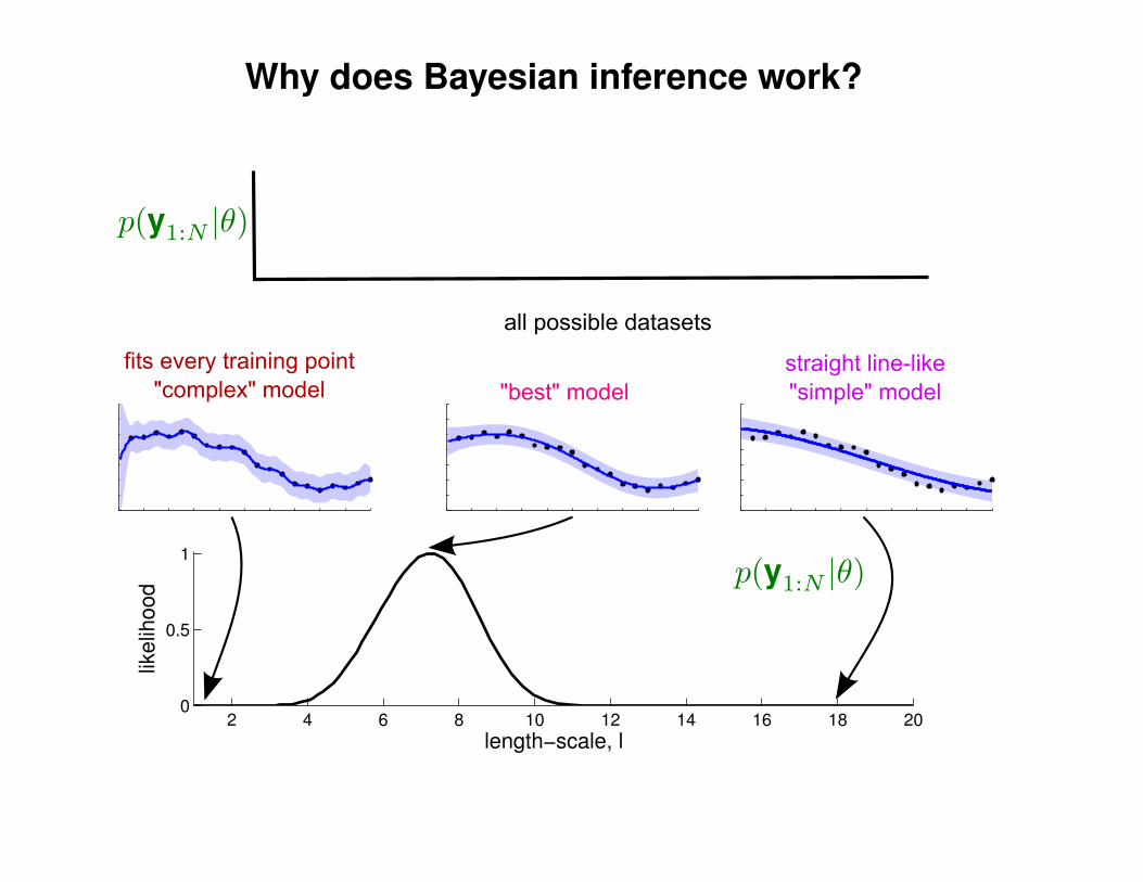
Why does Bayesian inference work?
2 4 6 8 10 12 14 16 18 200
0.5
1
length−scale, l
likel
ihoo
d
fits every training point"complex" model
straight line-like"simple" model
all possible datasets
"best" model
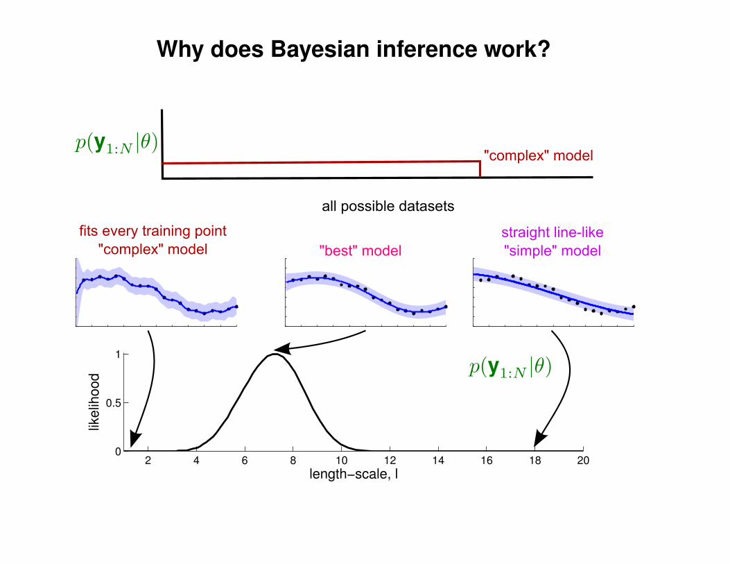
Why does Bayesian inference work?
2 4 6 8 10 12 14 16 18 200
0.5
1
length−scale, l
likel
ihoo
d
fits every training point"complex" model
straight line-like"simple" model
all possible datasets
"best" model
"complex" model
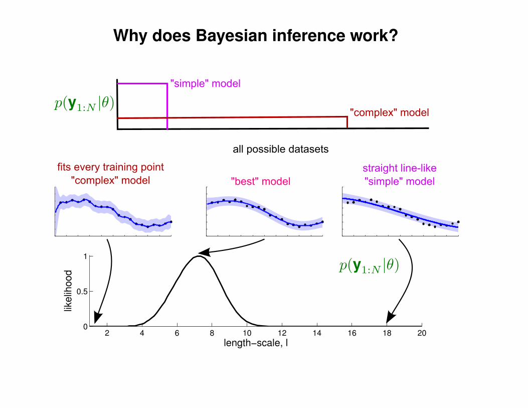
Why does Bayesian inference work?
2 4 6 8 10 12 14 16 18 200
0.5
1
length−scale, l
likel
ihoo
d
fits every training point"complex" model
straight line-like"simple" model
all possible datasets
"best" model
"complex" model
"simple" model
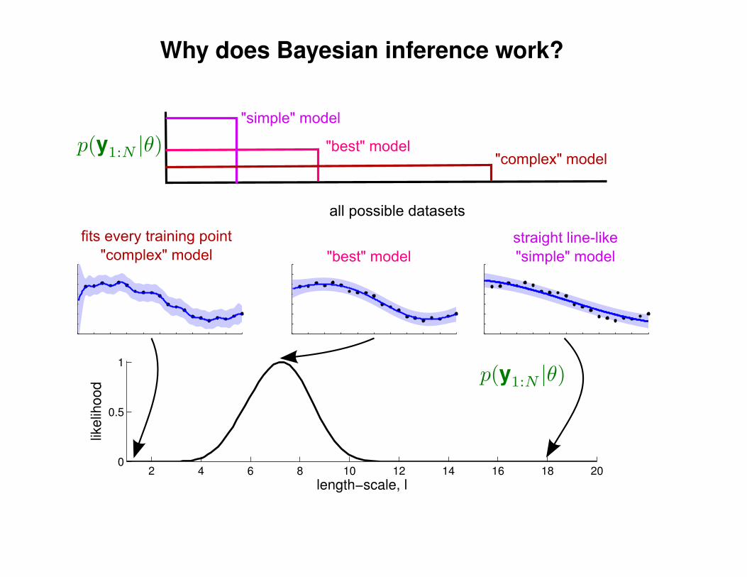
Why does Bayesian inference work?
2 4 6 8 10 12 14 16 18 200
0.5
1
length−scale, l
likel
ihoo
d
fits every training point"complex" model
straight line-like"simple" model
all possible datasets
"best" model
"complex" model"best" model
"simple" model
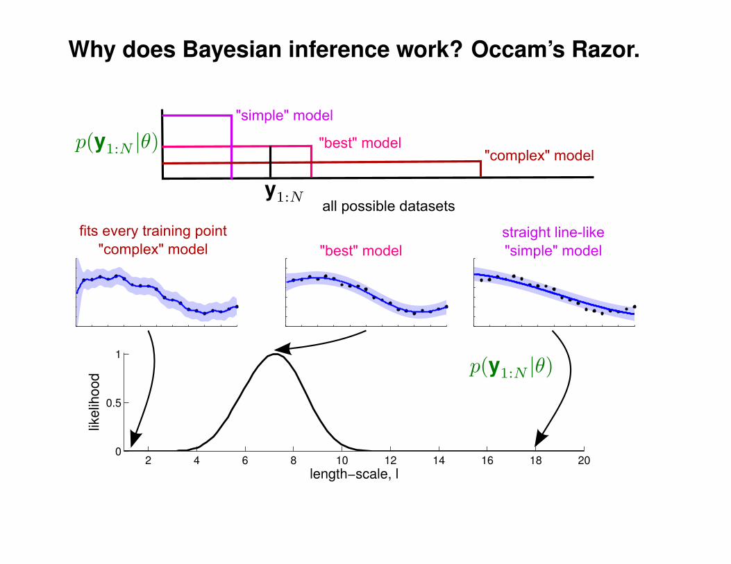
Why does Bayesian inference work? Occam’s Razor.
2 4 6 8 10 12 14 16 18 200
0.5
1
length−scale, l
likel
ihoo
d
fits every training point"complex" model
straight line-like"simple" model
all possible datasets
"best" model
"complex" model"best" model
"simple" model
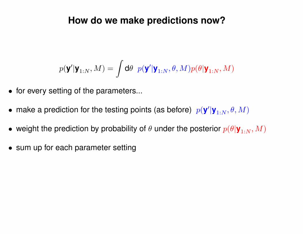
How do we make predictions now?
p(y′|y1:N ,M) =
∫dθ p(y′|y1:N , θ,M)p(θ|y1:N ,M)
• for every setting of the parameters...
• make a prediction for the testing points (as before) p(y′|y1:N , θ,M)
• weight the prediction by probability of θ under the posterior p(θ|y1:N ,M)
• sum up for each parameter setting
Only need two rules for Bayesian computation: product and sum rules
p(x, y) = p(x|y)p(y) = p(y|x)p(x) p(x) =∑
y
p(x, y)
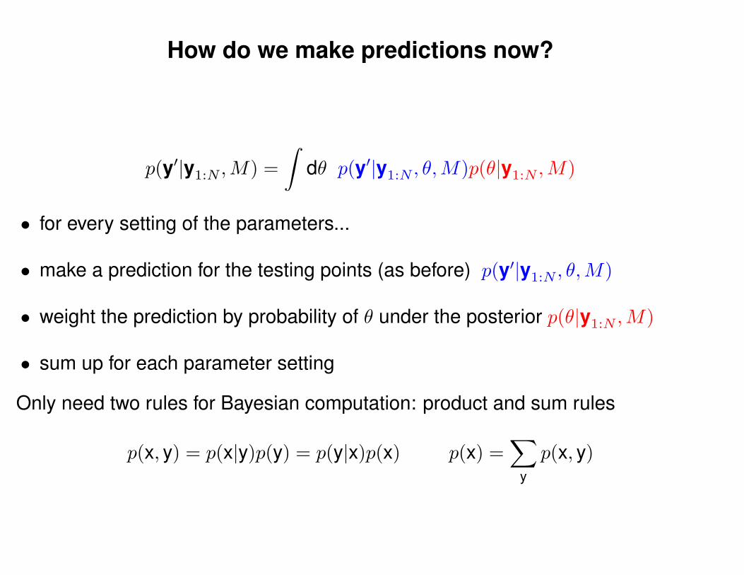
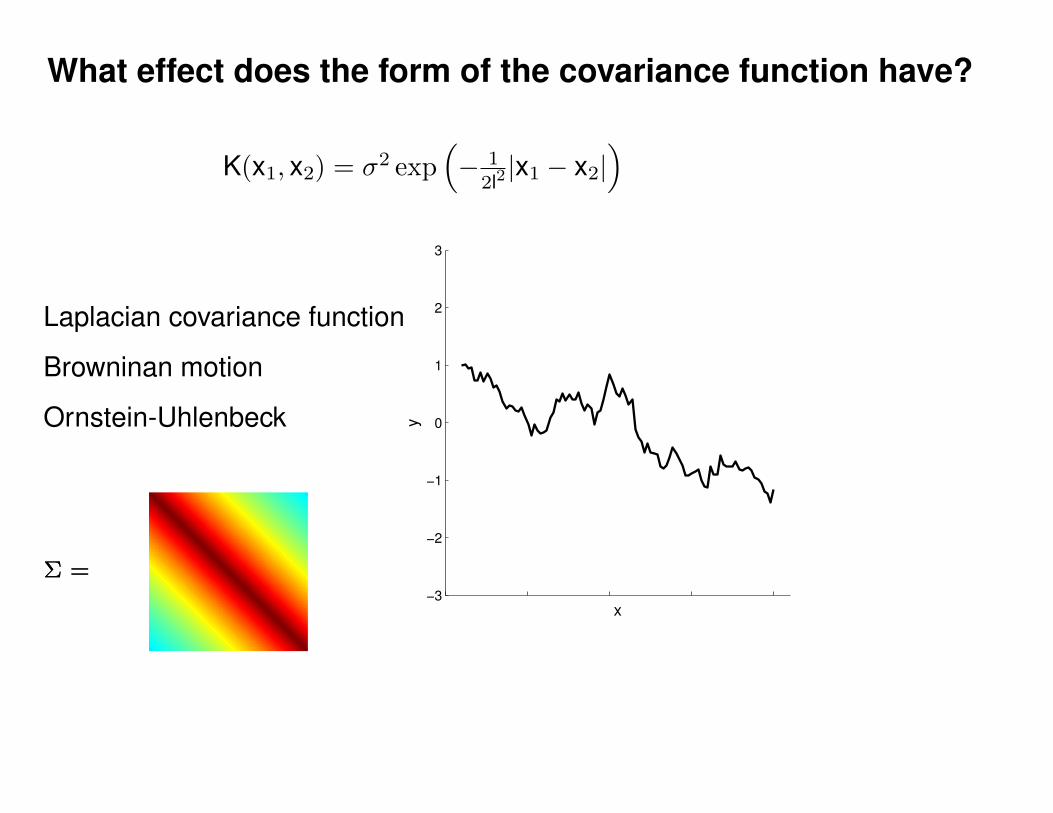
What effect does the form of the covariance function have?
−3
−2
−1
0
1
2
3
x
y
Σ =
Laplacian covariance function
Browninan motion
Ornstein-Uhlenbeck
Σ =
K(x1, x2) = σ2 exp(− 1
2l2|x1 − x2|
)

What effect does the form of the covariance function have?
−3
−2
−1
0
1
2
3
x
y
−3
−2
−1
0
1
2
3
x
y
Σ =
Laplacian covariance function
Browninan motion
Ornstein-Uhlenbeck
K(x1, x2) = σ2 exp(− 1
2l2|x1 − x2|
)

What effect does the form of the covariance function have?
−3
−2
−1
0
1
2
3
x
y
−3
−2
−1
0
1
2
3
x
y
−3
−2
−1
0
1
2
3
x
y
Σ =
Laplacian covariance function
Browninan motion
Ornstein-Uhlenbeck
K(x1, x2) = σ2 exp(− 1
2l2|x1 − x2|
)

What effect does the form of the covariance function have?
−3
−2
−1
0
1
2
3
x
y
−3
−2
−1
0
1
2
3
x
y
−3
−2
−1
0
1
2
3
x
y
−3
−2
−1
0
1
2
3
x
y
Σ =
Laplacian covariance function
Browninan motion
Ornstein-Uhlenbeck
K(x1, x2) = σ2 exp(− 1
2l2|x1 − x2|
)

What effect does the form of the covariance function have?
−3
−2
−1
0
1
2
3
x
y
−3
−2
−1
0
1
2
3
x
y
−3
−2
−1
0
1
2
3
x
y
−3
−2
−1
0
1
2
3
x
y
−3
−2
−1
0
1
2
3
x
y
Σ =
Laplacian covariance function
Browninan motion
Ornstein-Uhlenbeck
K(x1, x2) = σ2 exp(− 1
2l2|x1 − x2|
)

What effect does the form of the covariance function have?
−3
−2
−1
0
1
2
3
x
y
−3
−2
−1
0
1
2
3
x
y
−3
−2
−1
0
1
2
3
x
y
−3
−2
−1
0
1
2
3
x
y
−3
−2
−1
0
1
2
3
x
y
−3
−2
−1
0
1
2
3
x
y
Σ =
Laplacian covariance function
Browninan motion
Ornstein-Uhlenbeck
K(x1, x2) = σ2 exp(− 1
2l2|x1 − x2|
)
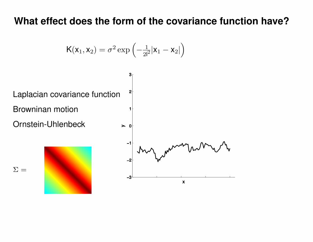
What effect does the form of the covariance function have?
−3
−2
−1
0
1
2
3
x
y
−3
−2
−1
0
1
2
3
x
y
−3
−2
−1
0
1
2
3
x
y
−3
−2
−1
0
1
2
3
x
y
−3
−2
−1
0
1
2
3
x
y
−3
−2
−1
0
1
2
3
x
y
−3
−2
−1
0
1
2
3
x
y
−3
−2
−1
0
1
2
3
x
y
−3
−2
−1
0
1
2
3
x
y
−3
−2
−1
0
1
2
3
x
y
Σ =
Laplacian covariance function
Browninan motion
Ornstein-Uhlenbeck
K(x1, x2) = σ2 exp(− 1
2l2|x1 − x2|
)

What effect does the form of the covariance function have?
−3
−2
−1
0
1
2
3
x
y
Σ =
Laplacian covariance function
Browninan motion
Ornstein-Uhlenbeck
K(x1, x2) = σ2 exp(− 1
2l2|x1 − x2|
)
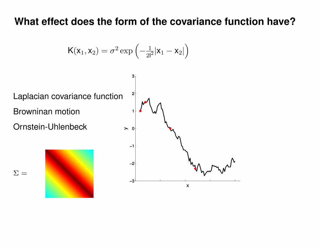
What effect does the form of the covariance function have?
−3
−2
−1
0
1
2
3
x
y
−3
−2
−1
0
1
2
3
x
y
Σ =
Laplacian covariance function
Browninan motion
Ornstein-Uhlenbeck
K(x1, x2) = σ2 exp(− 1
2l2|x1 − x2|
)
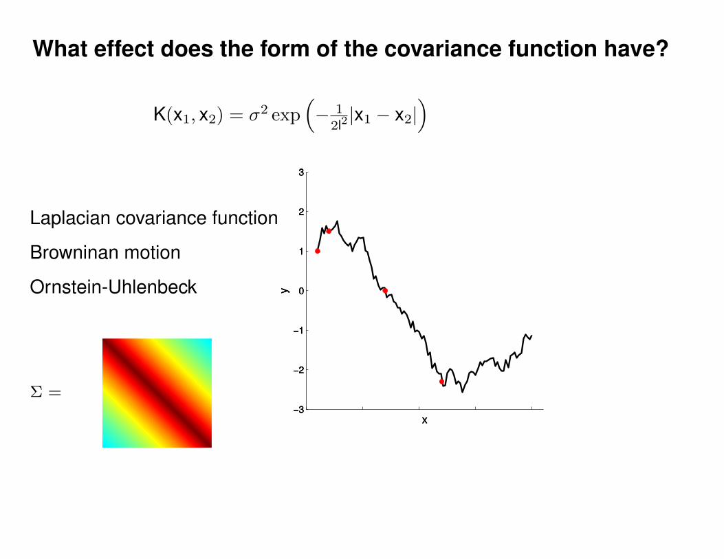
What effect does the form of the covariance function have?
−3
−2
−1
0
1
2
3
x
y
−3
−2
−1
0
1
2
3
x
y
−3
−2
−1
0
1
2
3
x
y
Σ =
Laplacian covariance function
Browninan motion
Ornstein-Uhlenbeck
K(x1, x2) = σ2 exp(− 1
2l2|x1 − x2|
)

What effect does the form of the covariance function have?
−3
−2
−1
0
1
2
3
x
y
−3
−2
−1
0
1
2
3
x
y
−3
−2
−1
0
1
2
3
x
y
−3
−2
−1
0
1
2
3
x
y
Σ =
Laplacian covariance function
Browninan motion
Ornstein-Uhlenbeck
K(x1, x2) = σ2 exp(− 1
2l2|x1 − x2|
)

What effect does the form of the covariance function have?
−3
−2
−1
0
1
2
3
x
y
−3
−2
−1
0
1
2
3
x
y
−3
−2
−1
0
1
2
3
x
y
−3
−2
−1
0
1
2
3
x
y
−3
−2
−1
0
1
2
3
x
y
Σ =
Laplacian covariance function
Browninan motion
Ornstein-Uhlenbeck
K(x1, x2) = σ2 exp(− 1
2l2|x1 − x2|
)

What effect does the form of the covariance function have?
−3
−2
−1
0
1
2
3
x
y
−3
−2
−1
0
1
2
3
x
y
−3
−2
−1
0
1
2
3
x
y
−3
−2
−1
0
1
2
3
x
y
−3
−2
−1
0
1
2
3
x
y
−3
−2
−1
0
1
2
3
x
y
Σ =
Laplacian covariance function
Browninan motion
Ornstein-Uhlenbeck
K(x1, x2) = σ2 exp(− 1
2l2|x1 − x2|
)
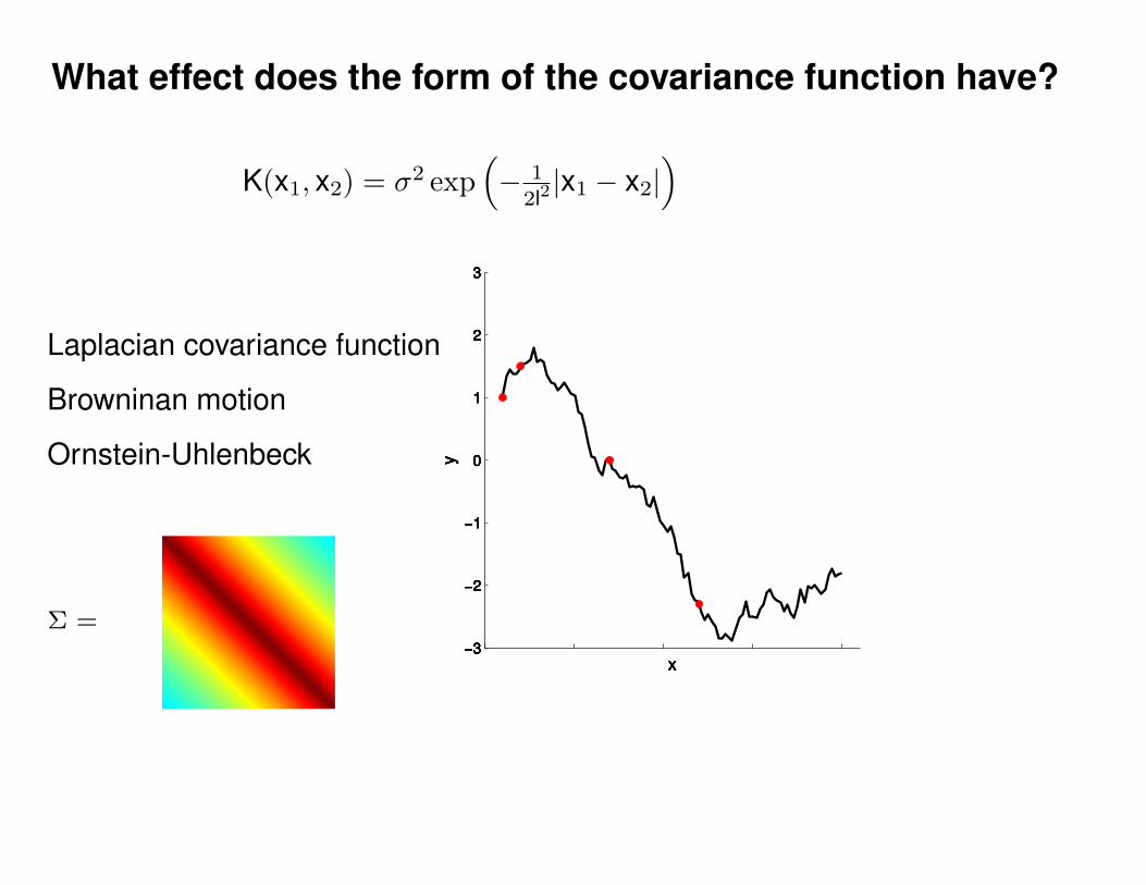
What effect does the form of the covariance function have?
−3
−2
−1
0
1
2
3
x
y
−3
−2
−1
0
1
2
3
x
y
−3
−2
−1
0
1
2
3
x
y
−3
−2
−1
0
1
2
3
x
y
−3
−2
−1
0
1
2
3
x
y
−3
−2
−1
0
1
2
3
x
y
−3
−2
−1
0
1
2
3
x
y
−3
−2
−1
0
1
2
3
x
y
−3
−2
−1
0
1
2
3
x
y
−3
−2
−1
0
1
2
3
x
y
Σ =
Laplacian covariance function
Browninan motion
Ornstein-Uhlenbeck
K(x1, x2) = σ2 exp(− 1
2l2|x1 − x2|
)
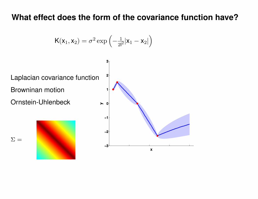
What effect does the form of the covariance function have?
−3
−2
−1
0
1
2
3
x
y
−3
−2
−1
0
1
2
3
x
y
−3
−2
−1
0
1
2
3
x
y
−3
−2
−1
0
1
2
3
x
y
−3
−2
−1
0
1
2
3
x
y
−3
−2
−1
0
1
2
3
x
y
−3
−2
−1
0
1
2
3
x
y
−3
−2
−1
0
1
2
3
x
y
−3
−2
−1
0
1
2
3
x
y
−3
−2
−1
0
1
2
3
x
y
Σ =
Laplacian covariance function
Browninan motion
Ornstein-Uhlenbeck
K(x1, x2) = σ2 exp(− 1
2l2|x1 − x2|
)

What effect does the form of the covariance function have?
−3
−2
−1
0
1
2
3
x
y
Σ =
Rational Quadratic
K(x1, x2) = σ2(
1 + 1
2αl2|x1 − x2|
)−α

What effect does the form of the covariance function have?
−3
−2
−1
0
1
2
3
x
y
−3
−2
−1
0
1
2
3
x
y
Σ =
K(x1, x2) = σ2(
1 + 1
2αl2|x1 − x2|
)−α
Rational Quadratic

What effect does the form of the covariance function have?
−3
−2
−1
0
1
2
3
x
y
−3
−2
−1
0
1
2
3
x
y
−3
−2
−1
0
1
2
3
x
y
Σ =
K(x1, x2) = σ2(
1 + 1
2αl2|x1 − x2|
)−α
Rational Quadratic

What effect does the form of the covariance function have?
−3
−2
−1
0
1
2
3
x
y
−3
−2
−1
0
1
2
3
x
y
−3
−2
−1
0
1
2
3
x
y
−3
−2
−1
0
1
2
3
x
y
Σ =
K(x1, x2) = σ2(
1 + 1
2αl2|x1 − x2|
)−α
Rational Quadratic

What effect does the form of the covariance function have?
−3
−2
−1
0
1
2
3
x
y
−3
−2
−1
0
1
2
3
x
y
−3
−2
−1
0
1
2
3
x
y
−3
−2
−1
0
1
2
3
x
y
−3
−2
−1
0
1
2
3
x
y
Σ =
K(x1, x2) = σ2(
1 + 1
2αl2|x1 − x2|
)−α
Rational Quadratic
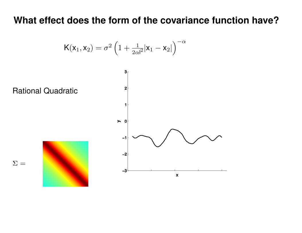
What effect does the form of the covariance function have?
−3
−2
−1
0
1
2
3
x
y
−3
−2
−1
0
1
2
3
x
y
−3
−2
−1
0
1
2
3
x
y
−3
−2
−1
0
1
2
3
x
y
−3
−2
−1
0
1
2
3
x
y
−3
−2
−1
0
1
2
3
x
y
Σ =
K(x1, x2) = σ2(
1 + 1
2αl2|x1 − x2|
)−α
Rational Quadratic

What effect does the form of the covariance function have?
−3
−2
−1
0
1
2
3
x
y
−3
−2
−1
0
1
2
3
x
y
−3
−2
−1
0
1
2
3
x
y
−3
−2
−1
0
1
2
3
x
y
−3
−2
−1
0
1
2
3
x
y
−3
−2
−1
0
1
2
3
x
y
−3
−2
−1
0
1
2
3
x
y
Σ =
K(x1, x2) = σ2(
1 + 1
2αl2|x1 − x2|
)−α
Rational Quadratic

What effect does the form of the covariance function have?
−3
−2
−1
0
1
2
3
x
y
−3
−2
−1
0
1
2
3
x
y
−3
−2
−1
0
1
2
3
x
y
−3
−2
−1
0
1
2
3
x
y
−3
−2
−1
0
1
2
3
x
y
−3
−2
−1
0
1
2
3
x
y
−3
−2
−1
0
1
2
3
x
y
−3
−2
−1
0
1
2
3
x
y
Σ =
K(x1, x2) = σ2(
1 + 1
2αl2|x1 − x2|
)−α
Rational Quadratic
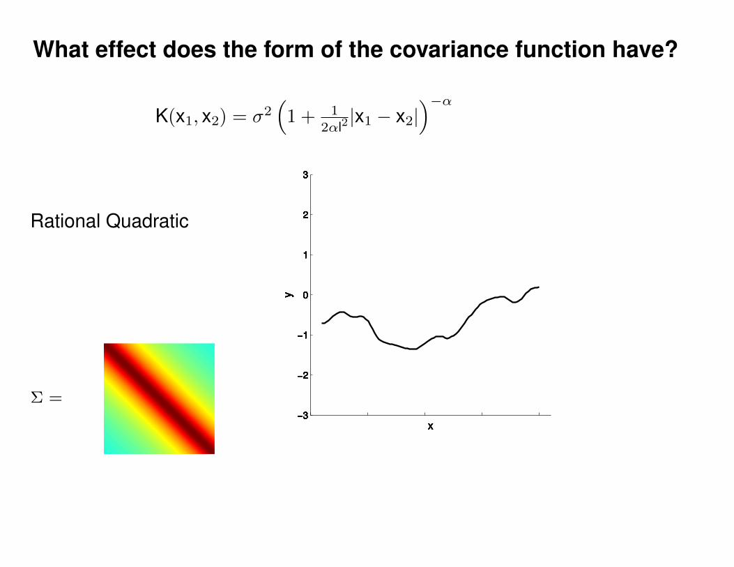
What effect does the form of the covariance function have?
−3
−2
−1
0
1
2
3
x
y
−3
−2
−1
0
1
2
3
x
y
−3
−2
−1
0
1
2
3
x
y
−3
−2
−1
0
1
2
3
x
y
−3
−2
−1
0
1
2
3
x
y
−3
−2
−1
0
1
2
3
x
y
−3
−2
−1
0
1
2
3
x
y
−3
−2
−1
0
1
2
3
x
y
−3
−2
−1
0
1
2
3
x
y
−3
−2
−1
0
1
2
3
x
y
Σ =
K(x1, x2) = σ2(
1 + 1
2αl2|x1 − x2|
)−α
Rational Quadratic

What effect does the form of the covariance function have?
−3
−2
−1
0
1
2
3
x
y
Σ =
K(x1, x2) = σ2(
1 + 1
2αl2|x1 − x2|
)−α
Rational Quadratic

What effect does the form of the covariance function have?
−3
−2
−1
0
1
2
3
x
y
−3
−2
−1
0
1
2
3
x
y
Σ =
K(x1, x2) = σ2(
1 + 1
2αl2|x1 − x2|
)−α
Rational Quadratic

What effect does the form of the covariance function have?
−3
−2
−1
0
1
2
3
x
y
−3
−2
−1
0
1
2
3
x
y
−3
−2
−1
0
1
2
3
x
y
Σ =
K(x1, x2) = σ2(
1 + 1
2αl2|x1 − x2|
)−α
Rational Quadratic

What effect does the form of the covariance function have?
−3
−2
−1
0
1
2
3
x
y
−3
−2
−1
0
1
2
3
x
y
−3
−2
−1
0
1
2
3
x
y
−3
−2
−1
0
1
2
3
x
y
Σ =
K(x1, x2) = σ2(
1 + 1
2αl2|x1 − x2|
)−α
Rational Quadratic

What effect does the form of the covariance function have?
−3
−2
−1
0
1
2
3
x
y
−3
−2
−1
0
1
2
3
x
y
−3
−2
−1
0
1
2
3
x
y
−3
−2
−1
0
1
2
3
x
y
−3
−2
−1
0
1
2
3
x
y
Σ =
K(x1, x2) = σ2(
1 + 1
2αl2|x1 − x2|
)−α
Rational Quadratic

What effect does the form of the covariance function have?
−3
−2
−1
0
1
2
3
x
y
−3
−2
−1
0
1
2
3
x
y
−3
−2
−1
0
1
2
3
x
y
−3
−2
−1
0
1
2
3
x
y
−3
−2
−1
0
1
2
3
x
y
−3
−2
−1
0
1
2
3
x
y
Σ =
K(x1, x2) = σ2(
1 + 1
2αl2|x1 − x2|
)−α
Rational Quadratic

What effect does the form of the covariance function have?
−3
−2
−1
0
1
2
3
x
y
−3
−2
−1
0
1
2
3
x
y
−3
−2
−1
0
1
2
3
x
y
−3
−2
−1
0
1
2
3
x
y
−3
−2
−1
0
1
2
3
x
y
−3
−2
−1
0
1
2
3
x
y
−3
−2
−1
0
1
2
3
x
y
Σ =
K(x1, x2) = σ2(
1 + 1
2αl2|x1 − x2|
)−α
Rational Quadratic

What effect does the form of the covariance function have?
−3
−2
−1
0
1
2
3
x
y
−3
−2
−1
0
1
2
3
x
y
−3
−2
−1
0
1
2
3
x
y
−3
−2
−1
0
1
2
3
x
y
−3
−2
−1
0
1
2
3
x
y
−3
−2
−1
0
1
2
3
x
y
−3
−2
−1
0
1
2
3
x
y
−3
−2
−1
0
1
2
3
x
y
Σ =
Rational Quadratic
K(x1, x2) = σ2(
1 + 1
2αl2|x1 − x2|
)−α

What effect does the form of the covariance function have?
−3
−2
−1
0
1
2
3
x
y
−3
−2
−1
0
1
2
3
x
y
−3
−2
−1
0
1
2
3
x
y
−3
−2
−1
0
1
2
3
x
y
−3
−2
−1
0
1
2
3
x
y
−3
−2
−1
0
1
2
3
x
y
−3
−2
−1
0
1
2
3
x
y
−3
−2
−1
0
1
2
3
x
y
−3
−2
−1
0
1
2
3
x
y
−3
−2
−1
0
1
2
3
x
y
Σ =
Rational Quadratic
K(x1, x2) = σ2(
1 + 1
2αl2|x1 − x2|
)−α
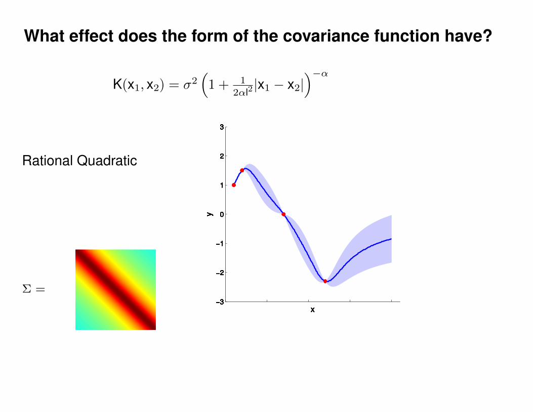
What effect does the form of the covariance function have?
−3
−2
−1
0
1
2
3
x
y
−3
−2
−1
0
1
2
3
x
y
−3
−2
−1
0
1
2
3
x
y
−3
−2
−1
0
1
2
3
x
y
−3
−2
−1
0
1
2
3
x
y
−3
−2
−1
0
1
2
3
x
y
−3
−2
−1
0
1
2
3
x
y
−3
−2
−1
0
1
2
3
x
y
−3
−2
−1
0
1
2
3
x
y
−3
−2
−1
0
1
2
3
x
y
Σ =
Rational Quadratic
K(x1, x2) = σ2(
1 + 1
2αl2|x1 − x2|
)−α

What effect does the form of the covariance function have?
−3
−2
−1
0
1
2
3
x
y
Σ =
Periodic
sinusoid × squared exponential
K(x1, x2) = σ2 cos(ω(x1 − x2)) exp(− 1
2l2(x1 − x2)2
)
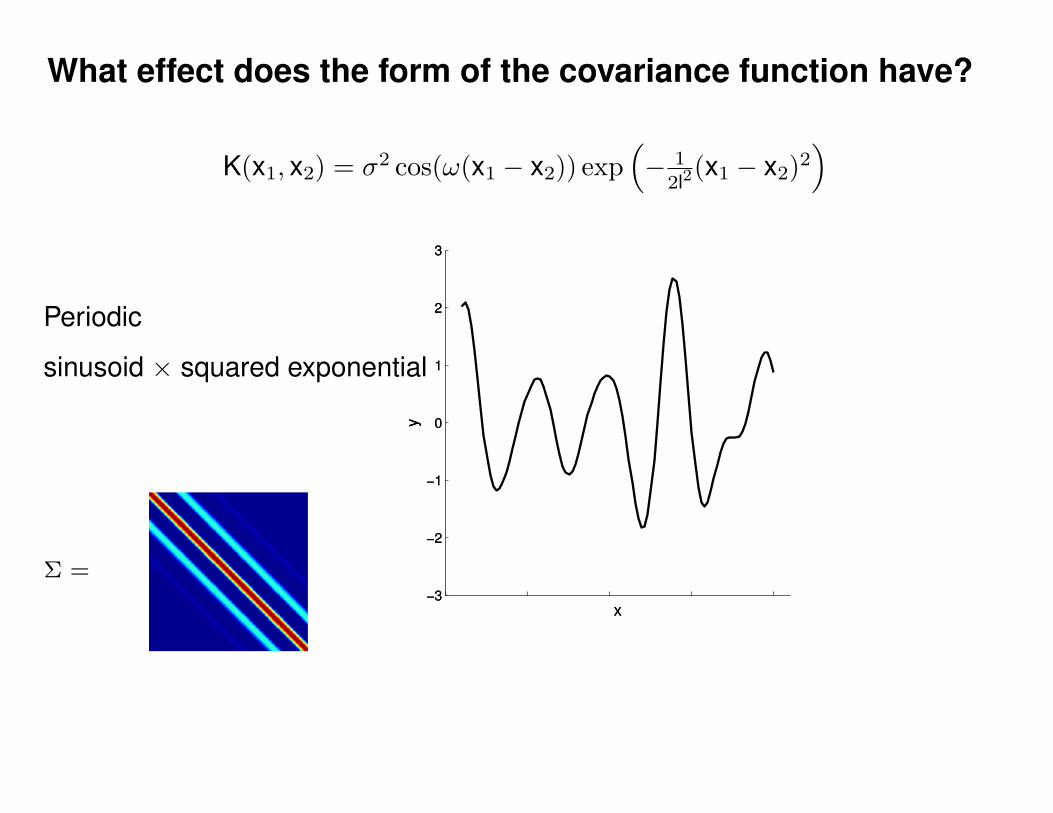
What effect does the form of the covariance function have?
−3
−2
−1
0
1
2
3
x
y
−3
−2
−1
0
1
2
3
x
y
Σ =
K(x1, x2) = σ2 cos(ω(x1 − x2)) exp(− 1
2l2(x1 − x2)2
)
Periodic
sinusoid × squared exponential

What effect does the form of the covariance function have?
−3
−2
−1
0
1
2
3
x
y
−3
−2
−1
0
1
2
3
x
y
−3
−2
−1
0
1
2
3
x
y
Σ =
K(x1, x2) = σ2 cos(ω(x1 − x2)) exp(− 1
2l2(x1 − x2)2
)
Periodic
sinusoid × squared exponential
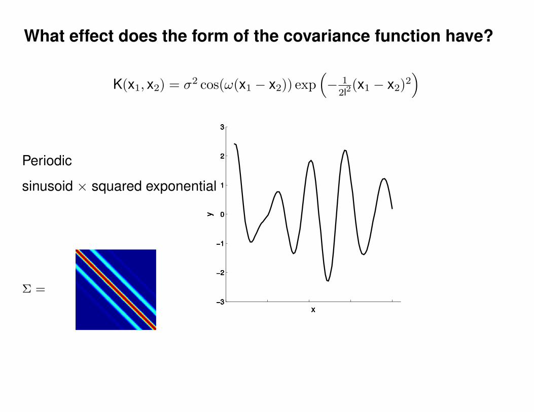
What effect does the form of the covariance function have?
−3
−2
−1
0
1
2
3
x
y
−3
−2
−1
0
1
2
3
x
y
−3
−2
−1
0
1
2
3
x
y
−3
−2
−1
0
1
2
3
x
y
Σ =
K(x1, x2) = σ2 cos(ω(x1 − x2)) exp(− 1
2l2(x1 − x2)2
)
Periodic
sinusoid × squared exponential
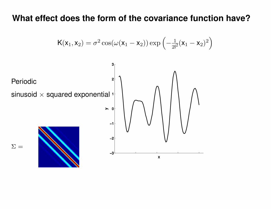
What effect does the form of the covariance function have?
−3
−2
−1
0
1
2
3
x
y
−3
−2
−1
0
1
2
3
x
y
−3
−2
−1
0
1
2
3
x
y
−3
−2
−1
0
1
2
3
x
y
−3
−2
−1
0
1
2
3
x
y
Σ =
K(x1, x2) = σ2 cos(ω(x1 − x2)) exp(− 1
2l2(x1 − x2)2
)
Periodic
sinusoid × squared exponential
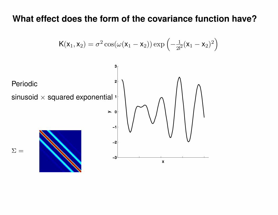
What effect does the form of the covariance function have?
−3
−2
−1
0
1
2
3
x
y
−3
−2
−1
0
1
2
3
x
y
−3
−2
−1
0
1
2
3
x
y
−3
−2
−1
0
1
2
3
x
y
−3
−2
−1
0
1
2
3
x
y
−3
−2
−1
0
1
2
3
x
y
Σ =
K(x1, x2) = σ2 cos(ω(x1 − x2)) exp(− 1
2l2(x1 − x2)2
)
Periodic
sinusoid × squared exponential

What effect does the form of the covariance function have?
−3
−2
−1
0
1
2
3
x
y
−3
−2
−1
0
1
2
3
x
y
−3
−2
−1
0
1
2
3
x
y
−3
−2
−1
0
1
2
3
x
y
−3
−2
−1
0
1
2
3
x
y
−3
−2
−1
0
1
2
3
x
y
−3
−2
−1
0
1
2
3
x
y
−3
−2
−1
0
1
2
3
x
y
Σ =
K(x1, x2) = σ2 cos(ω(x1 − x2)) exp(− 1
2l2(x1 − x2)2
)
Periodic
sinusoid × squared exponential
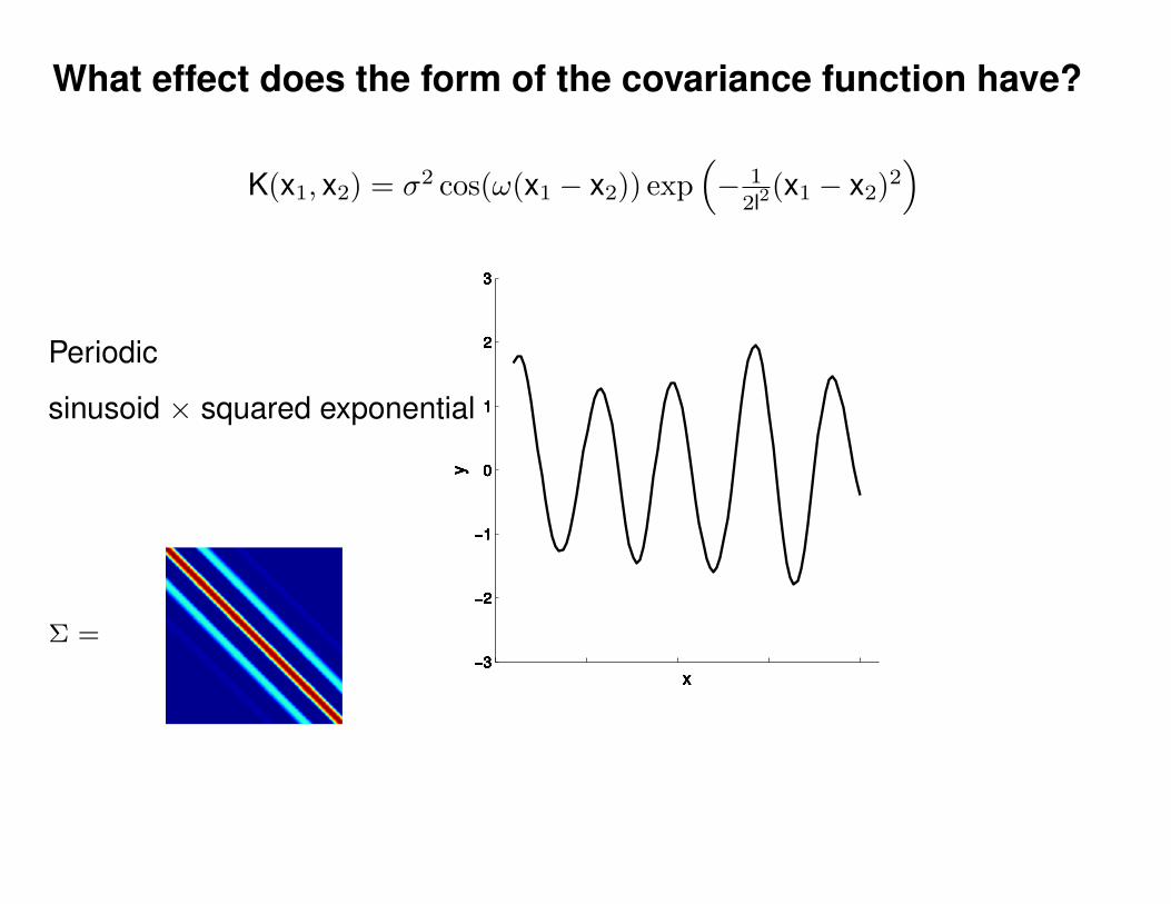
What effect does the form of the covariance function have?
−3
−2
−1
0
1
2
3
x
y
−3
−2
−1
0
1
2
3
x
y
−3
−2
−1
0
1
2
3
x
y
−3
−2
−1
0
1
2
3
x
y
−3
−2
−1
0
1
2
3
x
y
−3
−2
−1
0
1
2
3
x
y
−3
−2
−1
0
1
2
3
x
y
−3
−2
−1
0
1
2
3
x
y
−3
−2
−1
0
1
2
3
x
y
Σ =
K(x1, x2) = σ2 cos(ω(x1 − x2)) exp(− 1
2l2(x1 − x2)2
)
Periodic
sinusoid × squared exponential
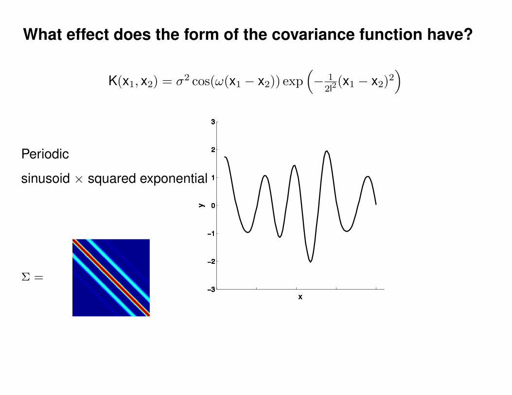
What effect does the form of the covariance function have?
−3
−2
−1
0
1
2
3
x
y
−3
−2
−1
0
1
2
3
x
y
−3
−2
−1
0
1
2
3
x
y
−3
−2
−1
0
1
2
3
x
y
−3
−2
−1
0
1
2
3
x
y
−3
−2
−1
0
1
2
3
x
y
−3
−2
−1
0
1
2
3
x
y
−3
−2
−1
0
1
2
3
x
y
−3
−2
−1
0
1
2
3
x
y
−3
−2
−1
0
1
2
3
x
y
Σ =
K(x1, x2) = σ2 cos(ω(x1 − x2)) exp(− 1
2l2(x1 − x2)2
)
Periodic
sinusoid × squared exponential

What effect does the form of the covariance function have?
−3
−2
−1
0
1
2
3
x
y
Σ =
K(x1, x2) = σ2 cos(ω(x1 − x2)) exp(− 1
2l2(x1 − x2)2
)
Periodic
sinusoid × squared exponential

What effect does the form of the covariance function have?
−3
−2
−1
0
1
2
3
x
y
−3
−2
−1
0
1
2
3
x
y
Σ =
K(x1, x2) = σ2 cos(ω(x1 − x2)) exp(− 1
2l2(x1 − x2)2
)
Periodic
sinusoid × squared exponential
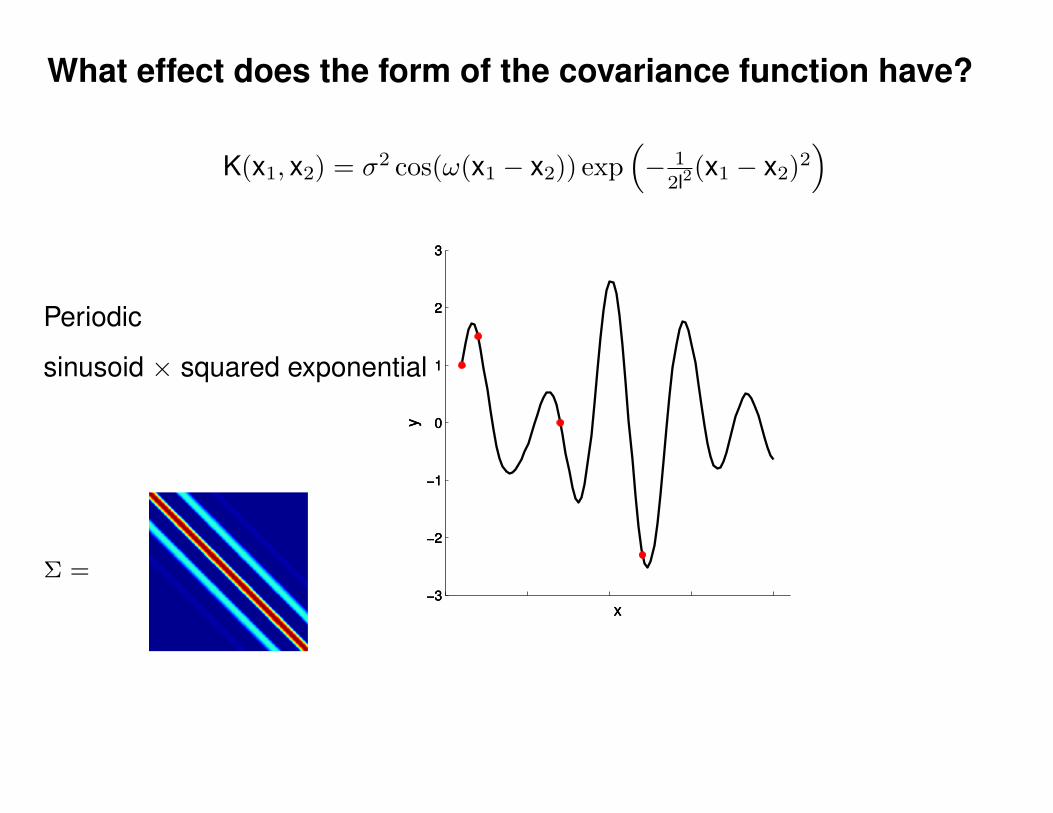
What effect does the form of the covariance function have?
−3
−2
−1
0
1
2
3
x
y
−3
−2
−1
0
1
2
3
x
y
−3
−2
−1
0
1
2
3
x
y
Σ =
K(x1, x2) = σ2 cos(ω(x1 − x2)) exp(− 1
2l2(x1 − x2)2
)
Periodic
sinusoid × squared exponential

What effect does the form of the covariance function have?
−3
−2
−1
0
1
2
3
x
y
−3
−2
−1
0
1
2
3
x
y
−3
−2
−1
0
1
2
3
x
y
−3
−2
−1
0
1
2
3
x
y
Σ =
K(x1, x2) = σ2 cos(ω(x1 − x2)) exp(− 1
2l2(x1 − x2)2
)
Periodic
sinusoid × squared exponential

What effect does the form of the covariance function have?
−3
−2
−1
0
1
2
3
x
y
−3
−2
−1
0
1
2
3
x
y
−3
−2
−1
0
1
2
3
x
y
−3
−2
−1
0
1
2
3
x
y
−3
−2
−1
0
1
2
3
x
y
Σ =
K(x1, x2) = σ2 cos(ω(x1 − x2)) exp(− 1
2l2(x1 − x2)2
)
Periodic
sinusoid × squared exponential
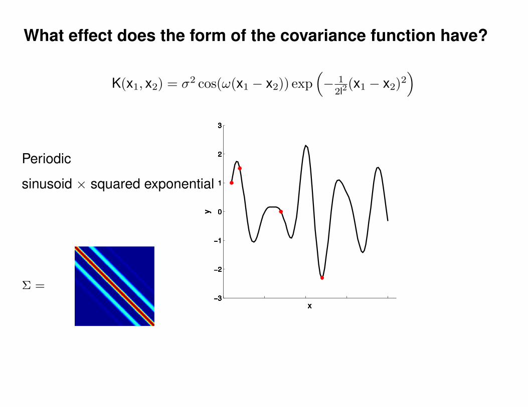
What effect does the form of the covariance function have?
−3
−2
−1
0
1
2
3
x
y
−3
−2
−1
0
1
2
3
x
y
−3
−2
−1
0
1
2
3
x
y
−3
−2
−1
0
1
2
3
x
y
−3
−2
−1
0
1
2
3
x
y
−3
−2
−1
0
1
2
3
x
y
Σ =
K(x1, x2) = σ2 cos(ω(x1 − x2)) exp(− 1
2l2(x1 − x2)2
)
Periodic
sinusoid × squared exponential

What effect does the form of the covariance function have?
−3
−2
−1
0
1
2
3
x
y
−3
−2
−1
0
1
2
3
x
y
−3
−2
−1
0
1
2
3
x
y
−3
−2
−1
0
1
2
3
x
y
−3
−2
−1
0
1
2
3
x
y
−3
−2
−1
0
1
2
3
x
y
−3
−2
−1
0
1
2
3
x
y
−3
−2
−1
0
1
2
3
x
y
−3
−2
−1
0
1
2
3
x
y
Σ =
K(x1, x2) = σ2 cos(ω(x1 − x2)) exp(− 1
2l2(x1 − x2)2
)
Periodic
sinusoid × squared exponential
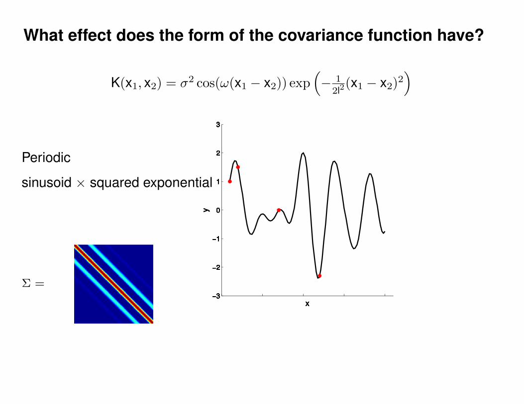
What effect does the form of the covariance function have?
−3
−2
−1
0
1
2
3
x
y
−3
−2
−1
0
1
2
3
x
y
−3
−2
−1
0
1
2
3
x
y
−3
−2
−1
0
1
2
3
x
y
−3
−2
−1
0
1
2
3
x
y
−3
−2
−1
0
1
2
3
x
y
−3
−2
−1
0
1
2
3
x
y
−3
−2
−1
0
1
2
3
x
y
−3
−2
−1
0
1
2
3
x
y
−3
−2
−1
0
1
2
3
x
y
Σ =
K(x1, x2) = σ2 cos(ω(x1 − x2)) exp(− 1
2l2(x1 − x2)2
)
Periodic
sinusoid × squared exponential
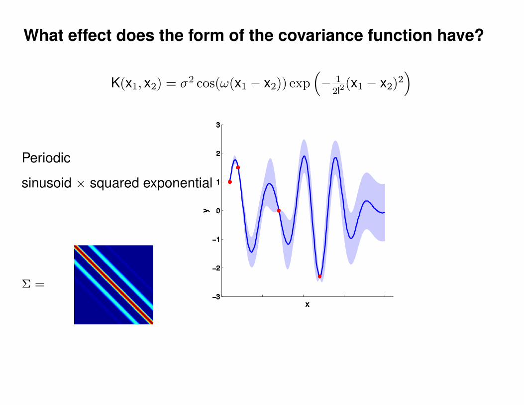
What effect does the form of the covariance function have?
−3
−2
−1
0
1
2
3
x
y
−3
−2
−1
0
1
2
3
x
y
−3
−2
−1
0
1
2
3
x
y
−3
−2
−1
0
1
2
3
x
y
−3
−2
−1
0
1
2
3
x
y
−3
−2
−1
0
1
2
3
x
y
−3
−2
−1
0
1
2
3
x
y
−3
−2
−1
0
1
2
3
x
y
−3
−2
−1
0
1
2
3
x
y
−3
−2
−1
0
1
2
3
x
y
Σ =
K(x1, x2) = σ2 cos(ω(x1 − x2)) exp(− 1
2l2(x1 − x2)2
)
Periodic
sinusoid × squared exponential
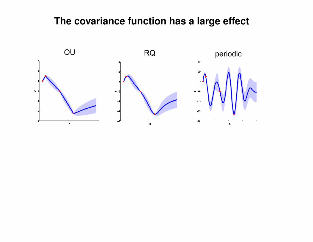
The covariance function has a large effect
−3
−2
−1
0
1
2
3
x
y
−3
−2
−1
0
1
2
3
x
y
−3
−2
−1
0
1
2
3
x
y
−3
−2
−1
0
1
2
3
x
y
−3
−2
−1
0
1
2
3
x
y
−3
−2
−1
0
1
2
3
x
y
−3
−2
−1
0
1
2
3
x
y
−3
−2
−1
0
1
2
3
x
y
−3
−2
−1
0
1
2
3
x
y
−3
−2
−1
0
1
2
3
x
y
−3
−2
−1
0
1
2
3
x
y
−3
−2
−1
0
1
2
3
x
y
−3
−2
−1
0
1
2
3
x
y
−3
−2
−1
0
1
2
3
x
y
−3
−2
−1
0
1
2
3
x
y
−3
−2
−1
0
1
2
3
x
y
−3
−2
−1
0
1
2
3
x
y
−3
−2
−1
0
1
2
3
x
y
−3
−2
−1
0
1
2
3
x
y
−3
−2
−1
0
1
2
3
x
y
−3
−2
−1
0
1
2
3
x
y
−3
−2
−1
0
1
2
3
x
y
−3
−2
−1
0
1
2
3
x
y
−3
−2
−1
0
1
2
3
x
y
−3
−2
−1
0
1
2
3
x
y
−3
−2
−1
0
1
2
3
x
y
−3
−2
−1
0
1
2
3
x
y
−3
−2
−1
0
1
2
3
x
y
−3
−2
−1
0
1
2
3
x
y
−3
−2
−1
0
1
2
3
x
y
OU RQ periodic
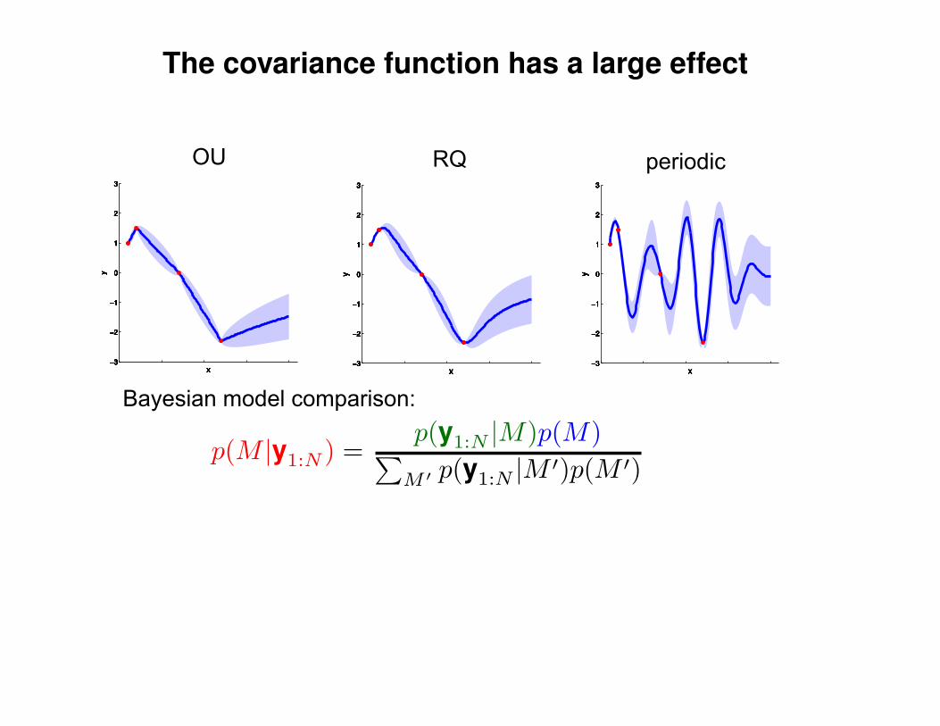
Bayesian model comparison:
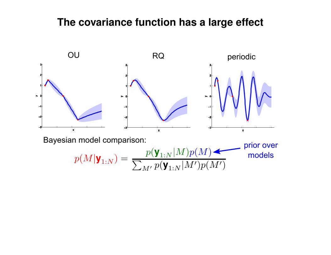
The covariance function has a large effect
−3
−2
−1
0
1
2
3
x
y
−3
−2
−1
0
1
2
3
x
y
−3
−2
−1
0
1
2
3
x
y
−3
−2
−1
0
1
2
3
x
y
−3
−2
−1
0
1
2
3
x
y
−3
−2
−1
0
1
2
3
x
y
−3
−2
−1
0
1
2
3
x
y
−3
−2
−1
0
1
2
3
x
y
−3
−2
−1
0
1
2
3
x
y
−3
−2
−1
0
1
2
3
x
y
−3
−2
−1
0
1
2
3
x
y
−3
−2
−1
0
1
2
3
x
y
−3
−2
−1
0
1
2
3
x
y
−3
−2
−1
0
1
2
3
x
y
−3
−2
−1
0
1
2
3
x
y
−3
−2
−1
0
1
2
3
x
y
−3
−2
−1
0
1
2
3
x
y
−3
−2
−1
0
1
2
3
x
y
−3
−2
−1
0
1
2
3
x
y
−3
−2
−1
0
1
2
3
x
y
−3
−2
−1
0
1
2
3
x
y
−3
−2
−1
0
1
2
3
x
y
−3
−2
−1
0
1
2
3
x
y
−3
−2
−1
0
1
2
3
x
y
−3
−2
−1
0
1
2
3
x
y
−3
−2
−1
0
1
2
3
x
y
−3
−2
−1
0
1
2
3
x
y
−3
−2
−1
0
1
2
3
x
y
−3
−2
−1
0
1
2
3
x
y
−3
−2
−1
0
1
2
3
x
y
OU RQ periodic
Bayesian model comparison:prior over models
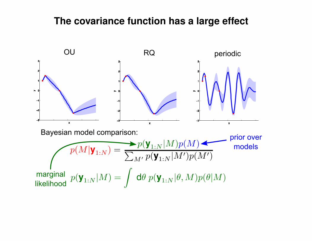
marginal likelihood
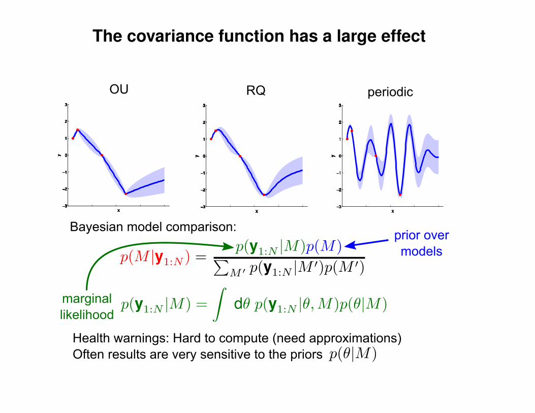
The covariance function has a large effect
Health warnings: Hard to compute (need approximations)Often results are very sensitive to the priors
−3
−2
−1
0
1
2
3
x
y
−3
−2
−1
0
1
2
3
x
y
−3
−2
−1
0
1
2
3
x
y
−3
−2
−1
0
1
2
3
x
y
−3
−2
−1
0
1
2
3
x
y
−3
−2
−1
0
1
2
3
x
y
−3
−2
−1
0
1
2
3
x
y
−3
−2
−1
0
1
2
3
x
y
−3
−2
−1
0
1
2
3
x
y
−3
−2
−1
0
1
2
3
x
y
−3
−2
−1
0
1
2
3
x
y
−3
−2
−1
0
1
2
3
x
y
−3
−2
−1
0
1
2
3
x
y
−3
−2
−1
0
1
2
3
x
y
−3
−2
−1
0
1
2
3
x
y
−3
−2
−1
0
1
2
3
x
y
−3
−2
−1
0
1
2
3
x
y
−3
−2
−1
0
1
2
3
x
y
−3
−2
−1
0
1
2
3
x
y
−3
−2
−1
0
1
2
3
x
y
−3
−2
−1
0
1
2
3
x
y
−3
−2
−1
0
1
2
3
x
y
−3
−2
−1
0
1
2
3
x
y
−3
−2
−1
0
1
2
3
x
y
−3
−2
−1
0
1
2
3
x
y
−3
−2
−1
0
1
2
3
x
y
−3
−2
−1
0
1
2
3
x
y
−3
−2
−1
0
1
2
3
x
y
−3
−2
−1
0
1
2
3
x
y
−3
−2
−1
0
1
2
3
x
y
OU RQ periodic
Bayesian model comparison:prior over models
marginal likelihood

Basis function view of Gaussian processes
−10 −8 −6 −4 −2 0 2 4 6 8 10
−1
0
1co
eff
icie
nts
−10 −8 −6 −4 −2 0 2 4 6 8 100
0.5
1
ba
sis
fu
nctio
ns
−10 −8 −6 −4 −2 0 2 4 6 8 10
−1
0
1
x
f(x)
γ ∼ N (0, 1)
g(x) = e−1
l2(x−µ)2
f(x) = γg(x)
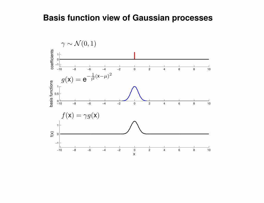
Basis function view of Gaussian processes
−10 −8 −6 −4 −2 0 2 4 6 8 10
−1
0
1co
eff
icie
nts
−10 −8 −6 −4 −2 0 2 4 6 8 100
0.5
1
ba
sis
fu
nctio
ns
−10 −8 −6 −4 −2 0 2 4 6 8 10
−1
0
1
x
f(x)
γ ∼ N (0, 1)
g(x) = e−1
l2(x−µ)2
f(x) = γg(x)

Basis function view of Gaussian processes
−10 −8 −6 −4 −2 0 2 4 6 8 10
−1
0
1co
eff
icie
nts
−10 −8 −6 −4 −2 0 2 4 6 8 100
0.5
1
ba
sis
fu
nctio
ns
−10 −8 −6 −4 −2 0 2 4 6 8 10
−1
0
1
x
f(x)
γ ∼ N (0, 1)
g(x) = e−1
l2(x−µ)2
f(x) = γg(x)

Basis function view of Gaussian processes
−10 −8 −6 −4 −2 0 2 4 6 8 10
−1
0
1co
eff
icie
nts
−10 −8 −6 −4 −2 0 2 4 6 8 100
0.5
1
ba
sis
fu
nctio
ns
−10 −8 −6 −4 −2 0 2 4 6 8 10
−1
0
1
x
f(x)
γ ∼ N (0, 1)
g(x) = e−1
l2(x−µ)2
f(x) = γg(x)

Basis function view of Gaussian processes
−10 −8 −6 −4 −2 0 2 4 6 8 10
−1
0
1co
eff
icie
nts
−10 −8 −6 −4 −2 0 2 4 6 8 100
0.5
1
ba
sis
fu
nctio
ns
−10 −8 −6 −4 −2 0 2 4 6 8 10
−1
0
1
x
f(x)
γ ∼ N (0, 1)
g(x) = e−1
l2(x−µ)2
f(x) = γg(x)

Basis function view of Gaussian processes
−10 −8 −6 −4 −2 0 2 4 6 8 10
−1
0
1co
eff
icie
nts
−10 −8 −6 −4 −2 0 2 4 6 8 100
0.5
1
ba
sis
fu
nctio
ns
−10 −8 −6 −4 −2 0 2 4 6 8 10
−1
0
1
x
f(x)
γ ∼ N (0, 1)
g(x) = e−1
l2(x−µ)2
f(x) = γg(x)
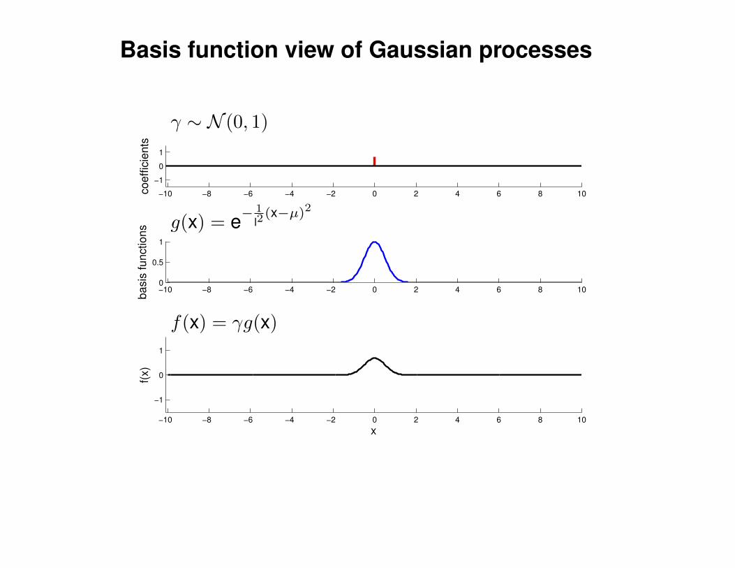
Basis function view of Gaussian processes
−10 −8 −6 −4 −2 0 2 4 6 8 10
−1
0
1co
eff
icie
nts
−10 −8 −6 −4 −2 0 2 4 6 8 100
0.5
1
ba
sis
fu
nctio
ns
−10 −8 −6 −4 −2 0 2 4 6 8 10
−1
0
1
x
f(x)
γ ∼ N (0, 1)
g(x) = e−1
l2(x−µ)2
f(x) = γg(x)
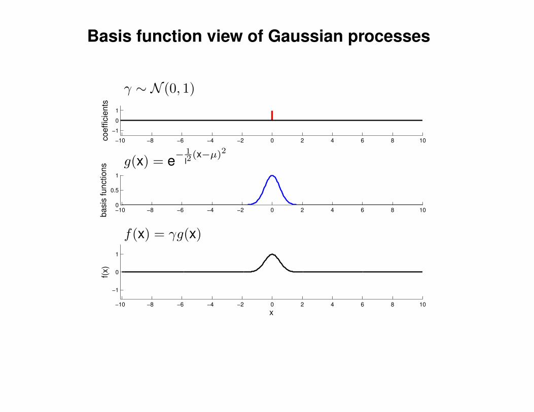
Basis function view of Gaussian processes
−10 −8 −6 −4 −2 0 2 4 6 8 10
−1
0
1co
eff
icie
nts
−10 −8 −6 −4 −2 0 2 4 6 8 100
0.5
1
ba
sis
fu
nctio
ns
−10 −8 −6 −4 −2 0 2 4 6 8 10
−1
0
1
x
f(x)
γ ∼ N (0, 1)
g(x) = e−1
l2(x−µ)2
f(x) = γg(x)

Basis function view of Gaussian processes
−10 −8 −6 −4 −2 0 2 4 6 8 10
−1
0
1co
eff
icie
nts
−10 −8 −6 −4 −2 0 2 4 6 8 100
0.5
1
ba
sis
fu
nctio
ns
−10 −8 −6 −4 −2 0 2 4 6 8 10
−1
0
1
x
f(x)
γ ∼ N (0, 1)
g(x) = e−1
l2(x−µ)2
f(x) = γg(x)
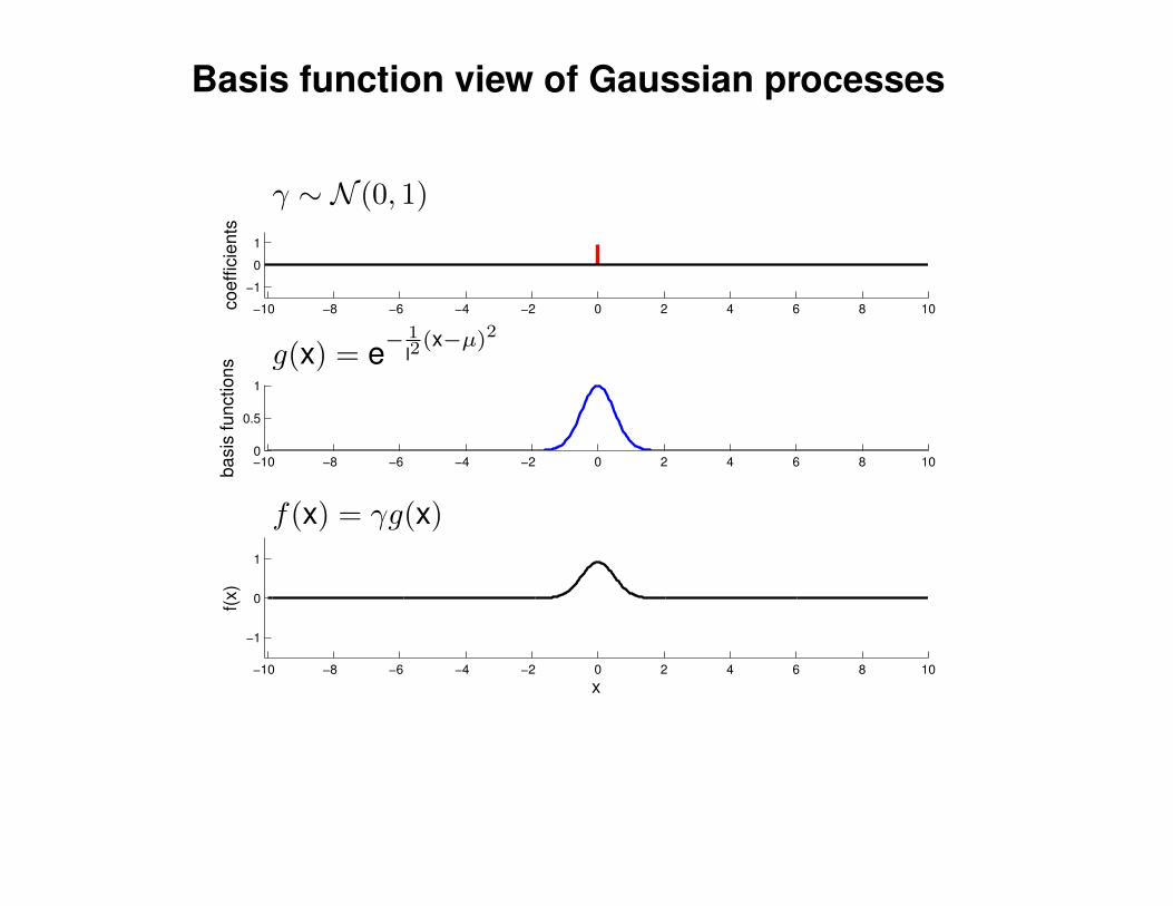
Basis function view of Gaussian processes
−10 −8 −6 −4 −2 0 2 4 6 8 10
−1
0
1co
eff
icie
nts
−10 −8 −6 −4 −2 0 2 4 6 8 100
0.5
1
ba
sis
fu
nctio
ns
−10 −8 −6 −4 −2 0 2 4 6 8 10
−1
0
1
x
f(x)
γ ∼ N (0, 1)
g(x) = e−1
l2(x−µ)2
f(x) = γg(x)
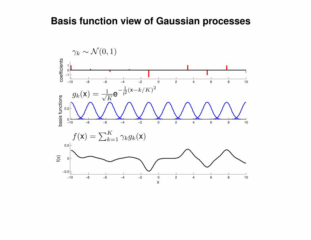
Basis function view of Gaussian processes
−10 −8 −6 −4 −2 0 2 4 6 8 10
−1
0
1
co
eff
icie
nts
−10 −8 −6 −4 −2 0 2 4 6 8 100
0.2
ba
sis
fu
nctio
ns
−10 −8 −6 −4 −2 0 2 4 6 8 10
−0.5
0
0.5
x
f(x)
γk ∼ N (0, 1)
gk(x) = 1√K
e−1
l2(x−k/K)2
f(x) =∑Kk=1 γkgk(x)

Basis function view of Gaussian processes
−10 −8 −6 −4 −2 0 2 4 6 8 10
−1
0
1
co
eff
icie
nts
−10 −8 −6 −4 −2 0 2 4 6 8 100
0.2
ba
sis
fu
nctio
ns
−10 −8 −6 −4 −2 0 2 4 6 8 10
−0.5
0
0.5
x
f(x)
γk ∼ N (0, 1)
gk(x) = 1√K
e−1
l2(x−k/K)2
f(x) =∑Kk=1 γkgk(x)
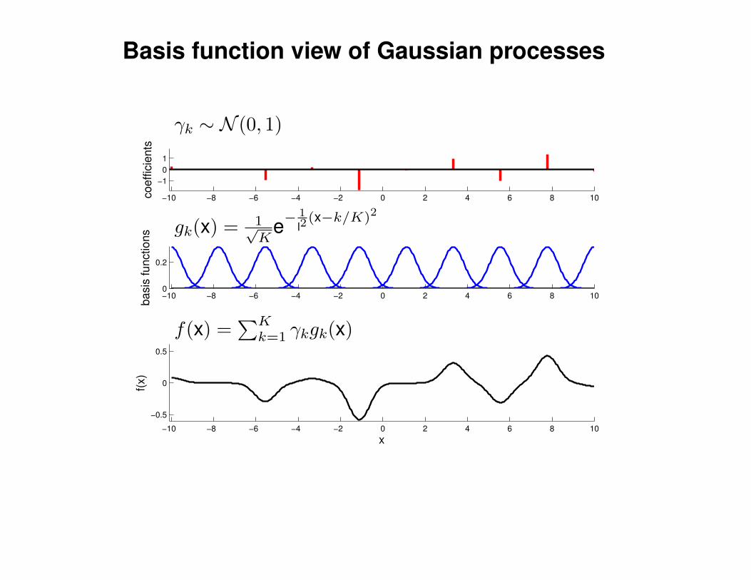
Basis function view of Gaussian processes
−10 −8 −6 −4 −2 0 2 4 6 8 10
−1
0
1
co
eff
icie
nts
−10 −8 −6 −4 −2 0 2 4 6 8 100
0.2
ba
sis
fu
nctio
ns
−10 −8 −6 −4 −2 0 2 4 6 8 10
−0.5
0
0.5
x
f(x)
γk ∼ N (0, 1)
gk(x) = 1√K
e−1
l2(x−k/K)2
f(x) =∑Kk=1 γkgk(x)
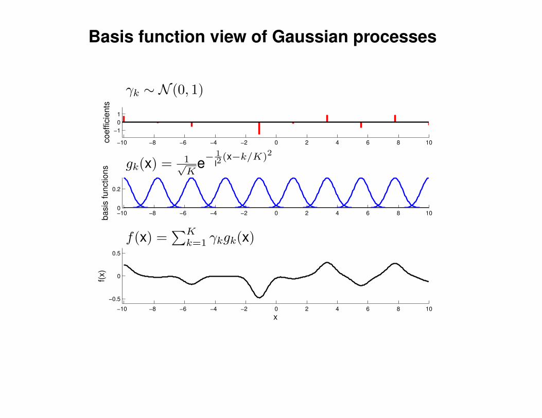
Basis function view of Gaussian processes
−10 −8 −6 −4 −2 0 2 4 6 8 10
−1
0
1
co
eff
icie
nts
−10 −8 −6 −4 −2 0 2 4 6 8 100
0.2
ba
sis
fu
nctio
ns
−10 −8 −6 −4 −2 0 2 4 6 8 10
−0.5
0
0.5
x
f(x)
γk ∼ N (0, 1)
gk(x) = 1√K
e−1
l2(x−k/K)2
f(x) =∑Kk=1 γkgk(x)
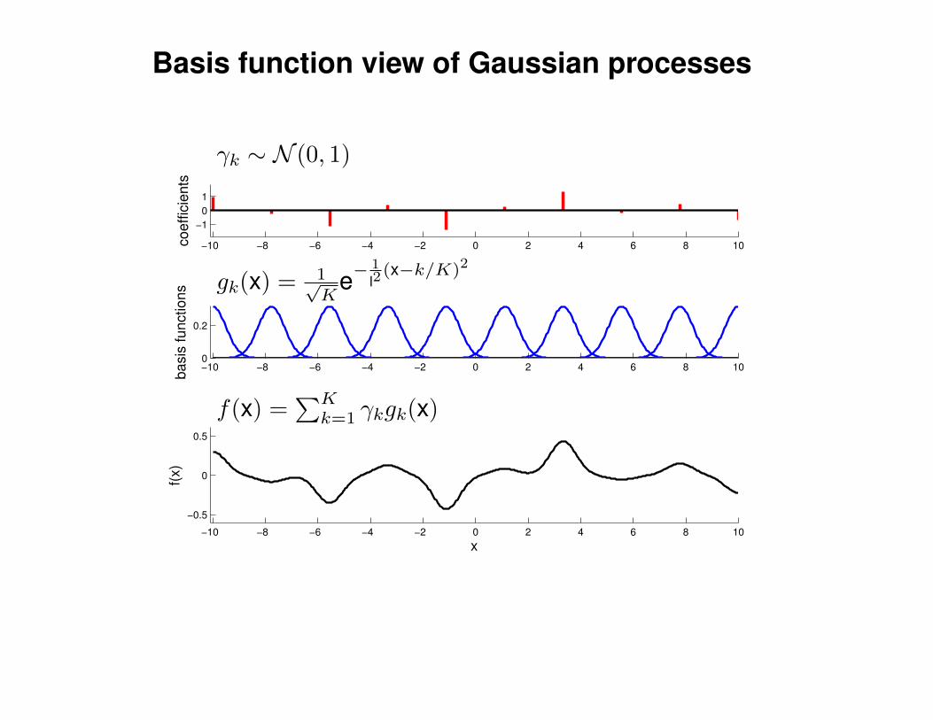
Basis function view of Gaussian processes
−10 −8 −6 −4 −2 0 2 4 6 8 10
−1
0
1
co
eff
icie
nts
−10 −8 −6 −4 −2 0 2 4 6 8 100
0.2
ba
sis
fu
nctio
ns
−10 −8 −6 −4 −2 0 2 4 6 8 10
−0.5
0
0.5
x
f(x)
γk ∼ N (0, 1)
gk(x) = 1√K
e−1
l2(x−k/K)2
f(x) =∑Kk=1 γkgk(x)
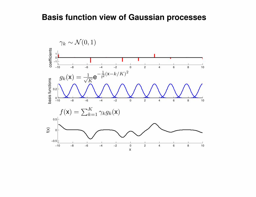
Basis function view of Gaussian processes
−10 −8 −6 −4 −2 0 2 4 6 8 10
−1
0
1
co
eff
icie
nts
−10 −8 −6 −4 −2 0 2 4 6 8 100
0.2
ba
sis
fu
nctio
ns
−10 −8 −6 −4 −2 0 2 4 6 8 10
−0.5
0
0.5
x
f(x)
γk ∼ N (0, 1)
gk(x) = 1√K
e−1
l2(x−k/K)2
f(x) =∑Kk=1 γkgk(x)
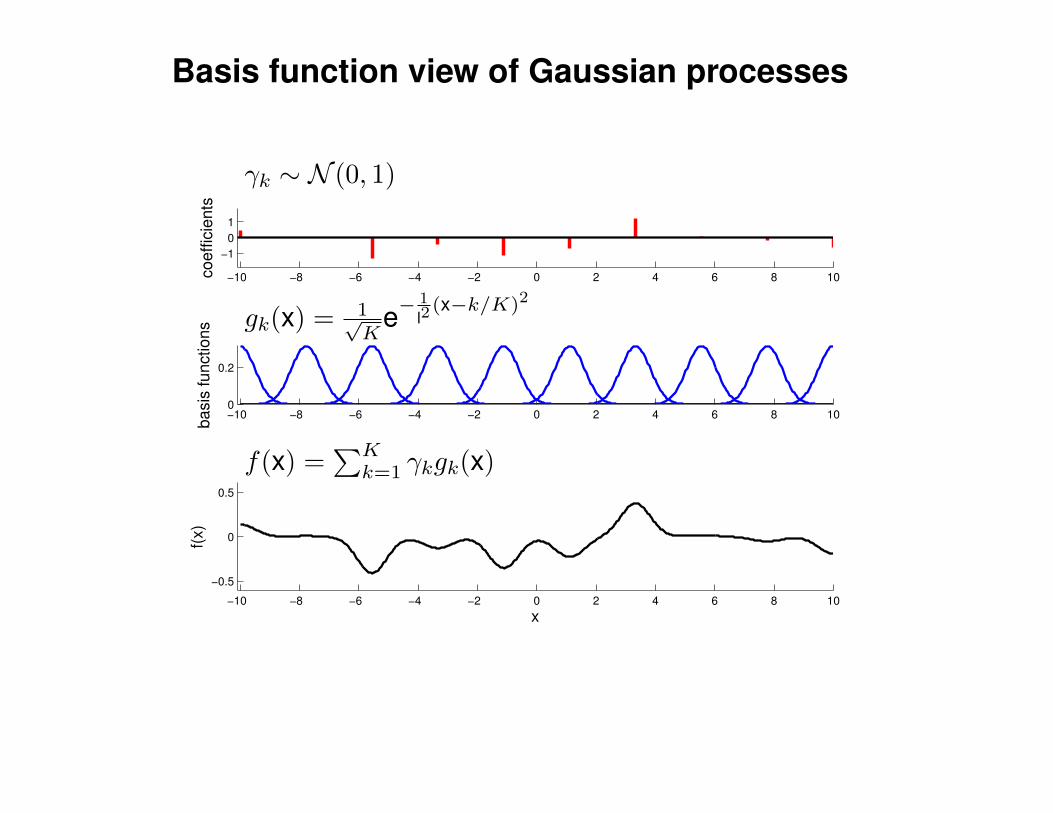
Basis function view of Gaussian processes
−10 −8 −6 −4 −2 0 2 4 6 8 10
−1
0
1
co
eff
icie
nts
−10 −8 −6 −4 −2 0 2 4 6 8 100
0.2
ba
sis
fu
nctio
ns
−10 −8 −6 −4 −2 0 2 4 6 8 10
−0.5
0
0.5
x
f(x)
γk ∼ N (0, 1)
gk(x) = 1√K
e−1
l2(x−k/K)2
f(x) =∑Kk=1 γkgk(x)
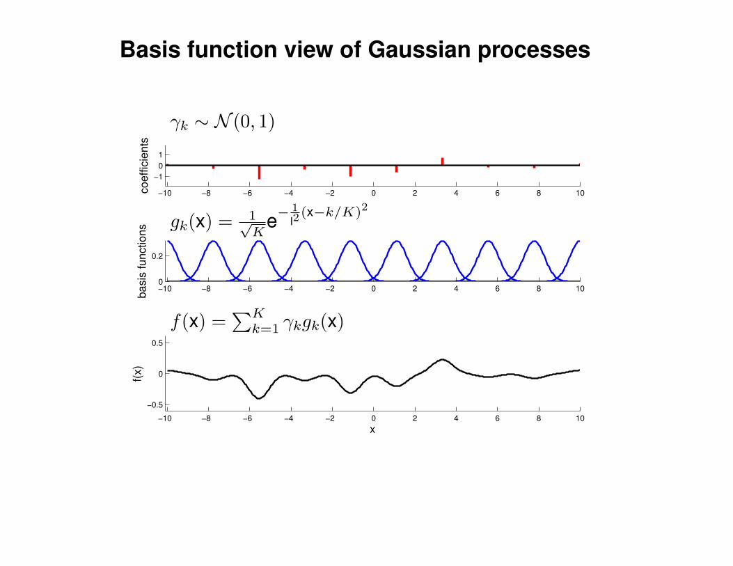
Basis function view of Gaussian processes
−10 −8 −6 −4 −2 0 2 4 6 8 10
−1
0
1
co
eff
icie
nts
−10 −8 −6 −4 −2 0 2 4 6 8 100
0.2
ba
sis
fu
nctio
ns
−10 −8 −6 −4 −2 0 2 4 6 8 10
−0.5
0
0.5
x
f(x)
γk ∼ N (0, 1)
gk(x) = 1√K
e−1
l2(x−k/K)2
f(x) =∑Kk=1 γkgk(x)
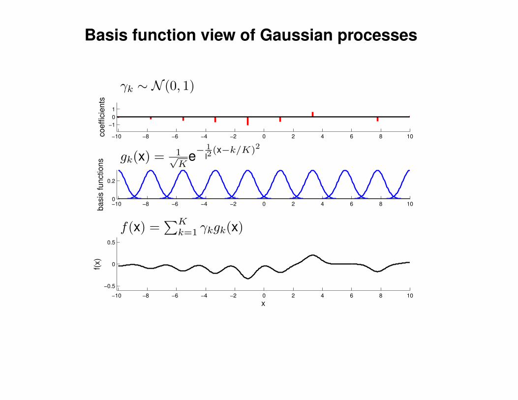
Basis function view of Gaussian processes
−10 −8 −6 −4 −2 0 2 4 6 8 10
−1
0
1
co
eff
icie
nts
−10 −8 −6 −4 −2 0 2 4 6 8 100
0.2
ba
sis
fu
nctio
ns
−10 −8 −6 −4 −2 0 2 4 6 8 10
−0.5
0
0.5
x
f(x)
γk ∼ N (0, 1)
gk(x) = 1√K
e−1
l2(x−k/K)2
f(x) =∑Kk=1 γkgk(x)
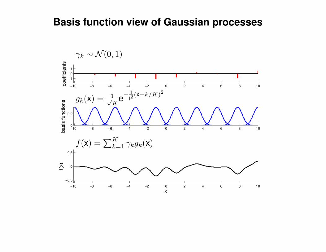
Basis function view of Gaussian processes
−10 −8 −6 −4 −2 0 2 4 6 8 10
−1
0
1
co
eff
icie
nts
−10 −8 −6 −4 −2 0 2 4 6 8 100
0.2
ba
sis
fu
nctio
ns
−10 −8 −6 −4 −2 0 2 4 6 8 10
−0.5
0
0.5
x
f(x)
γk ∼ N (0, 1)
gk(x) = 1√K
e−1
l2(x−k/K)2
f(x) =∑Kk=1 γkgk(x)
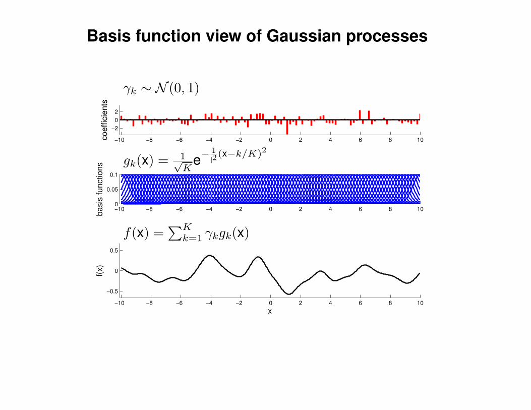
Basis function view of Gaussian processes
−10 −8 −6 −4 −2 0 2 4 6 8 10
−2
0
2
co
eff
icie
nts
−10 −8 −6 −4 −2 0 2 4 6 8 100
0.05
0.1
ba
sis
fu
nctio
ns
−10 −8 −6 −4 −2 0 2 4 6 8 10
−0.5
0
0.5
x
f(x)
γk ∼ N (0, 1)
gk(x) = 1√K
e−1
l2(x−k/K)2
f(x) =∑Kk=1 γkgk(x)
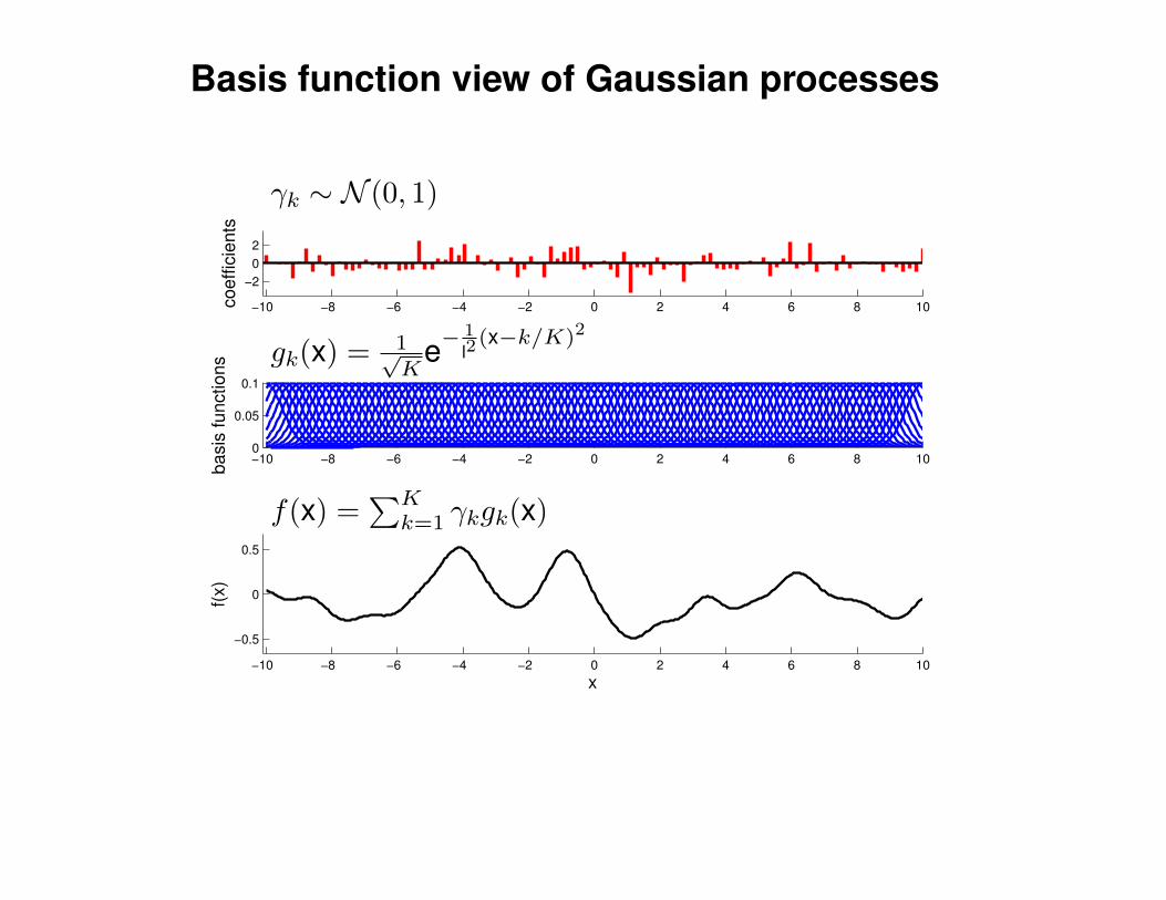
Basis function view of Gaussian processes
−10 −8 −6 −4 −2 0 2 4 6 8 10
−2
0
2
co
eff
icie
nts
−10 −8 −6 −4 −2 0 2 4 6 8 100
0.05
0.1
ba
sis
fu
nctio
ns
−10 −8 −6 −4 −2 0 2 4 6 8 10
−0.5
0
0.5
x
f(x)
γk ∼ N (0, 1)
gk(x) = 1√K
e−1
l2(x−k/K)2
f(x) =∑Kk=1 γkgk(x)
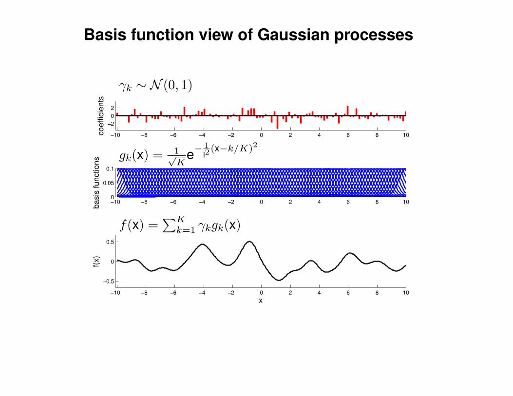
Basis function view of Gaussian processes
−10 −8 −6 −4 −2 0 2 4 6 8 10
−2
0
2
co
eff
icie
nts
−10 −8 −6 −4 −2 0 2 4 6 8 100
0.05
0.1
ba
sis
fu
nctio
ns
−10 −8 −6 −4 −2 0 2 4 6 8 10
−0.5
0
0.5
x
f(x)
γk ∼ N (0, 1)
gk(x) = 1√K
e−1
l2(x−k/K)2
f(x) =∑Kk=1 γkgk(x)

Basis function view of Gaussian processes
−10 −8 −6 −4 −2 0 2 4 6 8 10
−2
0
2
co
eff
icie
nts
−10 −8 −6 −4 −2 0 2 4 6 8 100
0.05
0.1
ba
sis
fu
nctio
ns
−10 −8 −6 −4 −2 0 2 4 6 8 10
−0.5
0
0.5
x
f(x)
γk ∼ N (0, 1)
gk(x) = 1√K
e−1
l2(x−k/K)2
f(x) =∑Kk=1 γkgk(x)
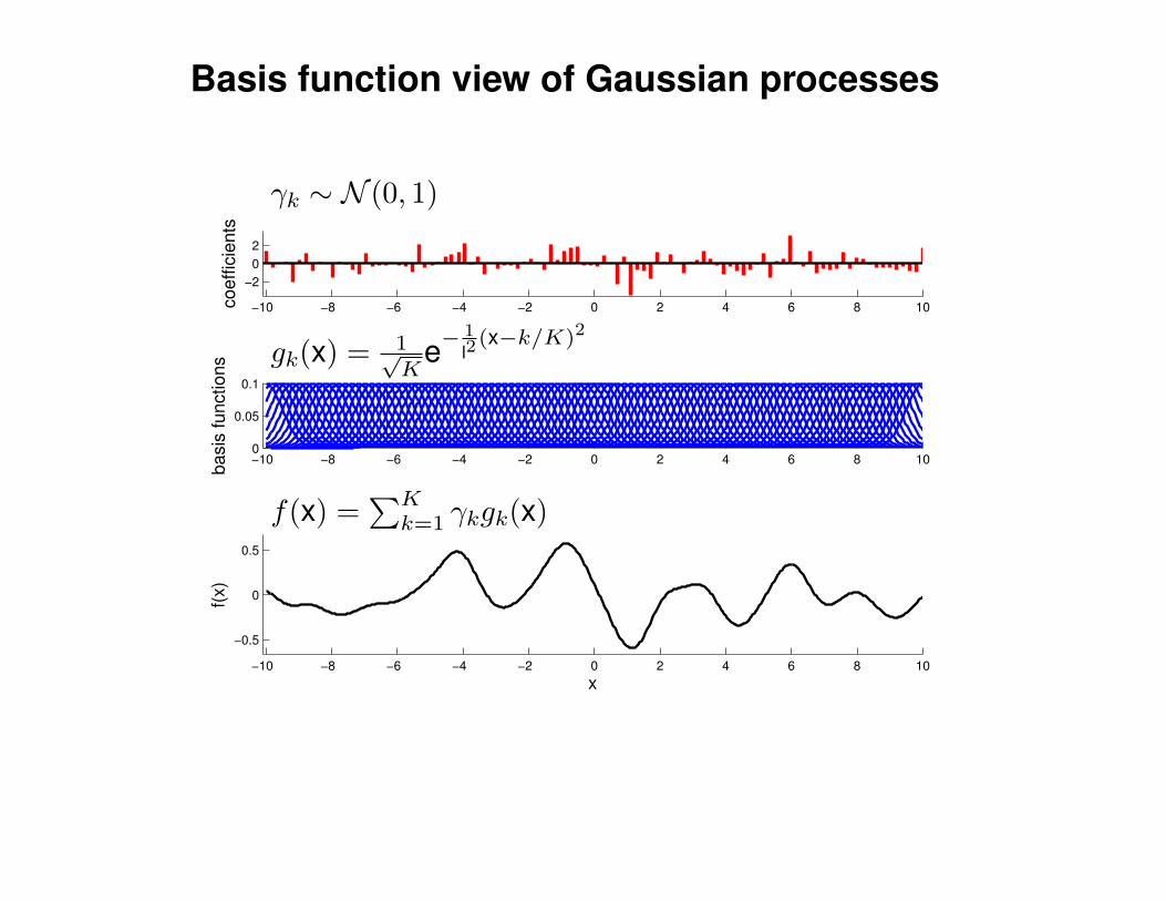
Basis function view of Gaussian processes
−10 −8 −6 −4 −2 0 2 4 6 8 10
−2
0
2
co
eff
icie
nts
−10 −8 −6 −4 −2 0 2 4 6 8 100
0.05
0.1
ba
sis
fu
nctio
ns
−10 −8 −6 −4 −2 0 2 4 6 8 10
−0.5
0
0.5
x
f(x)
γk ∼ N (0, 1)
gk(x) = 1√K
e−1
l2(x−k/K)2
f(x) =∑Kk=1 γkgk(x)
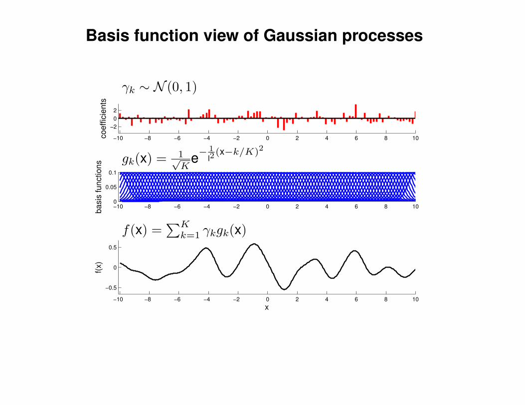
Basis function view of Gaussian processes
−10 −8 −6 −4 −2 0 2 4 6 8 10
−2
0
2
co
eff
icie
nts
−10 −8 −6 −4 −2 0 2 4 6 8 100
0.05
0.1
ba
sis
fu
nctio
ns
−10 −8 −6 −4 −2 0 2 4 6 8 10
−0.5
0
0.5
x
f(x)
γk ∼ N (0, 1)
gk(x) = 1√K
e−1
l2(x−k/K)2
f(x) =∑Kk=1 γkgk(x)
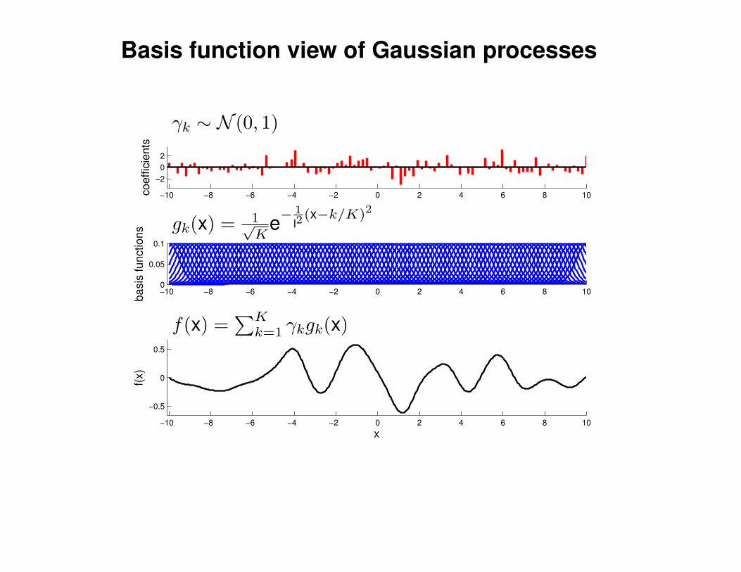
Basis function view of Gaussian processes
−10 −8 −6 −4 −2 0 2 4 6 8 10
−2
0
2
co
eff
icie
nts
−10 −8 −6 −4 −2 0 2 4 6 8 100
0.05
0.1
ba
sis
fu
nctio
ns
−10 −8 −6 −4 −2 0 2 4 6 8 10
−0.5
0
0.5
x
f(x)
γk ∼ N (0, 1)
gk(x) = 1√K
e−1
l2(x−k/K)2
f(x) =∑Kk=1 γkgk(x)
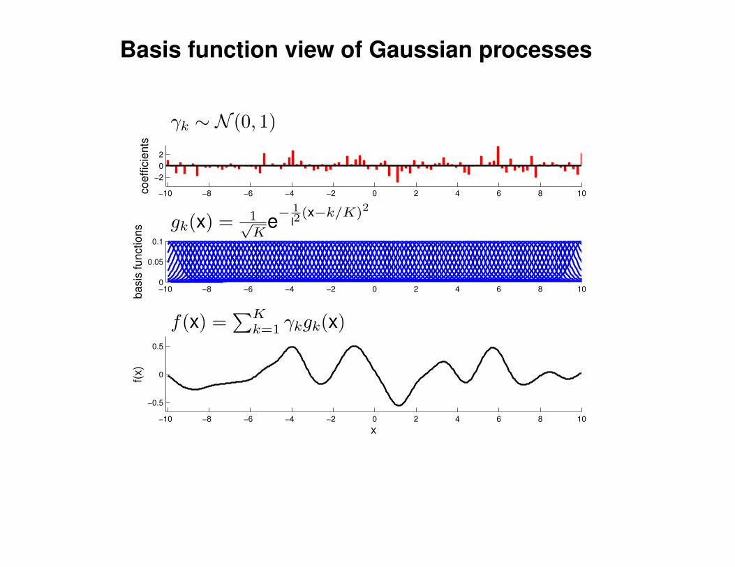
Basis function view of Gaussian processes
−10 −8 −6 −4 −2 0 2 4 6 8 10
−2
0
2
co
eff
icie
nts
−10 −8 −6 −4 −2 0 2 4 6 8 100
0.05
0.1
ba
sis
fu
nctio
ns
−10 −8 −6 −4 −2 0 2 4 6 8 10
−0.5
0
0.5
x
f(x)
γk ∼ N (0, 1)
gk(x) = 1√K
e−1
l2(x−k/K)2
f(x) =∑Kk=1 γkgk(x)

Basis function view of Gaussian processes
−10 −8 −6 −4 −2 0 2 4 6 8 10
−2
0
2
co
eff
icie
nts
−10 −8 −6 −4 −2 0 2 4 6 8 100
0.05
0.1
ba
sis
fu
nctio
ns
−10 −8 −6 −4 −2 0 2 4 6 8 10
−0.5
0
0.5
x
f(x)
γk ∼ N (0, 1)
gk(x) = 1√K
e−1
l2(x−k/K)2
f(x) =∑Kk=1 γkgk(x)
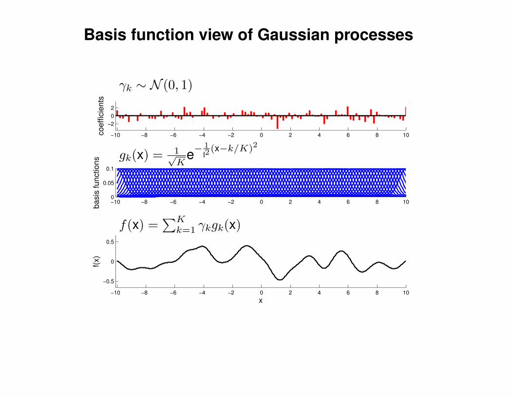
Basis function view of Gaussian processes
−10 −8 −6 −4 −2 0 2 4 6 8 10
−2
0
2
co
eff
icie
nts
−10 −8 −6 −4 −2 0 2 4 6 8 100
0.05
0.1
ba
sis
fu
nctio
ns
−10 −8 −6 −4 −2 0 2 4 6 8 10
−0.5
0
0.5
x
f(x)
γk ∼ N (0, 1)
gk(x) = 1√K
e−1
l2(x−k/K)2
f(x) =∑Kk=1 γkgk(x)

Basis function view of Gaussian processes
−10 −8 −6 −4 −2 0 2 4 6 8 10
−0.5
0
0.5
x
f(x)
γk ∼ N (0, 1)
gk(x) = 1√K
e−1
l2(x−k/K)2
f(x) =∑Kk=1 γkgk(x)
m(x) = 〈f(x)〉
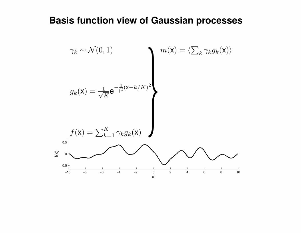
Basis function view of Gaussian processes
−10 −8 −6 −4 −2 0 2 4 6 8 10
−0.5
0
0.5
x
f(x)
γk ∼ N (0, 1)
gk(x) = 1√K
e−1
l2(x−k/K)2
f(x) =∑Kk=1 γkgk(x)
m(x) = 〈∑k γkgk(x)〉

Basis function view of Gaussian processes
−10 −8 −6 −4 −2 0 2 4 6 8 10
−0.5
0
0.5
x
f(x)
γk ∼ N (0, 1)
gk(x) = 1√K
e−1
l2(x−k/K)2
f(x) =∑Kk=1 γkgk(x)
m(x) =∑k〈γk〉gk(x)
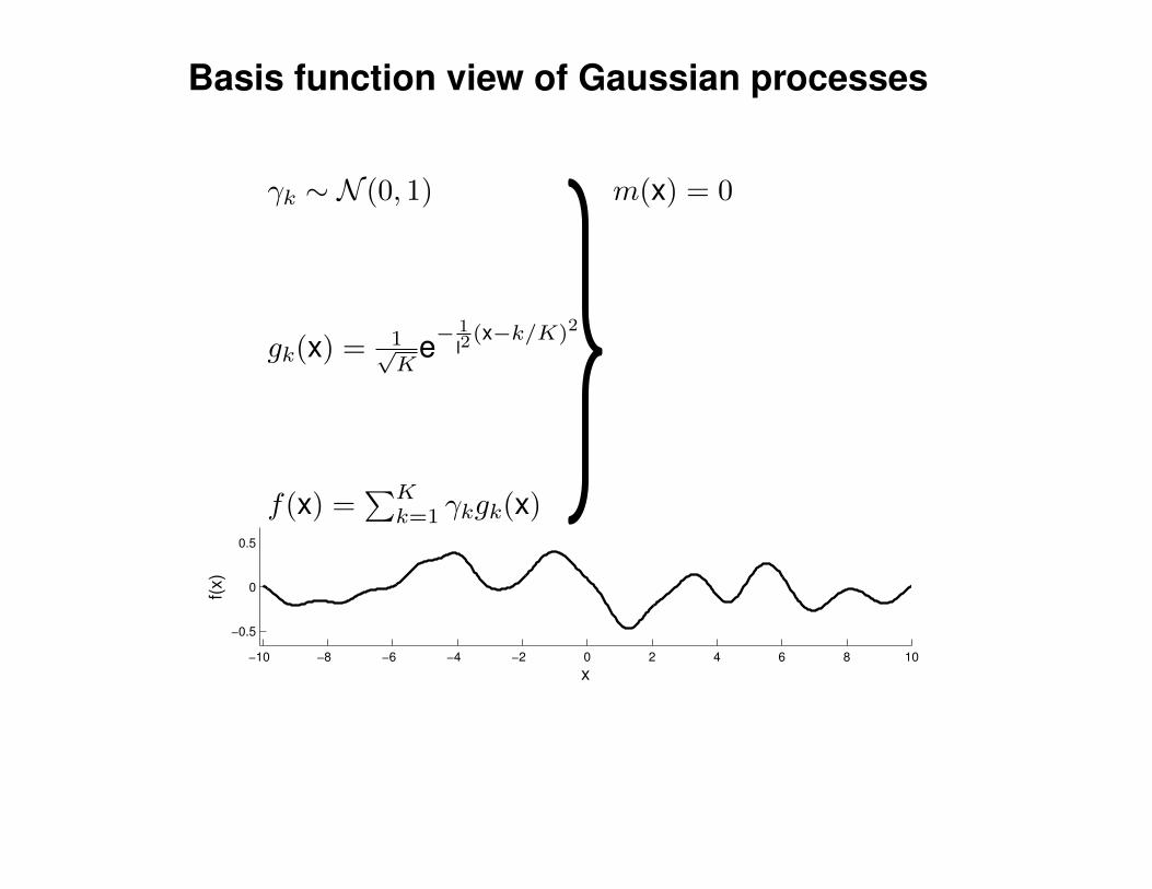
Basis function view of Gaussian processes
−10 −8 −6 −4 −2 0 2 4 6 8 10
−0.5
0
0.5
x
f(x)
γk ∼ N (0, 1)
gk(x) = 1√K
e−1
l2(x−k/K)2
f(x) =∑Kk=1 γkgk(x)
m(x) = 0
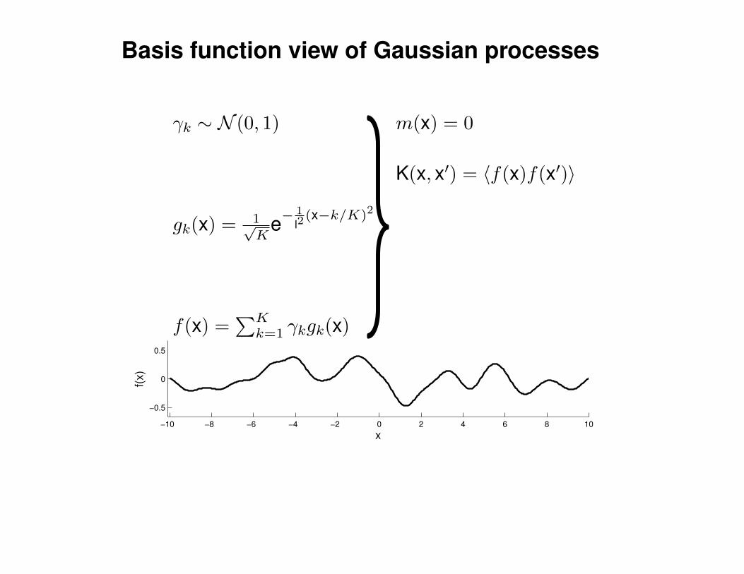
Basis function view of Gaussian processes
−10 −8 −6 −4 −2 0 2 4 6 8 10
−0.5
0
0.5
x
f(x)
γk ∼ N (0, 1)
gk(x) = 1√K
e−1
l2(x−k/K)2
f(x) =∑Kk=1 γkgk(x)
m(x) = 0
K(x, x′) = 〈f(x)f(x′)〉
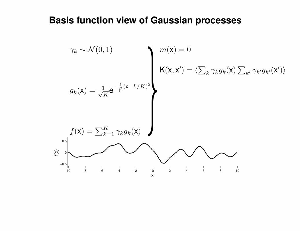
Basis function view of Gaussian processes
−10 −8 −6 −4 −2 0 2 4 6 8 10
−0.5
0
0.5
x
f(x)
γk ∼ N (0, 1)
gk(x) = 1√K
e−1
l2(x−k/K)2
f(x) =∑Kk=1 γkgk(x)
m(x) = 0
K(x, x′) = 〈∑k γkgk(x)
∑k′ γk′gk′(x
′)〉
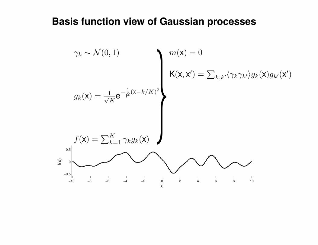
Basis function view of Gaussian processes
−10 −8 −6 −4 −2 0 2 4 6 8 10
−0.5
0
0.5
x
f(x)
γk ∼ N (0, 1)
gk(x) = 1√K
e−1
l2(x−k/K)2
f(x) =∑Kk=1 γkgk(x)
m(x) = 0
K(x, x′) =∑k,k′〈γkγk′〉gk(x)gk′(x′)

Basis function view of Gaussian processes
−10 −8 −6 −4 −2 0 2 4 6 8 10
−0.5
0
0.5
x
f(x)
γk ∼ N (0, 1)
gk(x) = 1√K
e−1
l2(x−k/K)2
f(x) =∑Kk=1 γkgk(x)
m(x) = 0
K(x, x′) =∑k,k′ δk,k′gk(x)gk′(x′)
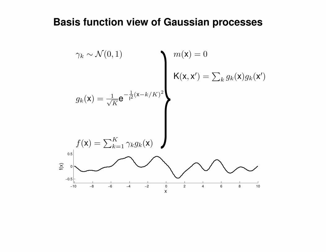
Basis function view of Gaussian processes
−10 −8 −6 −4 −2 0 2 4 6 8 10
−0.5
0
0.5
x
f(x)
γk ∼ N (0, 1)
gk(x) = 1√K
e−1
l2(x−k/K)2
f(x) =∑Kk=1 γkgk(x)
m(x) = 0
K(x, x′) =∑k gk(x)gk(x′)
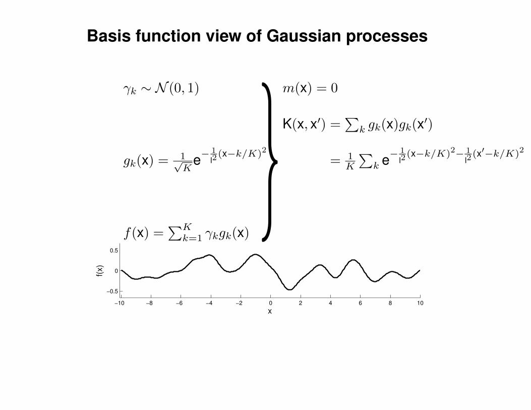
Basis function view of Gaussian processes
−10 −8 −6 −4 −2 0 2 4 6 8 10
−0.5
0
0.5
x
f(x)
γk ∼ N (0, 1)
gk(x) = 1√K
e−1
l2(x−k/K)2
f(x) =∑Kk=1 γkgk(x)
m(x) = 0
K(x, x′) =∑k gk(x)gk(x′)
K(x, x′) = 1K
∑k e−
1
l2(x−k/K)2− 1
l2(x′−k/K)2
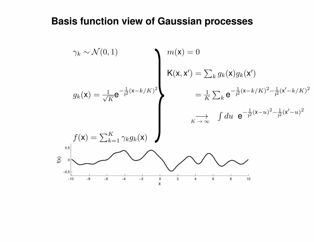
Basis function view of Gaussian processes
−10 −8 −6 −4 −2 0 2 4 6 8 10
−0.5
0
0.5
x
f(x)
γk ∼ N (0, 1)
gk(x) = 1√K
e−1
l2(x−k/K)2
f(x) =∑Kk=1 γkgk(x)
m(x) = 0
K(x, x′) =∑k gk(x)gk(x′)
K(x, x′) = 1K
∑k e−
1
l2(x−k/K)2− 1
l2(x′−k/K)2
K(x, x′) −→∫du e−
1
l2(x−u)2− 1
l2(x′−u)2
K →∞
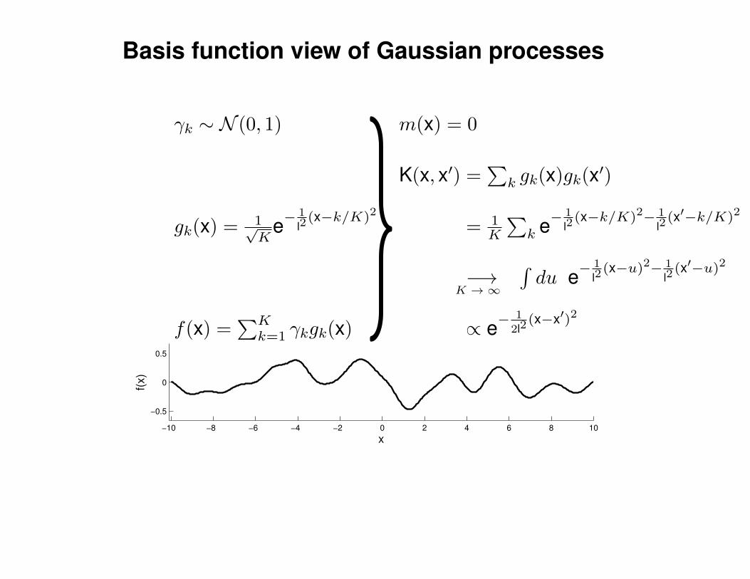
Basis function view of Gaussian processes
−10 −8 −6 −4 −2 0 2 4 6 8 10
−0.5
0
0.5
x
f(x)
γk ∼ N (0, 1)
gk(x) = 1√K
e−1
l2(x−k/K)2
f(x) =∑Kk=1 γkgk(x)
m(x) = 0
K(x, x′) =∑k gk(x)gk(x′)
K(x, x′) = 1K
∑k e−
1
l2(x−k/K)2− 1
l2(x′−k/K)2
K(x, x′) −→∫du e−
1
l2(x−u)2− 1
l2(x′−u)2
K →∞
K(x, x′) ∝ e−1
2l2(x−x′)2
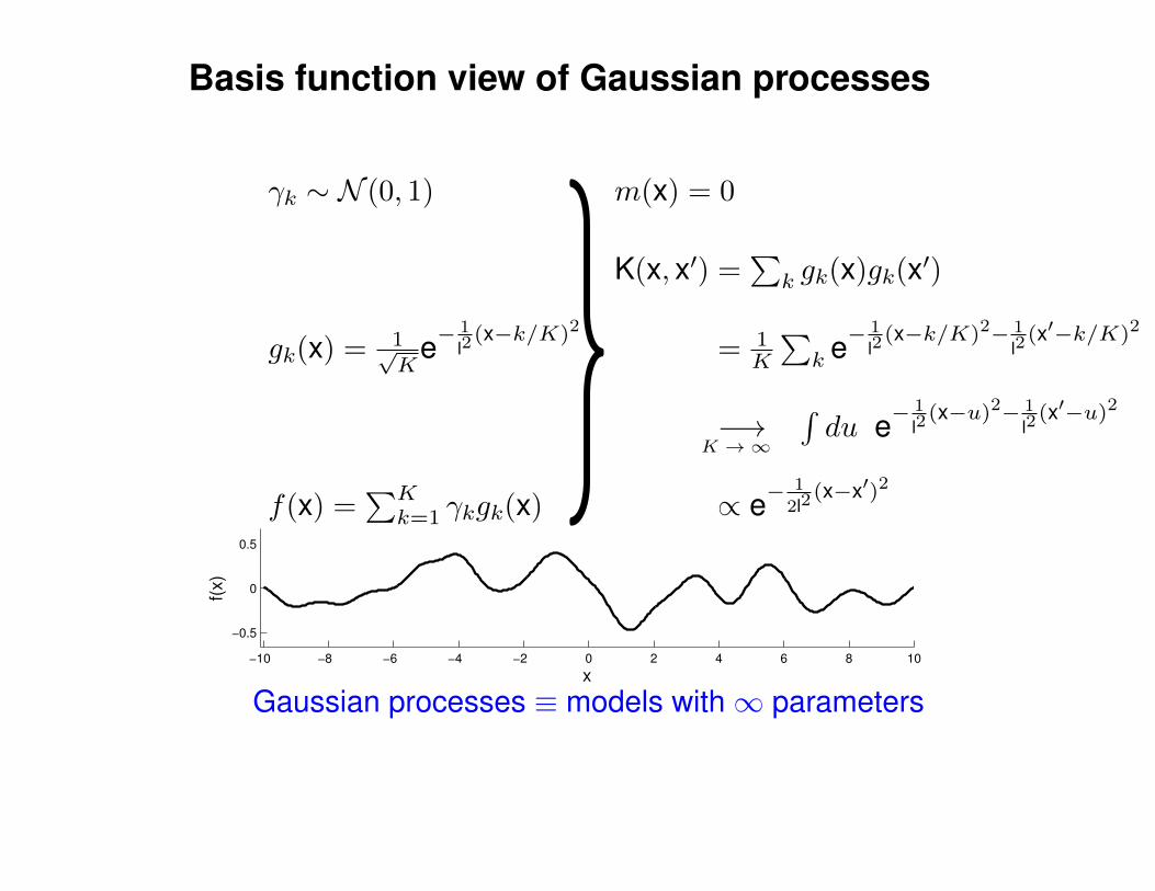
Gaussian processes ≡ models with∞ parameters
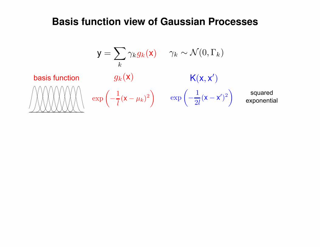
Basis function view of Gaussian Processes
basis function
squaredexponential
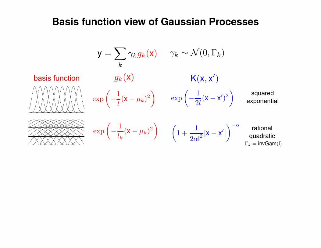
Basis function view of Gaussian Processes
basis function
rationalquadratic
squaredexponential
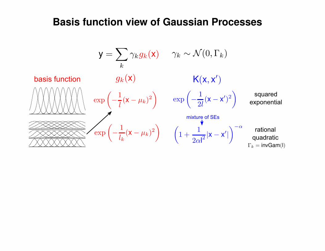
Basis function view of Gaussian Processes
basis function
rationalquadratic
squaredexponential
mixture of SEs
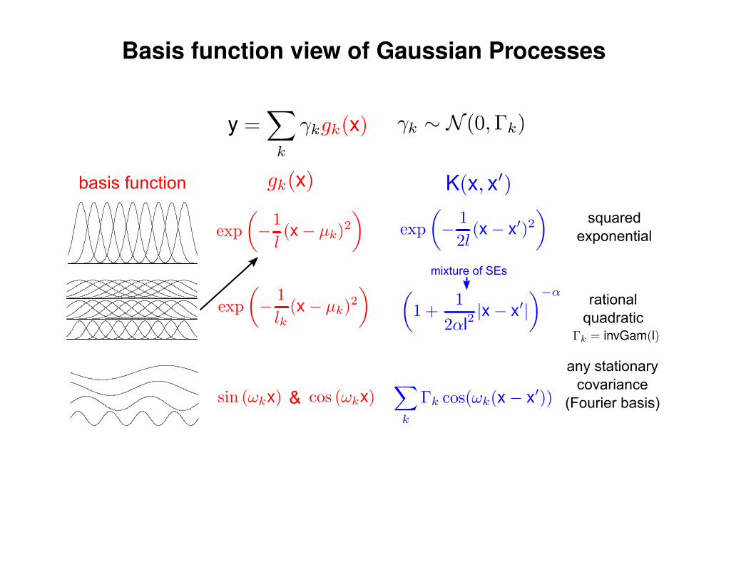
Basis function view of Gaussian Processes
&
basis function
rationalquadratic
squaredexponential
any stationarycovariance
(Fourier basis)
mixture of SEs
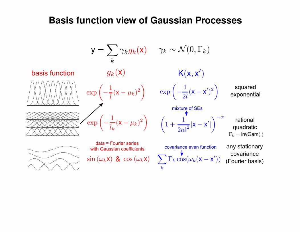
Basis function view of Gaussian Processes
&
basis function
rationalquadratic
squaredexponential
any stationarycovariance
(Fourier basis)
covariance even functiondata = Fourier series
with Gaussian coefficients
mixture of SEs
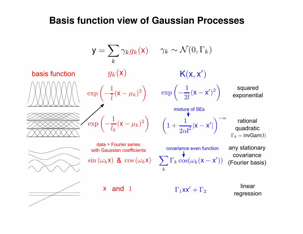
Basis function view of Gaussian Processes
&
basis function
and
rationalquadratic
squaredexponential
any stationarycovariance
(Fourier basis)
linear regression
covariance even functiondata = Fourier series
with Gaussian coefficients
mixture of SEs
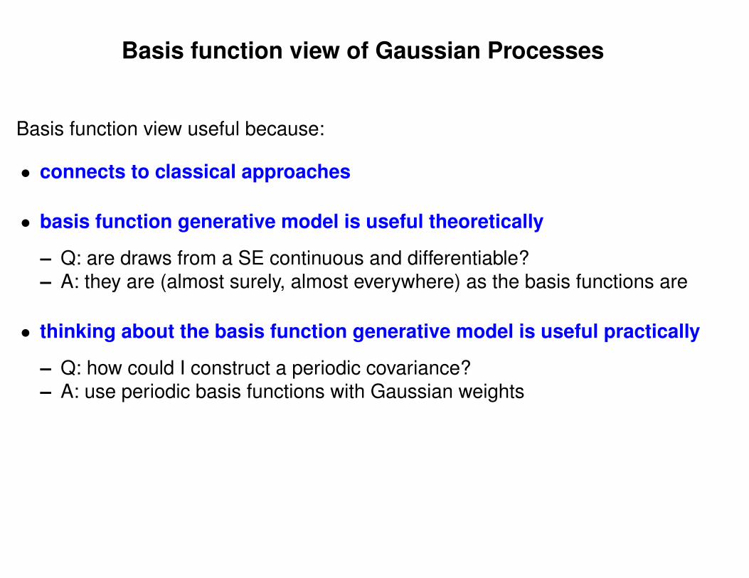
Basis function view of Gaussian Processes
Basis function view useful because:
• connects to classical approaches
• basis function generative model is useful theoretically
– Q: are draws from a SE continuous and differentiable?– A: they are (almost surely, almost everywhere) as the basis functions are
• thinking about the basis function generative model is useful practically
– Q: how could I construct a periodic covariance?– A: use periodic basis functions with Gaussian weights
Making new covariance functions from old
(positive) linear combinationsof covariance functions
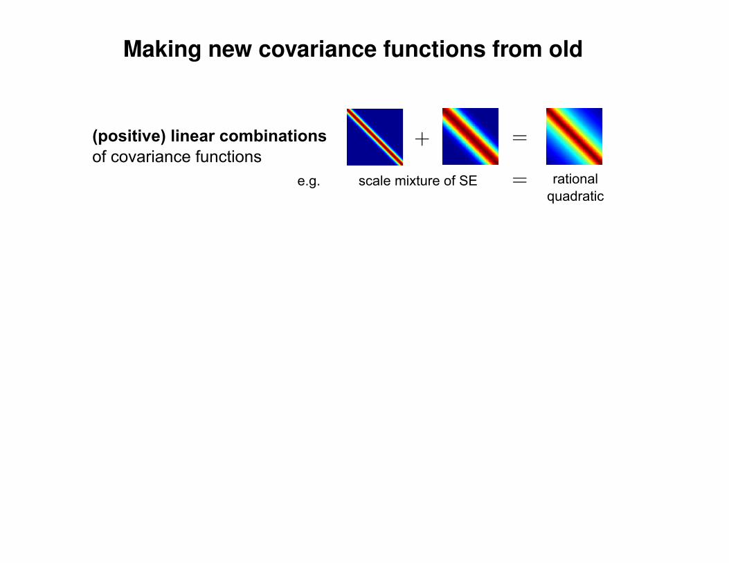
Making new covariance functions from old
(positive) linear combinationsof covariance functions
e.g. scale mixture of SE rationalquadratic
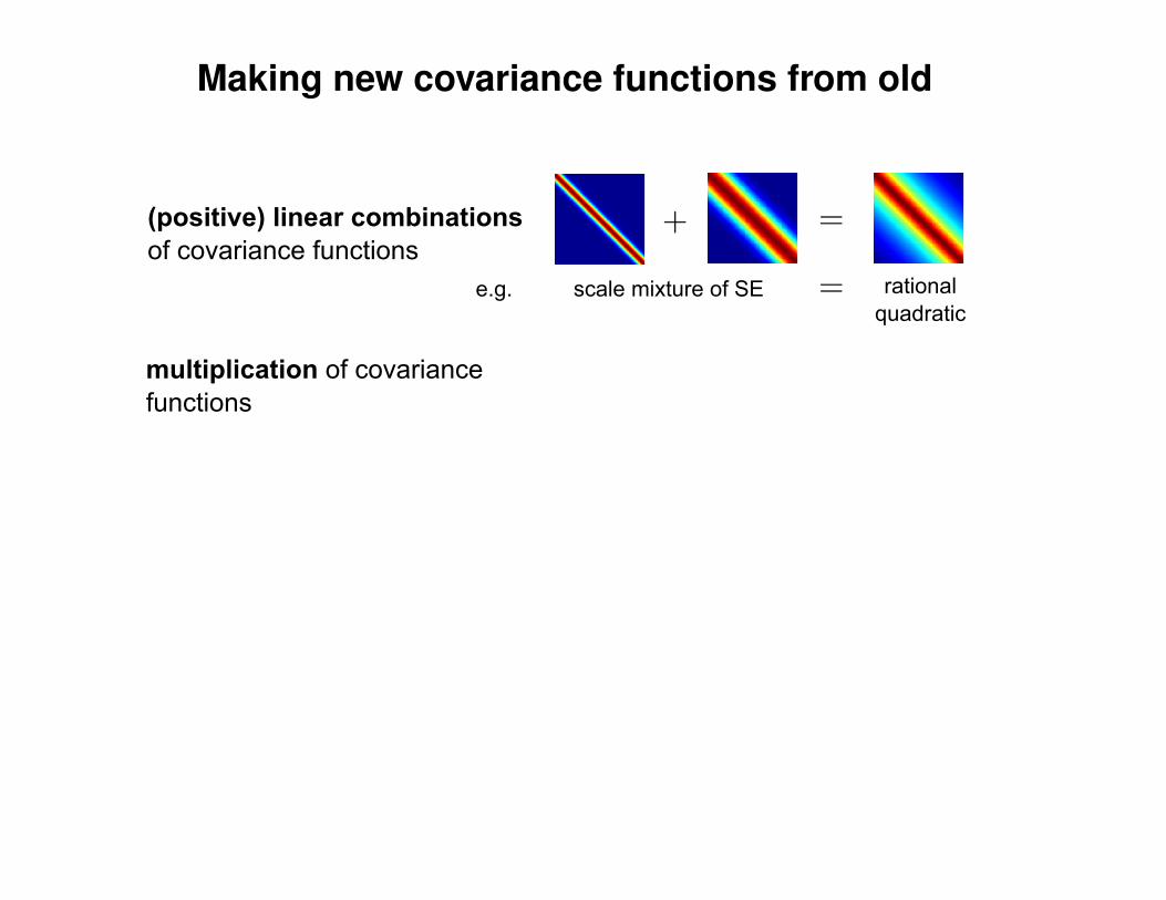
Making new covariance functions from old
(positive) linear combinationsof covariance functions
multiplication of covariancefunctions
e.g. scale mixture of SE rationalquadratic
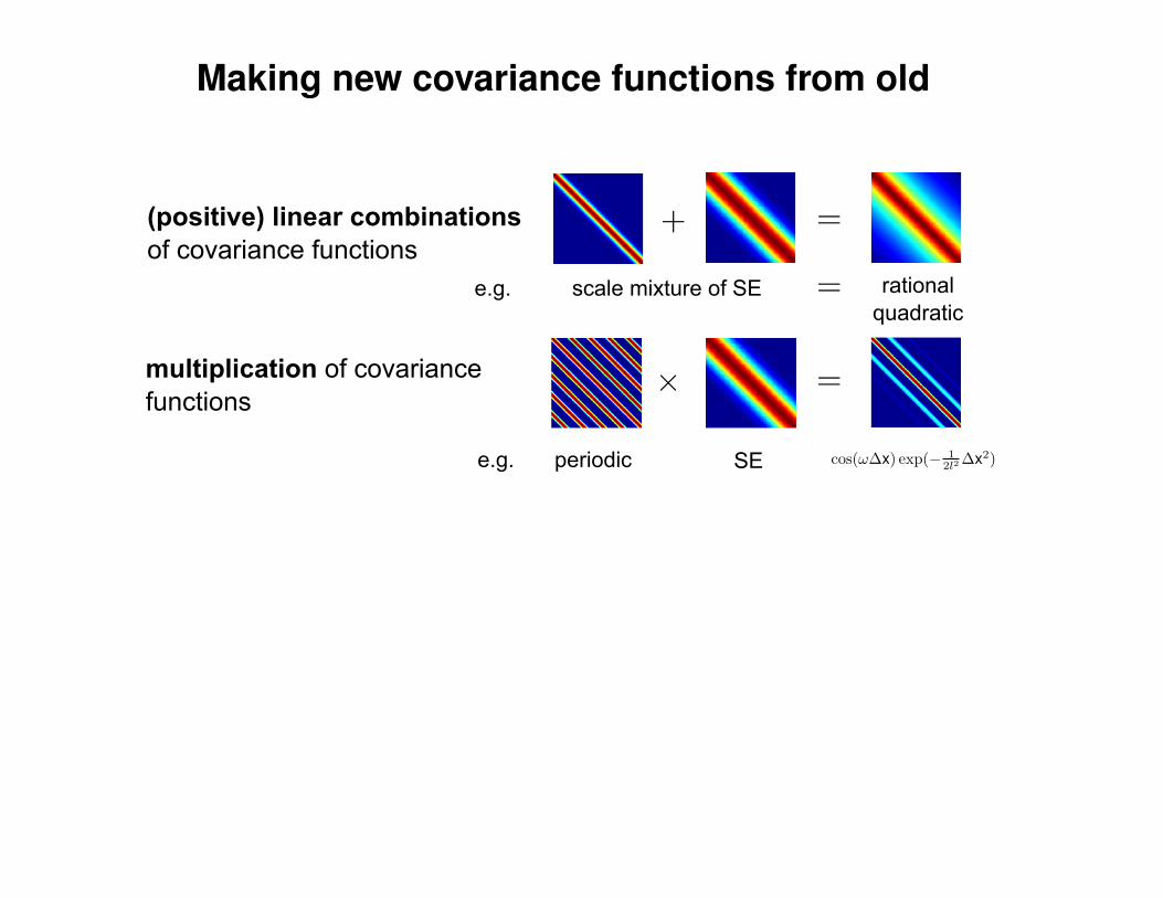
Making new covariance functions from old
(positive) linear combinationsof covariance functions
multiplication of covariancefunctions
e.g. scale mixture of SE rationalquadratic
e.g. periodic SE
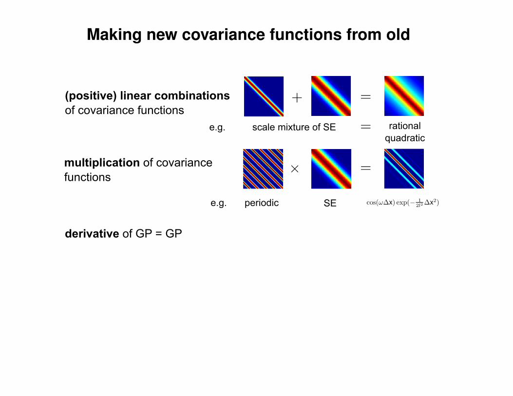
Making new covariance functions from old
(positive) linear combinationsof covariance functions
multiplication of covariancefunctions
e.g. scale mixture of SE
derivative of GP = GP
rationalquadratic
e.g. periodic SE
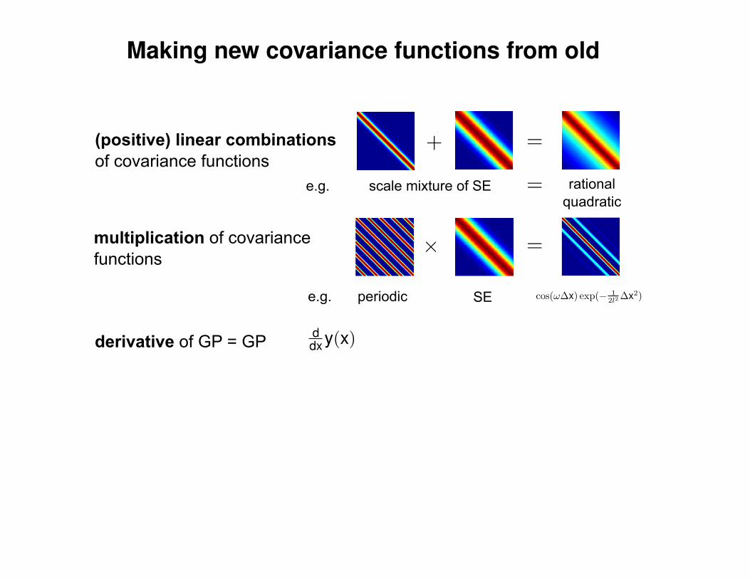
Making new covariance functions from old
(positive) linear combinationsof covariance functions
multiplication of covariancefunctions
e.g. scale mixture of SE
derivative of GP = GP
rationalquadratic
e.g. periodic SE
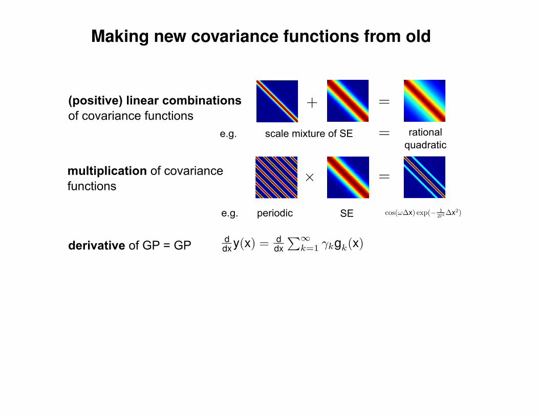
Making new covariance functions from old
(positive) linear combinationsof covariance functions
multiplication of covariancefunctions
e.g. scale mixture of SE
derivative of GP = GP
rationalquadratic
e.g. periodic SE
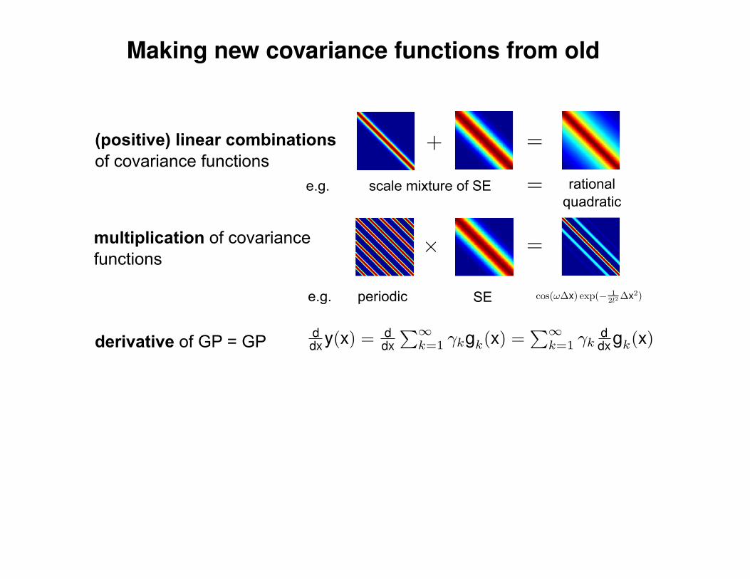
Making new covariance functions from old
(positive) linear combinationsof covariance functions
multiplication of covariancefunctions
e.g. scale mixture of SE
derivative of GP = GP
rationalquadratic
e.g. periodic SE
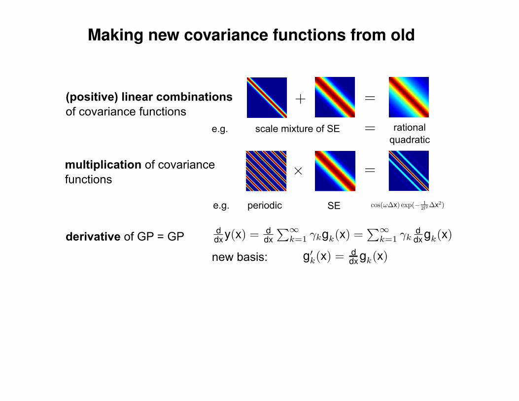
Making new covariance functions from old
(positive) linear combinationsof covariance functions
multiplication of covariancefunctions
e.g. scale mixture of SE
derivative of GP = GP
rationalquadratic
e.g. periodic SE
new basis:
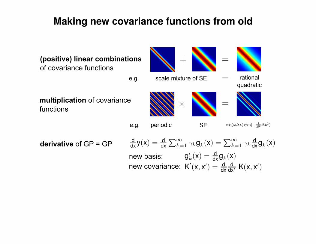
Making new covariance functions from old
(positive) linear combinationsof covariance functions
multiplication of covariancefunctions
e.g. scale mixture of SE
derivative of GP = GP
rationalquadratic
e.g. periodic SE
new basis:new covariance:
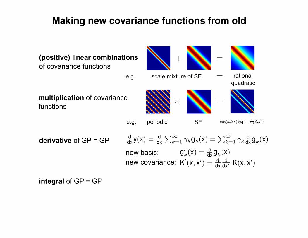
Making new covariance functions from old
(positive) linear combinationsof covariance functions
multiplication of covariancefunctions
e.g. scale mixture of SE
derivative of GP = GP
integral of GP = GP
rationalquadratic
e.g. periodic SE
new basis:new covariance:

Making new covariance functions from old
(positive) linear combinationsof covariance functions
multiplication of covariancefunctions
e.g. scale mixture of SE
derivative of GP = GP
integral of GP = GP
rationalquadratic
e.g. periodic SE
new basis:new covariance:
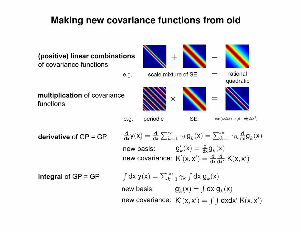
Making new covariance functions from old
(positive) linear combinationsof covariance functions
multiplication of covariancefunctions
e.g. scale mixture of SE
derivative of GP = GP
integral of GP = GP
rationalquadratic
e.g. periodic SE
new basis:
new basis:
new covariance:
new covariance:
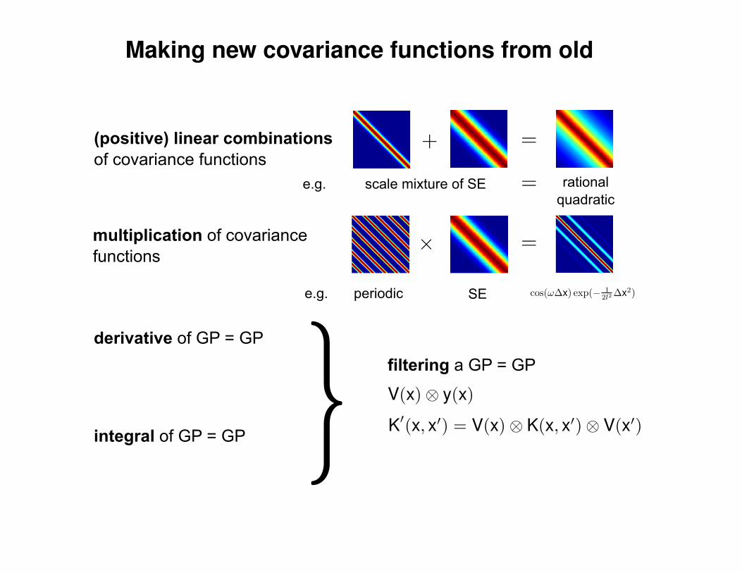
Making new covariance functions from old
(positive) linear combinationsof covariance functions
multiplication of covariancefunctions
e.g. scale mixture of SE
derivative of GP = GP
integral of GP = GP
rationalquadratic
e.g. periodic SE
filtering a GP = GP
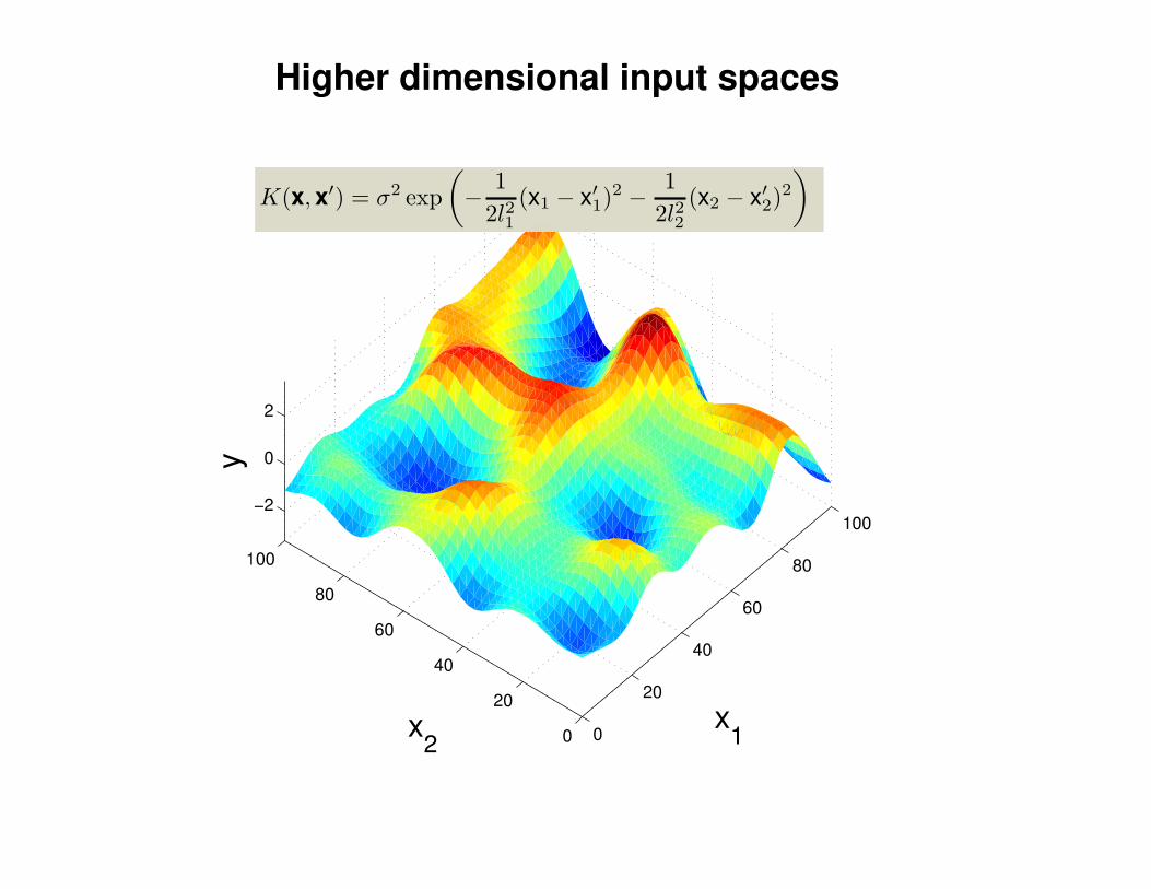
Higher dimensional input spaces
0
20
40
60
80
100
0
20
40
60
80
100
−2
0
2
x1x
2
y
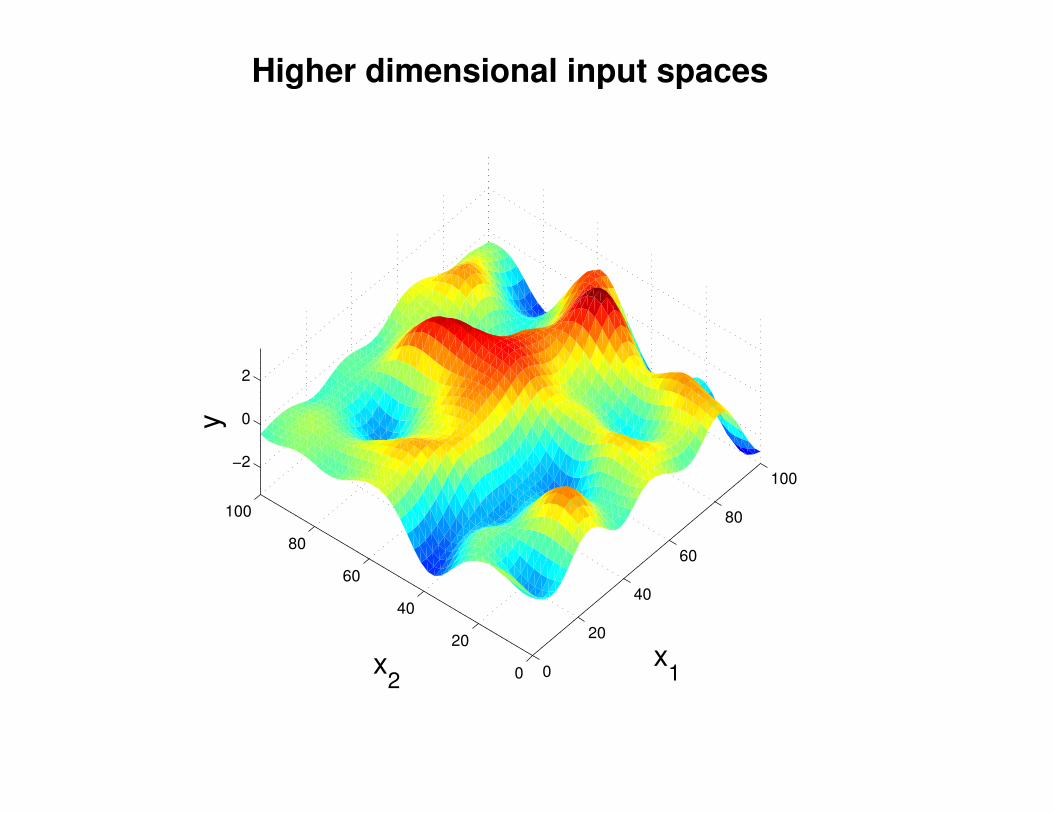
Higher dimensional input spaces
0
20
40
60
80
100
0
20
40
60
80
100
−2
0
2
x1x
2
y
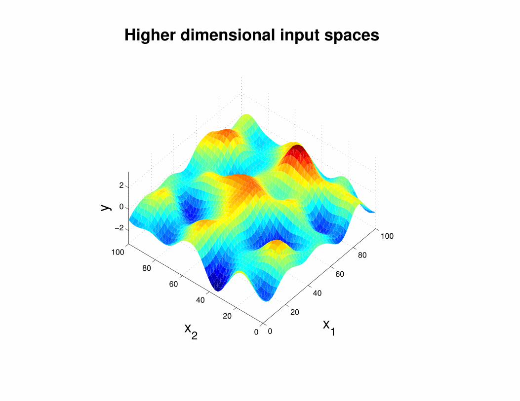
Higher dimensional input spaces
0
20
40
60
80
100
0
20
40
60
80
100
−2
0
2
x1x
2
y
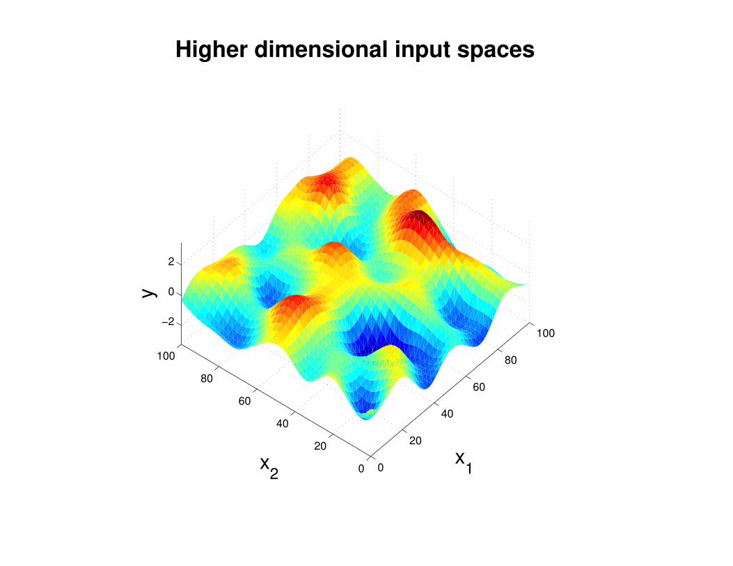
Higher dimensional input spaces
0
20
40
60
80
100
0
20
40
60
80
100
−2
0
2
x1x
2
y
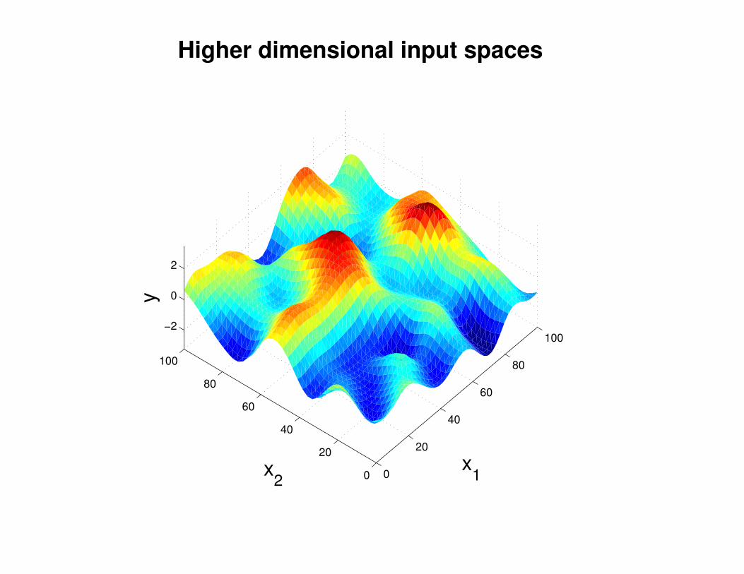
Higher dimensional input spaces
0
20
40
60
80
100
0
20
40
60
80
100
−2
0
2
x1x
2
y
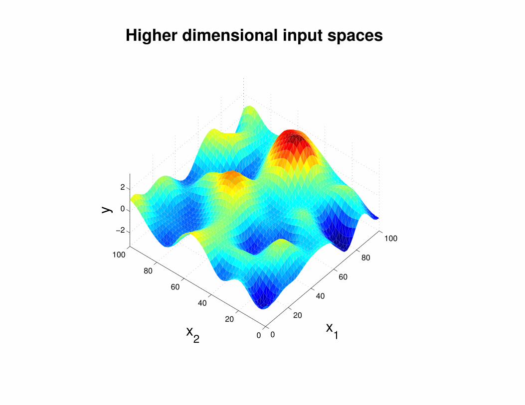
Higher dimensional input spaces
0
20
40
60
80
100
0
20
40
60
80
100
−2
0
2
x1x
2
y
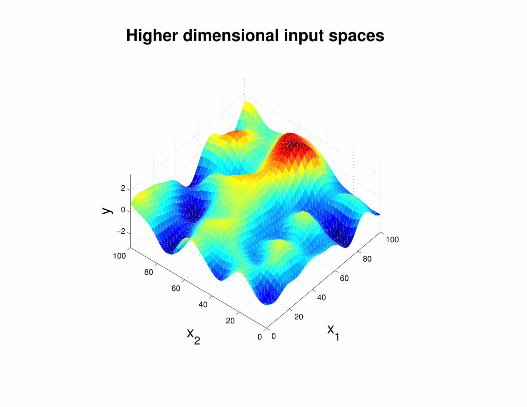
Higher dimensional input spaces
0
20
40
60
80
100
0
20
40
60
80
100
−2
0
2
x1x
2
y
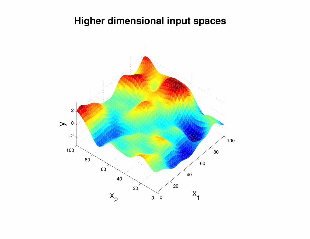
Higher dimensional input spaces
0
20
40
60
80
100
0
20
40
60
80
100
−2
0
2
x1x
2
y
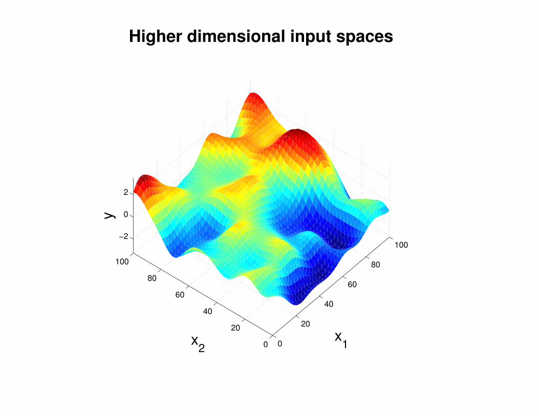
Higher dimensional input spaces
0
20
40
60
80
100
0
20
40
60
80
100
−2
0
2
x1x
2
y
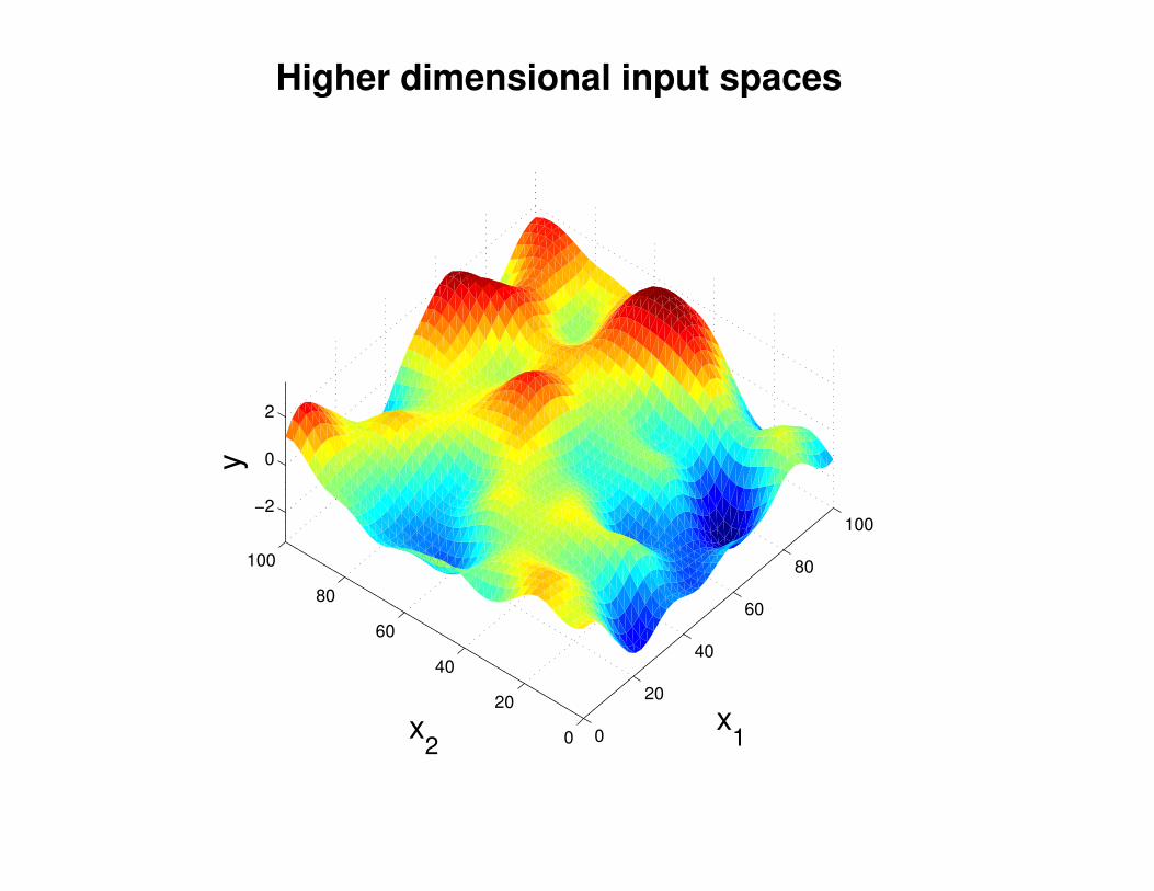
Higher dimensional input spaces
0
20
40
60
80
100
0
20
40
60
80
100
−2
0
2
x1x
2
y
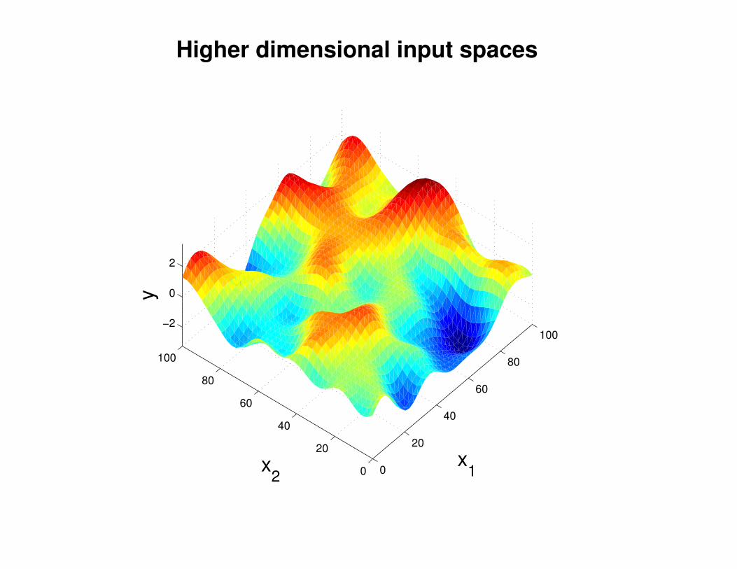
Higher dimensional input spaces
0
20
40
60
80
100
0
20
40
60
80
100
−2
0
2
x1x
2
y
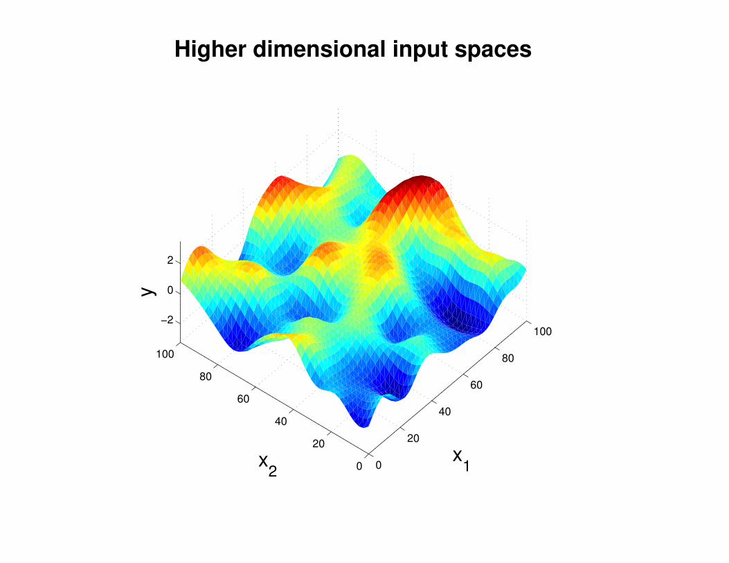
Higher dimensional input spaces
0
20
40
60
80
100
0
20
40
60
80
100
−2
0
2
x1x
2
y
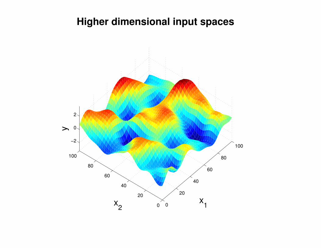
Higher dimensional input spaces
0
20
40
60
80
100
0
20
40
60
80
100
−2
0
2
x1x
2
y
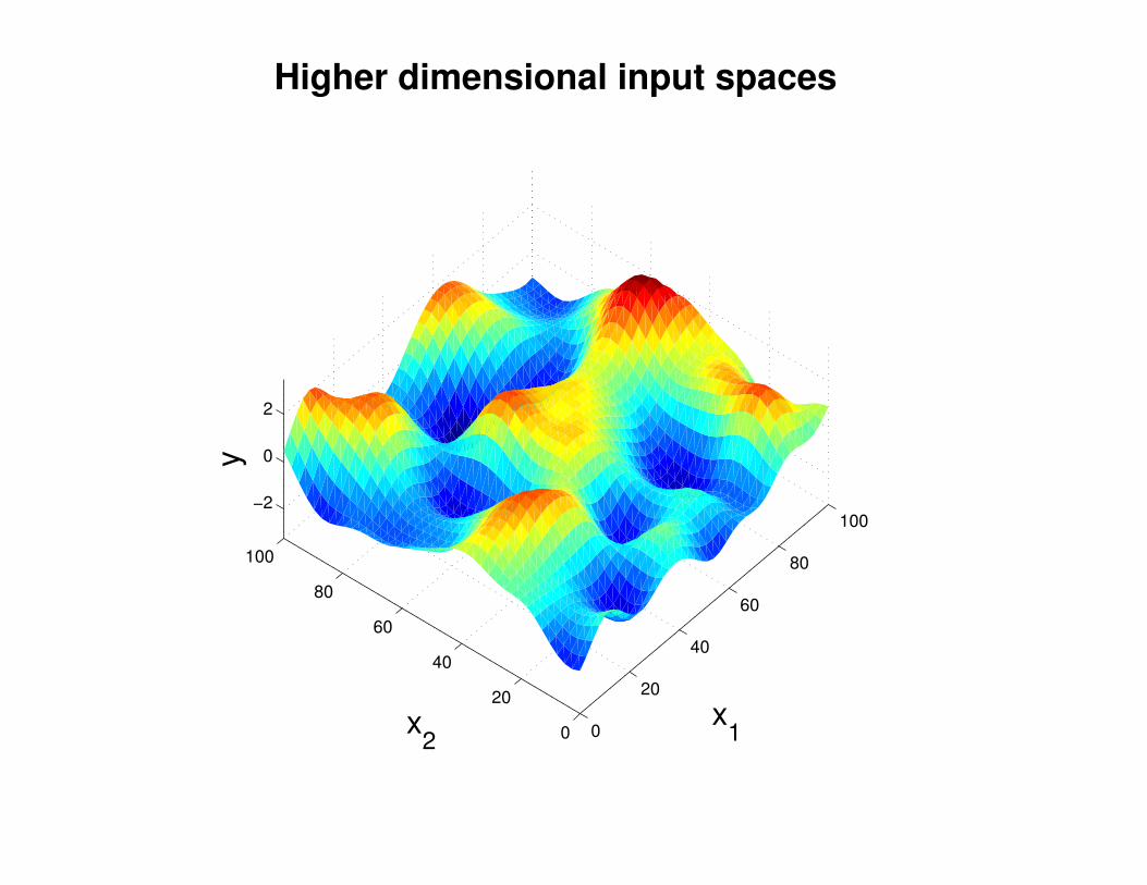
Higher dimensional input spaces
0
20
40
60
80
100
0
20
40
60
80
100
−2
0
2
x1x
2
y
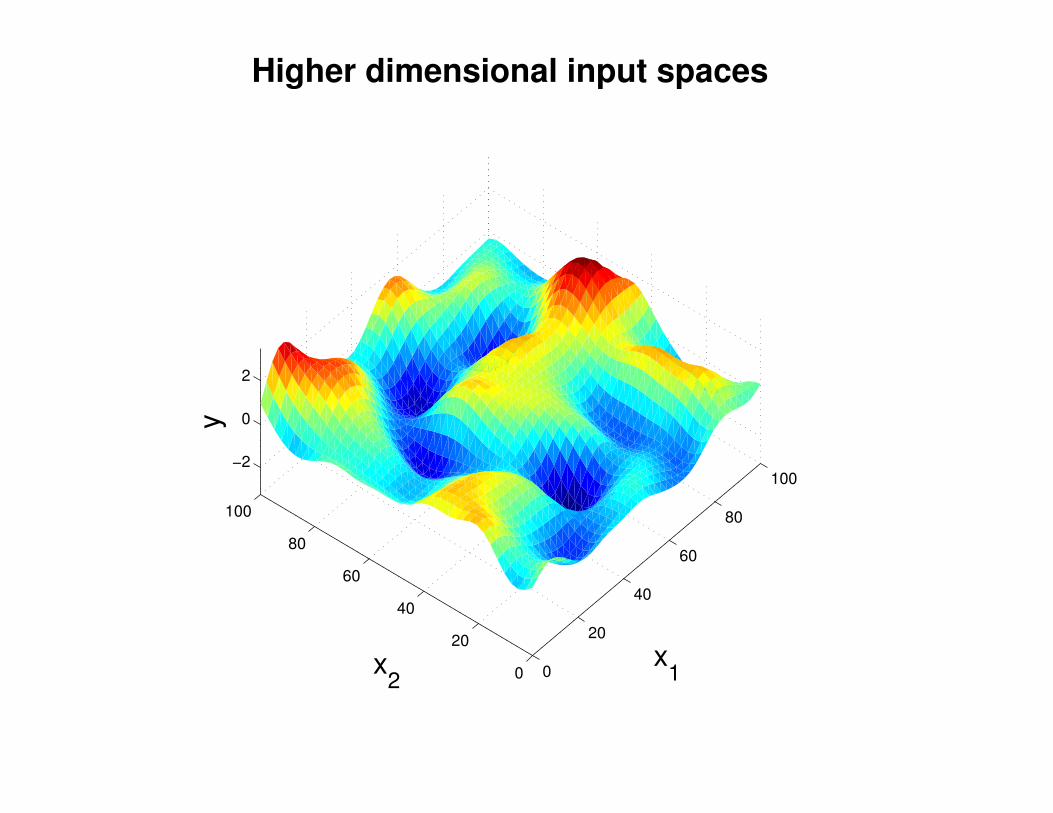
Higher dimensional input spaces
0
20
40
60
80
100
0
20
40
60
80
100
−2
0
2
x1x
2
y
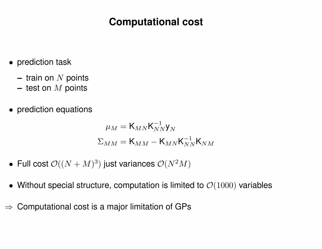
Computational cost
• prediction task
– train on N points– test on M points
• prediction equations
µM = KMNK−1NNyN
ΣMM = KMM − KMNK−1NNKNM
• Full cost O((N +M)3) just variances O(N2M)
• Without special structure, computation is limited to O(1000) variables
⇒ Computational cost is a major limitation of GPs
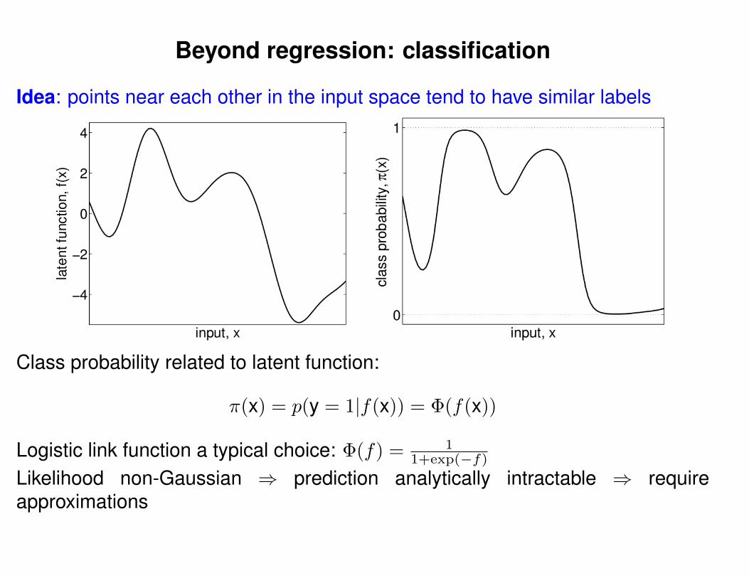
Beyond regression: classification
Idea: points near each other in the input space tend to have similar labels
Class probability related to latent function:
π(x) = p(y = 1|f(x)) = Φ(f(x))
Logistic link function a typical choice: Φ(f) = 11+exp(−f)
Likelihood non-Gaussian ⇒ prediction analytically intractable ⇒ requireapproximations
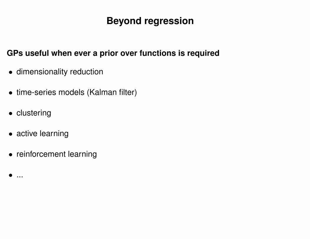
Beyond regression
GPs useful when ever a prior over functions is required
• dimensionality reduction
• time-series models (Kalman filter)
• clustering
• active learning
• reinforcement learning
• ...
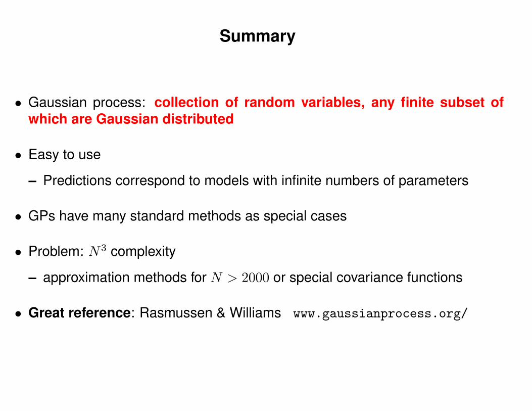
Summary
• Gaussian process: collection of random variables, any finite subset ofwhich are Gaussian distributed
• Easy to use
– Predictions correspond to models with infinite numbers of parameters
• GPs have many standard methods as special cases
• Problem: N3 complexity
– approximation methods for N > 2000 or special covariance functions
• Great reference: Rasmussen & Williams www.gaussianprocess.org/