Shear band localization via local J continuum damage mechanics

Comput. Methods Appl. Mech. Engrg. 193 (2004) 849–880

www.elsevier.com/locate/cma

Shear band localization via local J2 continuumdamage mechanics

M. Cervera *, M. Chiumenti, C. Agelet de Saracibar

International Center for Numerical Methods in Engineering (CIMNE), Technical University of Catalonia (UPC), Edificio C1,

Campus Norte, Jordi Girona 1–3, Barcelona 08034, Spain

Received 21 July 2003; received in revised form 29 October 2003; accepted 10 November 2003

Abstract

This paper describes a novel formulation for the solution of problems involving shear band localization using a local

isotropic J2 continuum damage model and mixed linear simplex (triangles and tetrahedra). Stabilization methods are

used to ensure existence and uniqueness of the solution, attaining global and local stability of the corresponding discrete

finite element formulation. Consistent residual viscosity is used to enhance robustness and convergence of the for-

mulation. Implementation and computational aspects are also discussed. A simple isotropic local J2 damage consti-

tutive model is considered, either with linear or exponential softening. The softening modulus is regularized according

to the material mode II fracture energy and the element size. Numerical examples show that the formulation derived is

fully stable and remarkably robust, totally free of volumetric locking and spurious oscillations of the pressure. As a

consequence, the results obtained do not suffer from spurious mesh-size or mesh-bias dependence, comparing very

favourably with those obtained with the ill-posed standard approaches.

� 2004 Elsevier B.V. All rights reserved.

Keywords: Shear bands; Softening; Localization and stabilization; Damage; Incompressibility

1. Introduction

It is well established that softening materials subjected to monotonic straining exhibit strain localization.

In particular, in the so-called J2 materials, shear (or slip) strains concentrate, under certain circumstances.

This phenomenon leads to the formation of shear bands inside the solid where, once the peak stress is

reached, the deformation concentrates while the material outside the band unloads. This induces the for-

mation of weak discontinuities, with continuous fields of slip displacements but discontinuous fields of shearstrain inside and outside the bands (see Fig. 1a, where u denotes slip displacement and e denotes deviatoricstrain values).

* Corresponding author.

E-mail address: [email protected] (M. Cervera).

0045-7825/$ - see front matter � 2004 Elsevier B.V. All rights reserved.

doi:10.1016/j.cma.2003.11.009

mail to: [email protected]

Fig. 1. Strain localization: (a) weak discontinuity and (b) strong discontinuity.

850 M. Cervera et al. / Comput. Methods Appl. Mech. Engrg. 193 (2004) 849–880

Upon continuing straining, the width of the shear band diminishes and, unless there is a physical lim-

itation, it tends to zero. Ultimately, this process may lead to strong discontinuities, with discontinuous fields

of slip displacements across the discontinuity line, and unbounded shear strains (see Fig. 1b). In J2 materials,

these are called slip lines. It is generally accepted in fracture mechanics that the amount of energy released

during the formation of a unit area of slip surface is a material property, called the mode II fracture energy.

Shear bands are typical of ductile materials such as metals, although they are also observed in granular

materials such as sands or soils. Similar deformation patterns can also appear in fiber-reinforced com-

posites subjected to compressive loading.In the last two decades, many different finite element strategies have been proposed to model discon-

tinuities and the references in the bibliography are innumerable. Despite the considerable effort devoted to

the subject, theoretical modeling and computational resolution of the strain localization process up to

structural failure have remained an open challenge in Computational Solid Mechanics.

The possibilities to model shear bands with finite elements are several, and both the weak and the strong

discontinuity approaches have been followed. In the first, the objective is to capture the shear band as

precisely as possible, with standard continuous elements. In the second, the displacement field is enhanced

with discontinuous functions so that the true slip line can be captured. In fact, both approaches arecompatible. On one hand, a weak discontinuity can be interpreted as a regularization of a strong one over a

given width, for instance with the discontinuity ‘‘smeared’’ across the maximum possible resolution of the

mesh, that is, one element; on the other hand, a strong discontinuity is the limit case of a weak one with

vanishing width.

The main difficulty why most attempts to model weak displacement discontinuities with standard, local,

approaches fail is that the solutions obtained appear to be unphysically, and unacceptably, fully determined

by the fineness and orientation of the discretization. Up to now, this disagreeable observation has been

erroneously and misleadingly attributed to the fact that, when strain-softening occurs and the slope of thelocal stress-strain curve becomes negative, the governing equations of the Continuum Mechanics problem

lose their ‘‘natural’’ elliptic character. To remedy this, many so-called ‘‘non-local’’, ‘‘gradient-enhanced’’,

‘‘micropolar’’ and ‘‘viscous-regularized’’ constitutive models have been proposed in the last decade.

In the first, non-local, strategy, the standard format of the constitutive relationships (stress at a point

depends on the strain at that point) is substituted by a non-local format (stress at a point depends on some

M. Cervera et al. / Comput. Methods Appl. Mech. Engrg. 193 (2004) 849–880 851

average measure of the strain in the neighbourhood of that point), see [1,2], among others. In the second,gradient-enhanced, strategy, a variant of the first, the nonlinear constitutive laws, for plasticity or damage,

are made dependent not only on the local inelastic strain, but also on its second gradient, which is com-

puted according to some additional relation which couples it to the local strain, [1,3–8]. In the third,

micropolar, strategy, the usual non-polar description of Continuum Mechanics is substituted by other non-

standard theory, like the Cosserat�s continuum, see, for instance, [9] and [10]. In the fourth, viscous-reg-

ularized, strategy, the rate-independent format is substituted by a regularized version, also dependent on

the strain-rate, see [1,8,11].

Even if these strategies have proved effective to some extend, they also pose new theoretical and com-putational difficulties, not fully mastered at the present moment.

Alternatively, in the last decade, an effort has been made to model numerically strong discontinuities

directly [12–14]. Again, even if the strong discontinuity concept is certainly appealing, it departs from the

usual Continuum Mechanics framework and requires a new solid theoretical basis. This leads to several

new formulations for finite elements with ‘‘embedded discontinuities’’, depending on the kinematical and

statical assumptions adopted, all of them still with open questions. For instance, the issue of uniqueness of

the solution is not fully solved yet. They also pose new computational challenges, as their application

invariably needs the use of ‘‘tracking’’ algorithms, in order to properly follow the progress of the strongdiscontinuity. It is not easy for these tracking algorithms to keep up with the progress of multiple, inter-

connected or branching discontinuities [15]. Applications in 3D are still a real challenge, although some

progress has been made in the last years [16].

It will be shown in this paper that the difficulties encountered in localization problems are not related to

the local definition of the constitutive laws.

Surprisingly, up to now, most of the studies about shear localization have been conducted using J2plastic or isotropic damage models, implemented within the standard irreducible finite element formulation,

with the displacement field as only unknown variable. Unfortunately, J2 inelastic deformation is isochoric,and the irreducible formulation is not well suited to cope with the corresponding incompressibility con-

straint. The unsuitability of the irreductible formulation is more evident if low order finite elements are used

and, very especially, for simplicial elements (triangles and tetrahedra).

However, the mixed displacement/pressure (u=p) formulation is the appropriate framework to tackle

(quasi)-incompressible problems [18]. In fact, very promising results have been obtained in localization

problems with J2 plasticity using this formulation together with remeshing techniques in [19] and [20].

Nevertheless, it is difficult to construct stable low order elements and, again, particularly, low order sim-

plex. This is another very attractive area of on-going research, see Refs. [21–30], among others.Recently, the authors have applied stabilization methods to the solution of incompressible elasto-plastic

problems with mixed displacement/pressure linear/linear simplicial elements, see [31–33]. In Ref. [34] it was

demonstrated that stable methods can be developed for softening J2-plastic materials, while retaining the

local character of the constitutive behaviour. This translates in the achievement of three important goals:

(a) the solution of the corresponding localization boundary value problem exists and it is unique, (b) the

position and orientation of the localization bands is independent of the directional bias of the finite element

mesh and (c) the global post-peak load–deflection curves are independent of the size of the elements in the

localization band. The accomplishment of these fundamental objectives is attained by ensuring both global

and local stability of the problem; as it will be shown, this is secured by the appropriate modification of the

variational formulation, making use of the concept of sub-grid approximation.

Shear bands are not exclusive of J2-plastic materials. In the present work we show that an isotropic

continuum J2-damage model can equally lead to shear localization. Since the Continuum Damage Theory

was firstly introduced by Kachanov [35] 45 years ago, it has been widely accepted as an alternative to deal

with complex material behaviour. The published references are innumerable, as the theory has been used to

model creep damage, fatigue damage, elasto-damage, ductile plastic damage, as well as the behaviour of


brittle materials. The reason for its popularity is as much the intrinsic simplicity and versatility of theapproach, as well as its consistency, based on the theory of thermodynamics of irreversible processes. Ref.

[17] presents an up-to-date review of damage-based approaches for the fracture of quasi-brittle materi-

als, linking them to the now old-fashioned, although still very popular, ‘‘smeared crack’’ models of the

1980s.

In this work, we formulate a local isotropic J2-damage model, with only one scalar internal variable to

monitor the local deviatoric damage. This choice implies that the macroscopic anisotropy of the structural

behaviour has to be captured by means of a finite element approximation to within the resolution of the

adopted mesh [36–38]. This provides an extremely simple constitutive model which, nevertheless, is able topredict correctly the softening response. Furthermore, the model can be implemented in a strain–driven

form which leads to a closed–form algorithm to integrate the stress tensor. This is a most valuable feature

for a model intended to be used in large scale 2D and 3D computations.

The outline of the paper is as follows. In Section 2, the corresponding mixed displacement/pressure (u=p)boundary value problem is formulated. Strong and weak forms are presented and the difficulties of solving

localization problems using the standard, irreductible or mixed, Galerkin formulations are explained. It is

shown how the mixed problem can be globally and locally stabilized with the Orthogonal SubGrid Scale

(OSGS) and Galerkin Least Square (GLS) methods. The possibility of enhancing the robustness andconvergence of the numerical procedure by the inclusion of consistent residual viscosity is also considered.

Implementation and computational aspects are discussed next. Later, the mixed isotropic continuum J2-

damage model is presented. The necessary regularization of the softening modulus according to the size of

the elements inside the localization band is discussed. Finally, three numerical examples are presented to

assess the present formulation and to compare its performance with those of the standard irreductible and

mixed Galerkin triangular and tetrahedral elements.

2. Boundary value problem

2.1. Stress and strain tensors

The natural formulation of the incompressible mechanical problem considers the hydrostatic pressure pas an independent unknown, additional to the primary displacement field. The (second order) stress tensor

r is then expressed as:

r ¼ p1þ s; ð1Þ

where p ¼ 13trðrÞ and s ¼ dev ðrÞ are the volumetric and the deviatoric parts of the stress tensor, respec-

tively, and 1 is the (second order) unit tensor. Correspondingly, the (second order) strain tensor e ¼ rsu,

where u are the displacements, is expressed as:

eðuÞ ¼ 13ev1þ e; ð2Þ

where ev ¼ tr e ¼ r � u and e ¼ dev e are the volumetric and the deviatoric parts of the strain tensor,

respectively. For linear elastic behaviour, the constitutive equations are expressed as:

p ¼ Kev; ð3Þ

s ¼ 2Gdev e ¼ 2Ge; ð4Þwhere K is the bulk modulus, also referred to as modulus of volumetric compressibility, and G is the shear

modulus. In incompressible elasticity, K tends to infinity and, thus, ev ¼ r � u ¼ 0.


2.2. Strong and weak forms

The strong form of the continuum mechanical problem can be stated as: find the displacement field u and

the pressure field p, for given prescribed body forces f, such that:

r � sþrp þ f ¼ 0 in X; ð5Þ

r � u� 1

Kp ¼ 0 in X; ð6Þ

where X is the open and bounded domain of Rndim occupied by the solid in a space of ndim dimensions. Eqs.

(5) and (6) are subjected to appropriate Dirichlet and Neumann boundary conditions. In the following, we

will assume these in the form of prescribed displacements u ¼ u on oXu, and prescribed tractions t on oXt,

respectively. In the mixed formulation the value of the pressure is defined by the Neumann conditions or,

alternatively, by prescribing its value at some point.

The associated weak form of the problem (5) + (6) can be stated as:

ðv;r � sÞ þ ðv;rpÞ þ ðv; fÞ ¼ 0 8v; ð7Þ

ðq;r � uÞ � q;1

Kp

� �¼ 0 8q; ð8Þ

where v 2 V and q 2 Q are the variations of the displacements and pressure fields, respectively,V ¼ H 10 ðXÞ

is the space of continuous functions with discontinuous derivatives, Q ¼ L2ðXÞ is the space of square

integrable functions in X and ð�; �Þ denotes the inner product in L2ðXÞ. Integrating Eq. (7) by parts, the

problem can be rewritten in the standard form as:

ðrsv; sÞ þ ðr � v; pÞ � ðv; fÞ � ðv; tÞoX ¼ 0 8v; ð9Þ

ðq;r � uÞ � q;1

Kp

� �¼ 0 8q: ð10Þ

2.3. Irreductible, mixed and stabilized methods

Over the last years, many researchers have supported the misleading idea that the underlying reason why

the standard, local, rate-independent constitutive models are inadequate to model zones of localized

straining correctly is the local change of character of the governing equations (see [1–10] and many others).

In fact, substituting Eq. (6) into Eq. (5), and reducing the discussion to standard elasticity, yields theirreductible form

GDuþ Krðr � uÞ þ f ¼ 0 in X; ð11Þwhere Dð�Þ denotes the Laplacian operator and G and K are the shear and bulk modulus, respectively.

A standard stability (or energy) estimate for problem (11) is obtained by multiplying the left-hand side

by u and integrating by parts over the domain X, to yield

Gðru;ruÞ þ Kðr � u;r � uÞ ¼ Gkruk2 þ Kkr � uk2 ð12Þ¼ kuk2E; ð13Þ

where k � k2E is the energy norm (equal to the elastic free energy). From Eqs. (12) and (13), the elliptic

character of the original equations is evident, for G;KP 0. It is, therefore, obvious that in nonlinear solid

continuum mechanics with softening, where the local tangent values of the moduli become negative, the rate


equations lose ellipticity. It is important to note that as long as the secant moduli remain positive, the

equations in terms of the total displacement u (not its increments) remain elliptic.

Anyway, loss of ellipticity does not mean that the problem be ill-posed or that it can not be solved

numerically. Parabolic and hyperbolic partial differential equations certainly have solutions and they can be

computed, analytically or numerically.

The true panorama is as follows. For a compressible irreductible elliptic problem in the continuum, it can

be proved that the solution u 2 V exists and it is unique, V being the appropriate functional space. It can

also be proved that, for this problem, the standard Galerkin discretization method provides a discrete ir-

reductible problem which inherits the elliptic nature of the original problem. Therefore, the discrete solution

uh 2 Vh exists and it is unique, Vh being appropriate finite element functional space. This situation is

depicted in Fig. 2.

The situation is more complex when incompressibility takes places in the domain. Let us now consider a

mixed problem in the continuum with some incompressibility constraint present, either globally or locally. It

can be proved that a solution u 2 V, p 2 Q exists and it is unique if the spaces V and Q satisfy the inf–sup

condition [39]. Unfortunately, satisfaction of the necessary and sufficient inf–sup condition is not necessarily

inherited by the corresponding discrete problem. For instance, if we attempt to solve the incompressibleproblem using standard simplexes, such as constant strain triangles or tetrahedra, we have V ¼ P1 and

Q ¼ P0, which do not satisfy the inf–sup condition. This, and not the loss of ellipticity is the reason why the

standard irreductible formulation fails miserably when attempting to solve localization problems. Fig. 3

illustrates the explained situation for these problems.

It is, therefore, evident that the origin of the difficulties encountered when attempting to solve incom-

pressible problems with non-stable finite element formulations does not lay on the local format of the

constitutive equations, as many reputed researchers have assured during the last decade, but on the

inadequacy of the discretization method used. It is also very clear that to solve localization problems it isnecessary to use a discretization procedure that satisfies the necessary and sufficient inf–sup condition. In the

following, we propose the use of the orthogonal sub-grid scale stabilization method (OSGS) to solve this type

of problems.

Fig. 2. Continuum and discrete compressible irreductible elliptic problem.

Fig. 3. Continuum and discrete incompressible mixed non-elliptic problem.


2.4. Orthogonal sub-grid scales stabilization

The discrete finite element form of the problem is obtained from Eqs. (9) and (10), substituting the

displacement and pressure fields and their variations by their standard finite element interpolations:

ðrsvh; shÞ þ ðr � vh; phÞ � ðvh; fÞ � ðvh; tÞoX ¼ 0 8vh; ð14Þ

ðqh;r � uhÞ � qh;1

Kph

� �¼ 0 8qh; ð15Þ

where uh; vh 2 Vh and ph; qh 2 Qh are the discrete displacement and pressure fields and their variations,

defined onto the finite element spaces Vh and Qh, respectively. As it is well known, the inf–sup condition

[39] poses severe restrictions on the choice of the spaces Vh and Qh when using the standard Galerkin

discrete form (14) and (15). For instance, standard mixed elements with continuous equal order linear/linear interpolation for both fields are not stable, and the lack of stability shows as uncontrollable oscil-

lations in the pressure field that usually, and very particularly in non linear problems, pollute the solution

entirely. Fortunately, the strictness of the inf–sup condition can be circumvented by modifying the discrete

variational form appropriately, in order to attain the necessary stability with the desired choice of inter-

polation spaces.

One way of ‘‘expanding’’ the choice of interpolation spaces comes from the sub-grid scale approach,

firstly proposed in [40]. The concept was further exploited in [41], where the concept of orthogonal sub-

scales was introduced and, thereafter, successfully applied to several fluid dynamics problems. Applicationof the orthogonal sub-grid scale stabilization method to the problem of incompressible elasto-plasticity has

been formulated by the authors in previous works and the interested reader is referred to them for a de-

tailed explanation, see [31–34].

The basic idea of the sub-grid stabilization method is to ‘‘enhance’’ the approximation of the discrete

displacements provided from the ‘‘coarse’’ finite element grid with the stabilization effect of a finer ‘‘sub-

grid’’ scale. The displacements of the sub-scale are thought of as a perturbation of the ones resolved by the


finite element scale. By definition, this sub-grid component cannot be resolved by the computational grid,but appropriate approximations can be introduced in order to account for its desired effects.

With these approximations it is possible to arrive to the following form of the modified stabilized discrete

problem:

ðrsvh; shÞ þ ðr � vh; phÞ � ðvh; fÞ � ðvh; tÞoXt¼ 0 8vh; ð16Þ


Kph

� ��

Xnelme¼1

seðrqh � ½rph �Ph�Þ ¼ 0 8qh; ð17Þ

ðrph; ghÞ � ðPh; ghÞ ¼ 0 8gh; ð18Þwhere the stabilization parameter se is defined as a function of the characteristic size of the element he andthe material moduli.

It is important to point out that, when using linear/linear displacement and pressure interpolations, the

only stabilization term appears in the incompressibility equation (17), see [31–33]. Observe that in it, the

third nodal variable Ph is not other that the L2-projection (least square fitting) of the pressure gradient,Ph ¼ PhðrphÞ. The next section shows that the drawback of accounting for an extra nodal variable can be

easily overcome to achieve a robust and efficient procedure.

An alternative stabilization method is the one known as Galerkin Least Square (GLS), originally pro-

posed in [42]. The corresponding stabilized discrete problem reads:

ðrsvh; shÞ þ ðr � vh; phÞ � ðvh; fÞ � ðvh; tÞoXt¼ 0 8vh; ð19Þ


Kph

� ��

Xnelme¼1

seðrqh � rphÞ ¼ 0 8qh; ð20Þ

which has a format very similar to the OSGS method, but does not require the computation of any extra

nodal variable. Experience shows that the GLS method is more diffusive that the OSGS stabilization. This

means that GLS is somewhat more ‘‘robust’’ than OSGS, but sometimes less sharp localizations are ob-

tained.

2.5. Stabilization parameter

The stabilization techniques discussed in the previous section are designed to provide stability to the

incompressible elasto-damage problem. In Ref. [33] it was found that, with perfect plasticity, the stabil-

ization parameter has to be modified to account for the development of the plastic regime, as deformation

localizes into weak discontinuities; otherwise, pressure oscillations arise in the vicinity of the damaged areas

and pollute the solution. In [33], it was proposed to enhance the stabilization properties using a nonlinear

stabilization parameter

se ¼ch2e2G� ð21Þ

computed as a function of the characteristic length of the element he and the current secant shear modulus

G�, defined as (half) the ratio between the norms of the deviatoric stress and total strain tensors,

2G� ¼ ksk=kek. For nonlinear constitutive models, this ratio is obviously non-constant and it varies alongthe deformation process. In the softening regime, it is clear that, as deformation evolves, the secant

modulus G� decreases and, consequently, the value of se increases, further relaxing the incompressibility

constraint. The constant c ¼ Oð1Þ has to be determined through numerical testing.


It is obvious in Eqs. (17) and (19) that the effect of the stabilization technique is to add a term thatrelaxes the strict quasi-incompressibility constraint posed by this equation. Note that this relaxation is

very small, as se ¼ Oðh2eÞ and it depends on the difference between the discontinuous pressure gradient

and its continuous least square projection. This difference tends to vanish at a fast rate as the mesh is

refined.

3. Consistent residual viscosity

For J2-softening materials, shear strain localizes and the modulus G� decreases very fast with increasing

deformation and, ultimately, vanishes, yielding very large values of the stabilization parameter. At the same

time, the components of the tangent deviatoric constitutive tensor diminish, eventually leading to a non-

positive definite global stiffness matrix. It is found that these circumstances cause numerical difficulties that

translate in slow or even lack of convergence of the solution of the nonlinear discrete equations, particularly

in problems involving singular points, where the strains reach very large values.

One obvious way to alleviate this difficulty is to define an ad hoc cut-off value for the decrease of the

values of the secant modulus G� and, consequently, on the increase of the values of the stabilizationparameter se. Unfortunately, experience shows that this leads to the impossibility of the total elimination of

the local oscillations of the pressure. The greater the value of the cut-off, the better is the convergence, but

greater are the remaining local pressure oscillations.

Therefore, a different approach is preferred to enhance the convergence of the nonlinear equilibrium

iterations. This consists in introducing a consistent residual viscous regularization of the damage model. The

numerical benefits of viscous regularizations are well known and documented in the literature, but it is also

true that the addition of ‘‘artificial’’ viscosity in an indiscriminate fashion rather changes the nature of the

obtained solution. It is therefore adamant to devise a high order scheme where the minimal amount ofartificial viscosity is added only where it is needed and, also, in a consistent manner, that is, with values

tending to zero for decreasing element sizes.

It is here proposed to regularize the elasto-damage constitutive model with a residual artificial viscosity

defined in terms of the orthogonal projection of the residual of the momentum equation onto the finite

element space (see [33,34]), in the form

# ¼ c0heDtG

krph �Phk; ð22Þ

where c0 ¼ Oð1Þ is a constant, he is the characteristic length of the element, Dt is the time step size and G is

the shear modulus. Note that as it is defined, # has units of time.

Note that this residual viscosity acts only in those elements where the momentum equation is not exactly

satisfied and that, for linear simplex, it is # ¼ Oðh2eDtÞ. This means that it maintains the order of the finiteelement approximation, as it vanishes upon mesh (and time increment) refinement with the appropriate

rate.

The structure of expression (22) suggests that it is also possible to define the viscosity purely in terms of

the norm of the pressure gradient, in the form

# ¼ c0heDtG

krphk: ð23Þ

This second proposal is consistent with the definition of the stabilization term used in the original GLS

method.


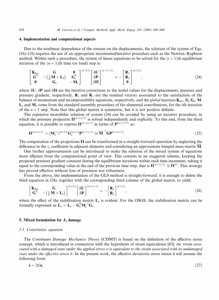
4. Implementation and computational aspects

Due to the nonlinear dependence of the stresses on the displacements, the solution of the system of Eqs.

(16)–(18) requires the use of an appropriate incremental/iterative procedure such as the Newton–Raphson

method. Within such a procedure, the system of linear equations to be solved for the ðiþ 1Þth equilibrium

iteration of the ðnþ 1Þth time (or load) step is:

Kdev G 0

GT � 1K Mþ Ls

� �GT

s

0 Gs �Ms

24 35ðnþ1;iÞdUdPdP

24 35ðnþ1;iþ1Þ

¼ �R1

R2

0

24 35ðnþ1;iÞ

; ð24Þ

where dU, dP and dP are the iterative corrections to the nodal values for the displacements, pressure andpressure gradient, respectively, R1 and R2 are the residual vectors associated to the satisfaction of the

balance of momentum and incompressibility equations, respectively, and the globalmatrices Kdev, G, Gs,M,

Ls and Ms come from the standard assembly procedure of the elemental contributions, for the ith iteration

of the nþ 1 step. Note that this global matrix is symmetric, but it is not positive definite.

The expensive monolithic solution of system (24) can be avoided by using an iterative procedure, in

which the pressure projection Pðnþ1;iþ1Þ is solved independently and explicitly. To this end, from the third

equation, it is possible to express Pðnþ1;iþ1Þ in terms of Pðnþ1;iþ1Þ as:

Pðnþ1;iþ1Þ ¼ ðM�1s Þðnþ1;iÞ

Gðnþ1;iÞs Pðnþ1;iþ1Þ ffi M

�1GPðnþ1;iþ1Þ: ð25Þ

The computation of the projections P can be transformed in a straight-forward operation by neglecting the

difference in the se coefficient in adjacent elements and considering an approximate lumped mass matrix M.

One further approximation can be introduced to make the solution of the mixed system of equations

more efficient from the computational point of view. This consists in an staggered scheme, keeping theprojected pressure gradient constant during the equilibrium iterations within each time increment, taking it

equal to the corresponding value at the end of the previous time step, that is Pðnþ1;iþ1Þ ffi PðnÞ. This strategy

has proved effective without loss of precision nor robustness.

From the above, the implementation of the GLS method is straight-forward; it is enough to delete the

third equation in (24), together with the corresponding third column of the global matrix, to yield:

Kdev GGT � 1

K Mþ Ls

� �� ðnþ1;iÞdUdP

� � nþ1;iþ1ð Þ

¼ � R1

R2

� �ðnþ1;iÞ

; ð26Þ

where the effect of the stabilization matrix Ls is evident. For the OSGS, the stabilization matrix can be

formally expressed as bLs ¼ Ls �GTsM

�1s Gs.

5. Mixed formulation for J2 damage

5.1. Constitutive equation

The Continuum Damage Mechanics Theory (CDMT) is based on the definition of the effective stress

concept, which is introduced in connection with the hypothesis of strain equivalence [43]: the strain asso-

ciated with a damaged state under the applied stress r is equivalent to the strain associated with its undamaged

state under the effective stress �r. In the present work, the effective deviatoric stress tensor �s will assume the

following form:

�s ¼ 2Ge: ð27Þ


The constitutive equation for the J2-damage model is defined as:

p ¼ Kev; ð28Þ

s ¼ ð1� dÞ�s ¼ ð1� dÞ2Ge; ð29Þwhere we have introduced one internal-like variable, d, the damage index, whose definition and evolutionis given below.

5.2. Characterization of damage

In order to clearly define concepts such as loading, unloading, or reloading for general 3D stress states, a

scalar positive quantity, termed as equivalent stress, is defined. This allows the comparison of different 2D

and 3D stress states. With such a definition, distinct 3D stress states can be mapped to a single equivalent

1D shear test, which makes their quantitative comparison possible [44,45].In the present work, the equivalent stress will assume the following form:

s ¼ffiffi32

qk�sk ¼

ffiffi32

q½�s : �s�1=2; ð30Þ

which corresponds to the usual definition of the equivalent von Mises stress �s.With the above definition for the equivalent effective stress, the damage criterion, U, is introduced as:

Uðs; rÞ ¼ s� r ¼ �s� r6 0: ð31ÞVariable r is an internal stress-like variable that is interpreted as the current damage threshold, in the sense

that its value controls the size of the (monotonically) expanding damage surface. The initial value of thedamage threshold is r0 ¼ r0, where r0 is the initial uniaxial damage stress.

Note that the damage criterion is defined in the effective deviatoric stress space (or, alternatively, in the

deviatoric strain space). In the principal stress space, the shape of the damage criterion is defined by the

well-known von Mises cylinder with axis along the hydrostatic axis. Fig. 4a shows a schematic represen-

tation of this damage criterion.

The expansion of the damage bounding surface in the normalized space for loading, unloading and

reloading conditions is controlled by the Kuhn–Tucker relations and the damage consistency condition,

which are

_rP 0; Uðs; rÞ6 0; _rUðs; rÞ ¼ 0; ð32aÞ

Fig. 4. J2-damage model: (a) damage surface and (b) softening functions.


If Uðs; rÞ ¼ 0 then _r _Uðs; rÞ ¼ 0 ð32bÞ

leading, in view of Eq. (31), to the loading condition

_r ¼ _s: ð33Þ

This, in turn, leads to the explicit definition of the current values of the internal variable r in the form

r ¼ maxfr0;maxðsÞg: ð34ÞNote that Eq. (34) allows to compute the current values for r in terms of the current value of s, whichdepends explicitly on the current deviatoric strains (see Eqs. (62) and (30)).

Finally, the damage index d ¼ dðrÞ is explicitly defined in terms of the corresponding current value of the

damage threshold, so that it is a monotonically increasing function such that 06 d 6 1.

In this work, we will use the following functions:

• Linear softening:

dðrÞ ¼ ð1þ HSÞ 1� r0r

� ; r0 6 r6 ru ¼ r0 1þ 1

HS

� �;

1; ru P r:

8<: ð35Þ

• Exponential softening:

dðrÞ ¼ 1� r0rexp

� 2HS

r � r0r0

� ��; r0 6 r: ð36Þ

where HS P 0 is a constant.

It is also possible to express the damage laws in the form [46]:

dðrÞ ¼ 1� qðrÞr

r0 6 r; ð37Þ

where the function q ¼ qðrÞ ¼ ð1� dðrÞÞr is the stress-like softening function.

In this format, the softening laws can be rewritten as

• Linear softening:

qðrÞ ¼ r0 � HSðr � r0Þ; r0 6 r6 ru;1; ru P r:

ð38Þ

• Exponential softening:

qðrÞ ¼ r0 exp� 2HS

r � r0r0

� ��; r0 6 r: ð39Þ

Fig. 4b shows a schematic representation of both these functions.

5.3. Rate dependent damage

In many materials there is a strong coupling between nonlinear rate-sensitivity and damage growth.

Therefore, it is natural to develop a rate dependent constitutive model within the framework of CDMT,


evolving from the above presented rate independent damage model, and which accounts for strain ratedependency via the damage evolution laws [37].

To this end, let us consider a viscous regularization of the rate-independent damage threshold evolution

law defined by Eq. (33), so that this is replaced by:

_r ¼ hs� ri#

; ð40Þ

where h�i are the Macaulay brackets and # is the retardation time for damage.Note that this modification of the evolution law only affects the integration of the damage threshold r,

but not the damage variable d itself. This is still obtained in a closed form, through the explicit definition of

the function d ¼ dðrÞ. Additionally, it is worth to remark that Eq. (40) guarantees monotonic increasing of

the damage threshold, and, therefore, also of the damage index ( _dP 0).

It must be noted that the definition of the evolution law (40) replaces the Kuhn–Tucker and consistency

conditions, Eqs. (32a) and (32b), of the rate independent model.

The reasoning behind the above law is analogous to the classical Perzyna viscoplastic regularization

often used in the framework of Computational Plasticity. It can be seen that this assumed rate dependentformulation is a general form for the evolution of the damage threshold, so that for a null value of the

retardation damage parameter, the rate-independent (or inviscid) damage evolution law is recovered ex-

actly, while for an infinite value of #, evolution of the damage variables is prevented, thus rendering an

instantaneously elastic response.

The rate-dependent model can also be written in a Duvaut–Lions format, as

_r ¼ hr1 � ri#

P 0; ð41Þ

where r1 is the value of the damage threshold corresponding to the current value of s as t=# ! 1. As the

rate-dependent (viscous) model relaxes to the rate-independent (inviscid) solution, it is obvious that in the

inviscid limit, satisfaction of the consistency condition ensures that r1 ¼ s. Therefore, Eqs. (40) and (41)

are completely equivalent.

5.4. Thermodynamic framework

Let us define the elastic free energy in the form

W e ¼ WvolðevÞ þ W edevðeÞ; ð42Þ

¼ 12Ke2v þ 1

2ð2GÞe : eP 0: ð43Þ

The mechanical free energy term for the damage model is defined in the form:

W ¼ WvolðevÞ þ ð1� dÞW edevðeÞ; ð44Þ

¼ 12Ke2v þ ð1� dÞ1

2ð2GÞe : eP 0: ð45Þ

From this, and recalling that 06 d 6 1, it is obvious that W P 0.

The constitutive equation for the damage model is obtained using Coleman�s method as:

p ¼ oevW ¼ Kev; ð46Þ

s ¼ oeW ¼ ð1� dÞ2Ge: ð47ÞThe mechanical dissipation can be expressed as

_D ¼ W edev

_dP 0 ð48Þprovided that the damage index increases monotonically, _dP 0.


5.5. Softening behaviour and regularization

Expressions (35) and (36) are able to reproduce the softening branch that occurs in a 1D shear test after

the peak stress is reached, with the shear stress decreasing asymptotically to the strain axis. With these

evolution laws for d, a finite area is retained between the stress-strain curve and the strain axis. This area

defines the available energy to be dissipated in the control volume.

In finite element analysis this entails the loss of objectivity of the results, in the sense that the inelastic

shear strains tend to localize in a band that is only one element across, independently of the element size he.Upon mesh refinement, as he tends to zero, strains tend to concentrate on a band of zero thickness (a

geometrical line), and no energy is dissipated in the failure process. Clearly, this is physically unacceptable.

In order to remedy this well-accounted for fact, Ref. [47] proposed the use of the so-called ‘‘fracture

energy regularization technique’’, nowadays used in many FE applications. This strategy is followed in this

work, as it is extremely convenient from the computational standpoint, while guaranteeing the correct

conservation of dissipated energy upon mesh refinement.

It has to be remarked that this technique constitutes a crucial and appealing ‘‘lost-link’’ between

Continuum and Fracture Mechanics, two disciplines that have often been presented as wide apart ways ofapproaching Failure Mechanics.

The fracture energy regularization technique is based on the assumption that dissipation takes place in a

band only one element thick, irrespective of the element size. The basic concept consists on modifying the

softening law in such a way that the energy dissipated over a completely degraded finite element be equal to

a given value, which depends on the fracture energy of the material and on the element size. For each

element, the material characteristic length [48,49] is approximated by the element characteristic length lch[50], which depends on the geometric dimensions of the element and measures the computational width of

the fracture zone. The specific dissipated energy D is then scaled for each element so that the equation

Dlch ¼ GII ð49Þholds, where GII is the mode II fracture energy of the material, regarded to be a material property. As it is

shown below, this makes the softening modulus HS, which defines the softening response, dependent on the

element size. It also sets a maximum size for the elements that can be used in the analysis. The procedure is

as follows.

5.5.1. Rate independent behaviour

Consider an ideal experiment in which the load increases monotonically and quasi-statically from an

initial unstressed state to another in which full degradation takes place.

Using the rate independent version of the damage model, the specific energy dissipated in the process is:

D ¼Z t¼1

t¼0

_Ddt ð50Þ

¼Z t¼1

t¼0

W edev

_d dt ð51Þ

¼ 2=3

2ð2GÞ

Z r¼1

r¼r0

r2d 0 dr; ð52Þ

where we have used Eqs. (30), (34), (44), (48) and (62) and the rate of damage can be expressed as _d ¼ d 0 _r.We will consider in the following both the cases of linear and exponential softening:

• Linear softening: Using Eq. (35), d 0 ¼ ð1þ HSÞr0=r2, for r0 6 r6 ru, with ru ¼ r0ð1þ 1=HSÞ, and d 0 ¼ 0,otherwise. Recalling that r0 ¼ r0, integrating and equating D ¼ GII=lch, we have


D ¼ 1

�þ 1

HS

�r20

3ð2GÞ ¼GII

lchð53Þ

and, therefore,

HS ¼HSlch

1� HSlchP 0; ð54Þ

where HS ¼ r20=ð3ð2GÞGIIÞ depends on the material properties, as GII is the mode II fracture energy per

unit area, r0 is the uniaxial strength and G is the shear modulus.

• Exponential softening: Using now Eq. (36), d 0 ¼ ðr0 þ 2HSrÞ expf�2HSðr�r0r0Þg=r2, for r0 6 r61. Recall-

ing that r0 ¼ r0, and integrating, we have

D ¼ 1

�þ 1

HS

�r20

3ð2GÞ ; ð55Þ

which is identical to the result in (53).

In the framework of local models and finite element analysis, the state variables are computed at the

integration points in terms of the local strain (and/or stress) history. Therefore, the threshold and damage

internal variables are defined at the integration points. The characteristic length is thus related to the

volume (or area) of each finite element.For linear simplicial elements, the characteristic length can be taken as the representative size of the

element, lch ¼ he. In this work, and assuming that the elements are equilateral, the size of the element will be

computed as h2e ¼ ð4=ffiffiffi3

pÞAe for triangular elements, Ae being the area of the element, and as h3e ¼

ð12=ffiffiffi2

pÞVe for tetrahedral elements, where Ve is the volume of the element.

It is clear from Eq. (54) that the introduction of the characteristic length implies a limitation on the

maximum size of the finite elements used in the mesh, he 6 1=HS. The greater the elements, the steeper is the

softening branch of the response, and, locally, the fracture process is more brittle. For he > 1=HS the ratio

GII=he is smaller that the elastic energyW stored by the element, and a dynamic snap-back would occur at theonset of damage.

5.5.2. Rate dependent behaviour

Let us now consider an ideal experiment in which the load increases monotonically, and not quasi-

statically from an initial unstressed state to another in which full degradation takes place.

Using the rate dependent version of the model, the specific energy dissipated in the process is:

D ¼Z t¼1

t¼0

_Ddt ð56aÞ

¼Z t¼1

t¼0

W edev

_d dt ð56bÞ

¼ 2=3

2ð2GÞ

Z r¼1

r¼r0

½r þ #_r�2d 0 dr; ð56cÞ

where we have used Eqs. (40), (44), (48) and (62) and the rate of damage can be expressed as _d ¼ d 0 _r.Comparing Eq. (56c) with Eq. (52) it is obvious that the first one reduces to the second for a null value of

#, or for very slow processes, with _r tending to zero.

In other cases, the evolution law, Eq. (40), ensures that the terms r and #_r are of the same order, that is

ð#_r=rÞ ¼ Oð1Þ. Therefore, it can be assumed that the regularized parameter from Eq. (54), that regularizes the

rate independent model, will also regularize the rate dependent model, both for linear and exponential softening.


It must be remarked that formats of the regularized damage law different from that of Eq. (41) may leadto the necessity of regularizing also the damage retardation time #, making it dependent on the element size

[37,51].

5.6. Update of the damage threshold

A numerical algorithm needs to be implemented for the time integration of the damage constitutive

equations presented in the previous sections. In the following this algorithm is presented, in a strain-driven

form which leads to a completely closed-form algorithm to integrate the stress tensor in time. This is mostappropriate within the context of the application of the finite element method.

Each time step begins at time tn with all state variables known and it ends at time tnþ1 with the state

variables updated according to the given total strain tensor enþ1. The time step size is Dt ¼ tnþ1 � tn.For the rate independent model, Eq. (34) allows to compute the current value for rnþ1 in terms of the

current value of snþ1, which in turn, depends explicitly on the current strains enþ1 (see Eqs. (62) and (30)).

After this, the damage index dnþ1 ¼ dnþ1ðrnþ1Þ is explicitly computed in terms of the corresponding current

value of the damage threshold, using the appropriate expression, Eq. (35) or (36).

For the rate dependent model, the only difference is the updating of the damage threshold rnþ1 whenevolution of the damage occurs, that is, upon loading conditions. This may be evaluated using a generalized

mid-point rule to integrate Eq. (40), i.e.,

rnþ1 ¼ rn þ Drnþ1 ¼ rn þDt#hsa � rai; ð57Þ

where sa and ra are defined by:

sa ¼ ð1� aÞsn þ asnþ1; ð58aÞ

ra ¼ ð1� aÞrn þ arnþ1: ð58bÞ

The choice a ¼ 1 Eq. (57) corresponds to a backward-Euler difference scheme. It is easy to show that the

algorithm of Eq. (57) is unconditionally stable for aP 0:5 and second order accurate only for a ¼ 0:5(Crank–Nicholson or trapezoidal rule), which allows the use of larger time step sizes for rate-dependent

analysis.

Substituting Eqs. (58a) and (58b) into Eq. (57), yields

rnþ1 ¼ max rn;1

1þ a Dt#

1

��(� ð1� aÞDt

#

�rn þ

Dt#sa

�): ð59Þ

It is worth to remark that the presented method for the integration of the damage threshold is also valid for

the rate independent model, noting that for # ¼ 0 and a ¼ 1, Eq. (59) simply reduces to the satisfaction of

the monotonicity and consistency conditions

rnþ1 ¼ maxfrn; snþ1g: ð60Þ

5.7. Tangent operator

5.7.1. Rate independent damage

Differentiating Eq. (29) with respect to time, we obtain

_s ¼ ð1� dÞ_�s� _d�s: ð61Þ


The effective deviatoric stresses �s can be computed in terms of the total strain tensor e as

�s ¼ Cdev : e; ð62Þ

where Cdev ¼ 2G½I� 13ð1� 1Þ� is the usual (fourth order) linear–elastic deviatoric constitutive tensor, I is the

(fourth order) unit tensor and (:) denotes the tensor product contracted on two indices. Differentiating this

with respect to time, we have

_�s ¼ Cdev : _e: ð63Þ

On the other hand, the time derivative of the damage index is

_d ¼ d 0 _r; ð64Þwhere the derivative d 0 ¼ d 0ðrÞ can be obtained from Eqs. (35) and (36). On loading, consistency requires

that _r ¼ _s, and therefore, differentiating Eq. (30), we can write

_r ¼ _s ¼ 1

s�s : _�s ¼ 3

2

2Gs�s : _e: ð65Þ

On unloading, it is _r ¼ 0. Substituting this result in Eq. (64), and the result in Eq. (61), yields the desired

expression

_s ¼ Ctandev : _e; ð66Þ

with

Ctandev ¼ ð1� dÞð2GÞ I

�� 1

3ð1� 1Þ

� hð�s� �sÞ; ð67Þ

where I is the (fourth order) unit tensor, 1 is the (second order) unit tensor and the scalar coefficient h is

h ¼3

2

2Gsd 0 for loading;

0 for unloading:

8<: ð68Þ

The complete constitutive tensor includes the volumetric part:

Ctan ¼ Kð1� 1Þ þ ð1� dÞð2GÞ I

�� 1

3ð1� 1Þ

�� hð�s� �sÞ; ð69Þ

which defines the rate constitutive equation

_r ¼ Ctan : _e: ð70Þ

5.7.2. Rate dependent damage

In the case of rate dependent damage the determination of _r comes from differentiating Eq. (57) with

respect to time, to yield:

_r ¼aDt#

1þ aDt#

_s: ð71Þ

Comparing Eqs. (65) and (71), it is obvious that the tangent operator for the rate dependent damage case

has the same expression of Eq. (67) with the coefficient h given by


h ¼aDt#

1þ aDt#

3

2

2Gsd 0 for loading;

0 for unloading:

8>>><>>>: ð72Þ

Note that for large values of Dt=# the rate independent case is recovered.

5.8. Stabilization parameter

The stabilization techniques discussed in the previous section are designed to provide global stability to

the incompressible elasto-damage problem. For the J2-damage model proposed above, the definition of the

stabilization parameter is straight-forward, as the secant (damaged) shear modulus is simply G� ¼ð1� dÞG:

se ¼ch2e2G� ¼

ch2eð1� dÞ2G : ð73Þ

6. Numerical examples

The formulation presented in the preceding sections is illustrated below in a number of benchmark

problems. Performance of the standard irreductible, the standard mixed and the proposed mixed formu-

lations are tested considering 2D plane-strain 3-noded linear triangular meshes. The examples involve

compressible elasticity and isotropic J2-damage with exponential softening.

The following material properties are assumed: Young�s modulus E ¼ 10 MPa, Poisson�s ratio m ¼ 0:3(recall that G ¼ E=2ð1þ mÞ, K ¼ E=3ð1� 2mÞ), uniaxial damage stress r0 ¼ 10 kPa and mode II fracture

energy GII ¼ 200 J/m2. A value c ¼ 1 is taken for the evaluation of se. A value c0 ¼ 10 is used for theevaluation of the viscous regularization.

The Newton–Raphson method, combined with a line search procedure, is used to solve the non-linear

system of equations arising from the spatial and temporal discretization of the weak form of the stabilized

problem. In all cases 200 equal time steps are performed to complete the analyses.

Convergence of a step is attained when the ratio between the iterative and the incremental norm of the

computed displacements is lower than 0.01 (1%). Calculations are performed with an enhanced version of

the finite element program COMET [52], developed by the authors at the International Center for

Numerical Methods in Engineering (CIMNE). Pre and post-processing is done with GiD, also developed atCIMNE [53].

6.1. Singly perforated strip

The first example is a plane-strain singly perforated strip subjected to axial imposed straining. Because of

the double symmetry of the domain and boundary conditions, only one quarter of the domain (the top right

quarter) needs to be discretized. Fig. 5a depicts the original geometry of the problem; dimensions are

20 · 40 m ·m (width ·height) and the radius of the perforation is r ¼ 1 m. Thickness is 1 m.The computational domain is divided into an unstructured uniform mesh of 7336 linear triangles (3801

nodes) with an average mesh size of he ¼ 0:25 m, not shown. The pre-processor used tends to introduce

patches of equilateral triangles with predominant directions at )30�, +30� and +90� with the horizontal

axis.

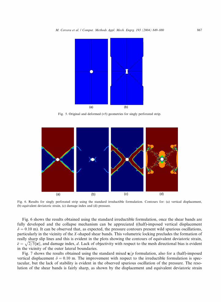
Fig. 5. Original and deformed (·5) geometries for singly perforated strip.

Fig. 6. Results for singly perforated strip using the standard irreductible formulation. Contours for: (a) vertical displacement,

(b) equivalent deviatoric strain, (c) damage index and (d) pressure.


Fig. 6 shows the results obtained using the standard irreductible formulation, once the shear bands arefully developed and the collapse mechanism can be appreciated ((half)-imposed vertical displacement

d ¼ 0:10 m). It can be observed that, as expected, the pressure contours present wild spurious oscillations,

particularly in the vicinity of the X -shaped shear bands. This volumetric locking precludes the formation of

really sharp slip lines and this is evident in the plots showing the contours of equivalent deviatoric strain,�e ¼

ffiffiffiffiffiffiffiffi2=3

pkek, and damage index, d. Lack of objectivity with respect to the mesh directional bias is evident

in the vicinity of the outer lateral boundaries.

Fig. 7 shows the results obtained using the standard mixed u=p formulation, also for a (half)-imposed

vertical displacement d ¼ 0:10 m. The improvement with respect to the irreductible formulation is spec-tacular, but the lack of stability is evident in the observed spurious oscillation of the pressure. The reso-

lution of the shear bands is fairly sharp, as shown by the displacement and equivalent deviatoric strain

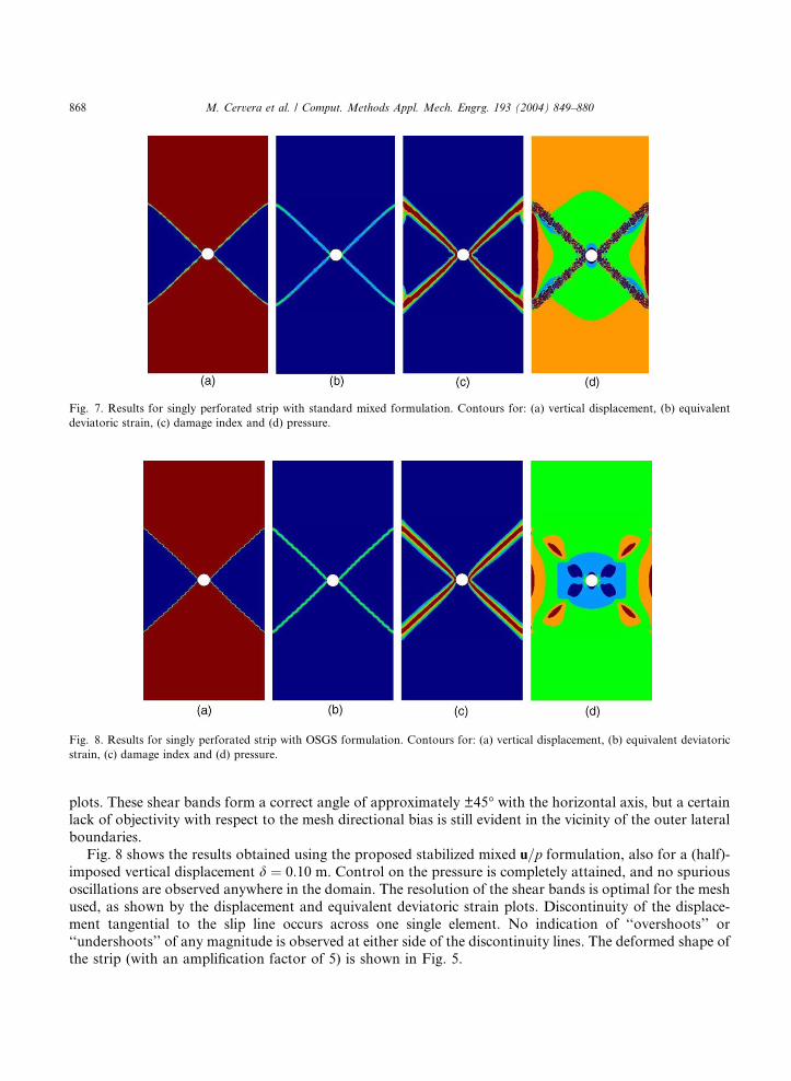
Fig. 7. Results for singly perforated strip with standard mixed formulation. Contours for: (a) vertical displacement, (b) equivalent

deviatoric strain, (c) damage index and (d) pressure.

Fig. 8. Results for singly perforated strip with OSGS formulation. Contours for: (a) vertical displacement, (b) equivalent deviatoric

strain, (c) damage index and (d) pressure.


plots. These shear bands form a correct angle of approximately ±45� with the horizontal axis, but a certainlack of objectivity with respect to the mesh directional bias is still evident in the vicinity of the outer lateral

boundaries.

Fig. 8 shows the results obtained using the proposed stabilized mixed u=p formulation, also for a (half)-

imposed vertical displacement d ¼ 0:10 m. Control on the pressure is completely attained, and no spurious

oscillations are observed anywhere in the domain. The resolution of the shear bands is optimal for the mesh

used, as shown by the displacement and equivalent deviatoric strain plots. Discontinuity of the displace-

ment tangential to the slip line occurs across one single element. No indication of ‘‘overshoots’’ or

‘‘undershoots’’ of any magnitude is observed at either side of the discontinuity lines. The deformed shape ofthe strip (with an amplification factor of 5) is shown in Fig. 5.


Fig. 9 shows the evolution of the damage index at four different stages of the analysis, for: (a) d ¼ 0:010m, (b) d ¼ 0:015 m, (c) d ¼ 0:020 m and (d) d ¼ 0:025 m. Note that the localization bands form completely

at a very early stage of the analysis, and in a quite ‘‘explosive’’ fashion. The damage index of the elements

inside the localization bands reaches values very close to unity, complete shear degradation, very early

during the analysis.

Fig. 10 shows (half)-load vs (half)-imposed vertical displacement curves (recall 1 m thickness is assumed)

obtained with the three formulations: (a) standard irreductible, (b) standard mixed and (c) mixed with

OSGS stabilization. Two remarks are in order. First, both the mixed formulations capture reasonably well

both the limit load and the general softening trend of the curve, while the irreductible formulation fails todo so almost completely. Second, the effect of the stabilization techniques adopted is obvious in the global

Fig. 9. Evolution of damage for singly perforated strip. Contours for (half)-imposed vertical displacement equal to: (a) 0.010, (b)

0.015, (c) 0.020 and (d) 0.025.

0

20

40

60

80

100

0 0.02 0.04 0.06 0.08 0.1

DISPLACEMENT-Y [m]

OSGS Stabilization Standard Mixed Up

Standard Irreductible

1/2

RE

AC

TIO

N-Y

[kN

]

Fig. 10. Load versus displacement for simply perforated strip. Comparison among different formulations.


softening response, with clear advantage for the proposed OSGS method. As it has been explained, thedifferences in the responses are due to the different degrees of success of the formulations in removing the

volumetric locking induced by the isochoric deformational behaviour inside the shear bands.

Finally, Fig. 11 shows (half)-load vs (half)-imposed vertical displacement curves (1 m thickness is as-

sumed) obtained with two uniform unstructured meshes with two element sizes: (a) he ¼ 0:25 m and (b)

he ¼ 0:50 m (1820 elements, 977 nodes). Note that the overall global response is satisfactorily similar upon

mesh refinement, with the total area under the load–displacement curve converging to the correct amount

of mechanical dissipation dissipated to create the localization bands. No spurious brittleness is observed

when the size of the elements is reduced. This is achieved by the regularization procedure explained inSection 5.5.

6.2. Doubly perforated strip

The second example is a plane-strain doubly perforated strip subjected to axial imposed straining. Be-

cause of the double symmetry of the domain and boundary conditions, only one quarter of the domain (the

top right quarter) is discretized. Fig. 12a depicts the original geometry of the problem; dimensions are

20 · 40 m ·m (width ·height) and the radius of the perforations is r ¼ 1 m. Thickness is 1 m.This example is interesting because, as it will be shown below, the symmetric collapse mechanism

consists of multiple shear bands that intersect each other. Therefore, it is an adequate test to assess the

ability of the different formulations to deal with such a complex situation.

The computational domain is divided into an unstructured uniform mesh of 7289 linear triangles (3780

nodes) with an average mesh size of he ¼ 0:25 m.

Fig. 13 shows the results obtained using the standard irreductible formulation, once the shear bands are

fully developed and the collapse mechanism can be appreciated ((half)-imposed vertical displacement

d ¼ 0:10 m). As expected, the pressure contours present wild spurious oscillations, particularly in thevicinity of the double X -shaped shear bands. This volumetric locking precludes the formation of really

sharp slip lines and this is evident in the plots showing the contours of equivalent deviatoric strain and

0

20

40

60

80

100

0 0.02 0.04 0.06 0.08 0.1Half DISPLACEMENT-Y [m]

h = 0.25 h = 0.50

Hal

f R

EA

CT

ION

-Y [

kN]

Fig. 11. Load versus displacement for simply perforated strip. Comparison between different mesh sizes.

Fig. 13. Results for doubly perforated strip using the standard irreductible formulation. Contours for: (a) vertical displacement, (b)

equivalent deviatoric strain, (c) damage index and (d) pressure.

Fig. 12. Original and deformed (·5) geometries for doubly perforated strip.


damage index. Lack of objectivity with respect to the mesh directional bias is evident, as the shear bands

form an incorrect angle of ±30� with the horizontal axis.

Fig. 14 shows the results obtained using the standard mixed u=p formulation, also for a (half)-imposed

vertical displacement d ¼ 0:10 m. The improvement with respect to the irreductible formulation is

remarkable, as the shear bands form a correct angle of approximately ±45� with the horizontal axis, but a

certain lack of objectivity with respect to the mesh directional bias is evident in the vicinity of the outer

lateral boundaries, where some of the slip lines bifurcate. The lack of stability of the formulation is evidentin the observed spurious oscillation of the pressure. The resolution of the shear bands is fairly sharp, as

shown by the displacement and equivalent deviatoric strain plots.

Fig. 14. Results for doubly perforated strip with standard mixed formulation. Contours for: (a) vertical displacement, (b) equivalent


Fig. 15. Results for doubly perforated strip with OSGS formulation. Contours for: (a) vertical displacement, (b) equivalent deviatoric



Fig. 15 shows the results obtained using the proposed stabilized mixed u=p formulation, also for a

(half)-imposed vertical displacement of d ¼ 0:10 m. Full control on the pressure is attained, and no

spurious oscillations are observed anywhere. The resolution of the shear bands is optimal, as shown by

the displacement and the equivalent deviatoric strain contour plots, where the discontinuities occur

across one single element. No spurious branching of the slip lines occurs near the lateral boundaries. The

deformed shape of the perforated strip (with a displacement amplification factor of 5) is shown in Fig.

12b.Fig. 16 shows the evolution of the damage index at four different stages of the analysis, for: (a) d ¼ 0:010

m, (b) d ¼ 0:020 m, (c) d ¼ 0:030 m and (d) d ¼ 0:040 m. Also in this example the localization bands form

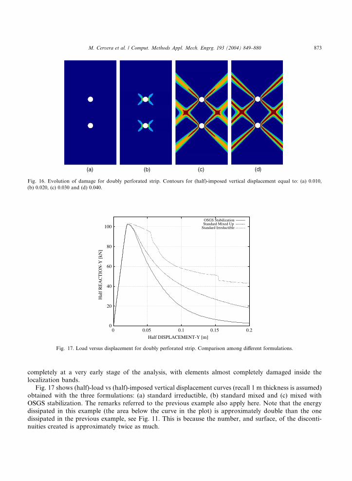
Fig. 16. Evolution of damage for doubly perforated strip. Contours for (half)-imposed vertical displacement equal to: (a) 0.010,

(b) 0.020, (c) 0.030 and (d) 0.040.

0

20

40

60

80

100

0 0.05 0.1 0.15 0.2

Half DISPLACEMENT-Y [m]



Hal

f R

EA

CT

ION

-Y [

kN]

Fig. 17. Load versus displacement for doubly perforated strip. Comparison among different formulations.


completely at a very early stage of the analysis, with elements almost completely damaged inside the

localization bands.



OSGS stabilization. The remarks referred to the previous example also apply here. Note that the energy

dissipated in this example (the area below the curve in the plot) is approximately double than the one

dissipated in the previous example, see Fig. 11. This is because the number, and surface, of the disconti-

nuities created is approximately twice as much.


Finally, Fig. 18 shows (half)-load vs (half)-imposed vertical displacement curves (1 m thickness is as-sumed) obtained with two uniform unstructured meshes with two element sizes: (a) he ¼ 0:25 m and (b)

he ¼ 0:50 m (1794 elements, 965 nodes). No spurious brittleness is observed when the size of the elements is

reduced.

6.3. Multiply perforated strip

The last example is a plane-strain strip with four circular perforations subjected to axial imposed

straining. Because of the double symmetry of the domain and boundary conditions, only one quarter of thedomain (the top right quarter) is discretized. Fig. 19a depicts the original geometry of the problem; as in the

0

20

40

60

80

100

0 0.05 0.1 0.15 0.2

Hal

f R

EA

CT

ION

-Y [

kN]


h = 0.25 h = 0.50

Fig. 18. Load versus displacement for doubly perforated strip. Comparison between different mesh sizes.

Fig. 19. Original and deformed (·5) geometries for multiply perforated strip.


previous examples, dimensions are 20 · 40 m ·m (width · height) and the radius of the perforations is r ¼ 1m. Thickness is 1 m.

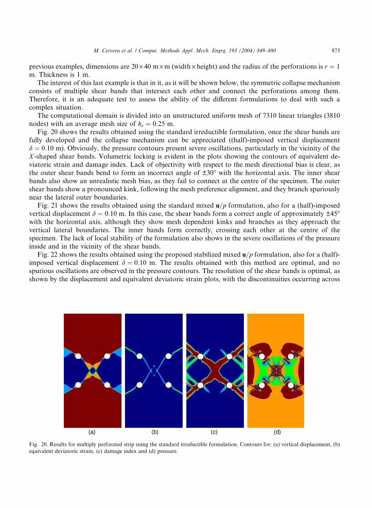
The interest of this last example is that in it, as it will be shown below, the symmetric collapse mechanism

consists of multiple shear bands that intersect each other and connect the perforations among them.

Therefore, it is an adequate test to assess the ability of the different formulations to deal with such a

complex situation.

The computational domain is divided into an unstructured uniform mesh of 7310 linear triangles (3810

nodes) with an average mesh size of he ¼ 0:25 m.

Fig. 20 shows the results obtained using the standard irreductible formulation, once the shear bands arefully developed and the collapse mechanism can be appreciated ((half)-imposed vertical displacement

d ¼ 0:10 m). Obviously, the pressure contours present severe oscillations, particularly in the vicinity of the

X -shaped shear bands. Volumetric locking is evident in the plots showing the contours of equivalent de-

viatoric strain and damage index. Lack of objectivity with respect to the mesh directional bias is clear, as

the outer shear bands bend to form an incorrect angle of ±30� with the horizontal axis. The inner shear

bands also show an unrealistic mesh bias, as they fail to connect at the centre of the specimen. The outer

shear bands show a pronounced kink, following the mesh preference alignment, and they branch spuriously

near the lateral outer boundaries.Fig. 21 shows the results obtained using the standard mixed u=p formulation, also for a (half)-imposed

vertical displacement d ¼ 0:10 m. In this case, the shear bands form a correct angle of approximately ±45�with the horizontal axis, although they show mesh dependent kinks and branches as they approach the

vertical lateral boundaries. The inner bands form correctly, crossing each other at the centre of the

specimen. The lack of local stability of the formulation also shows in the severe oscillations of the pressure

inside and in the vicinity of the shear bands.

Fig. 22 shows the results obtained using the proposed stabilized mixed u=p formulation, also for a (half)-

imposed vertical displacement d ¼ 0:10 m. The results obtained with this method are optimal, and nospurious oscillations are observed in the pressure contours. The resolution of the shear bands is optimal, as

shown by the displacement and equivalent deviatoric strain plots, with the discontinuities occurring across

Fig. 20. Results for multiply perforated strip using the standard irreductible formulation. Contours for: (a) vertical displacement, (b)

equivalent deviatoric strain, (c) damage index and (d) pressure.

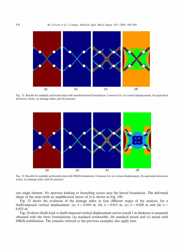
Fig. 21. Results for multiply perforated strip with standard mixed formulation. Contours for: (a) vertical displacement, (b) equivalent


Fig. 22. Results for multiply perforated strip with OSGS formulation. Contours for: (a) vertical displacement, (b) equivalent deviatoric



one single element. No spurious kinking or branching occurs near the lateral boundaries. The deformedshape of the strip (with an amplification factor of 5) is shown in Fig. 19b.

Fig. 23 shows the evolution of the damage index at four different stages of the analysis, for a

(half)-imposed vertical displacement: (a) d ¼ 0:010 m, (b) d ¼ 0:015 m, (c) d ¼ 0:020 m and (d) d ¼0:025 m.



OSGS stabilization. The remarks referred to the previous examples also apply here.

Fig. 23. Evolution of damage for multiply perforated strip. Contours for (half)-imposed vertical displacement equal to: (a) 0.010, (b)

0.015, (c) 0.020 and (d) 0.025.

0

20

40

60

80

100

0 0.02 0.04 0.06 0.08 0.1

Hal

f R

EA

CT

ION

-Y [

kN]




Fig. 24. Load versus displacement for multiply perforated strip. Comparison among different formulations.


Finally, Fig. 25 shows (half)-load vs (half)-imposed vertical displacement curves (1 m thickness is as-sumed) obtained with two uniform unstructured meshes with two element sizes: (a) he ¼ 0:25 m and (b)

he ¼ 0:50 m (1810 elements, 977 nodes). Once again, no spurious brittleness is observed when the size of the

elements is reduced.

0

20

40

60

80

100

0 0.02 0.04 0.06 0.08 0.1

Hal

f R

EA

CT

ION

-Y [

kN]


h = 0.25 h = 0.50

Fig. 25. Load versus displacement for multiply perforated strip. Comparison between different mesh sizes.


7. Conclusions

This paper shows the application of stabilized mixed linear simplex (triangles and tetrahedra) to thesolution of shear band localization problems via a local isotropic continuum J2 damage model.

A fully stable formulation of the problem is obtained using the orthogonal sub-grid scales (OSGS)

approach, which allows equal order interpolation of the displacement and pressure fields. This translates in

the achievement of three crucial goals:

• (a) The solution of the corresponding localization boundary value problem exists and it is unique.

• (b) The position and orientation of the localization bands is independent of the directional bias of the

finite element mesh.• (c) The global post-peak load–deflection curves are independent of the size of the elements in the local-

ization band.

The accomplishment of these fundamental objectives is attained by ensuring both global and local stability

of the problem.

A consistent residual viscous regularization is proposed and successfully applied, in order to over-

come the convergence difficulties often encountered in applications involving softening behaviour and

strain localization. The derived method yields a robust scheme, suitable for engineering applications in2D and 3D. The proposed formulation is shown to attain total control on the pressure field, removing

global and local oscillations induced by the incompressibility constraints induced by the material

model.

Numerical examples show, on one hand, the tremendous advantage of the mixed formulation over the

irreductible one to predict correct failure mechanisms with localized patterns of shear deformation, vir-

tually free from any dependence of the mesh directional bias; on the other, stabilization techniques are

shown to fully avoid the volumetric locking exhibited by the standard non-stable formulations, yielding a

correct global response in the softening regime.


Acknowledgements

The authors gratefully acknowledge the invaluable help of our colleagues Prof. R. Codina and Prof. S.

Oller, expressed in the form of unfailing suggestions and discussions.

References

[1] E.C. Aifantis, On the microstructural origin of certain inelastic models, Trans. ASME J. Engrg. Mater. Technol. 106 (1984) 326–

330.

[2] H. Schereyer, Z. Chen, One dimensional softening with localization, J. Appl. Mech., ASME 53 (1986) 791–797.

[3] I. Vardoulakis, E.C. Aifantis, A gradient flow theory of plasticity for granular materials, Acta Mech. 87 (1991) 197–217.

[4] R. de Borst, H.B. Mulhaus, Gradient-dependent plasticity: formulation and algorithm aspect, Int. J. Numer. Methods Engrg. 35

(1992) 521–539.

[5] J. Pamin, Gradient-Dependent Plasticity in Numerical Simulation of Localization Phenomena. Ph.D. Thesis, TU delft, The

Netherlands, 1994.

[6] R.H.J. Peerlings, R. de Borst, W.A.M. Brekelmans, M.G.D. Geers, Gradient-enhanced damage modelling of concrete failures,

Mech. Cohesive-Frict. Mater. 4 (1998) 339–359.

[7] M. Jir�asek, Nonlocal models for damage and fracture: comparison of approaches, Int. J. Solids Struct. 35 (1998) 4133–4145.

[8] R. de Borst, Some recent issues in computational failure mechanics, Int. J. Numer. Methods Engrg. 52 (2001) 63–95.

[9] R. de Borst, Simulation of strain localization: a repraisal of the Cosserat continuum, Engrg. Comput. 8 (1991) 317–322.

[10] P. Steinmann, K. Willam, Localization within the framework of micropolar elastoplasticy, in: V. Mannl et al. (Eds.), Advances in

Continuum Mechanics, Springer Verlag, Berlin, 1992, pp. 296–313.

[11] A. Needelman, Material rate dependence and mesh sensitivity in localization problems, Comput. Methods Appl. Mech. Engrg. 67

(1987) 68–75.

[12] J.C. Simo, J. Oliver, F. Armero, An analysis of strong discontinuities induced by strain-softening in rate-independent inelastic

solids, Comput. Mech. 12 (1993) 49–61.

[13] J. Oliver, Continuummodeling of strong discontinuities in solid mechanics using damage models, Comput. Mech. 17 (1995) 277–296.

[14] J. Oliver, M. Cervera, O. Manzoli, Strong discontinuities and continuum plasticity models: the strong discontinuity approach, Int.

J. Plasticity 15 (1999) 319–351.

[15] J. Oliver, A.E. Huespe, E. Samaniego, A study on finite elements for capturing strong discontinuities, Int. Numer. Methods Engrg.

56 (2003) 2135–2161.

[16] E.W.V. Chaves, A Three Dimensional Setting for Strong Discontinuities Modelling in Failure Mechanics, Ph.D. Thesis.

University of Catalonia, 2003.

[17] R. de Borst, Fracture in quasi-brittle materials: a review of continuum damage-based approaches, Engrg. Fract. Mech. 69 (2002)

95–112.

[18] O.C. Zienkiewicz, R.L. Taylor, The Finite Element Method, Butterworth-Heinemann, Oxford, 2000.

[19] O.C. Zienkiewicz, M. Pastor, M. Huang, Softening, localization and adaptive remeshing: capture of discontinuous solutions,

Comput. Mech. 17 (1995) 98–106.

[20] O.C. Zienkiewicz, M. Huang, M. Pastor, Localization problems in plasticity using finite elements with adaptive remeshing, Int. J.

Numer. Methods Geomech. 19 (1995) 127–148.

[21] J. Bonet, A.J. Burton, A simple average nodal pressure tetrahedral element for incompressible and nearly incompressible dynamic

explicit applications, Commun. Numer. Methods Engrg. 14 (1998) 437–449.

[22] O.C. Zienkiewicz, J. Rojek, R.L. Taylor, M. Pastor, Triangles and tetrahedra in explicit dynamic codes for solids, Int. J. Numer.

Methods Engrg. 43 (1998) 565–583.

[23] O. Klaas, A. Maniatty, M.S. Shephard, A stabilized mixed finite element method for finite elasticity. Formulation for linear

displacement and pressure interpolation, Comput. Methods Appl. Mech. Engrg. 180 (1999) 65–79.

[24] R.L. Taylor, A mixed formulation for triangular and tetrahedral elements, in: R. Abascal, J. Dom�ınguez, G. Bugeda, (Eds.),

Conference Proceedings on M�etodos Num�ericos en Ingenier�ıa, SEMNI, Barcelona, Spain, 1999.

[25] C.R. Dohrmann, M.W. Heinstein, J. Jung, S.W. Key, W.R. Witkowsky, Node-based uniform strain elements for three-node

triangular and four-node tetrahedral meshes, Int. J. Numer. Methods Engrg. 47 (2000) 1549–1568.

[26] R.L. Taylor, A mixed-enhanced formulation for tetrahedral elements, Int. J. Numer. Methods Engrg. 47 (2000) 205–227.

[27] J. Bonet, H. Marriot, O. Hassan, An averaged nodal deformation gradient linear tetrahedral element for large strain explicit

dynamic applications, Commun. Numer. Methods Engrg. 17 (2001) 551–561.

[28] J. Bonet, H. Marriot, O. Hassan, Stability and comparison of different linear tetrahedral formulations for nearly incompressible

explicit dynamic applications, Int. J. Numer. Methods Engrg. 50 (2001) 119–133.


[29] E. O~nate, J. Rojek, R.L. Taylor, O.C. Zienkiewicz, Linear triangles and tetrahedra for incompressible problem using a finite

calculus formulation, in: Proceedings of European Conference on Computational Mechanics, ECCM, 2001.

[30] E.A. de Souza Neto, F.M.A. Pires, D.R.J. Owen, A new F-bar-method for linear triangles and tetrahedra in the finite strain

analysis of nearly incompressible solids. in: Proceedings of VII International Conference on Computational Plasticity,

COMPLAS, 2003.

[31] M. Chiumenti, Q. Valverde, C. Agelet de Saracibar, M. Cervera, A stabilized formulation for incompressible elasticity using linear

displacement and pressure interpolations, Comput. Methods Appl. Mech. Engrg. 191 (2002) 5253–5264.

[32] M. Chiumenti, Q. Valverde, C. Agelet de Saracibar, M. Cervera, A stabilized formulation for incompressible plasticity using linear

triangles and tetrahedra, Int. J. Plasticity, in press.

[33] M. Cervera, M. Chiumenti, Q. Valverde, C. Agelet de Saracibar, Mixed linear/linear simplicial elements for incompressible

elasticity and plasticity, Comput. Methods Appl. Mech. Engrg. 192 (2003) 5249–5263.

[34] M. Cervera, Chiumenti, C. Agelet de Saracibar, Softening, localization and stabilization: capture of discontinuous solutions in J2plasticity, Int. J. Numer. Anal. Methods Geomech., submitted for publication.

[35] L.M. Kachanov, Time of rupture process under creep conditions, Izvestia Akademii Nauk, Otd Tech Nauk 8 (1958) 26–31.

[36] M. Cervera, J. Oliver, R. Faria, Seismic evaluation of concrete dams via continuum damage models, Earth Engrg. Struct. Dyn. 24

(1995) 1225–1245.

[37] M. Cervera, J. Oliver, O. Manzoli, A rate-dependent isotropic damage model for the seismic evaluation of concrete dams, Earth

Engrg. Struct. Dyn. 25 (1996) 987–1010.

[38] S. Finchant, C. La Borderie, G. Pijaudier-Cabot, Isotropic and anisotropic descriptions of damage in concrete structures, Mech.

Cohesive-Frict. Mater. 4 (1999) 339–359.

[39] F. Brezzi, M. Fortin, Mixed and Hybrid Finite Element Methods, Spinger, New York, 1991.

[40] T.J.R. Hughes, Multiscale phenomena: Green�s function, Dirichlet-to-Neumann formulation, subgrid scale models, bubbles and

the origins of stabilized formulations, Comput. Methods Appl. Mech. Engrg. 127 (1995) 387–401.

[41] R. Codina, Stabilization of incompressibility and convection through orthogonal sub-scales in finite element methods, Comput.

Methods Appl. Mech. Engrg. 190 (2000) 1579–1599.

[42] T.J.R. Hughes, L.P. Franca, M. Balestra, A new finite element formulation for computational fluid dynamics: V. Circumventing

the Babuska–Brezzi condition: A stable Petrov–Galerkin formulation of the Stokes problem accommodating equal-order

interpolations, Comput. Methods Appl. Mech. Engrg. 59 (1986) 85–99.

[43] J. Lemaitre, J.L. Chaboche, Aspects ph�enom�enologiques de la rupture par endommagement, J. M�ec. Appl. 2 (1978) 317–365 (in

French).

[44] J.C. Sim�o, J.W. Ju, Strain- and stress-based continuum damage models––I. formulation, Int. J. Solids Struct. 23 (1987) 821–840.

[45] J.W. Ju, On energy-based coupled elastoplastic damage theories: Constitutive modeling and computational aspects, Int. J. Solids

Struct. 7 (1989) 803–833.

[46] J. Oliver, On the discrete constitutive models induced by strong discontinuity kinematics and continuum constitutive equations,

Int. J. Solids Struct. 37 (2000) 7207–7229.

[47] Z.P. Bazant, B.H. Oh, Crack band theory for fracture of concrete, Mater. Struct. 16 (1983) 155–177.

[48] Z. Bazant, G. Pijaudier-Cabot, Measurement of characteristic length of non-local continuum, ASCE J. Engrg. Mech. 115 (1989)

755–767.

[49] D.C. Jansen, S.P. Shah, Effects of length on compressive strain softening of concrete, ASCE J. Engrg. Mech. 123 (1997) 25–35.

[50] J. Oliver, A consistent characteristic length for smeared cracking models, Int. J. Numer. Methods Engrg. 28 (1989) 461–474.

[51] N. Bicanic, Pankaj, Some computational aspects of tensile strain localization modelling in concrete, Engrg. Fract. Mech. 35

(1990) 697–708.

[52] M. Cervera, C. Agelet de Saracibar, M. Chiumenti, COMET: COupled MEchanical and Thermal analysis. Data Input Manual,

Version 5.0, Technical report IT-308, 2002. www.cimne.upc.es.

[53] GiD: the personal pre and post-processor, 2002. www.gid.cimne.upc.es.

http://www.cimne.upc.es

http://www.gid.cimne.upc.es

Shear band localization via local J continuum damage mechanics

Documents

Transcript of Shear band localization via local J continuum damage mechanics