Shape and Matching Andrew Bender Alexander Cobian.

Shape and Matching

Andrew BenderAlexander Cobian

Topics

• Approaches Involving New Descriptors– Shape Contexts– Matching Local Self-Similarities

• Novel Matching Techniques– Pyramid Match Kernel– Spatial Pyramid Matching

Shape Contexts (2002)

• Shape Matching and Object Recognition Using Shape Contexts– Serge Belongie– Jitendra Malik– Jan Puzicha

Shape Contexts (2002)

• As vectors of pixel brightness values, very different

• As shapes to human perception, very similar

Three steps to shape matching with shape contexts

1. Find the correspondence between sets of points from the two shapes

2. Use the matches to compute an alignment transform

3. Compute the “distance” between the shapes

Three steps to shape matching with shape contexts

1. Find the correspondence between sets of points from the two shapes

2. Use the matches to compute an alignment transform

3. Compute the “distance” between the shapes

Shape contexts are a point descriptor used in step 1

An edge detector is used

~100 points are sampled at random from the edge.

Uniformity is not required!

Histogram uses bins which are uniform in log-polar space.

Rotation invariance

• If rotation invariance is desired for a domain, the shape context can be calculated with the tangent vector as the x-axis.

• For many domains this is undesirable.

Matching points

• Must find the distance from every point in one image to every point in the other

• Dummy points with a constant ε distance from every other point are added to both sets

• For non-dummy points, the cost of matching is the L2 norm

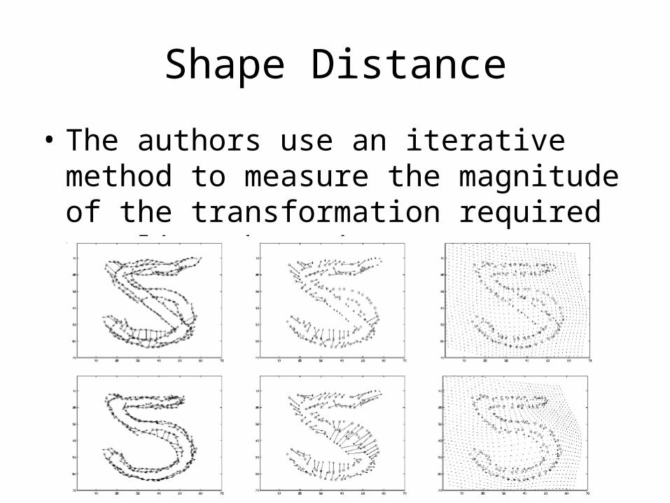
Shape Distance

• The authors use an iterative method to measure the magnitude of the transformation required to align the points

Categorization of Images

• Prototype-based approach (with k-NN)• Prototypes are chosen using k-medoids• k is initialized to the number of categories• Worst category is split until training

classification error drops below a criterion level

Application: Digit Recognition

Training set size:20,000

Test set size:10,000

Error:0.63%

Application: Breaking CAPTCHA

space

sock

92% success rate onEZ-Gimpy

Application: Breaking CAPTCHA

Must identify three words.

33% success rate on Gimpy.

Application: Trademark Retrieval

• Can be used to find different shapes with similar elements.

• Useful to determine cases of trademark infringement.

Application: 3D Object Recognition

Not the most natural application of shape contexts.

Test examples can only be matched to an image taken from a very similar angle.

Shape context conclusions

• Shape context is a local descriptor that describes a point’s location relative to its neighbors

• Good at character recognition, comparison of isolated 2D structures

• Not well suited to classification of objects with significant variance

Matching Images/Video UsingLocal Self-Similarities (2007)

• Matching Local Self-Similarities across Images and Videos– Eli Shechtman– Michal Irani

Matching Images/Video UsingLocal Self-Similarities (2007)

• All of these images contain the same object.

• The images do not share colors, textures, or edges.

Problem:

• Previous Descriptors for Image Matching:– Pixel intensity or color values of the entire image– Pixel intensity or color values of parts of the image– Texture filters– Distribution-based descriptors (e.g., SIFT)– Shape context

• All of these assume that there exists a visual property that is shared by the two images.

Solution: A “Self-Similarity” Descriptor

• The four heart images are similar only in that the local internal layouts of their self-similarities are shared.

• Video data (seen as a cube of pixels) is rife with self-similarity.

General Approach

• Our smallest unit of comparison is the “patch” rather than the pixel.

• Patches are compared to a larger, encompassing image region.

General Approach

• The comparison results in a correlation surface which determines nearby areas of the image which are similar to the current patch.

• The correlation surface is used to produce a self-similarity image descriptor for the patch.

General Approach

• For video data, the patch and region are cubes, as time is the depth dimension.

• The resulting video descriptor is cylindrical.

Descriptor Generation Process

• For every image patch q (e.g., 5x5 pixel area)– For every patch-sized area contained in the enclosing

image region (e.g., 50x50 pixel area)• Calculate SSD and determine correlation surface

• varnoise is a constant which specifies the level of acceptable photometric variation

• varauto(q) is the maximal variance of the difference of all patches near q


• Transform each correlation surface to log-polar coordinates with 80 bins (20 angles, 4 radial intervals)

• The largest value in each bin determines the entry in the descriptor.


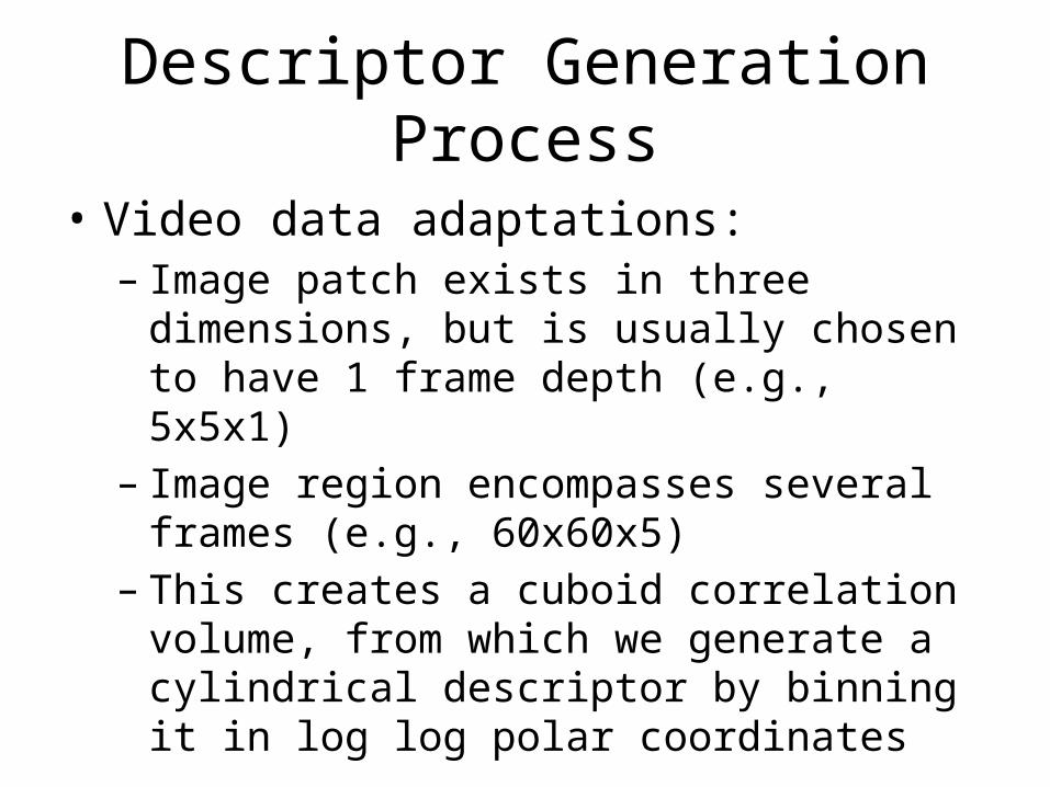
• Video data adaptations:– Image patch exists in three dimensions, but is

usually chosen to have 1 frame depth (e.g., 5x5x1)– Image region encompasses several frames (e.g.,

60x60x5)– This creates a cuboid correlation volume, from

which we generate a cylindrical descriptor by binning it in log log polar coordinates

Properties of the Self-Similarity Descriptor

• Self-similarity descriptors are local features• The log-polar representation allows for small

affine deformations (like for shape contexts)• The nature of binning allows for non-rigid

deformations• Using patches instead of pixels captures more

meaningful patterns

Performing Shape Matching

1. Calculate self-similarity descriptors for the image at a variety of scales (gives us invariance to scale)

2. Filter out the uninformative descriptors for each scale

3. Employ probabilistic star graph model to find the probability of a pattern match at each site for each scale

4. Normalize and combine the probability maps using a weighted average

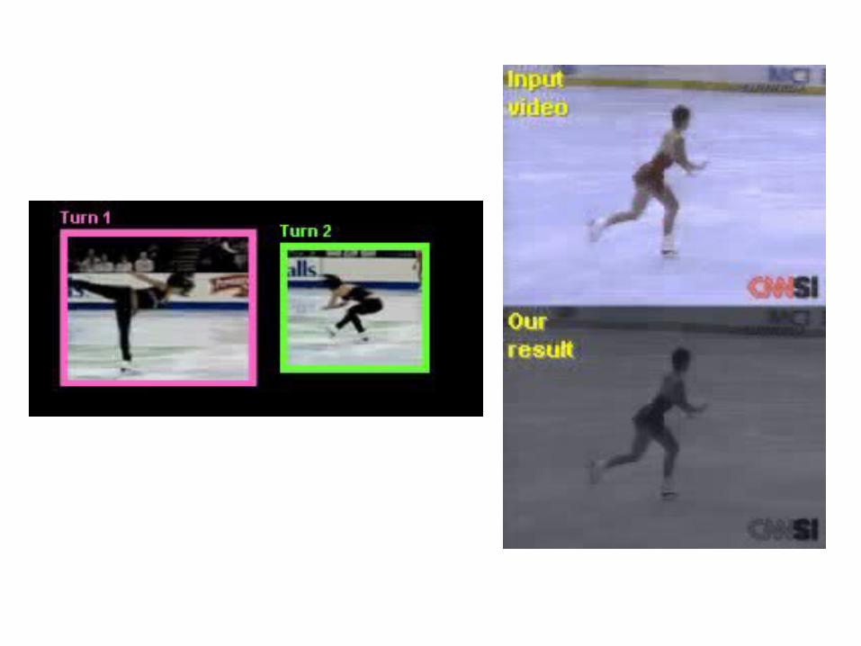
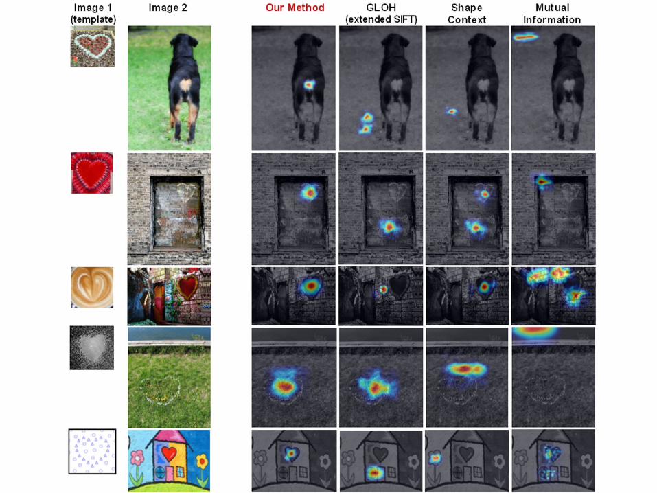
Results

• Results require only one query image which can be much smaller than the target images

• Process even works when one of the images is hand-drawn

Results

Self-Similarity Conclusions

• Can discover similar shapes in images that share no common image properties

• Requires only a single query image to perform complex shape detection

• Hand-drawn sketches are sufficient to find matches

• Video is a natural extension

The Pyramid Match Kernel (2005)

• The Pyramid Match Kernel: Discriminative Classification with Sets of Image Features– Kristen Grauman– Trevor Darrell


• Support Vector Machines– Widely used

approach to discriminative classification

– Finds the optimal separating hyperplane between two classes


• Kernels can be used to transform the feature space (e.g. XOR)

• Kernels are typically similarity measures between points in the original feature space


• Most kernels are used on fixed-length feature vectors where ordering is meaningful

• In image matching, the number of image features differ, and the ordering is arbitrary

• Furthermore, most kernels take polynomial time, which is prohibitive for image matching

Desirable characteristics in an image matching kernel

• Captures co-occurrences• Is positive-definite• Does not assume a parametric model• Can handle sets of unequal cardinality• Runs in sub-polynomial time

• No previous image matching kernels had all four of the first characteristics, and all ran in polynomial time

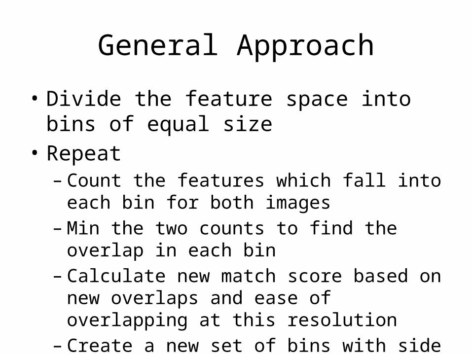
General Approach

• Divide the feature space into bins of equal size• Repeat– Count the features which fall into each bin for

both images– Min the two counts to find the overlap in each bin– Calculate new match score based on new overlaps

and ease of overlapping at this resolution– Create a new set of bins with side length double

that of the current side length

General Approach

Process

• Input space X• d-dimensional feature vectors that– are bounded by a sphere of diameter D– have a minimum inter-vector distance of

Process

• Feature Extraction Algorithm:

• H are histograms• L is the number of levels in the pyramid

Process

• Similarity between two feature sets is defined as:

• Ni is the number of new matches across all bins

• wi is the maximum distance that could exist between points that matched at this level

Process

Process

• To counteract the arbitrary nature of the bin borders, the entire process is repeated several times with the origin randomly shifted.

Partial Match Correspondences

• Unequal cardinalities are not an issue• Algorithm matches the most similar pairs first;

only the least similar features will be unmatched

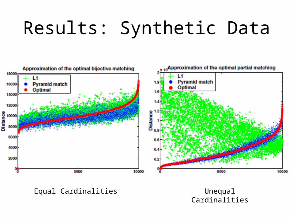
Results: Synthetic Data

Equal Cardinalities Unequal Cardinalities

Results: Object Recognition

Pyramid Kernel Conclusions

• By not searching for specific feature correspondences, the kernel can run in less than polynomial time

• Accuracy is generally higher than other kernels on both artificial and real-world data

• Can handle arbitrary-length feature sets

Spatial Pyramid Matching (2006)

• Beyond Bags of Features: Spatial Pyramid Matching for Recognizing Nature Scene Categories– Svetlana Lazebnik– Cordelia Schmid– Jean Ponce

Spatial Pyramid Matching (2006)

• Task: Whole image classification– Bag of features methods (like pyramid kernel) are

somewhat effective, but ignore feature location

• Alternate solution: Kernel-based recognition method that calculates a global rough geometric correspondence using a pyramid matching scheme

General Approach

• Similar pyramid matching scheme to previous approach, but– pyramid matching in image space– clustering in feature space

• Use training data to cluster features into M types

• Within image-space bins, count occurrences of each feature type

Process

• Algorithm parameters– M = number of feature types to learn (200)– L = levels in the pyramid (2)

• Learn M feature prototypes via k-means clustering

• Assign one of the M types to every feature value in both images

Process

• Beginning at the deepest level of the pyramid and moving to coarser levels:– Count the number of feature values of each type in each bin for each

image– Determine how many new matches there are in each bin

Results

• To classify scenes into one of N categories, we use N SVMs– Each SVM is trained to recognize a particular type

of scene– Test images are classified based on which SVM

returns the highest confidence that the test image is a member

Results

• Method performs well on similar-looking subjects, poorly on subjects with different poses/textures

Spatial Pyramid Matching Conclusions

• Makes use of positional information in addition to extracted feature values

• Has the form of an extended bag-of-features method

• Has ~80% accuracy categorizing images into 15 different classes

Images taken from• http://www.cs.sfu.ca/~mori/research/gimpy/• http://www.eecs.berkeley.edu/Research/Projects/CS/vision/shape/belongie-iccv01.ppt• http://www.wisdom.weizmann.ac.il/~vision/SelfSimilarities.html• The four papers

Shape and Matching Andrew Bender Alexander Cobian.

Documents

Transcript of Shape and Matching Andrew Bender Alexander Cobian.