Proceedings of the 2020 Conference on Empirical Methods in Natural Language Processing, pages 8485–8497,November 16–20, 2020. c©2020 Association for Computational Linguistics

8485

Sequential Modelling of the Evolution of Word Representations forSemantic Change Detection

Adam Tsakalidis1,3 Maria Liakata1,2,3

1Queen Mary University of London, London, UK2University of Warwick, Coventry, UK

3The Alan Turing Institute, London, UKatsakalidis,mliakata@turing.ac.uk

AbstractSemantic change detection concerns the taskof identifying words whose meaning haschanged over time. Current state-of-the-art ap-proaches operating on neural embeddings de-tect the level of semantic change in a wordby comparing its vector representation in twodistinct time periods, without considering itsevolution through time. In this work, we pro-pose three variants of sequential models for de-tecting semantically shifted words, effectivelyaccounting for the changes in the word repre-sentations over time. Through extensive ex-perimentation under various settings with syn-thetic and real data we showcase the impor-tance of sequential modelling of word vectorsthrough time for semantic change detection.Finally, we compare different approaches ina quantitative manner, demonstrating that tem-poral modelling of word representations yieldsa clear-cut advantage in performance.

1 Introduction

Identifying words whose lexical meaning haschanged over time is a primary area of researchat the intersection of natural language processingand historical linguistics. Through the evolution oflanguage, the task of “semantic change detection”(Tahmasebi et al., 2018; Tang, 2018; Kutuzov et al.,2018) can provide valuable insights on cultural evo-lution over time (Michel et al., 2011). Measuringlinguistic change is also relevant to understand-ing the dynamics in online communities (Danescu-Niculescu-Mizil et al., 2013) and the evolution ofindividuals (McAuley and Leskovec, 2013). Re-cent years have seen a surge in interest in this areasince researchers are now able to leverage the in-creasing availability of historical corpora in digitalform and develop models that detect the shift in aword’s meaning through time.

However, two key challenges in the field stillremain. Firstly, there is little work in existing lit-

erature on model comparison (Schlechtweg et al.,2019; Dubossarsky et al., 2019; Shoemark et al.,2019). Partially due to the lack of (longitudinal)labelled datasets, existing work assesses model per-formance mainly in a qualitative manner, withoutquantitative comparisons against prior work. There-fore, it becomes difficult to assess what constitutesan appropriate approach for semantic change de-tection. Secondly, on a methodological front, alarge body of related work detects semanticallyshifted words by pairwise comparisons of their rep-resentations in distinct time periods, ignoring thesequential modelling aspect of the task. Since se-mantic change is a time-sensitive process (Tsaka-lidis et al., 2019), considering consecutive vectorrepresentations through time – instead of two binsof word representations (Schlechtweg et al., 2018,2020) – can be crucial to improving model perfor-mance (Shoemark et al., 2019).

Here we tackle both challenges by approachingsemantic change detection as an anomaly identifica-tion task. Working on embedding representationsof words in the English language, we learn theirevolution through time via an encoder-decoder ar-chitecture. We hypothesize that once such a modelhas been successfully trained on temporally sen-sitive sequences of word representations, it willaccurately predict the evolution of the semanticrepresentation of any word through time. Wordsthat have undergone semantic change will be thosethat yield the highest errors by the prediction model.Our work makes the following contributions:

• we develop three variants of an LSTM-basedarchitecture to measure the level of semanticchange of a word by tracking its evolutionthrough time in a sequential manner: (a) aword representation autoencoder, (b) a futureword representation decoder and (c) a hybridapproach combining (a) and (b);

8486

• we show the effectiveness of our models underthorough experimentation with synthetic data;

• we compare our models against current prac-tices and competitive baselines using real data,demonstrating important gains in performanceand highlighting the importance of sequentialmodelling of word vectors through time;

• we release our code, to help set up a bench-mark for model comparison within the domainin a quantitative fashion.1

2 Related Work

One can distinguish two directions within the lit-erature on semantic change detection: (a) learn-ing word representations over discrete time inter-vals (bins) and comparing the resulting vectors and(b) jointly learning word representations acrosstime (Bamler and Mandt, 2017; Rosenfeld and Erk,2018; Yao et al., 2018; Rudolph and Blei, 2018).Such representations can be generated via differentapproaches, such as topic- (Frermann and Lapata,2016; Perrone et al., 2019), graph- (Mitra et al.,2014) and neural-based models (e.g., word2vec)– work by Tahmasebi et al. (2018) provides anoverview of such approaches. In this work wefocus on (a) due to scalability issues in learningdiachronic representations from very large corpora,as in our case, and – without loss of generality – weutilise pre-trained, neural-based representations.

Related work in (a) derives word representationsWi (i ∈ [0,..,|T − 1|]) across |T | time intervals andperforms pairwise comparisons for different valuesof i. Early work used frequency- or co-occurrence-based representations (Sagi et al., 2009; Cook andStevenson, 2010; Gulordava and Baroni, 2011; Mi-halcea and Nastase, 2012). However, leveragingword2vec-based representations (Mikolov et al.,2013) has become the common practice in recentyears. Due to the stochastic nature of word2vec,Orthogonal Procrustes (OP) (Schonemann, 1966)is often applied to the resulting vectors, aimingat aligning the pairwise representations (Kulkarniet al., 2015; Hamilton et al., 2016; Del Trediciet al., 2019; Shoemark et al., 2019; Tsakalidiset al., 2019; Schlechtweg et al., 2019). Given twoword matrices Wk, Wj at times k and j respec-tively, OP finds the optimal transformation matrixR = argmin

Ω;ΩT Ω=I

‖ΩWk −Wj‖F and the semantic

1Code is available at: https://github.com/adtsakal/semantic_change_evolution

shift level of a word w during this time intervalis defined as the cosine distance between the twoaligned matrices (Hamilton et al., 2016). By oper-ating in a linear pairwise fashion, such approachesignore the time-sensitive and possibly non-linearnature of semantic change.

By contrast, Kim et al. (2014), Kulkarni et al.(2015), Dubossarsky et al. (2019) and Shoemarket al. (2019) derive time series of a word’s levelof semantic change to detect semantically shiftedwords. Even though these methods incorporatetemporal modelling, they either rely heavily onthe linear transformation R (Kulkarni et al., 2015;Shoemark et al., 2019) or focus primarily on thegeneration of temporally-sensitive representationsas a means towards capturing semantic change(Kim et al., 2014; Dubossarsky et al., 2019). Akey contribution of our work is that we do not baseour methods on pre-defined transformations, butinstead propose a model for learning how (any typeof) pre-trained word representations vary acrosstime, effectively exploiting the full sequence of aword’s evolution.

Finally, the comparative evaluation of seman-tic change detection models is still in its infancy.Most related work assesses model performancebased on artificial tasks (Cook and Stevenson,2010; Kulkarni et al., 2015; Rosenfeld and Erk,2018; Dubossarsky et al., 2019; Shoemark et al.,2019) or on a few hand-picked examples (Sagiet al., 2009), without cross-model comparison. Therecently introduced shared tasks SemEval Task 1(Schlechtweg et al., 2020) and DIACR-Ita (Basileet al., 2020) aim at bridging this gap; however, therespective datasets consist of documents split intwo distinct time periods, thus not facilitating thestudy of the sequential nature of semantic change.Setting a benchmark for model comparison withreal-world and sequential word representations iscrucial in this field.

3 Methods

We formulate semantic change detection as ananomaly detection task in the evolution of pre-trained word embeddings. We assume that pre-trained word vectorsWt ∈ [W0, ...,W|T−1|], whereWt ∈ R|V |×d (|V |: vocabulary size; d: word repre-sentation size) in a historical corpus over |T | timeperiods, evolve according to a non-linear function

8487

f(Wt).2 By approximating f , we obtain the levelof semantic shift of a word w at time t by measur-ing the similarity between its word representationwt against f(wt). A low similarity score for agiven word implies an inaccurate model prediction(anomaly) and thus a high level of semantic changefor the given word. Therefore, we can obtain aranking of the words based on their semantic shiftlevel by ordering them in ascending order of theirsimilarity scores between wt and f(wt). We ap-proximate f via temporally sensitive deep neuralmodels: (a) an autoencoder, which aims to recon-struct a word’s trajectory up to a given point in timei [w0, ..., w|i|] (section 3.1); and (b) a future pre-dictor, which aims to predict future representationsof the word [w|i+1|, ..., w|T−1|] (section 3.2). Thetwo models can be trained individually or (c) in ajoint multi-task setting (section 3.3). These modelsbenefit from accounting for sequential word rep-resentations across time [W0, ...,W|T−1|], whichis better suited for detecting semantically shiftedwords compared to the common practice of com-paring only the first and last word representations[W0, W|T−1|] (Shoemark et al., 2019).

EncodedSequence

§3.1: Reconstructing Word Representations

§3.2: Predicting Future Word Representations

W0 W1 Wi−2 Wi−1

Wr0 Wri−1 Wf

i WfT−1

LSTM

s LSTMs

LSTM

s

Dense Dense

Figure 1: Overview of our proposed model: the se-quence of the representation of a set of word vectors(vocabulary) over different time steps W0:i−1 is en-coded through two LSTM layers and then passed overto a reconstruction (3.1) decoder and a future predictiondecoder (3.2). The model is trained by utilising eitherdecoder in isolation, or both of them in parallel (3.3).

3.1 Reconstructing Word RepresentationsGiven an input sequence of vectors representingthe words in a vocabulary across i points in time

2Note: t in Wt indicates the time period from when theassociated pre-trained word vectors are taken (e.g., year 2000).

W0:i−1 = [W0,W1, ...,Wi−1], the goal of theautoencoder is to reconstruct the input sequenceW0:i−1. Since the task of semantic change includesa natural temporal dimension, we model our au-toencoder via RNNs (see Figure 1). The encoderis composed of two LSTM layers (Hochreiter andSchmidhuber, 1997) with Dropout layers operatingon their outputs, for regularisation (Srivastava et al.,2014). The first layer encodes the input sequenceof W0:i−1 and returns the hidden states as input tothe second layer. The output of the second layeris the final encoded state, which is then copied |i|times and fed as input to the decoder. The decoderhas the same architecture as the encoder, albeit withadditional dense layers on top of the second LSTMlayer to make the final reconstruction W r

0:i−1 onthe |i| time steps. The model is trained by minimis-ing the mean squared error (MSE) loss function:

Lr =1

i

i−1∑j=0

MSE(Wj ,Wrj ). (1)

After training, the words that yield the highest errorrates in a given test set of word representationsthrough time are considered to be the ones whosesemantics have changed the most during the giventime period. This is compatible with prior workbased on word alignment (Hamilton et al., 2016;Tsakalidis et al., 2019), where the alignment errorof a word indicates its level of semantic change.

3.2 Predicting Future Word Representations

Reconstructing the word vectors can reveal whichwords have changed their semantics in the past(i.e., up to time i− 1, see 3.1). If we are interestedin predicting changes in the semantics of futureword representations (i.e., after time i − 1), wecan consider a future word representation predic-tion task: given the sequence of past word repre-sentations W0:i−1 = [W0,W1, ...,Wi−1] over thefirst i time points, we predict the future represen-tations of the words in the vocabulary Wi:T−1 =[Wi,Wi+1, ...,WT−1], for a sequence of overalllength |T | (see Figure 1). We follow the samemodel architecture as in section 3.1, with the onlydifference being the number of time steps (T − i)used in the decoder to make |T − i| predictions.The model is trained using the loss function Lf :

Lf =1

T − i

T−1∑j=i

MSE(Wj ,Wfj ). (2)

8488

3.3 Joint Model

The two models can be combined into a joint one,where, given an input sequence of representationsof the vocabulary W0:i−1 over i points in time, thegoal is both to (a) reconstruct the input sequenceand (b) predict the future word |T − i| representa-tions Wi:T−1. The complete model architecture isprovided in Figure 1: the encoder is identical to theone used in 3.1 and 3.2. However, the bottleneck isnow copied |T | times and passed to the decoders ofthe reconstruction (|i| times) and future prediction(|T − i| times). The loss function Lrf here is thesummation of the individual losses in Eq. 1 and 2:

(3)

Lrf =1

i

i−1∑j=0

MSE(Wj ,Wrj )

+1

T − i

T−1∑j=i

MSE(Wj ,Wfj ).

There are two main reasons for modelling semanticchange in this multi-task setting. Firstly, we benefitfrom the finer granularity of the two decoders dueto their handling of only part of the sequence in amore fine-grained manner, compared to the indi-vidual task models. Secondly, the joint model isinsensitive to the value of i in Eq. 3 compared toEq. 1 and 2, as discussed next.

3.4 Model Equivalence

The three models perform different operations;however, setting the operational time periods appro-priately in Eq. 1-3 can result in model equivalence(i.e., performing the same task). Specifically, todetect the words whose semantics have changedduring [0, T − 1], the autoencoder (Eq. 1) needsto be fed and reconstruct the full sequence across[0, T − 1] (i.e., i=T -1). Reducing this interval (re-ducing i) would limit its operational time period.On the contrary, an increase in the value of i inEq. 2 of the future prediction model shortens thetime period during which it can detect the wordswhose semantics have changed the most – to detectthe words whose semantics have changed withinthe full sequence [1, T − 1], it requires only theword representations W0 in the first time interval.Therefore, setting the parameter i can be crucial forthe performance of the individual models. By con-trast, the joint model in section 3.3 is able to detectthe words that have undergone semantic change, re-gardless of the value of i (see Eq. 3), since it is still

able to operate on the full sequence – we showcasethese effects in section 5.2.

4 Experiments with Synthetic Data

Tasks run on artificial data have been used forevaluation purposes in related work (Gale et al.,1992; Schutze, 1998; Cook and Stevenson, 2010;Kulkarni et al., 2015; Rosenfeld and Erk, 2018; Du-bossarsky et al., 2019; Shoemark et al., 2019). Inthis section, we work with artificial data as a proof-of-concept of our proposed models – we compareagainst state-of-the-art and other baseline methodswith real data in the next section. Here we employa longitudinal dataset of word representations (4.1)and artificially alter the representations of a smallset of words across time (4.2). We then train (4.3)our models and evaluate them on the basis of theirability to identify those words that have undergone(artificial) semantic change (4.4).

4.1 Dataset

We employ the UK Web Archive dataset (Tsaka-lidis et al., 2019), which contains 100-dimensionalrepresentations of 47.8K words for each year inthe period 2000-2013. These were obtained by em-ploying word2vec (i.e., skip-gram with negativesampling (Mikolov et al., 2013)) on the documentspublished in each year independently. Note that ourmodels can be applied to any type of pre-trainedembeddings. Each year corresponds to a time stepin our modelling. The dataset contains 65 wordswhose meaning has changed within 2001-13, asindicated by the Oxford English Dictionary. Theseare removed for the purposes of this section, toavoid interference with the artificial data modeling.We use one subset (80%) of the remaining longitu-dinal word representations for training our modelsand the rest (20%) for evaluation purposes.

4.2 Artificial Examples of Semantic Change

We generate artificial examples of words withchanging semantics, by following a paradigm in-spired by Rosenfeld and Erk (2018). We uniformlyat random select 5% of the words in the test set toalter their semantics. For every selected “source”word α, we select a “target” word β (details aboutthe selection process of β are provided in the nextparagraph). We then alter the representation w(α)

t

of the source word α at each point in time t sothat it shifts towards the representation w(β)

t of thetarget word at this point in time as:

8489

w∗(α)t = λtw

(α)t + (1− λt)w(β)

t . (4)

Following Rosenfeld and Erk (2018), we model λtvia a sigmoid function. λt receives values within[0, 1] and acts as a decay function that controls thespeed of change in the source word’s semantics to-wards the target. Thus, the semantic representationof α is not altered during the first time points andthen it gradually shifts towards the representationof β (for middle values of t), where it stabilizes to-wards the last time points. Since the duration of thesemantic shift of a word may vary, we experimentunder different scenarios (see “Conditioning on Du-ration of Change” below). Alternative modellingapproaches of artificial semantic change have beenpresented in Shoemark et al. (2019) – e.g., forcinga word to acquire a new sense while also retainingits original meaning. We opted for the “stronger”case of semantic shift (Eq. 4) as a proof-of-conceptfor our models. In section 5 we experiment withreal-world data, without any assumptions about theform of the function underlying semantic change.

Conditioning on Target Words The selectionof the target words should be such that they allowthe representation of the source word to changethrough time (Dubossarsky et al., 2019). This willnot be the case if we select a pair of α, β source,target words whose representations are very simi-lar (e.g., synonyms). Thus, for each source wordα we select uniformly at random a target word βs.t. the cosine similarity of their representations atthe initial time point (i.e., in the year 2000) fallswithin a certain range (c − 0.1, c]. Higher val-ues of c enforce a lower semantic change levelfor α through time, since its representation will beshifted towards a similar word β, and vice versa. Toassess model performance across different levelsof semantic change, we experiment with varyingc = 0.0, 0.1, ..., 0.5.

Conditioning on Duration of Change The du-ration of semantic change affects the value of λt inEq. 4. We conventionally set λ07 = 0.5, s.t. the ar-tificial word representation w∗(α)

07 of a source wordα in 2007 (i.e., the midpoint between 2001-2013)to be equal to 0.5(w

(α)07 + w

(β)07 ). We then experi-

ment with four different duration [start, end] rangesfor the semantic change: (a) “Full” [2001-13], (b)“Half” [2005-10], (c) “OT” (One-Third) [2006-09]and (d) “Quarter” [2007-08]. A longer lasting se-mantic change duration implies a smoother transi-tion of word α towards the meaning of word β, and

vice versa (see Figure 2). By generating syntheticexamples of varying semantic change duration weare able to measure model performance under dif-ferent conditions.

Figure 2: The different functions used to model λt inEq. 4, indicating the speed and duration of semanticchange of our synthetic examples (see section 4.2).

4.3 Artificial Data ExperimentOur task is to rank the words in the test set bymeans of their level of semantic change. We firsttrain our three models on the training set and thenwe apply them on the test set. Finally, we measurethe level of semantic change of a word by means ofthe average cosine similarity between the predictedand actual word representations at each time stepof the decoder. Model performance is assessed viarank-based metrics (Basile and McGillivray, 2018;Tsakalidis et al., 2019; Shoemark et al., 2019).

Model Training We define and train our modelsas follows:

• seq2seqr: the autoencoder (section 3.1) re-ceives and reconstructs the full sequence ofthe word representations in the training set:[W00, ...,W13]→ [W r

00, ...,Wr13].

• seq2seqf : the future prediction model (sec-tion 3.2) receives the representation of thewords in the training set in the year 2000and learns to predict the rest of the sequence:[W00]→ [W f

01, ...,Wf13].

• seq2seqrf : the multi-task model (sec-tion 3.3) is fed with the first half of the se-quence of the word representations in the train-ing set and jointly learns to (a) reconstruct theinput sequence and (b) predict the word rep-resentations in the future: [W00, ...,W06] →[W r

00, ...,Wr06], [W f

07, ...,Wf13].

8490

We have a different number of timesteps forseq2seqr and seq2seqf in their input, so thatthe decoder in each model operates on the maxi-mum possible output sequence, thus exploiting thesemantic change of the words over the whole timeperiod (see section 3.4). seq2seqrf is expectedto be insensitive to the number of input time steps,therefore we conventionally set it to half of theoverall sequence. We keep 25% of our training setfor validation purposes and train our models usingthe Adam optimiser (Kingma and Ba, 2015). Weselect the best parameters after 25 trials using theTree of Parzen Estimators algorithm of the hyper-opt module (Bergstra et al., 2013), by means ofthe maximum average (i.e., per time step) cosinesimilarity in the validation set.3

Testing and Evaluation After training, eachmodel is applied to the test set, yielding its pre-dictions for every word through time.4 The levelof semantic change of a word is then calculatedvia the average cosine similarity between the ac-tual and the predicted word representations throughtime, with higher values indicating a better modelprediction (thus, a lower level of semantic change).The words are ranked on ascending order of theiraverage cosine similarity, with the first ranks indi-cating words whose representations have changedthe most (low cosine similarity). For evaluation,similarly to Tsakalidis et al. (2019), we employ theaverage rank across all of the semantically changedwords (in %, denoted here as µr), with lower scoresindicating a better model. We prefer µr to the meanreciprocal rank, because the latter emphasises thefirst rankings. Since semantic change detection isan under-explored task in quantitative terms, weaim at getting better insights on model performanceby working with an averaging metric. For the samereason we avoid using classification-based metricsthat are based on a cut-off point (e.g., recall at k(Basile and McGillivray, 2018)). We do make useof such metrics in the cross-model comparison withreal data (section 5.2).

4.4 Results

Model Comparison Figure 3 presents the resultsof the three models on our synthetic data acrossall (c, λ) combinations. seq2seqrf performs

3For the complete list of parameters that were tested in allmodels/baselines in our work, refer to Appendix A.

4Note that the future prediction model does not make aprediction for the first time step (year 2000).

consistently better than the individual (seq2seqr,seq2seqf ) models in µr, showing that combiningthe two models under a multi-task setting benefitsfrom the joint and finer-grained parameter tuning ofthe two components. seq2seqr performs slightlybetter than seq2seqf , probably due to the autoen-coder having to output a longer sequence (i.e., duetoW r

00), which helps explore the temporal variationof the words more effectively.

Figure 4 shows the cosine similarity betweenthe predicted and actual representation of eachsynthetic word per time step for the “Full” casewhen c=0.0 (highest level of change, see sec-tion 4.2). seq2seqr reconstructs the input se-quence of synthetic examples more accurately thanthe future prediction component (average cosinesimilarity per year (avg cos): .65 vs .50). Itparticularly manages to reconstruct the syntheticword representations during the years 2006-2008(avg cos06:08=.75), which are the points whenλt varies more rapidly (see Figure 2); however,it fails to reconstruct equally well their repre-sentations before (avg cos00:05= .65) and after(avg cos09:13= .59) this sharp change. On the con-trary, seq2seqf predicts more accurately the syn-thetic word representations during the first years(avg cos01:05 = .74), when the change in their se-mantics is minor, but (correctly) fails after thesemantic change is almost complete (i.e., whenλt ≤ .25, avg cos09:13= .24). seq2seqrf bene-fits from the individual components’ advantage: itappropriately reconstructs the artificial examplesin the first years (avg cos00:05 = .85) so that theirsemantic shift is highlighted more clearly during(avg cos06:08= .62) and after the process is almostcomplete (avg cos09:13= .26). Finally, avg cos inseq2seqrf highly correlates with λt (ρ=.987),potentially providing insights on how to measurethe speed of semantic change of a word.

Effect of Conditioning Parameters Regardlessof the duration of the semantic change process, anincrease in the value of c results in model perfor-mance degradation. This is expected, since the in-crease of c implies that the level of semantic changeof the source words is lower, as discussed in 4.2,thus making the task of detecting them more diffi-cult. Nevertheless, our worst performing model inthe most challenging setting (c=0.5, Full, seq2seqf )achieves µr=28.17, which is clearly better than theµr expected by a random baseline (µr=50.00).

The decrease of the duration of semantic change

8491

(a) Full (b) Half (c) OT (d) Quarter

Figure 3: µr of our models on the synthetic dataset for different values of the threshold c (x-axis) and the differentperiods of duration of semantic change (one per chart, see 4.2). Lower µr values indicate a better performance.

(a) seq2seqr (b) seq2seqf (c) seq2seqrf

Figure 4: Cosine similarity between the actual andthe predicted vectors of the synthetic words that haveundergone artificial semantic change (rows), per year(columns). Light colours indicate inaccurate model pre-dictions of the word vectors – i.e., indicating that theassociated words have undergone semantic change.

has a positive effect on our models (see Figure 3).This is more evident in the cases of high value of c,where seq2seqr (µr: 26.09-18.21 in the Full-to-Quarter cases), seq2seqf (µr: 28.17-22.48) andseq2seqrf (µr:20.38-13.09) show clear gains inperformance. This indicates that our models cancapture the semantic change in small subsequencesof the time-series. Studying this effect in datasetsof longer duration is an important future direction.

5 Model Comparison with Real Data

5.1 Experimental SettingWe approach the task in a rank-based manner, asin section 4. However, here we are interested indetecting real-world examples of semantic changein words and comparing our models against strongbaselines and current practices.

Data and Task We employ the UK Web Archivedataset (see section 4.1). We keep the same 80/20train/test split as in section 4 and incorporate inthe test set the 65 words with known changes inmeaning according to the Oxford English Dictio-nary. We train our models as in section 4.3, aimingat detecting the 65 words in the test set. We useµr (as in section 4) and recall at k (Rec@k, k=5%,10%, 50%) as our evaluation metrics. We refrain

from using precision at k, since Oxford EnglishDictionary is not expected to have a full coverageof the semantically shifted words. Lower µr andhigher Rec@k scores indicate better models.

Models We compare the three variants from sec-tion 3 against four types of baselines:– A random word rank generator (RAND). We reportaverage metrics after 1K runs on the test set.

– Variants of Procrustes Alignment, as a commonpractice in past work: Given word representationsin two different years [W0, Wi] centered aroundthe origin and s.t. tr(WkW

Tk ) = 1, PROCR trans-

forms Wi into W ∗i s.t. the squared differencesbetween W0 and W ∗i are minimised. We alsouse the PROCRk and PROCRkt variants (Tsakalidiset al., 2019), which first detect the k most stablewords across either [W0, Wi] (PROCRk) or [W0, ...,WT−1] (PROCRkt) to learn the alignment and thentransform Wi into W ∗i . Words are ranked based onthe cosine distance between [W0, W ∗i ].

– Models leveraging the first and last word represen-tations only. We use a Random Forest (Breiman,2001) regression model (RF) that predicts Wi,given W0. We also use the same architectures pre-sented in sections 3.1-3.2, trained on [W0, Wi] (ig-noring the full sequence): LSTMr reconstructs thesequence [W0, Wi]; LSTMf predictsWi, givenW0,similarly to RF. Words are ranked in ascending or-der of the (average, for LSTMr) cosine similaritybetween their predicted and actual representations.– Models operating on the time series of distances.Given a sequence of vectors [W0, ..., Wi], we con-struct the time series of cosine distances that resultby PROCR. Then, we use two global trend models(Shoemark et al., 2019): GTc ranks the words bymeans of the absolute value of the Pearson corre-lation of their time series; GTβ fits a linear regres-sion model for every word and ranks the wordsby the absolute value of the slope. Finally, we

8492

µr Rec@5 Rec@10 Rec@50’00-’13 avg±std ’00-’13 avg±std ’00-’13 avg±std ’00-’13 avg±std

[=[Pa

stW

ork/

Bas

elin

es! RAND 49.97 50.01±0.04 5.00 4.99±0.03 10.01 9.98±0.04 50.02 49.97±0.08

PROCR 30.63 28.51±2.68 18.46 14.32±5.00 27.69 29.94±4.64 78.46 80.47±3.79PROCRk 31.01 28.67±2.73 21.54 14.91±4.75 27.69 30.18±4.42 75.38 79.53±4.50PROCRkt 31.91 28.47±2.85 20.00 14.32±4.23 27.69 28.88±4.45 70.77 80.00±4.53RF 30.01 30.45±4.15 10.77 15.62±4.30 21.54 27.46±7.16 78.46 77.63±6.42LSTMr 27.87 27.83±2.65 12.31 15.98±5.94 29.23 30.30±6.39 80.00 80.12±4.72LSTMf 28.62 28.61±3.47 16.92 17.40±5.60 32.31 31.83±6.07 76.92 78.82±4.83GTc 47.87 44.04±1.54 7.69 7.41±2.26 16.92 14.13±3.76 52.31 57.90±2.94GTβ 38.09 36.16±1.74 13.85 14.83±4.14 24.62 23.36±3.94 66.15 69.37±3.26PROCR˙∗ 25.01 27.99±3.03 21.54 15.15 ±4.52 32.31 28.40±3.75 81.54 80.24±3.49

[=[

Our

s! seq2seqr 24.75 28.36±3.38 21.54 19.05±4.47 38.46 29.94±6.64 84.62 81.42±4.64seq2seqf 23.86 27.17±4.16 26.15 22.01±6.72 46.15 34.32±10.13 84.62 81.18±5.07seq2seqrf 24.28 24.29±0.67 29.23 25.77±2.28 36.92 39.49±2.11 84.62 85.00±1.16

Table 1: Model comparison when operating on the entire time sequence(2000-13) and averaged across time (2000-01, ..., 2000-13). Past work andbaseline models shown in the table are defined in section 5.1 (“Models”).

Figure 5: µr of our models forvarying value of i (Eq. 1–3).5Forthe complete results, refer to Ap-pendix B.

employ PROCR∗, ranking words based on the aver-age cosine distance within [0, i]; this is similar tothe “Mean Distances” model used in Rodina et al.(2019), with the difference that the distances attime point i are calculated by measuring the cosinedistance resulting from the alignment against theinitial time point 0 and not against i− 1.6

We report the performance of the models (a)when they operate on the full interval [2000-13]and (b) averaged across all intervals [2000-01, ...,2000-13]. In (b), our models use additional (fu-ture) information compared to our baselines; whenseq2seqf is fed with the word sequences of[2000, 2001], it makes a prediction for the years[2002, ..., 2013] – such information cannot be lever-aged by the baselines. Thus, for (b), we only per-form intra-model (and intra-baseline) comparisons.

5.2 Results

Our models vs baselines Results are shown inTable 1. The three proposed models consistentlyachieve the lowest µr and highest Rec@k whenworking on the whole time sequence (’00-’13columns). The comparison between seq2seqr,LSTMr and seq2seqf , LSTMf in the years2000-13 showcases the benefit of modelling thefull sequence of the word representations acrosstime, compared to using the first and last represen-tations only. Our models provide a relative boost of4.6% in µr and [35.7%, 42.8%, 5.8%] in Rec@k(for k=[5, 10, 50]) compared to the best perform-

5Example (2005 in x-axis): The sequence of the wordrepresentations until 2005 is the input to all of our models.Then, seq2seqr reconstructs the word representations up to2005, seq2seqf predicts the future representations (2006,..., 2013) and seq2seqrf performs both tasks jointly.

6We refrain from evaluating the GT models when i ≤2,due to the very short time interval that does not allow for corre-lations to appear in the data, leading to very poor performance.

ing baseline. seq2seqf and seq2seqrf modelsoutperform the autoencoder (seq2seqr) in mostmetrics, while seq2seqrf yields the most stableresults across all runs. We explore these differencesin detail in the last paragraph of this section.

Intra-baseline comparison Models operatingonly on the first and last word representations fail toconfidently outperform the Procrustes-based base-lines, demonstrating again the weakness of operat-ing in a non-sequential manner. The LSTM mod-els achieve low µr on the 2000-13 experiments;however, the difference with the rest of the base-lines in µr across all years is negligible. The intra-Procrustes model comparison shows that the benefitof selecting a few anchor words to learn a betteralignment (PROCRk, PROCRkt) shown in Tsaka-lidis et al. (2019) in examining semantic changeover two consecutive years might not apply whenexamining a longer time period. Finally, contrary toShoemark et al. (2019), we find that time sensitivemodels operating on the word distances across time(GTc, GTβ) perform worse than the baselines thatleverage only the first and last word representations.This difference is attributed to the low number oftime steps in our dataset that does not allow the GTmodels to exploit long-term correlations (i.e., con-sidering the average distance across time (PROCR∗)performs better), but also highlights the importanceof leveraging the full word sequence across time.

Effect of input/output lengths Figure 5 showsthe µr of our three variants when we alter the lengthof the input and output (see section 3.4). The per-formance of seq2seqr increases with the inputsize since by definition the decoder is able to de-tect words whose semantics have changed over alonger period of time (i.e., within [2000, i], withi increasing), while also modelling a longer se-

8493

Figure 6: Cosine distances (actual vs predicted vectors)of each semantically shifted word (as indicated by theOxford English Dictionary), per year. Lighter coloursindicate better model performance – thus, lower levelof semantic change predicted by our joint model.

quence of a word’s representation through time.On the contrary, the performance of seq2seqfincreases alongside the decrease of the numberof input time steps. This is expected since, as idecreases, seq2seqf encodes a shorter input se-quence and the decoding (and hence the semanticchange detection) is applied on the remaining (andincreased number of) time steps within [i+1, 2013].These findings provide empirical evidence that bothmodels can achieve better performance if trainedover longer sequences of time steps. Finally, thestability of seq2seqrf showcases its input length-invariant nature, which is also clearly evident inall of the averaged results (standard deviation inavg±std columns) in Table 1: in its worst perform-ing setting, seq2seqrf still manages to achieve

results that are close to the best performing model(µr=25.17, Rec@k=[21.54, 36.92, 83.08] for thethree thresholds) and always better (or equal to)the best performing baseline shown in Table 1 inRec@k. This is a very attractive aspect of themodel as it removes the need to manually definethe number of time steps to be fed to the encoder.

Words with shifted meaning Figure 6 showsthe cosine distances between the actual and pre-dicted vectors of the 65 words that acquired anew meaning between 2001-2013. The distancesare calculated by applying the seq2seqrf model(trained as in section 4.3) on the test set. The wordsare ranked based on their average cosine distancethroughout the years such that the words in the firstrows form more challenging examples for detect-ing their semantic shift. Despite that some of thesewords have acquired an additional meaning in thecontext of social networks (e.g., “like”, “unlike”),this is not effectively captured by their vectors. Util-ising contextual representations (Giulianelli et al.,2020) in our models can be more effective for cap-turing such cases in future work.

6 Conclusion and Future Work

We introduce three sequential models for semanticchange detection that effectively exploit the fullsequence of a word’s representations through timeto determine its level of semantic change. Throughextensive experiments on synthetic and real data weshowcase the effectiveness of the proposed mod-els under various settings and in comparison tostate-of-the-art on the UK Web Archive dataset.Importantly, we show that their performance in-creases alongside the duration of the time periodunder study, confidently outperforming competitivemodels and common practices on semantic change.

Future work can use anomaly detection ap-proaches operating on our model’s predicted wordvectors to detect anomalies in a word’s represen-tation across time. We also plan to investigate dif-ferent architectures, such as Variational Autoen-coders (Kingma and Welling, 2014), and incorpo-rate contextual representations (Devlin et al., 2019;Hu et al., 2019) to detect new senses of words. Alimitation of our work is that it has been tested ona single dataset, where 65 words have undergonesemantic change; testing our models in datasets ofdifferent duration and in different languages willprovide clearer evidence of their effectiveness.

8494

Acknowledgements

This work was supported by The Alan Turing In-stitute (grant EP/N510129/1) and by a Turing AIFellowship to Maria Liakata, funded by the De-partment of Business, Energy & Industrial Strat-egy. The authors would like to thank StephenClark, Mihai Cucuringu, Elena Kochkina, BarbaraMcGillivray, Federico Nanni, Nicole Peinelt andthe anonymous reviewers for their valuable feed-back.

ReferencesRobert Bamler and Stephan Mandt. 2017. Dynamic

Word Embeddings. In Proceedings of the 34th Inter-national Conference on Machine Learning-Volume70, pages 380–389. JMLR. org.

Pierpaolo Basile, Annalina Caputo, Tommaso Caselli,Pierluigi Cassotti, and Rossella Varvara. 2020.Overview of the EVALITA 2020 Diachronic Lexi-cal Semantics (DIACR-Ita) Task. In Proceedings ofthe 7th evaluation campaign of Natural LanguageProcessing and Speech tools for Italian (EVALITA2020), Online. CEUR.org.

Pierpaolo Basile and Barbara McGillivray. 2018. Ex-ploiting the Web for Semantic Change Detection.In International Conference on Discovery Science,pages 194–208. Springer.

James Bergstra, Daniel Yamins, and David Daniel Cox.2013. Making a Science of Model Search: Hyper-parameter Optimization in Hundreds of Dimensionsfor Vision Architectures. pages 115–123.

Leo Breiman. 2001. Random Forests. Machine Learn-ing, 45(1):5–32.

Paul Cook and Suzanne Stevenson. 2010. Automati-cally Identifying Changes in the Semantic Orienta-tion of Words. In Proceedings of the Seventh confer-ence on International Language Resources and Eval-uation.

Cristian Danescu-Niculescu-Mizil, Robert West, DanJurafsky, Jure Leskovec, and Christopher Potts.2013. No Country for Old Members: User Lifecy-cle and Linguistic Change in Online Communities.In Proceedings of the 22nd International Conferenceon World Wide Web, pages 307–318. Association forComputing Machinery.

Marco Del Tredici, Raquel Fernandez, and GemmaBoleda. 2019. Short-Term Meaning Shift: A Dis-tributional Exploration. In Proceedings of the 2019Conference of the North American Chapter of theAssociation for Computational Linguistics: HumanLanguage Technologies, Volume 1 (Long and ShortPapers), pages 2069–2075.

Jacob Devlin, Ming-Wei Chang, Kenton Lee, andKristina Toutanova. 2019. BERT: Pre-training ofDeep Bidirectional Transformers for Language Un-derstanding. In Proceedings of the 2019 Conferenceof the North American Chapter of the Associationfor Computational Linguistics: Human LanguageTechnologies, Volume 1 (Long and Short Papers),pages 4171–4186.

Haim Dubossarsky, Simon Hengchen, Nina Tahmasebi,and Dominik Schlechtweg. 2019. Time-Out: Tem-poral Referencing for Robust Modeling of LexicalSemantic Change. In Proceedings of the 57th An-nual Meeting of the Association for ComputationalLinguistics, pages 457–470.

Lea Frermann and Mirella Lapata. 2016. A BayesianModel of Diachronic Meaning Change. Transac-tions of the Association for Computational Linguis-tics, 4:31–45.

William A Gale, Kenneth W Church, and DavidYarowsky. 1992. Work on statistical methods forword sense disambiguation. In Working Notes of theAAAI Fall Symposium on Probabilistic Approachesto Natural Language, volume 54, page 60.

Mario Giulianelli, Marco Del Tredici, and RaquelFernandez. 2020. Analysing Lexical SemanticChange with Contextualised Word Representations.In Proceedings of the 58th Annual Meeting of theAssociation for Computational Linguistics, Online.Association for Computational Linguistics.

Kristina Gulordava and Marco Baroni. 2011. A distri-butional similarity approach to the detection of se-mantic change in the Google Books Ngram corpus.In Proceedings of the GEMS 2011 Workshop on Ge-ometrical Models of Natural Language Semantics,pages 67–71.

William L Hamilton, Jure Leskovec, and Dan Jurafsky.2016. Diachronic Word Embeddings Reveal Statis-tical Laws of Semantic Change. In Proceedings ofthe 54th Annual Meeting of the Association for Com-putational Linguistics (Volume 1: Long Papers), vol-ume 1, pages 1489–1501.

Sepp Hochreiter and Jurgen Schmidhuber. 1997.Long Short-Term Memory. Neural Computation,9(8):1735–1780.

Renfen Hu, Shen Li, and Shichen Liang. 2019. Di-achronic Sense Modeling with Deep ContextualizedWord Embeddings: An Ecological View. In Pro-ceedings of the 57th Annual Meeting of the Asso-ciation for Computational Linguistics, pages 3899–3908.

Yoon Kim, Yi-I Chiu, Kentaro Hanaki, Darshan Hegde,and Slav Petrov. 2014. Temporal Analysis ofLanguage through Neural Language Models. InProceedings of the ACL 2014 Workshop on Lan-guage Technologies and Computational Social Sci-ence, pages 61–65.

8495

Diederik P. Kingma and Jimmy Ba. 2015. Adam: AMethod for Stochastic Optimization. In 3rd Inter-national Conference on Learning Representations,ICLR 2015, Conference Track Proceedings.

Diederik P. Kingma and Max Welling. 2014. Auto-Encoding Variational Bayes. In 2nd InternationalConference on Learning Representations, ICLR2014, Conference Track Proceedings.

Vivek Kulkarni, Rami Al-Rfou, Bryan Perozzi, andSteven Skiena. 2015. Statistically significant de-tection of linguistic change. In Proceedings of the24th International Conference on World Wide Web,pages 625–635. International World Wide Web Con-ferences Steering Committee.

Andrey Kutuzov, Lilja Øvrelid, Terrence Szymanski,and Erik Velldal. 2018. Diachronic Word Embed-dings and Semantic Shifts: A Survey. In Proceed-ings of the 27th International Conference on Com-putational Linguistics, pages 1384–1397.

Julian John McAuley and Jure Leskovec. 2013. FromAmateurs to Connoisseurs: Modeling the Evolutionof User Expertise through Online Reviews. In Pro-ceedings of the 22nd International Conference onWorld Wide Web, pages 897–908. Association forComputing Machinery.

Jean-Baptiste Michel, Yuan Kui Shen, Aviva PresserAiden, Adrian Veres, Matthew K Gray, Joseph PPickett, Dale Hoiberg, Dan Clancy, Peter Norvig,Jon Orwant, et al. 2011. Quantitative Analysis ofCulture Using Millions of Digitized Books. Science,331(6014):176–182.

Rada Mihalcea and Vivi Nastase. 2012. Word EpochDisambiguation: Finding how Words Change overTime. In Proceedings of the 50th Annual Meeting ofthe Association for Computational Linguistics (Vol-ume 2: Short Papers), pages 259–263.

Tomas Mikolov, Ilya Sutskever, Kai Chen, Greg S Cor-rado, and Jeff Dean. 2013. Distributed Representa-tions of Words and Phrases and their Composition-ality. In Advances in Neural Information ProcessingSystems, pages 3111–3119.

Sunny Mitra, Ritwik Mitra, Martin Riedl, Chris Bie-mann, Animesh Mukherjee, and Pawan Goyal. 2014.That’s sick dude!: Automatic identification of wordsense change across different timescales. In Pro-ceedings of the 52nd Annual Meeting of the Associa-tion for Computational Linguistics (Volume 1: LongPapers), pages 1020–1029.

Valerio Perrone, Marco Palma, Simon Hengchen,Alessandro Vatri, Jim Q Smith, and BarbaraMcGillivray. 2019. GASC: Genre-Aware SemanticChange for Ancient Greek. In Proceedings of the1st International Workshop on Computational Ap-proaches to Historical Language Change, pages 56–66.

Julia Rodina, Daria Bakshandaeva, Vadim Fomin, An-drey Kutuzov, Samia Touileb, and Erik Velldal.2019. Measuring Diachronic Evolution of Evalua-tive Adjectives with Word Embeddings: the Case forEnglish, Norwegian, and Russian. In Proceedingsof the 1st International Workshop on ComputationalApproaches to Historical Language Change, pages202–209.

Alex Rosenfeld and Katrin Erk. 2018. Deep NeuralModels of Semantic Shift. In Proceedings of the2018 Conference of the North American Chapter ofthe Association for Computational Linguistics: Hu-man Language Technologies, Volume 1 (Long Pa-pers), pages 474–484.

Maja Rudolph and David Blei. 2018. Dynamic Embed-dings for Language Evolution. In Proceedings of the2018 World Wide Web Conference on World WideWeb, pages 1003–1011. International World WideWeb Conferences Steering Committee.

Eyal Sagi, Stefan Kaufmann, and Brady Clark. 2009.Semantic Density Analysis: Comparing WordMeaning across Time and Phonetic Space. In Pro-ceedings of the Workshop on Geometrical Models ofNatural Language Semantics, pages 104–111. Asso-ciation for Computational Linguistics.

Dominik Schlechtweg, Anna Hatty, Marco del Tredici,and Sabine Schulte im Walde. 2019. A Wind ofChange: Detecting and Evaluating Lexical SemanticChange across Times and Domains. arXiv preprintarXiv:1906.02979.

Dominik Schlechtweg, Barbara McGillivray, SimonHengchen, Haim Dubossarsky, and Nina Tahmasebi.2020. SemEval-2020 Task 1: Unsupervised Lexi-cal Semantic Change Detection. In To appear inProceedings of the 14th International Workshop onSemantic Evaluation, Barcelona, Spain. Associationfor Computational Linguistics.

Dominik Schlechtweg, Sabine Schulte im Walde, andStefanie Eckmann. 2018. Diachronic Usage Relat-edness (DURel): A Framework for the Annotationof Lexical Semantic Change. In Proceedings of the2018 Conference of the North American Chapter ofthe Association for Computational Linguistics: Hu-man Language Technologies, Volume 2 (Short Pa-pers), pages 169–174.

Peter H Schonemann. 1966. A Generalized Solution ofthe Orthogonal Procrustes Problem. Psychometrika,31(1):1–10.

Hinrich Schutze. 1998. Automatic word sense discrim-ination. Computational linguistics, 24(1):97–123.

Philippa Shoemark, Farhana Ferdousi Liza, DongNguyen, Scott A Hale, and Barbara McGillivray.2019. Room to Glo: A Systematic Comparison ofSemantic Change Detection Approaches with WordEmbeddings. In Proceedings of the 2019 Confer-ence on Empirical Methods in Natural Language

8496

Processing and the 9th International Joint Confer-ence on Natural Language Processing, pages 66–76.

Nitish Srivastava, Geoffrey Hinton, Alex Krizhevsky,Ilya Sutskever, and Ruslan Salakhutdinov. 2014.Dropout: A Simple Way to Prevent Neural Net-works from Overfitting. The Journal of MachineLearning Research, 15(1):1929–1958.

Nina Tahmasebi, Lars Borin, and Adam Jatowt. 2018.Survey of computational approaches to lexical se-mantic change. arXiv preprint arXiv:1811.06278.

Xuri Tang. 2018. A State-of-the-Art of SemanticChange Computation. Natural Language Engineer-ing, 24(5):649–676.

Adam Tsakalidis, Marya Bazzi, Mihai Cucuringu, Pier-paolo Basile, and Barbara McGillivray. 2019. Min-ing the UK Web Archive for Semantic Change De-tection. In Proceedings of the International Confer-ence on Recent Advances in Natural Language Pro-cessing (RANLP 2019), pages 1212–1221.

Zijun Yao, Yifan Sun, Weicong Ding, Nikhil Rao, andHui Xiong. 2018. Dynamic Word Embeddings forEvolving Semantic Discovery. In Proceedings ofthe Eleventh ACM International Conference on WebSearch and Data Mining, pages 673–681. ACM.

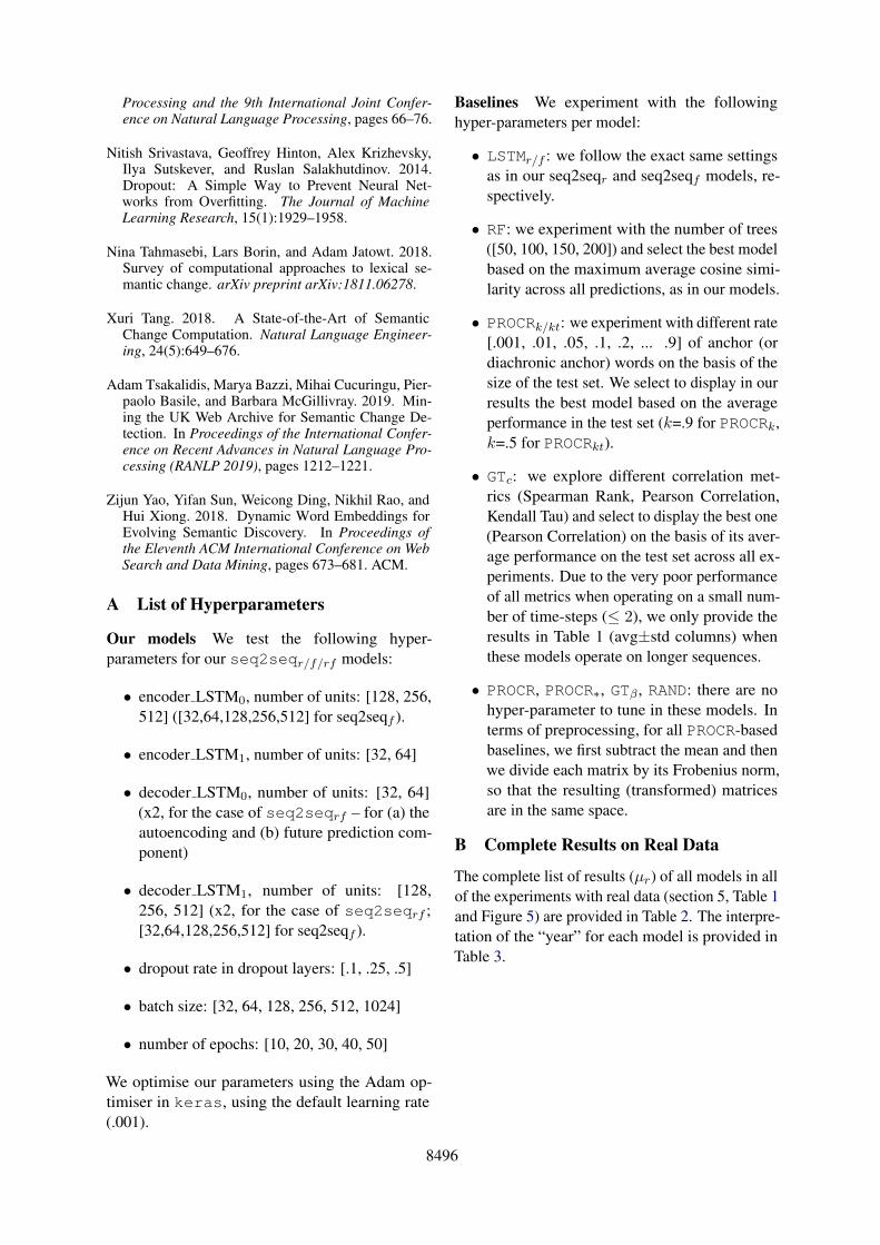
A List of Hyperparameters

Our models We test the following hyper-parameters for our seq2seqr/f/rf models:

• encoder LSTM0, number of units: [128, 256,512] ([32,64,128,256,512] for seq2seqf ).

• encoder LSTM1, number of units: [32, 64]

• decoder LSTM0, number of units: [32, 64](x2, for the case of seq2seqrf – for (a) theautoencoding and (b) future prediction com-ponent)

• decoder LSTM1, number of units: [128,256, 512] (x2, for the case of seq2seqrf ;[32,64,128,256,512] for seq2seqf ).

• dropout rate in dropout layers: [.1, .25, .5]

• batch size: [32, 64, 128, 256, 512, 1024]

• number of epochs: [10, 20, 30, 40, 50]

We optimise our parameters using the Adam op-timiser in keras, using the default learning rate(.001).

Baselines We experiment with the followinghyper-parameters per model:

• LSTMr/f : we follow the exact same settingsas in our seq2seqr and seq2seqf models, re-spectively.

• RF: we experiment with the number of trees([50, 100, 150, 200]) and select the best modelbased on the maximum average cosine simi-larity across all predictions, as in our models.

• PROCRk/kt: we experiment with different rate[.001, .01, .05, .1, .2, ... .9] of anchor (ordiachronic anchor) words on the basis of thesize of the test set. We select to display in ourresults the best model based on the averageperformance in the test set (k=.9 for PROCRk,k=.5 for PROCRkt).

• GTc: we explore different correlation met-rics (Spearman Rank, Pearson Correlation,Kendall Tau) and select to display the best one(Pearson Correlation) on the basis of its aver-age performance on the test set across all ex-periments. Due to the very poor performanceof all metrics when operating on a small num-ber of time-steps (≤ 2), we only provide theresults in Table 1 (avg±std columns) whenthese models operate on longer sequences.

• PROCR, PROCR∗, GTβ , RAND: there are nohyper-parameter to tune in these models. Interms of preprocessing, for all PROCR-basedbaselines, we first subtract the mean and thenwe divide each matrix by its Frobenius norm,so that the resulting (transformed) matricesare in the same space.

B Complete Results on Real Data

The complete list of results (µr) of all models in allof the experiments with real data (section 5, Table 1and Figure 5) are provided in Table 2. The interpre-tation of the “year” for each model is provided inTable 3.

8497

year PROCR PROCRk PROCRkt RF LSTMr LSTMf GTβ GTc PROCR∗ seq2seqr seq2seqf seq2seqrf2000 - - - - - - - - - - 23.86 -2001 34.26 34.54 34.43 37.35 33.67 36.43 - - 34.26 33.66 23.52 23.672002 32.70 32.64 32.41 34.94 31.20 32.98 - - 32.98 34.06 23.39 23.422003 29.24 29.56 29.41 36.94 30.32 32.57 37.59 43.34 31.02 32.44 23.84 23.472004 25.46 25.35 25.03 27.25 24.66 26.08 35.43 42.98 28.68 30.01 24.21 23.502005 29.04 29.40 28.65 31.43 28.98 29.17 38.47 44.47 28.23 29.05 24.77 23.932006 27.73 27.89 27.38 28.86 26.61 26.55 38.74 44.45 27.71 28.58 25.62 24.282007 26.70 26.75 26.64 30.16 25.45 26.39 34.16 41.93 26.98 28.09 26.53 25.172008 28.30 28.34 27.87 32.77 26.25 27.86 35.02 42.86 26.72 27.38 27.30 24.442009 26.10 26.04 25.81 23.27 24.97 23.73 34.23 43.24 26.15 25.71 29.50 24.722010 27.95 27.96 27.38 28.25 28.18 28.19 36.04 44.77 25.81 25.84 30.91 24.832011 25.71 25.85 25.74 28.15 26.07 26.24 34.78 43.99 25.31 24.65 33.65 25.142012 26.77 27.34 27.44 26.51 27.52 27.12 35.18 44.53 24.94 24.42 36.09 24.932013 30.63 31.01 31.91 30.01 27.87 28.62 38.09 47.87 25.01 24.75 - -

AVERAGE 28.51 28.67 28.47 30.45 27.83 28.61 36.16 44.04 27.99 28.36 27.17 24.29

Table 2: Complete µr scores across all runs.

Model Explanation Example (year=2006)PROCRPROCRkPROCRkt

Date to use for aligning the wordvectors with their correspondingones in the year 2000.

The model aligns the word vectors in the year2006 with the word vectors in the year 2000.

LSTMr

The date indicating the word vectors toreconstruct, along with those in the firsttime-step.

LSTMr receives as input the word vectors in theyears 2000 and 2006 and reconstructs them.

LSTMf ,RF

The date indicating the word vectors topredict.

LSTMf /RF receives the word vectors in the year2000 & predicts the word vectors in the year 2006.

PROCR∗,GTc,GTβ

Cut-off date to use for constructingthe time series of the cosine distances.

The time series of cosine distances of every wordare constructed based on the years [2000-2006].

seq2seqrCut-off date in the input, indicatingthe range of years to reconstruct.

seq2seqr is fed with the word representationsin the years [2000-2006] and reconstructs them.

seq2seqfCut-off date in the input, affectingthe range of years to predict.

seq2seqf predicts the word vectors during theyears [2007-2013], given the vectors during theyears [2000-2006] as input.

seq2seqrfCut-off date in the input, indicatingthe range of years to reconstruct &affecting the range of dates to predict.

seq2seqrf receives the word vectors during theyears [2000-2006] and (a) reconstructs them & (b)predicts their representations in [2007-2013].

Table 3: Explanation of the variable “year” in Table 2.