Modelling formation and evolution of transverse dune fields

Jae Hwan Lee1, A. O. Sousa1, E. J. R. Parteli1 and H. J. Herrmann1,2

1Institut fur Computerphysik, Universitat Stuttgart, 70569 Stuttgart, Germany and

2Departamento de Fısica, Universidade Federal do Ceara, 60455-970, Fortaleza, CE, Brazil

(Dated: February 1, 2006)

We model formation and evolution of transverse dune fields. In the model, only

the cross section of the dune is simulated. The only physical variable of relevance is

the dune height, from which the dune width and velocity are determined, as well as

phenomenological rules for interaction between two dunes of different heights. We

find that dune fields with no sand on the ground between dunes are unstable, i.e.

small dunes leave the higher ones behind. We then introduce a saturation length

to simulate transverse dunes on a sand bed and show that this leads to stable dune

fields with regular spacing and dune heights. Finally, we show that our model can be

used to simulate coastal dune fields if a constant sand influx is considered, where the

dune height increases with the distance from the beach, reaching a constant value.

Keywords: Dunes, transverse dune fields, pattern formation, computer simulation.

I. INTRODUCTION

Sand dunes develop wherever sand is exposed to a medium which lifts grains from the

ground and entrains them into saltating flow, where grains impacting onto the sand bed eject

more and more sand until saturation of the wind is reached leading to a stationary flux. The

diverse conditions of wind and sand supply in different regions give rise to a large variety of

dune shapes. After the pioneering work by Bagnold [1], dune morphology and dynamics have

been investigated many times by geologists and geographers [2–11]. For nearly four decades,

they have mainly reported field observations about the conditions under which the different

kinds of dunes appear as well as measured their velocity, their shape, the patterns they

form, the size distribution of sand grains, and many other properties. However, describing

the formation and evolution of a dune field requires knowledge of parameters related to the

geological history of the area, which is in almost all cases not easy to determine. Strong

2

variations in sand supply, climate, wind behavior, and characteristics of the soil over periods

of thousands of years are decisive for the actual pattern of the dune fields observed.

Almost half of all terrestrial sand seas are covered with transverse dunes [1, 6]. These

dunes appear when unidirectional winds act on areas covered with sand, leading to instabil-

ities of the sand bed [12], or for instance when barchan dunes touch at their horns forming

barchanoids [6] and, for increasing amount of sand, giving rise to almost continuous linear

chains propagating in the wind direction [13]. In fig. 1 we show the sketch of a barchan

dune (top) and an image of the dune field “Lencois Maranhenses” (northeastern Brazil), at

its very beginning region, ilustrating a typical situation where an increasing amount of sand

yields the transition barchanoids → transverse dunes (bottom).

The mechanisms responsible for transverse dune formation have been extensively inves-

tigated by physicists and mathematicians from a theoretical point of view [12, 14, 15]. It

has been verified through simulations using a numerical model in three dimensions that an

open system of transverse dunes seems to approach lateral translational invariance under

unidirectional winds [12], allowing modelling transverse dunes in two dimensions. In spite of

the great theoretical advances, many questions concerning the physics of these dunes remain

open, mainly those related to dune interactions in a field and the difficulty in simulating

such systems − real transverse dune fields may reach lengths of hundreds of kilometers.

A simple model to study transverse dune fields has been recently introduced [16]. This

model is defined in terms of the dune height only, from which sand transport, dune velocity

and the field evolution are determined through a set of three phenomenological equations.

The initial conditions consisted of a field of dunes with different heights and spacing, and

the model reproduced the observation that in many fields all transverse dunes have similar

heights. In the present work, we study a different scenario, in which the model is used to

describe the formation of a dune field. Such scenarios can be found for instance in coastal

areas, where the sand is transported by the wind from the sea into the continent, after being

deposited by ocean tides on the beach (fig. 1).

Furthermore, we take into account data of recently performed field measurements for the

aspect ratio of dunes and for inter-dune distances [13], which are related to the recirculating

flow at the lee side (side of the slip face, where avalanches occur) of the dunes and to the

saturation length of the saltating grains [17]. Recently, Besler [18] proposed that dunes

may present solitary wave behavior, an effect which has been investigated in simulations

3

wind

windward side brink

slip-face

horns

FIG. 1: Top: Sketch of a barchan dune. Bottom: In the beginning of the dune field known

as “Lencois Maranhenses”, northeastern Brazil, transverse dunes are formed from the collapse of

barchan dunes and extend over more than 20 km downwind. The orientation of the barchanoids

indicates the average direction of the wind. Image credit to Embrapa Monitoramento por Satelite,

May/1999.

with three-dimensional barchans [19, 20], and with transverse dunes in two dimensions [12].

We define dune interaction according to coalescence and solitary wave behavior, where we

use relations found for interactions of barchan dunes [20], since it has been shown that the

central transverse profile of symmetric barchans may be a good approximation for the height

profile of transverse dunes [17].

4

Our results show that the evolution of dune fields depends strongly on the presence of

a sand bed in the field. If there is no sand between dunes, the dune field presents small

dunes at its end, which wander with high velocity and increase continuously the size of the

field. On the other hand, if the dune field evolves on a sand sheet over which the sand flux

is saturated, the smaller dunes do not wander away, and a regular dune spacing is obtained.

In this case, we find that the time evolution of the dune spacing in the field agrees well with

the results obtained by Werner and Kocurek [21] using a two-dimensional model based on

defect dynamics in transverse bedforms. The number of dunes in the field as a function

of time is also studied and found to decrease quite regularly in time due to coalescence of

dunes. Finally, we use our model to simulate coastal dune fields assuming a constant sand

influx downwind.

The model details are presented in the next section. In section 3 our results are presented

and discussed. Conclusions are made in section 4.

II. MODEL DESCRIPTION

������������������������������������������������������������������������������������������������������������������������������������������������������������������������������������������������������������������������������������������

������������������������������������������������������������������������������������������������������������������������������������������������������������������������������������������������������������������������������������������

windH

r H2r H1dRr h2r h1

h

FIG. 2: Schematic representations of the situation of two transverse dunes.

In our model, the variable which determines the field dynamics is the dune height. Trans-

verse dunes move in the x (wind) direction with a velocity v ≡ dx/dt inversely proportional

to the height h at their crest:

v =a

h, (1)

where a is a phenomenological constant which contains information about wind speed, grain

size, etc. [16]. A geometrical description of the main elements of our model is shown in fig. 2,

where two dunes of heights h and H , H > h, have their profiles represented by triangles.

The dune width L is related to its height h as L = (r1 +r2)h, where r1 = 10 and r2 = 1.5 are

constants determined, respectively, by measurements of the height profile at the windward

5

side of transverse dunes in the field [13] and by the fact that the slip face defines an angle

of approximately 34◦ with the horizontal [1]. The region of recirculating flow at the lee side

of the dune, also called “separation bubble”, has been found to extend downwind from the

brink (which in our model coincides with the crest) up to a distance of the order of 2 − 4

times the dune height [13]. Here, we use a separation bubble of length 4h, thus the quantity

R in fig. 2 has length 4h − r2h = 2.5h for all dunes. The separation bubble of the dunes

has an important implication in interactions of closely spaced dunes, since the net sand flux

inside the bubble is zero [17]. The distance measured from the reattachment point of the

separation bubble of dune i to the foot of the windward side of the next dune downwind,

i + 1, is called here d.

Dune interaction is defined for the case in which a small dune moving in wind direction

behind a larger one eventually reaches, due to its higher velocity, the position of the larger

one. In our model, this event is assumed to occur whenever the separation bubble of dune

i “touches” the windward side of the downwind dune i + 1, or in other words, when d < 0

in fig. 2. It has been found from 3d simulations using a saltation model that barchan dunes

may behave as solitary waves [20], if their sizes are not too different. The idea is that the

interacting dunes exchange sand, the dune downwind decreases in size giving sand to the

smaller dune upwind, and they essentially interchange their roles, like if the smaller dune

would cross the larger one. However, if the faster dune is significantly smaller than the

higher dune downwind, coalescence occurs: The small dune bumps into the larger one and

gets “swallowed up” [19, 20]. In our model, dune interaction is defined according to the

parameter γ: If the ratio of the dune volumes (Vh/VH)initial

= (h/H)2initial

is smaller than γ,

then the dunes coalesce, and the final dune has height hc =√

h2 + H2 [16]; the number of

dunes in the field decreases by unity whenever two dunes coalesce. On the other hand, if

(h/H)2initial

> γ, then solitary wave behavior occurs: dunes interchange their roles and the

relation between their initial and final heights is as follows [20]:

(

h2

H2

)

final

= C

√

(

h2

H2

)

initial

− γ, (2)

obeying the following mass conservation equation:

(h2 + H2)initial = (h2 + H2)final. (3)

Equation (2) is a simplified approximation of the phenomenological observation reported by

6

Duran et. al. [20] for interactions between barchans, where it is shown that (Vh/VH)final

∝exp {−0.22/[(Vh/VH)

initial− const.]}. Although this has been obtained for barchans, we

apply the approach (2) to transverse dunes since careful analysis of 3d simulation results

for the shear stress on barchan dunes have shown that the central cut of these dunes may

be a good description for the height profile of transverse dunes [17]. While in reference [20]

the value of γ that fits the observations for barchans is around 0.15, in the present work we

consider γ as a model parameter to study interaction of transverse dunes in the field. The

value of the constant C in eq. (2) is determined from a fit to the data by Duran et. al.

using the value γ = 0.15, and is found to be C ≈ 1.3. We thus identify two limit cases of

the parameter γ: When γ → 0, no coalescence occurs, and the number of dunes in the field

remains constant, while for γ → 1 every collision of two dunes results in coalescence and the

consequent decrease in the number of dunes in the field. The relations (2) and (3) are two

independent equations that are used to determine the final dune heights after each iteration

in which dunes interact like solitary waves.

As mentioned before, the initial condition in all simulations consists of an empty field (i.e.

without any dune). Afterwards, transverse dunes with random heights of values uniformly

distributed between ha and hb are injected into the field at a constant rate 1/∆t from the

origin x = 0 downwind, moving with velocity v(h) given by Eq. (1). The time interval ∆t

may vary between 1 and 100 time steps. Typical values of dune heights in the beginning of a

dune field are observed to be around 1m. Thus, to study formation of transverse dune fields,

hb will be set close to ha = 1m. However, in cases (i) and (ii) we will use larger values for hb,

thus providing a wider spectrum of dune heights in order to study the effect of coalescence

and solitary wave behavior in the evolution of a dune field. In our simulations, each time

step is defined as 0.01 year. Thus, after each iteration dunes move a distance downwind

given by (0.01 × a)/h m, and may interact with each other according to the rules mentioned

before. The typical simulation time for 10000 iterations is a few tens of seconds running on

a Pentium IV.

Following the dynamics described above, we study three cases: (i) Dunes are injected into

a field with no sand on the ground; (ii) Dune fields are studied when the ground is covered

with a sand bed, where a phenomenological parameter, the saturation length of the saltation

sheet, is introduced. (iii) Finally, we add to case (ii) a differential equation to simulate a

sand influx, which changes the heights of the dunes over the field evolution.

7

III. RESULTS AND DISCUSSION

In cases (i) and (ii) we investigate the evolution of the field due only to interactions of

dunes through coalescence and solitary wave behavior, according to relations (2) and (3),

which are the mechanisms leading to changes in the heights of the dunes. In this case, the

mean dune height in the field doesn’t go beyond the maximum height hb of the injected

dunes.

Figure 3 shows the snapshot of a transverse dune field at t = 104 time steps (100 years)

for case (i) when 100 dunes are injected into the field at regular time intervals ∆t = 0.01

year, using a = 100 m2/year, hb = 10m, and γ = 0.234. Each vertical line segment in this

plot corresponds to the height at the crest of a single dune. Notice that hb = 10m is a

1000 2000 3000 4000x (m)

0

5

10

h (m

)

0 20 40 60 80 100

t (years)

0

10

20

30

40

50

λ (m

)

FIG. 3: The main plot shows the profile of a simulated dune field after t = 100 years, obtained after

input of 100 dunes from wind direction. Dune crests are represented by the vertical line segments.

The dashed line represents the curve h = 104/x. Model parameters are a = 100 m2/year, ∆t = 0.01

year and γ = 0.234. The inset shows the average dune spacing, representing λ ≃ 0.46 t.

8

value quite unrealistic to study the origin of a dune field where dunes are injected from the

beach. However, as mentioned above, we are in this first part of our work only interested in

studying the effect of interactions between dunes during the field evolution. Figure 3 shows

that the initial number of dunes has been reduced by coalescence. Furthermore, we can

see that the height of the dunes in the field decreases as the inverse of the dune position

downwind: The smaller dunes are found at the end of the field. The dashed line in the

main plot represents the curve h = 104/x. The prefactor A of the curve h(x) = A/x is time

dependent, and may be determined from Eq. (1), which leads to h(x) = at/x. The reason

for this behavior is that small dunes bump into larger ones giving rise to the large height

profile at the beginning of the field, while dunes interacting like solitary waves contribute to

the emergence of the small dune heights observed at larger values of x, and the consequent

temporal increase of the field length, i.e. the distance between the dunes at both extremities

of the field. We have also observed that the curve h(x) = A/x is independent of the value of

γ. The inset of fig. 3 shows that the mean spacing λ between the dunes increases indefinitely

with time, since the small dunes at the end of the field, due to their higher velocities, get

more and more apart from the larger ones. Notice that the average dune spacing λ for one

particular realization of transverse dune field may be written as a linear function of the time

t with coefficient in terms of the heights of the first and last dunes, h1 and hN , respectively,

as well as of the total number of dunes in the field, N :

λ =a

N − 1

(

1

hN

− 1

h1

)

t. (4)

For the dune field shown in fig. 3, we have N = 61, h1 = 2.6m and h2 = 9.7m, then we

find that the coefficient of Eq. (4) is approximately 0.46, which agrees with the slope of the

curve shown in the inset of this figure.

In summary, our findings for case (i) show transverse dune fields with decreasing dune

heights with distance and an increasing dune spacing with time, since the smaller faster

dunes wander at the end of the field. However, field measurements [22] have shown that

dune spacing increases with the dune height, as opposed to the situation found in fig. 3,

where spacing between smaller dunes is mostly larger than for higher dunes. Furthermore,

one relevant aspect to be noticed in the dune field of fig. 3 is the quite irregular dune spacing,

where “clusters” of dunes are even observed, which are not found in real transverse dune

fields.

9

An important difference between transverse dune fields observed on terrestrial sand seas

and the dune fields simulated so far using our model lies in the availability of sand on

the ground. In dune fields where transverse dunes appear on a sand sheet over which the

sand flux between the dunes is saturated, regular spacing and similar dune heights are

observed [13]. This happens because the availability of sand yields a saturated flux between

dunes. Saturation is reached within a time interval of a few seconds, and is associated with

the saturation length ls, which is found to decrease with the strength of the wind [17]. In

a transverse dune field developed on a sand bed, this length may be measured from the

reattachment point of the separation bubble of the upwind dune (see fig. 2), where the wind

strength increases from zero (value of the wind strength in the separation bubble) and sand

transport initiates [17]. When the flux becomes saturated, i.e. after a distance d = ls from

the reattachment point, sand is deposited at the foot of the windward side where the wind

strength decreases, and the surface at the beginning of the downwind dune is not eroded.

It follows that no dune can move faster than its upwind neighbor.

To simulate such dune fields, we introduce in our model the phenomenological constant

ls by fixing for the quantity d in fig. 2 a maximum value dmax = ls. We set ls = 2 m. As a

consequence, the maximum crest-to-crest distance in the field, Dcc, is calculated as:

Dcc = r2h + R + ls + r1H, (5)

according to the definitions in fig. 2. It is important to notice that the maximum spacing

Dcc in the field, as predicted by Eq. (5), is not a constant, but does depend on the dune

size, and is larger in dune fields of higher dunes.

Figure 4 shows two simulated dune fields when the saturation length ls is taken into

account (case (ii)). The profile shown in fig. 4(a) corresponds to t = 90 years, where dunes

of initial heights between ha = 1m and hb = 2m have been injected into the field (now a

ground covered with sand) using ∆t = 0.1 year, a = 150 m2/year and γ = 0.3. As we can see

in this figure, all transverse dunes reach approximately the same height, around 1.6m, and

present a quite regular spacing. Figure 4(b) shows another dune field obtained at t = 500

years with ha = 1m and hb = 10m, ∆t = 0.1 year, a = 150 m2/year and γ = 0.3, where

we find dunes regularly spaced and of heights around 8m. As we can see, the value of the

final dune height depends on the initial values of ha and hb. Moreover, comparison of fig. 4

with fig. 3 shows that the introduction of the saturation length leads to much more stable

10

2 4 6 8 10x (km)

0

5

10h (m

)

5 6 7 80

1

2 (a)

(b)

FIG. 4: Transverse dune field obtained when the saturation length ls of the saltation sheet is

considered. Model parameters are ∆t = 0.1 year, a = 150 m2/year, γ = 0.30, and (a) t = 90 years

(b) t = 500 years. The heights of the 100 injected dunes at t = 0 are random numbers between 1

and (a) 2m, (b) 10 m. We see that the two fields present a quite regular dune spacing.

transverse dune fields, since the smaller dunes wandering fast at the end of the field are now

not found anymore.

The time evolution of the number of dunes in the field is shown in fig. 5 for three different

values of the parameter γ, using again ∆t = 0.1 year and a = 300 m2/year. As we can see

in this figure, after injection of the 100 dunes into the field (at t = 10 years as indicated by

the dashed line), the number of dunes decreases quite regularly in time, as also found by

Schwammle et. al. [12] from a two-dimensional model of transverse dune fields. Further-

more, after a certain time, when dunes reach the same height, the number of dunes gets

constant, Nf . In fig. 6, we present the final number of dunes Nf as a function of γ, averaged

over 1000 realizations, when hb = 2m (circles) and hb = 10m (squares), using ha = 1m,

∆t = 0.1 year and a = 300m2/year. As we can see in this figure, for small values of γ

(γ → 0), the number of dunes remains at the initial value N = 100, since coalescence occurs

less frequently. In particular, this effect is more visible when hb = 2 m (circles), because

11

0 20 40 60 80 100t (years)

0

5

10

15

20

25

30

N(t

)

FIG. 5: Number of dunes in the field, N(t), as a function of time t for γ = 0.34, 0.35 and 0.36

(from top to bottom) averaged over 1000 realizations. The dashed line indicates the time when

input of the 100 injected dunes with random heights between 1 and 2 meters finishes. ∆t = 0.1

year and a = 300 m2/year.

in this case dunes have more similar initial heights (between 1m and 2m), and coalescence

between dunes occurs even more rarely. As the value of γ increases, Nf decreases because

dunes coalesce more often in the field; for large values of γ, as discussed before, Nf is equal

to 1. One aspect of particular interest in fig. 6 is that Nf decreases quite suddenly with γ if

the initial heights of the dunes are very similar (curve represented by circles). In particular,

we have found that as hb → ha = 1m, Nf decreases rapidly to unity at γ ≈ 0.30. On the

other side, for a wider range of heights of the injected dunes (hb ≫ ha), Nf decreases more

smoothly with γ, since in this case even small values of γ are large enough for coalescence

to occur.

Figure 7 shows the average dune spacing λ as a function of time using ∆t = 0.1 year,

a = 100 m2/year, γ = 0.3, and considering the saturation length ls = 2m. As we can see

from comparison of this figure with the inset of fig. 3, the inter-dune distances evolve in

12

0 0.1 0.2 0.3 0.4 0.5γ

0

20

40

60

80

100

Nf

FIG. 6: Final number of dunes Nf as a function of γ, averaged over 1000 realizations. The heights

of the 100 injected dunes are random numbers between 1 m and hb, where hb = 2 m (circles) and 10

m (squares). The number of dunes decreases in time due to coalescence between dunes. ∆t = 0.1

year and a = 300 m2/year.

time in a very different way as compared to the case where the saturation length ls was not

taken into account. Figure 7 shows that the dune spacing now increases until it reaches a

saturation value, which corresponds to the equilibrium state of the field, where dunes have

similar heights as shown in fig. 4.

A very similar result was found recently by Werner and Kocurek [21] using a transverse

dune model in two dimensions based on defect dynamics. They found that λ increases

logarithmically in an intermediate time interval until getting constant, as observed in fig. 7.

Their model consists of a set of differential equations to describe the dynamics of the endlines

of two-dimensional transverse dunes (length and width). In their model, which was used

to predict ages of real dune fields [21], interaction between dunes led to a decrease in the

number of defects in the field. We would like to remark that, although fig. 7 suggests that

λ(t) increases approximately with log(t) for 8 ≤ t ≤ 40, we could not find more than one

13

10−1

100

101

102

t (years)

0

10

20

30

λ (m

)

FIG. 7: Mean dune spacing λ as a function of time, averaged over 1000 realizations of dune fields

using γ = 0.3, a = 100 m2/year and ∆t = 0.1 year, after injection of the 300 dunes, which have

initial random heights between 1 m and hb = 2 m. Computational time is 300 minutes on a

Pentium IV computer to obtain this figure.

decade of this possible logarithmic behavior of dune spacing in time.

It is important to notice that the model defined in case (ii) in the absence of any sand

influx reproduced formation of dune fields of regular spacing, just by injection of dunes

downwind onto an empty ground, which interact by coalescence or solitary wave behavior

according to relations (2) and (3). This situation has to be differentiated from the case

studied in ref. [16], where a constant sand influx is considered, and a field of transverse

dunes of random initial heights evolves in time until a constant final height is reached,

which is proportional to the sand influx. There, a regular spacing was only found in the case

where the initial dune spacing and heights were considered to be also regular. Of course, a

serious limitation of our model so far is that the final height of the dunes is limited according

to their initial values.

14

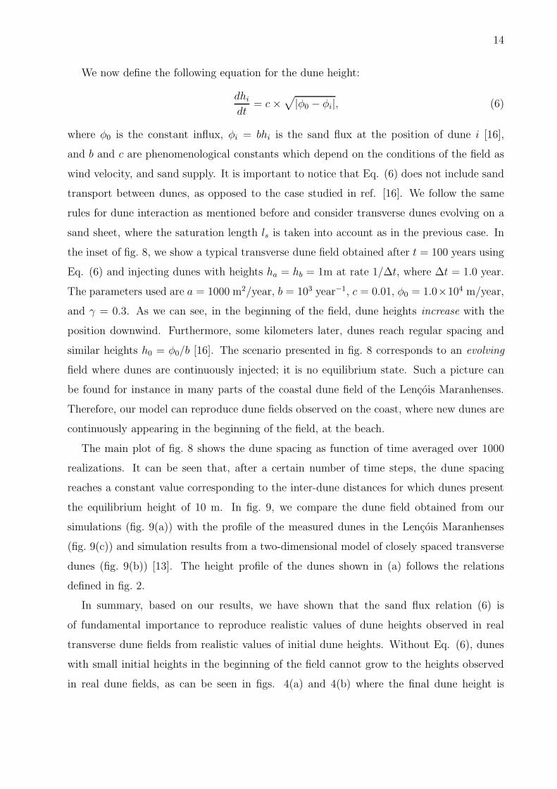
We now define the following equation for the dune height:

dhi

dt= c ×

√

|φ0 − φi|, (6)

where φ0 is the constant influx, φi = bhi is the sand flux at the position of dune i [16],

and b and c are phenomenological constants which depend on the conditions of the field as

wind velocity, and sand supply. It is important to notice that Eq. (6) does not include sand

transport between dunes, as opposed to the case studied in ref. [16]. We follow the same

rules for dune interaction as mentioned before and consider transverse dunes evolving on a

sand sheet, where the saturation length ls is taken into account as in the previous case. In

the inset of fig. 8, we show a typical transverse dune field obtained after t = 100 years using

Eq. (6) and injecting dunes with heights ha = hb = 1m at rate 1/∆t, where ∆t = 1.0 year.

The parameters used are a = 1000 m2/year, b = 103 year−1, c = 0.01, φ0 = 1.0×104 m/year,

and γ = 0.3. As we can see, in the beginning of the field, dune heights increase with the

position downwind. Furthermore, some kilometers later, dunes reach regular spacing and

similar heights h0 = φ0/b [16]. The scenario presented in fig. 8 corresponds to an evolving

field where dunes are continuously injected; it is no equilibrium state. Such a picture can

be found for instance in many parts of the coastal dune field of the Lencois Maranhenses.

Therefore, our model can reproduce dune fields observed on the coast, where new dunes are

continuously appearing in the beginning of the field, at the beach.

The main plot of fig. 8 shows the dune spacing as function of time averaged over 1000

realizations. It can be seen that, after a certain number of time steps, the dune spacing

reaches a constant value corresponding to the inter-dune distances for which dunes present

the equilibrium height of 10 m. In fig. 9, we compare the dune field obtained from our

simulations (fig. 9(a)) with the profile of the measured dunes in the Lencois Maranhenses

(fig. 9(c)) and simulation results from a two-dimensional model of closely spaced transverse

dunes (fig. 9(b)) [13]. The height profile of the dunes shown in (a) follows the relations

defined in fig. 2.

In summary, based on our results, we have shown that the sand flux relation (6) is

of fundamental importance to reproduce realistic values of dune heights observed in real

transverse dune fields from realistic values of initial dune heights. Without Eq. (6), dunes

with small initial heights in the beginning of the field cannot grow to the heights observed

in real dune fields, as can be seen in figs. 4(a) and 4(b) where the final dune height is

15

0 20 40 60 80 100t (years)

0

200

400

600

800

1000λ

(m)

0 2 4 6

x (km)

0

5

10

h (m

)

FIG. 8: The inset shows a simulated dune field after t = 100 years, using the constant influx

according to Eq. (6). Model parameters are a = 1000 m2/year, b = 103 year−1, c = 0.01,

φ0 = 1.0 × 104 m/year, γ = 0.3 and ∆t = 1.0 year. The main plot shows the dune spacing λ as a

function of time averaged over 1000 realizations.

always around hb. Another aspect to be mentioned is the calculation of the parameter γ for

transverse dunes. Due to the great simplicity of our model, no conclusion could be made

about a single threshold value γ = γtransverse which would describe interactions of transverse

dunes, as done recently for barchans in 3 dimensions, where γbarchan ≈ 0.15 [20]. To this

point, simulations of transverse dunes in two dimensions would be required. It would be

also interesting to check if the results found in figs. 6, 7 and 8 may be found from other

numerical models of transverse dune fields in two and/or three dimensions.

16

0 200 400 6000

10

20h

(m) Wind (b)

Wind

0 200 400 600

x (m)

0

10

20 Wind (c)

0 200 400 6000

10

20 (a)

FIG. 9: In (a) we show a typical dune field obtained with our model where the saturation length

ls is considered, with a = 300 m2/year, ∆t = 0.1 year and γ = 0.3, N = 100 injected dunes

and t = 1000 years. (b) and (c) are figures of reference [13]; they are respectively a simulation

of transverse dunes in two-dimensions and the measured profile of a transverse dune field in the

Lencois Maranhenses (fig. 1).

IV. CONCLUSIONS

We presented a simple model to study formation of transverse dune fields. The model

was used to simulate the evolution of dune fields where neighboring dunes may coalesce

or exhibit solitary wave behavior according to their relative volumes. We introduced a

phenomenological parameter, γ, which was compared to the ratio h2/H2 of the volumes

of the interacting dunes of heights h and H , h < H, where coalescence and solitary wave

behavior were defined respectively for h2/H2 < γ and h2/H2 > γ. We found that this

simple rule led to a strong dependence of the field evolution on γ. We have shown that dune

fields formed by input of dunes onto an empty field with no sand on the ground present

decreasing dune heights and increasing spacing with the distance downwind, and the length

of the field increases indefinitely with time. On the other hand, we found that the dune

height and spacing reach an equilibrium value if the saturation length ls of the saltation sheet

17

is considered, where we simulated transverse dune fields evolving on a sand bed. However,

the final dune heights were limited due to the absence of a sand influx. By introducing a sand

influx, we could simulate coastal dune fields with crescent dune heights with distance. We

have shown that, in spite of the simplicity of the model, our results agree with predictions

of simulations from more complex dune models in two dimensions and reproduce well real

transverse dune fields.

Acknowledgments

We acknowledge O. Duran for very important suggestions and discussions, and V. Schatz

for a critical reading of this manuscript. This work was supported in part by the Max-

Plank Price awarded to H. J. Herrmann (2002). E. J. R. Parteli acknowledges support from

CAPES - Brasılia/Brazil.

[1] R. A. Bagnold, The Physics of Blown Sand and Desert Dunes (Methuen, London, 1941).

[2] H. J. Finkel, J. Geol. 67 (1959) 614.

[3] S. Hastenrath, Zeitschrift fur Geomorphologie 11 (1967) 300, and 31-2 (1987) 167.

[4] K. Lettau and H. Lettau, Zeitschrift fur Geomorphologie N. F. 13-2 (1969) 182.

[5] J. T. Long and R. P. Sharp, Geological Society of America Bulletin 75 (1964) 149.

[6] N. Lancaster, Geomorphology of Desert Dunes, Routledge, London, 1995.

[7] K. Pye and H. Tsoar, Aeolian sand and sand dunes, Unwin Hyman, London, 1990.

[8] P. Hesp, Geomorphology 48 (2002) 245.

[9] G. F. S. Wiggs, Progress in Physical Geography 25 (2001) 53.

[10] L. M. Barbosa and J. M. L. Dominguez, Earth Surface Processes and Landforms 29 (2004)

443.

[11] M. G. Kleinhans, A. W. E. Wilbers, A. de Swaaf and J. H. van den Berg, Journal of Sedi-

mentary Research 72 (2002) 629.

[12] V. Schwammle and H. J. Herrmann, Earth Surf. Process. Landforms 29 (2004) 769.

[13] E. J. R. Parteli, V. Schwammle, H. J. Herrmann, L. H. U. Monteiro, and L. P. Maia, Geo-

morphology, in print. cond-mat/0410178.

18

[14] H. Momiji, R. Carretero-Gonzalez, S. R. Bishop, and A. Warren, Earth Surf. Process. Land-

forms 25 (2000) 905.

[15] B. Andreotti, P. Claudin and S. Douady, Eur. Phys. J. B 28 (2002) 341.

[16] E. J. R. Parteli and H. J. Herrmann, Physica A 327 (2003) 554.

[17] G. Sauermann, Modelling of Wind Blown Sand and Desert Dunes, Ph.D. Thesis (Universitat

Stuttgart), Logos Verlag Berlin (2001).

[18] H. Besler, Z. Geomorphol. N. F. 126 (2002) 59.

[19] V. Schwammle and H. J. Herrmann, Nature 426 (2003) 619.

[20] O. Duran, V. Schwammle, and H. J. Herrmann, Phys. Rev. E 72, 021308 (2005). cond-

mat/0406392.

[21] B. T. Werner and G. Kocurek, Geology 27 (1999) 727.

[22] N. Lancaster, Controls of dune morphology in the Namib sand sea. Eolian Sediments and

Processes. M. E. Brookfield and T. S. Ahlbrand Eds., Elsevier (1983) 261.