Sensitivity of Convection-Allowing Forecasts to Land Surface ModelPerturbations and Implications for Ensemble Design

JEFFREY D. DUDA AND XUGUANG WANG

School of Meteorology, University of Oklahoma, Norman, Oklahoma

MING XUE

School of Meteorology, and Center for Analysis and Prediction of Storms, University of Oklahoma,

Norman, Oklahoma

(Manuscript received 9 September 2016, in final form 6 January 2017)

ABSTRACT

In this exploratory study, a series of perturbations to the land surfacemodel (LSM) component of theWeather

Research and Forecasting (WRF) Model was developed to investigate the sensitivity of forecasts of severe

thunderstorms and heavy precipitation at 4-km grid spacing and whether such perturbations could improve

ensemble forecasts at this scale. The perturbations (generated using a combination of perturbing fixed param-

eters and using separate schemes, one of which—Noah-MP—is new among the WRF modeling community)

were applied to a 10-member ensemble including other mixed physics parameterizations and compared against

an identically configured ensemble that did not include the LSM perturbations to determine their impact on

probabilistic forecasts. A third ensemble using only the LSM perturbations was also configured.

The results from 14 (in total) 36-h ensemble forecasts suggested the LSM perturbations resulted in sys-

tematic improvement in ensemble dispersion and error characteristics. Lower-tropospheric temperature,

moisture, and wind fields were all improved, as were probabilistic precipitation forecasts. Biases were not

systematically altered, although some outlier members are present. Examination of near-surface temperature

and mixing ratio fields, surface energy fluxes, and soil fields revealed tendencies caused by certain pertur-

bations. A case study featuring tornadic supercells illustrated the physical causes of some of these tendencies.

The results of this study suggest LSM perturbations can sample a dimension of model error not yet sampled

systematically in most ensembles and should be included in convection-allowing ensembles.

1. Introduction

The state of the land surface and associated surface–

atmosphere exchange processes exert a strong degree of

control over the spatial and temporal patterns of deep

moist convection over land, which draws much of its

energy from the land surface (e.g., Anthes 1984; Rabin

et al. 1990; Clark and Arritt 1995; Pielke 2001; Segele

et al. 2005). Additionally, a correct specification of the

land surface conditions (i.e., the greenness vegetation

fraction, leaf area index, soil texture, and land use) is

critical for accurately forecasting deepmoist convection,

especially during the warm season when the ground

surface is exposed and vegetation is photosynthetically

active (Kurkowski et al. 2003; Robock et al. 2003;

Godfrey et al. 2005; Miller et al. 2006). Therefore, cor-

rect representation of surface–atmosphere exchange

processes in land surface models (LSM) coupled to nu-

merical weather prediction (NWP) models is impor-

tant for accurate forecasts of thunderstorms and heavy

precipitation.

Much of the prior research on the sensitivity of fore-

casts of deep moist convection to surface–atmosphere

exchange processes has indicated that the initial soil

moisture state exerts the most influence. Sutton et al.

(2006), for example, showed that the amount of diversity

in convection-permitting forecasts of precipitation due

to use of different initial soil moisture analyses can rival

that from using varying convection parameterizations in

coarser simulations. Aligo et al. (2007) illustrated the

level of sensitivity of convective-scale forecasts to soil

moisture perturbations and found some skill in proba-

bilistic precipitation forecasts based on an ensembleCorresponding author e-mail: Jeffrey D. Duda, jeffduda319@

gmail.com

MAY 2017 DUDA ET AL . 2001

DOI: 10.1175/MWR-D-16-0349.1

� 2017 American Meteorological Society. For information regarding reuse of this content and general copyright information, consult the AMS CopyrightPolicy (www.ametsoc.org/PUBSReuseLicenses).

using only those perturbations. Trier et al. (2008) de-

termined that the variation in initial soil moisture state

exerted more influence on forecasts of precipitation

than choice of LSM. Finally, while poor coverage of

observations is a major source of uncertainty in soil

moisture analyses, more dense observations will not

eliminate uncertainty, as soil moisture has been shown

to be highly spatially heterogeneous even within a small

area (Basara 2001).

While the importance of an accurate initial soil

moisture state for convection forecasts is paramount,

there is additional uncertainty in the formulation of

physical processes related to energy fluxes. Chen et al.

(1997) compared various methods for parameterizing

surface sensible heat exchange in the LSM used by the

National Centers for Environmental Prediction (NCEP)

for their operational mesoscale model and noted sensi-

tivity to the formulation of the stability term and the

thermal roughness length in calculating turbulent sen-

sible heat flux. Numerous other studies have also iden-

tified sensitivity of precipitation forecasts to the

specification of an empirical constant used to calculate

the thermal roughness length (Zilitinkevich 1995; Chen

et al. 1997), which is used in the formulation of the ex-

change coefficient in the sensible heat flux calculation

(Marshall et al. 2003; LeMone et al. 2008; Chen et al.

2010; Trier et al. 2004, 2011). These studies have shown

(in addition to sensitivity) that certain values of this

constant may result in better agreement between simu-

lated and observed heat fluxes and better precipitation

verification scores than others. Numerous studies have

also suggested that the computation of latent heat flux

from plant transpiration contains many uncertainties.

Perhaps themost important is the resistance term,whether

stomatal resistance or generic canopy resistance, which

governs how effectively plants release water through their

leaves into the environment and how effectively that water

can be carried out of the canopy and into the lower at-

mosphere (Chen and Dudhia 2001; Jackson et al. 2003;

Godfrey and Stensrud 2010; Kumar et al. 2011). Im-

plementation of a comprehensive set of variations based

on these uncertainties in an ensemble forecast framework

has not been documented.

Among the major physics components in convection-

allowing NWP forecasts, which include cloud micro-

physics, boundary layer, radiation, and LSM, uncertainty

in the latter component remains limited in experimental

convection-allowing ensembles, even those that usemixed

physics [see Clark et al. (2009, 2011); Johnson et al.

(2011a,b); Johnson and Wang (2012); Kong et al. (2007);

and Xue et al. (2008), for examples of experimental

convection-allowing ensemble configurations]. Some ex-

perimental ensembles vary theLSMcomponent using one

of two schemes, the Noah LSM (Chen and Dudhia

2001; Ek et al. 2003) and the Rapid Update Cycle

(RUC) LSM (Smirnova et al. 1997, 2000, 2016), which

is sensible considering these schemes are used opera-

tionally. However, large uncertainties exist within

these and other LSMs that have not been accounted for

in convection-allowing ensembles. In this study, an

effort to sample LSM uncertainty and investigate the

sensitivity of forecasts of convection to perturbations

to LSM-related parameters is documented. The im-

plications of adding such LSM perturbations to other

physics perturbations in convection-allowing ensemble

forecast systems are also discussed.

The remainder of this paper is organized as follows. A

brief exposition on the uncertainties within the LSM

component is given in section 2. The experimental setup

is described in section 3. A statistical analysis of verifi-

cation over many cases is presented in section 4. A case

study illustrating the diversity and sensitivity of forecasts

of deep moist convection to various physics perturba-

tions is detailed in section 5. A summary and conclusions

follow in section 6.

2. Uncertainties in land surface modelparameterizations

In the Weather Research and Forecasting (WRF;

Skamarock et al. 2008) Model, the effects of surface–

atmosphere exchange processes occur through feedback

between the LSM and PBL parameterizations. In par-

ticular, sensible heat flux and moisture flux are passed

from the LSM component to the PBL component. The

LSMs contain many uncertainties. Such uncertainties

include the formulation of energy fluxes, the numerical

methods used to approximate the governing equations

of heat and water transport within the soil, and soil and

vegetation state parameters. This work focuses on the

first source of uncertainty.

a. Sensible heat flux

A general formula for sensible heat flux is

H5 rCpC

h(T

s2T

a) , (1)

where rCp serves to convert between radiative transfer

and kinematic units, Ts represents the surface (skin)

temperature, Ta represents the near-surface tempera-

ture, and Ch is the exchange coefficient, representing a

resistance. The formulation of the exchange coefficient

for heat flux varies among LSMs. Many of these for-

mulations are dependent on the thermal roughness

length, z0h, analogous to the momentum roughness

length associated with the log-wind profile in the

2002 MONTHLY WEATHER REV IEW VOLUME 145

surface layer. Thermal roughness length is effectively

impossible to measure directly and must be estimated.

A number of formulations of z0h have been proposed.

One popular formulation (Zilitinkevich 1995) used in

the NCEP operational North American Mesoscale

Forecast System (NAM) is to assume that z0h is related

to the momentum roughness length z0m by

z0m

z0h

5 exp(kCffiffiffiffiffiffiffiffiffi

Re*p

) , (2)

where k is the von Kármán constant, Re* is the stress

Reynolds number, and C is an empirical parameter

whose value is uncertain. Chen et al. (1997) suggest a

standard value of 0.1, but values ranging from 0.01 to 2

have been documented (Zilitinkevich 1995; Marshall

et al. 2003; Trier et al. 2004, 2011; LeMone et al. 2008,

2010). Varying C with location, based on land cover

and/or soil texture, has also been proposed, but has not

been shown to be clearly superior (Trier et al. 2011).

Still other formulations of C and z0h have been pro-

posed (e.g., Chen and Zhang 2009; Chen et al. 2010).

Accounting for this uncertainty in a convection-

allowing ensemble has not been documented, as ex-

isting research (e.g., Chen et al. 1996; Liang et al. 1996;

Yang et al. 2008; Chen and Zhang 2009; Chen et al.

2010) has focused on comparison of forecast energy

flux to observations at a small number of locations as a

means of implementing improvements to a LSM rather

than documenting uncertainty.

b. Latent heat flux

Latent heat flux can be formulated similarly to sensi-

ble heat flux as

LE5 rLyMC

q(q

y,g2 q

y,a), (3)

whereLy is the latent heat of vaporization;M is moisture

availability or soil moisture stress; qy,g and qy,a re-

present moisture terms at ground level and in the

near-surface atmosphere, respectively; and Cqis the

exchange coefficient. This formula is useful in illus-

trating the underlying physical processes of latent heat

flux, but is not always practical since the term qy,g is

ambiguous. There are methods that approximate this

formula or make assumptions about what qy,g repre-

sents. However, it is more common in contemporary

LSMs to partition the total latent heat flux into three

components: 1) bare soil evaporation, 2) canopy water

evaporation, and 3) plant transpiration. The formula-

tions for these three components are highly varied

among existing LSMs. In addition, the calculation of

the exchange coefficient is very complicated in many

schemes, and there are many different ways to formulate

stomatal resistance and soil moisture stress factors that

control latent heat flux.

3. Experimental setup

Based on the uncertainties within available LSMs in

the WRF, a series of perturbations was developed.

These perturbations were then implemented in a set of

10-member ensembles using the Advanced Research

version of the WRF, version 3.6.1, with 4-km grid

spacing. Four LSMs were used to construct the ensem-

bles. They include the Noah, multiparameterization

Noah (Noah-MP; Niu et al. 2011), RUC, and Pleim–Xiu

(PX; Xiu and Pleim 2001; Gilliam and Pleim 2010)

schemes. Despite somemajor differences in the levels of

complexity and the subsurface soil structure (especially

in the PX LSM), preliminary testing revealed that rea-

sonable forecasts can be made using each of these

schemes.

One perturbation method was to vary C in (2), here-

after CZIL. Ensemble members were generated by

sampling from the following set of values: f0.1, 0.25,0.5g. The perturbations were only applied to members

using the Noah LSM. A second perturbation method-

ology was to use various multiparameterization options

in the Noah-MP scheme (Niu et al. 2011). To date, no

study exists documenting the performance of the Noah-

MP scheme in convection-allowing forecasts, neither

deterministically nor in an ensemble framework by us-

ing different choices of processes. This study offers a first

attempt to document the performance of the Noah-MP

scheme in convection-allowing ensemble forecasts. The

various multiparameterization options do not require

coupling, so ensemble members were generated by

comprehensively sampling from the available options

for each process. There are 18 unique combinations of

these options. Readers are referred to Niu et al. (2011)

for details on specific options. The set of options used

in various ensemblemembers is shown inTable 2.Namelist

options opt_crs, opt_sfc, opt_btr, opt_rad, and opt_tbot

refer to methods used for computing plant stomatal

resistance, the exchange coefficient for heat, a soil

moisture stress factor involved in stomatal resistance,

interaction of solar radiation with the vegetation can-

opy, and heat flux at the bottom of the soil (at 2-m

depth), respectively. The third perturbation strategy was

to use multiple LSMs. The multitude of differences in-

cluding soil structure, soil texture, land use classification,

and formulation of physical processes among the LSMs

provides an excellent opportunity to test the effective-

ness of using a mixture of LSMs in an ensemble con-

figuration. These perturbations are detailed in Tables 1

and 2. To isolate the impacts of the LSM perturbations,

MAY 2017 DUDA ET AL . 2003

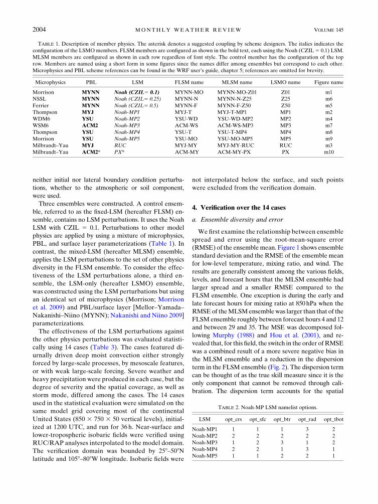
neither initial nor lateral boundary condition perturba-

tions, whether to the atmospheric or soil component,

were used.

Three ensembles were constructed. A control ensem-

ble, referred to as the fixed-LSM (hereafter FLSM) en-

semble, contains no LSM perturbations. It uses the Noah

LSM with CZIL 5 0.1. Perturbations to other model

physics are applied by using a mixture of microphysics,

PBL, and surface layer parameterizations (Table 1). In

contrast, the mixed-LSM (hereafter MLSM) ensemble,

applies the LSM perturbations to the set of other physics

diversity in the FLSM ensemble. To consider the effec-

tiveness of the LSM perturbations alone, a third en-

semble, the LSM-only (hereafter LSMO) ensemble,

was constructed using the LSM perturbations but using

an identical set of microphysics (Morrison; Morrison

et al. 2009) and PBL/surface layer [Mellor–Yamada–

Nakanishi–Niino (MYNN); Nakanishi and Niino 2009]

parameterizations.

The effectiveness of the LSM perturbations against

the other physics perturbations was evaluated statisti-

cally using 14 cases (Table 3). The cases featured di-

urnally driven deep moist convection either strongly

forced by large-scale processes, by mesoscale features,

or with weak large-scale forcing. Severe weather and

heavy precipitation were produced in each case, but the

degree of severity and the spatial coverage, as well as

storm mode, differed among the cases. The 14 cases

used in the statistical evaluation were simulated on the

same model grid covering most of the continental

United States (850 3 750 3 50 vertical levels), initial-

ized at 1200 UTC, and run for 36 h. Near-surface and

lower-tropospheric isobaric fields were verified using

RUC/RAP analyses interpolated to the model domain.

The verification domain was bounded by 258–508Nlatitude and 1058–808W longitude. Isobaric fields were

not interpolated below the surface, and such points

were excluded from the verification domain.

4. Verification over the 14 cases

a. Ensemble diversity and error

We first examine the relationship between ensemble

spread and error using the root-mean-square error

(RMSE) of the ensemblemean. Figure 1 shows ensemble

standard deviation and the RMSE of the ensemble mean

for low-level temperature, mixing ratio, and wind. The

results are generally consistent among the various fields,

levels, and forecast hours that the MLSM ensemble had

larger spread and a smaller RMSE compared to the

FLSM ensemble. One exception is during the early and

late forecast hours for mixing ratio at 850hPa when the

RMSEof theMLSMensemblewas larger than that of the

FLSMensemble roughly between forecast hours 4 and 12

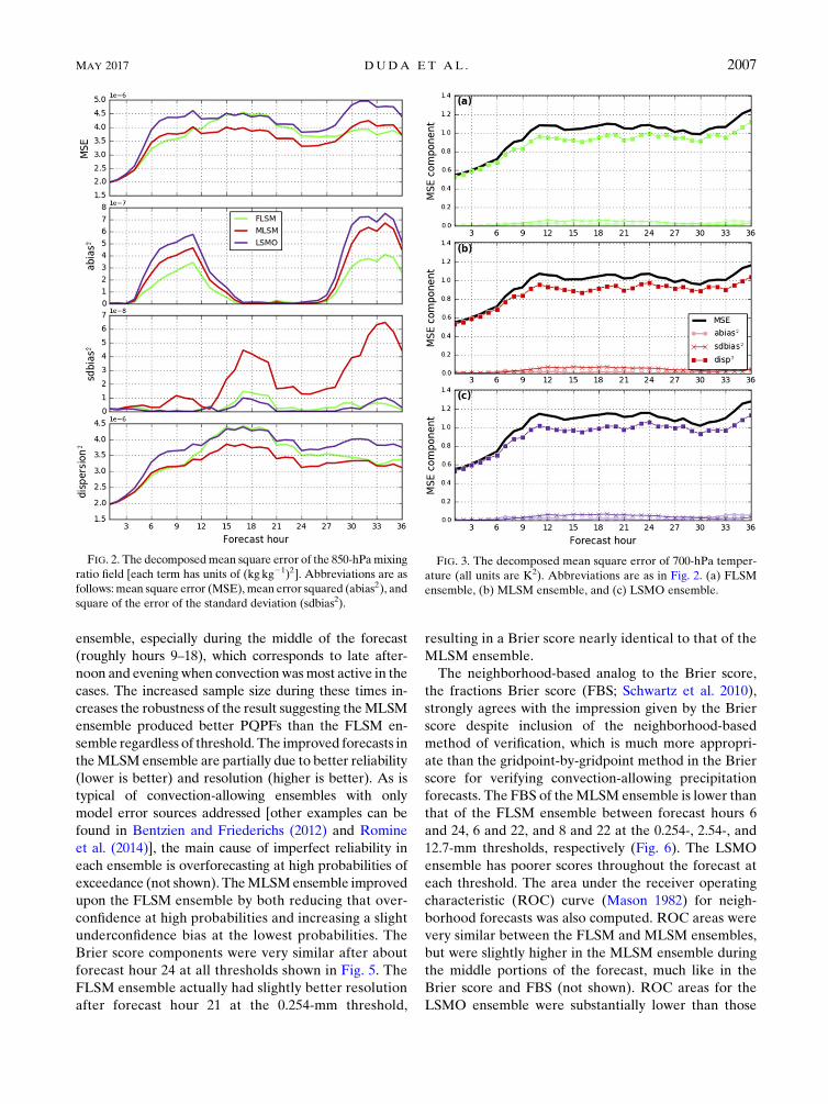
and between 29 and 35. The MSE was decomposed fol-

lowing Murphy (1988) and Hou et al. (2001), and re-

vealed that, for this field, the switch in the order ofRMSE

was a combined result of a more severe negative bias in

the MLSM ensemble and a reduction in the dispersion

term in the FLSM ensemble (Fig. 2). The dispersion term

can be thought of as the true skill measure since it is the

only component that cannot be removed through cali-

bration. The dispersion term accounts for the spatial

TABLE 1. Description of member physics. The asterisk denotes a suggested coupling by scheme designers. The italics indicates the

configuration of the LSMOmembers. FLSMmembers are configured as shown in the bold text, each using the Noah (CZIL5 0.1) LSM.

MLSM members are configured as shown in each row regardless of font style. The control member has the configuration of the top

row. Members are named using a short form in some figures since the names differ among ensembles but correspond to each other.

Microphysics and PBL scheme references can be found in the WRF user’s guide, chapter 5; references are omitted for brevity.

Microphysics PBL LSM FLSM name MLSM name LSMO name Figure name

Morrison MYNN Noah (CZIL5 0.1) MYNN-MO MYNN-MO-Z01 Z01 m1

NSSL MYNN Noah (CZIL5 0.25) MYNN-N MYNN-N-Z25 Z25 m6

Ferrier MYNN Noah (CZIL5 0.5) MYNN-F MYNN-F-Z50 Z50 m5

Thompson MYJ Noah-MP1 MYJ-T MYJ-T-MP1 MP1 m2

WDM6 YSU Noah-MP2 YSU-WD YSU-WD-MP2 MP2 m4

WSM6 ACM2 Noah-MP3 ACM-WS ACM-WS-MP3 MP3 m7

Thompson YSU Noah-MP4 YSU-T YSU-T-MP4 MP4 m8

Morrison YSU Noah-MP5 YSU-MO YSU-MO-MP5 MP5 m9

Milbrandt–Yau MYJ RUC MYJ-MY MYJ-MY-RUC RUC m3

Milbrandt–Yau ACM2* PX* ACM-MY ACM-MY-PX PX m10

TABLE 2. Noah-MP LSM namelist options.

LSM opt_crs opt_sfc opt_btr opt_rad opt_tbot

Noah-MP1 1 1 1 3 2

Noah-MP2 2 2 2 2 2

Noah-MP3 1 2 3 1 2

Noah-MP4 2 2 1 3 1

Noah-MP5 1 1 2 2 1

2004 MONTHLY WEATHER REV IEW VOLUME 145

correlation or phasing error between the forecast and

observed field. The dispersion term contributed more

than 90% of the MSE in the temperature, moisture, and

wind fields (Fig. 3 shows an example for temperature at

700hPa).

The LSMO ensemble contained forecasts that were

competitive with the FLSM and MLSM ensembles

despite the lack of microphysics and PBL diversity.

For example, the LSMO ensemble had a slightly lower

RMSE between forecast hours 12 and 15 in the 925-hPA

y wind, between forecast hours 13 and 15 in the 850-hPa u

wind, and between forecast hours 3 and 8 in the 925-hPa

temperature. In addition, the LSMO ensemble had larger

spread than the FLSM ensemble during the early and late

forecast hours for 925- and 850-hPa temperature (Fig. 1).

These results indicate the value of including LSM per-

turbations to account for model error in an ensemble

approach.

While the macroscopic spread-error statistics of the

MLSM ensemble were improved over the FLSM en-

semble, it is also important to analyze the performance

of individual members within the ensembles. Since each

member uses different physics, each member lies on a

different model attractor, and there may be systematic

bias changes that can reduce the correlation between

ensemble spread and error. It is apparent from Fig. 1

that not only is each ensemble underdispersive (spread

is lower than RMSE throughout the forecast), but that

spread and RMSE do not always evolve together (i.e.,

they are not perfectly correlated). The 850-hPa mean

y-wind error and RMSE for each member of the en-

sembles is shown in Fig. 4. There is more diversity

among the members of the MLSM ensemble than the

FLSM ensemble, a common feature among the fields

verified. However, the LSM perturbations resulted in

some noticeable systematic biases. For example, member

MYJ-MY-RUC of the MLSM ensemble is consistently

negatively biased, and generally has a lower bias than all

other MLSM ensemble members. It also consistently has

the highest RMSE, and so would be regarded as an out-

lier member. There are no outlier members in the FLSM

ensemble. However, there are also several MLSM en-

semble members whose biases are close to 0.0ms21 be-

tween forecast hours 18 and 24 when FLSM ensemble

members are consistently negatively biased. Since the

RMSEs of these members are very similar between en-

sembles during this span, this represents an instancewhen

the MLSM ensemble distribution is truly improved over

the FLSM ensemble.

The y wind at 850hPa was not the only field that ex-

hibited this behavior for member MYJ-MY-RUC. In

fact, this member of the MLSM ensemble had notice-

ably larger RMSEs at nearly every forecast hour in all

wind fields as well as many early forecast hours in the

temperature fields (not shown). Additionally, member

MYNN-N of the FLSM ensemble was an outlier at many

forecast hours in many 925-hPa fields, as was member

MYNN-N-Z50 of the MLSM ensemble. Therefore,

there is some systematic behavior among somemembers

of each ensemble rendering forecast distributions that

are not properly populated. Discounting the outliers in

general, there were fields and forecast hours at which the

distribution of biases and RMSEs in the MLSM en-

semble were more diverse than those of the FLSM en-

semble, indicating a true improvement in the forecast

distribution of the MLSM ensemble over the FLSM

ensemble.

b. Probabilistic precipitation verification

Probabilistic forecasts of 1-h accumulated pre-

cipitation were verified using stage IV precipitation

analyses. Verifying data were mapped to the model grid

using bilinear interpolation. Probabilistic quantitative

precipitation forecasts (PQPFs) were constructed

TABLE 3. List and brief description of the cases used in the statistical analysis.

Date Location of most vigorous convection Main feature(s) of interest

24 May 2011 Central Great Plains Outbreak of supercells and violent tornadoes

14 Apr 2012 Central Great Plains Outbreak of supercells and tornadoes

3 Apr 2014 South-central United States and ‘‘Dixie Alley’’ Large squall line with supercells

27 Apr 2014 Mid-Mississippi Valley Multiple waves of supercells and short squall-line segments

11 May 2014 Central Great Plains Outbreak of mostly nontornadic supercells

3 Jun 2014 Midwest Training supercells and line segments with wind driven large hail

6 Jun 2014 Central high plains Supercells evolving into two MCSs

6 May 2015 Central and southern Great Plains Scattered clusters of tornadic supercells

21 Jun 2015 Northern Great Plains and upper Midwest Fast-moving asymmetric MCS with associated MCV

13 Jul 2015 Great Lakes and mid-Atlantic Multiple squall lines

17 Jul 2015 Northern Great Plains and upper Midwest Supercells evolving into two MCSs

25 Jul 2015 Northern Great Plains and Midwest Marginally severe MCSs

27 Jul 2015 Northern Great Plains Long-lived squall line

28 Jul 2015 Central Great Plains and Midwest Generally nonsevere and disorganized convection along a front

MAY 2017 DUDA ET AL . 2005

using a 50-km circular neighborhood. The results were

fairly similar among various metrics, so only a limited set

are presented. First, the Brier score is shown in Fig. 5,

along with the resolution, reliability, and uncertainty

components. Forecasts in the MLSM and FLSM ensem-

bles were skillful at the lightest threshold (0.254mm)

throughout the forecast, and after forecast hour 12 in the

LSMO ensemble. At the 2.54-mm threshold, the MLSM

ensemble forecasts became skillful at forecast hour 14

while the FLSM and LSMO ensembles followed suit 1

and 4h later, respectively. Forecasts at a high threshold of

12.7mm—a comparatively rare event—were unskillful

throughout the forecast. The Brier score of the MLSM

ensemble was generally lower than that of the FLSM

FIG. 1. Ensemble spread (solid) and RMSE of the ensemble mean (dashed) for the indicated fields, averaged over

the 14 cases.

2006 MONTHLY WEATHER REV IEW VOLUME 145

ensemble, especially during the middle of the forecast

(roughly hours 9–18), which corresponds to late after-

noon and evening when convection wasmost active in the

cases. The increased sample size during these times in-

creases the robustness of the result suggesting theMLSM

ensemble produced better PQPFs than the FLSM en-

semble regardless of threshold. The improved forecasts in

theMLSMensemble are partially due to better reliability

(lower is better) and resolution (higher is better). As is

typical of convection-allowing ensembles with only

model error sources addressed [other examples can be

found in Bentzien and Friederichs (2012) and Romine

et al. (2014)], the main cause of imperfect reliability in

each ensemble is overforecasting at high probabilities of

exceedance (not shown). TheMLSMensemble improved

upon the FLSM ensemble by both reducing that over-

confidence at high probabilities and increasing a slight

underconfidence bias at the lowest probabilities. The

Brier score components were very similar after about

forecast hour 24 at all thresholds shown in Fig. 5. The

FLSM ensemble actually had slightly better resolution

after forecast hour 21 at the 0.254-mm threshold,

resulting in a Brier score nearly identical to that of the

MLSM ensemble.

The neighborhood-based analog to the Brier score,

the fractions Brier score (FBS; Schwartz et al. 2010),

strongly agrees with the impression given by the Brier

score despite inclusion of the neighborhood-based

method of verification, which is much more appropri-

ate than the gridpoint-by-gridpoint method in the Brier

score for verifying convection-allowing precipitation

forecasts. The FBS of theMLSM ensemble is lower than

that of the FLSM ensemble between forecast hours 6

and 24, 6 and 22, and 8 and 22 at the 0.254-, 2.54-, and

12.7-mm thresholds, respectively (Fig. 6). The LSMO

ensemble has poorer scores throughout the forecast at

each threshold. The area under the receiver operating

characteristic (ROC) curve (Mason 1982) for neigh-

borhood forecasts was also computed. ROC areas were

very similar between the FLSM and MLSM ensembles,

but were slightly higher in the MLSM ensemble during

the middle portions of the forecast, much like in the

Brier score and FBS (not shown). ROC areas for the

LSMO ensemble were substantially lower than those

FIG. 2. The decomposedmean square error of the 850-hPamixing

ratio field [each term has units of (kg kg21)2]. Abbreviations are as

follows:mean square error (MSE), mean error squared (abias2), and

square of the error of the standard deviation (sdbias2).

FIG. 3. The decomposed mean square error of 700-hPa temper-

ature (all units are K2). Abbreviations are as in Fig. 2. (a) FLSM

ensemble, (b) MLSM ensemble, and (c) LSMO ensemble.

MAY 2017 DUDA ET AL . 2007

from the FLSM and MLSM ensembles. Thus, the broad

range of verification metrics consistently point to the fact

that the MLSM ensemble produced better probabilistic

forecasts of precipitation than the FLSM ensemble.

c. Land surface properties

1) SURFACE FIELDS

Surface properties like 2-m temperature and mixing

ratio and 10-m wind are highly valuable in assessing the

skill of LSM schemes. However, verification of such

variables was not strictly performed in this study due to the

discovery of problems with some diagnosed fields, espe-

cially 2-m temperature in members using the Noah-MP

LSM. This issue cast considerable doubt on the validity

of verification metrics for these fields. However, a

general sense of the behavior of the members can still

be determined. A physical explanation for the problem

is provided in section 5. Instead of verification, member

mean values of these fields are discussed.

Themean 2-m temperature over the 14 cases is shown in

Fig. 7. The diurnal cycle is clearly evident. Also evident is

the problem with diagnosed 2-m temperature values in

threemembers using theNoah-MPLSM(YSU-WD-MP2,

ACM-WS-MP3, and YSU-T-MP4 in the MLSM ensem-

ble). Daytime temperatures are several degrees warmer

than those in other members. It is also evident that there

is more variability in the 2-m temperature at all forecast

hours in the MLSM ensemble compared to the FLSM

ensemble, even if discounting the three aforementioned

members. Overall the RUC LSM produced cooler tem-

peratures during the daytime and warmer temperatures

at night, while members YSU-WD-MP2/MP2 of the

MLSM/LSMO ensemble were warm during the day and

FIG. 4 (top) Mean errors and (bottom) RMSEs for each member of the (left) FLSM and (right) MLSM

ensembles for 850-hPa y wind (m s21). See Table 1 for the member naming scheme.

2008 MONTHLY WEATHER REV IEW VOLUME 145

coolest at night. There was some tendency for the PX

LSM to produce cooler 2-m temperatures at night.

Issues with diagnosed 2-m mixing ratios are evident

in Fig. 8. Using the values in the FLSM ensemble as a

baseline, there is an anomalous positive bias in mem-

bers using the RUC and Noah-MP LSMs (m3, m4, and

m8, in particular, in the Fig. 8 legend). The bias is es-

pecially notable in the RUC LSM. Considering these

members as outliers and excluding them from the re-

mainder of the analysis, there is not much difference in

the ensemble diversity in the MLSM ensemble com-

pared to the FLSM ensemble, although Fig. 1 suggests

that elsewhere in the troposphere, this is not the case.

Members using the Noah LSM had the lowest 2-m

mixing ratios at all times while the RUCLSM generally

produced the highest mixing ratios. This trend was

evident at higher levels as well (not shown), but less so

with increasing height. Therefore, despite apparent

issues with diagnosed 2-m mixing ratios in the RUC

LSM, it still appears to have produced the highest

overall moisture content. This tendency is consistent

with the surface fluxes.

2) SURFACE ENERGY FLUXES

Time series of average sensible heat flux confirm that

members MYJ-T-MP1 and YSU-MO-MP5 of the

MLSM ensemble and MP1 and MP5 of the LSMO

ensemble produced the highest values during the day-

time, while members MYJ-MY-RUC and YSU-T-MP4

of the MLSM ensemble and RUC and MP4 of the

LSMO ensemble produced the lowest values, although

the tendency was less pronounced during the latter part

of the forecast period in members using the RUC LSM

(not shown). Histograms of sensible heat flux corrob-

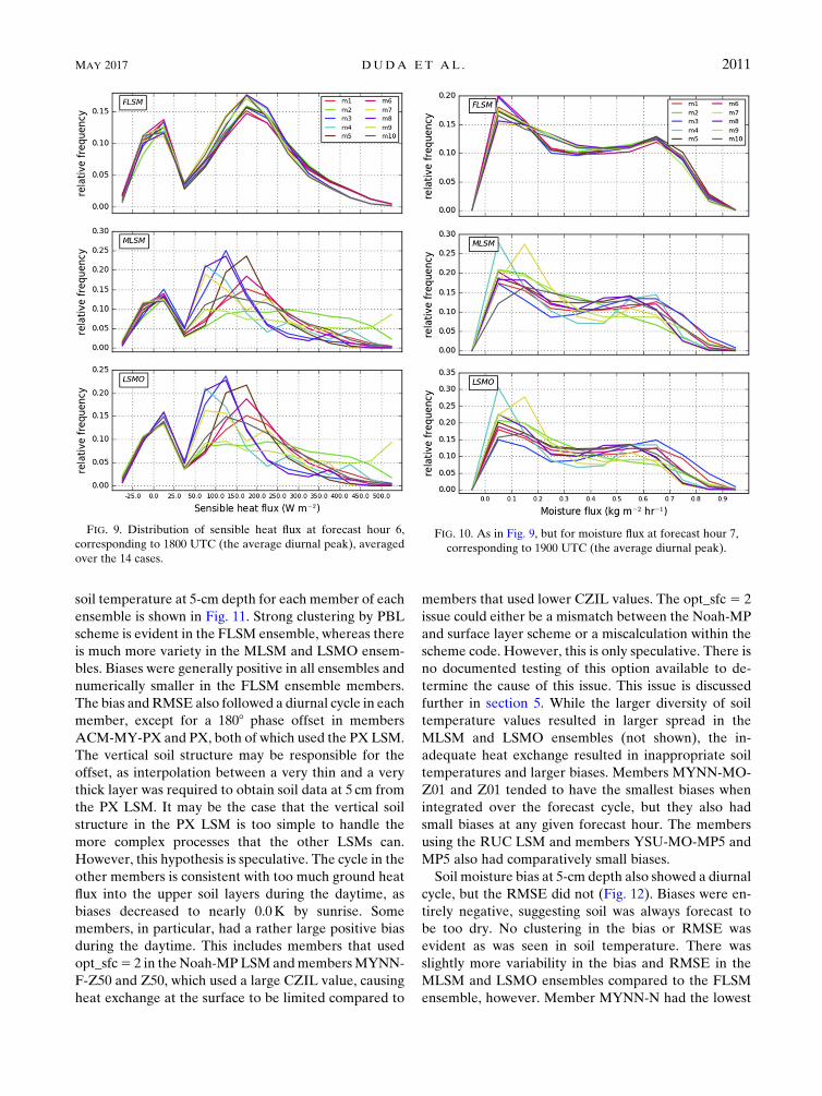
orate these tendencies (Fig. 9). The members with

higher average sensible heat fluxes had flatter, less

modal histograms with a larger fraction of points hav-

ing higher values. In contrast, distributions in members

with the smallest average sensible heat flux values were

not only concentrated in the lower range of the histo-

gram values, but also had left-shifted modes relative to

other members. Unexpectedly, the histogram for

members using the RUC LSM shifted toward higher

values of sensible heat flux on the second day (not

shown), which is unique among the LSMs in this study.

The causes of this are unknown.

FIG. 5. Brier score (thick solid lines) of 1-h accumulated pre-

cipitation at the indicated thresholds. The Brier score components

are also included: reliability (dashed lines with dots), resolution

(dotted lines with 3s), and uncertainty (solid gray).

FIG. 6. Fractions Brier scores for 1-h accumulated precipitation at

the indicated thresholds.

MAY 2017 DUDA ET AL . 2009

Time series of average moisture flux show that

members using the RUC LSM had the largest values

during the daytime compared to other members, al-

though members MYNN-MO-Z01 and ACM-MY-PX

of the MLSM ensemble and Z01 and PX of the LSMO

ensemble also had relatively high values (not shown).

Members using the Noah-MP LSM, especially member

MP3 of the LSMO ensemble, had lower values than

other members, including those established by the Noah

LSM comprising the FLSM ensemble. The distributions

in most members were flat except for a peak at very low

values (Fig. 10). However, members using the RUC

LSM and Noah LSMwith CZIL5 0.1 had more mass at

the upper tail of values, whereas the opposite was true

for members using the Noah-MP LSM.

3) SOIL PROPERTIES

Soil temperature and moisture were verified using

observations from the Oklahoma and west Texas mes-

onets. Verification was limited only to those locations

where valid observations were recorded (i.e., gridded

verification was not performed). A range of 140–150

valid observations per case were used. Verification of

FIG. 7. The 2-m temperature averaged over the 14 cases for each

member of each ensemble.

FIG. 8. As in Fig. 7, but for 2-m mixing ratio.

2010 MONTHLY WEATHER REV IEW VOLUME 145

soil temperature at 5-cm depth for each member of each

ensemble is shown in Fig. 11. Strong clustering by PBL

scheme is evident in the FLSM ensemble, whereas there

is much more variety in the MLSM and LSMO ensem-

bles. Biases were generally positive in all ensembles and

numerically smaller in the FLSM ensemble members.

The bias andRMSE also followed a diurnal cycle in each

member, except for a 1808 phase offset in members

ACM-MY-PX and PX, both of which used the PX LSM.

The vertical soil structure may be responsible for the

offset, as interpolation between a very thin and a very

thick layer was required to obtain soil data at 5 cm from

the PX LSM. It may be the case that the vertical soil

structure in the PX LSM is too simple to handle the

more complex processes that the other LSMs can.

However, this hypothesis is speculative. The cycle in the

other members is consistent with too much ground heat

flux into the upper soil layers during the daytime, as

biases decreased to nearly 0.0K by sunrise. Some

members, in particular, had a rather large positive bias

during the daytime. This includes members that used

opt_sfc5 2 in theNoah-MPLSMandmembersMYNN-

F-Z50 and Z50, which used a large CZIL value, causing

heat exchange at the surface to be limited compared to

members that used lower CZIL values. The opt_sfc 5 2

issue could either be a mismatch between the Noah-MP

and surface layer scheme or a miscalculation within the

scheme code. However, this is only speculative. There is

no documented testing of this option available to de-

termine the cause of this issue. This issue is discussed

further in section 5. While the larger diversity of soil

temperature values resulted in larger spread in the

MLSM and LSMO ensembles (not shown), the in-

adequate heat exchange resulted in inappropriate soil

temperatures and larger biases. Members MYNN-MO-

Z01 and Z01 tended to have the smallest biases when

integrated over the forecast cycle, but they also had

small biases at any given forecast hour. The members

using the RUC LSM and members YSU-MO-MP5 and

MP5 also had comparatively small biases.

Soil moisture bias at 5-cm depth also showed a diurnal

cycle, but the RMSE did not (Fig. 12). Biases were en-

tirely negative, suggesting soil was always forecast to

be too dry. No clustering in the bias or RMSE was

evident as was seen in soil temperature. There was

slightly more variability in the bias and RMSE in the

MLSM and LSMO ensembles compared to the FLSM

ensemble, however. Member MYNN-N had the lowest

FIG. 9. Distribution of sensible heat flux at forecast hour 6,

corresponding to 1800 UTC (the average diurnal peak), averaged

over the 14 cases.

FIG. 10. As in Fig. 9, but for moisture flux at forecast hour 7,

corresponding to 1900 UTC (the average diurnal peak).

MAY 2017 DUDA ET AL . 2011

(most negative) bias and some of the highest RMSEs

among the FLSM ensemble, whereas members MYJ-

T-MP1, YSU-T-MP4, and ACM-MY-PX of the MLSM

ensemble, and members MP1, MP4, and PX of the

LSMO ensemble had the most negative biases and

the largest RMSEs. There is little commonality among

these members to explain this outcome. Members

MYJ-MY-RUC, YSU-WD-MP2, and ACM-WS-MP3

of theMLSM ensemble and RUC,MP2, andMP3 of the

LSMO ensemble had the least negative biases and

lowest RMSEs. This mix of good and bad members

suggests a reasonable set of perturbations was used in

this experiment for forecasts of soil temperature and

moisture.

FIG. 11. (left) Bias and (right) RMSE for soil temperature at 5-cm depth.

2012 MONTHLY WEATHER REV IEW VOLUME 145

5. Case study

Acase study can be valuable in discerning the physical

causes of changes or improvements in the performance

of the MLSM ensemble over the FLSM ensemble. A

case of a severe weather outbreak that occurred on

13 June 2010 is analyzed. This case was not part of the 14

cases used in the systematic evaluation of the ensembles,

but the ensemble members behave in accordance with

the systematic behaviors seen in the evaluation over a

larger number of cases and therefore this case serves as

an excellent example of how LSM perturbations impact

FIG. 12. As in Fig. 11, but for soil moisture at 5-cm depth.

MAY 2017 DUDA ET AL . 2013

the forecast. For brevity, and because the LSM pertur-

bations are isolated in the LSMO ensemble, the dis-

cussion on the physical response of the perturbations

focuses entirely on LSMO ensemble members; the

FLSM and MLSM ensembles are only briefly discussed.

The combination of a high-amplitude trough, un-

seasonably high lower-troposphericmoisture content, and a

climatological triggeringmechanism—a dryline, in this case

accompanied by an outflow boundary (OFB) from a prior

mesoscale convective system (MCS)—provided the neces-

sary ingredients for tornadic supercells in the central plains,

focused across theTexas andOklahomaPanhandles during

the afternoon of 13 June. These cells would later evolve

upscale into an MCS. The case study focuses on the pre-

convective environment during the afternoon preceding

convection initiation as well as initiation itself.

The ensemble precision in initiation location is illus-

trated in Fig. 13. Temporal errors in initiation have been

ignored. An eastward bias is apparent in each ensemble.

However, since every member was 1–3h late in initiation,

the eastward bias may partially be due to advective effects

of the boundary,whichmovedvery slowly eastward in both

the observations and the forecasts during the few-hour

period around initiation. However, examination of near-

surface thermodynamic and forcing fields (not shown)

suggests that even if initiation had occurred on time, dif-

ferences in boundary location and orientation compared to

observations would still have led to errant initiation loca-

tion in most members. Larger variability in the orientation

and placement of the OFB was seen in the FLSM and

MLSM ensembles compared to the LSMO ensemble (not

shown), whereas it is difficult to discern differences in the

variability of the OFB between the FLSM and MLSM

ensembles. In fact, there is little evidence to suggest the

LSM perturbations altered the placement or orientation of

the OFB in any meaningful way prior to initiation. The

choice of PBLormicrophysics schemehadmore impact on

this aspect of the forecast.

Overall, variability in the spatial distribution at initi-

ation was highest in the MLSM ensemble and lowest in

the LSMO ensemble. Whereas each member of the

LSMO ensemble initiated storms within Beaver County,

Oklahoma, and Ochiltree, Lipscomb, Hemphill, and

Roberts Counties, Texas, storms developed in a more

widespread area of the Texas and Oklahoma Panhan-

dles and southwest Kansas in both the FLSM and

MLSM ensembles. There were members that initiated

convection farther northwest and southeast in the

MLSM ensemble compared to the FLSM ensemble.

The PBL across the southern plains during the day-

time of 13 June is now analyzed. Airmass mean energy

fluxes and thermodynamic quantities (potential tempera-

ture and mixing ratio) were calculated for the warm sector

FIG. 13. Paintball plot for composite reflectivity exceeding

40 dBZ for each member of each ensemble (color shades) and

observations (black contour). The forecasts and observations are

staggered in time and show reflectivity approximately 1 h after the

first appearance of reflectivity exceeding 40 dBZ in each member.

The observations are valid at 1900 UTC 13 Jun 2010 while the

forecasts are valid between 2000 and 2200UTC. Counties indicated

in the text are highlighted.

2014 MONTHLY WEATHER REV IEW VOLUME 145

east of the dryline and south of the OFB (containing much

ofOklahomaandTexas) and for the regionbehind (west) of

the dryline (containing mostly west Texas and parts of New

Mexico). Overall, differences among the members in near-

surfacemixing ratio andpotential temperature of 1–2gkg21

and 1–2K, respectively, were common throughout the late

morning and afternoon across Oklahoma and Texas.

Members RUC and PX were noticeably more moist ev-

erywhere (Figs. 14e,f), although the drying west of the

dryline in member RUC was considerably greater than in

any other members, rendering it one of the drier members

by the early evening. Member MP4 was also moist west of

the dryline, but not in the warm sector. MembersMP4 and

PX tended to be cooler with shallower PBLs in both air

masses, and member MP2 was also cool (point soundings

show this better than airmass-averaged quantities; not

shown). Member RUC was cooler in the warm sector, but

warmer behind the dryline, due to an apparent phase offset

in the sensible heat flux pattern (not shown). Members

MP1,MP3, andMP5had thewarmest anddriest, and some

of the deepest, PBLs in the warm sector in the afternoon

(Figs. 14a,c,e). Members with CZIL perturbed were clus-

tered, but member Z01 was warmest west of the dryline

and coolest and themostmoist in thewarm sector, whereas

member Z50 exhibited the opposite trends.

The primary feedback from the LSM component to

the atmospheric component of the WRF occurs through

the sensible heat flux and moisture flux. Since these

processes are bottom boundary forcings for the atmo-

sphere, LSM perturbations should be the most effective

nearest the surface.

Early afternoon sensible heat flux is shown in Fig. 15.

Large differences among the members can be found, es-

pecially in western Texas and eastern NewMexico. In this

area sensible heat flux is the largest in members MP1,

RUC, and MP5. Members MP1 and MP5 use the generic

Monin–Obukhov method (opt_sfc 5 1) in the Noah-MP

LSM (Niu et al. 2011) to calculate the surface exchange

coefficient, and the exchange coefficient for heat is much

larger overmost of the region in thosemembers compared

to most other members, including the other Noah-MP

members (not shown). The higher exchange coefficient

means that for a given temperature difference between the

lowest model level and the ground surface (skin temper-

ature) more heat is transported from the surface into the

atmosphere, which should result in higher near-surface

temperatures and warmer and deeper PBLs. There is

a stark contrast between members MP1 and MP5 and

members MP2, MP3, andMP4, the latter of which use the

Chen et al. (1997) method (opt_sfc 5 2) to calculate the

exchange coefficient. The exchange coefficient in these

latter members is much lower, restricting transport of

heat away from the surface. As a result, there is an

accumulation of heat at the surface, and the energy is in-

stead forced to be transported deeper into the soil, which is

manifest as larger ground heat flux and warmer daytime

soil temperatures (Figs. 16d–f). The opposite is true for

members MP1 and MP5. The very low exchange co-

efficient valuesmay not be reasonable, as further shownby

the diagnosed 2-m temperature over some areas (Fig. 17).

In parts of the mid-South and southeastern United States,

diagnosed 2-m temperature values exceeded 325K during

peak heating! Such values are within a few degrees of

current world record maximum temperatures and are

clearly not legitimate. These temperatures are the result of

the excessive skin temperature from the heat trapped at

the surface. It was this issue that prevented meaningful

verification of 2-m temperature in this study. A similar

issuemay have plagued diagnosed 2-mmixing ratio values

as well, although to a lesser extent.

Sensible heat flux values are also consistent with the

values of CZIL in members Z01, Z25, and Z50. In the

MYNN surface layer scheme, as CZIL increases, z0hdecreases, so the exchange coefficient decreases, as does

sensible heat flux.Member Z50 uses CZIL5 0.5 and has

the smallest sensible heat flux compared to members

Z01 and Z25. Member Z01 uses CZIL5 0.1 and has the

largest sensible heat flux. Because it also has a higher

exchange coefficient, sensible heat flux in member RUC

is among the highest in the LSMO ensemble west of the

dryline. However, east of the dryline, member RUC is

closer to the ensemble mean in terms of sensible heat

flux. As a result, there is less vertical mixing in the PBL

east of the dryline in member RUC, and it remains one

of the cooler and moister members.

Surface moisture flux is of chief importance in driving

variability in moisture content among LSMO members.

Total moisture flux is dependent on many factors, in-

cluding plant type, soil moisture availability, moisture

contrast between the surface and the lower atmosphere,

amount of condensed water present on the vegetation

canopy, and incident solar radiation, but since each LSM

parameterizes moisture flux differently, exchange coeffi-

cients differ strongly among the members. Therefore, dif-

ferences in total moisture flux can arise through a wide

variety of processes. Some processes are discussed below.

Moisture flux accumulated over the daytime of

13 June and prior to initiation is shown in Fig. 18. There

is a large overall increase in moisture flux from west to

east across the region, the result of not only a west–east

increase of soil moisture, but also of an increase in

vegetation density across the region. Across Texas and

western Oklahoma moisture flux is especially larger in

members RUC and PX with more isolated areas of

larger moisture flux in members MP1, MP2, and MP4.

Moisture flux is the lowest in member MP3. The streaky

MAY 2017 DUDA ET AL . 2015

nature of the large moisture flux in member RUC is the

result of large bare soil evaporation (not shown), with

some of the liquid provided by previous overnight con-

vection. On average, however, bare soil evaporation in

member RUC was higher than in any other member

regardless of antecedent soil moisture. While bare soil

evaporation was also high in member PX, plant tran-

spiration drove much of the higher moisture flux in that

member (not shown). The overall low moisture flux in

member MP3 was the result of rather low plant tran-

spiration, unique behavior among members that used

the Noah-MP scheme. There were large differences in

FIG. 14. Airmass-averaged (a),(b) PBL height; (c),(d) potential temperature; and (e),(f) water vapor mixing ratio

(a),(c),(e) east of the dryline and (b),(d),(f) behind the dryline for LSMO ensemble members.

2016 MONTHLY WEATHER REV IEW VOLUME 145

the spatial patterns of both ground evaporation1 and es-

pecially plant transpiration among Noah-MP members,

suggesting an effective perturbation strategy by varying

opt_crs, opt_btr, and opt_rad, all of which should influ-

ence these processes.

A detailed examination of the moisture flux behaviors

in the LSMOensemblemembers is offered using Fig. 19,

taken from a point near the Oklahoma Mesonet site at

Chandler. There is a significant clustering of total

FIG. 15. Sensible heat flux (Wm22) at 1900 UTC 13 Jun 2010 in the LSMO ensemble.

1 Because of the semi-tiling approach in theNoah-MPLSM, bare

soil evaporation is only one component of the full moisture flux

from ground evaporation.

MAY 2017 DUDA ET AL . 2017

surface moisture flux: members using the Noah scheme

and the RUC and PX schemes have the most moisture

flux during the daytime, whereas members using the

Noah-MP scheme have much less moisture flux. Since

there was very little precipitation during the simulation

at this location, there was correspondingly little canopy

water evaporation, so ground evaporation and plant

transpiration provided effectively all of the total mois-

ture flux. The overall large bare soil evaporation in

members RUC and PX is apparent, likely influenced by

larger exchange coefficients in those members com-

pared to those for ground evaporation in the Noah-MP

FIG. 16. Terms in the surface heat budget from LSMO ensemble members: (a) sensible heat flux (Wm22),

(b) difference between skin temperature and temperature at the first model level (K), (c) exchange coefficient for

heat (unitless), soil temperature at (d) 5- and (f) 20-cm depth, and (e) ground heat flux (Wm22). The location is at

(lat, lon) 5 (33.1688N, 100.5688W), corresponding to the west Texas mesonet site near Jayton, TX (KJTS). Soil

temperature observations are included in (d) and (f).

2018 MONTHLY WEATHER REV IEW VOLUME 145

members (not shown). Most of the total moisture flux

was due to plant transpiration in the Noah members,

while the PX LSM also calculated very large plant

transpiration. The soil moisture tendency in the PX

scheme is likely a result of the soil structure. It uses only

two layers to 1-m depth, shallower than the other

schemes. Thus, it is presumably easier for moisture to

move into the atmosphere from the deep layer. It should

also be noted that, although the RUC LSM uses the

same soil texture and land-use categories as the Noah

and Noah-MP LSMs, the threshold values of soil pa-

rameters (e.g., wilting, saturation, and soil matric po-

tential parameters) are different in the RUC LSM. An

additional simulation was run by swapping these values

FIG. 17. Diagnosed 2-m temperature (K) from LSMO ensemble members valid at 1900 UTC 13 Jun 2010.

MAY 2017 DUDA ET AL . 2019

from those used in the Noah scheme to determine if

these parameter differences were the cause of the

greatly different moisture flux behavior in member

RUC. Only minor changes to moisture flux were noted

in the additional run, suggesting that is not the cause.

In two of the Noah-MP members, plant transpiration

decreased to nearly zero during portions of the daytime

(Fig. 19f), caused by stomatal resistance reaching very

large values (not shown) and subsequent very low ex-

change coefficients. In Noah-MP members in which

plant transpiration did not approach zero, stomatal re-

sistance instead became very low during the daytime,

thus the exchange coefficient became large and tran-

spiration proceeded. The behavior of plant transpiration

FIG. 18. Accumulated moisture flux (kgm22) between 1200 and 2000 UTC 13 Jun 2010 from LSMO ensemble

members.

2020 MONTHLY WEATHER REV IEW VOLUME 145

in specific Noah-MP members varied strongly by loca-

tion, however, and only members MP1 and MP5 ex-

hibited similar behavior regardless of location. The

exchange coefficient for transpiration in members Z01,

Z25, Z50, and PX reached similar, but slightly larger,

magnitudes as members MP1 and MP5 during the day-

time (not shown). The resultant transpiration in mem-

bers Z01, Z25, Z50, and PX was thus larger than that in

members using the Noah-MP LSM. The exchange co-

efficient for transpiration was largest in member RUC,

but perhaps due to the difference in formulation of plant

transpiration in the RUC LSM (i.e., the use of a plant

coefficient from a lookup table), transpiration was more

similar to that of the members using the Noah-MP LSM

rather than being overwhelmingly larger than all other

members.

FIG. 19. (a) Surface moisture flux, (b) bare soil evaporation, (d) canopy water evaporation, and (f) plant tran-

spiration (kgm22 s21). Soil moisture at (c) 5- and (e) 25-cm depths from the LSMO ensemble at (lat, lon) 5(36.658N, 96.808W), with observed soil moisture provided by the Oklahoma Mesonet site located near Chandler,

OK. The 1-h accumulated precipitation (mm) is also dotted and scaled to the right-hand vertical axis in (d).

MAY 2017 DUDA ET AL . 2021

In general, the RUC LSM parameterized the largest

bare soil evaporation, although other members, espe-

cially those using the Noah-MP LSM, occasionally had

similar values. Also, the PX LSM parameterized the

largest plant transpiration, although at some locations

members using theNoah LSMand some of themembers

using the Noah-MP LSM had similar or larger values. It

is also worth noting that at locations where no pre-

cipitation was forecast, soil moisture was almost iden-

tical between members, with differences in 5-cm soil

moisture content differing among the members by less

than 1%. However, there were large soil moisture errors.

At the Chandler Mesonet site, for example, there was an

error of around 0.15m3m23 in both 5- and 25-cm soil

moisture in all members except PX, in which the error

was highly variable. However, the soil moisture tendency

forecast was good at the Chandler site, where very little

precipitation was forecast. This was the case at other sites

where soil moisture observations were available as well.

Errors in forecast soil moisture are likely the result of

poor initial soil conditions provided by the 12-km NAM

model analysis.

6. Summary and conclusions

The LSM component contains uncertainties that have

not been sampled in prior experimental storm-scale

ensemble forecast systems. The sensitivity of

convection-permitting (4-km grid spacing) forecasts to

model physics perturbations of theWRFModel, with an

emphasis on perturbations to the LSM component, was

evaluated both qualitatively (using a case study of tor-

nadic supercells and an MCS) and quantitatively

(using a number of cases involving intense deep moist

convection that produced severe weather and heavy

precipitation in the United States). Three ensembles

were configured, each with 10 members, perturbing

different combinations of WRF Model physics compo-

nents. Three methods were used to generate 10 pertur-

bations to the LSM component. One used separate

LSMs that include Noah, Noah-MP, RUC, and PX. The

second method was to alter the namelist options con-

trolling the formulation of various physical processes

within the Noah-MP LSM. The third method was to

perturb CZIL in the Noah LSM. The LSMO ensemble

incorporated these perturbations, but held the micro-

physics and PBL physics fixed. The MLSM ensemble

incorporated the LSM perturbations on top of micro-

physics and PBL physics perturbations. The FLSM en-

semble served as a baseline ensemble that did not

include the LSM perturbations, but did include micro-

physics and PBL perturbations. There were multiple

purposes of conducting this study. One purpose was to

determine if adding LSM perturbations to other physics

perturbations already used in experimental storm-scale

ensembles improved ensemble spread and probabilistic

forecasts. Another purpose was to document the vari-

ability that LSM perturbations alone can generate in a

convective-scale NWP forecast. A third purpose was to

document the performance and behavior of a new LSM,

the multiparameterization-Noah (Noah-MP), which has

not yet been used in experimental warm-season con-

vective-scale forecasts.

Adding LSM perturbations to the FLSM ensemble to

construct the MLSM ensemble had a positive impact on

probabilistic forecasts. Ensemble spread in the MLSM

ensemble was larger than that of the FLSM ensemble for

lower-tropospheric temperature,moisture, and wind, and

theRMSEof the ensemblemeanwas lower in theMLSM

ensemble compared to the FLSM ensemble for those

fields. Verification of PQPFs also suggested a positive

benefit from adding LSM perturbations. Some outlier

behavior was noted in a few members of each ensemble,

where forecasts were consistently poorer than in other

members. The LSMperturbations had some effect on the

systematic biases of the members. This is not necessarily

optimal for improving ensemble design, as an optimal

ensemble should contain unbiased members so that

chaotic error growth dominates over systematic error

growth. Careful consideration should be used to construct

unbiased ensemble members before implementing these

LSM perturbations in an operational setting.

The case study illustrated the impacts that the LSM

perturbations had on the forecasts, mainly through al-

terations of the surface energy fluxes and near-surface

thermodynamic fields. The perturbations also impacted

PBL structure, causing some members to have shal-

lower, cooler, and moister PBLs and others to have

deeper, warmer, and drier PBLs. Also, the LSM per-

turbations increased the spatial variability in the initia-

tion of storms despite a negligible impact on an outflow

boundary, which was critical to the forecast.

The Noah-MP LSM offered a convenient way to

generate ensemble members by changing namelist op-

tions for parameters thought to be important for warm

season forecasts. However, one option for calculating

the surface heat exchange coefficient (opt_sfc 5 2) re-

sulted in unrealistic diagnosed 2-m temperature values.

The temperatures were too warm, the result of excessive

heat storage at the ground surface caused by low ex-

change coefficients. This was an undesirable outcome

for investigating ensemble design, which seeks to ad-

dress uncertainty rather than perturb a value or process

to the point of being unreasonable. This issue does not

appear to have been fixed in recentWRFModel updates

(through version 3.8.1 at the time of writing).

2022 MONTHLY WEATHER REV IEW VOLUME 145

This was an exploratory study on LSM perturbations. It

is not guaranteed that the particular set of perturbations

applied in this study is the best set of perturbations to use.

It is certainly not the only possible set of perturbations.

Future work should consider using other combinations of

namelist options to generate ensemblemembers using the

Noah-MP LSM (18 combinations exist), as well as de-

termine how sensitive each option actually is. Both prior

research and the results herein suggest that convective-

scale forecasts are not as sensitive to handling heat flux at

the bottom of the soil (opt_tbot) as they are to calculating

the surface exchange coefficient (opt_sfc). Finally, it may

be necessary to perturb CZIL over a larger range, as lit-

erature review suggests a wider range of values may be

necessary to capture all variability associated with that

parameter. Itmay also be useful to include othermethods

of calculating the thermal roughness length, some of

which do not include CZIL. The important result from

this work, however, is that adding a reasonable set of

LSM perturbations improves convective-scale ensemble

forecasts.

Acknowledgments. This research was primarily sup-

ported by NSF Grants AGS-1046081 and AGS-0802888

and NOAA Grant NA16OAR3450236. WRF simula-

tions were conducted using the Stampede supercom-

puter at the Texas Advanced Computing Center, with

thanks to the Extreme Science and Engineering Dis-

covery Environment (XSEDE) program, and also using

supercomputing resources provided by theUniversity of

Oklahoma (OU) Supercomputing Center for Education

and Research (OSCER). Some experimental aspects

were inspired by conversations between the lead author

and David Stensrud. This paper was improved from

thoughtful comments from two anonymous reviewers.

REFERENCES

Aligo, E. A., W. A. Gallus, and M. Segal, 2007: Summer rainfall

forecast spread in an ensemble initialized with different soil

moisture analyses.Wea. Forecasting, 22, 299–314, doi:10.1175/

WAF995.1.

Anthes, R. A., 1984: Enhancement of convective precipitation by

mesoscale variations in vegetative covering in semiarid re-

gions. J. Climate Appl. Meteor., 23, 541–554, doi:10.1175/

1520-0450(1984)023,0541:EOCPBM.2.0.CO;2.

Basara, J. B., 2001: The value of point-scale measurements of soil

moisture in planetary boundary layer simulations. Ph.D. dis-

sertation, University of Oklahoma, 225 pp.

Bentzien, S., and P. Friederichs, 2012: Generating and calibrating

probabilistic quantitative precipitation forecasts from the

high-resolution NWP model COSMO-DE. Wea. Forecasting,

27, 988–1002, doi:10.1175/WAF-D-11-00101.1.

Chen, F., and J. Dudhia, 2001: Coupling an advanced land surface-

hydrology model with the Penn State–NCARMM5 modeling

system. Part I: Model implementation and sensitivity. Mon.

Wea. Rev., 129, 569–585, doi:10.1175/1520-0493(2001)129,0569:

CAALSH.2.0.CO;2.

——, and Y. Zhang, 2009: On the coupling strength between the

land surface and the atmosphere: From viewpoint of surface

exchange coefficients. Geophys. Res. Lett., 36, L10404,

doi:10.1029/2009GL037980.

——, and Coauthors, 1996: Modeling of land surface evaporation

by four schemes and comparison with FIFE observations.

J. Geophys. Res., 101, 7251–7268, doi:10.1029/95JD02165.

——, Z. Janjic, and K. Mitchell, 1997: Impact of atmospheric

surface-layer parameterizations in the new land-surface scheme

of the NCEP mesoscale Eta model. Bound.-Layer Meteor., 85,

391–421, doi:10.1023/A:1000531001463.

Chen, Y., K. Yang, D. Zhou, J. Qin, and X. Guo, 2010: Improving

the Noah land surface model in arid regions with an appro-

priate parameterization of the thermal roughness length.

J. Hydrometeor., 11, 995–1006, doi:10.1175/2010JHM1185.1.

Clark, A. J., W. A. Gallus, M. Xue, and F. Kong, 2009: A com-

parison of precipitation forecast skill between small

convection-allowing and large convection-parameterizing

ensembles. Wea. Forecasting, 24, 1121–1140, doi:10.1175/

2009WAF2222222.1.

——, and Coauthors, 2011: Probabilistic precipitation forecast skill

as a function of ensemble size and spatial scale in a convection-

allowing ensemble.Mon.Wea.Rev., 139, 1410–1418, doi:10.1175/

2010MWR3624.1.

Clark, C. A., and R. W. Arritt, 1995: Numerical simulations of the

effect of soil moisture and vegetation cover on the develop-

ment of deep convection. J. Appl. Meteor., 34, 2029–2045,

doi:10.1175/1520-0450(1995)034,2029:NSOTEO.2.0.CO;2.

Ek, M. B., K. E. Mitchell, Y. Lin, E. Rogers, P. Grunmann,

V. Koren, G. Gayno, and J. D. Tarpley, 2003: Implementation

of Noah land surface model advances in the National Centers

for Environmental Prediction operational mesoscale eta

model. J. Geophys. Res., 108, 8851, doi:10.1029/2002JD003296.

Gilliam, R. C., and J. E. Pleim, 2010: Performance assessment of

new land surface and planetary boundary layer physics in the

WRF-ARW. J. Appl.Meteor. Climatol., 49, 760–774, doi:10.1175/

2009JAMC2126.1.

Godfrey, C. M., andD. J. Stensrud, 2010: An empirical latent heat

flux parameterization for the Noah land surface model.

J. Appl. Meteor. Climatol., 49, 1696–1713, doi:10.1175/

2010JAMC2180.1.

——, ——, and L. M. Leslie, 2005: The influence of improved land

surface and soil data on mesoscale model predictions. 19th

Conf. on Hydrology, San Diego, CA, Amer. Meteor. Soc., 4.7.

[Available online at https://ams.confex.com/ams/Annual2005/

webprogram/Paper86050.html.]

Hou, D., E. Kalnay, and K. K. Droegemeier, 2001: Objective ver-

ification of the SAMEX ’98 ensemble forecasts. Mon. Wea.

Rev., 129, 73–91, doi:10.1175/1520-0493(2001)129,0073:

OVOTSE.2.0.CO;2.

Jackson, C., Y. Xia, M. K. Sen, and P. L. Stoffa, 2003: Optimal

parameter and uncertainty estimation of a land surface model:

A case study using data from Cabauw, Netherlands.

J. Geophys. Res., 108, 4583, doi:10.1029/2002JD002991.

Johnson, A., and X. Wang, 2012: Verification and calibration of

neighborhood and object-based probabilistic precipitation fore-

casts from a multimodel convection-allowing ensemble. Mon.

Wea. Rev., 140, 3054–3077, doi:10.1175/MWR-D-11-00356.1.

——, ——, F. Kong, and M. Xue, 2011a: Hierarchical cluster

analysis of a convection-allowing ensemble during the Haz-

ardous Weather Testbed 2009 Spring Experiment. Part I:

MAY 2017 DUDA ET AL . 2023

Development of the object-oriented cluster analysis method

for precipitation fields. Mon. Wea. Rev., 139, 3673–3693,

doi:10.1175/MWR-D-11-00015.1.

——, ——, ——, and ——, 2011b: Hierarchical cluster analysis

of a convection-allowing ensemble during the Spring Ex-

periment of the Hazardous Weather Testbed in 2009.

Part II: Ensemble clustering over the whole experiment

period. Mon. Wea. Rev., 139, 3694–3710, doi:10.1175/

MWR-D-11-00016.1.

Kong, F., and Coauthors, 2007: Preliminary analysis on the real-

time storm-scale ensemble forecasts produced as a part of the

NOAAHazardous Weather Testbed 2007 spring experiment.

22nd Conf. on Weather Analysis and Forecasting /18th Conf.

on Numerical Weather Prediction, Park City, UT, Amer.

Meteor. Soc., 3B.2. [Available online at https://ams.confex.

com/ams/22WAF18NWP/techprogram/paper_124667.htm.]

Kumar, A., F. Chen, D. Niyogi, J. G. Alfieri, M. Ek, andK.Mitchell,

2011: Evaluation of a photosynthesis-based canopy resistance

formulation in the Noah land-surface model. Bound.-Layer

Meteor., 138, 263–284, doi:10.1007/s10546-010-9559-z.

Kurkowski, N. P., D. J. Stensrud, and M. E. Baldwin, 2003: As-

sessment of implementing satellite-derived land cover data in

the Eta model. Wea. Forecasting, 18, 404–416, doi:10.1175/

1520-0434(2003)18,404:AOISDL.2.0.CO;2.

LeMone, M. A., M. Tewari, F. Chen, J. G. Alfieri, and D. Niyogi,

2008: Evaluation of the Noah land surface model using data

from a fair-weather IHOP_2002 day with heterogeneous sur-

face fluxes. Mon. Wea. Rev., 136, 4915–4941, doi:10.1175/

2008MWR2354.1.

——, F. Chen, M. Tewari, J. Dudhia, B. Geerts, Q. Miao, R. L.

Coulter, and R. L. Grossman, 2010: Simulating the IHOP_2002

fair-weather CBL with the WRF-ARW-Noah modeling sys-

tem. Part I: Surface fluxes and CBL structure and evolution

along the eastern track. Mon. Wea. Rev., 138, 722–744,

doi:10.1175/2009MWR3003.1.

Liang, X., E. F. Wood, and P. Lettenmaier, 1996: Surface soil

moisture parameterization of the VIC-2L model: Evaluation

and modification. Global Planet. Change, 13, 195–206,

doi:10.1016/0921-8181(95)00046-1.

Marshall, C. H., K. C. Crawford, K. E. Mitchell, and D. J.

Stensrud, 2003: The impact of the land surface physics in the

operational NCEP Eta model on simulating the diurnal cycle:

Evaluation and testing using Oklahoma Mesonet data. Wea.

Forecasting, 18, 748–768, doi:10.1175/1520-0434(2003)018,0748:

TIOTLS.2.0.CO;2.

Mason, I., 1982: Amodel for assessment of weather forecasts.Aust.

Meteor. Mag., 30, 291–303.Miller, J., M. Barlage, X. Zeng, H. Wei, K. Mitchell, and

D. Tarpley, 2006: Sensitivity of the NCEP/Noah land surface

model to the MODIS green vegetation fraction data set.

Geophys. Res. Lett., 33, L13404, doi:10.1029/2006GL026636.

Morrison, H., G. Thompson, and V. Tatarskii, 2009: Impact of

cloud microphysics on the development of trailing stratiform

precipitation in a simulated squall line: Comparison of one-

and two-moment schemes. Mon. Wea. Rev., 137, 991–1007,

doi:10.1175/2008MWR2556.1.

Murphy, A. H., 1988: Skill scores based on the mean square

error and their relationships to the correlation co-

efficient. Mon. Wea. Rev., 116, 2417–2424, doi:10.1175/

1520-0493(1988)116,2417:SSBOTM.2.0.CO;2.

Nakanishi, M., and H. Niino, 2009: Development of an improved

turbulence closure model for the atmospheric boundary layer.

J. Meteor. Soc. Japan, 87, 895–912, doi:10.2151/jmsj.87.895.

Niu, G.-Y., and Coauthors, 2011: The community Noah land sur-

face model with multiparameterization options (Noah-MP):

1. Model description and evaluation with local-scale mea-

surements. J. Geophys. Res., 116, D12109, doi:10.1029/

2010JD015139.

Pielke, R.A., 2001: Influence of the spatial distribution of vegetation

and soils on the prediction of cumulus convective rainfall. Rev.

Geophys., 39, 151–177, doi:10.1029/1999RG000072.

Rabin, R. M., S. Stadler, P. J. Wetzel, D. J. Stensrud, and

M. Gregory, 1990: Observed effects of landscape variability

on convective clouds. Bull. Amer. Meteor. Soc., 71, 272–280,

doi:10.1175/1520-0477(1990)071,0272:OEOLVO.2.0.CO;2.

Robock, A., and Coauthors, 2003: Evaluation of the North

American Land Data Assimilation System over the southern

Great Plains during the warm season. J. Geophys. Res., 108,

8846, doi:10.1029/2002JD003245.

Romine, G. S., C. S. Schwartz, J. Berner, K. R. Fossell, C. Snyder,

J. L. Anderson, and M. L. Weisman, 2014: Representing fore-

cast error in a convection-permitting ensemble system. Mon.

Wea. Rev., 142, 4519–4541, doi:10.1175/MWR-D-14-00100.1.

Schwartz, C. S., and Coauthors, 2010: Toward improved

convection-allowing ensembles: Model physics sensitivities

and optimizing probabilistic guidance with small ensemble

membership. Wea. Forecasting, 25, 263–280, doi:10.1175/

2009WAF2222267.1.

Segele, Z. T., D. J. Stensrud, I. C. Ratcliffe, and G. M. Henebry,

2005: Influence on a hailstreak on boundary layer evolution.

Mon. Wea. Rev., 133, 942–960, doi:10.1175/MWR2897.1.

Skamarock, W. C., and Coauthors, 2008: A description of the

Advanced Research WRF version 3. NCAR Tech. Note

NCAR/TN-4751STR, 113 pp., doi:10.5065/D68S4MVH.

Smirnova, T. G., J. M. Brown, and S. G. Benjamin, 1997: Perfor-

mance of different soil model configurations in simulating

ground surface temperature and surface fluxes. Mon. Wea.

Rev., 125, 1870–1884, doi:10.1175/1520-0493(1997)125,1870:

PODSMC.2.0.CO;2.

——, ——, ——, and D. Kim, 2000: Parameterization of cold-

season processes in the MAPS land-surface scheme.

J. Geophys. Res., 105, 4077–4086, doi:10.1029/1999JD901047.

——,——,——, and J. S. Kenyon, 2016: Modifications to the Rapid

Update Cycle Land Surface Model (RUC LSM) available in

the Weather Research and Forecasting (WRF) Model. Mon.

Wea. Rev., 144, 1851–1865, doi:10.1175/MWR-D-15-0198.1.

Sutton, C., T.M.Hamill, andT. T.Warner, 2006:Will perturbing soil

moisture improve warm-season ensemble forecasts? A proof of

concept. Mon. Wea. Rev., 134, 3174–3189, doi:10.1175/

MWR3248.1.

Trier, S. B., F. Chen, and K. W. Manning, 2004: A study of con-

vection initiation in a mesoscale model using high-resolution

land surface initiation conditions. Mon. Wea. Rev., 132, 2954–

2976, doi:10.1175/MWR2839.1.

——,——,——,M. A. LeMone, and C. A. Davis, 2008: Sensitivity

of the PBL and precipitation in 12-day simulations of warm-

season convection using different land surface models and soil

wetness conditions. Mon. Wea. Rev., 136, 2321–2343,

doi:10.1175/2007MWR2289.1.

——,M. A. LeMone, F. Chen, and K. W. Manning, 2011: Effects

of surface heat and moisture exchange on ARW-WRF

warm-season precipitation forecasts over the central

United States. Wea. Forecasting, 26, 3–25, doi:10.1175/

2010WAF2222426.1.

Xiu, A., and J. Pleim, 2001: Development of a land surface

model. Part I: Application in a mesoscale meteorological

2024 MONTHLY WEATHER REV IEW VOLUME 145

model. J. Appl. Meteor., 40, 192–209, doi:10.1175/

1520-0450(2001)040,0192:DOALSM.2.0.CO;2.

Xue, M., and Coauthors, 2008: CAPS realtime storm-scale en-

semble and high-resolution forecasts as part of the NOAA

Hazardous Weather Testbed 2008 Spring Experiment. 24th

Conf. on Severe Local Storms, Savannah, GA, Amer. Meteor.

Soc., 12.2. [Available online at http://twister.ou.edu/papers/

Xue_24SLS_conf_2008SpringExperiment.pdf.]

Yang, K., and Coauthors, 2008: Turbulent flux transfer over bare-

soil surfaces: Characteristics and parameterization. J. Appl.

Meteor. Climatol., 47, 276–290, doi:10.1175/2007JAMC1547.1.

Zilitinkevich, S. S., 1995: Non-local turbulent transport: Pollution

dispersion aspects of coherent structure of convective flows.Air

Pollution III—Volume I. Air Pollution Theory and Simulation,

C. A. Brebbia, S. S. Zubir, and A. S. Hassan, Eds., Computa-

tional Mechanics Publications, 53–60.

MAY 2017 DUDA ET AL . 2025