1

Seminar on Economic and Market Analysis for Central and Eastern Seminar on Economic and Market Analysis for Central and Eastern European countries (CEEC) and Baltic StatesEuropean countries (CEEC) and Baltic States

Czech Republic, Prague 9-11 September 2003

2

Fundamentals of Markets Diagram 1

Business DecisionsConsumersdecisions

Supply Demand

Market

3

Why Analytical Tools? qAnalysis of Producers/Business

Behaviour. qAnalysis of Consumers Behaviour. qAnalysis of Environment.qWhy Need for Behavioral Analysis? qPremise: Past behaviour influences

present attitude and provides indicators of future behaviour.

4

Supply Side FunctionalityDiagram 2

Stockholders Management &labour

Physical Assets Human Resource

Objective:Maximize

Profit

BusinessEnterprise

Services Goods&Services

Goods

5

Markets Redefine Objectives Diagram 3

Producer Consumer

Supply

Consumer Surplus

Demand

Produ

cer S

urplu

s

Market Value

6

Key Market Functionality

vDetermines/Assigns value to goods & services. vDetermines/assigns allocation of

resources for production and distribution of goods & services; vDetermines social welfare. vAnalysis of value is critical to market

analysis.

7

Investment vInvestment decision function of expected

return. I = ƒE(V)vInvestment, expected to mature in year n

is normally made in year1.vSo investment decision in year1 is a

function of E(Vn) discounted to its value in year1 (present value (PV))

1.0. PV = p/(1+ i) + p/(1+ i)2……. p/(1+ i)n

vWhere p = expected profit (return) and vi = discount rate and n time period usually

in years.

8

Investment Decision (? )

1.1. ? t = tS1n Rt – Ct

• (1 + i)t

vR = Total revenue vC= Total cost vTotal revenue and total cost expansion:vRt = St * Pt

vCt = Ut * Çt

9

Revenue/Cost Permutations

1.2. ? R = Mr = ?S/? P = (S2 – S1)/S1 = d S• (P2 – P1)/P1 d P1.3. ? C = Mc = ? U/? Ç = (U2 – U1)/U1 = d U• (Ç2 – Ç1)/ Ç1 d ÇvMr = Marginal revenuevMc = Marginal costvd = Partial derivative

10

Variables

vS = Quantity of goods/services sold vP = price, good/service vU = units of goods/services

produced vÇ = unit cost of goods/services

11

Function Slope = dy/dx Diagram 4.

Slope

= dy

/dx =

McCost

Units produced

12

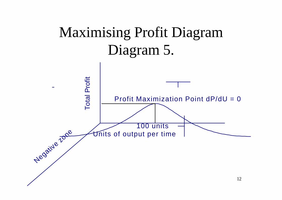
Maximising Profit Diagram Diagram 5.

Negative zo

ne

Tota

l Pro

fit

Units of output per time

Profit Maximization Point dP/dU = 0

100 units

13

Profit Function qLet profit function (P) be expressed as:1.4. P = - $10 000 + $ 400U – 2U2

vWhen output (U) is zero the firm incurs a loss ofv $ 10, 000 vAs output increases profit increases. vProfit is maximised/minimised at the point:vdP/dU = 400 – 4U = 0 v4U = 400vU = 100. vBeyond 100 units profit begins to decline.

14

• To ascertain whether profit is maximised or minimised, take the second derivative:

• d2P• d2U • Point of maximization is where:• d2P is negative and minimization where• d2U it is positive • So where:• dP = 400 – 4U = 400 – 4(100) = 0• dU • d2P = -4 confirms that at output 400 profit is• d2U maximised.

15

Quantitative Analysis of Discount Rate

qInterest is the return on investment. qCorrelation between level of return and

risk qPositive correlation Risk free investment

and low return. 1.5. ? = ƒ(µ)Where:v? = risk; and vµ = uncertainty.

16

Estimating Uncertainty vNo precise estimator.vProbability: likelihood of occurrence of an

event is normally used as an indicator of uncertainty.vAssume there is a 70% chance that per minute

tariff will fall with the introduction of a new mobile operator then: vLikelihood of price fall = 0.7vLikelihood of no price fall = 0.3 vThe sum of probabilities of an event should = 1

17

Application

vAssume company is considering the options of investing $ 1 million in either:

(i) Expansion 2.5G network (ii) Introduction 3G network Assume that both projects are dependent onthe level of domestic economic activity as given at table x.

18

Table x

State of Economy Probability Project 2.5 G Project 3 G Recession 0.2 $ 400 $ 0 Normal 0.6 $ 500 $ 500 Boom 0.2 $ 600 $ 1, 000

19

Expected Profit vExpected profit (Ê(? )) is the weighted average

of profits (? ) in various states of the economy. 1.6. Ê(? ) = i S1

n ? i Pi

vWhere: o P indicates probability and i = 1-n o E.g. the expected profit for the projects at

Table X are:1.7. Ê(? a) = 400(0.2) + 500(0.6) + 600(0.2) = 5001.8. Ê(? b) = 500(0.6) + 1,000(0.2) = 500

20

Range of outcomeDiagram 6

400100100200200

"TheChasm"

Expected profit

Pro

babi

lity

of o

ccur

renc

e

Mean0 200 400 600 1000500

Profit

.02

.04

.06

21

Observations vInverse relationship between probability of

distribution and risk ;vRisk is higher the further the dispersion

from the expected value vRisk is lower when variation of probable

outcome is closer to the expected value vTherefore dispersion around expected value

determines degree of risk.vRange for Project A = 400-600vRange for Project B = 0-1000

22

Estimating Dispersion, (Standard Deviation)

1. Calculate expected value (mean of distribution): Ê? = S? i Pi

2. Calculate deviation from Ê? := ? i - Ê?3.Calculate the variance of probability of

distribution:s 2 = S (? i - ? )2Pi

v Standard Deviation s = (s 2)½

23= 63.25s= 4,000s 2

= 200010,000* 0.210,000600 – 500 = 100

= 0 0* 0.60500 – 500 = 0

= 2,00010,000 * 0.210,000400 – 500= - 100

Coefficient of Variation = s / Ê?

Variance * Probability (? i - ? )2Pi

Variance (? i - ? )2

Deviation(? i - Ê? )

24

Adjusting Market Value for Risk

vRewriting Equation (1.0):1.9. PV = tSn

1 p/(1+ i)t, vRisk adjustment:trade off investors are

likely to make based on the degree of uncertainty. vRisk premium is the difference between

the required rate of return and risk free rate of return on an investment.vRisk adjustment is effected through

changes in the discount rate i

25

Req

uire

d R

ate

of R

etur

n

Risk (Standard Deviation)0 0.5 1.0 1.5

5%

7%

10%

15%

O-5%=Risk freeRate Of Return

>5% - 15% = Risk Premium Range

26

qThe Adjusted Present Value to account for risk (RVP) is :

2.0. RPV = tS18 p/(1+ r)t

Working Example: vProject A : Roll out GSM network in region Y vProject B : Roll out GSM network in region zvInvestment on both projects = $100,000vExpected annual return over 8 yrs

= $ 20,000 (Project A) & $23,000 (Project B)vs for Project A = 1.0 vs for Project B = 1.5 vAdjusted Costs of capital (r) are 10 % project A &

15% Project B.

27

Risk Adjusted Value (RPV)2.2. RPVProject A = 20,000 - 100,000• (1.10)8

= 20,000 *1 - 100,000(1.10)8

= 20,000 x 5.335 – 100,000= 6,700

.

28

Risk Adjusted Value (RPV)

2.3. RPVProject B = 23,000 - 100,000• (1.15)8

= 23,000* 1 - 100,000(1.15)8

= 23,000 x 4.487 -100,000= 3,200

29

Other Risk Assessment Methodologies

qCoefficient of Variation = s / Ê?qBeta method: measures risk for which investors require compensation.

30

Quantitative Analysis, DemandvApplication of Quantitative methods to

study, simulate and forecast consumers response to change in factors that are likely to influence their purchase of a good/service. vA Demand Function may be expressed as: v(Qt) = ƒ tS1

n(x1t, x2t , x3t, ……xnt).vThe fundamental problem is how to

measure the relationship between Qt & SXit.

31

Demand & Profit 2.4. ?pt = ƒ(?Rt – ?Ct) = ƒ[? (Qt* Pt) – ?Ct]qAssuming:

?Qt = ƒ S? (Pt, Yt, At, pt, Tt ….u)Where:P = Price of Q Y= Disposable IncomeA = Direct & indirect advertisementp= price of related goods/services T= taste u= other factors.

32

Sensitivity vProblem:vTo estimate the sensitivity of interrelationship

between:1. (Pt, Yt, At, pt, Tt ….ut) & Qt

2. (Pt, Yt, At, pt, Tt ….ut) & revenue (R) and in turn3. (Pt, Yt, At, pt, Tt ….ut) & the level of profit (p).vSensitivity is normally involves measurement elasticity (?) the multiplier that prescribes the degree of responsiveness of one variable to a changein another variable, ceteris paribus.

33

Methods of Measurement of Elasticity

q? = dQ * X Point elasticity• dX Q

• OrqÉ = dQ * X! Arc elasticity • dX Q!• ! indicates the mean

34

Measuring Demand Sensitivity vAssume that demand (annual) for a service (a) is

expressed in terms of the linear function:2.5. Qa = a1P + a2Y + a3Pop + a4Ic + a5AvWhere vP = Price of avY= Income vPop = Population vIc = Index of credit availability vA = Advertising expenditure va1 – a5 are coefficients of the independent variables.

35

vAssume that the respective coefficients were measured as:v3000 for pricev1,000 for income v0.05 for populationv1, 500,000 for Index of credit availabilityv0.05 for Advertisement.Then:2.6. Qa = - 3000P + 1,000Y + 0.05Pop +

1,5000,000Ic + 0.05A

36

qAssuming that:§ Y = 2,000§ Pop= 200, 000,000§ Ic = 1.0§ A = 100,000,000qIn terms of Price:2.7. Qa = - 3000P + 1,000(2,000) +

0.05(200,000,000) + 1,5000,000(1)+ 0.05(100,000,000)

= 18,500,000 – 3000P

37

Pric

e

Quantity service demanded per year

Average price per T1

6.167

18.5m0

Demand Curve for serviceQ = 18, 500,000 - 3,000PP = 6,167 - .00033Q

38

Pric

e

Quantity of service demanded per year

Average price per unit of service

6.167

18.5m0

Demand Curve for serviceQ = 18, 500,000 - 3,000PP = 6,167 - .00033Q

3.5

3.0

8m 9.5m

39

Point Elasticity

(2.7. Qa = - 3000P + 1,000Y + 0.05Pop + 1,5000,000Ic + 0.05A)

Assume a proposed price increase from 3,000 to 3,500.2.8. dQa .= - 3,000 a constant

dP At:P = 3,000 and Q = 9,500,0002.9. ? = - 3000(3000/9,500,000)

= - 0.95.

40

qAt: P = 3,500 and Q = 8,000,0003.0. ? = -3,000(3,500/8,000,000)

= - 1.3qSo elasticity can change along a demandCurve and could very between:o Inelastico Unitary o Elastic

41

Arc Elasticity

• É = -3,000(3,000 + 3,500)/2______• (8,000,000 + 9,500,000)/2• = 1.114• GENERALLY, NOT MANY

ENTERPRISES HAVE DATA TO CALCULATE POINT ELASTICITIES.

42

Real World Calculation of Decision Parameters

Regression Analysis:qBasically, a combination of mathematical and

statistical methods to estimate values of parameters.qWidely used for:o Simulation exercises; o Forecasting/predicting socio-

economic/financial/market behaviour.

43

Statement ofRelationship to be

investigated

Observation of DataRelationship forspecification ofmathematical

function

Identification/Specification of data

requirement re:dependent &independent

variables

Specification ofEquation/s to

estimate function

Listing of statisticalassumptions for tovalidate estimates

Run regression model

Undertakestatistical tests of

relevantParameters

Interpret Results

Application ofresults for future

estimates

Application ofresults for current

estimates

Application ofresults for

sensitivity analysis

Regression Analysis Module

44

Identification/Specification of Issue

Statement of issue:qE.g. Service provider applies for an increase in

monthly residential telephone access rates in rural area X. qOne of the factors the Regulator and operator

should seek to establish for decision making is the sensitivity of households in area X to changes in telephone access rates.

45

Identification of Demand Function

Identification of critical factors that impact net monthly residential telephone connections (Qt)Given the data at the following table it seems Reasonable to assume that (Qt) is affected by: qMonthly access rate for residential telephone, Pt; qMonthly Disposable income per household,Yt in area X.3.1. Qt = ƒ(Pt ,.Yt)

46

Observed data

6.50501307.15551306.90601157.50601257.15651105.6070807.35701056.3070907.00701007.2080906.3090705.5010055

YPQ

47

100

90

80

70

65

Mon

thly

Acc

ess

Cha

rges

60

55

50

55

Net Monthly Connections

1251151101051009080700

45o L

ine

130

48

Specification of Regression Equation

3.1. Qi = ß1 - ß2 Pi + ß3Yi+ ui

q U is the stochastic term involving thefollowing assumptions:o ui is normally distributedo E(ui) = 0 o E(ui

2) = s 2

o E(uiuj) = 0 o The explanatory variables are non-

stochasticqNote ß1 is the mean of Q when each of the

explanatory variables is equal to zero.

49

Least Sq Estimates of Regression Coefficient

3.2. S = iS113(Qi - ß1 - ß2 Pi - ß3Yi)2

qDifferentiating S with respect to ß1, ß2 and ß3:

3.3. dS = -2 iS(Qi - ß1 - ß2 Pi - ß3Yi)d ß1

3.4. dS = -2 iS Pi(Qi - ß1 - ß2 Pi - ß3Yi)d ß2

3.5. dS = -2 iS Yi(Qi - ß1 - ß2 Pi - ß3Yi)d ß2

50

qMinimizing and rearranging terms:3.6. S Qi = ßn1 + ß2 S Pi + ß3 S Yi

3.7. S Pi Qi = ß1S Pi + ß2 S P2i + ß3 S Pi Yi

3.8. S YiQi = ß1S Yi + ß2 S Pi Yi + ß3 S Y2i

qSo :3.9. ß1 = S Qi/n - ß2 S Pi/n- ß3 S Yi/nqSubstituting ß1 into the normal equations and

converting them into matrix form.

ØNote most regression package would do these iterations.

51

a22 a23

a23 a33

aq2 a23

aq3 a33

a22a23 – a223

aq2a23 -aq3a23

ß2 =

80192250*4.86 –(-54)2

= 10,631.5 = - 1.326-3550*4.86-(-54)* 125.25

80198019= 90,112.5 = 11.2372250 * 125.5- (-54) * -(350)

a22 a23

a23 a33

a22 aq2

a23 aq3

a22a23 – a223

a22aq3a23aq2

ß3 =

52

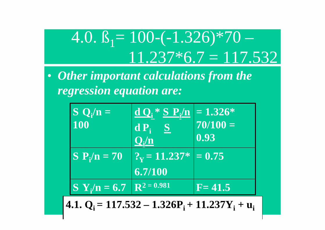
4.0. ß1= 100-(-1.326)*70 –11.237*6.7 = 117.532

• Other important calculations from the regression equation are:

F= 41.5R2 = 0.981S Yi/n = 6.7

= 0.75?Y = 11.237*6.7/100

S Pi/n = 70

= 1.326* 70/100 = 0.93

d Qi * S Pi/nd Pi SQi/n

S Qi/n = 100

4.1. Qi = 117.532 – 1.326Pi + 11.237Yi + ui

53

Statistical Tests

Significant ß2 = 2.41

Significant ß2 = 2.30

Test for multi-collinearity

Significant2.262ß1 = 2. 44t=!ß - ß*sß

Test for auto correlation

Confidence Interval95% two tail test

T values for 13-9 Degrees of Freedom

Estimated t values t equation

54

Annex 1Basics for Optimization

Techniques 1. Y = aXb

dy/dx = baXb-1

2. Y = U*V• dy/dx = V du/ Dx + U dv/dx

• E.g. Y= 3x2(3-x)

• dy/dx = (3-x)(6x) + 3x2(-1)

55

• Y = U/V• dy/dx = V du/dx - U dv/dx

• V2

• Y = 2x – 3• 6x2

• dy/dx = 6x2(2) – (2x – 3)12x• 36x4

• = 3-x• 3x3

56

• Y = 2U – U2

• Where U = 2x3

• dy/dx = dy/du* du/dx =

• dy/du = 2 – 2(2x3)• du/dx = 6x2

• = (2-4x3)6x2

• = 12x2 – 24x5

57

• Second order derivatives:• if du/dx = 2cQ – 3dQ2

• Then:

• du2/dx2 = 2c – 6dQ

58

üY = aebx then dy/dx = baebx

üY = a log bx then dy/dx = a/x

üY = ax then dy/dx = ax log xüY = a sin bX then dy/dx = ab cos bXüY = a cos bX then dy/dx = -ab sin bX