Semantic Segmentation with Boundary Neural Fields

Gedas BertasiusUniversity of Pennsylvaniagberta@seas.upenn.edu

Jianbo ShiUniversity of Pennsylvania

jshi@seas.upenn.edu

Lorenzo TorresaniDartmouth Collegelt@dartmouth.edu

Abstract

The state-of-the-art in semantic segmentation is cur-rently represented by fully convolutional networks (FCNs).However, FCNs use large receptive fields and many pool-ing layers, both of which cause blurring and low spatialresolution in the deep layers. As a result FCNs tend to pro-duce segmentations that are poorly localized around objectboundaries. Prior work has attempted to address this issuein post-processing steps, for example using a color-basedCRF on top of the FCN predictions. However, these ap-proaches require additional parameters and low-level fea-tures that are difficult to tune and integrate into the originalnetwork architecture. Additionally, most CRFs use color-based pixel affinities, which are not well suited for semanticsegmentation and lead to spatially disjoint predictions.

To overcome these problems, we introduce a BoundaryNeural Field (BNF), which is a global energy model inte-grating FCN predictions with boundary cues. The bound-ary information is used to enhance semantic segment co-herence and to improve object localization. Specifically, wefirst show that the convolutional filters of semantic FCNsprovide good features for boundary detection. We then em-ploy the predicted boundaries to define pairwise potentialsin our energy. Finally, we show that our energy decom-poses semantic segmentation into multiple binary problems,which can be relaxed for efficient global optimization. Wereport extensive experiments demonstrating that minimiza-tion of our global boundary-based energy yields results su-perior to prior globalization methods, both quantitativelyas well as qualitatively.

1. IntroductionThe recent introduction of fully convolutional networks

(FCNs) [22] has led to significant quantitative improve-ments on the task of semantic segmentation. However, de-spite their empirical success, FCNs suffer from some limita-tions. Large receptive fields in the convolutional layers andthe presence of pooling layers lead to blurring and segmen-tation predictions at a significantly lower resolution than the

Figure 1: Examples illustrating shortcomings of prior se-mantic segmentation methods: the second column showsresults obtained with a FCN [22], while the third columnshows the output of a Dense-CRF applied to FCN predic-tions [19, 7]. Segments produced by FCN are blob-like andare poorly localized around object boundaries. Dense-CRFproduces spatially disjoint object segments due to the use ofa color-based pixel affinity function that is unable to mea-sure semantic similarity between pixels.

original image. As a result, their predicted segments tend tobe blobby and lack fine object boundary details. We reportin Fig. 1 some examples illustrating typical poor localiza-tion of objects in the outputs of FCNs.

Recently, Chen at al. [7] addressed this issue by apply-ing a Dense-CRF post-processing step [19] on top of coarseFCN segmentations. However, such an approach introducesseveral problems of its own. First, the Dense-CRF adds newparameters that are difficult to tune and integrate into theoriginal network architecture. Additionally, most methodsbased on CRFs or MRFs use low-level pixel affinity func-tions, such as those based on color. These low-level affini-ties often fail to capture semantic relationships between ob-jects and lead to poor segmentation results (see last columnin Fig. 1).

We propose to address these shortcomings by means ofa Boundary Neural Field (BNF), an architecture that em-ploys a single semantic segmentation FCN to predict se-mantic boundaries and then use them to produce semanticsegmentation maps via a global optimization. We demon-strate that even though the semantic segmentation FCN hasnot been optimized to detect boundaries, it provides good

1

...Convolutional Feature Maps

RGB Input ImageSegmentation Mask in Softmax Layer

Minimize Global Energy

Boundaries

|{z}

...wn( )++( )w1

X

i

✓i(zi)+X

ij

✓ij(zi, zj)

Linear Combination of Feature Maps

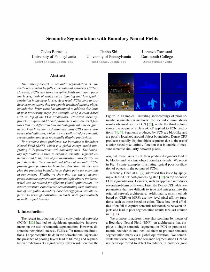
Figure 2: The architecture of our system (best viewed incolor). We employ a semantic segmentation FCN [7] fortwo purposes: 1) to obtain semantic segmentation unariesfor our global energy; 2) to compute object boundaries.Specifically, we define semantic boundaries as a linear com-bination of these feature maps (with a sigmoid function ap-plied on top of the sum) and learn individual weights corre-sponding to each convolutional feature map. We integratethis boundary information in the form of pairwise potentials(pixel affinities) for our energy model.

features for boundary detection. Specifically, the contribu-tions of our work are as follows:

• We show that semantic boundaries can be expressedas a linear combination of interpolated convolutionalfeature maps inside an FCN. We introduce a boundarydetection method that exploits this intuition to predictobject boundaries with accuracy superior to the state-the-of-art.

• We demonstrate that boundary-based pixel affinitiesare better suited for semantic segmentation than thecommonly used color affinity functions.

• Finally, we introduce a new global energy that de-composes semantic segmentation into multiple binaryproblems and relaxes the integrality constraint. Weshow that minimizing our proposed energy yields bet-ter qualitative and quantitative results relative to tradi-tional globalization models such as MRFs or CRFs.

2. Related WorkBoundary Detection. Spectral methods comprise one

of the most prominent categories for boundary detection.In a typical spectral framework, one formulates a general-ized eigenvalue system to solve a low-level pixel grouping

problem. The resulting eigenvectors are then used to pre-dict the boundaries. Some of the most notable approachesin this genre are MCG [2], gPb [1], PMI [17], and Normal-ized Cuts [28]. A weakness of spectral approaches is thatthey tend to be slow as they perform a global inference overthe entire image.

To address this issue, recent approaches cast boundarydetection as a classification problem and predict the bound-aries in a local manner with high efficiency. The most no-table examples in this genre include sketch tokens (ST) [20]and structured edges (SE) [9], which employ fast randomforests. However, many of these methods are based onhand-constructed features, which are difficult to tune.

The issue of hand-constructed features have been re-cently addressed by several approaches based on deep learn-ing, such as N4 fields [11], DeepNet [18], DeepCon-tour [26], DeepEdge [3], HFL [4] and HED [31]. All ofthese methods use CNNs in some way to predict the bound-aries. Whereas DeepNet and DeepContour optimize ordi-nary CNNs to a boundary based optimization criterion fromscratch, DeepEdge and HFL employ pretrained models tocompute boundaries. The most recent of these methods isHED [31], which shows the benefit of deeply supervisedlearning for boundary detection.

In comparison to prior deep learning approaches, ourmethod offers several contributions. First, we exploit the in-herent relationship between boundary detection and seman-tic segmentation to predict semantic boundaries. Specif-ically, we show that even though the semantic FCN hasnot been explicitly trained to predict boundaries, the con-volutional filters inside the FCN provide good features forboundary detection. Additionally, unlike DeepEdge [3] andHFL [4], our method does not require a pre-processing stepto select candidate contour points, as we predict boundarieson all pixels in the image. We demonstrate that our ap-proach allows us to achieve state-of-the-art boundary detec-tion results according to both F-score and Average Preci-sion metrics. Additionally, due to the semantic nature ofour boundaries, we can successfully use them as pairwisepotentials for semantic segmentation in order to improveobject localization and recover fine structural details, typ-ically lost by pure FCN-based approaches.

Semantic Segmentation. We can group most seman-tic segmentation methods into three broad categories. Thefirst category can be described as “two-stage” approaches,where an image is first segmented and then each segmentis classified as belonging to a certain object class. Someof the most notable methods that belong to this genre in-clude [24, 6, 12, 14].

The primary weakness of the above methods is that theyare unable to recover from errors made by the segmentationalgorithm. Several recent papers [15, 10] address this issueby proposing to use deep per-pixel CNN features and then

classify each pixel as belonging to a certain class. Whilethese approaches partially address the incorrect segmenta-tion problem, they perform predictions independently oneach pixel. This leads to extremely local predictions, wherethe relationships between pixels are not exploited in anyway, and thus the resulting segmentations may be spatiallydisjoint.

The third and final group of semantic segmentationmethods can be viewed as front-to-end schemes where seg-mentation maps are predicted directly from raw pixels with-out any intermediate steps. One of the earliest examples ofsuch methods is the FCN introduced in [22]. This approachgave rise to a number of subsequent related approacheswhich have improved various aspects of the original seman-tic segmentation [7, 32, 8, 16, 21]. There have also been at-tempts at integrating the CRF mechanism into the networkarchitecture [7, 32]. Finally, it has been shown that semanticsegmentation can also be improved using additional trainingdata in the form of bounding boxes [8].

Our BNF offers several contributions over prior work. Tothe best of our knowledge, we are the first to present a modelthat exploits the relationship between boundary detectionand semantic segmentation within a FCN framework. Weintroduce pairwise pixel affinities computed from seman-tic boundaries inside an FCN, and use these boundaries topredict the segmentations in a global fashion. Unlike [21],which requires a large number of additional parameters tolearn for the pairwise potentials, our global model onlyneeds ≈ 5K extra parameters, which is about 3 orders ofmagnitudes less than the number of parameters in a typi-cal deep convolutional network (e.g. VGG [29]). We em-pirically show that our proposed boundary-based affinitiesare better suited for semantic segmentation than color-basedaffinities. Additionally, unlike in [7, 32, 21], the solution toour proposed global energy can be obtained in closed-form,which makes global inference easier. Finally we demon-strate that our method produces better results than tradi-tional globalization models such as CRFs or MRFs.

3. Boundary Neural FieldsIn this section, we describe Boundary Neural Fields.

Similarly to traditional globalization methods, BoundaryNeural Fields are defined by an energy including unaryand pairwise potentials. Minimization of the global en-ergy yields the semantic segmentation. BNFs build bothunary and pairwise potentials from the input RGB imageand then combine them in a global manner. More precisely,the coarse segmentations predicted by a semantic FCN areused to define the unary potentials of our BNF. Next, weshow that the convolutional feature maps of the FCN canbe used to accurately predict semantic boundaries. Theseboundaries are then used to build pairwise pixel affinities,which are used as pairwise potentials by the BNF. Finally,

0 500 1000 1500 2000 2500 3000 3500 4000 4500 50000

0.02

0.04

0.06

0.08

0.1

0.12

Feature Map Number (Sorted in the Order from Early to Deep Layers)

Weig

ht M

agnitude

Convolutional Feature Map Weight Magnitudes

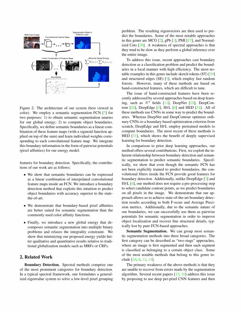
Figure 3: In order to understand, which layers contributemost heavily to the boundary detection, we visualize theweight magnitudes corresponding to each layer in the FCN.The layers are sorted from the earliest to the deepest. Notethat the weight magnitudes corresponding to the deepestlayers of the network are slightly larger than weights fromthe other layers. Since the deepest layers in the FCN arethose most related to prediction of semantic segmentation,this suggests that semantic segmentation cues are beneficialfor the boundary detection task.

we introduce a global energy function, which minimizes theenergy corresponding to the unary and pairwise terms andimproves the initial FCN segmentation. The detailed illus-tration of our architecture is presented in Figure 2. We nowexplain each of these steps in more detail.

3.1. FCN Unary Potentials

To predict semantic unary potentials we employ theDeepLab model [7], which is a fully convolutional adapta-tion of the VGG network [29]. The FCN consists of 16 con-volutional layers and 3 fully convolutional layers. There aremore recent FCN-based methods that have demonstratedeven better semantic segmentation results [8, 32, 16, 21].Although these more advanced architectures could be in-tegrated into our framework to improve our unary poten-tials, in this work we focus on two aspects orthogonal tothis prior work: 1) demonstrating that our boundary-basedaffinity function is better suited for semantic segmentationthan the common color-based affinities and 2) showing thatour proposed global energy achieves better qualitative andquantitative semantic segmentation results in comparison toprior globalization models.

3.2. Boundary Pairwise Potentials

In this section, we describe our approach for buildingpairwise pixel affinities using semantic boundaries. The ba-sic idea behind our boundary detection approach is to ex-press semantic boundaries as a function of convolutional

feature maps inside the FCN. Due to the close relationshipbetween the tasks of semantic segmentation and boundarydetection, we hypothesize that convolutional feature mapsfrom the semantic segmentation FCN can be employed asfeatures for boundary detection.

3.2.1 Learning to Predict Semantic Boundaries.

We propose to express semantic boundaries as a linear com-bination of interpolated FCN feature maps with a non-linearfunction applied on top of this sum. We note that interpo-lation of feature maps has been successfully used in priorwork (see e.g. [15]) in order to obtain dense pixel-level fea-tures from the low-resolution outputs of deep convolutionallayers. Here we adopt interpolation to produce pixel-levelboundary predictions. There are several advantages to ourproposed formulation. First, because we express boundariesas a linear combination of feature maps, we only need tolearn a small number of parameters, corresponding to theindividual weight values of each feature map in the FCN.This amounts to ≈ 5K learning parameters, which is muchsmaller than the number of parameters in the entire network(≈ 15M ). This implies that we can perform boundary de-tection and then use these boundaries to improve semanticsegmentation with little added training cost.

Additionally, expressing semantic boundaries as a linearcombination of FCN feature maps allows us to efficientlypredict boundary probabilities for all pixels in the image(we resize the FCN feature maps to the original image di-mensions). This eliminates the need to select candidateboundary points in a pre-processing stage, which was in-stead required in prior boundary detection work [3, 4].

We train our boundary detector on the BSDS 500dataset [23], which includes ground truth annotations by5 human labelers for each image. The dataset contains200 training, 100 validation, and 200 testing images. Tolearn the weights corresponding to each convolutional fea-ture map we first sample 80K points from the dataset. Wedefine the target labels for each point as the fraction of hu-man annotators agreeing on that point being a boundary. Tofix the issue of label imbalance (there are many more non-boundaries than boundaries), we divide the label space intofour quartiles, and select an equal number of samples foreach quartile to balance the training dataset. Given thesesampled points, we then define our features as the values inthe interpolated convolutional feature maps correspondingto these points. To predict semantic boundaries we weigheach convolutional feature map by its weight, sum them upand apply a sigmoid function on top of it. We obtain theweights corresponding to each convolutional feature map byminimizing the cross-entropy loss using a stochastic batchgradient descent for 50 epochs. To obtain crisper bound-aries at test-time we post-process the boundary probabilities

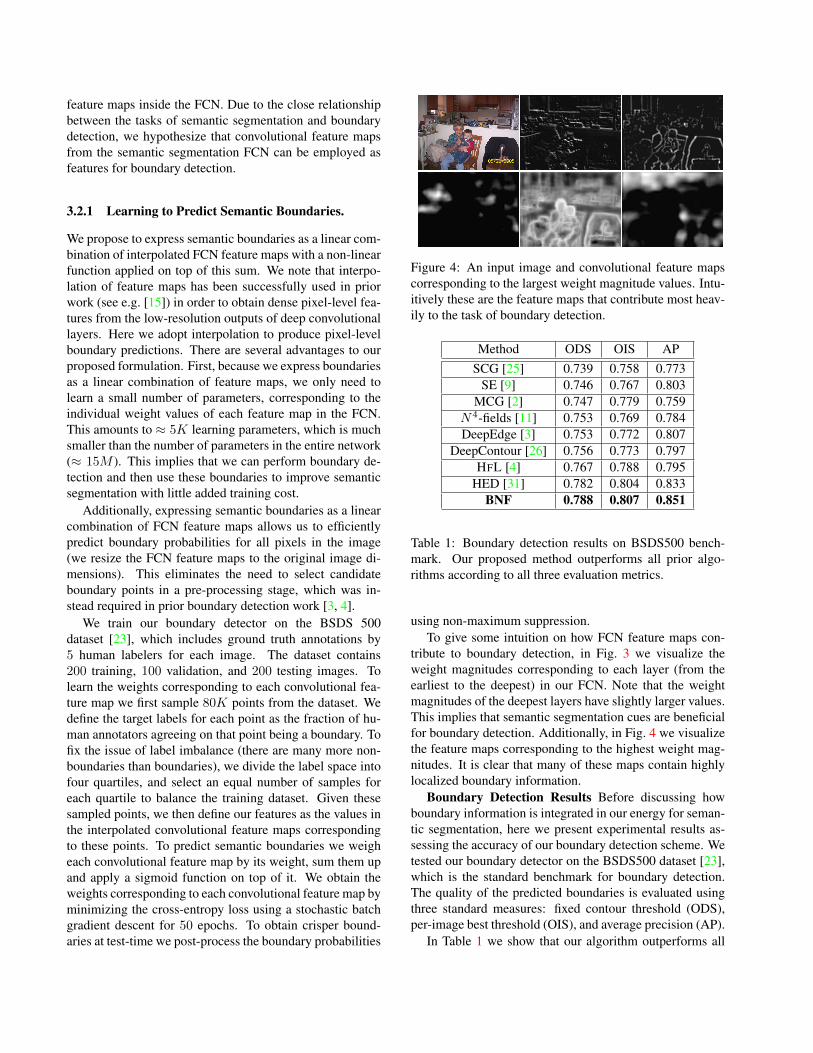
Figure 4: An input image and convolutional feature mapscorresponding to the largest weight magnitude values. Intu-itively these are the feature maps that contribute most heav-ily to the task of boundary detection.

Method ODS OIS APSCG [25] 0.739 0.758 0.773

SE [9] 0.746 0.767 0.803MCG [2] 0.747 0.779 0.759

N4-fields [11] 0.753 0.769 0.784DeepEdge [3] 0.753 0.772 0.807

DeepContour [26] 0.756 0.773 0.797HFL [4] 0.767 0.788 0.795

HED [31] 0.782 0.804 0.833BNF 0.788 0.807 0.851

Table 1: Boundary detection results on BSDS500 bench-mark. Our proposed method outperforms all prior algo-rithms according to all three evaluation metrics.

using non-maximum suppression.To give some intuition on how FCN feature maps con-

tribute to boundary detection, in Fig. 3 we visualize theweight magnitudes corresponding to each layer (from theearliest to the deepest) in our FCN. Note that the weightmagnitudes of the deepest layers have slightly larger values.This implies that semantic segmentation cues are beneficialfor boundary detection. Additionally, in Fig. 4 we visualizethe feature maps corresponding to the highest weight mag-nitudes. It is clear that many of these maps contain highlylocalized boundary information.

Boundary Detection Results Before discussing howboundary information is integrated in our energy for seman-tic segmentation, here we present experimental results as-sessing the accuracy of our boundary detection scheme. Wetested our boundary detector on the BSDS500 dataset [23],which is the standard benchmark for boundary detection.The quality of the predicted boundaries is evaluated usingthree standard measures: fixed contour threshold (ODS),per-image best threshold (OIS), and average precision (AP).

In Table 1 we show that our algorithm outperforms all

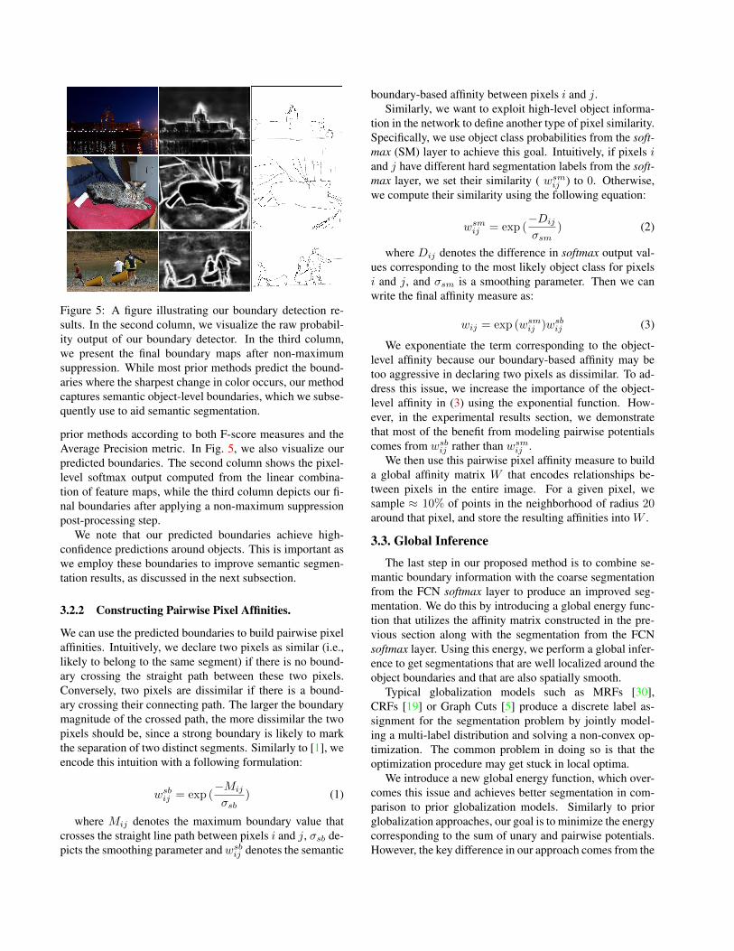
Figure 5: A figure illustrating our boundary detection re-sults. In the second column, we visualize the raw probabil-ity output of our boundary detector. In the third column,we present the final boundary maps after non-maximumsuppression. While most prior methods predict the bound-aries where the sharpest change in color occurs, our methodcaptures semantic object-level boundaries, which we subse-quently use to aid semantic segmentation.

prior methods according to both F-score measures and theAverage Precision metric. In Fig. 5, we also visualize ourpredicted boundaries. The second column shows the pixel-level softmax output computed from the linear combina-tion of feature maps, while the third column depicts our fi-nal boundaries after applying a non-maximum suppressionpost-processing step.

We note that our predicted boundaries achieve high-confidence predictions around objects. This is important aswe employ these boundaries to improve semantic segmen-tation results, as discussed in the next subsection.

3.2.2 Constructing Pairwise Pixel Affinities.

We can use the predicted boundaries to build pairwise pixelaffinities. Intuitively, we declare two pixels as similar (i.e.,likely to belong to the same segment) if there is no bound-ary crossing the straight path between these two pixels.Conversely, two pixels are dissimilar if there is a bound-ary crossing their connecting path. The larger the boundarymagnitude of the crossed path, the more dissimilar the twopixels should be, since a strong boundary is likely to markthe separation of two distinct segments. Similarly to [1], weencode this intuition with a following formulation:

wsbij = exp (−Mij

σsb) (1)

where Mij denotes the maximum boundary value thatcrosses the straight line path between pixels i and j, σsb de-picts the smoothing parameter andwsbij denotes the semantic

boundary-based affinity between pixels i and j.Similarly, we want to exploit high-level object informa-

tion in the network to define another type of pixel similarity.Specifically, we use object class probabilities from the soft-max (SM) layer to achieve this goal. Intuitively, if pixels iand j have different hard segmentation labels from the soft-max layer, we set their similarity ( wsmij ) to 0. Otherwise,we compute their similarity using the following equation:

wsmij = exp (−Dij

σsm) (2)

where Dij denotes the difference in softmax output val-ues corresponding to the most likely object class for pixelsi and j, and σsm is a smoothing parameter. Then we canwrite the final affinity measure as:

wij = exp (wsmij )wsbij (3)

We exponentiate the term corresponding to the object-level affinity because our boundary-based affinity may betoo aggressive in declaring two pixels as dissimilar. To ad-dress this issue, we increase the importance of the object-level affinity in (3) using the exponential function. How-ever, in the experimental results section, we demonstratethat most of the benefit from modeling pairwise potentialscomes from wsbij rather than wsmij .

We then use this pairwise pixel affinity measure to builda global affinity matrix W that encodes relationships be-tween pixels in the entire image. For a given pixel, wesample ≈ 10% of points in the neighborhood of radius 20around that pixel, and store the resulting affinities into W .

3.3. Global Inference

The last step in our proposed method is to combine se-mantic boundary information with the coarse segmentationfrom the FCN softmax layer to produce an improved seg-mentation. We do this by introducing a global energy func-tion that utilizes the affinity matrix constructed in the pre-vious section along with the segmentation from the FCNsoftmax layer. Using this energy, we perform a global infer-ence to get segmentations that are well localized around theobject boundaries and that are also spatially smooth.

Typical globalization models such as MRFs [30],CRFs [19] or Graph Cuts [5] produce a discrete label as-signment for the segmentation problem by jointly model-ing a multi-label distribution and solving a non-convex op-timization. The common problem in doing so is that theoptimization procedure may get stuck in local optima.

We introduce a new global energy function, which over-comes this issue and achieves better segmentation in com-parison to prior globalization models. Similarly to priorglobalization approaches, our goal is to minimize the energycorresponding to the sum of unary and pairwise potentials.However, the key difference in our approach comes from the

relaxation of some of the constraints. Specifically, insteadof modeling our problem as a joint multi-label distribution,we propose to decompose it into multiple binary problems,which can be solved concurrently. This decomposition canbe viewed as assigning pixels to foreground and backgroundlabels for each of the different object classes. Additionally,we relax the integrality constraint. Both of these relaxationsmake our problem more manageable and allow us to formu-late a global energy function that is differentiable, and hasa closed form solution.

In [33], the authors introduce the idea of learningwith global and local consistency in the context of semi-supervised problems. Inspired by this work, we incorporatesome of these ideas in the context of semantic segmenta-tion. Before defining our proposed global energy function,we introduce some relevant notation.

For the purpose of illustration, suppose that we only havetwo classes: foreground and background. Then we can de-note an optimal continuous solution to such a segmentationproblem with variable z∗. To denote similarity between pix-els i and j we use wij . Then, di indicates the degree of apixel i. In graph theory, the degree of a node denotes thenumber of edges incident to that node. Thus, we set the de-gree of a pixel to di =

∑nj=1 wij for all j except i 6= j.

Finally, with fi we denote an initial segmentation proba-bility, which in our case is obtained from the FCN softmaxlayer.

Using this notation, we can then formulate our globalinference objective as:

z∗ = argminz

µ

2

∑

i

di(zi−fidi)2+

1

2

∑

ij

wij(zi−zj)2 (4)

This energy consists of two different terms. Similar tothe general globalization framework, our first term encodesthe unary energy while the second term includes the pair-wise energy. We now explain the intuition behind each ofthese terms. The unary term attempts to find a segmentationassignment (zi) that deviates little from the initial candidatesegmentation computed from the softmax layer (denoted byfi). The zi in the unary term is weighted by the degree diof the pixel in order to produce larger unary costs for pixelsthat have many similar pixels within the neighborhood. In-stead, the pairwise term ensures that pixels that are similarshould be assigned similar z values. To balance the ener-gies of the two terms we introduce a parameter µ and set itto 0.025 throughout all our experiments.

We can also express the same global energy function inmatrix notation:

z∗ = argminz

µ

2D(z−D−1f)T(z−D−1f)+

1

2zT(D−W)z

(5)

where z∗ is a n × 1 vector containing an optimal con-tinuous assignment for all n pixels, D is a diagonal degreematrix, and W is the n× n pixel affinity matrix. Finally, fdenotes a n× 1 vector containing the probabilities from thesoftmax layer corresponding to a particular object class.

An advantage of our energy is that it is differentiable. Ifwe denote the above energy as E(z) then the derivative ofthis energy can be written as follows:

∂E(z)

∂z= µD(z−D−1f) + (D−W)z = 0 (6)

With simple algebraic manipulations we can then obtaina closed form solution to this optimization:

z∗ = (D− αW)−1βf (7)

where α = 11+µ and β = µ

1+µ . In the general case wherewe have k object classes we can write the solution as:

Z∗ = (D− αW)−1βF (8)

where Z now depicts a n × k matrix containing assign-ments for all k object classes, while F denotes n×k matrixwith object class probabilities from softmax layer. Due tothe large size of D−αW it is impractical to invert it. How-ever, if we consider an image as a graph where each pixeldenotes a vertex in the graph, we can observe that the termD−W in our optimization is equivalent to a Laplacian ma-trix of such graph. Since we know that a Laplacian matrix ispositive semi-definite, we can use the preconditioned con-jugate gradient method [27] to solve the system in Eq. (9).Alternatively, because our defined global energy in Eq. (5)is differentiable, we can efficiently solve this optimizationproblem using stochastic gradient descent. We choose theformer option and solve the following system:

(D− αW)z∗ = βf (9)

To obtain the final discrete segmentation, for each pixelwe assign the object class that corresponds to the largestcolumn value in the row of Z (note that each row in Z rep-resents a single pixel in the image, and each column in Zrepresents one of the object classes). In the experimentalsection, we show that this solution produces better quantita-tive and qualitative results in comparison to commonly usedglobalization techniques.

4. Experimental ResultsIn this section we present quantitative and qualitative re-

sults for semantic segmentation on the SBD [13] dataset,which contains objects and their per-pixel annotations for20 Pascal VOC classes. We evaluate semantic segmenta-tion results using two evaluation metrics. The first metric

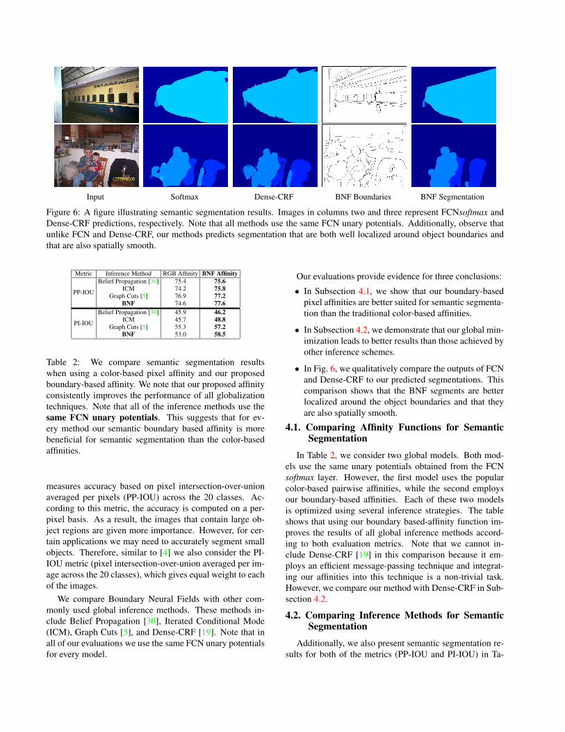
Input Softmax Dense-CRF BNF Boundaries BNF Segmentation

Figure 6: A figure illustrating semantic segmentation results. Images in columns two and three represent FCNsoftmax andDense-CRF predictions, respectively. Note that all methods use the same FCN unary potentials. Additionally, observe thatunlike FCN and Dense-CRF, our methods predicts segmentation that are both well localized around object boundaries andthat are also spatially smooth.

Metric Inference Method RGB Affinity BNF Affinity

PP-IOU

Belief Propagation [30] 75.4 75.6ICM 74.2 75.8

Graph Cuts [5] 76.9 77.2BNF 74.6 77.6

PI-IOU

Belief Propagation [30] 45.9 46.2ICM 45.7 48.8

Graph Cuts [5] 55.3 57.2BNF 53.0 58.5

Table 2: We compare semantic segmentation resultswhen using a color-based pixel affinity and our proposedboundary-based affinity. We note that our proposed affinityconsistently improves the performance of all globalizationtechniques. Note that all of the inference methods use thesame FCN unary potentials. This suggests that for ev-ery method our semantic boundary based affinity is morebeneficial for semantic segmentation than the color-basedaffinities.

measures accuracy based on pixel intersection-over-unionaveraged per pixels (PP-IOU) across the 20 classes. Ac-cording to this metric, the accuracy is computed on a per-pixel basis. As a result, the images that contain large ob-ject regions are given more importance. However, for cer-tain applications we may need to accurately segment smallobjects. Therefore, similar to [4] we also consider the PI-IOU metric (pixel intersection-over-union averaged per im-age across the 20 classes), which gives equal weight to eachof the images.

We compare Boundary Neural Fields with other com-monly used global inference methods. These methods in-clude Belief Propagation [30], Iterated Conditional Mode(ICM), Graph Cuts [5], and Dense-CRF [19]. Note that inall of our evaluations we use the same FCN unary potentialsfor every model.

Our evaluations provide evidence for three conclusions:

• In Subsection 4.1, we show that our boundary-basedpixel affinities are better suited for semantic segmenta-tion than the traditional color-based affinities.

• In Subsection 4.2, we demonstrate that our global min-imization leads to better results than those achieved byother inference schemes.

• In Fig. 6, we qualitatively compare the outputs of FCNand Dense-CRF to our predicted segmentations. Thiscomparison shows that the BNF segments are betterlocalized around the object boundaries and that theyare also spatially smooth.

4.1. Comparing Affinity Functions for SemanticSegmentation

In Table 2, we consider two global models. Both mod-els use the same unary potentials obtained from the FCNsoftmax layer. However, the first model uses the popularcolor-based pairwise affinities, while the second employsour boundary-based affinities. Each of these two modelsis optimized using several inference strategies. The tableshows that using our boundary based-affinity function im-proves the results of all global inference methods accord-ing to both evaluation metrics. Note that we cannot in-clude Dense-CRF [19] in this comparison because it em-ploys an efficient message-passing technique and integrat-ing our affinities into this technique is a non-trivial task.However, we compare our method with Dense-CRF in Sub-section 4.2.

4.2. Comparing Inference Methods for SemanticSegmentation

Additionally, we also present semantic segmentation re-sults for both of the metrics (PP-IOU and PI-IOU) in Ta-

Metric Method aero bike bird boat bottle bus car cat chair cow table dog horse mbike person plant sheep sofa train tv mean

PP-IOU

FCN-Softmax 80.7 71.6 80.7 71.3 72.9 88.1 81.8 86.6 47.4 82.9 57.9 83.9 79.6 80.4 81.0 64.7 78.2 54.5 80.9 69.9 74.8Belief Propagation [30] 81.4 72.2 82.4 72.2 74.3 88.8 82.4 87.2 48.4 83.8 58.4 84.6 80.5 80.9 81.5 65.1 79.5 55.5 81.5 71.2 75.6

ICM 81.7 72.2 82.8 72.1 75.3 89.6 83.4 87.7 46.3 83.3 58.4 84.6 80.6 81.4 81.5 65.8 79.5 56.0 80.7 74.1 75.8Graph Cuts [5] 82.6 72.3 84.7 73.1 76.7 89.9 83.6 89.3 49.7 85.0 61.1 86.2 82.9 81.3 82.3 67.1 80.5 58.8 82.2 75.1 77.2

Dense-CRF [19] 83.4 71.5 84.9 72.6 76.2 89.5 83.3 89.1 50.4 86.7 61.0 86.8 83.5 81.8 82.3 66.9 82.2 58.2 81.9 75.1 77.3BNF-SB 81.9 72.5 84.9 73.3 76.0 90.3 83.1 89.2 51.2 86.7 61.5 86.6 83.2 81.3 81.9 66.2 81.7 58.6 81.6 75.8 77.4

BNF-SB-SM 82.2 73.1 85.1 73.8 76.7 90.6 83.4 89.5 51.3 86.7 61.4 86.8 83.3 81.7 82.3 67.7 81.9 58.4 82.4 75.4 77.6

PI-IOU

FCN-Softmax 56.9 35.1 47.8 41.1 27.4 51.1 43.4 52.7 22.2 43.1 29.2 54.2 40.5 45.6 59.1 24.2 43.6 24.8 55.9 37.2 41.8Belief Propagation [30] 68.0 38.6 52.9 45.8 31.9 55.9 47.2 58.2 24.6 49.9 31.7 60.2 44.9 50.1 62.4 25.2 49.9 27.6 62.3 42.2 46.2

ICM 65.3 40.9 56.4 45.3 33.7 58.9 49.5 61.9 25.8 53.5 33.2 62.1 48.0 53.2 63.4 24.1 54.8 34.0 63.7 47.7 48.8Graph Cuts [5] 71.6 46.8 65.6 49.6 38.0 72.6 52.7 76.7 32.5 69.6 38.9 74.4 61.4 61.0 66.2 30.3 68.7 41.4 72.2 52.8 57.2

Dense-CRF [19] 68.0 39.5 58.0 45.0 33.4 62.8 47.7 66.0 29.4 60.9 36.0 68.5 54.6 51.4 63.7 28.3 57.6 37.1 65.9 48.2 51.1BNF-SB 71.6 48.1 67.2 52.3 37.8 79.5 52.9 80.8 33.3 71.5 39.5 75.1 65.7 63.4 65.1 31.1 67.5 39.6 73.2 54.7 58.5

BNF-SB-SM 72.0 48.9 66.5 52.9 39.1 79.0 53.4 78.6 32.9 72.2 39.4 74.6 65.9 64.2 65.8 31.7 66.9 39.0 73.1 53.9 58.5

Table 3: Semantic segmentation results on the SBD dataset. We measure the results according to PP-IOU (per pixel) and PI-IOU (per image) evaluation metrics. We use BNF-SB to denote the variant of our method that uses only semantic boundarybased affinities. Additionally, we use BNF-SB-SM to indicate our method that uses boundary and softmax based affinities(See Eq. (3)). Based on these results, we observe that our proposed globalization method outperforms other globalizationtechniques according to both metrics by at least 0.4% and 1.3% respectively. Note that in this experiment, all of the infer-ence methods use the same FCN unary potentials. Additionally, for each method except Dense-CRF (it is challenging toincorporate boundary based affinities into the Dense-CRF framework) we use our boundary based affinities, since those leadto better results.

ble 3. In this comparison, all the techniques use the sameFCN unary potentials. Additionally, all inference methodsexcept Dense-CRF use our affinity measure (since the pre-vious analysis suggested that our affinities yield better per-formance). We use BNF-SB to denote the variant of ourmethod that uses only semantic boundary based affinities.Additionally, we use BNF-SB-SM to indicate the versionof our method that uses both boundary and softmax-basedaffinities (see Eq. (3)).

Based on these results, we observe that our proposedtechnique outperforms all the other globalization methodsaccording to both metrics, by 0.4% and 1.3% respectively.Additionally, these results indicate that most benefit comesfrom the semantic boundary affinity term rather than thesoftmax affinity term.

In Fig. 6, we also present qualitative semantic segmenta-tion results. Note that, compared to the segmentation out-put from the softmax layer, our segmentation is much bet-ter localized around the object boundaries. Additionally,in comparison to Dense-CRF predictions, our method pro-duces segmentations that are much spatially smoother.

4.3. Semantic Boundary Classification

We can also label our boundaries with a specific objectclass, using the same classification strategy as in the HFLsystem [4]. Since the SBD dataset provides annotations forsemantic boundary classification, we can test our resultsagainst the state-of-the-art HFL [4] method for this task.Due to the space limitation, we do not include full results foreach category. However, we observe that our produced re-sults achieve mean Max F-Score of 54.5% (averaged acrossall 20 classes) whereas HFL method obtains 51.7%.

5. Conclusions

In this work we introduced a Boundary Neural Field(BNF), an architecture that employs a semantic segmenta-tion FCN to predict semantic boundaries and then uses thepredicted boundaries and the FCN output to produce an im-proved semantic segmentation maps a global optimization.We showed that our predicted boundaries are better suitedfor semantic segmentation than the commonly used low-level color based affinities. Additionally, we introduced aglobal energy function that decomposes semantic segmen-tation into multiple binary problems and relaxes an inte-grality constraint. We demonstrated that the minimizationof this global energy allows us to predict segmentationsthat are better localized around the object boundaries andthat are spatially smoother compared to the segmentationsachieved by prior methods.

The main goal of this work was to show the effective-ness of boundary-based affinities for semantic segmenta-tion. However, due to differentiability of our global energy,it may be possible to add more parameters inside the BNFsand learn them in a front-to-end fashion. We believe thatoptimizing the entire architecture jointly could capture theinherent relationship between semantic segmentation andboundary detection even better and further improve the per-formance of BNFs. We will investigate this possibility inour future work.

References[1] Pablo Arbelaez, Michael Maire, Charless Fowlkes, and Jitendra Ma-

lik. Contour detection and hierarchical image segmentation. IEEETrans. Pattern Anal. Mach. Intell., 33(5):898–916, May 2011. 2, 5

[2] Pablo Arbelaez, J. Pont-Tuset, Jon Barron, F. Marqués, and JitendraMalik. Multiscale combinatorial grouping. In Computer Vision andPattern Recognition (CVPR), 2014. 2, 4

[3] Gedas Bertasius, Jianbo Shi, and Lorenzo Torresani. Deepedge: Amulti-scale bifurcated deep network for top-down contour detection.In The IEEE Conference on Computer Vision and Pattern Recogni-tion (CVPR), June 2015. 2, 4

[4] Gedas Bertasius, Jianbo Shi, and Lorenzo Torresani. High-for-lowand low-for-high: Efficient boundary detection from deep object fea-tures and its applications to high-level vision. In The IEEE Interna-tional Conference on Computer Vision (ICCV), December 2015. 2,4, 7, 8

[5] Yuri Boykov, Olga Veksler, and Ramin Zabih. Fast approximate en-ergy minimization via graph cuts. IEEE Trans. Pattern Anal. Mach.Intell., 23(11):1222–1239, November 2001. 5, 7, 8

[6] João Carreira, Rui Caseiro, Jorge Batista, and Cristian Sminchisescu.Semantic segmentation with second-order pooling. In Proceedingsof the 12th European Conference on Computer Vision - Volume PartVII, ECCV’12, pages 430–443, Berlin, Heidelberg, 2012. Springer-Verlag. 2

[7] Liang-Chieh Chen, George Papandreou, Iasonas Kokkinos, KevinMurphy, and Alan L. Yuille. Semantic image segmentation with deepconvolutional nets and fully connected crfs. CoRR, abs/1412.7062,2014. 1, 2, 3

[8] Jifeng Dai, Kaiming He, and Jian Sun. Boxsup: Exploiting bound-ing boxes to supervise convolutional networks for semantic segmen-tation. CoRR, abs/1503.01640, 2015. 3

[9] Piotr Dollár and C. Lawrence Zitnick. Fast edge detection usingstructured forests. PAMI, 2015. 2, 4

[10] Clement Farabet, Camille Couprie, Laurent Najman, and Yann Le-Cun. Learning hierarchical features for scene labeling. IEEE Trans-actions on Pattern Analysis and Machine Intelligence, August 2013.2

[11] Yaroslav Ganin and Victor S. Lempitsky. N4-fields: Neural networknearest neighbor fields for image transforms. ACCV, 2014. 2, 4

[12] Saurabh Gupta, Ross Girshick, Pablo Arbeláez, and Jitendra Malik.Learning rich features from RGB-D images for object detection andsegmentation. In Proceedings of the European Conference on Com-puter Vision (ECCV), 2014. 2

[13] Bharath Hariharan, Pablo Arbelaez, Lubomir Bourdev, SubhransuMaji, and Jitendra Malik. Semantic contours from inverse detectors.In International Conference on Computer Vision (ICCV), 2011. 6

[14] Bharath Hariharan, Pablo Arbeláez, Ross Girshick, and Jitendra Ma-lik. Simultaneous detection and segmentation. In European Confer-ence on Computer Vision (ECCV), 2014. 2

[15] Bharath Hariharan, Pablo Andrés Arbeláez, Ross B. Girshick, andJitendra Malik. Hypercolumns for object segmentation and fine-grained localization. CoRR, abs/1411.5752, 2014. 2, 4

[16] Seunghoon Hong, Hyeonwoo Noh, and Bohyung Han. Decou-pled deep neural network for semi-supervised semantic segmenta-tion. arXiv preprint arXiv:1506.04924, 2015. 3

[17] Phillip Isola, Daniel Zoran, Dilip Krishnan, and Edward H. Adelson.Crisp boundary detection using pointwise mutual information. InECCV, 2014. 2

[18] Jyri J Kivinen, Christopher KI Williams, Nicolas Heess, and Deep-Mind Technologies. Visual boundary prediction: A deep neural pre-diction network and quality dissection. AISTATS, 1(2):9, 2014. 2

[19] Philipp Krähenbühl and Vladlen Koltun. Efficient inference in fullyconnected crfs with gaussian edge potentials. In J. Shawe-Taylor,R.S. Zemel, P.L. Bartlett, F. Pereira, and K.Q. Weinberger, editors,Advances in Neural Information Processing Systems 24, pages 109–117. Curran Associates, Inc., 2011. 1, 5, 7, 8

[20] Joseph Lim, C. Lawrence Zitnick, and Piotr Dollár. Sketch tokens:A learned mid-level representation for contour and object detection.In CVPR, 2013. 2

[21] Guosheng Lin, Chunhua Shen, Ian D. Reid, and Anton van den Hen-gel. Efficient piecewise training of deep structured models for se-mantic segmentation. CoRR, abs/1504.01013, 2015. 3

[22] Jonathan Long, Evan Shelhamer, and Trevor Darrell. Fully convo-lutional networks for semantic segmentation. CVPR (to appear),November 2015. 1, 3

[23] D. Martin, C. Fowlkes, D. Tal, and J. Malik. A database of humansegmented natural images and its application to evaluating segmen-tation algorithms and measuring ecological statistics. In Proc. 8thInt’l Conf. Computer Vision, volume 2, pages 416–423, July 2001. 4

[24] Mohammadreza Mostajabi, Payman Yadollahpour, and GregoryShakhnarovich. Feedforward semantic segmentation with zoom-outfeatures. CoRR, abs/1412.0774, 2014. 2

[25] X. Ren and L. Bo. Discriminatively Trained Sparse Code Gradientsfor Contour Detection. In Advances in Neural Information Process-ing Systems, December 2012. 4

[26] Wei Shen, Xinggang Wang, Yan Wang, Xiang Bai, and ZhijiangZhang. Deepcontour: A deep convolutional feature learned bypositive-sharing loss for contour detection. June 2015. 2, 4

[27] Jonathan R Shewchuk. An introduction to the conjugate gradientmethod without the agonizing pain. Technical report, Pittsburgh, PA,USA, 1994. 6

[28] Jianbo Shi and Jitendra Malik. Normalized cuts and image segmen-tation. IEEE Transactions on Pattern Analysis and Machine Intelli-gence, 22:888–905, 1997. 2

[29] K. Simonyan and A. Zisserman. Very deep convolutional networksfor large-scale image recognition. CoRR, abs/1409.1556, 2014. 3

[30] Marshall F. Tappen and William T. Freeman. Comparison of graphcuts with belief propagation for stereo, using identical mrf parame-ters. In Proceedings of the Ninth IEEE International Conference onComputer Vision - Volume 2, ICCV ’03, pages 900–, Washington,DC, USA, 2003. IEEE Computer Society. 5, 7, 8

[31] Saining Xie and Zhuowen Tu. Holistically-nested edge detection.CoRR, abs/1504.06375, 2015. 2, 4

[32] Shuai Zheng, Sadeep Jayasumana, Bernardino Romera-Paredes, Vib-hav Vineet, Zhizhong Su, Dalong Du, Chang Huang, and Philip Torr.Conditional random fields as recurrent neural networks. In Interna-tional Conference on Computer Vision (ICCV), 2015. 3

[33] Dengyong Zhou, Olivier Bousquet, Thomas N. Lal, Jason Weston,and Bernhard Schölkopf. Learning with local and global consistency.In S. Thrun, L.K. Saul, and B. Schölkopf, editors, Advances in Neu-ral Information Processing Systems 16, pages 321–328. MIT Press,2004. 6