
Models for the assessment of seismic vulnerability of old ...
Upload
truongminhCategory
view
228download
1
September 2007
Seismic Vulnerability Assessment of Structures using Operational Modal Analysis
Taking the Guesswork Out of Future Earthquakes
FILIPE DUARTE MATIAS ÂNGELO
Dissertation for the Master of Science degree in
CIVIL ENGINEERING
Supervisor (AAU, Denmark):
Prof. Rune Brincker
Jury
President: Prof. Pedro Guilherme Sampaio Viola Parreira
Supervisor (IST, TU Lisbon): Prof. Jorge Miguel Silveira Filipe Mascarenhas Proença
Assessor: Prof. Alfredo Peres de Noronha Campos Costa


The present thesis constitutes an
integrated part of the studies for the
Master Degree in Civil Engineering at
Instituto Superior Técnico


Contents
i
Contents
Contents...................................................................................................................................... i
Abstract / Resumo..................................................................................................................... v
Nomenclature ........................................................................................................................... ix
List of Figures.........................................................................................................................xiii
List of Tables .........................................................................................................................xvii
1 Introduction ..........................................................................................................................1 1.1 Foreword......................................................................................................................1 1.2 Motivation for this study ...............................................................................................2 1.3 Objective ......................................................................................................................2 1.4 Stating the Problem .....................................................................................................4 1.5 Organization of the Thesis...........................................................................................6
2 Seismic Vulnerability Assessment.....................................................................................7 2.1 Introduction ..................................................................................................................7 2.2 Earthquakes.................................................................................................................8
2.2.1 Geographical Distribution of Earthquakes ......................................................8 2.2.2 Types of Earthquakes .....................................................................................9
2.2.2.1 Natural Earthquakes .........................................................................9 2.2.2.2 Induced Earthquakes ......................................................................11
2.3 Analysis procedures...................................................................................................11 2.3.1 Linear Elastic Analyses.................................................................................12 2.3.2 Nonlinear Analyses .......................................................................................12
2.3.2.1 Nonlinear Static Analysis...............................................................13 2.3.2.1.1 Push-Over Analysis ......................................................15 2.3.2.1.2 Fragility Curves.............................................................16

Seismic Vulnerability Assessment of Structures using Operational Modal Analysis
ii
3 Operational Modal Analysis ..............................................................................................17 3.1 Introduction ................................................................................................................17 3.2 Applications of OMA for Structural Identification .......................................................18 3.3 Identification Techniques ...........................................................................................20
3.3.1 Non-Parametric Techniques .........................................................................20 3.3.2 Parametric Techniques .................................................................................21
3.4 Frequency Domain Decomposition (FDD) .................................................................22 3.5 Case Study – Laboratory Model ................................................................................27
3.5.1 Description of the Laboratory Model .............................................................27 3.5.2 Data Processing and Modal Identification Procedures .................................28
4 Fragility Curves ..................................................................................................................33 4.1 Scope .........................................................................................................................33 4.2 Procedure...................................................................................................................34 4.3 Case study .................................................................................................................35
4.3.1 Model Description..........................................................................................35 4.3.2 Model Building Type Classification ...............................................................36 4.3.3 Building Damage States (C1L)......................................................................36 4.3.4 Seismic Design Level ....................................................................................37 4.3.5 Push-Over Curve to Capacity Curve.............................................................38 4.3.6 Fragility Curves .............................................................................................41 4.3.7 Elastic Response Spectrum ..........................................................................42 4.3.8 Solicitation Spectrum.....................................................................................43 4.3.9 Probability of Damage...................................................................................45 4.3.10 Procedure according to HAZUS:...................................................................47
4.3.10.1 Capacity Curve..............................................................................47 4.3.10.2 Fragility Curves .............................................................................49 4.3.10.3 Response Spectrum......................................................................50 4.3.10.4 Solicitation Spectrum ....................................................................51 4.3.10.5 Structural Response Estimation....................................................53
4.3.11 Procedure according to HAZUS using analytical period estimation: ............56 4.3.11.1 Capacity Curve..............................................................................56 4.3.11.2 Fragility Curves .............................................................................58 4.3.11.3 Response Spectrum......................................................................59 4.3.11.4 Solicitation Spectrum ....................................................................60 4.3.11.5 Structural Response Estimation....................................................61 4.3.11.6 Sub-Conclusion..............................................................................64
4.3.12 Procedure according to HAZUS using an higher period value: ....................65 4.3.12.1 Capacity Curve..............................................................................65 4.3.12.2 Fragility Curves .............................................................................66 4.3.12.3 Response Spectrum......................................................................68

Contents
iii
4.3.12.4 Solicitation Spectrum ....................................................................69 4.3.12.5 Structural Response Estimation ...................................................70 4.3.12.6 Sub-Conclusion.............................................................................73
4.4 Error Prediction and Evaluation Introducing OMA Information..................................73 4.4.1 Fragility Curves out of HAZUS Guidelines....................................................73 4.4.2 Fragility Curves out of Operational Modal Analysis ......................................74
4.4.2.1 Error Estimation in Modal Identification ..........................................75
5 Summary and Conclusions...............................................................................................77 5.1 Summary....................................................................................................................77 5.2 Conclusions ...............................................................................................................78 5.3 Recommendations for Future Researches................................................................80
References ...............................................................................................................................81
Appendix A: Seismic Waves ..................................................................................................83
Appendix B: Earthquake Magnitude .....................................................................................89
Appendix C: Earthquake Intensity.........................................................................................91
Appendix D: Introduction to Linear Waves ..........................................................................97
Appendix E: Singular Value Decomposition, SVD.............................................................105
Appendix F: Eigenfrequencies ............................................................................................109

Seismic Vulnerability Assessment of Structures using Operational Modal Analysis
iv

Abstract
v
Abstract
The techniques and analytical algorithms used to perform dynamic analysis in structures have
suffered an extreme improvement during the last decades, particularly in the field of dynamic
identification of structural systems.
This document presents a practical assessment of the seismic performance of structural
systems proposing a new damage evaluation method using Operational Modal Analysis and the
guidelines provided by FEMA – “HAZUS-MH MR1 Technical Manual” [FEMA, 2003].
Performance is measured in terms of the likelihood that a building, given a certain level of
ground motion, can be in one of the five structural limit states proposed. The link between the
patterns of structural damage and the assignment of the appropriate limit state is made using
the loss of capacity of the structure after the main shock, which allow the quantitative
measurement of the performance degradation.
On one hand, this work will introduce the basic concepts about earthquake engineering and the
human need to control such levels of vibration. On the other hand, it will concentrate on the
Operational Modal Analysis domain. With this modern tool, engineers can estimate the level of
vibration acting in a real structure in an expedite way, allowing to know about its dynamic
characteristics.
Furthermore, this thesis will try to act as a bridge between these two domains of study in
engineering, trying to achieve a reasonable co-existence between the linear and nonlinear
analysis methods and verify the improvement of accuracy obtainable if using real data
acquisition in the damage assessment method.
As a mere practical application of O.M.A., ambient vibration tests will be performed in a reduced
model of three storeys. The numerical results are in excellent agreement with the expected data
and show that future successful testing can be performed.
Keywords: Operational Modal Analysis, Damage Assessment, Capacity Curve, Fragility
Curves, Frequency Domain Decomposition (FDD)

Seismic Vulnerability Assessment of Structures using Operational Modal Analysis
vi

Resumo
vii
Resumo
As técnicas e algoritmos analíticos usados em análises dinâmicas de estruturas têm sofrido um
extremo avanço durante as últimas décadas, particularmente no campo da identificação
dinâmica de sistemas estruturais.
Este documento apresenta uma abordagem prática da avaliação do desempenho de estruturas
em cenário sísmico propondo um novo método para avaliação de dano estrutural tirando
partido da Análise Modal Operacional e dos regulamentos propostos pela FEMA: “HAZUS-MH
MR1 Technical Manual” [FEMA, 2003]. O desempenho é avaliado em termos da
susceptibilidade do edifício, dado um certo nível de vibração do solo, poder estar dentro de um
dos cinco estados estruturais limite propostos pelo mesmo regulamento. A ligação entre os
padrões de dano estrutural e a atribuição do estado limite apropriado é feita de acordo com a
perda de capacidade da estrutura depois de um primeiro choque, o que permite a análise
quantitativa da degradação do desempenho estrutural. A perda de capacidade do sistema será
avaliada através do conceito de curva de capacidade.
Por um lado, este trabalho irá abordar os conceitos básicos de engenharia sísmica e a
necessidade humana de controlar certos níveis de vibração. Por outro lado, irá concentrar-se
no domínio da Análise Modal Operacional. Com esta moderna ferramenta de engenharia, será
possível estimar o nível de vibração actuante numa estrutura real de uma forma expedita e
bastante aproximada.
Adicionalmente, a presente dissertação poderá ser vista como uma primeira abordagem
relativa à possível ligação entre estes dois domínios da engenharia, onde se tentará encontrar
uma certa coexistência entre o campo da análise linear e da análise não linear.
Como mera aplicação prática da O.M.A., serão realizados testes de vibração ambiente num
modelo reduzido de três pisos. Os resultados numéricos revelam-se em excelente
concordância com os resultados esperados comprovando-se assim que o futuro da análise
modal em estruturas reais é promissor, pois conseguem-se obter valores muito próximos dos
reais. A possível aplicação desta técnica é discutida.
Palavras-Chave: Análise Modal Operacional, Avaliação de Dano, Curva de Capacidade, Curva
de Fragilidade, Decomposição no Domínio da Frequência (FDD)

Seismic Vulnerability Assessment of Structures using Operational Modal Analysis
viii
Nomenclature
ix
Nomenclature
General Rules
- Vector symbols are represented by italic type characters.
- Matrix symbols are represented by bold type characters and capital letters.
- The inverse of a matrix is denoted by the superscript -1.
- The transpose of a matrix is denoted by the superscript T.
- The complex conjugate is denoted by the superscript *.
- The complex conjugate transpose (Hermitian) of a matrix is denoted by the superscript H.
- The mean value is denoted by the superscript A .
- Vectors are generally considered to be column vectors, and the scalar product is denoted
by xTy.
- Continuous-time stochastic processes are denoted by y(t).
- Differentiation with respect to time is symbolized by superscript dots
( )( ) dy ty tdt
= , 2
2
( )( ) d y ty tdt
=
Scalars
x, y Scalar
t, τ Time
μ Mean value
σ Standard deviation
Sd Spectral displacement
Sa Spectral acceleration
S Soil class parameter
Dy Yielding displacement capacity
Du Ultimate displacement capacity
Ay Yielding acceleration capacity
Au Ultimate acceleration capacity
M Effective modal mass
H Effective modal height

Seismic Vulnerability Assessment of Structures using Operational Modal Analysis
x
Cs Design strength coefficient
α1 Fraction of the system’s effective weight
α2 Fraction of the system’s effective height ,B CT T Constant spectral acceleration zone limits
DT Constant spectral displacement initial value
0β Amplification coefficient of spectral acceleration for a certain damping ratio
k1, k2 Parameters that influence spectra for values of CT e DT , respectively.
Vectors and Matrices
x, y Vector
X, Y Matrix
I Identity matrix
A-1 Inverse of a matrix A
aT , AT Transpose of a vector a or a matrix A, respectively
aH , AH Complex conjugate transpose of a vector a or a matrix A, respectively
a* Complex conjugate of a vector a
det (A) Determinant of matrix A
Φ Mode shape matrix
K Stiffness matrix
M Diagonal mass matrix.
Modal Parameters
fi Undamped natural eigenfrequency of the ith mode
ωi Undamped circular eigenfrequency of the ith mode
ξi Damping ratio of the ith eigenvalue
λi ith eigenvalue of a continuous-time system
φi Mode shape corresponding to the ith eigenvalue
T Number of time series.

Nomenclature
xi
Statistical Parameters
P(ds) Discrete probability of being in a certain damage state ds
E[x] Expected value of x
R(x) Correlation function of x
C Covariance Matrix
S(ω) Spectral Density Matrix of an output process
u, U Singular Vector, Matrix of Singular Vectors
y(t) , y (ω) System Response in time domain or frequency domain, respectively
{ }( )X τℑ Fourier Transform of a function (in time domain).
Abbreviations and Acronyms ds – Structural Damage State
FFD – Frequency Domain Decomposition
OMA – Operational Modal Analysis / Output-Only Modal Analysis
CEN – European Committee for Standardization (Comité Européen de Normalisation)
FEMA – Federal Emergency Management Agency
ARTeMIS – Ambient Response Testing and Modal Identification Software.

Seismic Vulnerability Assessment of Structures using Operational Modal Analysis
xii

List of Figures
xiii
List of Figures
Figure 1 – Procedure Scheme ...................................................................................................... 5
Figure 2 – Earthquake epicentres in the last decade: 358214 events.......................................... 8
Figure 3 – Epicentre and Hypocentre of an Earthquake............................................................... 9
Figure 4 – Divergent tectonic plates or normal fault ................................................................... 10
Figure 5 – Convergent tectonic plates or reverse (thrust) fault - Subduction phenomena ......... 10
Figure 6 – Lateral displacement between two tectonic plates – Strike-Slip Fault....................... 11
Figure 7 – Main steps in non-parametric technique methods..................................................... 20
Figure 8 – Main steps in parametric technique methods ............................................................ 21
Figure 9 – Steps involved in the procedure from acceleration in time domain to power spectral
densities in frequency domain ................................................................................ 24
Figure 10 – Simple sketch of the reduced lab model and its nodes ........................................... 27
Figure 11 – Perspective view of the real laboratory model and accelerometers detail .............. 28
Figure 12 – Brüel & Kjær accelerometers (Miniature DeltaTron TEDS) used in the model
ambient test ............................................................................................................ 28
Figure 13 – Model with all test setups and all channels.............................................................. 29
Figure 14 – (a) Model with setup 1; (b) Model with setup 2........................................................ 29
Figure 15 – Singular values of spectral density matrices............................................................ 30
Figure 16 – 1st, 2nd and 3rd mode shapes of the reduced model................................................. 31
Figure 17 – 4th, 5th and 6th mode shapes of the reduced model ................................................. 32
Figure 18 – 7th, 8th and 9th mode shapes of the reduced model ................................................. 32
Figure 19 – Simple concrete frame structure adopted [SAP2000 v10]....................................... 35
Figure 20 – Capacity Curve ........................................................................................................ 38
Figure 21 – From a MDOF system to a SDOF system............................................................... 40
Figure 22 – Capacity Curve for C1L building type under the Pre-Code seismic design level .... 48
Figure 23 – Fragility Curves for a C1L building type with Pre-Code seismic design .................. 49
Figure 24 – Normalised Response Spectrum in Period-Spectral Acceleration, 5% damping, Soil
Class B.................................................................................................................... 50
Figure 25 – Normalised Response Spectrum in Spectral Displacement-Spectral Acceleration,
5% damping, Soil Class B ...................................................................................... 51
Figure 26 – Bilinear representation of the capacity curve........................................................... 51
Figure 27 – Approximate Hysteretic Diagram representation..................................................... 52
Figure 28 – Response and solicitation spectrums (according to EC8) ....................................... 53

Seismic Vulnerability Assessment of Structures using Operational Modal Analysis
xiv
Figure 29 – C1L model type response estimation for Pre-Code design within short and
moderate seismic action duration ........................................................................... 54
Figure 30 – Fragility curves with Spectral Displacement Response for C1L building type and
Pre-Code design level............................................................................................. 55
Figure 31 – Discrete probabilities of structural damage states for the C1L model with Pre-Code
design level ............................................................................................................. 55
Figure 32 – Capacity Curve for C1L building type under the Pre-Code seismic design level with
calculated elastic fundamental period..................................................................... 58
Figure 33 – Fragility Curves for a C1L building type with Pre-Code seismic design .................. 59
Figure 34 – Bilinear representation of the capacity curve ........................................................... 60
Figure 35 – C1L model type response estimation for Pre-Code design within short and
moderate seismic action duration ........................................................................... 62
Figure 36 – Fragility curves with Spectral Displacement Response for C1L building type and
Pre-Code design level............................................................................................. 63
Figure 37 – Discrete probabilities of structural damage states for the C1L model with Pre-Code
design level ............................................................................................................. 63
Figure 38 – Capacity Curve for C1L building type under the Pre-Code seismic design level .... 66
Figure 39 – Fragility Curves for a C1L building type with Pre-Code seismic design .................. 67
Figure 40 – Normalised Response Spectrum in Spectral Displacement-Spectral Acceleration,
5% damping, Soil Class B....................................................................................... 68
Figure 41 – Bilinear representation of the capacity curve ........................................................... 69
Figure 42 – Response and solicitation spectrums (according to EC8) ....................................... 70
Figure 43 – C1L model type response estimation for Pre-Code design within short and
moderate seismic action duration ........................................................................... 71
Figure 44 – Fragility curves with Spectral Displacement Response for C1L building type and
Pre-Code design level............................................................................................. 72
Figure 45 – Discrete probabilities of structural damage states for the C1L model with Pre-Code
design...................................................................................................................... 72
Figure 46 – Primary wave movement.......................................................................................... 84
Figure 47 – Secondary wave movement..................................................................................... 85
Figure 48 – Rayleigh wave movement ........................................................................................ 86
Figure 49 – Love wave movement .............................................................................................. 87
Figure 50 – Mercalli intensity level I (M1)....................................................................................91
Figure 51 – Mercalli intensity level II (M2)...................................................................................92
Figure 52 – Mercalli intensity level III (M3).................................................................................. 92
Figure 53 – Mercalli intensity level IV (M4) ................................................................................. 92
Figure 54 – Mercalli intensity level V (M5) .................................................................................. 93
Figure 55 – Mercalli intensity level VI (M6) ................................................................................. 93
Figure 56 – Mercalli intensity level VII (M7) ................................................................................ 93
Figure 57 – Mercalli intensity level VIII (M8) ............................................................................... 94
Figure 58 – Mercalli intensity level IX (M9) ................................................................................. 94

List of Figures
xv
Figure 59 – Mercalli intensity level X (M10)...................................................................................... 94
Figure 60 – Mercalli intensity level XI (M11)..................................................................................... 95
Figure 61 – Mercalli intensity level XII (M12).................................................................................... 95
Figure 62 – Superposition of periodic waves.................................................................................. 100
Figure 63 – Variance Diagram........................................................................................................ 101
Figure 64 – Stepped Variance Diagram ......................................................................................... 102
Figure 65 – Continuous Variance Diagram..................................................................................... 102
Figure 66 – Singular Values obtained from the SVD method......................................................... 109
Figure 67 – Auto Spectral Densities obtained with Channel 1 and 1 - S11 ..................................... 110
Figure 68 – Auto Spectral Densities obtained with Channel 2 and 2 – S22 .................................... 111
Figure 69 – Auto Spectral Densities obtained with Channel 3 and 3 – S33 .................................... 111
Figure 70 – Cross Spectral Densities obtained with Channel 1 and 2 – S12 or S21 ........................ 112
Figure 71 – Cross Spectral Densities obtained with Channel 1 and 3 – S13 or S31 ........................ 112
Figure 72 – Cross Spectral Densities obtained with Channel 2 and 3 – S23 or S32 ........................ 113

Seismic Vulnerability Assessment of Structures using Operational Modal Analysis
xvi

List of Tables
xvii
List of Tables
Table 1 – Frequency values for each mode................................................................................ 31 Table 2 – Degradation factor for the effective damping of a C1L building model with a Pre-Code
design........................................................................................................................ 44 Table 3 – Code building capacity parameters: Design Strength (Cs), Period (Te), Push-Over
Mode Response Factors (α1, α2), Overstrength Ratios (ɣ, λ) and Ductility Factor (μ)
for the C1L building type and for Pre-Code Seismic Design..................................... 47 Table 4 – Spectral displacements and spectral accelerations for the yielding and ultimate
capacity points........................................................................................................... 48 Table 5 – Fragility Curve Probabilistic Parameters for a C1L building type................................ 49 Table 6 – Elastic spectral response parameters according to Eurocode 8................................. 50 Table 7 – Effective damping for different soil excitation durations.............................................. 52 Table 8 – Reduction factor for the elastic response spectrum for different soil excitation
durations.................................................................................................................... 52 Table 9 – Spectral peak responses coordinates of the C1L model type for short and moderate
duration of seismic action.......................................................................................... 54 Table 10 – New Building capacity parameters: Design Strength (Cs), Calculated Period (Te),
Push-Over Mode Response Factors (α1, α2), Overstrength Ratios (ɣ, λ) and Ductility
Factor (μ) for the C1L building type and for Pre-Code Seismic Design.................... 57 Table 11 – Spectral displacements and spectral accelerations for the yielding and ultimate
capacity points........................................................................................................... 57 Table 12 – Fragility Curve Probabilistic Parameters................................................................... 59 Table 13 – Elastic spectral response parameters according to Eurocode 8............................... 60 Table 14 – Effective damping for different soil excitation durations............................................ 61 Table 15 – Reduction factors for the elastic response spectrum for different soil excitation
durations.................................................................................................................... 61 Table 16 – Spectral peak responses coordinates of the C1L model type for short and moderate
duration of seismic action.......................................................................................... 62 Table 17 – Code building capacity parameters: Design Strength (Cs), Period (Te), Push-Over
Mode Response Factors (α1, α2), Overstrength Ratios (ɣ, λ) and Ductility Factor (μ)
for the C1L building type and for Pre-Code Seismic Design..................................... 65 Table 18 – Spectral displacements and spectral accelerations for the yielding and ultimate
capacity points........................................................................................................... 65

Seismic Vulnerability Assessment of Structures using Operational Modal Analysis
xviii
Table 19 – Fragility Curve Probabilistic Parameters for a C1L building type.............................. 67 Table 20 – Elastic spectral response parameters according to Eurocode 8............................... 68 Table 21 – Effective damping for different soil excitation durations............................................ 69 Table 22 – Reduction factor for the elastic response spectrum for different soil excitation
durations.................................................................................................................... 70 Table 23 – Spectral peak responses coordinates of the C1L model type for short and moderate
duration of seismic action.......................................................................................... 71 Table 24 – Richter’s Scale (adapted from U.S. Geological Survey documents)......................... 90

Introduction
1
1 Introduction
1.1 FOREWORD
Throughout the history of engineering it is fully well known that vibrations when acting in real
structures result in disturbance, discomfort, damage and destruction. After a large scale
earthquake, evaluation of damage in structures such as buildings and bridges has a great
importance to assure the functionality, security and even emergency escape possibilities.
As this happens, interest in seismic hazard and performance of structures under the action of
an earthquake has steadily increased in recent years. This interest has expanded from the
seismology and earthquake engineering communities to the emergency response
organizations, owners of critical facilities and institutions, media and even to the common
people. Seem like there is a growing need for information concerning the intensity of
earthquakes and their possible effects on structures, especially right after a few minutes of
moderate and large magnitude events.
When it comes to dramatic natural events such as earthquakes, engineers around the world are
aware of the enormous amounts of energy that is released. This energy is transmitted to the
surface by vibrations that can easily be absorbed by common buildings, bridges, dams, and all
other infrastructures founded on the earth’s surface. These structures must be capable to
withstand the maximum expected levels of earthquake excited vibration without collapse in
order to guarantee the security of people and its continuous functionality. Due to this fact,
throughout the last decades, it has been recognized a great effort from engineers to develop
new theories and methods to predict and prevent the inherent consequences that eventually
can cause serious damage in real structures.
The knowledge and understanding of this catastrophic process is definitely important if one
wants to design and build structures combining an economic and seismic resistant solution.

Seismic Vulnerability Assessment of Structures using Operational Modal Analysis
2
1.2 MOTIVATION FOR THIS STUDY
At the top end of the vibrations scale, we can find the earthquake generated vibrations. The
range of vibration that can cause damage in buildings extends from minor cracks to complete
collapse. Therefore, protection against collapse has always been a major concern in the seismic
design. In earthquake engineering, the term “collapse” refers to a structural system’s loss of
capacity to resist gravity loads when subjected to seismic excitation, which can lead to the term
“global collapse” that is usually related with dynamic instability triggered by large story drifts.
Due to the lack of hysteretic models capable of simulating dynamic deteriorating behaviour,
global collapse is usually associated with inter-story drifts or with the exceeding of a limit value
of deformation in a certain element of the structure. These deformations are usually amplified by
second degree effects (P-Δ effects) and deterioration in strength and stiffness of the
components of the structural system are usually verified.
Even though this kind of approach has been reliable enough, it doesn’t allow the engineer to
estimate damage redistribution and doesn’t account for the capacity of the system before
collapse to sustain deformations that are significantly larger than those associated with loss of
resistance in individual elements.
Accordingly, a systematic tool to integrate all the sources provided by earthquake events needs
to be developed.
This present work proposes the damage evaluation method of structures based on modal
identification techniques and the construction of fragility curves which approximately lets us
know the level of damage in structural systems. With these promising tools, it is expected that
the possibility to evaluate the damage in a structure becomes quite fast and accurate. The
emphasis is held on the relation that can be worked out between the linear Output-Only Modal
Analysis measurements and its extrapolation to the seismic analysis as well as the threshold
that limits the applicability of OMA in the nonlinear domain.
1.3 OBJECTIVE
The main purpose of this study is to investigate a methodology for evaluating global damage
and probability of collapse in structural systems and to evaluate the improvement of accuracy
that can be done using real data instead of using existent codes and guidelines. The connection
between two different perspectives of the dynamic analysis field (Seismic Engineering and
Operational Modal Analysis) will be carefully considered. The efficacy of this relation in order to
improve results, methods or techniques to predict future damage in all kinds of structures will be
evaluated.

Introduction
3
The particular way of considering the specificity of a structure isn’t possible to realise having in
mind only the methodology adopted but instead, it is also necessary to consider the existent
rules and guidelines provided by specialised councils and seismic engineering communities,
such as ATC – Applied Technology Council, FEMA – Federal Emergency Management Agency
(where the HAZUS guidelines are listed) and PEER – Pacific Earthquake Engineering
Research, which will be also regarded with particular attention.
As this happens, it is comprehensive that the major part of this thesis has a global and
extensive range character, which means that it is not referred to a specific building but to
reinforced concrete structures in general and may be considered as a mere illustrative
introductory work.
As it is known, the value of the forces involved and the nonlinearity of the structural system to
the seismic action creates the inability to use experimental methods that would successfully
evaluate its dynamic behaviour. Nevertheless, its comprehension remains stimulated to future
investigations.
For the previous reasons, it is now compulsory to conduct the present study based on analytical
methods of damage assessment which are getting more and more powerful with the
development of algorithms that are able to deal with more complex realities.
With this point cleared it is expected that somehow, this project will contribute to develop the
design of attractive and economic structures which can successfully withstand the action forces
induced by an earthquake as well as developing the post earthquake damage assessment in a
significant way so that the performance of a structural system can be predicted and evaluated
with quantifiable confidence in order to make, together with the client, intelligent and informed
choices.
This present work tries to achieve the current practice in earthquake engineering, which is
based on the prediction of structural performance developing a deterministic model of the
structure, and deterministically, obtain the response parameters that are compared with
deterministic limits. It is commonly used story drifts (e.g. story drift on top floor <0,02m) in order
to evaluate the adequacy of design.
The evaluation of the level of damage will be held in a reduced model of a one storey frame
model using the concept of fragility curves, already exploited in previous documents provided by
FEMA. The practical use of Output-Only Modal Analysis will be exemplified in a three storey
model designed in laboratory specifically for this purpose. The extrapolation to the nonlinear
domain will also be considered in order to judge the possibility of predicting the response
behaviour of the structural system to future events.
Finally, it is important to say that all these parameters are obtained taking into account the
existence of uncertainties, which always make part of the design process.

Seismic Vulnerability Assessment of Structures using Operational Modal Analysis
4
1.4 STATING THE PROBLEM
All real physical structures, when subjected to loads or displacements, behave dynamically. The
additional inertia forces, according to Newton’s second law, are equal to the mass times the
acceleration. If the loads or displacements are applied very slowly then the inertia forces can be
neglected and a static load analysis can be justified. Hence, dynamic analysis is a simple
extension of static analysis.
The reasons why dynamic analyses are faced as non-practical methods are based on the
following assumptions:
- The correct modulation of nonlinear effects on structures is only possible if one has
access and ability to use very sophisticated finite elements models: where elements are
characterized with concentrated or distributed plasticity capacities and which can
simulate phenomenons like gradual degradation of stiffness and resistance. For this to
happen it is compulsory that the user knows well on forehand these kinds of
phenomena and be able to provide all the adequate “inputs” to the model
characterization.
- In nonlinear dynamic analysis, the seismic action is defined from accelerograms which
should be appropriately defined and compatible with the standard response spectrums.
This matching takes its time.
- Due to the dispersion of the results that are usual of nonlinear behaviours, the necessity
to use different accelerograms is justified. Hence, several time domain analyses have to
be made in order to calculate mean values for the final results.
- Usually the time dispended on this kind of analysis, even with powerful computational
devices, is not worthy because exceeds the calculation time spent on equivalent
nonlinear static analysis.
In contrast, for linear elastic structures assumptions, the mass values can be accurately
estimated and the stiffness properties of the elements, with the aid of experimental data, can be
approximated with a high degree of confidence. However, the dynamic loading, energy
dissipation properties and boundary conditions (soil-foundation interaction) for many structures
are difficult to estimate. This is always true when it comes to seismic or wind loads. For all these
reasons, avoiding the use of nonlinear dynamic analysis and trying to consider more accurately
the nonlinear behaviour of structures, the nonlinear static analysis is proposed as a quite
reasonable method where the nonlinear characteristics of the system are exploited through
means of lateral loading or displacement application.

Introduction
5
Under this purpose, the main question resides in the accuracy of the proposed methods and
how far can one go if using more exact data, for example, using Operational Modal Analysis to
estimate the exact values of frequency and mode shapes. An illustrative diagram of the main
idea is shown in Figure 1.
Figure 1 – Procedure Scheme
The main issue resides in verifying the errors that are induced when performing damage
assessment by means of push-over analysis (nonlinear static analysis method). How big can be
the difference between results where the primary characteristics of the structure are obtained
through means of Codes (in this case, HAZUS-MH MR1 Technical Manual [FEMA, 2003]),
simplified calculations using engineering basic concepts, or in the last case, taking advantage of
Operational Modal Analysis?
Let us see…
Push-Over Analysis
Damage Estimation
Fragility Curves Capacity Curve
Measured (OMA) Modal Parameters
ωi , Φi , ξi
Calculated Modal Parameters
ωi , Φi , ξi Response Spectrum

Seismic Vulnerability Assessment of Structures using Operational Modal Analysis
6
1.5 ORGANIZATION OF THE THESIS
The organization of the present dissertation results naturally from the development of the
current research. The objectives referred previously are the main goals to achieve and these
facts made the author to pursue an introspective and continuous study. As an innate result, the
main topics are organized in a continuous relation and they are arranged in order to establish
coherence between themselves.
The thesis is divided in five main chapters which are briefly described on the following
paragraphs.
On the first chapter an introduction to the themes involved in the research is presented. The
main topics of the thesis are explained, the objective and intentions are cleared out and the
motivation for this work is justified. Also the question that rises around the subject is presented
and the organization of the whole dissertation is described.
On the second chapter a further appreciation of the seismic vulnerability assessment will be
made. The notion of earthquake will be introduced and some relevant details will be explained
in detail. Moreover, different analyses procedures to define dynamic characteristics of structural
systems will be uncovered, where it is included the linear analysis, nonlinear static analyses and
nonlinear dynamic analyses. The study of concepts like push-over analyses, fragility curves and
operational modal analysis will be introduced.
The third chapter will focus on Operational Modal Analysis. A brief introduction will be presented
to this subject. Its applications within the field of structural identification will be investigated as
well as the different identification techniques available that strongly rely on linear algebra and
stochastic dynamic systems. Special attention will be given to the Frequency Domain
Decomposition technique. This is one of the most expedite method and the results obtained are
quite satisfactory. An illustrative reduced model was conceived in laboratory in order to acquire
some real measurements. The data will be processed and validated with the help of the
ARTeMIS Extractor software and the modal characteristics of the model will be estimated.
On the fourth chapter the analysis of a simple analytical model of one storey is performed using
the concept of fragility curves. The goal here is to follow the guidelines from FEMA (HAZUS
Guidelines) and evaluate if the modal characteristics are relevant enough for the final results. If
so, it is expected that somehow they can be improved if one uses Operational Modal Analysis
for estimation of the initial modal characteristics and detection of damage scenarios.
Finally, in the last chapter it is presented a brief abstract of the performed work, the conclusions
and some recommendations for future investigations.

Seismic Vulnerability Assessment
7
2 Seismic Vulnerability Assessment
2.1 INTRODUCTION
“Earthquakes systematically bring out the mistakes made in design and construction – even the
most even mistakes; it is this aspect of earthquake engineering that makes it challenging and
fascinating and gives it an educational value far beyond its immediate objectives.”
By Newmark & Rosenblueth
Agreeing with the authors of this statement, it is obvious the fascinating world that lies behind
the seismic assessment in structural systems.
Integrated field inspection and post-earthquake analysis of structural damage that result from
earthquake shaking is one of the most effective means of gaining knowledge on seismic
response and improving the state of the art and of the practice in seismic-resistant design and
construction.
Earthquakes are natural sporadic events that may happen randomly in time, place or intensity. It
is a worldwide phenomenon and its prevision is barely possible.
As this happens, design for earthquake resistance should begin with the correct choice of a
structural concept and anticipation of the probable structural dimensions for the expected
dynamic loads. Once these loads depend on the characteristics of the structure, the final
dimensions will somehow result from an iterative process. First it is performed a preliminary
calculation of forces that lead to an approximation of stresses and deformations installed in the
structural components. Then, these elements are redesigned in order to stand for the existent
actions previously estimated. This process should hopefully yield levels of stresses and
deformations in order to obtain an economical, safe and reliable solution. Though, when
designing a structure taking into account the effects of a future earthquake, firstly the engineer
must always think in the safety of the users and then in the most economic solution.
Seismic Vulnerability Assessment of Structures using Operational Modal Analysis
8
2.2 EARTHQUAKES
Earthquake is the designation given to the phenomenon of violent and temporary vibration of
the Earth’s crust, which is a consequence of the movement of tectonic plates, volcanic activity
or even gas displacements in the interior of the Earth. After decades of geological studies, the
most acceptable explanation for these kinds of events is that the movement that happens during
the earthquake is caused by a sudden discharge of huge amounts of energy in the form of
seismic waves.
Between the major consequences of this kinds of events we can refer the ground vibration,
opening of fault planes and its breaking, landslides and soil failures, tsunamis, changes in the
Earth’s rotation and the most relevant one for the human being; the damage in constructions,
which often lead to deaths, injuries and high economical and social losses (as homeless people,
loss of important facility services, proliferation of diseases and in more extreme cases can lead
also to starvation).
Let one add a little bit more of information about these important events.
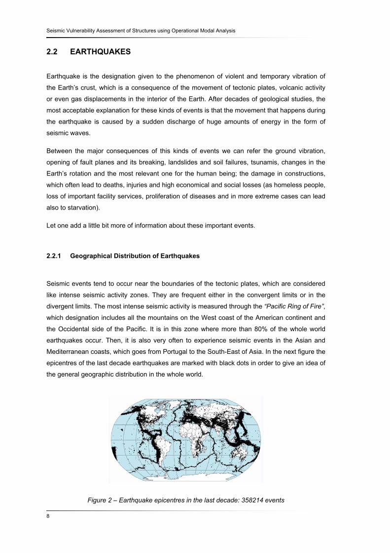
2.2.1 Geographical Distribution of Earthquakes
Seismic events tend to occur near the boundaries of the tectonic plates, which are considered
like intense seismic activity zones. They are frequent either in the convergent limits or in the
divergent limits. The most intense seismic activity is measured through the “Pacific Ring of Fire”,
which designation includes all the mountains on the West coast of the American continent and
the Occidental side of the Pacific. It is in this zone where more than 80% of the whole world
earthquakes occur. Then, it is also very often to experience seismic events in the Asian and
Mediterranean coasts, which goes from Portugal to the South-East of Asia. In the next figure the
epicentres of the last decade earthquakes are marked with black dots in order to give an idea of
the general geographic distribution in the whole world.
Figure 2 – Earthquake epicentres in the last decade: 358214 events

Seismic Vulnerability Assessment
9
The epicentre of an earthquake is the designation for the point of the Earth’s surface that is
directly above the point where the actual energy release is located. This last position is called
hypocentre.
The hypocentre or focus of an earthquake is actually the exact point in the interior of the Earth
where the release of energy through the form of wave happens. The deepest focuses were
registered at about 700 km of depth, associated to the subduction zone of South America’s
West coast.
Figure 3 – Epicentre and Hypocentre of an Earthquake
2.2.2 Types of Earthquakes
The major part of the earthquakes is related with the tectonic nature of the Earth, these kinds of
seismic events are designated of “Natural Earthquakes”. Though, there are also the
earthquakes caused by human actions. These last ones are called “Induced Earthquakes”. A
brief explanation of these two different types of earthquakes is described here.
2.2.2.1 Natural Earthquakes
The majority of seismic events are related with the tectonic nature of the Earth. The forces
involved in the tectonic of plates are applied in the lithosphere, which slides slowly over the
asthenosphere due to convection streams with origin in the mantle and in the core.
The plates can suffer different types of transformation depending on the direction of the natural
applied forces (see Figure 4, 5 and 6). They can separate themselves from each other (tension
forces), collide against each other (compression forces), or simply slide between them (torsion
forces). With the application of these kinds of forces the rocks will suffer some alterations until
they reach their elasticity point, from which it fails and suffers a sudden release of all the

Seismic Vulnerability Assessment of Structures using Operational Modal Analysis
10
accumulated energy during the process of elastic deformation. This energy, already said before,
is released by means of seismic waves which flood through the interior and surface of the Earth.
On the other hand, there is also the earthquake with volcanic origin. These kinds of events
happen due to the magma displacement inside the magma chamber or also because of the
pressure caused by the magma when it flows up to the surface.
Figure 4 - Divergent tectonic plates or normal fault
The tectonic plates separate from each other moving in opposite directions. When they move,
the material in the fusion state emerges to the surface through the fault creating a new oceanic
floor. The Meso-Atlantic and Meso-Pacific mountain ranges are a good example of this type of
plaque limits.
Figure 5 – Convergent tectonic plates or reverse (thrust) fault - Subduction phenomena
When the tectonic plates slide against each other, one has to climb over the other, creating an
elevation due to the type of junction that happens between the two plates. The junction zone
receives the name – subduction zone – and it can happen between two continental plates, one
continental and one oceanic plaque or between two oceanic plates. This kind of movement is
responsible for ¾ of the whole earthquakes in the world. The African and Euro-Asian tectonic
plates are an example of this case.

Seismic Vulnerability Assessment
11
Figure 6 – Lateral displacement between two tectonic plates – Strike-slip fault
In this last case the plates move transversally. The friction between plates is often very high and
big stresses can occur in this case. The rocks usually suffer big deformations, leading to high
levels of energy and hence, originating big earthquakes. The “Saint Andrews Fault” is an
example of this case.
2.2.2.2 Induced Earthquakes
Induced earthquakes, as the name refers, are directly or indirectly associated with the human
action. When one says human action, it can be due to big explosions (accidental or not),
collapse of big buildings, pression of the water in dams and even due to natural gas, mineral,
water or petroleum extractions. Although these kinds of events can cause significant levels of
vibrations (e.g. the 50 megatons nuclear bomb called “Bomba Tsar” released by URSS in 1961
produced vibrations equivalent to an M7 earthquake and its vibrations were registered in the
antipodal point of the Earth!), they cannot be compared with the natural ones, mainly because
they originate different records when comparing with the natural seismic records.
2.3 ANALYSIS PROCEDURES
Different types of approach can be used to define the dynamic characteristics of a structural
system. In the last few years, the main idea that a successful seismic behaviour would only be
accomplished if there was the possibility to control the level of local and global displacements of
the structure has been demystified. As this happens, new methods of seismic design for
structures started to evolve. Apart from the several existent methods, the following ones are the
most relevant and applicable to this subject.

Seismic Vulnerability Assessment of Structures using Operational Modal Analysis
12
2.3.1 Linear Elastic Analyses
The linear procedures should be applied only when dealing with regular buildings, i.e. with
nearly symmetric geometry. These kinds of analyses shouldn’t be performed on irregular
buildings unless they are capable to withstand the seismic actions in a nearly elastic manner
and the earthquake ductility demands are relatively low. In this field we make reference to the
following ones:
a) Equivalent Static Analysis
b) Dynamic Modal Analysis by Response Spectrum
2.3.2 Nonlinear Analyses
It is known that the loads suffered by a building during an earthquake usually make their
response to overpass the linear elastic range. This makes them undergo inelastic deformations
and local damage. Actually, the inelastic response is the mechanism that most helps the
structure to resist severe ground motion. Indeed, the yielding of structural elements contributes
for the capacity of the system to dissipate energy although a loss of resistance is often lost.
Bear in mind that parameters like the yield limit (fy) and the ductility ratio (μ) are very relevant for
these kinds of analyses.
In the nonlinear analysis domain one can use:
a) Nonlinear Static Procedure (NSP)
b) Nonlinear Dynamic Procedure (NDP)
In this present work it will be emphasised the nonlinear analysis, more specifically the nonlinear
static analysis, through the use of push-over analyses. The nonlinear static analysis, generally
designated as “push-over” analysis always consists in applying a loading to the system and
controlling the displacements that result from that loading. This approach appears to be a useful
tool for the study of nonlinear behaviour of structures and allow the engineer to know the
evolution of damage during the process. If the objective relies in reinforcing or repairing an
existent structure, this kind of approach will be of great utility.

Seismic Vulnerability Assessment
13
For this reason, in this field there have been some different approaches on how to design
structures and throughout the last years, some guidelines and methods have been developed.
Nevertheless the nonlinear dynamic analysis is the most accurate but also the most complex
when it comes to mathematical treatment of data due to unavoidable uncertainties. Notice that
this procedure will not be emphasised in this work once it goes out of the purpose of a simple
and expedite analysis.
2.3.2.1 Nonlinear Static Analysis
The present document concentrates itself in the nonlinear static analysis. The following
methods briefly described here are, in the present days, the most used in engineering
companies and the most reliable when it comes to the analysis of structural systems. In general
they rely on the following steps:
a) Definition of the resistant capacity of the structure through means of applied incremental
loadings or displacements. The outcome resistance/capacity of the system is usually
represented through a curve in a force-displacement plot.
b) Achieve the seismic behaviour critical points. “Performance Point” and “Target
Displacement”. These are defined through a correct definition of the seismic action and from the
nonlinear behaviour of the system.
c) Evaluation of the structural performance. This can be measured from the rotations,
displacements or stresses in some particular elements when one achieves the critical points of
seismic level pretended to simulate.
Within this domain, some references to the most usual methods are briefly described. Note that
in all of them the seismic behaviour is characterized by means of response spectrums.
Consequently, the structural system needs to be represented as a single degree of freedom
system.

Seismic Vulnerability Assessment of Structures using Operational Modal Analysis
14
- Displacement Coefficient Method (DCM):
In this method the final displacement is obtained through the structural capacity curve. The
elastic response is decreased affecting the elastic values by correction coefficients in order
to considerate the partial nonlinear behaviour. It is believable that the seismic performance
of a structure is easier to understand if the levels of local and global displacement are
recognized. In this perspective one can find the Push-Over Analysis, where the global
response of a structure is transformed in the response of an equivalent single degree of
freedom system. This specific method incorporates the adequate evaluation of the seismic
behaviour for different limit states and allows perceiving the evolution of yielding and
collapse on structural elements.
It is possible to find this kind of approach in NEHRP Guidelines for the Seismic Rehabilitation
of Buildings [FEMA-273, 1997], Pre-standard and Commentary for the Seismic Rehabilitation
of Buildings [FEMA-356, 2000] and recently in HAZUS-MH MR1 Technical Manual [FEMA,
2003] or Eurocode 8 [CEN, 2003].
- Capacity Spectrum Method (CSM):
The capacity spectrum method lets one know the exact point where the structural system
start to fail. In this process the seismic response point is obtained intersecting the capacity
curve of the structure with the seismic demands.
This kind of approach is further explained in ATC-40 [ATC, 1996].
- European Regulamentation – “N2” Method [CEN, 2003]
Based on inelastic spectrums this is a similar approach of the CSM method. The inelastic
response spectrum is obtained based on the elastic design spectrum by means of proper
reduction coefficients (Rμ) associated with the system ductility (μ). Though, it is also known
that this process has its disadvantages. It doesn’t consider energy dissipation characteristics
of the system and assumes “weak” relationships between ductile and elastic response of the
structural system. Though, it has been an integrated approach in recent versions of the
European Standards “Eurocodes”.

Seismic Vulnerability Assessment
15
2.3.2.1.1 Push-Over Analysis
As mentioned previously, the push-over analysis is included in the nonlinear static analysis
where it is used a displacement approach. This is a good option when it comes to the study of
dynamic behaviour of ordinary structures under seismic loads because most of them reveal a
nonlinear inelastic response to these kinds of inputs. Of course, these methods always require
mathematical techniques but when it comes to regular structures, i.e. symmetrical distribution of
masses, simplified procedures are given in some Codes or Technical Guides. Otherwise, it
turns out that the necessity to make use of sophisticated computer programs is imperative.
Anyway, the main issue lies in the input data; it is usually difficult to make use of correct
assumptions for this kind of values. That is why it is necessary that the engineer take advantage
of his know-how, making some acceptable simplifications. Then, with the results it is also
expected from him to look at them with extreme caution due to uncertainties that can’t be
mistreated.
The push-over static analysis comes in hand when dealing with multi-storey buildings because it
is based on a simple procedure. It allows the study of the nonlinear, post-yielding response of
the structure, by control of the displacement on the top of the building. It is a “lateral
displacement/base shear force” design procedure. The structure is analysed in the fundamental
mode and the lateral inertial seismic forces are vertically distributed accordingly. This step can
be done because the push-over procedures include the relation between the multi degree of
freedom structural system responses with a correspondent single degree of freedom model.
The forces are increased and the displacement is controlled on the top of the building. And the
building is assumed to reach an inelastic deformation.
Its main advantages are: it provides a tool to measure, in an approximate way, the plastic
deformation of the structure; and it is related to the expected deformation of the structure.
However, it has its limitations. The static push-over analysis is actually based on a linear system
for which the acceleration spectrum is elaborated. Also, the procedure is suitable for a building
whose seismic response is mainly in the fundamental mode. If the effect of higher modes is
introduced, the push-over analysis will increase its imperfection. Larger errors will be induced in
the results.

Seismic Vulnerability Assessment of Structures using Operational Modal Analysis
16
2.3.2.1.2 Fragility Curves
The concept of fragility curve will be used to evaluate the level of damage that a structure can
be into a determined damage state. The construction of these curves will be based on the
capacity of the building to resist horizontal forces by means of capacity curves which display the
spectral displacement in function of the spectral acceleration. Moreover, the fragility curves are
given by lognormal functions that will relate the probability of the building being in or exceeding
a certain level of seismic solicitation.
Fragility curves are often used in seismic engineering to describe the probability of reaching
different states of damage given a certain level of ground shaking.
For this concept a full chapter in this work is dedicated.

Operational Modal Analysis
17
3 Operational Modal Analysis
3.1 INTRODUCTION
The sophistication of the engineering software to project models and the evolution of the quality
of construction materials lead us to the ability of designing more resistant and lighter structures.
One important consequence of this evolution is the fact that it’s now necessary to control more
dynamic problems and vibration perturbances than before, which can often lead to fatigue and
noise disturbances. Operational Modal Analysis emerges as a valuable and powerful tool to
help engineers solve these kinds of problems.
The traditional modal analysis was first used around 1940 when engineers were trying to
understand the dynamic behaviour of an experimental airplane. In the late 1970’s and early
1980’s technical advances in equipment based on Fast Fourier Transform coupled with
personal computers modernisation propelled the interest of modal analysis as an analytical tool,
giving the opportunity to Operational Modal Analysis to rise. Operational Modal Analysis can
also be known by Output-Only Modal Analysis. The particular interest of this new enhancement
of modal analysis resides in the fact that testing is normally performed by just measuring the
responses of the structure under the operational or natural conditions, i.e. the system is excited
by natural or operational loads such as wind loads, wave loads, traffic loads, etc. If one wants to
test any structure in the laboratory, artificial loads are to be used applying some random tapping
on the structure. In Operational Modal Analysis forces are not recorded. Nevertheless, the
forces acting on a structure can still be estimated using the responses at several points together
with the Frequency Response Function (FRF) [Aenlle et. al., 2003].
These facts also led us to the chance of collecting and analyzing many channels of data
simultaneously, in a more expedite way and faster, which gave the experimentalist a whole new
way to understand and solve vibration and dynamic problems. Nowadays it is indispensable the
use of powerful tools when processing data in engineering studies. As this happens, the
Operational Modal Analysis is one, if not the best answer for these problems, providing the
possibility to understand the structural characteristics of complex structural systems in their
service conditions.

Seismic Vulnerability Assessment of Structures using Operational Modal Analysis
18
We can now develop accurate solutions for dynamic problems whether in design of new
structures or in rehabilitation of existing buildings.
3.2 APPLICATIONS OF OMA FOR STRUCTURAL IDENTIFICATION
Initially, in traditional input-output modal analysis, it was known the value for the forced dynamic
excitation applied to the structural system. In Operational Modal Analysis (OMA), more
specifically in Output-Only Modal Analysis, only the output variable is known, i.e. the dynamic
response. The advantage of using Operational Modal Analysis is that the dynamic responses
are obtained from natural excitation, such as ambient vibrations produced due to wind, traffic,
waves, etc. It is not necessary to use heavy excitation equipment to produce forced vibrations.
Operational Modal Analysis is the name given to the process where the modal parameters of a
structure are obtained using the vibration data captured with specific measurement devices
positioned in specific points of the structure. With this simple method it is possible to acquire
very useful information out of the structure about its physical properties such as masses,
stiffness and damping. Modal parameter estimation or curve fitting is the process of estimating
these parameters from experimental data. Furthermore, it can be shown that a set of modal
parameters completely characterizes the dynamic properties of any structure. This set of
parameter s is often called as modal model. Hence, the important modal parameters that
describe the dynamic properties of any structure are:
- The modal frequency, fn
- The modal configurations, Φn
- The damping ratio coefficients, ξn
In general, we can say that Operational Modal Analysis can cover a wide range of purposes and
it has been possible to clear some issues verified in the modulation of some linear systems. The
most relevant applications of OMA are:
- Model validation and updating:
The use of finite element models can be now validated and experimentally correlated. The
predictive analysis of constructed facilities becomes more and more important bringing this

Operational Modal Analysis
19
issue to the forefront. In this domain it is important to check the contribution of the non-structural
(or secondary) elements that usually interfere considerably in the stiffness of the structure (e.g.
masonry walls, adjacent buildings, etc…).
- Structural condition assessment and monitoring:
The assessment and monitoring of structural integrity and performance in the service state has
been enabled due to new developments in computer software, signal processing and
instrumentation technology. Makes possible to retrofit or reinforce particular zones of structures
that need to be repaired. For example in structures like: bridges, dams, off-shore platforms,
nuclear power plants, and so on…
- Load Estimation:
The loading of a structure can be estimated through the transfer matrix, which is obtained from
the modal properties that are known based on the modal analysis techniques. It’s a new and
innovative way of estimating loads on various kinds of structures.
- Soil-Structure interactions:
The analysis of the interaction between a structure, its foundations and the surrounding soil
medium has been significantly improved due to the new use of structural identification
techniques.
- Earthquake Engineering:
Structural identification is quite recent in this field of study though is starting to achieve an
important role due to its accurate measurements and results. Operational Modal Analysis can
be used to obtain accurate response models such that dynamic characteristics of large
structures and seismic capacities can be truthfully determined. It makes possible to achieve the
losses and level of damage in a structural system after an earthquake. It can also be used to
predict and build up hazard maps or shake-maps based on the levels of ground shaking
measured from the instrumented structures.

Seismic Vulnerability Assessment of Structures using Operational Modal Analysis
20
3.3 IDENTIFICATION TECHNIQUES
Mainly there are two different approaches to apply Operational Modal Analysis in real
structures. Ones are known for using directly measured data and the others also use measured
data but also the contribution of a parametric model.
3.3.1 Non-Parametric Techniques
In this type of technique, the modal parameters are estimated directly from measured data. With
these experimental values it is possible to build up the curves (e.g. frequency curves), functional
relationships or tables. Once the signal processing is done, the modal parameters are easily
obtained.
Figure 7 – Main steps in non-parametric technique methods
In this field the most common analysis methods are:
- Transient Analysis – usually applied when the system response is generated on the
basis of impulse (transient);
- Frequency Analysis – best application when the excitation is deterministic and either
periodic, or pseudo-random and periodic. The excitation is measured in time domain
and then transformed to frequency domain, making possible to obtain the frequency
response function which is the ratio between the response and excitation;
- Correlation Analysis – applied to stationary stochastically excited systems, the impulse
response function can be estimated from the response and from the correlation
functions of the excitation;
Experimental Data Signal Processing Modal Parameters
fn, ξn, Φn

Operational Modal Analysis
21
- Spectral Analysis – also useful when leading with stationary stochastically excited
systems.
In this kind of system identification, for the signal processing it is usually used techniques based
on Fourier transform algorithms, which will be further explained in the next subchapters.
Non-parametric models are traditionally associated with the Discrete Fourier Transform. They
are easier to use than the parametric techniques but also they have their limits. A traditional
non-parametric method for modal parameters estimation is the Basic Frequency Domain
method [Bendat et. al., 1993] based on the computation of auto and cross power spectra.
3.3.2 Parametric Techniques
When using a parametric technique, the modal parameters are estimated using a similar
method but this time with the addition of a parametric model. This model should be fitted to the
signal processed data (obtained by system identification) in order to obtain good parameter
estimation and then the desired modal parameters that characterize the dynamic response of
the real structure can finally be achieved.
Figure 8 – Main steps in parametric technique methods
Experimental Data
Signal Processing
Modal Parameters
fn, ξn, Φn
Parametric Model
Parameter
Estimation

Seismic Vulnerability Assessment of Structures using Operational Modal Analysis
22
When fitting the modal parameters it is often used one of these two techniques: Enhanced
Frequency Domain Decomposition (EFDD) as a simple fit or the Stochastic Subspace
Identification (SSI) which consists in a more advanced fit.
In practice, the parametric techniques using parametric models are available in the time and
frequency domain.
3.4 FREQUENCY DOMAIN DECOMPOSITION (FDD)
When using Operational Modal Analysis only the output of the system is known, i.e. the
response. This response can be expressed in displacement, velocity or acceleration and can be
referred to either time or frequency domain. Usually, most users are more comfortable when
working with responses given as accelerations in time domain.
Only in the field of Operational Modal Analysis the user can find a wide range of methods to
perform modal identification on structural systems.
Though, the modal parameters identification in the frequency domain can be performed by the
Frequency Domain Decomposition technique, from now on referred to as FDD, which is an
extension of the Basic Frequency Domain technique (BFD), also designated by simple peak
picking technique.
In this project, the author has chosen to focus on the FDD technique, where the use of Singular
Value Decomposition algorithm (SVD) is quite important, once it makes possible to estimate the
modal parameters.
When using FDD, one is partially taking advantage on direct peak picking eigenfrequencies
from the decomposition of the spectral density function matrix, and the response can be
separated into a set of single degree of freedom systems, each one corresponding to an
individual mode [Andersen et. al., 2000]. Inherently, one is fairly making use of U and S
matrices obtained with the SVD algorithm (for more information about this point consider
Appendix E) and the contemplation of white noise (where the spectral density function is
constant in a wide range of frequencies) is often necessary.
The principle in the FDD technique resides in the fact that any response can be written in modal
coordinates. It is necessary to integrate two times the acceleration output, ( )y t , in order to
obtain the correspondent displacement response in time domain, ( )y t .
1 1 2 2( ) ( ) ( ) ... ( ) . ( ) n ny t q t q t q t q tϕ ϕ ϕ= + + + =Φ (1)

Operational Modal Analysis
23
Once one has the responses in the time domain it is possible to calculate the covariance matrix
of the response, ( )yyC τ [Nielsen, 2000].
, ( ) ( ( ) ( ))( ( ) ( ))yi yj i yi j yjC E y t t y t tτ μ τ μ τ⎡ ⎤= − + − +⎣ ⎦ (2)
Note that when the index i is the same as j the designation auto applies to the correlation
function. If not, the term cross is used. The term [ ]E x refers to the expected value of x and
yμ to the mean value of the response.
The covariance function ( )yyC τ can also become the correlation function ( )yyR τ if the mean
value is zero and if the mean value, the variance and the standard deviation are all independent
of absolute time, i.e. when it corresponds to a stationary response [Newland, 1993]. If this
happens, the correlation function is given by:
, ( ) ( ) ( ( ))( ( ))yi yj yy i jR C E y t y tτ τ τ⎡ ⎤= = +⎣ ⎦ (3)
Alternatively, in the practical way of Operational Modal Analysis the covariance function is
obtained directly from the average values displayed in a number of time series, T.
0
1( ) ( ( ) ( ))T
yyC y t y t dtT
ω τ= +∫ (4)
Subsequently, if using the response equation into the covariance response matrix, we get
[Brincker et al., 2000]:
{ }
1 1 2 2( ) ( ) ( ) ... ( ) ( )
( ) ( ). ( )
n n
Tyy
y t q t q t q t q t
C E y t y t
ϕ ϕ ϕ
τ τ
⎧ = + + + = Φ⎪⎪ ⇒⎨⎪ = +⎪⎩

Seismic Vulnerability Assessment of Structures using Operational Modal Analysis
24
{ }( ) ( ). ( ) . . ( ). H H Hyy qqC E q t q t Cτ τ τ⇒ = Φ + Φ = Φ Φ (5)
Note that the ( )qqC τ matrix is almost diagonal, which leads us to the similarity with the Singular
Value Decomposition (SVD) equation:
( ) . ( ). . . T Tyy qqC C U S Uτ τ= Φ Φ ≈ (6)
The matrix U is a unitary matrix holding the singular vectors uij and S is a diagonal matrix
holding the scalar singular values Sij.
Afterwards, the transformation from time to frequency domain can be executed using the Fast
Fourier Transform (FTT) of the covariance function. Through this process, one is able to build
up the spectral density matrix, ( )yyS ω which will provide the user with all the information
related to the energy of the system.
These steps are briefly illustrated on Figure 9.
Figure 9 – Steps involved in the procedure from acceleration in time domain to power spectral
densities in frequency domain
The Fourier transform is based on the Fourier series expansion, which means that is only
applicable on periodic functions [Zill et. al., 2001]. As it is common, the response in time domain
is not periodic, but hopefully the covariance function of time response ( )yyC τ is. For this
reason, the Fast Fourier Transform (FFT) is performed on the auto covariance function and not
on the response itself [Newland, 1993].
( )y t ( )y t ( )yyS ω
FFT
( )yyC τ

Operational Modal Analysis
25
As this happens, with this consistent step one is able to obtain the response spectral density
matrix of modal coordinates ( )yyS ω , which can be defined by the following ways:
1( ) ( ).2
iyy yyS C e dωτω τ τ
π
+∞−
−∞
= ∫ [Nielsen, 2000] (7)
or
1( ) ( ). ( )*yyS y yN
ω ω ω= ∑ (8)
The previous equations are both recognized as Fourier Transforms of the covariance function,
{ }( )yyC τℑ . Special attention should be kept on the second alternative which corresponds to the
practical way of calculating spectral densities directly from time histories data, where N
corresponds to the number of available measurement series, ( )y ω to the Fourier Transform of
the time response series and * to its complex conjugate. This last equation allows obtaining an
average of spectral densities. This average approximation is automatically performed when one
uses the ARTeMIS Extractor to calculate the spectral density matrices out of each estimated
eigenfrequency (in Appendix F, a plot where all setups are demonstrated, Figures 66 to 72).
Particularly in OMA, this process is often adopted in a different but equivalent way:
( ) . ( ). Tyy qqS Sω ω=Φ Φ [Brincker et. al., 2000] (9)
Or in the matrix form, the same spectral density matrix can be expressed as:
1 1 1 2 1
2 1 2 2 2
1 2
, , ,
, , ,
, , ,
( ) ( ) ( )
( ) ( ) ( )( )
( ) ( ) ( )
n
n
n n n n
y y y y y y
y y y y y yyy
y y y y y y
S S S
S S SS
S S S
ω ω ω
ω ω ωω
ω ω ω
⎡ ⎤⎢ ⎥⎢ ⎥= ⎢ ⎥⎢ ⎥⎢ ⎥⎣ ⎦…
(10)

Seismic Vulnerability Assessment of Structures using Operational Modal Analysis
26
From the previous equation, since the modal coordinates are un-correlated, the power spectral
density matrix ( )qqS ω of the modal coordinates is diagonal. This operation results in a Singular
Value Decomposition of the response spectral matrix ( )yyS ω since the mode shapes are
orthogonal. The elements in the diagonal are estimates of the auto spectral densities , ( )yi yiS ω
and the elements out of the diagonal of the matrix are estimates of the cross spectral densities,
, ( )yi yjS ω .
Hence, if we have a multiple loading case (e.g. natural load as the wind which acts in different
points of the structure simultaneously), then the spectral matrix can reach the full rank (the
necessary rank is the largest number of closely spaced modes plus the number of independent
noise sources) and the singular values obtained will give good results for the auto spectral
density functions of the single degree of freedom systems corresponding to each of the modes
[Brincker et. al., 2000].
Some of the advantages that can be identified when using Frequency Domain Decomposition
techniques are:
- Once you have the data (preferentially with natural/multiple input loads), it is very easy
to use and identify the different modes immediately.
- Having the plot of the power spectral densities, it is easy to pick at any frequency and
any singular value, allowing a better understanding of the structural behaviour.
On the other side, there are also some sceptical perspectives about this approach which state
that:
- It is impossible to estimate damping
- Frequency resolution is no better than line spacing
A review of the most commonly used methods of modal identification used in civil engineering
applications can also be found in reference [Cunha, 2005]

Operational Modal Analysis
27
3.5 CASE STUDY – LABORATORY MODEL
This chapter is focused on the analysis of the ambient vibration data acquisition of a reduced
model constructed on purpose for this investigation, in the laboratory of Civil Engineering of
Aalborg University. The purpose here is to simply illustrate how Operational Modal Analysis can
be performed, specifically using FDD techniques. Successively, the results obtained using this
method to identify the modal characteristics of the model are presented and described.
3.5.1 Description of the Laboratory Model
The lab model used in this study was built on purpose for this project. It is expected to
reproduce the behaviour of a common concrete frame building of three stories.
The model is 1,00 meter height, 0,31 meters between each storey, the storey panels have 0,02
meters of thickness and the columns are simple round steel bars with approximately 0,01
meters of diameter.
In Figure 10 it is illustrated a simple sketch of the lab model and in Figure 11 a picture of the
real model can be previewed.
Figure 10 – Simple sketch of the reduced lab model and its nodes

Seismic Vulnerability Assessment of Structures using Operational Modal Analysis
28
Figure 11 – Perspective view of the real laboratory model and accelerometers detail
3.5.2 Data Processing and Modal Identification Procedures
The responses of the building model to the ambient vibration tests were carried out using 6-
channel data acquisition system measured at selected points with Miniature DeltaTron TEDS
from Brüel & Kjær (see Figure 12). These accelerometers were placed in the desired spots with
natural bee wax. A schematic diagram of the sensors layout is then shown in Figure 13 where
all the channels can be identified.
Figure 12 – Brüel & Kjær accelerometers (Miniature DeltaTron TEDS) used in the model
ambient test
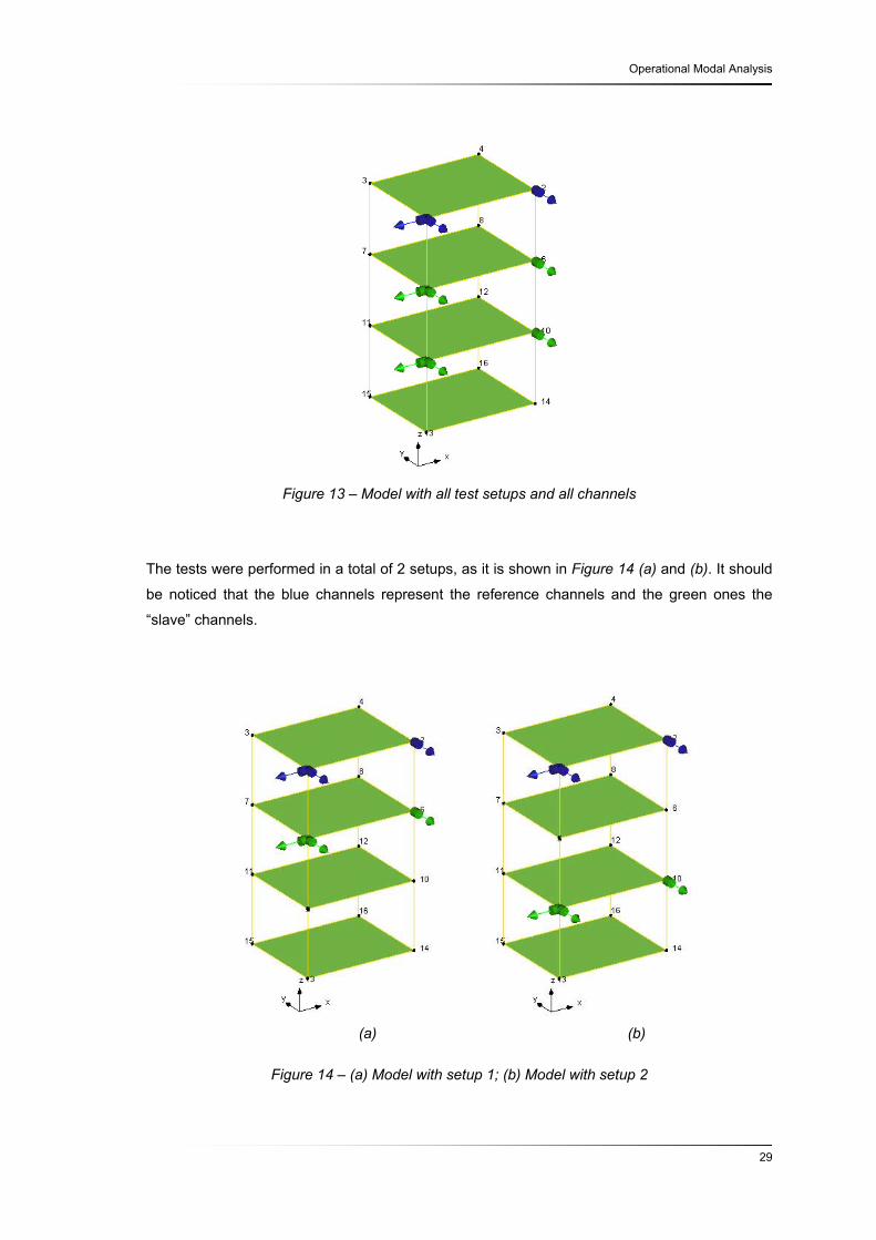
Operational Modal Analysis
29
Figure 13 – Model with all test setups and all channels
The tests were performed in a total of 2 setups, as it is shown in Figure 14 (a) and (b). It should
be noticed that the blue channels represent the reference channels and the green ones the
“slave” channels.
(a) (b)
Figure 14 – (a) Model with setup 1; (b) Model with setup 2

Seismic Vulnerability Assessment of Structures using Operational Modal Analysis
30
For each channel and for each setup, the acceleration-time histories were recorded for 60
seconds. The data, originally sampled at 1500 Hz, resulted in a number of samples of 90000
data points for each setup. Decimating the data 10 times the sampling frequency decreased to
150 Hz and the Nyquist frequency was then 75 Hz.
Certain particularities of the study case must be taken into account before processing the data.
Firstly, the ambient vibration tests were performed in the laboratory and as this case refers to a
reduced model, the input had to be taken by means of slightly tapping the structure on the sides
of the storey panels.
In order to process the data, the ARTeMIS Extractor v4.0 [SVIBS] software package was used.
In particular the FDD method. The singular values obtained from the spectral density matrix are
shown in Figure 15.
Figure 15 – Singular values of spectral density matrices
As one can see in the previous figure, there are some close modes. These were not found
immediately. The first frequency resolution (i.e. number of frequency lines) used was 1024. This
fact led to an excessive detail in the curves of the singular values. Furthermore, it was making
difficult to find reasonable mode shapes, especially the close ones. If one wanted a better
estimation, the other available method in the software, such as Stochastic Subspace
Identification (SSI) could be a good alternative. Though, once in this project it is only mentioned
the FDD technique, the alternative was found in changing the frequency resolution to 256

Operational Modal Analysis
31
frequency lines. This modification led to a higher average in the singular values which made
possible an easier finding of close modes when doing the peak picking.
As this chapter has the objective to simply illustrate how OMA can be done, one will only stick to
the first nine modes of the structure. In addition, further attention in higher modes is not that
important for the estimation of the modal characteristics of the structure. As this happens, in
Table 22 the frequency values are shown.
Mode # Frequency [Hz]
1 10,84
2 11,13
3 16,11
4 32,52
5 32,81
6 48,05
7 49,51
8 49,80
9 73,83
Table 1 – Frequency values for each mode
As well as in Figure 16, 17 and 18 the fundamental, the second and third order mode shapes
are presented, respectively.
Figure 16 – 1st, 2nd and 3rd mode shapes of the reduced model

Seismic Vulnerability Assessment of Structures using Operational Modal Analysis
32
Figure 17 – 4th, 5th and 6th mode shapes of the reduced model
Figure 18 – 7th, 8th and 9th mode shapes of the reduced model

Fragility Curves
33
4 Fragility Curves
4.1 SCOPE
In this chapter it is described the method adopted to estimate the damage in a structural
system. Will be developed functions for estimating building damage using the guidelines
provided by FEMA – “HAZUS-MH MR1 Technical Manual” [FEMA, 2003]. These guidelines are
the result of a project conducted for the National Institute of Building Science (NIBS) under a
cooperative agreement with the Federal Emergency Management Agency (FEMA) and they
constitute a good method for the evaluation of damage in buildings.
It is important to refer that this method is oriented to the American type of construction and to
the American seismic region codes. Anyway, the adjustment for the European standard will be
taken into account with the adequate choice of the building type and the response spectrum of
the zone where the building will be considered.
Actually, most buildings are designed using linear-elastic analysis methods. This happens due
to their simplicity when compared with more complex, nonlinear methods. Frequently, the basis
earthquake building response design is based on linear-elastic properties of the structure
reduced by means of reduction coefficients which take into account nonlinearities, where one
can include the damping ratio. This reduction factor (also known as “R factor”) is often based on
empirical data where the account for the ductility of the structural system, redundancy,
overstrength and other factors that influence the building’s capacity is made. It is important to
consider that although this kind of approach and methods are difficult to justify by rational
engineering analysis, they are also reasonably successful when regarding to the performance of
some buildings in past earthquakes. Though, the building capacity estimation can always be
improved. Latter acknowledgements recognise that building damage is primarily a function of
building’s displacement rather than force.
For this reason, in this project, a different approach is adopted. Ambitiously, successful
prediction of a structure capacity and response in the inelastic range will probably lead to more
accurate results in the damage estimation of the system after an earthquake. In this chapter it is
performed an estimation of the structure’s capacity by means of push-over curves. These
curves, combined with capacity spectrum method (CSM) techniques [Mahaney et. al., 1993]

Seismic Vulnerability Assessment of Structures using Operational Modal Analysis
34
and [Kircher, 1996] will provide simple and accurate ways of predicting inelastic building
displacement responses for damage estimation purposes.
4.2 PROCEDURE
The inbuilt process required to estimate essential facility damage using capacity and fragility
curves include the following fundamental steps:
- Classification of the model building type according to HAZUS;
- Definition of the seismic design level that represents the essential facility of interest
according to HAZUS;
- Construction of the Capacity Curve;
- Construction of the Fragility Curves;
- Definition of the Response Spectrum at the building’s site according to Eurocode 8;
- Definition of the Solicitation Spectrum;
- Estimation of the structural system’s response;
- Quantification of discrete probabilities of structural damage for each damage state.
In the first step, according to the HAZUS methodology it is necessary to include the structural
system in study in one of the categories defined by these guidelines in order to proceed in
accordance to the rest of the procedure.
Secondly, it is also necessary to define the level of seismic design taken into account when the
construction of the structure was made.
Then, the estimation of the capacity of the structural system is made by means of capacity
curves. These curves, combined with the demand spectrum at the building’s site will define the
peak spectral response, for a certain level of ground shaking. These values will be presented by
means of spectral displacements and spectral accelerations (ADRS – Acceleration-
Displacement Response Spectra).
Afterwards, the fragility curves (lognormal functions) will give us an estimate of the cumulative
probability of the structure being in, or exceeding each damage state for the given level of
ground shaking (or ground failure). Cumulative damage probabilities are differenced to create

Fragility Curves
35
discrete damage state probabilities. Discrete probabilities of damage are used directly as inputs
to induced physical damage and direct economic and social loss modules.
For this to happen, the definition of the response and solicitation spectra has to be carried out.
These spectra are based under the assumptions recognized in Eurocode 8 and specifically for
the seismic zone of Portugal.
Subsequently the intersection between the capacity curve and the solicitation spectrum is
reached. With this step the peak spectral displacement response is achieved.
Crossing the peak spectral displacement response value with the fragility curve will be the last
step of the procedure. Hence, discrete probabilities will be presented to quantify the structural
damage for each damage state given a certain spectral displacement.
4.3 CASE STUDY
4.3.1 Model Description
It is used a very simple model. It was chosen a concrete structural frame with one storey as we
can see in the next figure. The cross section of the columns has 50x50 cm and the cross
section of the beams has 60x50 cm. It is a double-symmetrical structure with 8 meters length on
the side and 6 meters of height. The foundations are assumed to restrain all movements and
rotations.
Figure 19 – Simple concrete frame structure adopted [SAP2000 v10]

Seismic Vulnerability Assessment of Structures using Operational Modal Analysis
36
4.3.2 Model Building Type Classification
Between the sixteen classes defined by HAZUS methodology, the “C1L” category is the one
chosen to illustrate the proposed example of a simple frame structure.
This category represents a low-rise reinforced concrete moment resistant frame structure (C1).
Because the proposed model is supposed to be as simple as possible, one has assumed only
one storey, like a low-rise building (L). The non-structural elements weren’t considered at all
although in practical cases one knows that they would contribute significantly to raise the
stiffness values and the resistance of the structure to lateral forces.
4.3.3 Building Damage States (C1L)
According to HAZUS, the methods of damage estimation in structures are directly correlated
with the building type and with the level of ground shaking. They are well defined for each
building type. A brief description of the damage occurred in the structural elements can be
found in these guidelines. Furthermore, if a detailed approach needs to be done, there is also
reference to the effects suffered by the non-structural elements.
As one knows, the level of damage increases continuously accordingly with the level of shaking
or earthquake demand. Though, it is not very practical to describe it with a continuous scale.
Subsequently, these ranges of damage assumed here are used to describe the level of damage
in four different states, providing all the information about the buildings physical condition.
This method separates different levels of damage in: None, Slight, Moderate, Extensive and
Complete Structural Damage.
The loss functions related to these five levels of damage are based on various loss parameters,
such as economic losses, casualties and loss of functionality in service conditions, though in
this project the final intention is only to estimate the loss of accuracy in the results obtained for
damage estimation in the structure for a general perspective of an earthquake scenario.
The predicted values that outcome from this physical damage estimation method are then
transformed in terms of the probability of a structure being in any of the five damage states.
For the proposed structure (C1L) the damage states are described as follows:
No Structural Damage: No damage detected on the structure;
Slight Structural Damage: Flexural or shear type hairline cracks in some beams and columns
near joints or within joints;

Fragility Curves
37
Moderate Structural Damage: Most beams and columns exhibit hairline cracks. In ductile frames
some of the frame elements have reached yield capacity indicated by larger flexural cracks and
some concrete spalling. Nonductile frames may exhibit larger shear cracks and spalding;
Extensive Structural Damage: Some of the frame elements have reached their ultimate capacity
indicated in ductile frames by large flexural cracks, spalled concrete and buckled main
reinforcement; Nonductile frame elements may have suffered shear failures or bond failures at
reinforcement splices, or broken ties or buckled main reinforcement in columns which may
result in partial collapse;
Complete Structural Damage: Structure is collapsed or in imminent danger of collapse due to
brittle failure of Nonductile frame elements or loss of frame stability.
Approximately 13% (in low rise structures) of the total area of C1 buildings with complete
damage is expected to be collapsed.
4.3.4 Seismic Design Level
The capacity and fragility curves that are about to be built here to estimate probability of Slight,
Moderate, Extensive and Complete damage in general structures are referred to a building
which seismic design level is known. The seismic standards assumed in this method (HAZUS)
are High-Code, Moderate-Code, Low-Code or Pre-Code standards (this last one applies to
structures which are not seismically designed). This means that this methodology permits the
user to select the seismic design level considered appropriate for the structure in study and for
the region where it is located.
As this happens, the engineer is able to choose which design level fits best his very own case of
study. For example, in areas with a high seismicity (e.g. Azores), important service buildings of
newer construction are best represented by High-Code standards (i.e. damage functions). On
the other hand, for buildings constructed before the existence of such codes (before 1940),
which were not designed for earthquake loads, should be modelled regarding the Pre-Code
design level.
In this present document, as one is dealing with a very simple structure, the seismic design
code admitted will be the Pre-Code one. This option will provide the worst approach that can be
done, being at the same time in the conservative side assuming that it was not made any
seismic consideration regarding the conception of the present frame structure.

Seismic Vulnerability Assessment of Structures using Operational Modal Analysis
38
4.3.5 Push-Over Curve to Capacity Curve
The structural system’s push-over curve is a force-deflection plot which displays the lateral load
resistance of the building as a function of its lateral displacement (e.g. base shear as a function
of the displacement on the top of the structure). Making use of this plot in order to obtain an
estimate of the real building displacement response and easily compare with earthquake
demands (overlaying the capacity curve with a response spectrum) is a possible and
reasonable estimation of the buildings capacity. Furthermore, the capacity curve of the same
structure can be obtained. For this, the push-over plot should be normalized, i.e. the force axis
should be converted to spectral acceleration and the displacement axis to spectral
displacement. This operation, where spectral coordinates are calculated (displacement and
acceleration), makes use of the elastic period of the structure and the effective modal mass and
effective modal height, which are always correlated with the first mode shape of the structure,
the fundamental mode shape.
The construction of these curves implies the definition of, at least, three important points in the
progress of the capacity response of the structure:
- Design Capacity (Dd, Ad)
- Yield Capacity (Dy, Ay)
- Ultimate Capacity (Du, Au)
Figure 20 – Capacity Curve

Fragility Curves
39
As it can be seen in Figure 20, from the origin until the yielding point of the structure, the
capacity curve is assumed to be linear with stiffness based on an estimate of the structure’s true
(elastic) period. Note that this “true” period is often longer than the period obtained from the
“Codes” due to the existence of flexural cracking in the concrete or masonry elements, flexing
diaphragms, flexibility of foundations and some other factors that can also affect the real
stiffness of the structure.
From the yield point up to the ultimate point, the capacity curve gradually transits from a purely
elastic state to a fully plastic state, gradually loosing its resistance.
Finally, although the capacity of deforming without loss of stability of a certain building goes a
little bit beyond its ultimate state, its structural system provides no additional resistance to
lateral forces (as the earthquake forces). This is the main reason why after the ultimate point it
is assumed a linear horizontal line in the plot.
In accordance to “HAZUS-MH MR1 Technical Manual” [FEMA, 2003], the capacity is built based
on some engineering properties that associate the design, yielding and ultimate capacities of
the structure for the assumed building type. These properties are defined by the following
parameters:
Cs, design strength coefficient (fraction of building’s weight) [-];
eT , true elastic period of the structure in the fundamental mode [s];
1α , fraction of building effective weight [-];
2α , fraction of building effective height [-];
γ , “overstrength” factor relating yielding strength and design strength [-];
λ , “overstrength” factor relating ultimate strength and yielding strength [-];
μ , ductility factor relating ultimate displacement with μ times the yield
displacement [-].

Seismic Vulnerability Assessment of Structures using Operational Modal Analysis
40
Although all these values can be taken from the guidelines, the parameters 1α and 2α can be
confirmed manually from the following equations:
11
1
N
ii
M
mα
=
=
∑ (11); 1
2top
HH
α = (12)
2
1
2
1
.[ ]
.
N
j jnj
n N
j jnj
mM kg
m
=
=
⎛ ⎞Φ⎜ ⎟
⎝ ⎠=Φ
∑
∑ (13)
1
1
. .[ ]
.
N
j j jnj
n N
j jnj
H mH m
m
=
=
⎛ ⎞Φ⎜ ⎟
⎝ ⎠=Φ
∑
∑ (14)
Where 1M represents the effective modal mass and 1H the effective modal height. Once
again, one reminds the reader that these parameters constitute a good approximation method
and intend to represent a multi-degree of freedom system as a simple single degree of freedom
system. This concept is illustrated on the next figure.
Figure 21 – From a MDOF system to a SDOF system

Fragility Curves
41
On the next pages, the construction of the capacity and fragility curves, within certain
assumptions, will be performed. Moreover, also the intersection of the capacity curve of the
structure with the solicitation spectrum of the seismic action will be achieved. This process will
allow the possibility to estimate damage probability of the structure being or exceeding a certain
damage state.
4.3.6 Fragility Curves
Fragility curves are defined according to the four limit states already referred: Slight, Moderate,
Extensive and Complete. These curves are lognormal functions that correlate the probability of
exceeding or being in a certain limit state for a certain level of seismic solicitation. These curves
can be estimated through different parameters: for ground failure – Peak Ground Displacement
(PGD); for ground shaking – Peak Spectral Response (PSR) either in displacement or
acceleration; for lifeline facilities – Peak Ground Accelerations (PGA). For this present case, the
ground shaking parameter seems the most appropriate and as this happens, one will focus on
the peak spectral response, that is to say in the spectral displacement, dS .
Characterized by median and lognormal standard deviation, these curves are hardly influenced
by the level of ground excitation and by the variability associated to a certain limit state.
Hence, the probability of being or exceeding a certain limit state, for a certain spectral
displacement value, dS , is modelled according to the following cumulative lognormal
distribution:
,
1( | ) .ln dd
d dsds
SP ds SSβ
⎡ ⎤⎛ ⎞= Φ ⎢ ⎥⎜ ⎟
⎝ ⎠⎣ ⎦ (15)
where, Φ is the standard normal cumulative distribution function;
ds is the structural damage state;
dS is the spectral displacement;
,d dsS is the median value of spectral displacement at which the building
reaches the threshold of the damage state;
dsβ is the standard deviation of the natural logarithm of spectral
displacement of damage state.

Seismic Vulnerability Assessment of Structures using Operational Modal Analysis
42
4.3.7 Elastic Response Spectrum
In order to predict the seismic response of the structure, the seismic response spectrum
adopted is defined in EC8 [CEN, 2003]. For this case, it is calibrated for the region of Lisbon in
Portugal (Type 1 seismic action). This spectrum was chosen just for illustration purposes and it
can not be always considered the most dangerous for every situations of ground motion. The
seismic action is characterized by a normalized elastic response spectrum where the
acceleration is a function of the period of the structure. For a damping rate of 5% (assumed by
the author for the linear response of the structural system) the following expressions define the
adopted spectrum [CEN, 2003]:
0( ) . . 1 .( 1) 0 , if e g BB
TS T a S T TT
ηβ⎡ ⎤
= + − ≤ ≤⎢ ⎥⎣ ⎦
(16)
0( ) . . , if e g B CS T a S T T Tηβ= ≤ ≤ (17)
0( ) . .k1
. , if Ce g C D
TS T a S T T TT
ηβ ⎡ ⎤= ≤ ≤⎢ ⎥⎣ ⎦ (18)
0( ) . .k1 k2
. . , if C De g D
D
T TS T a S T TT T
ηβ⎡ ⎤ ⎡ ⎤= ≥⎢ ⎥ ⎢ ⎥⎣ ⎦⎣ ⎦
(19)
where, ( )eS T Elastic spectrum ordinate [m/s2]
T Period of a linear single degree of freedom system [s]
0β Amplification coefficient of spectral acceleration for 5%ξ = (assumed
damping ratio)
,B CT T Constant spectral acceleration zone limits [s]
DT Constant spectral displacement initial value [s]
1 2,k k Exponential parameters that have influence on the spectra for values of
vibration higher than e C DT T , respectively.
S Soil class parameter

Fragility Curves
43
η Correction coefficient for the viscous damping (for 5% of viscous
damping, 5%η = )
ga Design value for the maximum nominal acceleration on the base of the
system for the reference return period. Considering a Type B soil (stiff
deposits of sand, gravel or over-consolidated clay with considerable
depth of at least 10 meters), a seismic action of Type 1 and taking into
account the zone of the city of Lisbon (Zone 1), the value of ga =1,7
m/s2 [Campos Costa, 2007].
As this spectrum comes as a plot of period-spectral acceleration it is necessary to represent it
as a plot of spectral displacement-spectral acceleration (ADRS format – Acceleration-
Displacement Response Spectra) in order to cross it with the capacity curve of the building and
by this way achieve the approximate response of the structure.
For this reason, the spectral displacement is obtained from:
2
.2d aTS Sπ
⎛ ⎞= ⎜ ⎟⎝ ⎠
(20)
where, dS is the Spectral displacement [m]
aS is the Spectral acceleration [m/s2]
T is the Period [s]
4.3.8 Solicitation Spectrum
In order to take into account the fact that the structure can be pushed beyond its elastic limits,
one should take into account not only the linear viscous damping but also the energy dissipated
during the hysteretic cycles. Hence, modifications on the elastic response spectrum have to be
performed in order to achieve the solicitation spectrum (or effective damped spectrum).

Seismic Vulnerability Assessment of Structures using Operational Modal Analysis
44
This can be done with the use of an effective viscous damping coefficient (higher than 5%)
which is given by the following expression:
.eff E H Kξ ξ ξ= + (21)
where, effξ is the effective damping coefficient [%]
Eξ is the elastic (pre-yield) damping coefficient [%]
Hξ is the hysteretic damping coefficient [%]
K is a degradation factor that defines the effective amount of hysteretic
damping as a function of earthquake duration, as specified in Table 1.
Degradation Factor (K)
Short Moderate Long
0,4 0,2 0
Table 2 – Degradation factor for the effective damping of a C1L building model with a Pre-Code
design
The hysteretic damping coefficient Hξ will depend on the amplitude of the response and on the
area defined by the hysteretic cycle on a spectral displacement-spectral acceleration plot.
Hence, in order to estimate this parameter, a bilinear representation of the capacity curve must
be done previously. Attention must be done to the fact that the area delimitated by the two lines
must be exactly the same as the area delimitated by the capacity curve itself. This guarantees
the same energy involved in the process. With this representation it is possible to estimate the
value of the delimited area of the hysteretic cycle, DE . This area is calculated based on the
next formula:
4 ( . . )D i iE a D d A= × − [m2/s2] (22)

Fragility Curves
45
Subsequently, the hysteretic coefficient can be calculated through [Candeias, 2000]:
50 ..D
HED A
ξπ
= [%] (23)
where, D is the peak displacement response on the capacity curve
A is the correspondent peak acceleration response
Once the effective damping coefficient value is achieved for the desired model, modifications
can be made on the elastic solicitation spectra calculated according to Eurocode 8, but now
where 1η ≠ and 5%ξ ≠ . By this way, the response spectrum can be reduced to an effective
damping reduction coefficient (η ) given by:
7 0,72 eff
ηξ
= ≥+
(24)
On the following pages, all the calculations are performed and the respective plots presented.
4.3.9 Probability of Damage
Finally it is possible to achieve the desired estimations of the damage encountered in the
model. This last step consists in crossing the data (the two curves) of the capacity curve of the
model with the solicitation spectrum of the zone in study for the same model.
By this way, one can obtain the spectral displacement and acceleration coordinates for the peak
response of the structural system ( ,dr arS S ).
The spectral displacement drS of the peak response of the building is then the important
parameter to characterize the probability of the level of structural damage.

Seismic Vulnerability Assessment of Structures using Operational Modal Analysis
46
Additionally, the discrete probabilities associated with each level of damage are given by:
( ) 1 ( )
( ) ( ) ( )
( ) ( ) ( )
( ) ( ) ( )
( ) ( )
P ds None P ds Slight
P ds Slight P ds Slight P ds Moderate
P ds Moderate P ds Moderate P ds Extensive
P ds Extensive P ds Extensive P ds Complete
P ds Complete P ds Complete
= = − ≥
= = ≥ − ≥
= = ≥ − ≥
= = ≥ − ≥
= = ≥

Fragility Curves
47
4.3.10 Procedure according to HAZUS:
4.3.10.1 Capacity Curve
In this first approach for the present structure, the following values obtained from “HAZUS-MH
MR1 Technical Manual” [FEMA, 2003] were used to build up the capacity curve and admitted as
the following:
Building Type Cs [-] Te (s) α1 [-] α2 [-] ɣ [-] λ [-] μ [-]
C1L 0,033 0,40 1,00* 1,00* 1,50 2,25 5,00 Table 3 – Code building capacity parameters: Design Strength (Cs), Period (Te), Push-Over
Mode Response Factors (α1, α2), Overstrength Ratios (ɣ, λ) and Ductility Factor (μ)
for the C1L building type and for Pre-Code Seismic Design
*Note that for the effective modal weight and height coefficients the value was not adopted from
the HAZUS tables once for this example, where the frame structure has uniquely one storey,
the effective mass ( 1α ) or height ( 2α ) coefficients will actually be exactly the same as the real
one. The system does not need to be reduced to one degree of freedom.
It is also relevant to refer that all the values presented in the HAZUS Guideline’s tables are
referred to a frame structure of 20 m height. Because of this fact, the appropriate reduction to 6
m height was performed to obtain more adequate parameters for the present case of study.
Starting from the values assumed previously, it is now possible to estimate the spectral
displacements and accelerations correspondent to the yielding and ultimate capacity points.
These points are obtained through the following expressions:
- Yielding Capacity Point:
29,8y y eD A T= × × [m] (25)
1
sy
CA γα×
= [m/s2] (26)

Seismic Vulnerability Assessment of Structures using Operational Modal Analysis
48
- Ultimate Capacity Point:
u yD D λ μ= × × [m] (27)
u yA A λ= × [m/s2] (28)
Thus, the values obtained for the present case are presented in the next table.
D [m] A [m/s2]
Yielding Capacity 0,002 0,495
Ultimate Capacity 0,022 1,114 Table 4 – Spectral displacements and spectral accelerations for the yielding and ultimate
capacity points
And the correspondent capacity curve plot is represented underneath:
Capacity Curve
0
0,2
0,4
0,6
0,8
1
1,2
0 0,01 0,02 0,03 0,04 0,05 0,06
Spectral Displacement [m]
Spec
tral
Acc
eler
atio
n [m
/s
2
]
Figure 22 – Capacity Curve for C1L building type under the Pre-Code seismic design level

Fragility Curves
49
4.3.10.2 Fragility Curves
HAZUS methodology provides the median DSSd and the standard deviation DSβ values for
each building type and for each level of seismic design. These assumed values are presented
in Table 5.9d (in inches) in HAZUS-MH MR1 Technical Manual [FEMA, 2003]. The
correspondent correlation to meters has been performed.
For this present case, as the first approach intends to follow as much as possible the method
prescribed by the guidelines adopted, the following values presented in Table 4 were taken into
account.
Damage State Slight Moderate Extensive Complete
DSSd [m] 0,0183 0,0292 0,0732 0,1829
DSβ 0,98 0,94 0,90 0,97
Table 5 – Fragility Curve Probabilistic Parameters for a C1L building type
Hence, the fragility curves can be plotted as presented in Figure 23.
Figure 23 – Fragility Curves for a C1L building type with Pre-Code seismic design

Seismic Vulnerability Assessment of Structures using Operational Modal Analysis
50
4.3.10.3 Response Spectrum
According to the elastic response spectrum built having in mind the standard rules from EC8
[CEN, 2003], the following values were adopted to create the normalised response spectrum.
For this case, and because it is just a mere illustration of the process, one can acknowledge
some assumptions. As this happens, the values in the next table are related to a structure
planted in a soil of class B with a viscous damping rate of 5% (according to EC8 [CEN, 2003]).
Eurocode Parameters for Spectral Response, 5%ξ = , Class B soil
S 0β k1 k2 BT CT DT ga η
1,35 2,5 1 2 0,1 0,25 2 1,7 1
Table 6 – Elastic spectral response parameters according to Eurocode 8
Hence, the correspondent response spectrum obtained is presented in Figure 24.
0
1
2
3
4
5
6
7
0 1 2 3 4 5 6 7 8
T [s]
S a [m
/s 2 ]
Figure 24 – Normalised Response Spectrum in Period-Spectral Acceleration, 5% damping, Soil
Class B

Fragility Curves
51
The same spectrum can also be represented in spectral coordinates, ,d aS S .
0
1
2
3
4
5
6
7
0 0,01 0,02 0,03 0,04 0,05 0,06 0,07 0,08
Sd [m]
S a [m
/s 2
]
1
Figure 25 – Normalised Response Spectrum in Spectral Displacement-Spectral Acceleration,
5% damping, Soil Class B
4.3.10.4 Solicitation Spectrum
To obtain the solicitation spectrum, it is necessary to calculate the effective damping as it was
seen before.
The elastic damping is assumed as 5% for the elastic range. The hysteretic damping coefficient
implies the estimation of the hysteretic cycles and the bilinear representation of the capacity
curve.
Figure 26 – Bilinear representation of the capacity curve

Seismic Vulnerability Assessment of Structures using Operational Modal Analysis
52
With this representation it is also possible to approximately represent the hysteretic cycle.
Figure 27 – Approximate Hysteretic Diagram representation
Therefore, the damping coefficients for each of the durations were estimated.
Duration Short Moderate Long
ξE 5
ξH 40,699
K 0,4 0,2 0
ξeff 21,28 13,14 5,00
Table 7 – Effective damping for different soil excitation durations
Furthermore, the reduction coefficients based on the effective damping are presented in the
following table:
Duration Short Moderate Long η 0,7 0,7 1
Table 8 – Reduction factor for the elastic response spectrum for different soil excitation
durations

Fragility Curves
53
As a result, one can notice that for short and moderate seismic action durations the solicitation
spectrums will be the same. This happens due to the imposition of 0,7η ≥ .
In Figure 28 the resultant solicitation spectrums are presented (Response Spectrum and
Damped Solicitation Spectrums).
0
1
2
3
4
5
6
7
0 0,01 0,02 0,03 0,04 0,05 0,06 0,07 0,08
Sd [m]
S a [m
/s 2 ]
1
Response Spectrum
Solicitation Spectrum (Short & Moderate)
Solicitation Spectrum (Long)
Figure 28 – Response and solicitation spectrums (according to EC8)
4.3.10.5 Structural Response Estimation
For this step, only the short and moderate durations were taken into account for the
determination of the peak spectral point. This is because in this work one just wants to illustrate
the proceedings. As this happens, repeating the same process for the long solicitation spectrum
would give different results but the method would be exactly the same.
Hence, the intersection between the capacity curve and the short (and moderate) solicitation
spectrum is presented in Figure 29, which provides the user with the coordinates of the model
response.

Seismic Vulnerability Assessment of Structures using Operational Modal Analysis
54
0
1
2
3
4
5
6
7
0 0,01 0,02 0,03 0,04 0,05 0,06 0,07 0,08
Sd [m]
S a [m
/s 2 ]
1
Response Spectrum
Solicitation Spectrum (Short & Moderate)
Capacity Curve
Figure 29 – C1L model type response estimation for Pre-Code design within short and
moderate seismic action duration
These estimated values for the model response are presented in Table 8.
C1L Peak Response
Sdr [m] 0,024
Sar [m/s2] 1,114
Table 9 – Spectral peak responses coordinates of the C1L model type for short and moderate
duration of seismic action
Finally, using the spectral displacement in the fragility curves plot it is possible to estimate the
cumulative probabilities for the structural model damage states. See Figure 30.

Fragility Curves
55
Figure 30 – Fragility curves with Spectral Displacement Response for C1L building type and
Pre-Code design level
Additionally the same probabilities can be represented in the discrete form, as it can be seen in
Figure 31.
None39%
Slight19%
Moderate31%
Extensive9%
Complete2%
0%
10%
20%
30%
40%
50%
60%
70%
Damage States
Prob
abili
ty o
f Dam
age
.
P(ds
=DS|
Sd)
Figure 31 - Discrete probabilities of structural damage states for the C1L model with Pre-Code
design level

Seismic Vulnerability Assessment of Structures using Operational Modal Analysis
56
From the results hereby presented, the “none” and “moderate” damage states assume relatively
high values for the spectral displacement considered. The probability of the model of reaching a
complete damage state is around 2% followed by 9% for extensive damage, 31% for moderate
damage, 19% for Slight damage and 39% for no damage at all. These estimations are within
the expected results for this spectral displacement value.
4.3.11 Procedure according to HAZUS using analytical period estimation:
4.3.11.1 Capacity Curve
For this new approach, the natural period of the structural model was calculated by hand. For
this reason, it is expected that this new period adopted represents in a more accurate way the
real period of the structure. Note that the remaining parameters are the same as before, the
ones recognized by HAZUS [FEMA, 2003]. The first step consists in calculating the properties
of the system like inertia and stiffness values.
3 44
6 3
3 3
9538,75
0,5 0,005208312 12
12 12 38,75 10 52,083 104 4 44849, 25 /6
M tonE GPa
bhI m
EIK kN mL
−
==
= = =
× × × ×= × = × =
Taking advantage of the characteristic polynomial, once the present problem only has one
degree of freedom, one can say that:
2det( ) 0 KK Mp pM
− = ⇒ = (29)

Fragility Curves
57
1
1
44849, 25 21,728 /95
21,728 3, 4582 2
p rad s
pf Hzπ π
= =
= = =
Hence, the new period adopted will be:
11 1 0,29
3,458 T T s
f= ⇒ = = (30)
As this happens, the following table presents the new values adopted for the construction of the
capacity curve.
Building Type Cs [-] Te (s) α1 [-] α2 [-] ɣ [-] λ [-] μ [-]
C1L 0,033 0,29 1,00 1,00 1,50 2,25 5,00
Table 10 - New Building capacity parameters: Design Strength (Cs), Calculated Period (Te),
Push-Over Mode Response Factors (α1, α2), Overstrength Ratios (ɣ, λ) and Ductility
Factor (μ) for the C1L building type and for Pre-Code Seismic Design
The following table and figure represent the updated values for the capacity curve of the
structure.
D [m] A [m/s2]
Yielding Capacity 0,001 0,495
Ultimate Capacity 0,012 1,114
Table 11 – Spectral displacements and spectral accelerations for the yielding and ultimate
capacity points

Seismic Vulnerability Assessment of Structures using Operational Modal Analysis
58
Capacity Curve
0
0,2
0,4
0,6
0,8
1
1,2
0 0,01 0,02 0,03 0,04 0,05 0,06
Spectral Displacement [m]
Spec
tral
Acc
eler
atio
n [m
/s
2
] .
Figure 32 - Capacity Curve for C1L building type under the Pre-Code seismic design level with
calculated elastic fundamental period
As the period changed for a lower value, also the elastic stiffness of the model was increased.
This fact can be verified when looking at the inclination of the linear elastic range line of the
capacity curve.
4.3.11.2 Fragility Curves
The next step consists on the estimation of the fragility curves. As the only thing that was
changed was the natural elastic period of the structure, the fragility curves, which are calculated
under the HAZUS methodology, remain intact. The mean values DSSd and the standard
deviation values DSβ , remain unchangeable because the model is exactly the same, i.e. the
building type doesn’t change and there is no alteration on the effective mass or height of the
system. The only thing that is different now is the period, which has been estimated by a
different way; the simple analytical way.
So, the same values for the probabilistic parameters were adopted, see Table 12.
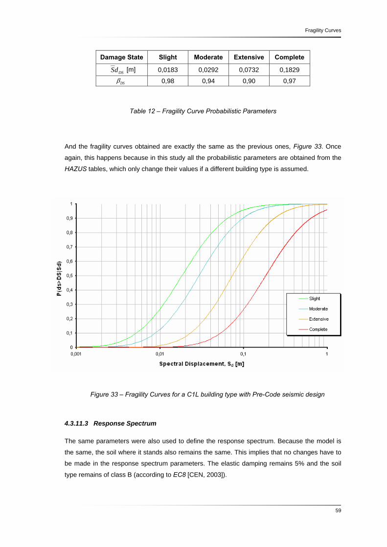
Fragility Curves
59
Damage State Slight Moderate Extensive Complete
DSSd [m] 0,0183 0,0292 0,0732 0,1829
DSβ 0,98 0,94 0,90 0,97
Table 12 – Fragility Curve Probabilistic Parameters
And the fragility curves obtained are exactly the same as the previous ones, Figure 33. Once
again, this happens because in this study all the probabilistic parameters are obtained from the
HAZUS tables, which only change their values if a different building type is assumed.
Figure 33 – Fragility Curves for a C1L building type with Pre-Code seismic design
4.3.11.3 Response Spectrum
The same parameters were also used to define the response spectrum. Because the model is
the same, the soil where it stands also remains the same. This implies that no changes have to
be made in the response spectrum parameters. The elastic damping remains 5% and the soil
type remains of class B (according to EC8 [CEN, 2003]).

Seismic Vulnerability Assessment of Structures using Operational Modal Analysis
60
Eurocode Parameters for Spectral Response, 5%ξ = , Class B soil
S 0β k1 k2 BT CT DT ga η
1,35 2,5 1 2 0,1 0,25 2 1,7 1
Table 13 – Elastic spectral response parameters according to Eurocode 8
For these reasons the response spectrum is the same as presented before in Figure 24 and in
Figure 25 (in spectral coordinates).
4.3.11.4 Solicitation Spectrum
Once again, the bilinear representation of the capacity curve was calculated. The solicitation
spectrum, as it was seen before, is calculated using the effective damping, where the elastic
damping is assumed as 5% for the elastic range. This estimation is presented in Figure 34.
Figure 34 – Bilinear representation of the capacity curve Once the capacity curve configuration changes, the intersection point in the bilinear
representation also changes. This leads to slightly different values for the effective damping.
See Table 14.

Fragility Curves
61
Duration Short Moderate Long
ξE 5
ξH 40,781
K 0,4 0,2 0
ξeff 21,31 13,16 5,00
Table 14 – Effective damping for different soil excitation durations
However, the damping obtained is not enough to change the values of the reduction
coefficients, presented in Table 13. This happens due to the imposition of 0,7η ≥ .
Duration Short Moderate Long η 0,7 0,7 1
Table 15 – Reduction factors for the elastic response spectrum for different soil excitation
durations
As a result, the same response and solicitation spectrums from the first calculations are used.
See Figure 28.
4.3.11.5 Structural Response Estimation
The new capacity curve intersected with the same solicitation spectrum is presented in Figure
35.

Seismic Vulnerability Assessment of Structures using Operational Modal Analysis
62
0
1
2
3
4
5
6
7
0 0,01 0,02 0,03 0,04 0,05 0,06 0,07 0,08Sd [m]
S a [m
/s 2 ]
1
Response Spectrum
Solicitation Spectrum (Short & Moderate)
Capacity Curve
Figure 35 – C1L model type response estimation for Pre-Code design within short and
moderate seismic action duration
Hence, the new spectral displacement response does not change, as it can be seen in Table
16.
C1L Peak Response
Sdr [m] 0,024
Sar [m/s2] 1,114
Table 16 – Spectral peak responses coordinates of the C1L model type for short and moderate
duration of seismic action
With the same purpose as before, the values of cumulative probability are presented on the
next page, in Figure 36.

Fragility Curves
63
Figure 36 – Fragility curves with Spectral Displacement Response for C1L building type and
Pre-Code design level
Moreover, the same probabilities are presented in the discrete form as in Figure 37.
None39%
Slight19%
Moderate31%
Extensive9%
Complete2%
0%
10%
20%
30%
40%
50%
60%
70%
Damage States
Prob
abili
ty o
f Dam
age
.
P(ds
=DS|
Sd)
Figure 37 – Discrete probabilities of structural damage states for the C1L model with Pre-Code design level
With these similar results, the “none” and “moderate” damage states assume once again the
major relevance for this case study. The complete damage probability remains with 2%, the

Seismic Vulnerability Assessment of Structures using Operational Modal Analysis
64
extensive damage state with 9%, the moderate with 31% and the slight and none damage
states with 19% and 39% respectively.
4.3.11.6 Sub-Conclusion
From the previous results one can conclude that the difference between the period taken from
the HAZUS guidelines ( 0, 40 T Hz= ) and the period estimated manually ( 0, 29 T Hz= ) is quite
insignificant when regarding the final probability values achieved.
One possible reason for this to happen may be related with the influence of the period adopted,
the effective modal mass and modal height of the structure.
On one side, the configuration of the capacity curve on the ultimate stage, specifically the
spectral acceleration values, is influenced by the effective modal mass of the building.
On the other side, the values of the yielding capacity range of the curve are determined mainly
by the natural period of the structure.
As it can be seen from the previous plots, the intersection of the capacity curve and the
response spectrum happens in the ultimate range of the building’s resistant capacity. This fact
makes the period value irrelevant for purposes of damage estimation in this specific model
case. As a consequence, only changes on the effective modal mass would result in different
values of damage estimation (with different values of spectral acceleration) or assuming higher
period values in order to try to intersect the capacity curve with the response spectrum still in
the elastic range of the structure.
For this reason, seems logical to try a higher effective modal mass value as well as a higher
period value in order to verify if the intersection is possible still in the yielding capacity of the
model. The inclination of the capacity curve will be higher in the yielding domain. To
demonstrate this fact, the next step will consist on trying a higher period value (e.g. 0,8 T s= ).
Also the possibility of changing the configuration of the fragility curves could have been an
alternative and different probabilities of damage could be achieved for this second step.
Though, for this to happen, one should assume a different value for the effective modal height
(α2) of the building rather than adopting the assumed values provided by HAZUS guidelines.
Even noticing this detail, it would be exaggerated to change this property once with this change
one would assume a different distribution of masses along the height of the building. For this
particular structure (one storey only) this change would not be completely acceptable.

Fragility Curves
65
4.3.12 Procedure according to HAZUS using a different period value:
4.3.12.1 Capacity Curve
In this third and last approach, the period of the structure was assumed with a higher value,
presented in Table 17. To justify this change the author assumes that this particular situation
corresponds, in a practical view of the problem, to the case where the structure has already
suffered some levels of vibration. Due to this fact, its stiffness has been modified. This alteration
on the model’s stiffness can be related e.g. to loss of masonry walls (and with this also changes
in the modal mass can be assumed).
Building Type Cs [-] Te (s) α1 [-] α2 [-] ɣ [-] λ [-] μ [-]
C1L 0,033 0,80 1,05* 1,00 1,50 2,25 5,00
Table 17 – Code building capacity parameters: Design Strength (Cs), Period (Te), Push-Over
Mode Response Factors (α1, α2), Overstrength Ratios (ɣ, λ) and Ductility Factor (μ)
for the C1L building type and for Pre-Code Seismic Design
* The value of α1 has been modified to a value 5% higher in order to check if this parameter has
significant importance on the final results. Note that this parameter can also be determined from
the measurements that can be made using OMA in real structures, which makes it worthy to try
different values.
Therefore, the values obtained for the present case are shown in the next table.
D [m] A [m/s2]
Yielding Capacity 0,008 0,471
Ultimate Capacity 0,084 1,061
Table 18 – Spectral displacements and spectral accelerations for the yielding and ultimate
capacity points

Seismic Vulnerability Assessment of Structures using Operational Modal Analysis
66
And the new correspondent capacity curve plot is represented in the next figure:
Capacity Curve
0
0,2
0,4
0,6
0,8
1
1,2
0 0,02 0,04 0,06 0,08 0,1 0,12
Spectral Displacement [m]
Spec
tral
Acc
eler
atio
n [m
/s
2 ]
Figure 38 – Capacity Curve for C1L building type under the Pre-Code seismic design level
At this point seems relevant to say that the model’s capacity curve has slightly decreased the
peak value of acceleration while the values of spectral displacements have significantly
increased. With this prevision, one can already state that the stiffness of the model has been
reasonably decreased as expected when assuming a higher period value.
4.3.12.2 Fragility Curves
For this third case, the fragility curves will be somewhat different. Once the value of 1α has
changed, the mean spectral displacement has to be adjusted as well. For this reason the
following expression was used:
2DS DSSd r Hδ α= × × (31)
where DSSd is the mean spectral displacement [m]
DSrδ is the inter-storey relative displacement coefficient for the damage state
DS [-]

Fragility Curves
67
2α is the fraction of building effective height [-]
H is the total height of the structure [m]
According to this assumption, the following values were adopted, Table 19.
Damage State Slight Moderate Extensive Complete
DSSd [m] 0,0240 0,0360 0,0960 0,2400
DSβ 0,98 0,94 0,90 0,97
Table 19 – Fragility Curve Probabilistic Parameters for a C1L building type
Consequently, the updated fragility curves are presented in Figure 40.
Figure 39 – Fragility Curves for a C1L building type with Pre-Code seismic design
As it can be seen from the plot of the fragility curves, the cumulative probabilities have slightly
decreased for all the damage states.

Seismic Vulnerability Assessment of Structures using Operational Modal Analysis
68
4.3.12.3 Response Spectrum
For this last case, the response spectrum is still the same. As this happens, the plot remains
intact (see Figures 24 and 25). As it was referred before the response spectrum is a function of
the structure’s damping rate of 5% and of the type of soil where it is situated (according to
Eurocode 8 [CEN, 2003]).
Eurocode Parameters for Spectral Response, 5%ξ = , Class B soil
S 0β k1 k2 BT CT DT ga η
1,35 2,5 1 2 0,1 0,25 2 1,7 1
Table 20 – Elastic spectral response parameters according to Eurocode 8
For this reason only the spectral coordinates normalised spectrum is shown this time.
0
1
2
3
4
5
6
7
0 0,01 0,02 0,03 0,04 0,05 0,06 0,07 0,08
Sd [m]
S a [m
/s 2
]
1
Figure 40 – Normalised Response Spectrum in Spectral Displacement-Spectral Acceleration,
5% damping, Soil Class B

Fragility Curves
69
4.3.12.4 Solicitation Spectrum
In order to obtain the solicitation spectrum, the same assumptions can not be done. For this
purpose it is necessary to once more estimate the bi-linear representation of the new capacity
curve.
As this happens, the bi-linear representation is presented in Figure 41.
Figure 41 - Bilinear representation of the capacity curve
And the effective damping results on the following values, Table 19.
Duration Short Moderate Long
ξE 5
ξH 43,266
K 0,4 0,2 0
ξeff 22,31 13,65 5,00
Table 21 – Effective damping for different soil excitation durations
Note that the value of the hysteretic damping slightly increased, which means that the structure
has increased the effective damping (for short and moderate term actions). These values are in
accordance with the fact that a structure with higher period is more capable to withstand
horizontal dynamic displacements, i.e. able to dissipate more energy. Though, these values are

Seismic Vulnerability Assessment of Structures using Operational Modal Analysis
70
not yet reasonable enough due to the very small difference between when compared to the first
results.
Furthermore, the reduction coefficients based on the effective damping are presented in Table
22.
Duration Short Moderate Long η 0,7 0,7 1
Table 22 – Reduction factor for the elastic response spectrum for different soil excitation
durations
As one can notice, although the effective damping has changed, the reduction factor remains
with the same values as before. Once again, this is due to the imposition of 0,7η ≥ .
Hence, the resultant solicitation spectrums are presented in Figure 31.
0
1
2
3
4
5
6
7
0 0,01 0,02 0,03 0,04 0,05 0,06 0,07 0,08
Sd [m]
Sa [m
/s 2 ]
1
Response Spectrum
Solicitation Spectrum (Short & Moderate)
Solicitation Spectrum (Long)
Figure 42 – Response and solicitation spectrums (according to EC8)
4.3.12.5 Structural Response Estimation
Once again, the structural response estimation results from the intersection of the capacity
curve with the solicitation spectrum previously defined.

Fragility Curves
71
The response estimation for this case is presented in Figure 43.
0
1
2
3
4
5
6
7
0 0,01 0,02 0,03 0,04 0,05 0,06 0,07 0,08
Sd [m]
S a [m
/s 2 ]
1
Response Spectrum
Solicitation Spectrum (Short & Moderate)
Capacity Curve
Figure 43 – C1L model type response estimation for Pre-Code design within short and
moderate seismic action duration
And from this intersection one is able to estimate the value for the spectral displacement,
presented in Table 23.
C1L Peak Response
Sdr [m] 0,028
Sar [m/s2] 0,913 Table 23 – Spectral peak responses coordinates of the C1L model type for short and moderate
duration of seismic action
Notice that the spectral displacement peak response has increased to a value of 0,028 m. This
is in accordance with the decrease of stiffness of the model. On the other hand, also the value
of spectral acceleration has suffered a decrease. The intersection is now happening on the
yielding range of the structure.
Finally, the spectral displacement in the fragility curves plot will give the possibility to estimate
the cumulative probabilities for the structural model damage states.

Seismic Vulnerability Assessment of Structures using Operational Modal Analysis
72
Figure 44 – Fragility curves with Spectral Displacement Response for C1L building type and
Pre-Code design level
Finally, the same probabilities in the discrete form are presented.
None46%
Slight16%
Moderate30%
Extensive7% Complete
1%0%
10%
20%
30%
40%
50%
60%
70%
Damage States
Prob
abili
ty o
f Dam
age
.
P(ds
=DS|
Sd)
Figure 45 - Discrete probabilities of structural damage states for the C1L model with Pre-Code
design

Fragility Curves
73
4.3.12.6 Sub-Conclusion
According to the new probability values, the vulnerability of the structure changed for a lower
standard. For higher periods and higher effective modal mass, the percentage related to the
highest damage levels decreases significantly while it is clear the increase of the probability
values for the safest damage states. It is obvious that the problematic damage states have
decreased their probability of happening in the structure in order to raise the values of the
damage state connoted with no damage at all. From the plot, it is possible to assume that the
complete damage state decreased from 2% to 1%. The values of the extensive and moderate
damages slightly decreased from 9% to 7% and from 31% to 30%, respectively. The slight
damage state decreased from 19% to 16%, while the level that is associated with no damage
on the structure has increased 7%.
In general, the vulnerability of the structure has decreased. These conclusions are in
accordance with the expected values and the intersection of the capacity curve with the
response spectrum is now undoubtedly located on the yielding range of the capacity curve and
the influence of the period and effective modal mass on the damage vulnerability assessment of
the model are clearly verified.
4.4 ERROR PREDICTION AND EVALUATION INTRODUCING OMA INFORMATION
4.4.1 Fragility Curves out of HAZUS Guidelines
The performance of a structure evaluated under the HAZUS-MH MR1 Guidelines [FEMA, 2003]
constitutes a reasonable and efficient method to estimate seismic vulnerability. Though, it is
comprehensive that this method has its limited range. In general, the total variability of each
case is dependent of some particular aspects as the uncertainty of the damage state threshold,
the variability in the capacity response of the structural system and the uncertainty related with
the spatial variability of ground motion demand. As this happens, the values obtained from this
procedure are assumed to have a range of possible factors that could have strong influence on
the final results. It is aware to express that evaluations which result from this method surely
represent median estimates of the structure’s capacity and behaviour.
For capacity estimations the variability of each building type is assumed to vary up to 25% for
code-designed buildings (i.e. High-code, Moderate-code and Low-code seismic design levels)
and 30% for Pre-code buildings [FEMA, 2003].

Seismic Vulnerability Assessment of Structures using Operational Modal Analysis
74
When it comes to the construction of fragility curves, also the same uncertainty is expected.
These curves are defined, as said on previous chapters, by lognormal functions where the
mean and standard deviation values are taken into account.
On the other hand, the demand spectrums are influenced by the earthquake source (e.g.
estimations and functions used by the National or European Codes), by earthquake magnitude,
distance from the source to the site, soil conditions (e.g. whether if it’s rocky or sandy soil) and
also by the effective damping which varies according to the building’s properties and earthquake
duration (e.g. Short, Moderate or Long duration).
4.4.2 Fragility Curves out of Operational Modal Analysis
When performing Operational Modal Analysis, errors that are inherently related to the
measurements are very small. For this reason, it seems very appropriate to think about OMA as
an incredibly useful tool to estimate modal characteristics of structural systems. Once one has
the estimated period, effective modal height and effective modal mass the methodology of
vulnerability assessment by means of fragility curves achieves an higher standard where
accuracy will be supposedly improved.
At this point, once the method without the help of Operational Modal Analysis has been
performed, seems more than time to try to fit the capacities of OMA within the extents of a
nonlinear static analysis. The question that rises at this point is: How could we introduce OMA
into the field of seismic engineering?
From a simple point of view, it is reasonable to admit that OMA would bring an easy method to
estimate modal characteristics of any kind of structure. Let’s suppose one is trying to estimate
the level of damage in the reduced model after the action of an earthquake.
On the first hand we have the measurements taken before the earthquake. This data provides
the engineer with the initial modal characteristics such as the fundamental period, the
configuration of the mode shapes and even the damping ratios (e.g. if using the Stochastic
Subspace Identification technique). As it was shown before in the HAZUS methodology, the
elastic period and the effective modal mass are really important parameters which allow the
characterization of the fragility curves and, in addition, the estimation of the probability of
damage of the model.
The idea is to perform exactly the same evaluation after the induced damage is done. It is
known that after the main shock, the modal characteristics of the structure significantly change if
the damage is substantial. The use of OMA to perform the same measurements will provide the

Fragility Curves
75
user with the new exact values of period, mode shapes and damping. These parameters, now
with different values, will allow the estimation of the susceptibility of the structure to damage.
Comparisons can be made regarding the stiffness of the system and future precautions can be
carried out.
In this project, the measurements in a real structure were not possible to perform. For this
reason, the idea is presented here under an hypothetic assumption that everything can be done
in the future. Nevertheless, the possibility of using OMA in future damage assessments and the
confirmation that nonlinear static analysis can be improved with this technique was here
indubitably recognized.
4.4.2.1 Error Estimation in Modal Identification
Additionally, when treating the identification of the mode shapes, in the worst scenarios the
author risks to say that the maximum error will be situated around 1%. This is not true when the
user prefers to apply pre-standard proceedings, estimated calculations or even the most
complex finite element model rather than modal identification techniques.
For the present case of study, the number of frequency lines is 1024, the sampling frequency is
150 Hz (already decimated) and the fundamental frequency has the value of 10,84 Hz. With
these values one can estimate the percentage of error incorporated in this particular
Operational Modal Analysis measurement.
. 2 1024 13,62 2 75
freq lines
Nyquist
nT s
f×
= = =× ×
(32)
1
1
1 1 0,073513,6
10,84
0,074 0,0068 0,68%10,84
(Fundamental Mode)
f HzT
f Hz
ff
Δ = = =
=
Δ= =
As it is possible to see, the results provided with real data are extremely accurate when it comes
to modal identification. It is important to refer that this error estimation is only related with the
modal identification and it can not be assumed for the whole process of damage estimation.

Seismic Vulnerability Assessment of Structures using Operational Modal Analysis
76

Summary and Conclusions
77
5 Summary and Conclusions
5.1 SUMMARY
In the present work a quantitative study of the seismic vulnerability assessment was
undertaken. The intention to verify the level of influence that the elastic period has in order to
estimate damage in structures under the assumptions precompiled by HAZUS was always the
main purpose. Some different values for this parameter were assumed and some results were
questioned. The applicability of OMA (by using it for estimation of modal parameters) in the
seismic domain was faced has a possibility to improve existent methods or develop new ones.
In the beginning, the possibility to integrate Operational Modal Analysis as a powerful and
helpful tool to successfully estimate modal parameters of a certain structure intended to be a
parallel purpose of this investigation. It was believed that OMA would introduce to the results an
accuracy that would greatly improve the reliability of damage probabilities estimated under
HAZUS Guidelines, especially concerning to frequencies and mode shapes associated to the
first modes of the structure. The method applied in this thesis was based under certain rules
proposed by the Federal Emergency Management Agency under the HAZUS-MH MR1
Technical Manual [FEMA, 2003] and OMA was not used for this purpose. Additionally, fragility
curves were built and certain assumptions had to be made.
Later on, while performing the intrinsic calculations of the method adopted from HAZUS, the
results achieved helped to conclude some facts. The difference in the period of the model
showed no significant influence for the final results if the structures response is already in the
ultimate range of capacity. If this happens, the intersection point with the response spectrum will
always be the same, no matter what period the model has. A possible cause for this to happen
may reside in the facts that either the structure adopted and the assumptions done were not the
best or the method itself turned out to be predominantly conservative for this particular simple
structure.
The results achieved, while not precluding the successful application of Operational Modal
Analysis to a far-reaching extent in this domain, do demonstrate that the method considered,
where a multi degree of freedom system is substituted by an equivalent single degree of

Seismic Vulnerability Assessment of Structures using Operational Modal Analysis
78
freedom system, is much more sensitive to changes in modal mass and height rather than in
period deviations.
From the work performed in this dissertation, although it was not possible to test a real building
with real measurements as initially desired, the reduced models studied clearly show that it may
be possible to do it with quite satisfactory results. In fact, this thesis can be seen as a primary
glimpse for future investigations in this field and its content is purely hypothetical for now.
Nevertheless, one can conclude that the two domains of engineering can reasonably achieve
promising estimations when working together.
5.2 CONCLUSIONS
Concerning the European regulamentation, the possibility to proceed with nonlinear static
analysis seems finally accepted. This kind of analysis turns out to be one of the most trustable
methods that engineers have on their disposal in the present days to estimate the behaviour of
a structural system subjected to strong ground motion. Even though with some complexity
attached, these methods revealed their practical side due to the approximate way of
reproducing the inelastic behaviour of several structural components. The virtuous advantages
when compared to linear methods, usually applied in daily projects, are significantly high.
Nevertheless, it is also necessary to recognise that the carefulness when relying on these
methods has to be refined to higher standards. It is necessary to have extra caution in the
method chosen, in the assumptions adopted for the modulation and the several phenomena
related to the problem have to be well known. A lack of clear and complete conceptual
understanding of constructed system behaviours, events and phenomena affecting these
behaviours is unavoidable. A reasonable and critical perspective should not be dismissed and
the errors that are intrinsically connected with these methods should constantly be kept in mind.
When it comes to the specific results obtained in this project, one can conclude that the
“HAZUS-MH MR1 Technical Manual” [FEMA, 2003] surely provides a reasonable and expedite
method to estimate damage in structures. At the same time, the use of push-over analysis and
fragility curves denote a quite conservative approach regarding real and practical data,
specifically when dealing with a particular range of elastic periods. Additionally, these guidelines
always refer to typical American building types, which propelled the author to perform some
adaptations in order to achieve reasonable results for the proposed model. For example, the
response spectrums which allow characterizing the seismic action were calibrated to reflect the
Portuguese seismic casualty (Type 1 seismic zone for Lisbon; Type 1 seismic action). The
capacity curve of the structure was totally estimated under the HAZUS assumptions and the
fragility curves used to characterize the exceeding probabilities for the several damage states

Summary and Conclusions
79
were stipulated by the same method. Though, once the solicitation spectrum is unchangeable
(i.e. the same reduction coefficient was achieved for different values of effective damping), the
fragility and capacity curves turned out to be decisive during the process. When it comes to the
fragility curves, one knows that the parameter that could have changed their configuration could
be the mean spectral displacement. This parameter, according to HAZUS proceedings, is
dependent on the modal height (as it can be seen in Point 4.3.12.2). Meanwhile, the capacity
curve is dependent on the modal mass of the structure (Point 4.3.10.1). Nevertheless, the main
purpose was to understand how the results would be different if different values of period were
adopted and such changes were not part of the expected results. Though, it is important to refer
that both parameters can be accurately estimated with OMA procedures.
Such integrated inspection and calculations through HAZUS assumptions have revealed that
damage states such as “None” and “Moderate” assume quite a big importance for this specific
model case.
On the other side, Operational Modal Analysis proved to be particularly exact. This fact was
confirmed from the illustrative study of the laboratory model, where ambient vibration tests were
performed in order to estimate the real elastic period and mode shapes of the structure. The
accuracy of Operational Modal Analysis was certainly confirmed with the illustrative example.
Regarding the results achieved, one can refer that the purpose of this thesis was somehow
accomplished. Now it is possible to say that the influence of the period when performing this
method is quite important. Though, if the correspondent quantification of the modal masses and
heights are not efficiently estimated the expected results can be ambiguous. Consequently, it is
unavoidable to refer that for this specific case, where several assumptions were carried out,
Operational Modal Analysis appears not to be substantially decisive once the model adopted
was too simple. At this point it seems important to say that for a real structure, the same
situation would not be expected. Operational Modal Analysis when performed in a real structure
certainly will improve the final results because fewer assumptions will be considered and
certainly the real building will be higher (with multiple storeys) which will allow its reduction to a
simple degree of freedom system.
It is comprehensive that for some investigators, this work can look incomplete due to the lack of
information about how OMA really actuates if we use it in real structures for damage
assessment. Nevertheless, the correlation between theoretical and experimental modal
parameters, seem to provide sufficient verification of the models main assumptions and the
proposed method clearly promises future successful applicability.

Seismic Vulnerability Assessment of Structures using Operational Modal Analysis
80
5.3 RECOMMENDATIONS FOR FUTURE RESEARCHES
In this present work only push-over analysis was performed in a very simple model of one
storey. For future investigations on this area it is suggested the utilization of different methods to
estimate post-earthquake damage on structures and the utilization of a higher model (if possible
a real building) in order to obtain more satisfactory changes in modal characteristics. For
example, a recent technique that probably will provide the engineer with new advantages is
designated as Incremental Analysis.
Alternatively, it is also proposed the adaptation of this present methodology provided by HAZUS
to the European case, i.e. to the quantification of damage in European typologies that would
render the European type of construction and the correspondent calibration of all the
parameters that are integrated in this type of analysis.
Concerning to modal identification of structures, some other techniques and algorithms can be
used. When analysing real structures, not always the FDD is a possible solution. The extent to
future investigations with Enhanced Frequency Domain Decomposition (where damping rates
can be estimated, which are essential to define the reduction coefficient of the solicitation
spectrum) can also be an exciting challenge.

References
81
REFERENCES
[Aenlle et. al., 2003] Aenlle, M., Brincker, R. and Cantelli, F. “Load Estimation from Natural
Input Modal Analysis”, Proceedings of XXIII International Modal Analysis Conference, Texas,
USA, 2003.
[Andersen et. al., 2000] Andersen P., Brincker, R. and Zhang, L. “Modal Identification from
Ambient Responses using Frequency Domain Decomposition”, 18th International Modal
Analysis Conference, San Antonio, Texas, USA, 2000.
[Bendat et. al., 1993] Bendat, J. S. and Piersol, A. G. “Engineering Applications of
Correlation and Spectral Analysis”, John Wiley & Sons, 1993.
[Brincker et. al., 2000] Brincker, R., Ventura, C. and Andersen P. “Why Output-Only Modal
Testing is a Desirable Tool for a Wide Range of Practical Applications”, Proceedings of IMAC
XXI, Texas, USA, 2003.
[Campos Costa, 2007] Campos Costa, A., Sousa, M. L., Carvalho, A., Cansado Carvalho, E.,
“Definição da Acção Sísmica em Portugal Continental para a Preparação do Anexo Nacional,
Parte 1, Eurocódigo 8”, 7º Encontro Nacional de Sismologia e Engenharia Sísmica, FEUP,
Porto, 2007.
[Candeias, 2000] Candeias, P. “Avaliação Sísmica de Edifícios Existentes – Contribuição
para a Avaliação da Vulnerabilidade em Portugal”, Master Thesis, IST, 2000.
[CEN, 1998] “European Pre-Code ENV-1998-1-1:1994: Eurocode 8 – Design
provisions for earthquake resistance of structures”, CEN, 1998.
[Cunha, 2005] Cunha, A. and Caetano, E. “From Input-Output to Output-Only Modal
Identification of Civil Engineering Structures”, IOMAC, Denmark, 2005.

Seismic Vulnerability Assessment of Structures using Operational Modal Analysis
82
[FEMA, 2003] “HAZUS-MH MR1 - Technical Manual”, Federal Emergency
Management Agency, Washington D.C., USA, 2003.
[Ferreira, 2000] Ferreira, P. “Output-Only Modal Testing and Identification – Seismic
Vulnerability Assessment of the Building Nº4 of the Hospital de Santa Maria”, Master Thesis,
IST, 2000.
[Hansen, Pedersen, 2007] Hansen, S., Pedersen, I. “Load Estimation by Frequency
Domain Decomposition”, 9th Semester Project, Aalborg University, 2007
[Nielsen, 2000] Nielsen, S. “Vibration Theory Volume 3 – Linear Stochastic Vibration
Theory”, 3rd Edition, Aalborg Tekniske Universitetsforlag, 2000.
[SAP2000 v10] “SAP2000 Advanced version 10.0.7 - Structural Analysis Program”,
Computers and Structures, Inc., Berkeley, California, USA, 1976-2006.
[SVIBS] ARTeMIS Extractor: Ambient Response Testing and Modal
Identification Software, Structural Vibration Solutions, Inc., ©1993-2004 Structural Vibration
Solutions, Inc.
[Zill et. al., 2001] Zill, D., Cullen, M. “Differential Equation with Boundary-Value
Problems”, 5th Edition, Brooks and Cole, 2001.

Appendix A
83
Appendix A:
Seismic Waves
Several series of waves emanate from the focus of an earthquake. They have different speeds
and produce different effects as they travel through the lithosphere. In this appendix a brief
explanation of their different forms is introduced.
The seismic waves move through the bodies by means of ondulatory movements. Considering
their different characteristics, the waves can be separated in two main types, which are here
described.
Body Waves
These kinds of waves travel through the interior of the Earth and their interaction with the planet
is one of the best indicators about the core composition. They present deformed radial traces
(where the origin is the hypocentre) due to the variation of density and composition of the
interior of the Earth. This effect can be compared to the refraction of the light through some
bodies.
The body waves are responsible for the first shakings during a seismic event as well as for the
major vibration felt after it. There are two kinds of body waves:
Primary Waves (P) - these waves are the fastest of all. They are characterized for producing
longitudinal deformations which make the rocks vibrate in parallel with the direction of
propagation of the wave. It is verified an alternate compression and distension with low periods

Seismic Vulnerability Assessment of Structures using Operational Modal Analysis
84
and amplitudes while the wave travels through the material, producing elastic alterations of
volume on the rock.
Figure 46 – Primary wave movement
If these “pression waves” would travel through the air, they would be sound waves, travelling at
the speed of sound. Though, its velocity depends on the material it crosses: about 330 m/s in
the air, 1450 m/s in water and 5000 m/s in granite. The velocity of this kind of wave can be
calculated using the following formula:
( 4 / 3)P
Kv μρ
⎛ ⎞+= ⎜ ⎟
⎝ ⎠ [m/s]
where, K is the modulus of incompressibility
μ is the modulus of rigidity of the material (for liquids, μ =0)
ρ is the density of the material through which the wave is propagating

Appendix A
85
Secondary Waves (S) – The secondary waves (or shear waves) are transversal waves where
the medium is displaced perpendicularly to the direction of propagation of the wave. In this case
the rocks are shacked horizontally from one side to another alternately.
Figure 47 – Secondary wave movement
These ones are slower than the P waves (around 60% of the P waves speed), with velocities
between 2000 and 5000 m/s, usually being the second fastest type of wave (that’s the reason
why they are designated secondary).
Sv μρ
⎛ ⎞= ⎜ ⎟
⎝ ⎠ [m/s]
where, μ is the shear modulus / rigidity modulus of the medium
ρ is the density of the material through which the wave is propagating

Seismic Vulnerability Assessment of Structures using Operational Modal Analysis
86
The wave moves through elastic mediums, and the main restoring force comes from shear
effects. Hence, as they flow with shear forces they can’t pass through liquids. These waves are
divergenceless and obey the continuity equation for incompressible media.
Surface Waves
When the earthquake focus is not too deep, i.e. when it happens in the upper layers of the
lithosphere, it creates surface waves that start in the epicentre and have a more complex and
destructive deforming force. They are similar to water waves when a rock drops into its surface.
Although these waves are slower than the body waves they are usually much more destructive
due to the low frequencies, long durations and big amplitudes. Two types are distinguished:
Rayleigh waves and Love waves.
Rayleigh Waves (R) – these types of waves are the result of the interaction between P and S
waves at the surface of the Earth. As it passes, a surface particle moves in a circle or ellipse in
the direction of propagation. Harmonics of the Rayleigh wave move particles in regions that
alternate elliptical motion with nodes of no-movement.
Figure 48 – Rayleigh wave movement

Appendix A
87
The maximum distance that Rayleigh waves move particles (amplitude) decreases rapidly with
depth in the material. Rayleigh waves travel along the surface of the earth at about 10 times the
speed of sound in air.
Love Waves (L) – Usually the most destructive waves of all and what most people feel directly
during an earthquake. They travel through the soil by means of horizontal shifting of the soil that
causes an elastic movement of the rocks on an horizontal plane perpendicular to the wave
direction, just like a snake along the ground. Note that the amplitude or maximum particle
horizontal displacement decreases rapidly as one examines deeper layers in depth. Their name
comes related with the scientist who predicted their existence mathematically around 1911,
A.E.H. Love.
Figure 49 – Love wave movement

Seismic Vulnerability Assessment of Structures using Operational Modal Analysis
88

Appendix B
89
Appendix B:
Earthquake Magnitude
Seismic magnitude consists on a quantitative evaluation of the energy released by the
hypocentre of an earthquake and is measured on a decimal logarithmic scale, developed by C.
Richter. He showed that, the larger the intensity of an earthquake, the larger the amplitude of
ground motion at a given distance. He calibrated his scale of magnitudes using measured
maximum amplitudes of shear waves on seismometers particularly sensitive with periods of
about one second. The fundamental expression to obtain the level of magnitude is given by:
10logM A C= −
where, A is the maximum amplitude recorded in a seismograph (in mm)
C is the distance correlation factor (obtained from tables found in his own
book called “Elementary Seismology”)
Magnitude is independent of the location of the seismograph, owing to adequate correction of
distances between its location and the source. Even though the magnitude provides the
engineer a quantitative measure of the event, recorded diagrams of accelerations, velocities
and displacements provide the basis for practical design, especially the amplitude, frequency
and duration of the event.
The Richter scale, frequently used in present days to estimate magnitudes of earthquakes is
presented on the next table.
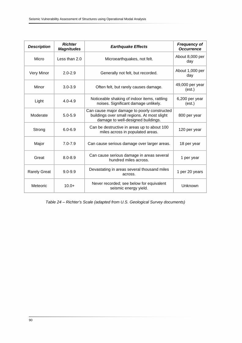
Seismic Vulnerability Assessment of Structures using Operational Modal Analysis
90
Description Richter Magnitudes Earthquake Effects Frequency of
Occurrence
Micro Less than 2.0 Microearthquakes, not felt. About 8,000 per day
Very Minor 2.0-2.9 Generally not felt, but recorded. About 1,000 per day
Minor 3.0-3.9 Often felt, but rarely causes damage. 49,000 per year (est.)
Light 4.0-4.9 Noticeable shaking of indoor items, rattling noises. Significant damage unlikely.
6,200 per year (est.)
Moderate 5.0-5.9 Can cause major damage to poorly constructed
buildings over small regions. At most slight damage to well-designed buildings.
800 per year
Strong 6.0-6.9 Can be destructive in areas up to about 100 miles across in populated areas. 120 per year
Major 7.0-7.9 Can cause serious damage over larger areas. 18 per year
Great 8.0-8.9 Can cause serious damage in areas several hundred miles across. 1 per year
Rarely Great 9.0-9.9 Devastating in areas several thousand miles across. 1 per 20 years
Meteoric 10.0+ Never recorded; see below for equivalent seismic energy yield. Unknown
Table 24 – Richter’s Scale (adapted from U.S. Geological Survey documents)

Appendix C
91
Appendix C:
Earthquake Intensity
Seismic intensity is a way of qualitative measuring that describes the effects produced by
earthquakes in the surface of the earth. The evaluation of seismic intensity is done by means of
observation of damage in structures and people. A known scale is the “Modified Mercalli” (MM)
scale, given in Roman numerals (from I to XII), which is actually the best way to classify the
intensity of an earthquake. Note that the Mercalli scale is purely qualitative, is based only in
direct observation of real facts and shouldn’t be used in practical design.
For example, if an earthquake with magnitude eight in the Richter scale happens in a deserted
place will correspond to a Level I in the Mercalli scale because there is no damage at all. The
Mercalli scale is briefly described on the next pictures.
I - Not Felt
Not felt except by a very few under
especially favourable conditions.
Figure 50 – Mercalli intensity level I (M1)

Seismic Vulnerability Assessment of Structures using Operational Modal Analysis
92
II - Feeble Felt only by a few persons at rest,
especially on upper floors of
buildings or favourably placed.
Delicately suspended objects may
swing.
Figure 51 – Mercalli intensity level II (M2)
III - Slight
Felt indoors by few people.
Hanging objects swing. Vibration
like passing of light trucks.
Duration estimated. May not be
recognized as an earthquake.
Figure 52 - Mercalli intensity level III (M3)
IV - Moderate
Felt indoors by many, outdoors by
few during the day. At night, some
awakened. Dishes, windows, doors
disturbed; walls make cracking
sound. Sensation like a heavy truck
striking building. Standing motor
cars rocked noticeably. Dishes and
windows rattle alarmingly.
Figure 53 - Mercalli intensity level IV (M4)

Appendix C
93
V – Rather Strong Felt outdoors by nearly everyone.
Direction estimated. Sleepers
awakened. Liquids disturbed. Small
unstable objects displaced. Doors
swing. Shutters, pictures move.
Pendulum clocks change rate.
Figure 54 - Mercalli intensity level V (M5)
VI – Strong Felt by all. Many frightened and run
outdoors. Persons walk unsteadily.
Windows, dishes, glassware
broken. Books off shelves. Pictures
off walls. Furniture moved. Weak
plaster or masonry cracked. Small
bells ring. Trees shaken visibly.
Figure 55 - Mercalli intensity level VI (M6)
VII – Very Strong
Difficult to stand. Noticed by drivers.
Hanging objects quiver. Furniture
broken. Damage and cracks to
masonry, Weak chimneys broken.
Fall of plaster, bricks, stones, tiles
and architectural ornaments. Waves
on ponds. Large bells ring.
Figure 56 - Mercalli intensity level VII (M7)

Seismic Vulnerability Assessment of Structures using Operational Modal Analysis
94
VIII – Destructive Steering of cars affected. Slight
damage in specially designed
structures; considerable buildings
with partial collapse. Great damage
in poorly built structures. Fall of
chimneys, factory stacks, columns,
monuments, walls. Heavy furniture
moved. Branches broken from trees.
Figure 57 - Mercalli intensity level VIII (M8)
IX – Ruinous General panic. Considerable
damage in specially designed
structures, well designed frame
structures thrown out. Great
damage in substantial buildings,
with partial collapse. Buildings
shifted off foundations.
Underground pipes broken.
Figure 58 - Mercalli intensity level IX (M9)
X – Disastrous
Some well built wooden structures
destroyed; most masonry and
frame structures destroyed. Rails
bent Some bridges destroyed.
Serious damage to dams, dikes,
embankments. Large landslides.
Sand and mud shifted horizontally
on beaches. Rails bent slightly.
Figure 59 - Mercalli intensity level X (M10)

Appendix C
95
XI – Very Disastrous
Few, if any masonry structures
remain standing. Bridges
destroyed. Rails bent greatly.
Underground pipelines completely
out of service.
Figure 60 - Mercalli intensity level XI (M11)
XII – Catastrophic Total damage - Almost everything is
destroyed. Lines of sight and level
distorted. Objects thrown into the
air. The ground moves in waves or
ripples. Large amounts of rock may
move.
Figure 61 - Mercalli intensity level XII (M12)

Seismic Vulnerability Assessment of Structures using Operational Modal Analysis
96

Appendix D
97
Appendix D:
Introduction to Linear Waves
According to Newton, who discovered that sunlight can be decomposed in its spectrum of
colours, stating that the principle of the white light consists of numerous components of light of
various colours (different in wave length or wave frequency), also the energy of a wave is
distributed over frequency for the same reasons.
The spectral analysis consists in decomposing a complex physical phenomenon (like waves)
into their individual components with respect to frequency.
For this work one is interested in understanding the spectral analysis of irregular waves which is
the phenomenon related with the vibrations that occur in real structures. Vibrations are nothing
more than waves that propagate through materials.
Thus, the objective of understanding this concept (vibrations in the frequency domain) is directly
engaged with the possibility of avoiding the frequency where the wave energy concentrates in
order to build structures with distant resonance frequencies and with this avoid the amplification
of force and deformation.
Before we can proceed to the Operational Modal Analysis itself, some basic concepts about
linear wave theory are briefly explained.

Seismic Vulnerability Assessment of Structures using Operational Modal Analysis
98
Surface elevation of a linear wave:
The surface elevation of a linear wave in order to position (x) and time (t), is:
( , ) .cos( - ) .cos( - )2
Hx t wt kx a wt kxη δ δ= + = +
where H is the wave height
a is the amplitude, 2Ha =
w is the angular frequency, 2wL
=
T is the wave period
k is the wave number
L is the wave length
δ is the initial phase
This expression can also be simplified if we define the observation point to x=0 and then we
have:
( ) .cos( ) t a wtη δ= + [Joule/m2]
Wave Energy:
The average energy present in a wave per unit area can be determined by:
2 21 1. . . . . .8 2
= = E g H g aρ ρ [Joule/m2]

Appendix D
99
Variance of surface elevation of a linear wave:
The variance of the surface elevation of a sinus wave is (note that in this case E refers to
“Expectation”),
2
2
2
0
2
[ ( )] [( ( ) ( )) ][( ( )) ]
1 ( )
12
=
=
=
T
Var t E t tE t
t dtT
a
η η η
η
η
= −
∫
Superposition of linear waves:
It is known by mathematicians that since the governing equation (Laplace equation) and
boundary conditions are linear in small amplitude wave theory, that they are superposable. This
means that if we combine all the different number of linear waves with different wave heights
and different wave periods the result will be an irregular wave surface elevation.
A simple preview of how it is constructed can be seen in the figure presented on the following
page.

Seismic Vulnerability Assessment of Structures using Operational Modal Analysis
100
Wave 1:
H=H1 ; f=f1 ; a=a1
+
Wave 2:
H=H2 ; f=f2 ; a=a2
+
Wave 3:
H=H3 ; f=f3 ; a=a3
+
Wave 4:
H=H4 ; f=f4 ; a=a4
=
Superposition
Figure 62 – Superposition of periodic waves
Surface elevation of an irregular wave:
The superposed wave surface elevation is obtained from a sum of the component waves and its
value can be obtained from the next equation:
1 1
( ) ( ) .cos( ) i i
i i i ii i
t t a w tη η δ= =
= = +∑ ∑
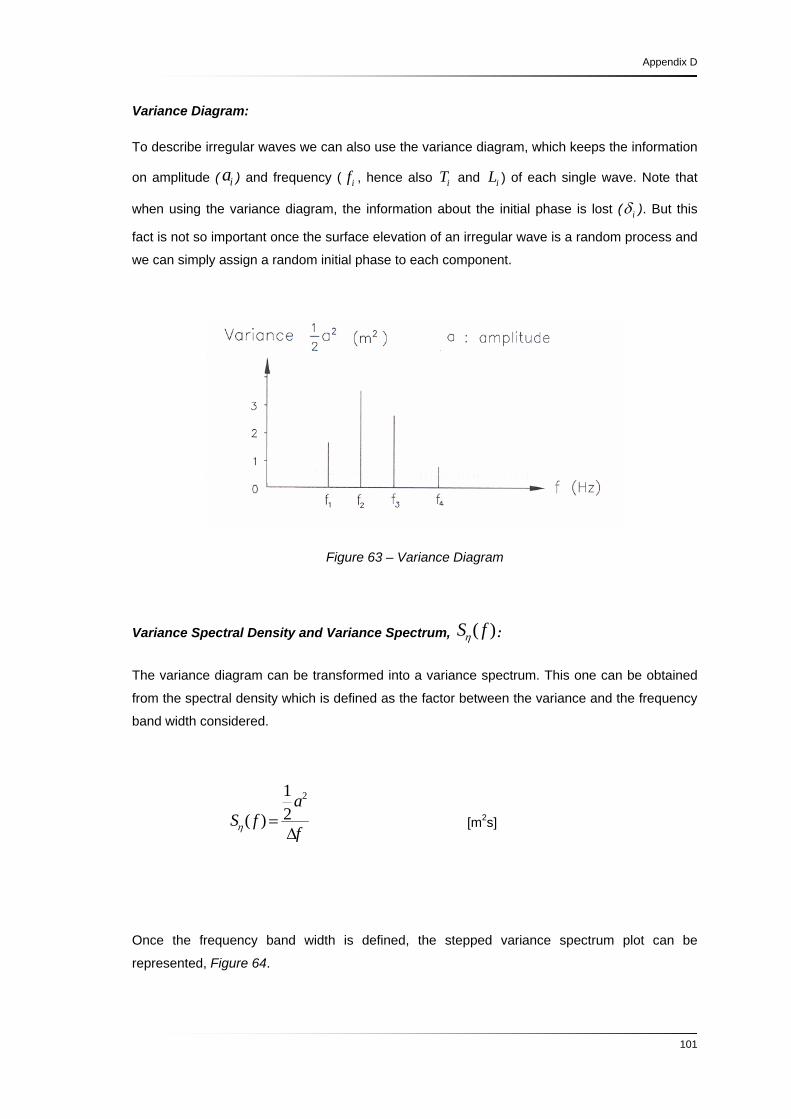
Appendix D
101
Variance Diagram:
To describe irregular waves we can also use the variance diagram, which keeps the information
on amplitude ( ia ) and frequency ( if , hence also iT and iL ) of each single wave. Note that
when using the variance diagram, the information about the initial phase is lost ( iδ ). But this
fact is not so important once the surface elevation of an irregular wave is a random process and
we can simply assign a random initial phase to each component.
Figure 63 – Variance Diagram
Variance Spectral Density and Variance Spectrum, ( )S fη :
The variance diagram can be transformed into a variance spectrum. This one can be obtained
from the spectral density which is defined as the factor between the variance and the frequency
band width considered.
212( )
aS f
fη =Δ
[m2s]
Once the frequency band width is defined, the stepped variance spectrum plot can be
represented, Figure 64.

Seismic Vulnerability Assessment of Structures using Operational Modal Analysis
102
Figure 64 – Stepped Variance Diagram
As it was already said before, an irregular wave is composed of N waves. In the limit, infinite
waves with infinite different frequencies can compose an irregular wave. As this happens, the
value of the frequency band width ( fΔ ) approaches zero because the values of frequency are
so many that they become more and more close to each other. Consequently, the stepped
variance spectrum becomes a continuous variance curve, therefore we can also call it as
energy spectrum.
Figure 65 – Continuous Variance Diagram

Appendix D
103
Hence, the energy spectral density can be defined as:
21. . .2( )
g aES ff fη
ρ= =
Δ Δ [J.s/m2]

Seismic Vulnerability Assessment of Structures using Operational Modal Analysis
104

Appendix E
105
Appendix E:
Singular Value Decomposition, SVD
According to the basic algorithm in linear algebra, the process to invert a 2x2 matrix A is easily
exemplified as follows:
If a b
Ac d⎡ ⎤
= ⎢ ⎥⎣ ⎦
then 1 1 .det( )
d bA
c aA− −⎡ ⎤= ⎢ ⎥−⎣ ⎦
where det( ) . .A a d b c= −
Although this is true for some cases, when the determinant of matrix A is equal to zero, the
matrix is called singular and its inverse cannot be determined by this simple way. Hence, other
algorithms have to be used.
In this project, the use of Singular Value Decomposition is essential to calculate the frequencies
and mode shapes of the structural system in analysis. When using FDD technique the values of
these parameters are dependent on the matrices that result from the SVD algorithm. The SVD
algorithm is used in the frequency domain decomposition in order to estimate the mode shape
vectors corresponding to a peak picked eigenfrequency, i.e. from the singular vectors. [Hansen,
Pedersen, 2007]
In linear algebra, the Singular Value Decomposition (SVD) consists in the factorization of a
rectangular real or complex matrix. The spectral theorem states that normal matrices can be

Seismic Vulnerability Assessment of Structures using Operational Modal Analysis
106
unitarily diagonalized using a basis of eigenvectors. The SVD can be regarded as a
generalization of the spectral theorem to arbitrary, not necessarily square matrices.
Suppose A as an m x n matrix in the field of real or complex numbers. Then, there exists a
factorization of the form:
. . TA U V= Σ
where the superscript T
denotes the transpose of V . For complex matrices the superscript
His preferred, which is the conjugate transpose of the matrix.
The decomposition of a matrix A involves the existence of a diagonal m x n matrix Σ of the
form:
00 0D⎡ ⎤
Σ = ⎢ ⎥⎣ ⎦
where D can be a d x d matrix, also diagonal. The value of d should not be higher than m or n
and represents the rank of matrix A .
To any factorization of the type . . TA U V= Σ , with positive diagonal entries in D , with an
orthogonal m x m matrix called U and an orthogonal n x n matrix called V is called a
Singular Value Decomposition or SVD of A .
The matrices U and V are not uniquely determined by A , but the diagonal entries of Σ are
necessarily the singular values of A . The matrix U contains a set of orthonormal “output”
basis vector directions for A . The matrix V contains a set of orthonormal “input” basis
directions for A . And the matrix Σ , contains the singular values in decreasing order in the
diagonal, which can be thought as scalar numbers by which each corresponding input is
multiplied to obtain a correspondent output. The singular values is are equal to the square root
of the eigenvalues iλ of the problem.

Appendix E
107
Hence, the Σ matrix achieves the following form:
1 10 0 0 00 0 0 0
0 00 0i i
ii
s
s
λ
λ×
⎡ ⎤ ⎡ ⎤⎢ ⎥ ⎢ ⎥Σ = =⎢ ⎥ ⎢ ⎥⎢ ⎥ ⎢ ⎥⎣ ⎦⎣ ⎦
, where 1...is s> >
The SVD can be also applied extensively to the study of other linear inverse problems. It is
widely used in statistics where it is related to principal component analysis, signal processing
and pattern recognition and also in weather prediction studies where rather larger matrices are
used.

Seismic Vulnerability Assessment of Structures using Operational Modal Analysis
108

Appendix F
109
Appendix F:
Eigenfrequencies
When using FDD techniques, the eigenfrequencies can be obtained simply by peak picking the
singular values from the auto spectral density diagram. The energy which is concentrated
around the values of the eigenfrequencies is confirmed through the peaks that rise at these
values vicinity. For an illustrative purpose only the first three frequencies will be presented. On
the plot of spectral densities, Figure 66, it is seen that the peaks rise around the frequencies
1 10, 4 f Hz= , 2 11,3 f Hz= and 3 16,1f Hz= . The eigenfrequencies are situated at the peak
value. Each line represents one channel, i.e. one accelerometer recording.
Figure 66 – Singular Values obtained from the SVD method

Seismic Vulnerability Assessment of Structures using Operational Modal Analysis
110
The previous plot represents the average of the normalized singular values of spectral density
matrices of all setups used. In the matrix form, one can say that they are defined by:
11 12 13
21 22 23
31 32 33
( ) ( ) ( )
( ) ( ) ( ) ( )
( ) ( ) ( )yy
S S S
S S S S
S S S
ω ω ω
ω ω ω ω
ω ω ω
⎡ ⎤⎢ ⎥
= ⎢ ⎥⎢ ⎥⎢ ⎥⎣ ⎦
The following figures represent the different channels obtained independently for each channel
combination, also these plots are obtained from ARTeMIS Extractor Software [SVIBS].
Figure 67 – Auto Spectral Densities obtained with Channel 1 and 1 - S11
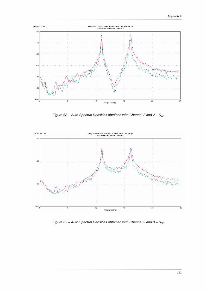
Appendix F
111
Figure 68 – Auto Spectral Densities obtained with Channel 2 and 2 – S22
Figure 69 – Auto Spectral Densities obtained with Channel 3 and 3 – S33

Seismic Vulnerability Assessment of Structures using Operational Modal Analysis
112
Figure 70 – Cross Spectral Densities obtained with Channel 1 and 2 – S12 or S21
Figure 71 – Cross Spectral Densities obtained with Channel 1 and 3 – S13 or S31

Appendix F
113
Figure 72 – Cross Spectral Densities obtained with Channel 2 and 3 – S23 or S32
On the other hand the eigenfrequencies can also be determined through peak picking directly
from the plot of singular values which can be calculated from the singular value matrix Σ of the
singular value decomposition algorithm.