Seismic surveys
214
Planning Land 3-D Seismic Surveys Andreas Cordsen, Mike Galbraith, and John Peirce Edited by Bob A. Hardage Series Editor: Stephen J. Hill Geophysical Developments Series No. 9 Society of Exploration Geophysicists
-
Upload
emilia-pop -
Category
Science
-
view
380 -
download
11
Transcript of Seismic surveys

Planning Land 3-D Seismic Surveys
Andreas Cordsen, Mike Galbraith, and John Peirce
Edited by Bob A. HardageSeries Editor: Stephen J. Hill
Geophysical Developments Series No. 9Society of Exploration Geophysicists

SOCIETY OF EXPLORATION GEOPHYSICISTS
Library of Congress Cataloging-in-Publication Data
Cordsen, Andreas.Planning land 3-D seismic surveys / by Andreas Cordsen, Mike Galbraith, and John
Peirce ; editor, Bob A. Hardage.p. cm.-- (Geophysical developments series ; no. 9)
Includes bibliographical references and index.ISBN 1- 56080-089-5 (vol.)
1. Seismic prospecting. I. Galbraith, Mike. II. Peirce, John. III. Hardage, BobAdrian, 1939- IV. Title. V. Geophysical development series ; v. 9.
TN269.8 .C67 2000622’.1592--dc21
00-026159
ISBN 0-931830-41-9 (Series)ISBN 1-56080-089-5 (Volume)
Society of Exploration GeophysicistsP.O. Box 702740Tulsa, OK 74170-2740
©2000 Society of Exploration GeophysicistsAll rights reserved. This book or parts hereof may not be reproduced in any form withoutwritten permission from the publisher.
Printed in the United States of America

Acknowledgments
The authors wish to acknowledge the contributions from the staff members of GeophysicalExploration & Development Corporation and Seismic Image Software Ltd., both of Calgary,Alberta, Canada.
Several other individuals made significant contributions to this volume: in particular, PeterEick of Conoco, who added a lot of practical perspective (and photographs), Gijs J. O. Vermeerof 3DSymSam, and Malcolm Lansley of Western Geophysical, who reviewed the text at an ear-lier stage and had many suggestions, which, in part, have been incorporated.
We also thank the people who have taken our 3-D design courses and who have contributedto this book through their numerous discussions with us. With their help, many aspects of 3-Ddesign became more clearly understood.
iii

Introduction
This book is intended to give readers the tools tostart designing 3-D seismic surveys. The substantialexperiences of the authors in designing and acquiringland 3-D seismic surveys make this a practical book.
Readers are expected to have a general workingknowledge of 2-D seismic data acquisition, process-ing, and interpretation. Some 3-D experience is help-ful but not necessary to understand this material.Practical exercises are included to facilitate under-standing of the subject matter.
Throughout this book, an attempt has been made toprovide data examples in both metric and imperialunits. The imperial examples are shown in italics andare not necessarily a straight conversion from the met-ric examples, but rather are parameter values that arein common usage.
Some geophysicists may want to enhance theirknowledge of 3-D design by reading papers concern-ing their particular special interests. A reference listand a collection of other recommended reading areprovided at the end of the book.
iv

Abbreviations
The commonly used abbreviations listed here willbe used in this text. Other abbreviations may be usedthroughout the text and are explained when used.
B bin dimensionBr in-line bin dimension (receiver direction)Bs cross-line bin dimension (source direction)f frequencyfdom dominant frequencyfmax maximum frequencyk velocity factor (increase of velocity with
depth)K wavenumberMA migration apronNC number of channelsNRL number of receiver linesNSL number of source linesp ray parameterRF radius of first Fresnel zoneRI receiver intervalRLI receiver line intervalSD source density or number of source points
per unit area
SI source intervalSLI source line intervalt two-way traveltimeT period; temporal wavelengthU unit factorVave average velocity from surface to the reflect-
ing horizonVint interval velocity immediately above the re-
flecting horizonV0 velocity at surfaceVz velocity at depth ZXmax maximum recorded offsetXmin largest minimum offsetXmute depth varying mute distanceXr in-line dimension of the patchXs cross-line dimension of the patchZ depth to reflecting horizon� wavelength�dom dominant wavelength�max maximum wavelength� geologic dip angle�o take-off angle
v

vi
Conversion Tables
To convert from imperial units to metric units multiply by
Inches (in) Centimeters (cm) 2.54Feet (ft) Meters (m) 0.3048Miles (mi) Kilometers (km) 1.609Square miles (mi2) Square kilometers (km2) 2.56Acres (ac) Hectares (ha) 0.405Barrels (bbls) Cubic meters (m3) 0.159Thousand cubic feet gas (mcf) Thousand cubic meters (103m3) 0.028169Pounds (lb) Kilograms (kg) 0.454
To convert from metric units to imperial units multiply by
Centimeters (cm) Inches (in) 0.3937Meters (m) Feet (ft) 3.28Kilometers (km) Miles (mi) 0.6215Square kilometers (km2) Square miles (mi2) 0.39Hectares (ha) Acres (ac) 2.47Cubic meters (m3) Barrels (bbls) 6.29Thousand cubic meters (103m3) Thousand cubic feet gas (mcf) 35.5Kilograms (kg) Pounds (lb) 2.2
To convert to multiply by
Thousand cubic feet gas (mcf) Barrel of oil equivalent (boe) 0.1Miles (mi) Feet (ft) 5280Square miles (mi2) Acres (ac) 640Square miles (mi2) Hectares (ha) 256Hectares (ha) Square meters (m2) 10 000

Table of Contents
CHAPTER 1 INITIAL CONSIDERATIONS
1.1 Management Attitudes 1
1.2 Objectives 1
1.3 Industry Trends 2
1.4 Financial Issues 2
1.5 Target Horizons 5
1.6 Sequence of Events for Data Acquisition 5
1.7 Environment and Weather 8
1.8 Special Considerations of 3-D versus 2-D Data Acquisition 8
1.9 Definitions of 3-D Terms 8
Chapter 1 Quiz 12
CHAPTER 2 PLANNING AND DESIGN
2.1 Survey Design Decision Table 13
2.2 Orthogonal Geometry 14
2.3 Fold 14
2.4 In-line Fold 16
2.5 Cross-line Fold 17
2.6 Total Fold 18
2.7 Fold Taper 19
2.8 Signal-to-Noise Ratio (S/N) 20
2.9 Bin Size 20
2.9.1 Target Size 21
2.9.2 Maximum Unaliased Frequency 21
2.9.3 Lateral Resolution 24
2.9.3.1 Lateral Resolution after Migration 25
2.9.3.2 Separation of Diffractions 26
2.9.4 Vertical Resolution 27
Let’s Design a 3-D—Part 1 28
2.10 Xmin 29
2.11 Xmax 32
2.11.1 Target Depth 34
2.11.2 Direct Wave Interference 34
2.11.3 Refracted Wave Interference (First Breaks) 35
2.11.4 Deep Horizon Critical Reflection Offset 35
2.11.5 Maximum NMO Stretch to Be Allowed 35
2.11.6 Required Offset to Measure Deepest LVL (refractor) 35
2.11.7 Required NMO Discrimination 35
2.11.8 Multiple Cancellation 35
2.11.9 Offsets Necessary for AVO 35
2.11.10 Dip Measurements 35
vii

Let’s Design a 3-D—Part 2 36
Chapter 2 Quiz 37
CHAPTER 3 PATCHES AND EDGE MANAGEMENT
3.1 Offset Distribution 39
3.2 Azimuth Distribution 40
3.3 Narrow versus Wide Azimuth Surveys 40
3.4 85% Rule 41
3.5 Fresnel Zone 46
3.6 Diffractions 47
3.7 Migration Apron 47
3.8 Edge Management 48
3.9 Ray-Trace Modeling 51
3.10 Record Length 51
Let’s Design a 3-D – Part 3 53
Let’s Design a 3-D – Summary 54
Chapter 3 Quiz 55
CHAPTER 4 FLOWCHARTS, EQUATIONS, AND SPREADSHEETS
4.1 3-D Design FlowChart 57
4.2 Basic 3-D Equations—Square Bins 57
4.3 Basic 3-D Equations—Rectangular Bins 59
4.4 Basic Steps in 3-D Layout—Five-Step Method 59
4.5 Graphical Approach 61
4.6 Standardized Spreadsheets 62
4.7 Estimating the Cost of a 3-D Survey 69
4.8 Cost Model 69
CHAPTER 5 FIELD LAYOUTS
5.1 Full-Fold 3-D 77
5.2 Sampling the 5-D Prestack Wavefield 77
5.3 Swath 81
5.4 Orthogonal 81
5.5 Brick 83
5.6 Nonorthogonal 83
5.7 Flexi-Bin® or Bin Fractionation 85
5.8 Button Patch 89
5.9 Zig-Zag 91
5.10 Mega-Bin 92
5.11 Hexagonal Binning 93
5.12 Star 96
viii Table of Contents

5.13 Radial 96
5.14 Random 96
5.15 Circular Patch 99
5.16 Nominal Fold Comparison 99
Chapter 5 Quiz 105
CHAPTER 6 SOURCE EQUIPMENT
6.1 Explosive Sources 107
6.2 Dynamite Testing 113
6.3 Dynamite Shooting Strategy 113
6.4 Vibrators 113
6.5 Vibrator Array Concepts 114
6.6 Vibrator Testing 116
6.7 Vibrator Deployment Strategy 118
6.8 Other Sources 119
Chapter 6 Quiz 119
CHAPTER 7 RECORDING EQUIPMENT
7.1 Receivers 121
7.2 Recorders 123
7.3 Distributed Systems 124
7.4 Telemetry Systems 126
7.5 Remote Storage 127
Chapter 7 Quiz 127
CHAPTER 8 ARRAYS
8.1 The Question of Arrays 129
8.2 Geophone Arrays 129
8.3 Source Arrays 131
8.4 Combined Array Response 131
8.5 Stack Arrays 131
8.6 Hands-Off Acquisition Technique 134
8.7 Symmetric Sampling 134
CHAPTER 9 PRACTICAL FIELD CONSIDERATIONS
9.1 Surveying 135
9.2 Script Files 138
9.3 Templates 141
9.4 Roll-On/Off 141
Table of Contents ix

9.5 No Roll-On/Off 142
9.6 Swath Width 142
9.7 Shooting Strategy 143
9.7.1 Vibrator 145
9.7.2 Dynamite 146
9.8 Large Surveys 146
9.9 Field Visits (QC) 147
9.10 Offsets and Skids 148
9.11 General Considerations 148
9.11.1 Imaging Area 148
9.11.2 Cables 149
9.11.3 Permitting 150
9.11.4 Safety 150
9.12 Field Examples 151
9.13 Field QC (Data) 152
9.13.1 Positional Data Quality 152
9.13.2 Seismic Data Quality 152
9.13.3 Verify Seismic/Positional Data Relationship 153
Chapter 9 Quiz 155
CHAPTER 10 PROCESSING
10.1 Processing 157
10.2 Processing Stream 157
10.3 Refraction Statics 158
10.4 Velocity Analysis 158
10.5 Reflection Statics 161
10.6 Dip Moveout 162
10.7 Stack 166
10.8 Acquisition Footprints 166
10.9 Migration and Random Sampling 167
10.10 Making Adjustments for Data Quality 168
Chapter 10 Quiz 169
CHAPTER 11 INTERPRETATION
11.1 Interpretation Systems 171
11.2 Mapping 171
11.3 Integration 172
11.4 Acquisition Footprints 173
11.5 Seismic Attributes 173
11.6 Geostatistics 173
11.7 Immersion Technology 173
x Table of Contents

CHAPTER 12 SPECIAL INTEREST TOPICS
12.1 Digital Orthomaps and GIS data 17512.2 Transition Zones 17512.3 Presstack Time and Depth Migration 17612.4 Time-Lapse (4-D) Seismic 17712.5 Converted Wave 3-D Design 17712.6 3-D Inversions 18012.7 Future Directions 181
ANSWERS TO QUIZ QUESTIONS 183
GLOSSARY 185
REFERENCES 195
INDEX 201
Table of Contents xi

1.1 MANAGEMENT ATTITUDES
The management of an oil company needs to be fa-miliar with the acquisition, processing, and interpre-tation requirements that a 3-D survey may place on itsstaff. If a company’s management has had prior expo-sure to 3-D seismic surveys, less education by thetechnical staff (usually the geophysicists) is necessarybefore recommending a 3-D survey. There may besome preconceived ideas as to the final products thatmight be delivered at various stages. It is important toemphasize that success or failure in a past 3-D surveymay not necessarily be duplicated in future programs.Modifying the design, acquisition, and processing pa-rameters can make significant improvements. Con-versely, results may be less than expected if poor de-sign parameters are chosen.
Geophysicists may find themselves serving one ormore customers. Once 3-D data have been acquiredand interpreted, the interpreted data set will become afocal point for several people because the interpreta-tion will be delivered to team members that practicedifferent disciplines (Figure 1.1). The data also be-come a valuable asset with resale value.
Possible partners may need to be informed at anearly stage about the planned operations so they canset aside the anticipated financial and personnel resources. They may wish to have significant inputinto choosing the area for the 3-D survey, or in planning the design, or they may wish to contributein some other manner. Obtaining their approval ismuch easier if they have been intimately involvedfrom the start. This approach gives partners a sense of ownership. Sometimes the company that operatesthe field is not the one that contributes most to a 3-D survey. It is possible, for example, that anotherpartner in the area could operate an extensive seismicprogram. Information exchange is an important as-
pect of doing the very best technical job in 3-D designand acquisition.
1.2 OBJECTIVES
A company needs to establish early and clearly whya 3-D survey is to be recorded (some possible reasonsare listed in Figure 1.2). These goals must be kept in mind during all phases of the planning process.Any seismic program must be planned, recorded,processed, and interpreted in time to deliver sufficientresults to the owners of the data so that they can eval-uate all results along with other information and con-straints that they may have.
Most of the reasons for recording the 3-D seismicdata listed in Figure 1.2 do not need any explanations.
1
1Initial Considerations
Fig. 1.1. The geophysicist as part of the exploration/exploitation team.
©2000 Society of Exploration Geophysicists. All rights reserved.

For example, reservoir monitoring may be essentialfor better production practices in large fields. The dif-ferences observed in 3-D seismic surveys recordedover the same field with a separation period of severalyears show the progress of depletion and floodingpractices. Such “4-D” or “time-lapse” surveys are be-coming more common.
1.3 INDUSTRY TRENDS
Both large and small companies now use high-tech-nology tools to obtain data improvements. This prac-tice is particularly true for the energy sector, espe-cially regarding the use of 3-D seismic technology.Success ratios for oil companies have been increasedby using 3-D data. In a worldwide study, one largecompany registered an increase in their success ratefrom 13% in 1991 using 2-D data to 44% in 1996 using3-D technology extensively (Ayler, 1997). While thesuccess rate using 2-D data alone has remained con-stant, the success rate using 3-D seismic technologyhas shown a dramatic improvement.
Small independent companies may acquire small 3-D surveys to help detail relatively small land holdingssurrounding existing production. Larger oil compa-nies may acquire 3-D data over larger areas of 10s or100s of km2. Often these surveys are for exploratorypurposes only. One important new trend is that acqui-sition contractors are now offering to record huge 3-Dparticipation surveys not only in the offshore environ-ment where the practice has been done for a while,but also onshore.
One estimate for North America indicates that bythe year 2007, essentially all of the area in the US andCanada that is suitable for the application of 3-D seis-mic technology will be covered (Figure 1.3). Since thisis an average estimate, there will be many areas thatwill be covered more than once by a 3-D survey with-out the intention of doing 4-D surveys. With acquisi-tion prices falling at a fast rate and higher channel ca-pacities being available, 3-D acquisition becomes thefavored choice over 2-D acquisition.
Many major oil companies have the necessary re-sources and expertise to plan, acquire, process, and interpret 3-D data in-house, while medium andsmall-size oil companies rely on the knowledge andexperience that consultants offer. By constantly deal-ing with the subject of 3-D data acquisition, it is mucheasier to be proficient at planning and operating suchsurveys.
1.4 FINANCIAL ISSUES
Cost factors play an important role in making deci-sions about the expenditures for a 3-D survey. The ex-ploration team must prove to management that adense grid of geophysical data tied to geological in-formation from existing wells provides significanteconomic benefits by reducing the number of dryholes and overall costs. In the past, at least one dis-covery well in a particular prospect area was needed
2 Initial Considerations
Fig. 1.2. Different reasons for shooting a 3-D seismic survey.
3-D
su
itab
le a
rea (
% s
ho
t)
200720031999
Rapid Growth
Slow Growth
199519911987
100
90
80
70
60
50
40
30
20
10
0
Fig. 1.3. Application of 3-D seismic technology to areassuitable for 3-D data acquisition in North America (Koen,1995 after A. Cranberg, Aspect Management Corp.).
©2000 Society of Exploration Geophysicists. All rights reserved.
to convince management to spend additional re-sources on 3-D seismic data. Recently there has been atrend to use 3-D technology even in a purely ex-ploratory environment. The cost of acquiring several2-D programs possibly spread over many years maybe just as high as a 3-D survey. In addition, the prob-lems of interpreting and consistently incorporatingvarious vintages of 2-D data lead to inevitable uncer-tainties that may be insurmountable. Therefore, ac-quiring 3-D seismic data provides a more cost-effec-tive evaluation of a prospect by providing increasedconfidence in the seismic interpretation and new tech-nical information.
Budget constraints need to be made clear at theearly planning phase; otherwise, unrealistic designsmay result. If the budget numbers are too low, the 3-Dsurvey may be under-designed and unable to meetmanagement expectations. On the other hand, if thebudget numbers are too high, the designers of the 3-Dsurvey may over-design in areal extent or in othertechnical specifications. Important considerations are:who ultimately controls the budget; who approvesany unanticipated changes, especially cost overruns;does the planning committee meet on particular datesor at irregular intervals; and how difficult is it to ob-tain timely approvals in order to maintain the timeschedule?
Management needs to be able to evaluate the eco-nomic rate of return for any project in question. Thepotential of a prospect and its associated risk mustwarrant the cost of a 3-D seismic survey. More oftenthan not, a 3-D survey is difficult to justify on a single-well basis. However, a 3-D seismic survey may verywell be worthwhile if dry holes are to be avoided. Ex-ploration wildcat wells are commonly that type of sit-uation. A 3-D survey may make a wildcat less “wild”and result in the drilling of significant discoveries.The cost of missed opportunities is very high.
On a project that has numerous development loca-tions, and even for low-cost drilling of relatively shallow wells, 3-D seismic surveys are often eco-nomically justifiable. If many step-out wells and in-fill locations are anticipated, project economics maydictate a 3-D survey. Similarly, plans for horizontaldrilling may require tightly controlled seismic data.For example, if the target horizon is relatively thin,drilling engineers may need high-resolution sam-pling in all three dimensions to keep the drill bit inthe reservoir.
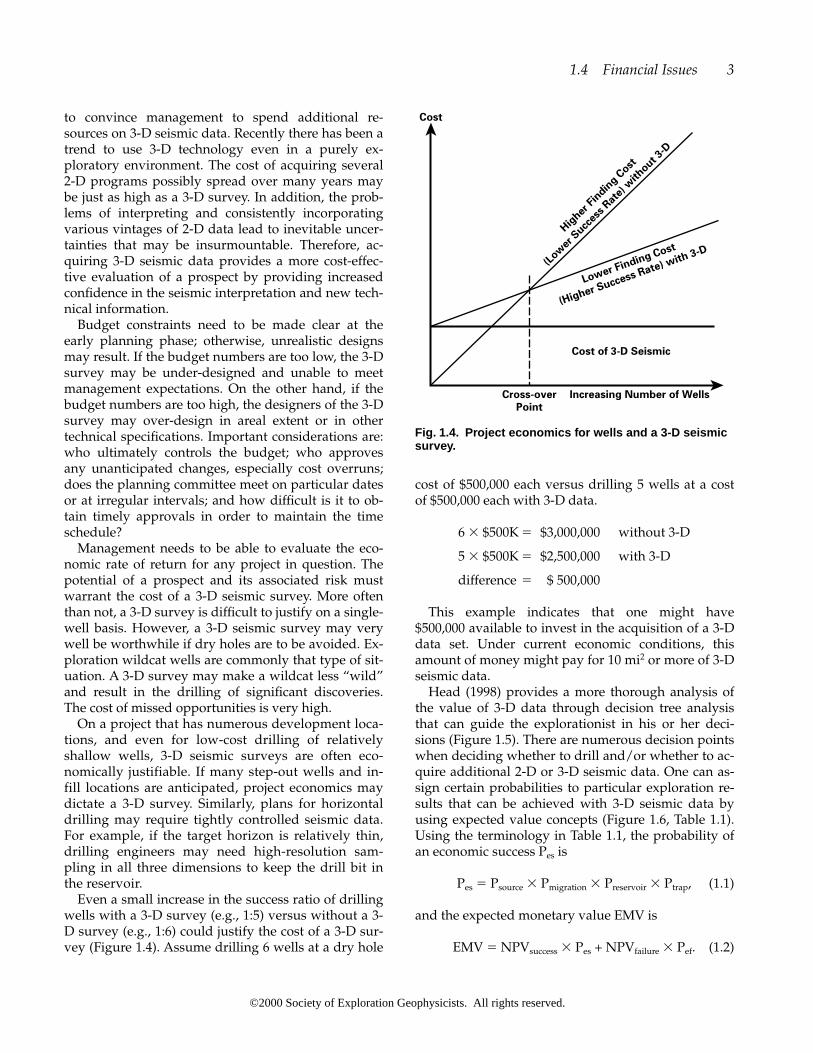
Even a small increase in the success ratio of drillingwells with a 3-D survey (e.g., 1:5) versus without a 3-D survey (e.g., 1:6) could justify the cost of a 3-D sur-vey (Figure 1.4). Assume drilling 6 wells at a dry hole
cost of $500,000 each versus drilling 5 wells at a costof $500,000 each with 3-D data.
6 � $500K � $3,000,000 without 3-D
5 � $500K � $2,500,000 with 3-D
difference � $ 500,000
This example indicates that one might have$500,000 available to invest in the acquisition of a 3-Ddata set. Under current economic conditions, thisamount of money might pay for 10 mi2 or more of 3-Dseismic data.
Head (1998) provides a more thorough analysis ofthe value of 3-D data through decision tree analysisthat can guide the explorationist in his or her deci-sions (Figure 1.5). There are numerous decision pointswhen deciding whether to drill and/or whether to ac-quire additional 2-D or 3-D seismic data. One can as-sign certain probabilities to particular exploration re-sults that can be achieved with 3-D seismic data byusing expected value concepts (Figure 1.6, Table 1.1).Using the terminology in Table 1.1, the probability ofan economic success Pes is
Pes � Psource � Pmigration � Preservoir � Ptrap, (1.1)
and the expected monetary value EMV is
EMV � NPVsuccess � Pes + NPVfailure � Pef. (1.2)
1.4 Financial Issues 3
Cost
Cross-overPoint
Cost of 3-D Seismic
Lower Finding Cost
(Higher Success Rate) with 3-D
Hig
her F
indin
g Cost
(Low
er S
ucces
s Rat
e) w
ithout 3
-D
Increasing Number of Wells
Fig. 1.4. Project economics for wells and a 3-D seismicsurvey.
©2000 Society of Exploration Geophysicists. All rights reserved.

Through such analysis one can establish the maxi-mum economic value to ascribe to a 3-D seismic sur-vey. The difference in the expected monetary value(EMV) of the project without and with 3-D data deter-mines the maximum amount that can be spent on a 3-D survey. Total project economics, cost of money, anda possible increase or decrease in the total projectNPV are not taken into account in Figure 1.6. Aylor(1995) points out that many 3-D surveys add value toexploration and development projects because morewells can be drilled.
Costs for 3-D surveys vary depending on the areawhere the survey is to be conducted, the availabilityof equipment and crews, and the complexity of thegeography. In general, one can expect to pay on theorder of $10 000 to $50 000 per km2 for data acquisi-tion. High-resolution work for smaller bins and high-fold surveys can exceed those costs. On the otherhand, sparse 3-D surveys (Bouska, 1995) or very fo-
cused 3-Ds (Servodio et al., 1997) can provide costsavings. An analysis of the economics of different ac-quisition parameters is essential in evaluatingwhether high S/N ratios and small bin sizes are war-ranted. Such analysis is possible by decimating exist-
4 Initial Considerations
Table 1.1 Profitability Table
w/o 3-D with 3-D % change
Psource Probability of hydrocarbon source 90% 90% 0%Pmigration Probability of migration of hydrocarbons 80% 80% 0%Preservoir Probability of reservoir/porosity 70% 80% 14%Ptrap Probability of seal/trap 30% 40% 33%NPVsuccess Net present value of successful well $8,000,000 $8,000,000NPVfailure Net present value of dry well ($1,500,000) ($1,500,000)Pes Probability of economic success 15% 23% 52%Pef Probability of economic failure 85% 77% 9%EMV Expected monetary value ($63,600) $688,800VOI Value of information (e.g., 2-D, 3-D, interpretations) ($752,400)
Required success ratio for single well 16% 22% 39%
Fig. 1.5. Decision tree analysis to guide the explorationdecision process.
Fig. 1.6. Probability of economic success (P es) versusnet present value (NPV).
©2000 Society of Exploration Geophysicists. All rights reserved.

ing data sets and interpreting the individual data setsseparately (Schroeder and Farrington, 1998).
Processing costs vary but are usually in the range of5–10% of acquisition. A detailed interpretation shouldbe in the same cost range as processing.
1.5 TARGET HORIZONS
A 3-D seismic survey should be designed for themain zone of interest (primary target). This zone willdetermine project economics by affecting parameterselection for the 3-D seismic survey. Fold, bin size,and offset range all need to be related to the main tar-get. The direction of major geological features, such asfaults or channels, may influence the direction of thereceiver and source lines.
Secondary zones or other regional objectives mayhave a significant impact on the 3-D design as well. Ashallow secondary target, for example, may requirevery short near offsets. Deeper regional objectives andmigration considerations may dictate that the far off-set of the survey be substantially greater than themaximum stacking offset used in the fold calculationat the target level (Figure 1.7).
1.6 SEQUENCE OF EVENTS FOR DATAACQUISITION
Preparing an overall time line for data acquisitionwill avoid surprises and keep expectations somewhatclose to reality. This time planning should also help in
meeting critical deadlines such as land sales, lease ex-pirations, or bid submission dates. The technical teamshould update this time line as the project progresses,so that the parties involved are kept abreast of thechanges. A realistic time line needs to be establishedearly so that expectations are on track with the overallprocess of obtaining the data (Figure 1.8). The time re-quired for each step in the time line varies widelyfrom area to area. A small 3-D survey can be com-pleted from scouting to drilling within 6 to 8 weeks,while larger surveys in difficult access areas may de-mand two years or more. In-depth knowledge of localtime requirements is essential.
A scouting trip to the 3-D area may provide sub-stantial information for the design of the 3-D survey;e.g., existing cut lines may dictate line intervalsand/or direction, or surface cover could influence dynamite hole depth and charge size. All technical parameters must be kept in mind when designing a
1.6 Sequence of Events for Data Acquisition 5
Fig. 1.7. Primary target horizon versus secondary targets. Fig. 1.8. Time line of a 3-D seismic program.
©2000 Society of Exploration Geophysicists. All rights reserved.

survey. The design may need to be updated as moreelements and parameters of the time line becomeknown. Operators should request all necessary regu-latory approvals and stay in close contact with regula-tory bodies to ensure smooth operation, rememberingto consider past survey requirements and costs suchas forestry regulations, damages, reseeding, and cor-rection of erosion problems.
Critical questions such as “Are experienced 3-Dcrews available locally?” need to be answered early inthe project. If crews need to be shipped across thecountry or even from another country or continent,major delays should be expected, especially whenclearing customs. Some 3-D seismic equipment is of-ten hard to get through customs because officials of-ten do not understand the technology. Knowing theavailability of spare parts is important if anythinggoes wrong in the field. For example, if cables becomedamaged, how much replacement equipment can bebrought in and how long will it take?
Other key questions that need to be considered are:What kinds of data acquisition bid procedures arecustomary at the prospect location? How much timeis involved from requesting such bids to their actualsubmission? How much time do the contractors needto put a reasonably accurate bid together? Do contrac-tors need to research local conditions, and to what ex-tent? The oil company may have bidding procedureslaid out in a very particular manner, e.g., bids mayneed to be presented in a form of cost/km2,cost/source point, cost/day, or total project cost, justto name a few variations. The content requirementsfor an acquisition bid should be clearly known toeveryone involved in the bidding process. If the con-tractor has to sign a standard contract before embark-ing on a job, the oil company may want to include thiscontract at the stage of requesting a bid. It is impor-tant to negotiate a satisfactory contract that meets theneeds of the oil company’s particular situation andthat also reflects the political environment.
Many acquisition contractors will subcontract partsof the job such as surveying, shot-hole drilling, andbulldozer work. The costs of these subcontracts areusually considered extras and therefore may not beincluded in the overall cost/unit basis. A best effortmust be made to estimate the extent of these extras toarrive at a realistic total cost figure for a 3-D seismicsurvey. These so-called extras may more than doublethe acquisition cost. The uncertainties in cost becauseof allowances for bad weather can also represent asignificant portion of the total cost.
Turnkey quotes help set the price for most of the ac-quisition costs. This bidding policy assures a client
that the crew will work fast. Some element of supervi-sion must be introduced to obtain the required qualityof service. Daily rates, on the other hand, do not givethe crew an incentive to work fast. However, if noother jobs are waiting for the crew, the best level ofservice possibly can be obtained via a daily rate op-tion.
Some companies may choose to hire an acquisitioncrew for an entire acquisition season or even for sev-eral years. Under such circumstances, the need to ne-gotiate every seismic program disappears and betterplanning needs to be implemented for continuous op-eration. The price guarantee that usually accompaniessuch arrangements is a big advantage over the uncer-tainties that industry experiences in fluctuating mar-kets.
Often the legal contract that a contractor provides isnot comprehensive. If any field problems, accidents,or insufficiencies arise, an incomplete contract maylimit the legal protection for the acquisition contractorand the client. It is advisable to have legal representa-tives review the contract and ensure that sufficientprotection exists for both parties. If experience withsuch contracts does not exist within the organization,then outside advice should be requested.
Permits may be required from land surface ownersto obtain entry. Such permits should be requested asearly as possible because permit issues can affect a 3-D survey in a number of different ways. Permittingmay need to be started significantly earlier in the timeline of Figure 1.8. Landowners may not want to seeany member of an acquisition crew during the grow-ing season, even if crop damages are to be paid. Slightchanges in the design or layout of the receivers andsources may make a huge difference to particularlandowners. For example, by moving a portion of aline across the fence to neighboring noncrop land, onemay avoid crop damages and pay another landownerpermit fees. This is a beneficial scenario for all con-cerned. Good rapport with landowners will go a longway to assuring access to their lands, and keepingdamages to a minimum will help the next seismiccrew that wants to work in the same area. Often per-mitting by km2 is less expensive than permitting byline km. Permitting by area also gives more freedomof choice in the field.
If a landowner controls a high percentage of thelands within a 3-D survey and is opposed to the seis-mic operation, the entire program may be in jeopardy.Large gaps of “no coverage” on a 3-D survey are un-desirable, and such opposition may cripple theplanned survey and perhaps cancel part of the explo-ration program.
6 Initial Considerations
©2000 Society of Exploration Geophysicists. All rights reserved.

In at least one U.S. state (e.g., Texas), it is illegal torecord a geophysical measurement of any kind over an-other owner’s mineral rights without a permit from thatowner (geophysical trespass). There is considerable con-fusion as to how the relevant laws should be inter-preted. Most operators are now being diligent to obtainpermits over all relevant lands to protect themselvesagainst possible liability. Many operators of 3-D surveysare trimming their surveys to ensure that there are nostacked traces over areas not covered by permits (e.g.,not undershooting corners). Interested readers shouldsee AAPG Explorer, June 1995, for a discussion of theBurr Ranch case and related issues.
Key questions to consider include the following:How much is known about the operating conditions?Which contractors have experience in the area to con-tribute to the successful operation of such programs?Will the contractor share this information at the timeof bid submission or only if they win the contract?
If the knowledge of local operating conditions islimited or data quality to be expected is unknown,then a 2-D test line may be required and is sometimesessential for correct parameter selection. Source andreceiver array tests are much easier to conduct, espe-cially for small 3-D surveys, when a 2-D test line is be-ing considered as a first evaluation of the prospect.On a large 3-D survey, it might be justified to conductthe required tests at the start of the survey. Large sur-veys may require a variety of sources or receivers(such as in a transition zone), and several test se-quences may be performed throughout the survey.Sometimes the local conditions are known wellenough that a 3-D survey may proceed without anytesting at all.
Surveyors need to go to the field and establish aperimeter of the 3-D seismic survey before filling inthe specific source and receiver lines. Global Position-ing Systems (GPS) technology provides good surveyaccuracy and is a faster surveying technique thanmore traditional Electronic Distance Measurement(EDM) devices. Differential GPS, which relies on awell-established local base station, offers even greateraccuracy; its horizontal accuracy is �1 m while thevertical accuracy is 2 to 3 m presently. Accuracies of afew centimeters can be achieved with longer time oneach station. Once the grid has been established,chainers will mark every source and receiver group lo-cation. GPS does not work well in dense tree cover or indeep ravines where satellites cannot be seen. For fur-ther GPS information, see Harris and Longaker (1994).
Shot-hole drilling may commence immediately fol-lowing, or even concurrent with, the surveying. Usu-ally the entire 3-D area will be drilled before the
recording crew arrives, assuming that all source para-meters have been previously established. This drillingschedule reduces noise interference between thedrilling units and the data recording. There is also nochance of the drillers being in the way of the layoutcrew.
Vibrator trucks or buggies may start sweep produc-tion once the sweep parameters have been tested. It isalways advisable to complete phase, peak force, andcorrelation tests before going into production mode.These tests should be repeated several times duringthe acquisition program and should be done morethan once daily.
If a program does not allow or warrant any testing,an attempt should be made to find past tests or data.Testing is important for both dynamite and vibrator(or any other source) data acquisition. Such tests maybe instructive for any future programs, even if thepresent survey cannot benefit from the test results.
The recording crew places receivers on the groundin a predetermined array. The geophones are con-nected in receiver groups, which then transmit thedigital information in a variety of ways to therecorder. Cable-based distributed recording systemsrequire a continuous cable connection from the geo-phones to the recorder, thus one can walk out the ca-ble connections from any geophone all the way backto the recording truck. An alternate technique for datatransmission is the telemetry system, which uses ra-dio signals to transmit data to the recording truck in-stead of cables. In the case of the I/O RSR system,data are recorded locally and then retrieved periodi-cally for storage on tape. For this system, the radio isa control unit for initiation of recording and qualitycontrol, but it is not used for data transmission.
The recorder unit (dog house) has a complete set ofelectronics that allows data correlation (for vibrators)and the recording and display of shot records thatshow traces corresponding to all geophone groups.
Some crews operate on a 24-hour basis to reducethe overhead cost per source point. One has to checkwhether local customs and/or laws and safety con-cerns allow such around-the-clock operation. Limitingdata-recording activity to dawn-to-dusk significantlylengthens the number of days needed to record a 3-Dseismic survey.
Field tapes are sent to the processor for analysis andimaging of the data, or more recently, the data can beprocessed in the field. The choice of the processorshould be decided before the crew enters the field.Survey notes need to be reduced to final coordinates,and the final survey geometry must be forwarded tothe processor.
1.6 Sequence of Events for Data Acquisition 7
©2000 Society of Exploration Geophysicists. All rights reserved.

Interpretation on paper and/or on a workstationusually gives a clear idea of the geological variationsin the area of the 3-D survey. Drilling of explorationor development wells should commence only aftersufficient time has been allotted for a thorough andcomplete interpretation.
1.7 ENVIRONMENT AND WEATHER
Environmental issues play an important role in to-day’s world—especially in seismic data acquisition.One should protect the environment as much as pos-sible during all field operations. Line cutting inforested areas should be limited to the smallest widthnecessary. Small jogs in the lines are often requestedto protect the pristine appearance of the woods and toprotect wild life. In mountainous areas or other diffi-cult terrain, helicopter support may be essential forshot-hole drilling or for laying receiver cables to mini-mize damaging effects on the environment.
Wildlife protection issues have to be addressedsuch as mating seasons and migration paths. In atransition zone, fish spawning might be a concern atcertain times of the year. In some parts of the world,rodents may chew cables and hinder successful datatransmission. The use of wooden pegs for station flagslessens the damage to farm equipment and animals,such as cows, which often chew station flags and ca-bles. Some areas are so environmentally sensitive thatlocal interest groups may lobby government officialsto prevent any seismic operation, or they may inter-fere directly with seismic or drilling operations. Re-cent trends in the environmental industry have showna recognition that stopping the seismic operations alsoeffectively stops oil and gas exploration; therefore,good community relations in advance of operationsare a wise investment in time and effort.
Weather conditions may constrain operation of aseismic program to certain times of the year. Rain orsnow may alter ground conditions to such a degreethat data quality is severely diminished. Crew move-ment may also be hindered. In cold climates, one maywant to wait for frost before laying out geophones toimprove the coupling of the geophone spikes to theground and to minimize surface damages. Snowcover may need to be removed to allow the frost toenter the ground rather than allowing the snow to actas an insulator. Often receiver lines need to be clearedseveral times if significant new snowfall occurs dur-ing crew operations. In warmer climates, extreme heatconditions may hinder the effectiveness of the crewpersonnel and may pose a serious safety hazard.
1.8 SPECIAL CONSIDERATIONS OF 3-DVERSUS 2-D DATA ACQUISITION
One needs to specify the objectives of a 3-D surveymore precisely than for a 2-D survey because the ac-quisition parameters are more difficult to change inmid-program. For example, with a 3-D survey (as op-posed to 2-D) much more line cutting is required inforested areas. This makes it harder to obtain ap-proval from regulatory bodies, and even when ap-proval is granted, one may be limited to using exist-ing cut lines or be restricted to hand-cut receiver lines,which can slow the operation. On a 3-D survey, theequipment stays on the ground much longer than in2-D data programs. This factor exposes 3-D equip-ment to more environmental, vehicular, weather,theft, and wildlife damage.
Spatial sampling in 3-D programs is usually muchcoarser than in 2-D programs (e.g., 20 to 40 m bins ina 3-D survey versus 5 to 15 m trace spacings in 2-Dsurveys). It is important to decide whether thiscoarser sampling is sufficient to resolve structuraldips and to properly image geological features. For 2-D lines, linear source and geophone arrays are thenorm. The effects that source-receiver azimuths haveon these geophone (or source) arrays is a topic of re-cent papers and research. There is no consensus yet inthe industry on the type of arrays to use in 3-D dataacquisition.
Finally, 3-D sources and receivers are laid out overan area, and 3-D recordings have an azimuthal ele-ment that is not present in 2-D efforts. Good az-imuthal distributions are usually, but not always, de-sirable. If any out-of-the-plane phenomenon exists ina 2-D profile, often one is unable to determine the di-rection of its cause. In contrast, 3-D migration has abetter chance of properly positioning such anomalies.
One can argue at length about various aspects of 3-D versus 2-D imaging. 3-D data have a common set ofacquisition and processing parameters over a largearea and therefore are easier to interpret than a seriesof 2-D lines of various vintages. A 3-D data volume iscontinuous, and one may extract profiles in any direc-tion out of this volume. However, in some situations,2-D data may be more beneficial than 3-D data, e.g.,when there is a need to gain a regional perspective orto improve local resolution with a small trace spacing.
1.9 DEFINITIONS OF 3-D TERMS
Figures 1.9 and 1.10 show a plan view of an orthog-onal 3-D survey that illustrates most of the terminol-ogy used in this book.
8 Initial Considerations
©2000 Society of Exploration Geophysicists. All rights reserved.

Note: This book uses SI notation as a standard;however, most numerical examples are presented inimperial units as well, and these are printed in italics.Rather than directly converting metric units to imper-ial units, we have chosen the natural imperial unitsthat would be used in the particular situation (e.g., a30 m bin size might be equivalent to a 110 ft bin size).
Box (sometimes called “Unit Cell”) In orthogonal3-D surveys, this term applies to the area bounded by two adjacent source lines and two adjacent re-ceiver lines (Figures 1.9 and 1.12). The box usuallyrepresents the smallest area of a 3-D survey that contains the entire survey statistics (within the full-fold area). In an orthogonal survey, the midpoint bin located at the exact center of the box has con-tributions from many source-receiver pairs; the shortest offset trace belonging to that bin has thelargest minimum offset of the entire survey. In other words, of all the minimum offsets in all CMP bins, the minimum offset in the bin at the center
1.9 Definition of 3-D Terms 9
Fig. 1.9. 3-D survey layout terms.
Fig. 1.10. 3-D survey bin terms.
of the box has the biggest Xmin. Different layout strate-gies attempt to deal with this concept in a variety of ways.
CMP Bin (or Bin) A small rectangular area that usu-ally has the dimensions (SI � 2) � (RI � 2). All mid-
©2000 Society of Exploration Geophysicists. All rights reserved.

points that lie inside this area, or bin, are assumed tobelong to the same common midpoint (Figure 1.10).In other words, all traces that lie in the same bin willbe CMP stacked and contribute to the fold of that bin.On occasion, one may choose the area over whichtraces are stacked to be different from the bin size inorder to increase stacking fold. This introduces somedata smoothing and should be performed with cau-tion because it affects spatial resolution.
Cross-line Direction The direction that is orthogo-nal to receiver lines.
Fold The number of midpoints that are stackedwithin a CMP bin. Although one usually gives one av-erage fold number for any survey, the fold varies frombin to bin and for different offsets.
Fold Taper The width of the additional fringe areathat needs to be added to the 3-D surface area to buildup full fold (Figure 1.11). Often there is some overlapbetween the fold taper and the migration apron be-cause one can tolerate reduced fold on the outer edgesof the migration apron.
In-line Direction The direction that is parallel to re-ceiver lines.
Midpoint The point located exactly halfway be-tween a source and a receiver location. If a 480-chan-nel receiver patch is laid out, each source point willcreate 480 midpoints. Midpoints will often be scat-tered and may not necessarily form a regular grid.
Migration Apron The width of the fringe area thatneeds to be added to the 3-D survey to allow propermigration of any dipping event (Figure 1.11). Thiswidth does not need to be the same on all sides of thesurvey. Although this parameter is a distance ratherthan an angle, it has been commonly referred to as themigration aperture. The quality of images achieved by3-D migration is the single most important advantageof 3-D versus 2-D imaging.
Patch A patch refers to all live receiver stations thatrecord data from a given source point in the 3-D sur-vey. The patch usually forms a rectangle of severalparallel receiver lines. The patch moves around thesurvey and occupies different template positions asthe survey moves to different source stations.
Receiver Line A line (perhaps a road or a cut-linethrough bush) along which receivers are laid out atregular intervals. The in-line separation of receiverstations (receiver interval, RI) is usually equal to twice
the in-line dimension of the CMP bin. Normally thefield recorder cables are laid along these lines andgeophones are attached as necessary. The distance be-tween successive receiver lines is commonly referredto as the receiver line interval (or RLI). The method oflaying out source and receiver lines can vary, but thegeometry must obey simple guidelines.
Scattering Angle Assuming the presence of a pointscatterer (diffraction point) at depth, the scattering an-gle is the angle between the vertical downgoingsource-scatterer raypath and the upgoing scatterer-re-ceiver raypath.
Signal-to-Noise Ratio The ratio of the energy of thesignal over the energy of the noise. Usually abbrevi-ated as S/N.
Source Line A line (perhaps a road) along whichsource points (e.g., dynamite or vibrator points) aretaken at regular intervals. The in-line separation ofsources (source interval, SI) is usually equal to twicethe common midpoint (CMP) bin dimension in thecross-line direction. This geometry ensures that themidpoints associated with each source point will fallexactly one midpoint away from those associatedwith the previous source point on the line. The dis-tance between successive source lines is usually calledthe source line interval (or SLI). SLI and SI determinethe source point density (or SD, source points persquare kilometer).
Source Point Density (sometimes called shot den-sity), SD The number of source points/km2 orsource points/mi2. Together with the number of chan-nels, NC, and the size of the CMP bin, SD determinesthe fold.
Super Bin This term (and others like macro bin ormaxi bin) applies to a group of neighboring CMPbins. Grouping of bins is sometimes used for velocitydetermination, residual static solutions, multiple at-tenuation, and some noise attenuation algorithms.
Swath The term swath, has been used with differentmeanings in the industry. First, and most commonly, aswath equals the width of the area over which sourcestations are recorded without any cross-line rolls. Sec-ond, the term describes a parallel acquisition geome-try, rather than an orthogonal geometry, in whichthere are some stacked lines that have no surface linesassociated with them.
Template A particular receiver patch into which anumber of source points are recorded. These source
10 Initial Considerations

points may be inside or outside the patch. In equationform,
Template = Patch � associated source points.
Xmax The maximum recorded offset, which dependson shooting strategy and patch size. Xmax is usuallythe half-diagonal distance of the patch. Patches withexternal source points have a different geometry. Alarge Xmax is necessary to record deeper events.
Xmin The largest minimum offset in a survey (some-times referred to as LMOS, largest minimum offset) asdescribed under “Box.” See Figure 1.12. A small Xmin
is necessary to record shallow events.Assuming RLI and SLI of 360 m (1320 ft), RI and SI
of 60 m (220 ft), the bin dimensions are 30 m � 30 m(110 ft � 110 ft). The box (being formed by two paral-lel receiver lines and the orthogonal source lines) hasa diagonal of:
Xmin � (3602 � 3602)1/2 m� 509 m
Xmin � (13202� 13202)1/2 ft
� 1867 ft
The value of Xmin defines the largest minimum off-set to be recorded in the bin that is in the center of thebox. In this example the source and receiver stations
are intentionally coincident at the line intersectionsfor simplicity.
Xmute The mute distance for a particular reflector.Any traces beyond this distance do not contribute to
1.9 Definition of 3-D Terms 11
Fig. 1.11. 3-D survey edge management terms.
Fig. 1.12. Xmin definition.

the stack at the reflector depth. Xmute varies with two-way traveltime.
Chapter 1 Quiz
1. Define receiver line interval.2. What is migration apron?
3. How does one determine Xmin in an orthogonalsurvey (orthogonal source and receiver lines)?
4. How large is a super bin?
12 Initial Considerations

Survey design depends on so many different inputparameters and constraints that it has become quitean art. Laying out lines of sources and receivers mustbe done with an eye toward the expected results. Asolid understanding of the required geophysical para-meters must be in place prior to embarking on a 3-Ddesign project (Kerekes, 1998). Some rules of thumband guidelines are essential to help one through themaze of different parameters that need to be consid-
ered. Computer programs are now available to assistin this task.
2.1 SURVEY DESIGN DECISION TABLE
Table 2.1 shares how to determine the values offold, bin size, Xmin, Xmax, migration apron, fold taper,and record length that should be incorporated into a
13
2Planning and Design
Table 2.1 Survey Design Decision Table.*
Parameter Definitions and Requirements
Fold Should be fold (if the S/N is good) up to 2-D fold (if high frequencies are expected).In-line fold � number of receivers � RI � (2 � SLI).Cross-line fold � NRL � 2.
Bin size Use 3 to 4 traces across target.Should be � Vint � (4 � fmax � sin � ); for aliasing frequency.Should provide N (� 2 to 4) points per wavelength of dominant frequency.Lateral Resolution available: � � N or Vint � (N � fdom ).
Xmin Should be less than 1.0 to 1.2 times depth of shallowest horizon to be mapped.
Xmax Should be approximately the same as target depth.Should not be large enough to cause direct wave interference, refracted wave interference (first
breaks), or deep horizon critical reflection offset, particularly in the cross-line direction, or intolera-ble NMO stretch.
Should exceed offset required to see deepest LVL (refractor), offset required to cause NMO �t> one wavelength of fdom , offset required to get multiple discrimination >3 wavelengths, and offset nec-essary for AVO analysis.
Should be large enough to measure Xmax as a function of dip.
Migration apron Must exceed radius of first Fresnel zone, diffraction width (apex to tail) for an upward scattering(full-fold) angle of 30°, i.e., Z tan 30° � 0.58 Z, and dip lateral movement after migration, which is Z tan �.
Can overlap with fold taper.
Fold taper Is approximately patch dimension � 4.
Record length Must be sufficient to capture target horizons, migration apron, and diffraction tails.
*The more important requirements are in italics. Additional definitions can be found in the Glossary.
12 � 2-D
©2000 Society of Exploration Geophysicists. All rights reserved.

design. These parameters constitute the key designfactors that need to be determined for a 3-D design.Each key parameter is discussed in this chapter and inChapter 3.
2.2 ORTHOGONAL GEOMETRY
Often source and receiver lines are laid out orthogo-nal to each other in onshore 3-D surveys. Such anarrangement is easy for survey and recording crewsto follow and keeping track of station numbering isstraightforward. Receiver lines could run east-westand source lines north-south, as shown in Figure 2.1,or vice versa. This method is easy to lay out in thefield and allows convenient equipment deploymentahead of shooting and roll-along operation. In thisgeometry, all source stations between adjacent re-ceiver lines are recorded, the receiver patch is rolledover one line (or several lines), and the process is re-peated. A portion of a 3-D layout is shown in Figure2.1a, and a detailed view is presented in Figure 2.1b.In Chapters 2, 3, and 4, discussions concentrate onthis layout method. Other methods that may be moresuitable for solving particular problems are describedin Chapter 5.
2.3 FOLD
Stacking fold (or fold-of-coverage) is the number offield traces that contribute to one stack trace, i.e., thenumber of midpoints per CMP bin. It is also the num-ber of overlapping midpoint areas (see Section 5.2).
Fold controls the signal-to-noise ratio (S/N). If thefold is doubled, a 41% increase in S/N is accom-plished (Figure 2.2). Doubling the S/N ratio requiresquadrupling the fold, assuming that the noise is dis-tributed in a random Gaussian fashion. Fold shouldbe decided by looking at previous 2-D and 3-D sur-veys in the area, through evaluating Xmin and Xmax
(Cordsen, 1995b), by modeling, and by rememberingthat dip moveout (DMO) and 3-D migration can effec-tively increase fold.
Krey (1987) showed that the ratio of 3-D to 2-D foldis frequency dependent and varies according to
3-D fold � 2-D fold � frequency � C, (2.1)
where C is an arbitrary constant.For example, if C � 0.01 and 2-D fold � 40, then 3-
D fold � 20 at 50 Hz and 40 at 100 Hz.
Rule of Thumb: Many designers use the equation, 3-D Fold 5 3 2-D Fold up to the 2-D Fold.
For example, if 2-D fold � 40, then a 3-D fold �
usually achieves comparable signal-to-noise results to the 2-D data. To be on the safe side(especially if one expects high frequencies; e.g., over100 Hz), one may define 3-D fold to be equal to the 2-D fold.
Some designers recommend that 3-D fold befold or even less. This lower ratio can give
acceptable results only if the area has excellent S/Nand only if there are minor problems with statics. Thethree-dimensional continuity of a 3-D data volume allows an easier correlation to neighboring lines than does 2-D data, hence a lower 3-D fold can be acceptable.
13 � 2-D
12 � 40 � 20
12
14 Planning and Design
Fig. 2.1a. Or thogonal survey design.
Fig. 2.1b. Orthogonal design—zoomed.
©2000 Society of Exploration Geophysicists. All rights reserved.

Krey’s (1987) more complete formula for 3-D fold is
3-D fold � 2-D fold
(2.2)
As an example, if 2-D fold � 30 then,
or
If the 2-D trace spacing is much smaller than the 3-D bin size, then 3-D fold must be relatively higher toachieve results comparable to the 2-D imaging. How-ever, large channel counts now mean that many 2-Dsurveys can be acquired with small trace spacing andlarge fold. Consequently many 2-D surveys are over-sampled with higher than required fold. One must al-ways keep this in mind when comparing 2-D and 3-Dfold. In further support of a lower 3-D fold, one mayconsider trace (or sampling) density rather than geo-phone station density. Larger numbers of geophonesper group certainly are sampling the subsurface moredensely, and may improve data quality, when all 24geophones are stacked into only one trace. However,24 geophones per group do not necessarily provide
3-D fold � 30 �1102 ft 2 � 50 Hz � � 0.4
55 ft � 15 000 ft/s� 28.
3-D fold � 30 �302 m2 � 50 Hz � � 0.4
20 m � 4500 m/s� 19
�3-D bin spacing2 � frequency � � 0.401
2-D CDP spacing � velocity.
better data than groups with 6 geophones. Similarlyfor sources, one may think of the sweep effort persquare kilometer, where sweep effort is defined ac-cording to the description in Chapter 6 [particularlyequation (6.2)].
There are many ways to calculate fold; the basic factis that one source point creates as many midpoints asthere are recording channels. If all offsets are withinthe acceptable recording range, then the basic foldequation is
Fold � SD � NC � B2 � U, (2.3a)
where SD is the number of source points per unitarea, NC is the number of channels, B is the bin di-mension (for square bins), and
U �
units factor (10–6 for m/km2; 0.03587 � 10–6 for ft/mi 2).
Derivation of equation (2.3a):
Number of midpoints � number of source points � NC
Source density
Combine to obtain
Survey size � Number of bins � bin size B2.
Multiply with prior equation
Example: Assuming that SD is 46/km2 (96/mi2), thenumber of channels NC is 720, and the bin dimensionB is 30 m (110 ft) then,
Fold � 46 � 720 � 30 � 30 m2/km2 � U� 30,000,000 � 10–6 � 30
or
Fold � 96 � 720 � 110 � 110 ft2/mi2 � U� 836,352,000 � 0.03587 � 10–6 � 30.
Fold � SD � NC � B2 � U.
Number of midpoints
Number of bins� SD � NC � B2
Number of midpoints
NC� SD � survey size
SD �number of source points
survey size
2.3 Fold 15
Fig. 2.2. Fold versus signal-to-noise ratio (S/N).
©2000 Society of Exploration Geophysicists. All rights reserved.

This formula is a quick way to calculate the averagefold. To determine fold adequacy in a more detailedmanner, one needs to examine the different compo-nents of fold. The following examples assume that thechosen bin size is small enough to satisfy the aliasingcriteria.
In an orthogonal geometry the maximum in-lineand cross-line offsets along with the receiver andsource line intervals define the stacking fold fully. Dif-ferent choices of station spacings will not influencefold, but will change the bin size, the source density,and the number of channels required.
A different way of solving equation (2.3a) is to solvefor the number of channels NC. Once a certain fold re-quirement and bin size, source station and line inter-vals have been determined, the number of channelscan be calculated as follows:
NC � Fold � (SD � B2 � U) � Fold � SLI � SI � B2. (2.3b)
2.4 IN-LINE FOLD
For an orthogonal straight-line survey, in-line foldis defined similarly to the fold on 2-D data. The for-mula is as follows:
or
(2.4)
because the source line interval defines how manysource points occur along any receiver line. It is im-portant to use (number of receivers) � (RI) in equa-tion (2.4) to describe the midpoint area that is cov-ered. All receivers are assumed to be within themaximum usable offset range in these formulas. Fig-ure 2.3a shows a smooth in-line fold distributionbased on the following acquisition parameters [withone receiver line live (shown in blue) over manysource lines]:
receiver interval 60 m 220 ftreceiver line interval 360 m 1320 ftreceiver line length 4320 m 15 840 ft (within the
patch)
in-line fold �
number of receivers � station interval
2 � source interval along the receiver line,
in-line fold �
source interval 60 m 220 ftsource line interval 360 m 1320 ft
patch � 10 lines of 72 receivers.
Therefore,
or
If longer offsets are needed, care must be used inextending the in-line length. If a 9 � 80 patch wasused instead of a 10 � 72 patch, the same number ofchannels (720) are employed, and the receiver linelength is 80 � 60 m � 4800 m (80 � 220 ft � 17 600 ft).In this case,
or
The offsets are indeed longer, but the in-line fold isnow noninteger and shows striping as indicated inFigure 2.3b. Some of the fold values are 6 and someare 7, creating an average fold of 6.7 across the grid.This fold striping can be undesirable (a stack of 6
in-line fold �17 600 ft
2 � 1320 ft� 6.7
in-line fold �4800 m
2 � 360 m� 6.7
in-line fold �15 840 ft
2 � 1320 ft� 6.
in-line fold �4320 m
2 � 360 m� 6
16 Planning and Design
Fig. 2.3a. In-line fold of 10 � 72 patch.
number of receivers � RI
2 � SLI� in-line patch dimension
,2 � SLI
©2000 Society of Exploration Geophysicists. All rights reserved.
traces may look quite different than a stack of 7traces).
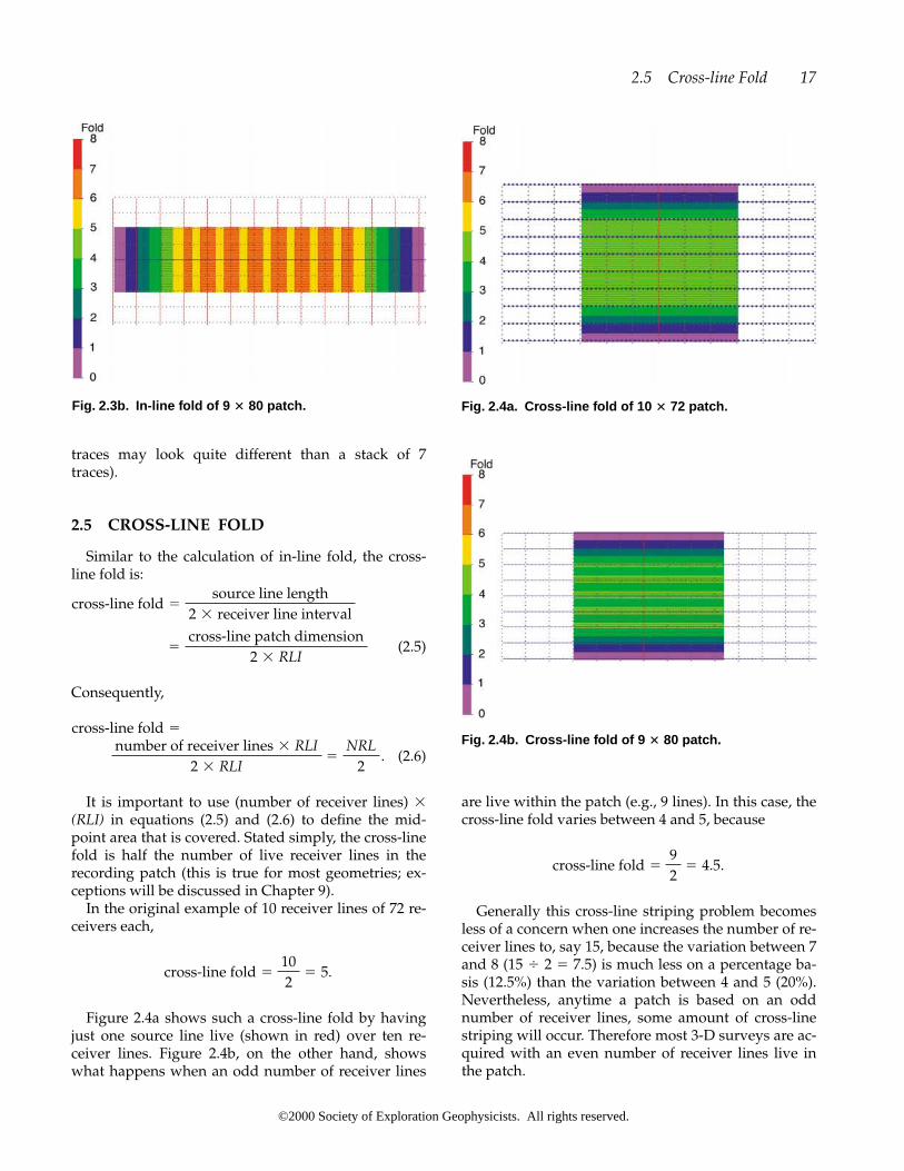
2.5 CROSS-LINE FOLD
Similar to the calculation of in-line fold, the cross-line fold is:
(2.5)
Consequently,
(2.6)
It is important to use (number of receiver lines) �(RLI) in equations (2.5) and (2.6) to define the mid-point area that is covered. Stated simply, the cross-linefold is half the number of live receiver lines in therecording patch (this is true for most geometries; ex-ceptions will be discussed in Chapter 9).
In the original example of 10 receiver lines of 72 re-ceivers each,
Figure 2.4a shows such a cross-line fold by havingjust one source line live (shown in red) over ten re-ceiver lines. Figure 2.4b, on the other hand, showswhat happens when an odd number of receiver lines
cross-line fold �10
2� 5.
number of receiver lines � RLI
2 � RLI�
NRL
2.
cross-line fold �
�cross-line patch dimension
2 � RLI
cross-line fold �source line length
2 � receiver line interval
are live within the patch (e.g., 9 lines). In this case, thecross-line fold varies between 4 and 5, because
Generally this cross-line striping problem becomesless of a concern when one increases the number of re-ceiver lines to, say 15, because the variation between 7and 8 (15 � 2 � 7.5) is much less on a percentage ba-sis (12.5%) than the variation between 4 and 5 (20%).Nevertheless, anytime a patch is based on an oddnumber of receiver lines, some amount of cross-linestriping will occur. Therefore most 3-D surveys are ac-quired with an even number of receiver lines live inthe patch.
cross-line fold �9
2� 4.5.
2.5 Cross-line Fold 17
Fig. 2.3b. In-line fold of 9 � 80 patch. Fig. 2.4a. Cross-line fold of 10 � 72 patch.
Fig. 2.4b. Cross-line fold of 9 � 80 patch.
©2000 Society of Exploration Geophysicists. All rights reserved.

2.6 TOTAL FOLD
The total 3-D nominal fold is the product of in-linefold and cross-line fold:
total nominal fold �
(in-line fold) � (cross-line fold). (2.7)
For the 10 � 72 patch example (Figure 2.5a), totalnominal fold � 6 � 5 � 30. This value is the samevalue initially calculated using the formula:
Fold � SD � NC � B2. (2.8)
However, for the 9 � 80 patch, the in-line foldvaries between 6 and 7 and the cross-line fold changesfrom 4 to 5; hence the total fold varies between 24 and35 (Figure 2.5b). This 3-D fold oscillation is undesir-able and results from lengthening the receiver lines.There were no changes in the source or receiver inter-vals or in the line intervals.
Note: The above equations assume that the bin size re-mains constant and is equal to half of the receiver interval,which in turn is equal to half the source interval. They alsoassume an orthogonal layout with all the source pointswithin the patch.
By choosing the number of live receiver lines to beeven, the cross-line fold is an integer and a smoothcross-line fold distribution results. Noninteger in-lineand cross-line fold introduce striping in the 3-D folddistribution. If the maximum offset for stack exceedsthe offset from any source point to any receiver sta-tion within the patch, then the smoothest fold distrib-utions will result when the in-line and cross-line foldsare integers (Cordsen, 1995b). Careful selection of the
geometric configurations of the live patch is obviouslyone of the more significant components of 3-D design.The principles of design covered to this point can besummarized as
(2.9)
and
(2.10)
These equations can be combined to yield
(2.11)
or
(2.12)
which is
(2.13)
Thus,
(2.14)total fold �patch size
4 � box size.
total fold �patch size
4 � SLI � RLI.
�cross-line patch dimension
2 � RLI,
total fold �in-line patch dimension
2 � SLI
total fold � in-line fold � cross-line fold,
cross-line fold �cross-line patch dimension
2 � RLI.
in-line fold �in-line patch dimension
2 � SLI
18 Planning and Design
Fig. 2.5a. Total fold of 10 � 72 patch.
Fig. 2.5b. Total fold of 9 � 80 patch.
©2000 Society of Exploration Geophysicists. All rights reserved.

This formula holds true for rolling stations andlines on/off (see Chapter 9). Note that of the patchis the area in the subsurface that is covered by mid-points. Hence when rolling the receiver stations andlines, it is the quarter patches of midpoints that over-lap to build up the fold.
Since the ratio of the area of a circle and a squarepatch is R2 � (patch size), the fold within a circle ofradius R [compare equation (2.14)] is
(2.15)
as long as there is continuous coverage of receiversover the entire area and a square patch, which fits out-side of the circle of radius R, is used. This equation es-timates the fold for each horizon (depth) of interest asdefined by that horizon’s mute function (or Xmute).Equation (2.15) estimates the fold for circular patchesas well. It is of note that this equation is totally inde-pendent of the station spacings; those merely definethe natural bin size.
Goodway and Ragan (1995) compared 2-D fold and3-D fold at a particular offset R. For 2-D data the foldis calculated as
(2.16)
The ratio of 3-D and 2-D fold at offset R can then bedefined as
(2.17)
This fold ratio is linear with offset R. Large linespacings (coarse sampling) lead to a low fold ratio,which might be acceptable for deeper targets (withthe large increase in fold at far offsets). Decreasing theline spacings increases the fold ratio, therefore in-creasing fold at near offset, which is good for shallowtargets. A compromise could be accomplished by us-ing a narrow azimuth patch (see Section 3.3) to evenout the fold distribution.
2.7 FOLD TAPER
Another important factor to consider when calcu-lating fold is the fold taper. This parameter describesthe area around the full-fold area where the fold
R � 2-D source interval
4 � SLI � RLI.
Fold RatioR (3-D/2-D) �
2-D foldR �offset R
source interval.
foldR �R2
4 � SLI � RLI�
R2
4 � box size,
1�4
build-up occurs. The width of this strip is not neces-sarily the same in the in-line and cross-line directionsand needs to be calculated separately as follows:
(2.18)
and
(2.19)
By substituting the formulas for in-line and cross-line fold, one can derive the following useful form ofthese equations:
(2.20)
(2.21)
Rule of Thumb: The fold taper is approximately equal toone quarter of the patch dimension in the fold-taper direc-tion.
These equations define fold taper in units of meters(or feet). A better way to express fold taper is in termsof source and receiver line intervals because that defi-nition makes it easier to study the effects of fold taperwhen looking at fold maps. Hence the term “foldrate” is defined as the increase in fold per line intervalin a specified direction, or
(2.22)
and
(2.23)
In the example of the 10 � 72 patch, the tapers andfold rates are as follows:
cross-line taper � � 5
2 0.5� � 360 m � 720 m
in-line taper � � 6
2 0.5� � 360 m � 900 m
cross-line fold rate �total fold � RLI
cross-line fold taper.
in-line fold rate �total fold � SLI
in-line fold taper,
cross-line taper �cross-line patch size
4
RLI
2
in-line taper �in-line patch size
4
SLI
2
� � cross-line fold
2 0.5� � RLI.
cross-line taper
in-line taper � � in-line fold
2 0.5� � SLI,
2.7 Fold Taper 19
©2000 Society of Exploration Geophysicists. All rights reserved.

and
which equals 2 source line interval of fold taper, and
which equals 2 receiver line intervals.
2.8 SIGNAL-TO-NOISE RATIO (S/N)
For square bins, the S/N is directly proportional to the length of one side of the bin (Figure 2.6). Therefore, only a slight change in the selection of the bin size can have a major effect on the fold and the S/N. The designer of a 3-D survey needs to begiven clear and precise specifications for these parameters to effectively optimize the 3-D design. If the fold drops below the required level for only a few bins, that does not necessarily mean that the 3-D survey is poorly designed. Increasing the fold by only a small percentage on an otherwise well-designed survey may cost an unreasonable amount of money to satisfy the fold requirements of a fewbins.
� 15 fold per RLI,
cross-line fold rate �30 fold � 360 m
720 m
1�2
� 12 fold per SLI,
in-line fold rate �30 fold � 360 m
900 m
2.9 BIN SIZE
It is important to differentiate between the bin sizeand the bin interval. The bin size is the area overwhich the traces are stacked. The bin interval deter-mines how far apart these trace summations are dis-played. Most of the time bin dimension and bin inter-val are used interchangeably (as they are in this text),because they have the same value, but occasionallythey may differ (e.g. flex-binning in marine surveys).
The selection of bin size and fold go hand in hand.The fold is a quadratic function of the length of oneside of the bin (Figure 2.7). The basic fold equation de-rived in Section 2.3 indicates that the constant relatingfold to (bin size)2 is the midpoint density (i.e., thenumber of midpoints per square unit area), or
fold � SD � NC � B2. (2.24)
The preferred shape of a 3-D data bin is a square.Rectangular bins may be acceptable to highlight cer-tain geological features if the lateral resolution neededin one direction is different from the required resolu-tion in the other direction. Also, the spatial samplingrequirements for migration might be different in dif-ferent directions. Sometimes cost issues will deter-mine a different receiver station than source point in-terval; hence, natural bin sizes may differ. In somecases, rectangular bins may create problems becausethe smaller number of subsurface measurements inthe long direction of the bins limits the resolvingpower of geological features in that direction.
20 Planning and Design
Fig. 2.6. Signal-to-noise ratio (S/N) versus bin size. Fig. 2.7. Fold versus bin size.
©2000 Society of Exploration Geophysicists. All rights reserved.

Bin size can be determined by examining three fac-tors: target size, maximum unaliased frequency dueto dip, and lateral resolution, and then picking thesmallest value of bin size provided by these analysesas the design parameter.
2.9.1 Target Size
Normally two to three traces, positioned so theypass through a small target, will allow that target tobe seen in a 3-D image, because this means four tonine traces will be related to the target on a time sliceof the horizon of interest. For example, if the target isa small reef or a narrow channel sand then the binsshould be small enough to get at least two (preferablythree) traces across the target. This imaging require-ment gives a 3-D designer an initial (and generally toolarge) estimate for a bin size, which is
(2.25)
Consider the following example where a 3-D sur-vey in Alberta crossed a 300-m ( mi) wide channel(Cordsen, 1993b), which had been difficult to definewith 2-D data. Within this narrow channel, a 100-m ( mi) wide sand anomaly surrounded by shale couldbe identified on the 3-D data (Figure 2.8). The choiceof 24 m � 24 m (78 ft � 78 ft) bin size allowed thesand anomaly to be recognized on four traces crossingthe channel. This 4-trace response is close to the mini-mum that is required for target recognition by manyinterpreters. Had the bin size been chosen muchlarger, the sand anomaly may not have shown up atall.
116
15
Bin size �target size
3.
2.9 Bin Size 21
Fig. 2.8. Bin size and target size.
The power of 3-D data is that an interpreter can re-late anomalies from one cross-line to the next cross-line and follow the seismic expression continuously.Older 2-D data would not have convinced manage-ment to drill this narrow sand body, but several suc-cessful oil wells have been drilled into this channelbased on the 3-D data.
2.9.2 Maximum Unaliased Frequency
Each dipping seismic reflection event has a maxi-mum possible unaliased frequency f before migrationthat depends on the velocity to the target, the value ofthe geological dip �, and the bin size B. Referring toFigure 2.9a, these parameters are related as
(2.26)
One needs to take account of the fact that �t repre-sents only wavelength since two-way traveltime ismeasured and two samples per wavelength are re-quired to avoid aliasing. Thus
(2.27)
and replacing �t
(2.28)
Therefore,
(2.29)
and
(2.30)
The reflector dip � is very important in these twoequations. A negligible dip produces very large val-ues for the largest bin size, which does not causealiasing, and for maximum unaliased frequency. Thelargest dip of 90° puts the most constraint on thesecalculations. The main question is to decide which ve-locities or frequencies should be used for the bin sizecalculations. Common practice has been to use the av-erage velocity Vave and the dominant frequency fdom
B �V
4 � f � sin �.
f �V
4 � B � sin �
sin � �V
4 � B � f.
�t ��
4 � V�
1
4 � f,
14
sin � �V � �t
B.
©2000 Society of Exploration Geophysicists. All rights reserved.

for a constant-velocity earth (as in Figures 2.9a and2.9b), giving
(2.31)fdom �Vave
4 � B � sin �.
For example:
or
Solving for the bin size B,
(2.32)
yields bin size values of (if fdom � 60 Hz):
or
Most geological scenarios do not warrant the con-stant-velocity medium assumption. A velocity that in-creases linearly with depth is a better assumption inmany basins. A common velocity function is
Vz � V0 kZ, (2.33)
where Vz is the depth-varying velocity, V0 is the veloc-ity at surface, k is a constant (usually >0), and Z isdepth. Margrave (1997) used this depth-varying ve-locity to determine the bin size.
One needs to consider ray-bending to avoid over-constraining the bin size (see Bee et al., 1994). An ex-ample of ray-bending is illustrated in Figure 2.9c (af-ter Liner and Gobeli, 1997). The raypaths are parallelfor ray parameter p until the up-dip raypath reachesthe reflector. The ray parameter p is a constant that isindependent of depth and is defined as
(2.34)
where �0 is the take-off angle for the ray rather thanthe geological dip. The bin size for a depth varyingvelocity model can be calculated as follows:
(2.35)B �Vz
4 � fmax � sin �.
p �sin �0
Vz
,
B �7500 ft/s
4 � 60 Hz � sin 15�� 121 ft.
B �2500 m/s
4 � 60 Hz � sin 15�� 40 m,
B �Vave
4 � fdom � sin �,
fdom �7500 ft/s
4 � 82.5 ft � sin 15�� 88 Hz.
fdom �2500 m/s
4 � 25 m � sin 15�� 97 Hz
22 Planning and Design
Fig. 2.9. Bin size B and maximum unaliased frequency;a. before migration, b. after migration, c. linear-velocityearth.
©2000 Society of Exploration Geophysicists. All rights reserved.

The interval velocity Vint immediately above thehorizon [or Vz in equation (2.35)], rather than the av-erage velocity, should be used for calculations of binsize at the target. This choice of bin size assures thatthe maximum frequency at the target fmax is notaliased with reflector dip �. Therefore,
(2.36)
For example:
or
Solving for the bin size B,
(2.37)
For example if fmax � 80 Hz, then
or
Any frequencies at the zone of interest that arehigher than fmax will be aliased before migration. Inother words, the true dip of the event will be con-tained only in frequencies lower than this value. Forthe following discussions, the maximum frequencyand the interval velocity at the target are used.
The above equations are based on recording twosamples per wavelength of the maximum frequency.Many companies use more stringent requirements ofthree or four (or even noninteger values such as 2.8)samples per wavelength of the dominant frequency,which greatly reduces the bin size and increases thesurvey cost.
Note that the process of migration lowers frequen-cies on all dipping events; the rule being that thesteeper the dip, the lower the frequencies after migra-tion. Any aliasing of frequencies prior to migration
bin size B �10 000 ft/s
4 � 80 Hz � sin 15�� 120 f t.
bin size B �3000 m/s
4 � 80 Hz � sin 15�� 36 m
B �Vint
4 � fmax � sin �.
fmax �10 000 f t/s
4 � 82.5 f t � sin 15�� 118 Hz.
fmax �3000 m/s
4 � 25 m � sin 15�� 116 Hz
fmax �Vint
4 � B � sin �.
may look like frequency dispersion after migrationdue to the particular migration algorithm that is used.The correct choice of bin size successfully preservesthe desired maximum frequency through the migra-tion step. The connection between bin size B and fmax
after migration is given by similar formulas as abovein which sin � is replaced by tan � (Figure 2.9b).
Metric Example:
Using the formula, calculate
fmax for the following three sets of numbers (Vint �
3000 m/s):
fmax �Vint
4 � B � sin �,
2.9 Bin Size 23
Using the formula, calculate
the bin size B for the following three sets of numbers(Vint � 3000 m/s):
B �Vint
4 � fmax � sin �,
Imperial Example:
Using the formula, calculate
fmax for the following three sets of numbers (Vint �
10 000 ft/s):
fmax �Vint
4 � B � sin �,
Using the formula, calculate the
bin size B for the following three sets of numbers (Vint �
10 000 ft/s):
B �Vint
4 � fmax � sin �,
Dip (in degrees) B (meters) fmax (Hz)
5 10020 2535 15
Dip (in degrees) B ( ft) fmax (Hz)
5 44020 11045 55
Dip (in degrees) fmax (Hz) B( ft)
15 8020 6030 40
Dip (in degrees) fmax (Hz) B (meters)
15 10025 6040 40
©2000 Society of Exploration Geophysicists. All rights reserved.

Such aliasing frequency tables could easily be devel-oped for other interval velocities Vint relative to thearea of interest.
2.9.3 Lateral Resolution
Before migration, two diffractions are not resolvedif they are closer than the first Fresnel zone diameter.This diameter is usually a large value (500 m or more)and means that on the CMP stack, small, closelyspaced faults can be missed. After migration, the lat-eral resolution depends on the maximum frequencythat is reflected from the zone of interest. In the pastseveral years, different definitions and formulas forlateral resolution have been published.
Denham (1980):
where � is the maximum ray angle contributing to themigration, RH is horizontal resolution, and RV is verti-cal resolution.
Claerbout (1985):
“Resolving power is customarily defined as about halfthe effective wavelength. . . .”
Embree (1985):
Freeland and Hogg (1990):
RL � RV �V
2B,
dXr �0.3 � V
fmax � sin �.
RH �RV
sin �,
24 Planning and Design
Table 2.2. Calculation of fmax.
Dip (degrees) Subsurface trace spacing in meters
10 15 20 25 30 50 100
5 861 574 430 344 287 17210 432 288 216 173 144 86 4315 290 193 145 116 97 58 2920 219 146 110 73 44 2225 177 118 89 71 59 35 1830 150 100 75 60 50 30 1535 131 65 52 44 26 1340 117 78 58 47 39 23 1245 106 71 53 42 35 21 11 in Hz
87
88
86
f max �Vint
4 � bin size � sin �
Table 2.3. Calculation of bin size B.
Dip (degrees) fmax in Hz
40 50 60 70 80 90 100
5 215 172 143 123 108 96 8610 108 86 72 62 54 48 4315 72 58 48 41 36 3220 55 44 37 31 27 24 2225 44 35 25 22 20 1830 38 30 25 21 19 17 1535 33 26 22 19 16 15 1340 23 19 17 15 13 1245 27 21 18 15 13 12 11 in meters
29
30
29
B �Vint
4 � fmax � sin �
Alias Frequency TablesVint � 3000 m/s
Table 2.4. Calculation of fmax.
Dip (degrees) Subsurface trace spacing in feet
41 55 82.5 110 165 220 440
5 700 522 348 261 174 13010 351 262 175 131 87 65 3315 236 176 117 88 59 44 2220 178 133 89 44 33 1725 144 108 72 54 36 27 1330 122 91 61 45 30 23 1135 106 79 53 40 26 20 1040 95 71 47 35 24 18 945 86 43 32 21 16 8 in Hz64
66
65
fmax �Vint
4 � B � sin �
Alias Frequency TablesVint � 10 000 ft/s
Table 2.5. Calculation of bin size B.
fmax in Hz
Dip (degrees) 40 50 60 70 80 90 100
5 717 574 478 410 359 319 28710 360 288 240 206 180 160 14415 241 193 161 138 107 9720 183 146 104 91 81 7325 148 118 99 85 74 66 5930 100 83 71 63 56 5035 109 87 73 62 54 48 4440 97 78 65 56 49 43 3945 88 71 59 51 44 39 35 in feet
125
122121
B �Vint
4 � fmax � sin �
©2000 Society of Exploration Geophysicists. All rights reserved.

where RL � lateral resolution, RV � vertical resolu-tion, and B � bandwidth. This equation assumes timeperiod � half bandwidth.
Ebrom et al. (1995):
where
is half the line length, and Z is the target depth.
Vermeer (1997):
Vermeer interprets this as where Vmin is the
minimum apparent velocity of the P-wave data and�x, max is the scattering angle and not reflector dip.
Finite recording apertures (patches) in space andtime imprint a strong spatial-temporal variation onthe spectral content of the migrated section (Mar-grave, 1997). Not everyone agrees on the definition ofresolution: Is it one half the dominant wavelength(Claerbout, 1985; Freeland and Hogg, 1990), or is itone quarter of the minimum wavelength (Ebrom, etal., 1995; Vermeer, 1997), or somewhere in between(Embree, 1985)? One of the key questions regardingresolution is the ability of the interpreter to recognizethe feature being resolved. This ability is interpreter-dependent and should be considered when pickingthe bin size.
In 3-D surveys, the migration aperture variesthroughout the survey because of edge effects. It istherefore reasonable to use a migration aperture anglesuch as 30° in Vermeer’s formula. It is also reasonableto expect the resolution to change by a factor of 2 ormore from the edges of the survey to the center. Theexistence of noise (ground roll, multiples, etc.) causesfurther loss of resolution to a limit that is commonlytermed “achievable resolution.” In practice, the “ac-tual resolution” will be less than the “achievable reso-lution” because of errors in processing such as usingthe wrong velocity model, suboptimal phase compen-sation, etc.
For the purposes of the present discussion, it is as-sumed that lateral resolution will be between one-quarter and one-half the dominant wavelength. Thedominant frequency can be measured directly from
Vmin
4 � fmax
,
Rx �V
4 � fmax � sin �x, max
.
L
2
�min �1
fmax
, � � arctan L
2�,
RL ��min
4 � sin �,
the seismic section, thus a simple guideline equationfor bin size is:
(2.38)
where N varies from 2 to 4. Suppose the dominant frequency fdom at the selected target is 50 Hz. If the in-terval velocity immediately above this target is 3000m/s (10 000 ft/s), then the spatial wavelength,
or
and the bin size is:
or
Using the examples of the last few pages, the lateralresolution defines the range of possible bin sizes from aminimum of 15 m (50 ft) to a maximum acceptable binsize of 30 m (100 ft) (Table 2.6). There is little point inchoosing a bin size less than that needed for lateral res-olution. Smaller bins would provide no additional in-formation. Correspondingly, with larger bins there is adanger that some events will not be resolved laterally.
A bin size less than one quarter of the dominantwavelength results in over-sampling and provides noadditional information. A bin size greater than half ofthe dominant wavelength results in spatial aliasingand missing information.
bin size B �10 000 f t/s
2 � 50 Hz� 100 ft (or 50 f t for N � 4).
bin size B �3000 m/s
2 � 50 Hz� 30 m (or 15 m for N � 4),
� 10 000 f t/s
50 Hz� 200 f t�,�dom is
3000 m/s
50 Hz� 60 m
Bin Size B �Vint
N � fdom
,
2.9 Bin Size 25
Table 2.6. Selection of bin size.
Parameter Bin Size
Target Size 33 m (100 ft)
Maximum Unaliased Frequency 36 m (120 ft)Lateral Resolution 15–30 m (50–100 ft)
A bin size of 30 m is selected for this example.
2.9.3.1 Lateral Resolution after Migration
The lateral resolution that exists after migration can be explained using Figure 2.10. Four events areshown in f-k space both before and after migration.The effect of migration is to map high frequencies to low frequencies at the same wavenumber. The
©2000 Society of Exploration Geophysicists. All rights reserved.
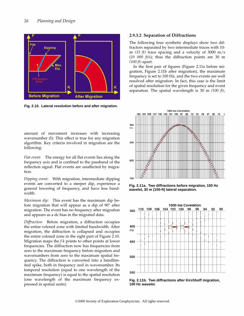
amount of movement increases with increasingwavenumber (k). This effect is true for any migrationalgorithm. Key criteria involved in migration are thefollowing:
Flat event: The energy for all flat events lies along thefrequency axis and is confined to the passband of thereflection signal. Flat events are unaffected by migra-tion.
Dipping event: With migration, intermediate dippingevents are converted to a steeper dip, experience ageneral lowering of frequency, and have less band-width.
Maximum dip: This event has the maximum dip be-fore migration that will appear as a dip of 90° aftermigration. The event has no frequency after migrationand appears as a dc bias in the migrated data.
Diffraction: Before migration, a diffraction occupiesthe entire colored zone with limited bandwidth. Aftermigration, the diffraction is collapsed and occupiesthe entire colored zone in the right part of Figure 2.10.Migration maps the f-k points to other points at lowerfrequencies. The diffraction now has frequencies fromzero to the maximum frequency before migration andwavenumbers from zero to the maximum spatial fre-quency. The diffraction is converted into a bandlim-ited spike, both in frequency and in wavenumber. Itstemporal resolution (equal to one wavelength of themaximum frequency) is equal to the spatial resolution(one wavelength of the maximum frequency ex-pressed in spatial units).
2.9.3.2 Separation of Diffractions
The following four synthetic displays show two dif-fractors separated by two intermediate traces with 10-m (33 ft) trace spacing and a velocity of 3000 m/s (10 000 ft/s); thus the diffraction points are 30 m (100 ft) apart.
In the first pair of figures (Figure 2.11a before mi-gration, Figure 2.11b after migration), the maximumfrequency is set to 100 Hz, and the two events are wellresolved after migration. In fact, this case is the limitof spatial resolution for the given frequency and eventseparation. The spatial wavelength is 30 m (100 ft),
26 Planning and Design
Fig. 2.10. Lateral resolution before and after migration.
Fig. 2.11a. Two diffractions before migration, 100 Hzwavelet, 30 m (100-ft) lateral separation.
Fig. 2.11b. Two diffractions after Kirchhoff migration,100 Hz wavelet.
©2000 Society of Exploration Geophysicists. All rights reserved.

which is borne out by the facts that each diffractor af-ter migration is on a peak and that there are twotraces (with troughs) between the events. Wavelengthvalues can be calculated using
Vint � fmax � �max, (2.39)
or
(2.40)
or
(2.41)
where Vint is the velocity immediately above target,fmax is maximum frequency, fdom is the dominant fre-quency � fmax, �max is the wavelength at fmax, and�dom is the wavelength at fdom.
In this example:
spatial wavelength �
or
spatial wavelength �
The spatial resolution is also 30 m (100 ft), i.e., onewavelength of the maximum frequency, or one-half-wavelength of the dominant frequency. In this casethe maximum frequency was used in the calculation.One can get the same answer by using the half-wave-length of the dominant frequency of 50 Hz.
The second pair of figures (Figure 2.12a before mi-gration, Figure 2.12b after migration) shows the effectof reducing the maximum model frequency to 50 Hz,which corresponds to a spatial wavelength of 60 m(200 ft). In this case, both diffractors are on the samepositive amplitude “spatial wavelet” and the lateralresolution is lost.
Spatial wavelength �
or
Spatial wavelength �10 000 ft/s
50 Hz� 200 f t.
3000 m/s
50 Hz� 60 m
10 000 ft/s
100 Hz� 100 f t.
3000 m/s
100 Hz� 30 m
12
�dom �Vint
fdom
� 2�max,
�max �Vint
fmax
,
2.9.4 Vertical Resolution
A classic paper on vertical (temporal) resolution hasbeen published by Kallweit and Wood (1982). Theydiscuss various criteria (Rayleigh, Ricker, and Widess)and how their criteria can be used to describe thewidth of a wavelet as a measure of temporal resolu-tion. In Vermeer (1999a), it is pointed out that the con-figuration of 3-D sources and receivers leads to a sig-nificant difference between vertical and lateralresolution. Vermeer suggests the following formula asa more practical alternative to the more optimistic for-mula derived from zero-offset considerations andWidess criteria (Rz � 1/4 fmax),
Rz � cV/(2 fmax cos i), (2.42)
2.9 Bin Size 27
Fig. 2.12a. Two diffractions before migration, 50 Hz,30 m (100-ft) lateral separation.
Fig. 2.12b. Two diffractions after Kirchhoff migration,50 Hz wavelet.
©2000 Society of Exploration Geophysicists. All rights reserved.

where Rz is the vertical resolution in spatial units, c isa constant depending on the criterion used (Rayleigh,etc.), V is the local interval velocity over the physicaldimension of a temporal wavelet, fmax is the maximumfrequency recorded from the target, and cos i is the co-sine of angle i that is the half-angle subtended be-tween source and receiver to a point at depth; cos ican be interpreted as the NMO stretch which reducesfmax to fmax � cos i.
Example:
V � 2500 m/s,
c � 0.715 (Rayleigh criterion),
cos i � 0.9, fmax � 40 HZ.
Then
Rz � 0.715 � 2500/2 � 40 � 0.9 � 25 m.
In most cases, it is best to use c � 0.715. In somecases, it may be possible to use c � 0.25 (1/4 wave-length criterion) if all parameters around a targethorizon are more or less constant except for thick-ness. In such a case, tuning effects can be used withconfidence. The value of cos i can also be set to 0.9,which corresponds approximately to the “maximumoffset equals depth criterion” for muting (NMOstretch).
Thus a practical equation is
Rz � 0.715 V/(2 fmax 0.9) � 0.4 V/fmax. (2.43)
This equation states that the vertical resolution Rz isof the wavelength of the maximum frequency re-
flecting from the target to be resolved.
Let’s Design a 3-D—Part 1
For the following exercise a simple approximationfor calculating the sine can be used, which is
For example:
sin 6° � 0.1
sin 12° � 0.2
sin 18° � 0.3
sin (dip) �dip
60.
25
This approximation holds true within 6% for angles�45°.
In this example, these are the following known para-meters (metric):
existing 2-D data of goodquality have 30 fold
steepest dips 20°shallow markers needed for
isochroning have 500 m offsetstarget depth 2000 mtarget two-way time 1.5 sbasement depth 3000 mVint immediately above the
target horizon 4200 m/sfdom at the target horizon 50 Hzfmax at the target horizon 70 Hzlateral target size 300 m
Orthogonal design method should be used.
Desired fold:
up to full 2-D fold �
Bin size:
a) for target size: B � target size � 3 �
b) for alias frequency: B � Vint � (4 � fmax � sin �) �
c) for lateral resolution: B � Vint � (N � fdom), (N � 2 to 4) � ____ to _____bin size B �
RI �
SI �
Let’s Design a 3-D—Part 1 (Imperial)
In this example, these are the following known parameters:
existing 2-D data of good quality have 30 foldsteepest dips 20°shallow markers needed for isochroning
have 1500 ft offsetstarget depth 6000 fttarget two-way time 1.5 sbasement depth 10 000 ftVint immediately above the target horizon 14 000 ft/sfdom at the target horizon 50 Hzfmax at the target horizon 70 Hzlateral target size 1000 ft
Orthogonal design method should be used.
12
28 Planning and Design
©2000 Society of Exploration Geophysicists. All rights reserved.

Desired fold: up to full 2-D fold �
Bin size:
a) for target size: B � target size � 3 �
b) for alias frequency: B � Vint � (4 � fmax � sin �) �
c) for lateral resolution: B � Vint� (N � fdom ), (N �
2 to 4) � ____ to _____bin size B �
RI �
SI �
2.10 XMIN
The bin at the center of the box formed by two adja-cent receiver lines and two source adjacent lines hasthe largest minimum offset of any bin within the box.The largest minimum offset therefore is the diagonalof this box (Figure 2.13a). The source and receiver lineintervals (SLI and RLI) are largely determined by therequired value for Xmin. In orthogonal, brick, and zig-zag designs (see Chapter 5), the largest minimum off-set is related directly to SLI and RLI. For orthogonalsurveys, Xmin is determined by:
Xmin � (RLI2 SLI 2)1/2. (2.44)
12
Obviously, the larger of RLI and SLI has the greaterinfluence on Xmin. Therefore, in an orthogonal design,a square box is the ideal case for minimizing Xmin.
Going back to the practice example:
Xmin � (3602 3602)1/2 m � 509 m
or
Xmin � (13202 13202)1/2 ft � 1867 ft.
Generally lines are offset from their coincident posi-tions by one bin size at their intersection points (Fig-ure 2.13b) in order to reduce duplicate raypaths. Theformula for Xmin changes slightly for this geometry asfollows:
Xmin � [(RLI 0.5 � SI)2
(SLI 0.5 � RI)2]1/2. (2.45)
When offsetting the source or receiver lines in thisway, the four bins in the center of the box have thesame Xmin, rather than just the center bin having thelargest Xmin. Going back to the practice example:
Xmin � [(360 – 30)2 (360 – 30)2]1/2 m � 467 m
or
Xmin � [(1320 – 55)2 (1320 – 55)2]1/2 ft � 1789 ft.
2.10 XMIN 29
Fig. 2.13a. Xmin definition with coincident source and re-ceiver stations at corners of box.
Fig. 2.13b. Xmin definition with half-station line shifts atbox corners.
©2000 Society of Exploration Geophysicists. All rights reserved.
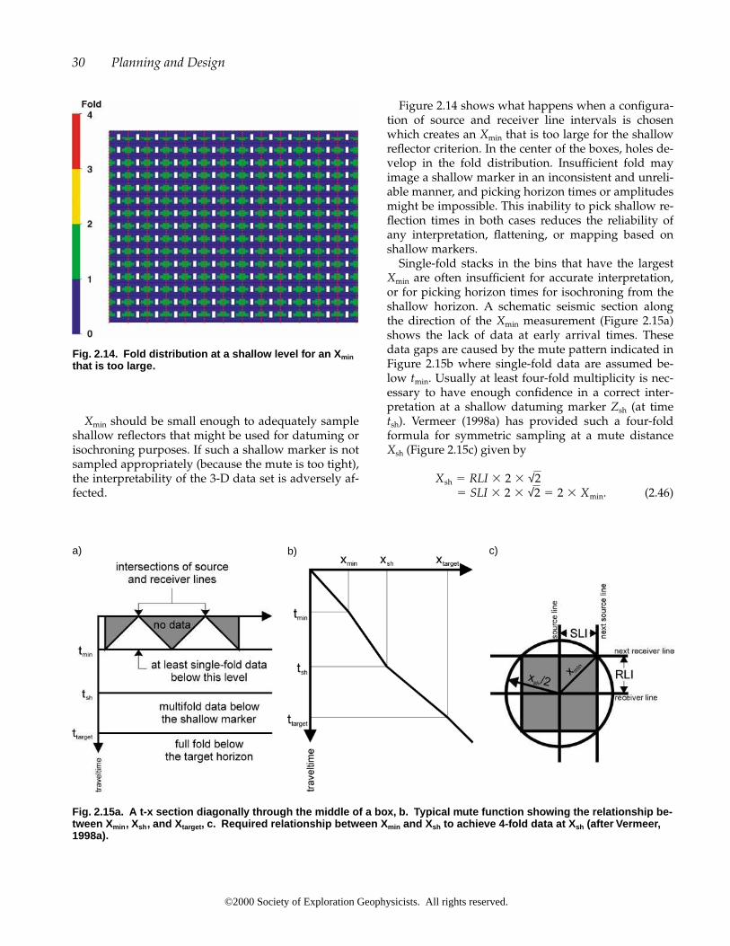
Xmin should be small enough to adequately sampleshallow reflectors that might be used for datuming orisochroning purposes. If such a shallow marker is notsampled appropriately (because the mute is too tight),the interpretability of the 3-D data set is adversely af-fected.
Figure 2.14 shows what happens when a configura-tion of source and receiver line intervals is chosenwhich creates an Xmin that is too large for the shallowreflector criterion. In the center of the boxes, holes de-velop in the fold distribution. Insufficient fold mayimage a shallow marker in an inconsistent and unreli-able manner, and picking horizon times or amplitudesmight be impossible. This inability to pick shallow re-flection times in both cases reduces the reliability ofany interpretation, flattening, or mapping based onshallow markers.
Single-fold stacks in the bins that have the largestXmin are often insufficient for accurate interpretation,or for picking horizon times for isochroning from theshallow horizon. A schematic seismic section alongthe direction of the Xmin measurement (Figure 2.15a)shows the lack of data at early arrival times. Thesedata gaps are caused by the mute pattern indicated inFigure 2.15b where single-fold data are assumed be-low tmin. Usually at least four-fold multiplicity is nec-essary to have enough confidence in a correct inter-pretation at a shallow datuming marker Zsh (at timetsh). Vermeer (1998a) has provided such a four-foldformula for symmetric sampling at a mute distanceXsh (Figure 2.15c) given by
(2.46)� SLI � 2 � √2 � 2 � Xmin.Xsh � RLI � 2 � √2
30 Planning and Design
Fig. 2.14. Fold distribution at a shallow level for an Xminthat is too large.
Fig. 2.15a. A t-x section diagonally through the middle of a box, b. Typical mute function showing the relationship be-tween Xmin , Xsh , and Xtarget , c. Required relationship between Xmin and Xsh to achieve 4-fold data at Xsh (after Vermeer,1998a).
a) b) c)
©2000 Society of Exploration Geophysicists. All rights reserved.
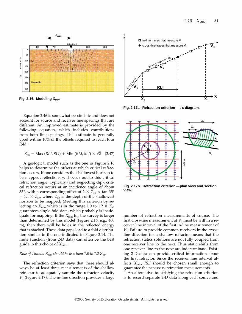
number of refraction measurements of course. Thefirst cross-line measurement of V1 must be within a re-ceiver line interval of the first in-line measurement ofV1. Failure to provide common receivers in the cross-line direction for a shallow refractor means that therefraction statics solutions are not fully coupled fromone receiver line to the next. Thus static shifts fromone receiver line to the next are indeterminate. Exist-ing 2-D data can provide critical information aboutthe first refractor. Since the receiver line interval af-fects Xmin, RLI should be chosen small enough toguarantee the necessary refraction measurements.
An alternative to satisfying the refraction criterionis to record separate 2-D data along each source and
2.10 XMIN 31
Fig. 2.16. Modeling Xmin .
Fig. 2.17a. Refraction criterion — t-x diagram.
Equation 2.46 is somewhat pessimistic and does notaccount for source and receiver line spacings that aredifferent. An improved estimate is provided by thefollowing equation, which includes contributionsfrom both line spacings. This estimate is generallygood within 10% of the offsets required to reach fourfold.
(2.47)
A geological model such as the one in Figure 2.16helps to determine the offsets at which critical refrac-tion occurs. If one considers the shallowest horizon tobe mapped, reflections will occur out to this criticalrefraction angle. Typically (and neglecting dip), criti-cal refraction occurs at an incidence angle of about35°, with a corresponding offset of 2 � Zsh � tan 35°� 1.4 � Zsh, where Zsh is the depth of the shallowesthorizon to be mapped. Meeting this criterion by se-lecting an Xmin which is in the range 1.0 to 1.2 � Zsh
guarantees single-fold data, which probably is inade-quate for mapping. If the Xmin for the survey is largerthan determined by this model (Figure 2.16; e.g., 400m), then there will be holes in the reflected energythat is stacked. These data gaps lead to a fold distribu-tion similar to the one indicated in Figure 2.14. Themute function (from 2-D data) can often be the bestguide to this choice of Xmin.
Rule of Thumb: Xmin should be less than 1.0 to 1.2 Zsh.
The refraction criterion says that there should al-ways be at least three measurements of the shallowrefractor to adequately sample the refractor velocityV1 (Figure 2.17). The in-line direction provides a large
Xsh � Max (RLI, SLI) Min (RLI, SLI) � √2
Fig. 2.17b. Refraction criterion —plan view and sectionview.
©2000 Society of Exploration Geophysicists. All rights reserved.

receiver line. This will completely determine sourceand receiver delays (statics) and near-surface veloci-ties. The cost of a separate 2-D refraction statics sur-vey may well be justified for 3-D surveys with widelyspaced source and receiver lines rather than reducingthe line intervals.
2.11 XMAX
The required maximum offset depends on thedepth to the deeper targets that must be imaged. Onealso needs to take into account normal moveout(NMO) assumptions and dip. It is strongly suggestedthat the designer pay particular attention to the offsetdistribution on a line-by-line basis.
The processing mute of the far offsets has a greatimpact on selection of the maximum recorded offset(Cordsen, 1995b). If Xmax in the patch is measured asthe maximum in-line offset (Figure 2.18a), then traceson receiver lines farther away from the source pointare muted. The fold value is limited by Xmute. Sincethe ratio of the area of a circle and a square patch isR2 � (patch size), the fold within a circle of radius Rreduces to (compare section 2.6)
(2.48)
R is equal to Xmute. If, however, Xmax is measuredalong the diagonal of the patch, then no traces will bemuted and Xmax is indeed the maximum offset in thesurvey. In this case, all traces will be used in the stack(Figure 2.18b). This geometry makes fold calculationseasier, and a more uniform fold distribution can be ac-complished (see Sections 2.4, 2.5, and 2.6). Other as-pects of patch design are discussed in Section 3.4.When Xmax is measured in-line, the area of the patch isexactly twice the area of the patch with Xmax mea-sured diagonally.
The recorded Xmax can be changed by placingsource points off-center in the receiver patch. In thisapproach, the number of far offsets that exceed the“shorter far offsets” are reduced, which may not pro-vide an adequate far-offset contribution.
In typical 3-D receiver patches, the mix of offsets isnonlinear, i.e., there are few near offsets and many faroffsets (Figure 2.19). In fact, wide azimuth surveyshave offset distributions that are linear in offsetsquared (see Section 3.3). Narrow azimuth surveystend to have more linear offset distributions, with theoffset distribution of a 2-D line being the end member.The dotted line in Figure 2.19 is the distribution for a
Fold �(SD � NC � B2) � R2
Patch Size.
wide azimuth orthogonal design with eight receiverlines in the patch.
A good approximation (for a wide azimuth patch)is that the first 33% of the offset range includes 7% of
32 Planning and Design
Fig. 2.18a. In-line Xmax.
Fig. 2.18b. Diagonal Xmax.
©2000 Society of Exploration Geophysicists. All rights reserved.
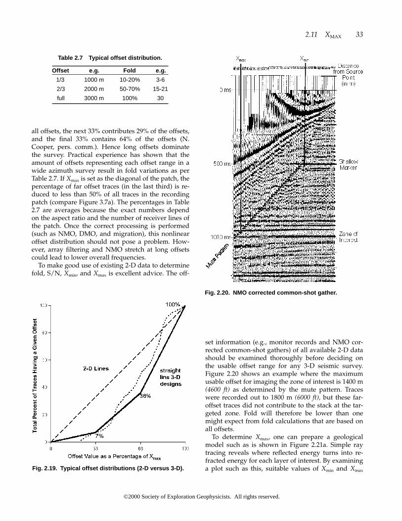
all offsets, the next 33% contributes 29% of the offsets,and the final 33% contains 64% of the offsets (N.Cooper, pers. comm.). Hence long offsets dominatethe survey. Practical experience has shown that theamount of offsets representing each offset range in awide azimuth survey result in fold variations as perTable 2.7. If Xmax is set as the diagonal of the patch, thepercentage of far offset traces (in the last third) is re-duced to less than 50% of all traces in the recordingpatch (compare Figure 3.7a). The percentages in Table2.7 are averages because the exact numbers dependon the aspect ratio and the number of receiver lines ofthe patch. Once the correct processing is performed(such as NMO, DMO, and migration), this nonlinearoffset distribution should not pose a problem. How-ever, array filtering and NMO stretch at long offsetscould lead to lower overall frequencies.
To make good use of existing 2-D data to determinefold, S/N, Xmin, and Xmax is excellent advice. The off-
set information (e.g., monitor records and NMO cor-rected common-shot gathers) of all available 2-D datashould be examined thoroughly before deciding onthe usable offset range for any 3-D seismic survey.Figure 2.20 shows an example where the maximumusable offset for imaging the zone of interest is 1400 m(4600 ft) as determined by the mute pattern. Traceswere recorded out to 1800 m (6000 ft), but these far-offset traces did not contribute to the stack at the tar-geted zone. Fold will therefore be lower than onemight expect from fold calculations that are based onall offsets.
To determine Xmax, one can prepare a geologicalmodel such as is shown in Figure 2.21a. Simple raytracing reveals where reflected energy turns into re-fracted energy for each layer of interest. By examininga plot such as this, suitable values of Xmin and Xmax
2.11 XMAX 33
Fig. 2.19. Typical offset distributions (2-D versus 3-D).
Fig. 2.20. NMO corrected common-shot gather.
Table 2.7 Typical offset distribution.
Offset e.g. Fold e.g.
1/3 1000 m 10-20% 3-6
2/3 2000 m 50-70% 15-21
full 3000 m 100% 30
©2000 Society of Exploration Geophysicists. All rights reserved.

can be determined for each event and hence for theentire model.
2.11.1 Target Depth
The largest offsets that should be recorded are gen-erally the same magnitude as the target depth. Manymodels and survey data have shown this to be a goodfirst approximation.
Rule of Thumb: Xmax should be approximately the sameas the primary target depth, usually expressed as Xmax �
Target Depth.
2.11.2 Direct Wave Interference
The direct wave, which travels from source to re-ceiver by the shortest distance, will begin to interferewith primary reflection events at an offset Xdirect andmoveout time tNMO (Figure 2.21b) where
Xdirect � VLVL � (tNMO tmute), (2.49)
and
(2.50)
where VLVL is the velocity of material between sourceand receiver, V is the rms velocity to the primaryevent (target), and tmute is a small mute zone (typically200 ms) that is effectively the width of the direct ar-rival.
Substituting for tNMO,
(2.51)
Xmax � Xdirect � VLVL � ��t 2 Xdirect
2
V 2 �1/2
tmute�.
tNMO � �t 2 Xdirect
2
V 2 �1/2
,
34 Planning and Design
Fig. 2.21a. Modeling Xmax. XCRO � critical re flection offset.
Fig. 2.21b. Synthetic shot for model above (50 m tracespacing).
©2000 Society of Exploration Geophysicists. All rights reserved.

A computer program can solve these equations forthe value of Xdirect, given t, V, VLVL, and tmute. Oneshould use existing 2-D data to determine possiblenear-surface effects. Direct wave interference also con-tributes to amplitude and phase artifacts in 3-D sur-veys, which may have deleterious effects on the ac-quired data. Note that good reflection data can existin the region between the direct wave and the firstbreaks; therefore, this criterion should be used withcaution.
2.11.3 Refracted Wave Interference (FirstBreaks)
The offset Xref where the first break energy cutsacross the primary reflection energy is given by,
(2.52)
where Vref is the velocity of a near-surface refractinglayer. Xref is always greater than Xdirect (Figure 2.21b).Therefore, direct wave interference will always bemore constraining than refracted wave interference.
2.11.4 Deep Horizon Critical Reflection Offset
Any trace at an offset greater than the critical reflec-tion distance XCRO for each layer will contain only re-fracted energy for that layer (Figure 2.21b). Adequatesampling of the layers with reflections is required.Thus a design constraint is:
Xmax � XCRO. (2.53)
2.11.5 Maximum NMO Stretch To Be Allowed
NMO stretch is defined as the frequency distortionthat occurs due to the normal move-out (NMO) cor-rection. Software packages can model the percentageof NMO stretch versus time on each trace of a syn-thetic shot (see Yilmaz 1987, p. 160; equation 3.6). Thepatch design should include only offsets that create anNMO stretch smaller than the desired percentage(e.g., no more than 20%) at the target two-way time;that is,
(2.54)
where �f is the change in frequency, f is frequency,�tNMO is the move-out time, and t0 is the zero offset ar-
NMO stretch �� f
f�
�tNMO
t0
,
Xmax � Xref � Vref � ��t 2 X 2
V 2 �1/2
tmute�,
rival time. The move-out depends upon the velocityas given by Yilmaz (1987):
(2.55)
2.11.6 Required Offset To Measure DeepestLVL (refractor)
At offset Xdeep, the deepest low-velocity-layer satis-fies the critical reflection criterion. To sample the LVLproperly,
Xmax � Xdeep. (2.56)
2.11.7 Required NMO Discrimination
One needs to record offsets XNMO given by
Xmax � XNMO � V � [(dt)2 2 � dt � t0]1/2, (2.57)
where dt � desired period (1.5 wavelengths), and t0 �
target time (deepest time).
2.11.8 Multiple Cancellation
One needs offsets Xmult given by
Xmax � Xmult � V � [(dt) 2 2 � dt � (tmult � 2)]1/2,(2.58)
where tmult � multiple time (e.g., at 2 � t0), V � multi-ple velocity, and dt � desired period at offset Xmult. Atleast three periods should be allowed because multi-ples are partially corrected by primary velocities atlater times and will cancel only if more than one pe-riod remains.
2.11.9 Offsets Necessary For AVO
A range of offsets is needed where the angles of re-flection from the target are sufficient to show the ex-pected AVO effect (amplitude variation with offsetdue to the presence of gas or liquid). Narrow azimuthsurveys have a better offset distribution for studyingAVO effects. If fracturing is present, AVO may alsovary with azimuth (AVA).
2.11.10 Dip Measurements
The recorded offsets should be large enough tomeasure Xmax as a function of dip. Reflections from
� t(0)�� 1 � X
VNMO t(0) �2
�1/2
1 .
�tNMO � t(x) t(0)
2.11 XMAX 35
©2000 Society of Exploration Geophysicists. All rights reserved.

any structural dipping layer are recorded at longeroffsets on the downdip side than on the updip side. Ifone has a good knowledge of the expected dips, infor-mation can be used to make a geometrical correctionto Xmax.
Let’s Design a 3-D—Part 2
In this example, these are the following known para-meters (metric):
existing 2-D data of good quality have 30 fold
steepest dips 20°shallow markers needed for
isochroning have 500 m offsetstarget depth 2000 mtarget two-way time 1.5 sbasement depth 3000 mVint immediately above the
target horizon 4200 m/sfdom at the target horizon 50 Hzfmax at the target horizon 70 Hzlateral target size 300 m
Orthogonal method is to be used.
Desired Fold:
up to full 2-D fold � 15 to 30
Bin Size:
a) for target size: B � 300 m � 3 � 100 mb) for alias frequency: B � Vint � (4 � fmax � sin �)
� 4200 m/s � (4 � 70 Hz � sin 20°) � 44 mc) for lateral resolution: B � Vint � (N � fdom) �
4200 m/s � (N � 50 Hz)� 21 to 42 m
bin size � 30 m � 30 mRI � 60 mSI � 60 m
Desired Xmin:
RLI �
SLI �
Xmin � (RLI2 SLI2) 1/2 �
Desired Xmute:
number of channels in patch NC � fold � SLI � SI� B2 � __________
12
number of receiver lines _____________ channels per line ____________cross-line dimension _________________ in-line dimension _____________aspect ratio � cross-line dimension of the patch �
in-line dimension of the patchXmax � � [(in-line dimension of the patch)2
(cross-line dimension of the patch)2]1/2
Fold:
in-line fold � RLL � (2 � SLI) �
cross-line fold � NRL �
total fold �
Let’s Design a 3-D—Part 2 (Imperial)
In this example, these are the following known parameters:
existing 2-D data of good quality have 30 foldsteepest dips 20°shallow markers needed for
isochroning have 1500 ft offsetstarget depth 6000 fttarget two-way time 1.5 sbasement depth 10 000 ftVint immediately above the target horizon 14 000 ft/sfdom at the target horizon 50 Hzfmax at the target horizon 70 Hzlateral target size 1000 ft
Orthogonal method is to be used.
Desired Fold:
up to full 2-D fold � 15 to 30
Bin Size:
a) for target size: B � 1000 ft � 3 � 333 ftb) for alias frequency: B � Vint � (4 � fmax � sin �)
� 14 000 ft/s � (4 � 70 Hz � sin 20°) � 146 ftc) for lateral resolution: B � Vint � (N � fdom)
� 14 000 ft/s � (N � 50 Hz) � 70 to 140 ftbin size � 110 ft � 110 ftRI � 220 ftSI � 220 ft
Desired Xmin:
RLI �
SLI �
Xmin � (RLI2 SLI2)1/2 �
12
12
12
36 Planning and Design
©2000 Society of Exploration Geophysicists. All rights reserved.

Desired Xmute:
number of channels in patch NC � fold � SLI � SI �(B2 � U) � _____________
number of receiver lines _______________ channels per line _____________cross-line dimension _______________ in-line dimension ___________aspect ratio � cross-line dimension of the patch �in-line dimension of the patchXmax � � [(in-line dimension of the patch)2 (cross-
line dimension of the patch)2]1/2
Fold:
in-line fold � RLL � (2 � SLI) �
cross-line fold � NRL �
total fold �
12
12
Chapter 2 Quiz
1. Which of the following factors affect in-line foldand cross-line fold, assuming no other changesin patch geometry?
In-line Cross-line
a. Xmax Maximum offset ( ) ( )b. RLI Receiver line interval ( ) ( )
withinusable Xmute
c. NRL Number of receiver ( ) ( )lines
d.SLI Source line interval ( ) ( )e. Bs , Br bin size ( ) ( )f. NC Number of channels ( ) ( )
2.11 XMAX 37
©2000 Society of Exploration Geophysicists. All rights reserved.

3.1 OFFSET DISTRIBUTION
Figure 3.1 shows the relationships between offsetsand azimuths. Each CMP bin usually contains mid-points from many source-receiver pairs; eight source-receiver pairs are shown contributing midpoints tothis central bin. Each contributing trace in a bin has anoffset (distance from source to receiver) and an az-imuth (deviation from 0° north or compass angle)from source to receiver. For a successful 3-D survey, itis of paramount importance to consider both offsetand azimuth.
Offset distribution in a stacking bin is most affectedby fold. A lower fold gives poorer offset distribution,while increasing the fold improves the offset distribu-tion. One must attempt to get an even offset distribu-tion from near to far offsets to facilitate velocity calcu-lations for normal moveout corrections and to obtainthe best stacking response. A bad mix of offsets cancause aliasing of dipping signal, source noise, andperhaps even primary reflections.
Figure 3.2 shows one method of displaying the off-set mix in each CMP bin. Each square is a CMP bin,and the number of sticks in each square equals thenumber of traces stacked in that bin. The vertical axisof each square shows the amount of the offset, and thehorizontal axis indicates the position of the trace onan offset scale. In other words both vertical and hori-zontal scales are the offset value. A perfect triangulardistribution of sticks would indicate the presence ofall possible offsets. Two or more traces that have thesame offset have the stick drawn in a different color toindicate redundancy.
As a designer, one should not be overly concernedabout the offset and azimuth distribution in singlebins. Migration and DMO move trace energy acrossmany surrounding bins. What matters, therefore, isnot the offset distribution of a single bin but rather theoffset distribution in a “neighborhood” of bins. Agood rule of thumb for the size of a neighborhood isthe first Fresnel zone (see Section 3.4).
39
3Patches and Edge Management
Fig. 3.1. Offsets and azimuths contributing to a CMPbin. Fig. 3.2. Offset distribution—stick diagram.
©2000 Society of Exploration Geophysicists. All rights reserved.

A different method of displaying the mix of offsetsin each bin is shown in Figure 3.3, which representsone line of bins. The horizontal scale is the CMP num-ber and the vertical scale is offset. One CMP bin isrepresented with a vertical column. The vertical col-umn is divided into small cells representing an offsetrange, usually chosen to be the group interval. Thecolor bar of this figure indicates the number of repeti-tions of a particular offset in any given bin. Each cellis colored according to how many traces have an off-set that lies in that bin.
In a display like this, the most uniform distributionof offsets in each CMP is indicated by a single colorand by as many different offsets as possible in a set ofneighboring bins (super bin). A fold of four or less forintervals equal to the group interval is acceptable.Therefore it is wise to select a color bar that highlightseach fold value in a different color.
The distance from the base of one V to the base ofthe next is the width of a box in an orthogonal survey.Xmin can be determined by zooming in on an area cov-ered by a box and noting where the top of the V shapeis located (e.g., at an offset of 200 m). This procedureshould be repeated on several neighboring bin lines toobtain the largest value of Xmin. The jump in the den-sity of the fold in the bin-offset distribution of Figure3.3 near 750-m offsets is caused by including two ad-ditional lines at the outside of the patch. For velocityanalysis, all the possible offsets in this example are in-cluded by using all CMPs over an area equal to of abox (in a corner of a box, i.e., by of a box).
3.2 AZIMUTH DISTRIBUTION
Azimuth distribution in a stacking bin is most af-fected by fold, just as offset distribution is. If the as-pect ratio of the patch is less than 0.5, one can expect a
12
12
14
poor azimuth distribution. A bad mix of azimuthsmay lead to statics coupling problems and to an in-ability to detect azimuth-dependent variations thatarise from dip and/or anisotropy. Increasing the as-pect ratio to the range 0.6 to 1.0 solves such problems.A good azimuth distribution ensures that informationfrom all angles surrounding the stacking bin is in-cluded in the stack.
Figure 3.4 shows a popular method (the spider plot)of displaying the azimuth of each trace that belongs toa midpoint bin. Each spider leg indicates the amountof offset (length and color of the leg) and points in thedirection from source to receiver. The spider legs al-ways start in the exact center of the bin and not neces-sarily at the midpoints; thus, this display does notshow the midpoint scatter. The leg lengths are scaledto the largest offset in the entire survey, which is rep-resented by a leg equal to half the bin dimension.
3.3 NARROW VERSUS WIDE AZIMUTHSURVEYS
The distinction between narrow and wide azimuthsurveys is made on the basis of the aspect ratio of therecording patch. The aspect ratio is defined as thecross-line dimension of the patch divided by the in-line dimension. Recording patches with an aspect ra-tio less than 0.5 are considered narrow azimuth, whilerecording patches with an aspect ratio greater than 0.5are wide azimuth.
Small-aspect-ratio patches (so-called narrow az-imuth) lead to a more even distribution of offsets.However, these patches have, as the name indicates, alimited range of azimuths. Schematically, narrow az-imuth surveys have a linear offset distribution with
40 Patches and Edge Management
Fig. 3.3. Offset distribution in a row of bins.
Fig. 3.4. Azimuth distribution—spider diagram.
©2000 Society of Exploration Geophysicists. All rights reserved.
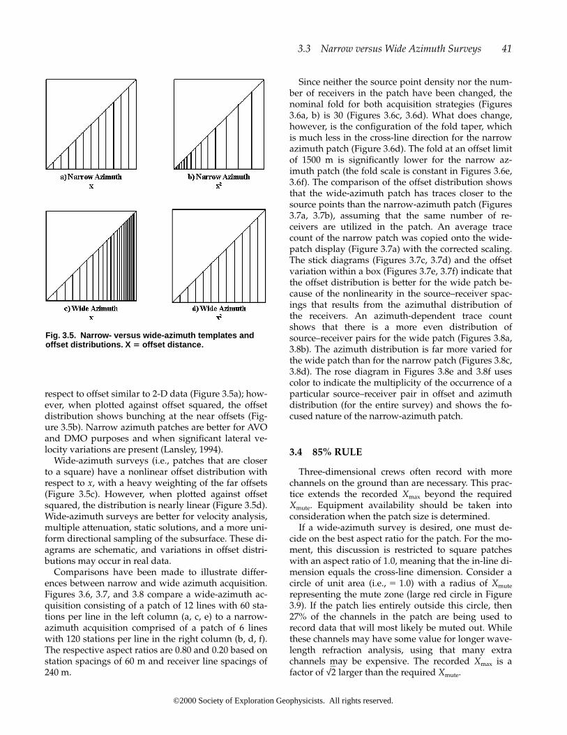
respect to offset similar to 2-D data (Figure 3.5a); how-ever, when plotted against offset squared, the offsetdistribution shows bunching at the near offsets (Fig-ure 3.5b). Narrow azimuth patches are better for AVOand DMO purposes and when significant lateral ve-locity variations are present (Lansley, 1994).
Wide-azimuth surveys (i.e., patches that are closerto a square) have a nonlinear offset distribution withrespect to x, with a heavy weighting of the far offsets(Figure 3.5c). However, when plotted against offsetsquared, the distribution is nearly linear (Figure 3.5d).Wide-azimuth surveys are better for velocity analysis,multiple attenuation, static solutions, and a more uni-form directional sampling of the subsurface. These di-agrams are schematic, and variations in offset distri-butions may occur in real data.
Comparisons have been made to illustrate differ-ences between narrow and wide azimuth acquisition.Figures 3.6, 3.7, and 3.8 compare a wide-azimuth ac-quisition consisting of a patch of 12 lines with 60 sta-tions per line in the left column (a, c, e) to a narrow-azimuth acquisition comprised of a patch of 6 lineswith 120 stations per line in the right column (b, d, f).The respective aspect ratios are 0.80 and 0.20 based onstation spacings of 60 m and receiver line spacings of240 m.
Since neither the source point density nor the num-ber of receivers in the patch have been changed, thenominal fold for both acquisition strategies (Figures3.6a, b) is 30 (Figures 3.6c, 3.6d). What does change,however, is the configuration of the fold taper, whichis much less in the cross-line direction for the narrowazimuth patch (Figure 3.6d). The fold at an offset limitof 1500 m is significantly lower for the narrow az-imuth patch (the fold scale is constant in Figures 3.6e,3.6f). The comparison of the offset distribution showsthat the wide-azimuth patch has traces closer to thesource points than the narrow-azimuth patch (Figures3.7a, 3.7b), assuming that the same number of re-ceivers are utilized in the patch. An average tracecount of the narrow patch was copied onto the wide-patch display (Figure 3.7a) with the corrected scaling.The stick diagrams (Figures 3.7c, 3.7d) and the offsetvariation within a box (Figures 3.7e, 3.7f) indicate thatthe offset distribution is better for the wide patch be-cause of the nonlinearity in the source–receiver spac-ings that results from the azimuthal distribution ofthe receivers. An azimuth-dependent trace countshows that there is a more even distribution ofsource–receiver pairs for the wide patch (Figures 3.8a,3.8b). The azimuth distribution is far more varied forthe wide patch than for the narrow patch (Figures 3.8c,3.8d). The rose diagram in Figures 3.8e and 3.8f usescolor to indicate the multiplicity of the occurrence of aparticular source–receiver pair in offset and azimuthdistribution (for the entire survey) and shows the fo-cused nature of the narrow-azimuth patch.
3.4 85% RULE
Three-dimensional crews often record with morechannels on the ground than are necessary. This prac-tice extends the recorded Xmax beyond the requiredXmute. Equipment availability should be taken intoconsideration when the patch size is determined.
If a wide-azimuth survey is desired, one must de-cide on the best aspect ratio for the patch. For the mo-ment, this discussion is restricted to square patcheswith an aspect ratio of 1.0, meaning that the in-line di-mension equals the cross-line dimension. Consider acircle of unit area (i.e., � 1.0) with a radius of Xmute
representing the mute zone (large red circle in Figure3.9). If the patch lies entirely outside this circle, then27% of the channels in the patch are being used torecord data that will most likely be muted out. Whilethese channels may have some value for longer wave-length refraction analysis, using that many extrachannels may be expensive. The recorded Xmax is afactor of larger than the required Xmute.√2
3.3 Narrow versus Wide Azimuth Surveys 41
Fig. 3.5. Narrow- versus wide-azimuth templates andoffset distributions. X � offset distance.
©2000 Society of Exploration Geophysicists. All rights reserved.

42 Patches and Edge Management
Fig. 3.6. Wide versus narrow patch—template and fold; a. wide-azimuth template, b. narrow-azimuth template, c. wide-azimuth fold distribution at full offsets, d. narrow-azimuth fold distribution at full offsets, e. wide-azimuth fold distribu-tion at 1500 m offsets, and f. narrow-azimuth fold distribution at 1500 m offsets.
©2000 Society of Exploration Geophysicists. All rights reserved.

3.3 Narrow versus Wide Azimuth Surveys 43
Fig. 3.7. Wide versus narrow patch—offset distribution; a. wide-azimuth offset distribution—trace count, b. narrow-azimuth offset distribution—trace count, c. wide-azimuth offset distribution—stick diagram, d. narrow-azimuth offsetdistribution—stick diagram, e. wide-azimuth offset distribution—offset variation within a box, and f. narrow-azimuthoffset distribution—offset variation within a box.
©2000 Society of Exploration Geophysicists. All rights reserved.

44 Patches and Edge Management
Fig. 3.8. Wide versus narrow patch—azimuth distribution; a. wide-azimuth azimuth distribution—trace count, b. nar-row-azimuth azimuth distribution—trace count, c. wide-azimuth azimuth distribution—spider diagram,d. narrow-az-imuth azimuth distribution—spider diagram, e. wide-azimuth azimuth distribution—rose diagram, and f. narrow-az-imuth azimuth distribution—rose diagram.
©2000 Society of Exploration Geophysicists. All rights reserved.

On the other hand, one can reduce the patch to lieentirely within the mute zone, as shown by the smallblue square. Xmax is now measured along the diagonalof the patch, but this patch covers only 64% of thearea of the design objective, i.e., the large red circle.This is the other extreme of inefficiency; there are onlya few traces that lie at offsets close to the ideal mutedistance. The recorded Xmax equals the required Xmute
in this case. Some companies select a patch size thatequals the large red square in order to record offsetsof Xmute in all directions. However, the large redsquare is twice the area of the small blue square, andthere is a significant difference in cost and effort be-tween the two patches.
The 85% Rule is a compromise and determines theaspect ratio of the patch relative to the desired Xmute.The 85% Rule is a simple way to optimize the area ofusable traces recorded and the number of channelsneeded. The rule works as follows (Figure 3.10):
1. Determine the desirable Xmute.2. Choose the in-line offset Xr to be 0.85 � Xmute.3. Choose the cross-line offset Xs to be 0.85 � Xr �
0.72 � Xmute.
For a real example with Xmute � 2000 m, (6600 ft)half in-line dimension
Xr � 85% � Xmute � 1700 m, (5610 ft)
half cross-line dimensionXs � 85% � Xr � 1445 m, (4730 ft)
aspect ratioXs � Xr � 85%.
The usable area of the patch relative to the circle ofXmute increases from 64% to 78%. Only a small part ofthe patch is outside the theoretical maximum offsetXmute (e.g., for a 6-line patch the traces at offsets greaterthan Xmute are less than 2.5%). Additional receiver linesfarther out than indicated by this patch are mostly out-side the usable offset Xmute. Therefore, the longer di-mension of the patch is preferred to be in the in-linedirection. The dimensions may need some slight ad-justment to be suitable for other considerations in thedesign of the 3-D. The recorded Xmax is 1.13 times therequired Xmute; most likely the mute affects only the farextremes of the two farthest receiver lines.
Referring back to Figure 3.9, the relationships be-tween the different areas are shown graphically inFigure 3.11. The red circle of radius Xmute has unit area(100% at 100% Xmute) and is shown as the solid line.The inner blue circle with a radius of 0.71 Xmute con-tains 50% of the area of the larger circle. If the patch isentirely within Xmute (inner blue square in Figure 3.9),then the curve describing its area deviates from the y � x2 form at 0.71 Xmute. The area of this smaller bluepatch is 64% of the unit area (red circle).
3.4 85% Rule 45
Fig. 3.9. Patc h dimension versus Xmute . Fig. 3.10. Ideal patch, using the 85% rule.
©2000 Society of Exploration Geophysicists. All rights reserved.

On the other hand, if the patch is entirely outsidethe red circle of Xmute (larger red square in Figure 3.9),then the curve describing its area deviates from the y � x2 trend at 100% Xmute. The area of this largerpatch is 127% of the unit area, which is twice the areaof the smaller patch, with its maximum offsets being141% of the mute offset. Therefore if one lays out re-ceivers in a square patch that has Xmax measured inthe in-line direction, then twice the number of re-ceivers are needed in comparison to a patch that hasXmax measured along the diagonal.
The patch using the 85% rule covers 78% of the unitarea described by the red circle of Xmute. The greenpatch covers an area that is 22% larger than thesmaller blue square (compare Figure 3.10). The patchusing the 85% rule is an excellent compromise for thepatch design with the recorded maximum offsets be-ing 113% of the required mute zone. The design pro-vides a sufficient number of large offsets, and only afew traces may have to be deleted in the stack.
3.5 FRESNEL ZONE
The Fresnel zone is that area of a reflector fromwhich reflected energy can reach a detector and notbe more than one-half wavelength out of phase withany other energy reflected from within that area(Sheriff, 1991). In Figure 3.12, energy traveling from asource at S to a subsurface point 0 arrives at the sur-face at time t0 � 2 � Z0 � Vave. Reflected energy frompoint A or A’ will reach the receiver at point 0 at timet1 � 2[(Z0 � Vave) � (� � 4Vave)]. All energy arrivingwithin the time interval (t1 – t0) interferes construc-tively.
The reflecting disk AA’ is called the first Fresnelzone (Sheriff, 1991). Two reflecting points that fallwithin this zone are generally considered indistin-guishable when observed at the earth’s surface. Theradius of the first Fresnel zone RF for vertical inci-dence can be approximated as
(3.1)
which can be further approximated by,
(3.2)
or
where fdom is the dominant frequency being consid-ered. At lower frequencies, the Fresnel zone becomeslarger, while for higher frequencies the Fresnel zone issmaller. This derivation follows the approach of Yil-maz (1987). For nonzero offset, structure and dip af-fect the shape of the Fresnel zone. Lindsey (1989)points out that the Fresnel zone becomes somewhatsmaller for positive structures such as reefs or anti-clines, and somewhat larger for negative structuressuch as synclines. Generally, this is a second-order ef-fect except when structures are of similar scale to thedepth.
The vertical thickness of the Fresnel zone ZF is
(3.4)ZF ��
4�
Vave
4 fdom
.
RF � 12Vave � t0
fdom�
1/2
,
RF � � Z0 � �
2 �1/2
� � t0 � Vave
2�
Vave
2 fdom�
1/2
RF � ��Z0 ��
4 �2
� Z02�
1/2
� � Z0 � �
2�
�2
16 �1/2
,
46 Patches and Edge Management
Fig. 3.11. Percentage of area covered for variouschoices of Xmute .
Fig. 3.12. Fresnel zone (after Yilmaz, 1987).
©2000 Society of Exploration Geophysicists. All rights reserved.
Expressing this in time, the two-way time thickness ofthe Fresnel zone TF becomes
(3.5)
where � is the wavelength of the dominant frequency.The diameter of the Fresnel zone determines the lat-
eral resolution before migration. In the context of dif-fractions, lateral resolution can be defined as the abil-ity to distinguish two adjacent diffractions. Becausemigration is a process that collapses diffractions, it isreasonable to think that migration increases spatialresolution. In effect, migration moves the plane of ob-servation downward to the reflection points. There-fore, the Fresnel zone becomes smaller (Yilmaz, 1987).Migration of 3-D data tends to collapse the Fresnelzone diameter to approximately one-half the domi-nant wavelength, while migration of 2-D data accom-plishes this only in the direction of the seismic line(Lindsey, 1989).
Migration introduces unwanted artifacts near theedges of the 3-D survey because part of the Fresnel zonelies outside the survey. These artifacts are of particularimportance when undershooting corners of lease blocks.
The above discussion considers only monochro-matic signals. Knapp (1991) proposed a generalizationof the Fresnel zone definition for broadband signalsthat guarantees the correct wavelet and amplitude ofthe reflected signal. Brühl et al. (1996) determined thatby comparing monochromatic, narrow band, andbroadband signals that the boundary of the (first)Fresnel zone corresponds to the position of maximumenergy build-up. Brühl et al. (1996) extended Knapp’sconcept to a “zone of influence,” because the size ofthe area that guarantees the correct wavelet dependson the length of the wavelet. By definition, the zone ofinfluence is the area on the reflector for which the dif-ference between the reflection traveltimes and the dif-fraction traveltimes is less than the length of thewavelet (rather than one half of the wavelength). Thisdefinition separates the reflected wavelet from the in-put wavelet. Any restriction of the reflector area to aradius smaller than that of the zone of influencewould result in a change of the reflected wavelet withrespect to the input wavelet.
3.6 DIFFRACTIONS
Diffractions occur where sharp reflector boundariesand discontinuities such as faults are present. Diffrac-tions extend far beyond and especially perpendicular
TF �
2 � �
4
Vave
��
2Vave
,
to faults. The migration apron needed to span thesediffractions adds to the surface coverage needed toimage the subsurface properly. Therefore, calculationsof migration apron need to be made prior to startingany 3-D design.
When source energy reaches a subsurface point dis-continuity (point diffractor), the reflected energy canbe ray traced upward to the surface at all angles.Wherever a receiver is positioned on the surface, itrecords a reflection corresponding to the time it takesfor the energy to travel from the source to the diffrac-tor plus the time it takes to travel upward. The collec-tion of all these various reflections along the receiverline creates a diffraction curve that has interestingproperties.
The area at the top of the diffraction curve that hasa thickness equal to one-quarter wavelength of thedominant frequency (or a two-way interval timeequal to one-half cycle of the dominant frequency) iscommonly called the first Fresnel zone. Other pointson the diffraction curve correspond to different raystraced from the diffractor to the surface at varying an-gles. Therefore, that part of the curve near its apexcorresponds to low scattering angles, and the parts ofthe curve at longer two-way times correspond togreater angles.
After migration, the diffraction curve (actually abell shape in 3-D) is collapsed, not quite to a spike asdescribed earlier, but to the highest frequency waveletin time and space permitted by the signal bandwidth.If only a portion of the diffraction curve can be used,the collapse will not be quite complete, and a mi-grated version of the event will contain only a fractionof the correct energy.
Using only the first Fresnel zone portion of a dif-fraction curve gives approximately 70% of the energyof the fully migrated result (the Fresnel zone corre-sponds approximately to a 15° scattering angle). Us-ing both sides of the diffraction out to a scattering an-gle of 30° gives approximately 95% of the fullymigrated result (Figure 3.13). The exact quantity (e.g.,95%, 96%, . . . ) depends on the velocities anddepths of the diffractors. The recording of a completediffraction curve is not necessary to get a useful mi-grated result.
3.7 MIGRATION APRON
Migration is necessary to place dipping horizonsand faults at their proper subsurface positions. Whendesigning the boundaries of a survey, the full-foldarea covered must be increased to allow for the mi-gration apron. The amount of increased area is not
3.7 Migration Apron 47
©2000 Society of Exploration Geophysicists. All rights reserved.

necessarily the same in the strike and the dip direc-tion. In a constant-velocity medium, dipping horizonsrequire a migration apron given by the following for-mula:
MA � Z tan �, (3.6)
where MA � migration apron, Z � depth, and � �
dip angle (true reflector dip).Assuming straight raypath geometry, if one wants
to record reflections from a horizon at a depth of 2000m (6500 ft) that dips 20°, then 728 m (2366 ft) need tobe added to the 3-D grid size as the migration apron.However, to capture the 30° ray off the outermostpoint of a diffraction, the migration apron must be atleast Z � tan 30° � 0.58 � Z as per Figure 3.13 (in theabove example, 0.58 � 2000 m � 1155 m or 0.58 �
6500 ft � 3753 ft). This condition defines the desiredmigration apron unless dips exceed 30°. Table 3.1 has constant migration apron values in the columnsfor 10°, 20°, and 30° because the diffraction criterion isthe constraining factor. In practice, cost considerationsoften force a compromise on this desired apron.Curved raypaths assumptions reduce the requiredmigration apron (Figure 3.14; Bee et al., 1994), espe-cially if large dips are present. The depth-varying ve-locity field should be taken into account when calcu-lating the size of the migration apron. Ray tracing
from an exploding reflector at depth can help deter-mine the required migration apron in a velocity lay-ered medium.
Rule of Thumb: Migration apron is normally chosen asthe larger of:
1) The lateral migration movement of each dip in the ex-pected geology, or
2) The distance required to capture diffraction energycoming upwards at a scattering angle of 30°, or
3) The radius of the first Fresnel zone.
Displays such as Figure 3.15 help determine verticalresolution (one-quarter wavelength of dominant fre-quency) and lateral resolution before migration (Fres-nel zone diameter versus bin size). Other displays al-low the selection of the bin size required to image adesired high frequency on certain dips in the model.The survey size should be calculated based on thearea to be imaged plus the migration apron.
3.8 EDGE MANAGEMENT
Edge management refers to the aspect of 3-D designthat specifies the width of the migration apron andthe fold taper. The fold taper is the area at the edge of
48 Patches and Edge Management
Fig. 3.13. Anatom y of a diffraction curve.Fig. 3.14. Width of migration apron for media having aconstant velocity field versus a linearly varying velocity(after Bee et al., 1994).
©2000 Society of Exploration Geophysicists. All rights reserved.

the survey where full-fold (or nearly full-fold) atdepth has not been reached before migration. Often asmall relaxation in the definition of sufficient foldnear the edges can significantly reduce the total sizeof the survey.
The fold taper can easily add 30% to the total 3-Darea, even on large surveys. On small surveys, thispercentage increases disproportionately and makessmall 3-D surveys, which might be intended to coveras little as 2.5 km2 (1 mi2), extremely expensive on acost-per-area basis. The design of the patch (and there-fore fold taper) is often different in the receiver line di-rection than in the source line direction because dipsmay change depending on the azimuth, and then the
3.8 Edge Management 49
migration apron changes with dip azimuth. Calcula-tions of the fold taper distances were introduced inChapter 2. Figure 3.16 shows the usable 3-D programsize (net of the fold taper) as a percentage of the totalprogram size for a target depth of 2000 m (6500 ft) andfold taper widths of 200 to 1600 m (660 to 5280 ft).
Generally, fold builds up faster in the cross-line di-rection than in the in-line direction. This is especiallytrue for narrow azimuth designs because the fold ta-per in the cross-line direction is directly proportionalto the cross-line fold. Careful distribution of receiverscan build up fold faster for certain geometries. Theorientation of the patch with respect to the surveyoutline can affect the cost of a survey significantly.
Diffractor Dip angle (degrees)
depth (ft) 10° 20° 30° 40° 50° 60° 70° 80° 90°
1000 577 577 577 839 1192 1732 2747 5671 ∞2000 1155 1155 1155 1678 2384 3464 5495 11343 ∞3000 1732 1732 1732 2517 3575 5196 8242 17014 ∞4000 2309 2309 2309 3356 4767 6928 10990 22685 ∞5000 2887 2887 2887 4195 5959 8660 13737 28356 ∞6000 3464 3464 3464 5035 7151 10392 16485 34028 ∞7000 4041 4041 4041 5874 8342 12124 19232 39699 ∞8000 4619 4619 4619 6713 9534 13856 21980 45370 ∞9000 5196 5196 5196 7552 10726 15588 24727 51042 ∞
10000 5774 5774 5774 8391 11918 17321 27475 56713 ∞11000 6351 6351 6351 9230 13109 19053 30222 62384 ∞12000 6928 6928 6928 10069 14301 20785 32970 68055 ∞13000 7506 7506 7506 10908 15493 22517 35717 73727 ∞14000 8083 8083 8083 11747 16685 24249 38465 79398 ∞15000 8660 8660 8660 12586 17876 25981 41212 85069 ∞
; Diffraction : ; Migration of dipping events :
Table 3.1. Migration apron calculations for a variety of target depths and structural dips.
a) Metric
Diffractor Dip angle (degrees)
depth (m) 10° 20° 30° 40° 50° 60° 70° 80° 90°
500 289 289 289 420 596 866 1374 2836 ∞1000 577 577 577 839 1192 1732 2747 5671 ∞1500 866 866 866 1259 1788 2598 4121 8507 ∞2000 1155 1155 1155 1678 2384 3464 5495 11343 ∞2500 1443 1443 1443 2098 2979 4330 6869 14178 ∞3000 1732 1732 1732 2517 3575 5196 8242 17014 ∞3500 2021 2021 2021 2937 4171 6062 9616 19849 ∞4000 2309 2309 2309 3356 4767 6928 10990 22685 ∞4500 2598 2598 2598 3776 5363 7794 12364 25521 ∞5000 2887 2887 2887 4195 5959 8660 13737 28356 ∞
; Diffraction : ; Migration of dipping events :
b) Imperial
©2000 Society of Exploration Geophysicists. All rights reserved.

Any 3-D survey should be considered as consistingof three zones (Figure 3.17). The first (innermost) zoneis the domain of the interpreter. All traces lying in thiszone should be considered full-fold and fully mi-grated. This is the image area the interpreter shouldlimit his examinations to and use as the basis for geo-logical interpretation. The second (middle) zone is acorridor around the innermost (image) zone. Theoreti-cally, the width of this corridor is equal to the migra-tion apron. In this corridor, the seismic processor as-
sembles full-fold stacked traces. Migration movesmost of the energy of these traces into the edge of theinnermost (image) zone. The third (outermost) zone isa corridor around the middle zone. The width of thiszone is the fold taper. In this corridor, the acquisition
50 Patches and Edge Management
Fig. 3.16. Usab le area of a 3-D survey versus totalrecorded area. Fig. 3.17. Three-zone acquisition model (theoretical).
Fig. 3-15. Modeling for Fresnel zone and migration apron.
©2000 Society of Exploration Geophysicists. All rights reserved.

planner places sources and receivers to ensure full-fold at the start of the middle (full-fold) zone. Theterm edge management implies the proper design ofthese three zones. Compromises can and almost al-ways will be made.
It is not necessary that traces in the middle zonehave near offsets. Farther traces contain deep data be-cause of NMO muting, but deep data migrate fartherlaterally. If the bins near the outside of the secondzone contain only far traces, and bins closest to the in-nermost zone contain more near traces (hence shallowdata), a good migrated result on the edge of the inner-most (image) zone should result at all depths.
It may also be possible to relax the 30° requirementfor very deep data. This concession reduces the size ofthe migration apron (Figure 3.18). Traces that are notquite full-fold may be acceptable for bins near the out-side edge of the middle zone. These traces correspondto the near 30° portion of the diffraction and do notcontribute much energy at the edge of the innermost(image) zone.
Rule of Thumb: In no case should the width of the totalmigration apron around the image area be less than theFresnel zone radius plus the full-fold taper size.
This design rule means there are full-fold tracesfrom the edge of the image area outward to one Fres-nel zone radius and lesser fold from there to the edgeof the survey. Most often, the migration apron and thefold taper blend together, and cost considerations in-fluence the final choices for a particular design. Ex-periments with models help identify these parametersin any specific project.
3.9 RAY-TRACE MODELING
So far, the term CMPs or common-midpoints hasbeen used. However, the energy returning from a reflec-tor does not necessarily originate from that point on thereflector that is halfway between source and receiver.Migration corrects traces from their CMP position to theCDP (common-depth-point) position. It is important toknow how well each piece of the target is illuminated,and not only what fold is achieved after migration. Thisimaging concept involves CDP fold. Three-dimensionalray tracing is essential for true CDP analysis.
Ray-trace modeling (Figure 3.19) is useful if the un-derlying geology is more complicated than the flat-layer model, and is often used for 3-D design. Examplesof situations where ray tracing should be done includesalt domes, faults, steeply dipping layers, and lateralvelocity discontinuities. Such modeling may lead thedesigner to a different strategy for the surface layoutthan do the flat-layer assumptions. Source and receiverspacing may be reduced or increased in certain areas ofthe seismic survey to assure coverage in structurallycomplex areas (Neff and Rigdon, 1994). Sophisticatedcomputer programs are available to evaluate illumina-tion fold distributions versus nominal fold in structured
3.9 Ray-Trace Modeling 51
Fig. 3.18. Practical edge management.
Fig. 3.19. Rays belonging to one source point after 3-Dray tracing of a salt layer (Cain et al., 1998).
©2000 Society of Exploration Geophysicists. All rights reserved.

environments (Cain et al., 1998). The fold can be drapedover the structural elements of Figure 3.19 and the illu-mination is evaluated for the target horizons (Figure3.20). Some salt flanks have not been illuminated at all,which hinders the interpretation severely. The impact ofvarying fold and offset and azimuth distributions canbe rigorously evaluated with these programs.
3.10 RECORD LENGTH
The total record length needs to include several ar-rival times. First, the vertical two-way time to themain target can easily be obtained from existing 2-D
data. Second, the record length should be chosen sothat any diffraction patterns from the deepest event ofinterest (which may include basement) are properlyrecorded suitable for migration.
Margrave (1997) summarized these ideas for con-stant-velocity situations (Figure 3.21) and showed thatthe record length has to be at least:
(3.7)
where � is the scattering angle between the verticalaxis and the farthest receiver to be recorded.
Third, the moveout times for reflectors and multi-ples have to be taken into account at the far offsets. Fi-nally, static shifts may require up to 100 ms more andinstrumentation requirements add an additional100–200 ms. Therefore the total required recordlength is significantly more than simply the two-waytime to the main target.
For example, assume that existing 2-D data showthat the target horizon is at 1.5 s. Furthermore, as-sume that it is desirable to image basement, which isat 2.5 s. Diffraction tails are on the order of 500 ms,moveout is assumed to add 300 ms, dip requirementsmay add 400 ms, static shifts may require up to 100ms, and instrumentation requirements are 100 to 200ms. Although there is some overlap among these re-quirements, one would probably choose a recordingtime of 3.5 to 4.0 s.
It is always easy to record longer trace data becausetape is usually cheap in comparison to other recordingcosts. The only concern might be with telemetry sys-tems, where a longer record length may slow downthe overall acquisition effort because of the necessity
t �2Z
V cos �,
52 Patches and Edge Management
Fig. 3.21. Recor d length t as a function of scattering an-gle � (after Margrave, 1997).
Fig. 3.22a. Constant velocity scattering angle chartshowing: aperture limit, record length limit, and spatialaliasing limit for a case when Xmax � 2500 m, t � 3.0 s,V � 3500 m/s, B � 20 m, and f � 60 Hz (after Margrave,1997).
Fig. 3.20. 3-D illumination fold map for salt layer (Cainet al., 1998).
©2000 Society of Exploration Geophysicists. All rights reserved.

to transmit the information from each station sequen-tially after the shot has been taken. This limitation hasbeen reduced with recent product enhancements.
Margrave (1997) has described how the recordlength, the far-offset limit (as defined by Xmax), andspatial aliasing limit the maximum scattering anglethat can be recorded for the constant velocity case andstraight raypaths (Figure 3.22a), as well as the depthvarying velocity case Vz and curved raypaths (Figure3.22b). Such displays can be created for other velocityfields, recording times, maximum offsets, bin sizes,and maximum frequencies.
Let’s Design a 3-D – Part 3 (metric)
In this example, these are the following known para-meters:
existing 2-D data of goodquality have 30 fold
steepest dips 20°shallow markers needed for
isochroning have 500 m offsetstarget depth 2000 mtarget two-way time 1.5 sbasement depth 3000 mVint immediately above the
target horizon 4200 m/sfdom at the target horizon 50 Hzfmax at the target horizon 70 Hzlateral target size 300 m
Orthogonal method is to be used.
Desired Fold:
up to full 2-D fold � 15–3012
Bin size:
a) for target size: B � 300 m � 3 � 100 mb) for alias frequency: B � Vint � (4 � fmax � sin �)
� 4200 m/s � (4 � 70 Hz � sin 20°)� 44 m
c) For lateral resolution: B � Vint � (N � fdom) �
4200 m/s � (N � 50 Hz) � 21 to 42 mbin size � 30 m � 30 mRI � 60 mSI � 60 m
Desired Xmin: 500 m
RLI � 360 mSLI � 360 mXmin � (3602
� 3602)1/2 m � 509 m(467 m with one bin offset at line intersections)
Desired Xmute: 2000 m
patch 8 � 60 or 2880 m � 3600 mnumber of channels � 480aspect ratio � 2880 � 3600 � 0.80Xmax � � (28802 + 36002)1/2 m � 2305 m
Fold:
in-line fold � 60 m � 60 m � (2 � 360 m) � 5cross-line fold � 8 � 2 � 4total fold � 20
Migration Apron:
radius of Fresnel Zone �
� Vave � (target two-way time � fdom)1/2 �
diffraction energy � 0.58 � target depth �
migration apron � target depth � tan (dip) �
in-line fold taper �
[(in-line fold � 2) � 0.5] � SLI �
cross-line fold taper �
[(cross-line fold � 2) � 0.5] � RLI �(FT � FZ) total migration apron (FT � MA)TMA range �
Let’s Design a 3-D—Part 3 (imperial)
In this example, these are the following known parameters:
existing 2-D data of good quality have 30 fold
steepest dips 20°shallow markers needed for
isochroning have 1500 ft offsetstarget depth 6000 fttarget two-way time 1.5 s
12
12
3.10 Record Length 53
Fig. 3.22b. Constant gradient scattering angle chartshowing: aperture limit, record length limit, and spatialaliasing limit for a case when Xmax � 2500 m, t � 3.0 s,V � 1500 m/s � 0.6 � Z m/s, B � 20 m, and f � 60 Hz(after Margrave, 1997).
©2000 Society of Exploration Geophysicists. All rights reserved.

basement depth 10 000 ftVint immediately above the target
horizon 14 000 ft/sfdom at the target horizon 50 Hzfmax at the target horizon 70 Hzlateral target size 1000 ft
Orthogonal method is to be used.
Desired Fold:
up to full 2-D fold � 15–30
Bin size:
a) for target size: B � 1000 ft � 3 � 333 ftb) for alias frequency: B � Vint � (4 � fmax � sin �)
� 14 000 ft/s � (4 � 70 Hz � sin 20°) � 146 ftc) for lateral resolution: B � Vint � (N � fdom) �
14 000 ft/s � (N � 50 Hz)� 70 to 140 ft
bin size � 110 ft � 110 ftRI � 220 ftSI � 220 ft
Desired Xmin: ~1500 ft
RLI � 880 ftSLI � 1320 ftXmin � (8802
� 13202)1/2 ft � 1586 ft (1434 with one bin offset at line intersections)
Desired Xmute: ~6000 ft
patch 10 � 48 or 8800 ft � 10 560 ftnumber of channels � 480aspect ratio � 8800 � 10 560 � 0.83Xmax � � (88002
� 10 5602)1/2 ft � 6873 ft
Fold:
in-line fold � 48 � 220 ft � (2 � 1320 ft ) � 4cross-line fold � 10 � 2 � 5total fold � 20
Migration Apron:
radius of Fresnel Zone �
� Vave � (target two-waytime � fdom)1/2 �
diffraction energy � 0.58 � target depth �migration apron � target depth � tan (dip) �in-line fold taper � [(in-line fold � 2) – 0.5] � SLI �
cross-line fold taper � [(cross-line fold � 2) – 0.5]
12
12
12
� RLI � (FT � FZ) total migration apron (FT � MA) TMA range �
Let’s Design a 3-D—Summary (metric)
In this example, these are the following known pa-rameters:
existing 2-D data of good quality have 30 fold
steepest dips 20°shallow markers needed for
isochroning have 500 m offsetstarget depth 2000 mtarget two-way time 1.5 sbasement depth 3000 mVint immediately above the
target horizon 4200 m/sfdom at the target horizon 50 Hzfmax at the target horizon 70 Hzlateral target size 300 m
Orthogonal method is to be used.
Desired Fold:
up to full 2-D fold � 15 � 30
Bin size:
a) for target size: B � 300 m � 3 � 100 mc) for alias frequency:
B � Vint � (4 � fmax � sin �)� 4200 m/s � (4 � 70 Hz � sin 20°) � 44 m
c) for lateral resolution: B � 4200 m/s � (N � 50 Hz)
� 21 to 42 mbin size � 30 m � 30 mRI � 60 mSI � 60 m
Desired Xmin: 500 m
RLI � 360 mSLI � 360 mXmin � (3602
� 3602)1/2 m � 509 m(467 m with one bin offset at line intersections)
Desired Xmute: 2000 m
patch 8 � 60 or 2880 m � 3600 mnumber of channels � 480aspect ratio � 2880 � 3600 � 0.80Xmax � � (28802
� 36002)1/2 m � 2305 m12
12
54 Patches and Edge Management
©2000 Society of Exploration Geophysicists. All rights reserved.

Fold:
in-line fold � 60 � 60 m � (2 � 360 m) � 5cross-line fold � 8 � 2 � 4total fold � 20
Migration Apron:
radius of Fresnel Zone � � 2666 m/s � (1.5 s ÷50 Hz)1/2 � 231 m
diffraction energy � 0.58 � 2000 m � 1155 mmigration apron � 2000 � tan 20° � 728 min-line fold taper � [(in-line fold � 2) � 0.5] � SLI� 2.0 � 360m � 720 mcross-line fold taper � [(cross-line fold � 2) � 0.5]� RLI � 1.5 � 360 � 540 mTMA range � 771 m to 1875 m
Let’s Design a 3-D – Summary (imperial)
In this example, these are the following known parameters:
existing 2-D data of good quality have 30 foldsteepest dips 20°shallow markers needed for
isochroning have 1500 ft offsetstarget depth 6000 fttarget two-way time 1.5 sbasement depth 10 000 ftVint immediately above the target
horizon 14 000 ft/sfdom at the target horizon 50 Hzfmax at the target horizon 70 Hzlateral target size 1000 ft
Orthogonal method is to be used.
Desired Fold:
up to full 2-D fold � 15–30
Bin size:
c) for target size: B � 1000 ft � 3 � 333 ftd) for alias frequency:
B � Vint � (4 � fmax � sin (dip)) � 14 000 ft/s � (4 � 70 Hz � sin 20°) � 146 ft
c) for lateral resolution: B � Vint � (N � fdom ) �
14 000 ft/s � (N � 50 Hz)� 70 to 140 ft
12
12
Bin size � 110 ft � 110 ftRI � 220 ftSI � 220 ft
Desired Xmin: ~1500 ft
RLI � 880 ftSLI � 1320 ftXmin � (8802 + 13202)1/2 ft � 1586 ft (1434 ft with onebin offset at line intersections)
Desired Xmute : ~6000 ft
patch 10 � 48 or 8800 ft � 10 560 ftnumber of channels � 480aspect ratio � 8800 � 10 560 � 0.83Xmax � � (88002
� 10 5602)1/2 ft � 6873 ft
Fold:
in-line fold � 48 � 220 ft � (2 � 1320 ft ) � 4cross-line fold � 10 � 2 � 5total fold � 20
Migration Apron:
radius of Fresnel Zone �
� 8000 ft/s � (1.5 s ÷ 50 Hz)1/2 � 693 ftdiffraction energy � 0.58 � 6000 ft � 3464 ftmigration apron � 6000 ft � tan 20° � 2184 ftin-line fold taper � [(in-line fold � 2) � 0.5] � SLI �
1.5 � 1320 ft � 1980 ftcross-line fold taper � [(cross-line fold � 2) � 0.5] �
RLI � 2 � 880 ft � 1760 ftTMA range � 2453 ft � 5444 ft
Chapter 3 Quiz
1. Is a wide azimuth survey or a narrow azimuth 3-D survey preferred for AVO work?
2. Based on diffraction energy, how large shouldthe migration apron be?
3. Should the migration apron have the same di-mension on all sides of the survey?
4. What are the three zones of the acquisitionmodel, and what type of data is contained ineach?
12
12
3.10 Record Length 55
©2000 Society of Exploration Geophysicists. All rights reserved.

©2000 Society of Exploration Geophysicists. All rights reserved.
4.1 3-D DESIGN FLOWCHART
Chapters 2 and 3 developed a fairly standard 3-Ddesign example. The decision-making order used inthat example works well for most 3-D design prob-lems. Survey design Table 2.1 should be reviewed asthe material in this chapter is considered, because thattable summarizes the criteria that can be used to de-termine the seven key parameters of 3-D design: fold,bin size, Xmin , Xmax , migration apron, fold taper, andrecording time. The required input parameters for a 3-D survey are summarized in Table 4.1. If one cannotdetermine all the starting parameters from explo-ration objectives and previous 2-D seismic data in thearea, then some reasonable estimates may suffice.
The flowchart in Table 4.1 should give a reason-able starting design in most cases. Once a startingdesign has been established, the source type should
be selected, and constraints such as surface condi-tions, costs, and operational considerations shouldbe addressed. For a large survey, operational andcost considerations may determine the final choice ofdesign. There are many layout strategies (Chapter 5)that can be used to good advantage in certain situa-tions. This flowchart is written for orthogonal de-signs, but it can be adapted in most cases to otherdesign strategies.
4.2 BASIC 3-D EQUATIONS—SQUAREBINS
The basic 3-D equations can be expressed in termsof the following parameters:
SD � source densityNC � number of recording channels in a patchB � bin sizeXr � in-line dimension of the patchXs � cross-line dimension of the patchRLI � receiver line intervalSLI � source line interval
U � units factor (10�6 for m/km2; 0.03587 � 10�6
for ft/mi2)
Chapters 2 and 3 derived the basic fold equation for3-D surveys. If the bin area � B2, then Fold � SD �
NC � B2� U (midpoints per bin) and
(4.1)SD �Fold
NC � B2� U
.
A � aspect ratio �Xs
Xr
57
4Flowcharts, Equations, and Spreadsheets
Table 4.1. 3-D design input parameters.
Determine the following parameters from exploration ob-jectives and from existing 2-D seismic data:
fold of good 2-D datasteepest dipmute for shallow markers needed for isochroningtarget depth and mute distancetarget two-way timemute for basement depth and mute distanceVint immediately above the target horizonfdom at the target horizonfmax at the target horizonlateral target size area to be fully imagedlayout method.
©2000 Society of Exploration Geophysicists. All rights reserved.

Example: Fold � 24, NC � 480,bin size B � 25 m (82.5 ft)
or
Equation (4.1) is the fundamental relationship gov-erning all 3-D surveys, regardless of the design strategy.There is an assumption in this derivation that recordingSD sources per unit area into NC channels gives rise toSD � NC midpoints inside the unit area. This assump-tion will be realized in practice only if some of the mid-points arise from sources outside the unit area and re-
� 205 sources/mi2
SD �24
480 � 82.52� 0.03587 � 10�6
SD �24
480 � 252� 10�6
� 80 sources/km2
ceivers inside the unit area under consideration andvice versa. This requirement implies that the receiverpatches and the sources fired into each patch must cre-ate overlapping areas of midpoints arranged in a regu-lar pattern. Such overlap ensures that there are SD �
NC midpoints in each unit area of the survey. Figure 4.1shows several overlapping midpoint areas that con-tribute to the fold in the central area.
If the receiver patches move (roll-along) in such away that there is insufficient overlap, one observesstripes of lower fold at regular intervals in the survey(see Chapter 9). This striping also occurs if some ofthe receivers are at offsets � Xmute and are not used inprocessing, e.g., for shallower horizons and smallermute distances.
The receiver line interval can be calculated as
(4.2)RLI �Xr � Xs
NC � 2B.
58 Flowcharts, Equations, and Spreadsheets
Table 4.2. 3-D design flowchart.
Desired Fold ( to 1) X full 2-D fold � _________
Bin size a) for target size: B � _________b) for alias frequency: B � Vint � (4 � fmax � sin �) � _________c) for lateral resolution: B � Vint � (N � fdom),
(N � 2 to 4) � _____ to _____bin size � _________RI � _________SI � _________
Desired Xmin : _________ RLI � _________SLI � _________Xmin � (RLI2
� SLI 2)1/2� _________
Desired Xmax: _________ number of channels in patch � _________number of receiver lines � _________channels per line � _________cross-line dimension � _________in-line dimension � _________aspect ratio � cross-line dimension of the patch/
in-line dimension of the patch � _________Xmax � � (in-line dimension of the patch)2
�
(cross-line dimension of the patch)2� _________
Fold: in-line fold � RLL � (2 � SLI ) � _________cross-line fold � NRL � _________total fold � _________
Migration Apron: radius of Fresnel Zone � � Vave � (target two-way time � fdom)1/2
� diffraction energy � 0.58 � target depth �
Migration apron � target depth � tan (dip) �
in-line fold taper � [(in-line fold � 2) � 0.5] � SLI �
cross-line fold taper � [(cross-line fold � 2) � 0.5] � RLI �
(FT � FZ) total migration apron (FT � MA)TMA �
12
12
12
12
12
©2000 Society of Exploration Geophysicists. All rights reserved.

Example: Xmax � 2300 m (7500 ft), so Xr � Xs � 3200m (10 600 ft) and assuming NC � 480, B � 25 m(82.5 ft), A � 1
or
This expression links RLI and NC. The assump-tions are: a rectangular receiver patch with receiversspaced 2B apart and NC receivers in an area with dimensions Xr � Xs ; receivers are laid out as paral-lel lines that are RLI apart; and all NC channels liewithin a useful offset range. These assumptions arenot overly rigid. ARCO button patch designs fall into this scheme if one assumes that half the patch isempty. In other words, the button patch designshould be calculated using 2 � NC channels insteadof NC.
The number of receiver lines follows from the cross-line dimension of the patch and the receiver line inter-val; i.e.,
(4.3)NRL �Xs
RLI.
RLI �Xr � Xs
NC � 2B�
10 6002
480 � 2 � 82.5� 1419 ft.
RLI �Xr � Xs
NC � 2B�
32002
480 � 2 � 25� 427 m
From equations (4.2) and (4.3),
(4.4)
and combining equations (4.1) and (4.2) results in
(4.5)
The source line interval can be calculated from:
(4.6)
Important geometrical considerations are to deter-mine how NS sources per square kilometer (mile) canbe laid out because there must be 1000 � 2B sourcesper line km (5280 � 2B sources per line mile). The SLIvalue can be thought of as sources per km2 (mi2) di-vided by sources per line km (mi).
4.3 BASIC 3-D EQUATIONS—RECTANGULAR BINS
If the CMP bins are rectangular, the preceding binsize B needs to be replaced with:
Bs � bin size in direction of source linesBr � bin size in direction of receiver lines
The fundamental design equations are then as fol-lows. First,
(4.7)
This equation assumes 100% overlapping patternsin each area of the survey, or a regular midpoint den-sity. Second,
(4.8)
This equation assumes a rectangular receiver patchwith receiver stations spaced 2Br apart and NC re-ceivers in area Xr � Xs . Other key equations are
(4.9)
(4.10)RLI �SD � Xr � Xs � Br � U
Fold,
NRL �NC � 2Br
Xr
,
RLI �Xr � Xs
NC � 2Br
.
SD �Fold
NC � Bs � Br � U.
SLI �1
2B � SD � U.
RLI �SD � Xr � Xs � B � U
2 � Fold.
NRL �NC � 2B
Xr
,
4.4 Basic Steps in 3-D Layout—Five-Step Method 59
Fig. 4.1. Overlapping midpoint areas.
©2000 Society of Exploration Geophysicists. All rights reserved.
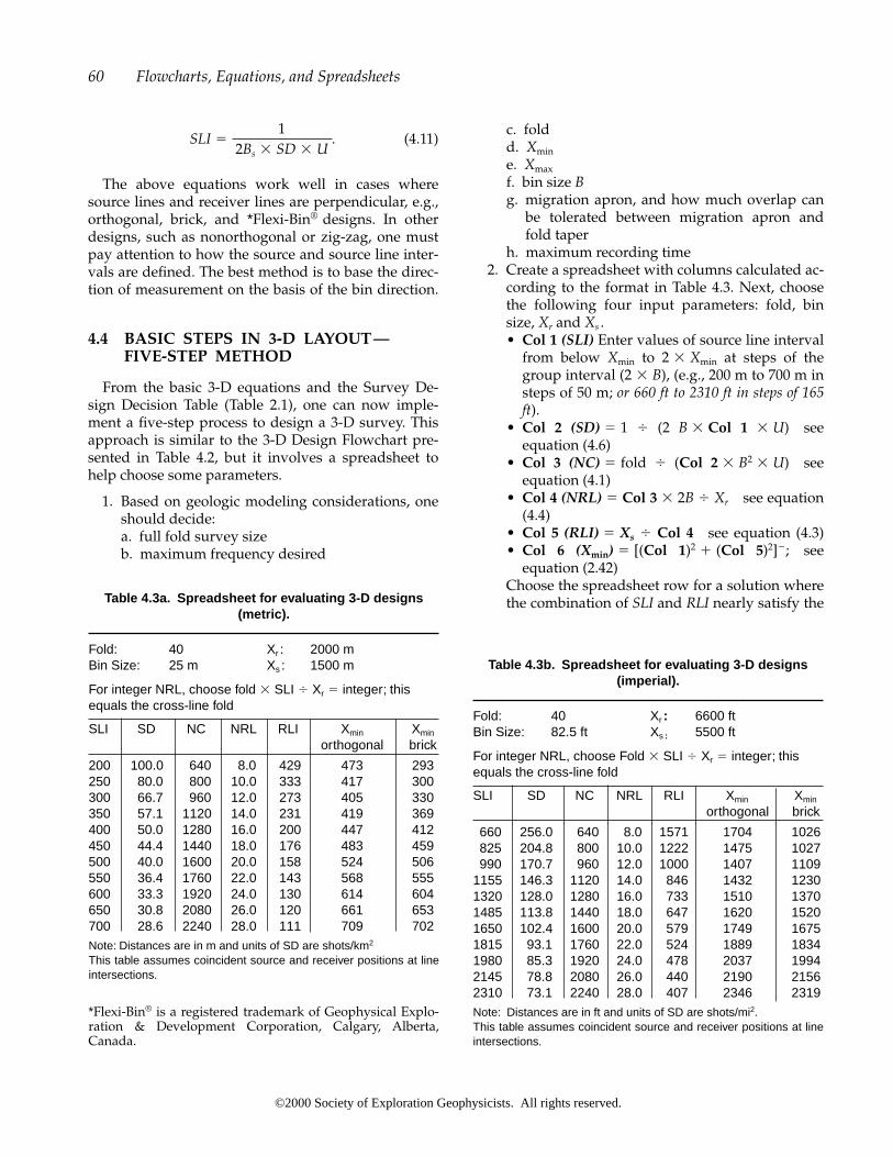
(4.11)
The above equations work well in cases wheresource lines and receiver lines are perpendicular, e.g.,orthogonal, brick, and *Flexi-Bin® designs. In otherdesigns, such as nonorthogonal or zig-zag, one mustpay attention to how the source and source line inter-vals are defined. The best method is to base the direc-tion of measurement on the basis of the bin direction.
4.4 BASIC STEPS IN 3-D LAYOUT—FIVE-STEP METHOD
From the basic 3-D equations and the Survey De-sign Decision Table (Table 2.1), one can now imple-ment a five-step process to design a 3-D survey. Thisapproach is similar to the 3-D Design Flowchart pre-sented in Table 4.2, but it involves a spreadsheet tohelp choose some parameters.
1. Based on geologic modeling considerations, oneshould decide:a. full fold survey sizeb. maximum frequency desired
SLI �1
2Bs � SD � U.
c. foldd. Xmin
e. Xmax
f. bin size Bg. migration apron, and how much overlap can
be tolerated between migration apron andfold taper
h. maximum recording time2. Create a spreadsheet with columns calculated ac-
cording to the format in Table 4.3. Next, choosethe following four input parameters: fold, binsize, Xr and Xs .• Col 1 (SLI) Enter values of source line interval
from below Xmin to 2 � Xmin at steps of thegroup interval (2 � B), (e.g., 200 m to 700 m insteps of 50 m; or 660 ft to 2310 ft in steps of 165ft).
• Col 2 (SD) � 1 � (2 B � Col 1 � U) seeequation (4.6)
• Col 3 (NC) � fold � (Col 2 � B2� U) see
equation (4.1)• Col 4 (NRL) � Col 3 � 2B � Xr see equation
(4.4)• Col 5 (RLI) � Xs � Col 4 see equation (4.3)• Col 6 (Xmin) � [(Col 1)2
� (Col 5)2]�; seeequation (2.42)
Choose the spreadsheet row for a solution wherethe combination of SLI and RLI nearly satisfy the
60 Flowcharts, Equations, and Spreadsheets
Table 4.3a. Spreadsheet for evaluating 3-D designs(metric).
Fold: 40 Xr : 2000 mBin Size: 25 m Xs : 1500 m
For integer NRL, choose fold � SLI � Xr � integer; thisequals the cross-line fold
SLI SD NC NRL RLI Xmin Xmin
orthogonal brick
200 100.0 640 8.0 429 473 293250 80.0 800 10.0 333 417 300300 66.7 960 12.0 273 405 330350 57.1 1120 14.0 231 419 369400 50.0 1280 16.0 200 447 412450 44.4 1440 18.0 176 483 459500 40.0 1600 20.0 158 524 506550 36.4 1760 22.0 143 568 555600 33.3 1920 24.0 130 614 604650 30.8 2080 26.0 120 661 653700 28.6 2240 28.0 111 709 702Note: Distances are in m and units of SD are shots/km2
This table assumes coincident source and receiver positions at lineintersections.
Table 4.3b. Spreadsheet for evaluating 3-D designs (imperial).
Fold: 40 Xr : 6600 ftBin Size: 82.5 ft Xs : 5500 ft
For integer NRL, choose Fold � SLI � Xr � integer; thisequals the cross-line fold
SLI SD NC NRL RLI Xmin Xmin
orthogonal brick
660 256.0 640 8.0 1571 1704 1026825 204.8 800 10.0 1222 1475 1027990 170.7 960 12.0 1000 1407 1109
1155 146.3 1120 14.0 846 1432 12301320 128.0 1280 16.0 733 1510 13701485 113.8 1440 18.0 647 1620 15201650 102.4 1600 20.0 579 1749 16751815 93.1 1760 22.0 524 1889 18341980 85.3 1920 24.0 478 2037 19942145 78.8 2080 26.0 440 2190 21562310 73.1 2240 28.0 407 2346 2319Note: Distances are in ft and units of SD are shots/mi2.This table assumes coincident source and receiver positions at lineintersections.
*Flexi-Bin® is a registered trademark of Geophysical Explo-ration & Development Corporation, Calgary, Alberta,Canada.
©2000 Society of Exploration Geophysicists. All rights reserved.

near-offset (Xmin) constraint. Select a receiver lineinterval that is smaller than necessary for the re-quired Xmin and that is a multiple of the stationinterval. Adjust Xr and Xs within reasonablebounds for the desired stacking offset to create apatch with an even number of receiver lines. Toachieve an even number of receiver lines, the ex-pression, fold � SLI � Xr must be an integer(this quantity is the cross-line fold).
3. Choose a layout strategy such as orthogonal line,depending on practical considerations such asaccess and available equipment. Add exclusionzones and move source and receiver lines to ac-commodate real-life features. Move and addsources where necessary to preserve fold, offset,and azimuth mix. Determine migration and foldtaper needs.
4. Model the 3-D survey for fold, offset and az-imuth variations, as well as edge management.Numerous quality control displays should bemade to assure a high-quality acquisition.
5. Prepare preplots and script files for the field op-erations.
Other methods are possible, but equation (4.1) [NS �
Fold � (NC � B2� U)] is fundamental to any 3-D
layout strategy.
4.5 GRAPHICAL APPROACH
The requirements for a graphical approach to 3-Ddesign are as follows:
Fold � 25, B � 25 m,Xr � Xs � 5000 m with Xmax � 3500 m, A � 1
or
Fold � 25, B � 82.5 ft,Xr � Xs � 16 500 ft with Xmax � 11 550 ft, A � 1
Two equations limit the source density SD. The firstequation relates SD to RLI:
SD �2 � Fold � RLI
Xs � Xr � B � U� 0.08 � RLI
4.5 Graphical Approach 61
[See equation (4.9) and graph U of Figure 4.2a]
or � 0.0621 � RLI.
The second equation relates SD to NC:
[See equation (4.1) and graph of Figure 4.2b]
or
Assume that 700 m (2310 ft) is the largest minimumacceptable offset Xmin in any bin. This requirement canbe achieved with RLI in the range of 250 to 600 m (825to 1980 ft).
To achieve these parameters (Fold � 25, B � 25 m,Xr � Xs � 5000 m, RLI � 250-650 m or Fold � 25, B �
82.5 ft, Xr � Xs � 16 500 ft, RLI � 825 to 1980 ft), NShas to be in the range of 20 to 52 sources/km2 (51 to123 sources/mi2), and NC has to be in the range of 770to 2000 (833 to 2008) channels.
In this case SLI � 400 to 1000 m (1320 to 3300 ft)[from equation (4.11)]. To optimize Xmin , SLI shouldbe as close to the receiver line interval as possible. IfRLI � SLI � 500 m, then Xmin is 700 m/(1760 ft, thenXmin is 2489 ft), SD � 40 sources/km2 (96 sources/mi2),and NC � 1000 (1066) channels.
NS �102 400
NC.
SD �Fold
NC � B2� U
�40 000
NC
Fig. 4.2. Graphical determination of acquisistion para-meters.
©2000 Society of Exploration Geophysicists. All rights reserved.

The solutions that are presented are limited to typi-cal designs used for land 3-D surveys with an aspectratio 1.0. In a spreadsheet form, one can makechanges to suit each prospect environment. Suchspreadsheets allow a quick review of several solutionswith the associated minimum and maximum offsetsas well as the aspect ratios. The tables in Section 4.6
62 Flowcharts, Equations, and Spreadsheets
4.6 STANDARDIZED SPREADSHEETS
A simple way to review numerous design choices isto create standardized spreadsheets that are based onfold and bin size as follows:
assume that the lines were shifted by one bin sizefrom their coincident positions at the line intersec-tions. Note that the receiver line interval can bechanged without affecting the fold; however, the min-imum and maximum offsets, as well as the aspect ra-tios, would be changed. Design 13 is one of the possi-ble solutions for the “Let’s Design a 3-D” exercises.
Bin Size 30 m 20 fold
Design RI SI RLI SLI Channels Lines Fold Xmin Xmax Aspect(m) (m) m) (m) (m) (m) ratio
1 60 60 120 120 160 8 20 127 768 0.802 60 60 120 180 240 10 20 175 937 0.833 60 60 120 240 320 10 20 228 1132 0.634 60 60 180 180 240 8 20 212 1152 0.805 60 60 180 240 320 10 20 258 1316 0.946 60 60 180 300 400 10 20 309 1500 0.757 60 60 240 240 320 8 20 297 1537 0.808 60 60 240 300 400 10 20 342 1697 1.009 60 60 240 360 480 10 20 391 1874 0.83
10 60 60 300 300 400 8 20 382 1921 0.8011 60 60 300 360 480 8 20 426 2163 0.6712 60 60 300 420 560 8 20 474 2252 0.8913 60 60 360 360 480 8 20 467 2305 0.8014 60 60 360 480 640 10 20 558 2632 0.9415 60 60 480 480 640 8 20 636 3073 0.8016 60 60 480 600 800 10 20 726 3394 1.0017 60 60 480 720 960 10 20 824 3749 0.8318 60 60 600 600 800 8 20 806 3842 0.8019 60 60 720 720 960 8 20 976 4610 0.8020 60 60 960 960 1280 8 20 1315 6147 0.80
©2000 Society of Exploration Geophysicists. All rights reserved.

The same table can be converted to imperial units:
The following pages summarize numerous solu-tions for orthogonal 3-D surveys. These solutions al-
4.6 Standardized Spreadsheets 63
Bin Size 110 ft 20 fold
Design RI SI RLI SLI Channel Lines Fold Xmin Xmax Aspect(ft) (ft) (ft) (ft) (ft) (ft) ratio
1 220 220 440 440 160 8 20 467 2817 0.802 220 220 440 660 240 10 20 641 3437 0.833 220 220 440 880 320 10 20 838 4151 0.634 220 220 660 660 240 8 20 778 4226 0.805 220 220 660 880 320 10 20 946 4825 0.946 220 220 660 1100 400 10 20 1133 5500 0.757 220 220 880 880 320 8 20 1089 5635 0.808 220 220 880 1100 400 10 20 1254 6223 1.009 220 220 880 1320 480 10 20 1434 6873 0.83
10 220 220 1100 1100 400 8 20 1400 7043 0.8011 220 220 1100 1320 480 8 20 1563 7932 0.6712 220 220 1100 1540 560 10 20 1739 8258 0.8913 220 220 1320 1320 480 8 20 1711 8452 0.8014 220 220 1320 1760 640 10 20 2046 9650 0.9415 220 220 1760 1760 640 8 20 2333 11269 0.8016 220 220 1760 2200 800 10 20 2663 12445 1.0017 220 220 1760 2640 960 10 20 3020 13746 0.8318 220 220 2200 2200 800 8 20 2956 14087 0.8019 220 220 2640 2640 960 8 20 3578 16904 0.8020 220 220 3520 3520 1280 8 20 4822 22539 0.80
Design 9 is one of the possible answers for the “Let’s Design a 3-D” exercises.
Bin Size 25 m 12 fold
Design RI SI RLI SLI Channels Lines Fold Xmin Xmax Aspect(m) (m) (m) (m) (m) (m) ratio
1 50 50 100 100 96 6 12 106 500 0.752 50 50 100 150 144 8 12 146 602 0.893 50 50 100 200 192 8 12 190 721 0.674 50 50 150 150 144 6 12 177 750 0.755 50 50 150 200 192 8 12 215 849 1.006 50 50 150 250 240 8 12 257 960 0.807 50 50 200 200 192 6 12 247 1000 0.758 50 50 200 250 240 6 12 285 1166 0.609 50 50 200 300 288 8 12 326 1204 0.89
10 50 50 250 250 240 6 12 318 1250 0.7511 50 50 250 300 288 6 12 355 1415 0.6312 50 50 250 350 336 8 12 395 1450 0.9513 50 50 300 300 288 6 12 389 1500 0.7514 50 50 300 400 384 8 12 465 1697 1.0015 50 50 400 400 384 6 12 530 2000 0.7516 50 50 400 500 480 6 12 605 2332 0.6017 50 50 400 600 576 8 12 686 2408 0.8918 50 50 500 500 480 6 12 672 2500 0.7519 50 50 600 600 576 6 12 813 3000 0.7520 50 50 800 800 768 6 12 1096 4000 0.75
low the selection of suitable 3-D designs for a varietyof different situations.
©2000 Society of Exploration Geophysicists. All rights reserved.
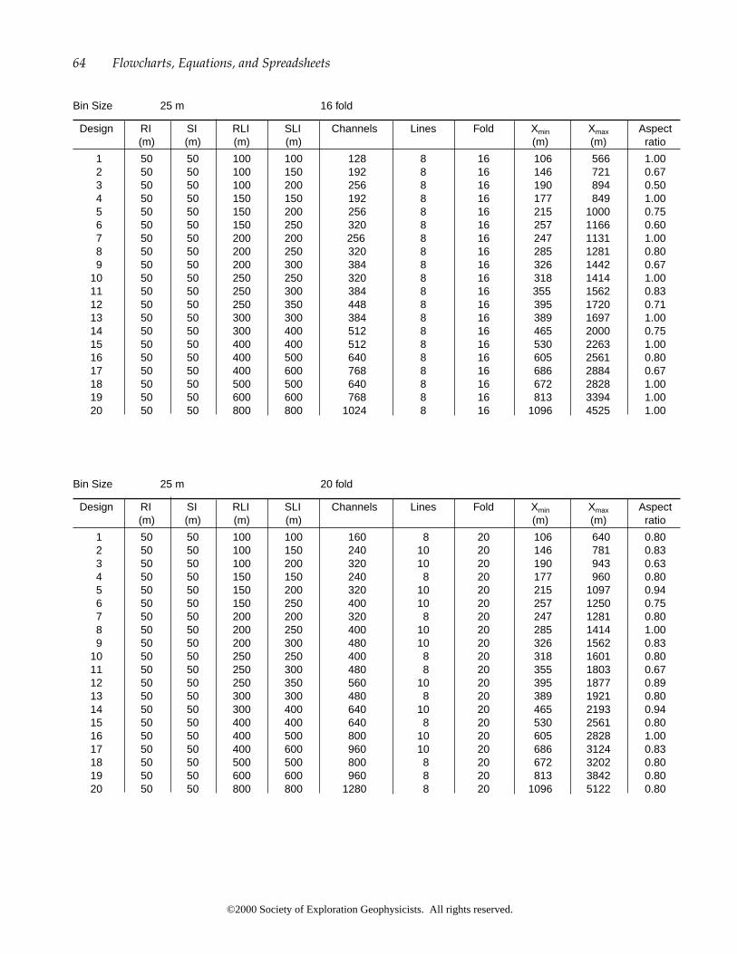
64 Flowcharts, Equations, and Spreadsheets
Bin Size 25 m 16 fold
Design RI SI RLI SLI Channels Lines Fold Xmin Xmax Aspect(m) (m) (m) (m) (m) (m) ratio
1 50 50 100 100 128 8 16 106 566 1.002 50 50 100 150 192 8 16 146 721 0.673 50 50 100 200 256 8 16 190 894 0.504 50 50 150 150 192 8 16 177 849 1.005 50 50 150 200 256 8 16 215 1000 0.756 50 50 150 250 320 8 16 257 1166 0.607 50 50 200 200 256 8 16 247 1131 1.008 50 50 200 250 320 8 16 285 1281 0.809 50 50 200 300 384 8 16 326 1442 0.67
10 50 50 250 250 320 8 16 318 1414 1.0011 50 50 250 300 384 8 16 355 1562 0.8312 50 50 250 350 448 8 16 395 1720 0.7113 50 50 300 300 384 8 16 389 1697 1.0014 50 50 300 400 512 8 16 465 2000 0.7515 50 50 400 400 512 8 16 530 2263 1.0016 50 50 400 500 640 8 16 605 2561 0.8017 50 50 400 600 768 8 16 686 2884 0.6718 50 50 500 500 640 8 16 672 2828 1.0019 50 50 600 600 768 8 16 813 3394 1.0020 50 50 800 800 1024 8 16 1096 4525 1.00
Bin Size 25 m 20 fold
Design RI SI RLI SLI Channels Lines Fold Xmin Xmax Aspect(m) (m) (m) (m) (m) (m) ratio
1 50 50 100 100 160 8 20 106 640 0.802 50 50 100 150 240 10 20 146 781 0.833 50 50 100 200 320 10 20 190 943 0.634 50 50 150 150 240 8 20 177 960 0.805 50 50 150 200 320 10 20 215 1097 0.946 50 50 150 250 400 10 20 257 1250 0.757 50 50 200 200 320 8 20 247 1281 0.808 50 50 200 250 400 10 20 285 1414 1.009 50 50 200 300 480 10 20 326 1562 0.83
10 50 50 250 250 400 8 20 318 1601 0.8011 50 50 250 300 480 8 20 355 1803 0.6712 50 50 250 350 560 10 20 395 1877 0.8913 50 50 300 300 480 8 20 389 1921 0.8014 50 50 300 400 640 10 20 465 2193 0.9415 50 50 400 400 640 8 20 530 2561 0.8016 50 50 400 500 800 10 20 605 2828 1.0017 50 50 400 600 960 10 20 686 3124 0.8318 50 50 500 500 800 8 20 672 3202 0.8019 50 50 600 600 960 8 20 813 3842 0.8020 50 50 800 800 1280 8 20 1096 5122 0.80
©2000 Society of Exploration Geophysicists. All rights reserved.

4.6 Standardized Spreadsheets 65
Bin Size 25 m 24 fold
Design RI SI RLI SLI Channels Lines Fold Xmin Xmax Aspect(m) (m) (m) (m) (m) (m) ratio
1 50 50 100 100 192 8 24 106 721 0.672 50 50 100 150 288 12 24 146 849 1.003 50 50 100 200 384 12 24 190 1000 0.754 50 50 150 150 288 8 24 177 1082 0.675 50 50 150 200 384 8 24 215 1342 0.506 50 50 150 250 480 12 24 257 1345 0.907 50 50 200 200 384 8 24 247 1442 0.678 50 50 200 250 480 8 24 285 1700 0.539 50 50 200 300 576 12 24 326 1697 1.00
10 50 50 250 250 480 8 24 318 1803 0.6711 50 50 250 300 576 8 24 355 2059 0.5612 50 50 250 350 672 8 24 395 2326 0.4813 50 50 300 300 576 8 24 389 2163 0.6714 50 50 300 400 768 8 24 465 2683 0.5015 50 50 400 400 768 8 24 530 2884 0.6716 50 50 400 500 960 8 24 605 3400 0.5317 50 50 400 600 1152 12 24 686 3394 1.0018 50 50 500 500 960 8 24 672 3606 0.6719 50 50 600 600 1152 8 24 813 4327 0.6720 50 50 800 800 1536 8 24 1096 5769 0.67
Bin Size 25 m 30 fold
Design RI SI RLI SLI Channels Lines Fold Xmin Xmax Aspect(m) (m) (m) (m) (m) (m) ratio
1 50 50 100 100 240 10 30 106 781 0.832 50 50 100 150 360 12 30 146 960 0.803 50 50 100 200 480 12 30 190 1166 0.604 50 50 150 150 360 10 30 177 1172 0.835 50 50 150 200 480 12 30 215 1345 0.906 50 50 150 250 600 12 30 257 1540 0.727 50 50 200 200 480 10 30 247 1562 0.838 50 50 200 250 600 12 30 285 1733 0.969 50 50 200 300 720 12 30 326 1921 0.80
10 50 50 250 250 600 10 30 318 1953 0.8311 50 50 250 300 720 12 30 355 2121 1.0012 50 50 250 350 840 12 30 395 2305 0.8613 50 50 300 300 720 10 30 389 2343 0.8314 50 50 300 400 960 12 30 465 2691 0.9015 50 50 400 400 960 10 30 530 3124 0.8316 50 50 400 500 1200 12 30 605 3466 0.9617 50 50 400 600 1440 12 30 686 3842 0.8018 50 50 500 500 1200 10 30 672 3905 0.8319 50 50 600 600 1440 10 30 813 4686 0.8320 50 50 800 800 1920 10 30 1096 6248 0.83
©2000 Society of Exploration Geophysicists. All rights reserved.

66 Flowcharts, Equations, and Spreadsheets
Bin Size 25 m 40 fold
Design RI SI RLI SLI Channels Lines Fold Xmin Xmax Aspect(m) (m) (m) (m) (m) (m) ratio
1 50 50 100 100 320 10 40 106 943 0.632 50 50 100 150 480 10 40 146 1300 0.423 50 50 100 200 640 16 40 190 1281 0.804 50 50 150 150 480 10 40 177 1415 0.635 50 50 150 200 640 10 40 215 1767 0.476 50 50 150 250 800 16 40 257 1733 0.967 50 50 200 200 640 10 40 247 1887 0.638 50 50 200 250 800 10 40 285 2236 0.509 50 50 200 300 960 10 40 326 2600 0.42
10 50 50 250 250 800 10 40 318 2358 0.6311 50 50 250 300 960 10 40 355 2706 0.5212 50 50 250 350 1120 10 40 395 3066 0.4513 50 50 300 300 960 10 40 389 2830 0.6314 50 50 300 400 1280 10 40 465 3534 0.4715 50 50 400 400 1280 10 40 530 3774 0.6316 50 50 400 500 1600 10 40 605 4472 0.5017 50 50 400 600 1920 10 40 686 5200 0.4218 50 50 500 500 1600 10 40 672 4717 0.6319 50 50 600 600 1920 10 40 813 5660 0.6320 50 50 800 800 2560 10 40 1096 7547 0.63
Bin Size 110 ft 12 fold
Design RI SI RLI SLI Channels Lines Fold Xmin Xmax Aspect(ft) (ft) (ft) (ft) (ft) (ft) ratio
1 220 220 440 440 96 6 12 467 2200 0.752 220 220 440 660 144 8 12 641 2649 0.893 220 220 440 880 192 8 12 838 3173 0.674 220 220 660 660 144 6 12 778 3300 0.755 220 220 660 880 192 8 12 946 3734 1.006 220 220 660 1100 240 8 12 1133 4226 0.807 220 220 880 880 192 6 12 1089 4400 0.758 220 220 880 1100 240 6 12 1254 5131 0.609 220 220 880 1320 288 8 12 1434 5298 0.56
10 220 220 1100 1100 240 6 12 1400 5500 0.7511 220 220 1100 1320 288 6 12 1563 6226 0.6312 220 220 1100 1540 336 8 12 1739 6380 0.9513 220 220 1320 1320 288 6 12 1711 6600 0.7514 220 220 1320 1760 384 8 12 2046 7467 1.0015 220 220 1760 1760 384 6 12 2333 8800 0.7516 220 220 1760 2200 480 6 12 2663 10262 0.6017 220 220 1760 2640 576 8 12 3020 10597 0.8918 220 220 2200 2200 480 6 12 2956 11000 0.7519 220 220 2640 2640 576 6 12 3578 13200 0.7520 220 220 3520 3520 768 6 12 4822 17600 0.75
©2000 Society of Exploration Geophysicists. All rights reserved.

4.6 Standardized Spreadsheets 67
Bin Size 110 ft 16 fold
Design RI SI RLI SLI Channels Lines Fold Xmin Xmax Aspect(ft) (ft) (ft) (ft) (ft) (ft) ratio
1 220 220 440 440 128 8 16 467 2489 1.002 220 220 440 660 192 8 16 641 3173 0.673 220 220 440 880 256 8 16 838 3935 0.504 220 220 660 660 192 8 16 778 3734 1.005 220 220 660 880 256 8 16 946 4400 0.756 220 220 660 1100 320 8 16 1133 5131 0.607 220 220 880 880 256 8 16 1089 4978 1.008 220 220 880 1100 320 8 16 1254 5635 0.809 220 220 880 1320 384 8 16 1434 6346 0.67
10 220 220 1100 1100 320 8 16 1400 6223 1.0011 220 220 1100 1320 384 8 16 1563 6873 0.8312 220 220 1100 1540 448 8 16 1739 7570 0.7113 220 220 1320 1320 384 8 16 1711 7467 1.0014 220 220 1320 1760 512 8 16 2046 8800 0.7515 220 220 1760 1760 512 8 16 2333 9956 1.0016 220 220 1760 2200 640 8 16 2663 11269 0.8017 220 220 1760 2640 768 8 16 3020 12692 0.6718 220 220 2200 2200 640 8 16 2956 12445 1.0019 220 220 2640 2640 768 8 16 3578 14934 1.0020 220 220 3520 3520 1024 8 16 4822 19912 1.00
Bin Size 110 ft 20 fold
Design RI SI RLI SLI Channels Lines Fold Xmin Xmax Aspect(ft) (ft) (ft) (ft) (ft) (ft) ratio
1 220 220 440 440 160 8 20 467 2817 0.802 220 220 440 660 240 10 20 641 3437 0.833 220 220 440 880 320 10 20 838 4151 0.634 220 220 660 660 240 8 20 778 4226 0.805 220 220 660 880 320 10 20 946 4825 0.946 220 220 660 1100 400 10 20 1133 5500 0.757 220 220 880 880 320 8 20 1089 5635 0.808 220 220 880 1100 400 10 20 1254 6223 1.009 220 220 880 1320 480 10 20 1434 6873 0.83
10 220 220 1100 1100 400 8 20 1400 7043 0.8011 220 220 1100 1320 480 8 20 1563 7932 0.6712 220 220 1100 1540 560 10 20 1739 8258 0.8913 220 220 1320 1320 480 8 20 1711 8452 0.8014 220 220 1320 1760 640 10 20 2046 9650 0.9415 220 220 1760 1760 640 8 20 2333 11269 0.8016 220 220 1760 2200 800 10 20 2663 12445 1.0017 220 220 1760 2640 960 10 20 3020 13746 0.8318 220 220 2200 2200 800 8 20 2956 14087 0.8019 220 220 2640 2640 960 8 20 3578 16904 0.8020 220 220 3520 3520 1280 8 20 4822 22539 0.80
©2000 Society of Exploration Geophysicists. All rights reserved.

68 Flowcharts, Equations, and Spreadsheets
Bin Size 110 ft 24 fold
Design RI SI RLI SLI Channels Lines Fold Xmin Xmax Aspect(ft) (ft) (ft) (ft) (ft) (ft) ratio
1 220 220 440 440 192 8 24 467 3173 0.672 220 220 440 660 288 12 24 641 3734 1.003 220 220 440 880 384 12 24 838 4400 0.754 220 220 660 660 288 8 24 778 4759 0.675 220 220 660 880 384 8 24 946 5903 0.506 220 220 660 1100 480 12 24 1133 5920 0.907 220 220 880 880 384 8 24 1089 6346 0.678 220 220 880 1100 480 8 24 1254 7480 0.539 220 220 880 1320 576 12 24 1434 7467 1.00
10 220 220 1100 1100 480 8 24 1400 7932 0.6711 220 220 1100 1320 576 8 24 1563 9060 0.5612 220 220 1100 1540 672 8 24 1739 10234 0.4813 220 220 1320 1320 576 8 24 1711 9519 0.6714 220 220 1320 1760 768 8 24 2046 11806 0.5015 220 220 1760 1760 768 8 24 2333 12692 0.6716 220 220 1760 2200 960 8 24 2663 14960 0.5317 220 220 1760 2640 1152 12 24 3020 14934 1.0018 220 220 2200 2200 960 8 24 2956 15864 0.6719 220 220 2640 2640 1152 8 24 3578 19037 0.6720 220 220 3520 3520 1536 8 24 4822 25383 0.67
Bin Size 110 ft 30 fold
Design RI SI RLI SLI Channels Lines Fold Xmin Xmax Aspect(ft) (ft) (ft) (ft) (ft) (ft) ratio
1 220 220 440 440 240 10 30 622 3213 0.782 220 220 440 660 360 12 30 793 4004 0.763 220 220 440 880 480 12 30 984 4925 0.564 220 220 660 660 360 10 30 933 4862 0.775 220 220 660 880 480 12 30 1100 5620 0.856 220 220 660 1100 600 12 30 1283 6498 0.677 220 220 880 880 480 10 30 1245 6512 0.778 220 220 880 1100 600 12 30 1409 7244 0.909 220 220 880 1320 720 12 30 1586 8096 0.75
10 220 220 1100 1100 600 10 30 1556 8162 0.7611 220 220 1100 1320 720 12 30 1718 8873 0.9312 220 220 1100 1540 840 12 30 1893 9706 0.8013 220 220 1320 1320 720 10 30 1867 9812 0.7614 220 220 1320 1760 960 12 30 2046 11839 0.9015 220 220 1760 1760 960 10 30 2333 13746 0.8316 220 220 1760 2200 1200 12 30 2663 15248 0.9617 220 220 1760 2640 1440 12 30 3020 16904 0.8018 220 220 2200 2200 1200 10 30 2956 17183 0.8319 220 220 2640 2640 1440 10 30 3578 20619 0.8320 220 220 3520 3520 1920 10 30 4822 27492 0.83
©2000 Society of Exploration Geophysicists. All rights reserved.
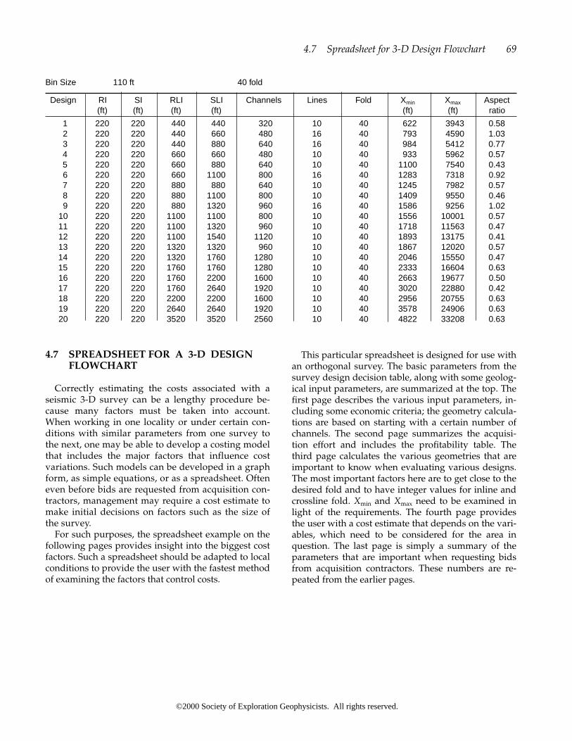
4.7 SPREADSHEET FOR A 3-D DESIGNFLOWCHART
Correctly estimating the costs associated with aseismic 3-D survey can be a lengthy procedure be-cause many factors must be taken into account.When working in one locality or under certain con-ditions with similar parameters from one survey tothe next, one may be able to develop a costing modelthat includes the major factors that influence costvariations. Such models can be developed in a graphform, as simple equations, or as a spreadsheet. Ofteneven before bids are requested from acquisition con-tractors, management may require a cost estimate tomake initial decisions on factors such as the size ofthe survey.
For such purposes, the spreadsheet example on thefollowing pages provides insight into the biggest costfactors. Such a spreadsheet should be adapted to localconditions to provide the user with the fastest methodof examining the factors that control costs.
4.7 Spreadsheet for 3-D Design Flowchart 69
Bin Size 110 ft 40 fold
Design RI SI RLI SLI Channels Lines Fold Xmin Xmax Aspect(ft) (ft) (ft) (ft) (ft) (ft) ratio
1 220 220 440 440 320 10 40 622 3943 0.582 220 220 440 660 480 16 40 793 4590 1.033 220 220 440 880 640 16 40 984 5412 0.774 220 220 660 660 480 10 40 933 5962 0.575 220 220 660 880 640 10 40 1100 7540 0.436 220 220 660 1100 800 16 40 1283 7318 0.927 220 220 880 880 640 10 40 1245 7982 0.578 220 220 880 1100 800 10 40 1409 9550 0.469 220 220 880 1320 960 16 40 1586 9256 1.02
10 220 220 1100 1100 800 10 40 1556 10001 0.5711 220 220 1100 1320 960 10 40 1718 11563 0.4712 220 220 1100 1540 1120 10 40 1893 13175 0.4113 220 220 1320 1320 960 10 40 1867 12020 0.5714 220 220 1320 1760 1280 10 40 2046 15550 0.4715 220 220 1760 1760 1280 10 40 2333 16604 0.6316 220 220 1760 2200 1600 10 40 2663 19677 0.5017 220 220 1760 2640 1920 10 40 3020 22880 0.4218 220 220 2200 2200 1600 10 40 2956 20755 0.6319 220 220 2640 2640 1920 10 40 3578 24906 0.6320 220 220 3520 3520 2560 10 40 4822 33208 0.63
This particular spreadsheet is designed for use withan orthogonal survey. The basic parameters from thesurvey design decision table, along with some geolog-ical input parameters, are summarized at the top. Thefirst page describes the various input parameters, in-cluding some economic criteria; the geometry calcula-tions are based on starting with a certain number ofchannels. The second page summarizes the acquisi-tion effort and includes the profitability table. Thethird page calculates the various geometries that areimportant to know when evaluating various designs.The most important factors here are to get close to thedesired fold and to have integer values for inline andcrossline fold. Xmin and Xmax need to be examined inlight of the requirements. The fourth page providesthe user with a cost estimate that depends on the vari-ables, which need to be considered for the area inquestion. The last page is simply a summary of theparameters that are important when requesting bidsfrom acquisition contractors. These numbers are re-peated from the earlier pages.
©2000 Society of Exploration Geophysicists. All rights reserved.

Project: SEG 3-D Client: ABC Oil Company
Location: TEXAS GEDCO file #:
9/1/99
PROSPECT INFORMATIONUNITS units M M (metric) or I (imperial)
fold of good 2-D data 20 at 10 m trace spacingDIP steepest dips 5.0 degrees WSWSM mute for shallow markers needed
for isochroning 600 mDEPTH target depth 1900 mTWT target two-way time 1.4 sBASE basement depth 2500 mVint Vint immediately above the target
horizon 3000 m/sfdom fdom at the target horizon 40 Hzfmax fmax at the target horizon 70 Hz
lateral target size 200 marea to be fully imaged 80 km2
layout method orthogonal
fold 20 30bin size 25 m 25 mXmin 600 m 361 mXmax 2000 m 2052 mtotal migration apron range 754 m to 1697 m
INPUTshape rectanglereceiver line direction EWsource line direction NS
RI receiver interval 50 mSI source interval 50 mPBr processing bin in receiver direction 25 mPBs processing bin in source direction 25 mRLI receiver line interval 200 m affects cross-line offset and patch sizeSLI source line interval 300 m affects in-line fold, foldLRL length of receiver lines 8.000 kmLSL length of source lines 10.000 kmNC number of channels 720 affects fold, patch size try 720 channelsLINES/REC patch 12 � 60
receiver array 9 over 5 m circlesource array 1 over 50 m
IROLL roll on/off stations YesX ROLL roll on/off lines YesSWATH swath width (max � NRL/2) 3 check for fold stripingDROP number of consecutive shots which 5 out of 80 for access reasons only—not on adjoining
may be dropped source lines except along the edges of the surveyX OFFSET1 min. distance of any shot from edge
of patch 800 mNOCUT % of lines not needing line cuts 30 % should total 100%CUT % of existing cut lines 25 % should total 100%CATCUT % of cat cut lines 10 % should total 100%HAND % of hand-cut lines 35 % should total 100%CROP % of line km on farm land with crop 20 %
% of acceptable dead traces 2.0 %SHOT/DAY estimated shotpoints per day 250
calculateddesired
70 Flowcharts, Equations, and Spreadsheets
�
©2000 Society of Exploration Geophysicists. All rights reserved.

Project: SEG 3-D Client: ABC Oil Company
Location: TEXAS GEDCO file #:
9/1/99
SOURCE PARAMETERSdynamite
HOLES number of holes 3HOLEDEPTH hole depth 15 mCHARGE charge size per hole 1 kg
vibroseisnumber of vibrators 4number of sweeps 8sweep length 12 spad time 96 ssweep frequency—start 10 Hzsweep frequency - end 90 Hzsweep rate 6.7 Hz/ssweep type 3 dB/octavesource interval 50 mmax move-up for each sweep 6.25 m
other sourcesUTM coordinatesX of SW cornerX of NE cornerY of SW cornerY of NE cornercentral meridianin-line angle - rec.
PROFITABILITY TABLE without 3-D with 3-D 0% changePsource probability of source 90% 90% 0%Pmigration probability of migration/hydrocarbons 80% 80% 0%Preservoir probability of reservoir/porosity 70% 80% 14%Ptrap probability of seal/trap 30% 40% 33%NPVsuccess net present value of successful well $8,000,000 $8,000,000NPVfailure net present value of dry well ($1,500,000) ($1,500,000)Pes probability of economic success 15% 23% 52%Pef probability of economic failure 85% 77% 9%EMV expected monetary value ($63,600) $688,800
VOI Value of Information (e.g., 2-D, 3-D, interpretations) ($752,400)
Required success ratio for single well 16% 22% 39%
4.7 Spreadsheet for 3-D Design Flowchart 71
©2000 Society of Exploration Geophysicists. All rights reserved.

Project: SEG 3-D Client: ABC Oil Company
Location: TEXAS GEDCO file #:
9/1/99
CALCULATEDNBR/S natural bin dimensions 25 � 25 mSBR/S sub-bin dimensions 25 � 25 m
RLI/SI 4.00SLI/RI 6.00
NBINS number of processing bins 128000NTRACE number of recorded traces 4003920
full fold at offset sub-binIFOLD in-line fold 5.0 5.0 5.0XFOLD cross-line fold 6.0 6.0 6.0FOLD total fold 30.0 30.0 30.0
desired 3-D fold according to Krey 23.2maximum fold assuming all
receivers live 1333IROLLS in-line rolls 26XROLLS cross-line rolls 15ROLLS total number of rolls 431
in-line templates 27cross-line templates 16
TEMPLATES total number of template positions 432Vave average velocity to the target zone 2714 m/sFZ Fresnel zone radius before migration 254 mDIFF apron to capture � 95% of
diffraction energy 1097 mMA migration aperture 166 mTAPER fold taper @ 20% of target depth 380 mITAPER TAPER-in-line 600 mXTAPER TAPER-cross-line 500 m
fold rate - in-line 15 per SLIfold rate - cross-line 12 per RLIperiodicity - in-line 0 bins or 0.0 source linesperiodicity - cross-line 24 bins or 3.0 receiver lines
TMA total migration aperture range 754 m to 1697 m
72 Flowcharts, Equations, and Spreadsheets
©2000 Society of Exploration Geophysicists. All rights reserved.

Fal aliasing frequency before migration 344 HzFalm aliasing frequency after migration 343 HzLRES lateral resolution 38 m bin size should be smaller than thisVRES vertical resolution 38 mkNr Nyquist wavenumber
(receiver direction) 0.800 1/mapparent velocites smaller than 88 m/s will be suppressed by receiver array
kNs Nyquist wavenumber (source direction) 0.000 1/m
apparent velocites smaller than 0 m/s no source arraySIZE size of survey 80.0 km2
NETSIZE size of survey net of total migration taper as 20% of depth plus Fresnel zoneaperture 58.4 km2
TNRL number of receiver lines 51.0 try 10.000 km for source line lengthTNSL number of source lines 27.7 try 8.100 km for receiver line lengthTRL total length— receiver lines 408.0 kmTSL total length—source lines 276.7 km
number of receivers per receiver line 161.0NREC number of receiver points 8211NSHOTS number of source points 5561NR number of receiver stations
per square km 100 /km2
NS number of source points per square km 67 /km2
IPATCH in-line patch size 3000 mXPATCH cross-line patch size including swath 2800 m
cross-line patch excluding swath 2400 mA aspect ratio including swath 0.93
aspect ratio excluding swath 0.80IOFFSET in-line offset 1475 mXOFFSET cross-line offset 800 m to 1400 mXmin straight largest min offset 361 mXmin straight largest min offset—one bin offset 326 mXmax largest max offset recorded 2052 m ***Xmax is larger than the necessaryXmax
DAYS acquisition days 22.2 days
4.7 Spreadsheet for 3-D Design Flowchart 73
©2000 Society of Exploration Geophysicists. All rights reserved.

Project: SEG 3-D Client: ABC Oil Company
Location: TEXAS GEDCO file #:
9/1/99
COSTSmin average max
government approvals $2,000 $2,000permit agent $500 /day $22,000permitting $0 /km2 $0 $4,000 $7,000 $10,000 /sectionreceiver line permits $400 /km $163,200 $300 $400 $500 /misource line permits $800 /km $221,333 $800 $1,200 $1,600 /migeneral damages $100 /km $68,467 $100 $200 $300 /kmcrop damages $750 /ha $79,786 $200 $300 $3,000 /acretimber salvage $150 /ha $3,617 $40 $150 $154 /hascouting $550 /day $12,100 $525 $588 $650 /dayadvance man $550 /day $24,200 $525 $588 $650 /daycat push $550 /day $24,200 $500 $575 $650 /daysurvey crew-perimeter $900 /day $19,800 $875 $913 $950 /daybird dog $550 /day $12,110 $500 $575 $650 /dayhealth and safety management $550 /day $12,110 $500 $575 $650 /dayline cutting-open existing $600 /km 171.2 $102,700 $300 $650 $1,000 /kmline cutting-cat $1,000 /km 68.5 $68,467 $500 $1,000 $1,500 /kmline cutting-hand $1,500 /km 239.6 $359,450 $500 $1,750 $3,000 /kmdrilling $0.30 /ft $246,241 $0.45 $0.85 $1.25 /ftmob/demob $0 $0 $2,000 $3,000 $4,000 eachacquisition $0 /shot $0 $145 $273 $400 /shotacquisition $15,000 /km2 $1,200,000 $8,000 $11,500 $15,000 /km2
test holes $100 for 8 $800 $80 $140 $200 /holeclean-up $150 /km $102,700 $0 $350 $700 /kmsurvey calculations $21 /km $23,134 $21 $21 $21 /kmprocessing $20 /shot $111,220 $15 $19 $23 /shot3-D design charge, min. $925 /survey $925 /surveyproject management,
min. estimate $600 /day $26,693 /dayFlexi-Bin license fee $300 /km2 /km2
interpretation $700 /day $93,425 /dayworkstation rental $840 /day $74,740 /dayreproduction $700 $700 $400 $700 $1,000contingency 10% $307,610TOTAL COST $3,383,706
cost per section $109,541/mi2 $150,096/mi2
cost per km2 $42,296/km2 $57,955/km2
cost per recorded trace $0.85
Please note that all numbers are estimates only!!
prepared by: Andreas Cordsen, P. Geoph.Geophysical Exploration & Development Corporation#1200, 815-8th Avenue SWCalgary, Alberta, Canada T2P 3P2(403) 262-5780 fax (403) 262-8632email: [email protected] last update: 22-Apr-99 version 3.0
net of halo
74 Flowcharts, Equations, and Spreadsheets
©2000 Society of Exploration Geophysicists. All rights reserved.

Project: SEG 3-D FOR BID REQUEST
Location: TEXAS GEDCO file #: 1999
9/1/99
PROSPECT INFORMATIONUnits M M (metric) or I (imperial)INPUTshape rectanglereceiver EWsource line direction NSreceiver interval 50 msource interval 50 mprocessing bin in receiver direction 25 mprocessing bin in source direction 25 mreceiver line interval 200 msource line interval 300 mnumber of receiver points 8211number of source points 5561length of receiver lines 8.000 kmlength of source lines 10.00 kmnumber of channels 720patch 12 � 60receiver array 9 over 5 m circlesource array 1 over 50 mroll on/off stations yesswath width (max � NRL/2) 3number of consecutive shots which may be dropped 5 out of 80 for access reasons only—not on
adjacent source linesmin. distance of any shot from edge of patch 800 m except along the edges of the survey% of lines not needing line cuts 30 % should total 100%% of existing cut lines 25 % should total 100%% of cat cut lines 10 % should total 100%% of hand-cut lines 35 % should total 100%$ of line km on farm land with crop 20 %% of acceptable dead traces 2 %
dynamitenumber of holes 3hole depth 15 mcharge size per hold 1 kg
vibroseisnumber of vibrators 4number of sweeps 8sweep length 12 spad time 96 ssweep frequency -start 10 Hzsweep frequency-end 90 Hzsweep rate 6.67 Hz/ssweep type 3 dB/octavesource interval 50 mmax move-up for each sweep 6.25 m
4.7 Spreadsheet for 3-D Design Flowchart 75
�
©2000 Society of Exploration Geophysicists. All rights reserved.

4.8 COST MODEL
The equation,
(4.12)
is the essence of a cost model developed by Caltex Pa-cific Indonesia (CPI). This model normalizes the costof 3-D surveys with the number of recorded mid-points per unit area (Bee et al., 1994). Acquisition costsappear to have a direct relationship with data density,and one can easily determine a normalized value fordata density using
(4.13)
Example:
or
and
Cost per midpoint �$20 000
40 000� $0.50/midpoint.
25 � 27.88 � 106
82.52� 102 400 midpoints/mi2,
Data Density �25 � 106
252� 40 000 midpoints/km2,
Fold � U
B2 or Fold � U
Bs � Br
.
3-D Data Density �
SD � NC �Fold
B2,
If the survey cost is $20 000/km2 ($51 200/mi2) forfull-fold coverage, the cost per midpoint is $0.50.Making comparative calculations for the cost per mid-point of 2-D data may convince management of thecost advantage of a 3-D survey. Assuming a group in-terval of 20 m (55 ft), 30 fold, and a cost of $6000/km($11 520/mi) for 2-D data, then
(4.14)
or � 5760 midpoints/mi
and
or
The typical 2-D comparative cost is $2/midpoint inthe above example, which is four times the 3-D cost of$0.50/midpoint. Although the 3-D cost is lower on aper-midpoint basis, one must ask whether the addi-tional cost of 3-D coverage is warranted or whether ahigher resolution 2-D data set would suffice.
$11 520
5 760 midpoints� $2/midpoint for 2-D.
Cost per midpoint �$6000
$3000� $2/midpoint for 2-D,
�30 � 1000
10� 3000 midpoints/km,
2-D Data Density �Fold � U
CDP Spacing
76 Flowcharts, Equations, and Spreadsheets
©2000 Society of Exploration Geophysicists. All rights reserved.

Numerous layout strategies have been developedfor 3-D surveys. One has to establish which featuresare important in the area of the survey in order to se-lect the best design option. A start at such evaluationis possible with the series of displays that have beenprepared for each design strategy in this chapter. Alldesigns in this chapter are based on a recording patchof 12 lines with 60 stations per line. The aspect ratio isgenerally close to 0.8. Each design will be describedusing the following sequence of displays:
a) Layout—full scale,b) Layout—zoomed,c) Xmin distribution,d) Offset distribution within each bin,e) Offset distribution in parallel rows of bins
(within a box),f ) Azimuth distribution within each bin.
For improved comparisons, all Xmin distributionsare scaled similarly. Line spacings are comparable aswell, with any exceptions noted.
5.1 FULL-FOLD 3-D
A full-fold 3-D survey is one where source pointsand receiver stations are distributed on an even two-dimensional grid (Figures 5.1a, 5.1b) with stationspacings equal to line spacings. The grids are offset byone bin size. A full-fold 3-D survey has outstandingoffset and azimuth distributions as illustrated in Fig-ures 5.1c–5.1f, as long as one can afford to recordwith a large number of channels. All other 3-D de-signs are basically subsets of such full-fold surveys,and the designer has to decide which aspects of a 3-Ddesign are absolutely necessary and which can becompromised.
5.2 SAMPLING THE 5-D PRESTACKWAVEFIELD
The ideal survey samples the 5-D prestack wavefieldW(t, xs , ys , xr , yr) that is dependent upon traveltime tand the source and receiver locations, i.e., xs , ys , xr , yr
(Vermeer, 1998a.) Three-dimensional surveys generallyrecord only a portion of this 5-D wavefield with linespacings that are greater than the station spacings.From the under-sampled 5-D wavefield that has beenacquired, one can form many different 3-D subsetssuch as common source and receiver gathers, cross-spreads, etc. Some of the different 3-D subsets can bevisualized from Figure 5.2. The trace at midpoint M is amember of the common-source gather (horizontalline), the common-receiver gather (vertical line), thecommon-azimuth gather (diagonal line), and the com-mon-offset gather (circle); after Vermeer, 1998a.
Vermeer (1998a) discussed the concept of “symmet-ric sampling.” The basic idea of this theory can best beexplained by the statement, “Make common-receivergathers look like common-shot gathers.” This philoso-phy leads to the criteria:
shot interval � receiver interval (SI � RI),shot line interval � receiver line interval (SLI �
RLI), maximum in-line offset � maximum cross-line off-set,center-spread acquisition for shots and receivers,andshot arrays required as much as receiver arrays.
Application of these criteria to orthogonal geometryleads to square cross-spreads. Note that a conven-tional orthogonal geometry acquired with a square re-ceiver patch can be decomposed into a series of over-lapping square cross-spreads.
77
5Field Layouts
©2000 Society of Exploration Geophysicists. All rights reserved.

78 Field Layouts
Fig. 5.1. Full-fold 3-D survey; a. layout—full scale, b. layout—zoomed, c. Xmin distribution, d. offset distribution withineach bin, e. offset distribution in parallel rows of bins (within a box), f. azimuth distribution within each bin.
©2000 Society of Exploration Geophysicists. All rights reserved.
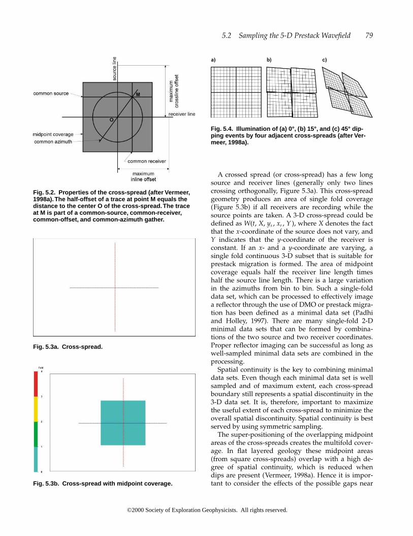
A crossed spread (or cross-spread) has a few longsource and receiver lines (generally only two linescrossing orthogonally, Figure 5.3a). This cross-spreadgeometry produces an area of single fold coverage(Figure 5.3b) if all receivers are recording while thesource points are taken. A 3-D cross-spread could bedefined as W(t, X, ys , xr , Y ), where X denotes the factthat the x-coordinate of the source does not vary, andY indicates that the y-coordinate of the receiver isconstant. If an x- and a y-coordinate are varying, asingle fold continuous 3-D subset that is suitable forprestack migration is formed. The area of midpointcoverage equals half the receiver line length timeshalf the source line length. There is a large variationin the azimuths from bin to bin. Such a single-folddata set, which can be processed to effectively imagea reflector through the use of DMO or prestack migra-tion has been defined as a minimal data set (Padhiand Holley, 1997). There are many single-fold 2-Dminimal data sets that can be formed by combina-tions of the two source and two receiver coordinates.Proper reflector imaging can be successful as long aswell-sampled minimal data sets are combined in theprocessing.
Spatial continuity is the key to combining minimaldata sets. Even though each minimal data set is wellsampled and of maximum extent, each cross-spreadboundary still represents a spatial discontinuity in the3-D data set. It is, therefore, important to maximizethe useful extent of each cross-spread to minimize theoverall spatial discontinuity. Spatial continuity is bestserved by using symmetric sampling.
The super-positioning of the overlapping midpointareas of the cross-spreads creates the multifold cover-age. In flat layered geology these midpoint areas(from square cross-spreads) overlap with a high de-gree of spatial continuity, which is reduced whendips are present (Vermeer, 1998a). Hence it is impor-tant to consider the effects of the possible gaps near
5.2 Sampling the 5-D Prestack Wavefield 79
Fig. 5.2. Properties of the cross-spread (after Vermeer,1998a).The half-offset of a trace at point M equals thedistance to the center O of the cross-spread.The traceat M is part of a common-source, common-receiver,common-offset, and common-azimuth gather.
Fig. 5.3a. Cross-spread.
Fig. 5.3b. Cross-spread with midpoint coverage.
Fig. 5.4. Illumination of (a) 0°, (b) 15°, and (c) 45° dip-ping events by four adjacent cross-spreads (after Ver-meer, 1998a).
©2000 Society of Exploration Geophysicists. All rights reserved.

80 Field Layouts
Fig. 5.5. Swath acquisition method (parallel line concept); a layout—full scale, b. layout—zoomed, c. Xmin distribu-tion, d. offset distribution within each bin, e. offset distribution in parallel rows of bins (within a box), f. azimuth distri-bution within each bin.
©2000 Society of Exploration Geophysicists. All rights reserved.

the edges of the midpoint areas (Figure 5.4). These ef-fects are reduced by increasing the fold and by keep-ing the amount of overlap as large as possible (seeSection 9.5). If, for example, the nominal fold is 30 fora 3-D survey where severe dips are present, then theareas of the gaps in the single-fold cross-spread cov-erage will still have 28 fold where two of such gapsare crossing each other. A 10% fold reduction mightnot be noticeable in this case; however, in a lowerfold survey the reduction percentage is far greaterand therefore the effect would be more severe.
5.3 SWATH
The swath acquisition method was used in the ear-liest 3-D designs (Figures 5.5a, 5.5b). In this geometry,source and receiver lines are parallel and usually coin-cident. While source points are taken on one line, re-ceivers are recording not only along the source linebut also along neighboring parallel receiver lines, cre-ating swath lines halfway between pairs of source andreceiver lines. The Xmin distribution has almost zerovalues on the source lines and values equal to the linespacings on the swath lines (Figure 5.5c). The offsetdistribution in all occupied bin lines is excellent (Fig-ures 5.5d, 5.5e). However, inadequate sampling in thecross-line direction makes this design a “poor man’s3-D,” because many bins are empty. The azimuth mixis very narrow (for few receiver lines) and depends onthe number of live receiver lines in the recordingpatch and the line spacing (Figure 5.5f ). Most com-panies prefer to have the source points at the half-integer positions. Parallel swaths are sometimes considered on land when severe surface restrictionsexist, or when costs have to be minimized. The opera-tional advantages are attractive, but are achieved atthe cost of a poor azimuth mix and poor cross-linesampling.
A gapped in-line technique has been developed tofurther reduce costs in the jungle environment of In-donesia (Bee et al., 1994). Gapped in-line swath shoot-ing does not necessarily use all of the lines of a regu-lar swath geometry as source and/or receiver lines.Swath shoots are also an inherent part of marine 3-Dseismic surveys because of the practical aspect of tow-ing air gun arrays and hydrophone cables behind avessel. In the marine case, however, there are enoughsource lines and receiver lines (streamers) to createcontiguous lines of midpoints (complete coverage).All such designs can be classified as parallel geome-tries that attempt to create continuous common-offsetgathers as a 3-D subset.
5.4 ORTHOGONAL
Generally, source and receiver lines are laid out or-thogonal to each other. Because the receivers cover alarge area, this method is sometimes referred to as thepatch method (Figures 5.6a, 5.6b). This geometry isparticularly easy for the survey crew and recordingcrew, and keeping track of station numbering isstraightforward. In an orthogonal design, the activereceiver lines form a rectangular patch surroundingeach source point location; creating a series of cross-spreads that overlap each other. The patch often has alonger axis in the in-line direction. The in-line offsetsare usually close to the desired offsets that will be in-cluded in the stack. If the cross-line offset within thepatch is close to the maximum offset for stack, thenmost of the receiver line farthest from the source pointwill be useless because much of the data recorded onthat line will be muted in processing. Depending onthe receiver line spacing, the aspect ratio of the axes ofthe patch is usually between 0.6 and 1.0. An aspect ra-tio near 0.85 (see The 85% Rule, Section 3.4) is usuallyacceptable. The source points are assumed to be lo-cated at the center of the patch, although this is not anecessity. When shooting in areas of steep regionaldip, one may want to consider asymmetric patches.Alternating symmetric and then asymmetric patchesare also useful for operational reasons where the sur-vey is at the limit of the available equipment for thecrew. This technique allows more surface area to beacquired prior to receiver station moves.
In the orthogonal method example, receiver linesare oriented east-west and source lines north-south (asshown in Figures 5.6a, 5.6b). This method is easy tolay out in the field and can accommodate extra equip-ment (layout ahead of shooting) and roll-along opera-tion. Usually, all the source points between adjacentreceiver lines are recorded, then the receiver patch isrolled over one (or more) line(s) and the process is re-peated. Figure 5.6c shows the Xmin distribution for theorthogonal design. The Xmin for a particular bin issmallest at the line intersections and increases towardthe center of the boxes. The offset distribution is good(depending on the number of channels in the record-ing patch), but deteriorates towards the center of theboxes where the shorter offsets are missing (Figure5.6d). The offsets in parallel rows of bins show a ten-dency toward distinct patterning for offset limitedstacks (tighter mutes for the shallower section), whichmay result in severe acquisition footprints at shallowlevels (Figure 5.6e). The azimuth distribution for theorthogonal method is uniform as long as a widerecording patch is used (Figure 5.6f).
5.4 Orthogonal 81
©2000 Society of Exploration Geophysicists. All rights reserved.

82 Field Layouts
Fig. 5.6. Orthogonal acquisition method; a. layout—full scale, b. layout—zoomed, c. Xmin distribution, d. offset distrib-ution within each bin, e. offset distribution in parallel rows of bins (within a box), f. azimuth distribution within eachbin.
©2000 Society of Exploration Geophysicists. All rights reserved.

5.5 BRICK
The brick pattern (Figures 5.7a, 5.7b) was devel-oped in an attempt to improve the offset distributionof the orthogonal method. By moving the groups ofsource points that lie between alternate receiver linesto a half-line position, the pattern of offset distribu-tion becomes more random in nature. In practice, it isinteresting to note that a square patch (or a large as-pect ratio) gives rise to more or less the same offsetdistribution for either the orthogonal (Figure 5.6d) orthe brick method (Figure 5.7d). For a narrow azimuthpatch, the offset distribution of a brick pattern is supe-rior to that of an orthogonal design.
If one considers a typical box as defined earlier,then it can be shown that the largest minimum offsetXmin is significantly less than in the orthogonal designassuming the same source and receiver line intervals(Figure 5.7c). Xmin in the brick pattern design dependsupon the line spacings. Because of the staggeredsource lines, there is no easy formula for the value ofXmin or its location; therefore, its distribution shouldbe confirmed with a modeling package. However, thebrick design method allows one to increase the re-ceiver line interval over the orthogonal design with-out increasing Xmin as much as in the orthogonal de-sign. If the source points and receivers are offset at theline intersections, Xmin is slightly smaller (approxi-mately bin) than without the offset.
The offsets in parallel rows of bins show a slightimprovement over the orthogonal design; this may result in less acquisition footprint at shallow levels(Figure 5.7e). The brick design generally offers betterazimuth distribution in addition to an improved off-set distribution for rectangular patches (Figure 5.7f ).Brick patterns are used in areas where permit costsare not an issue and easy access is provided to all lo-cations, such as in the desert. Statics coupling remainsa problem for any regular 3-D geometry except for thefull-fold 3-D because the sources and receivers are un-coupled. The brick design has discontinuous com-mon-receiver gathers because the reflectors are bro-ken due to the bricking of the source points (Vermeer,1998a). This leads to acquisition footprints where lin-ear shot noise is present.
A double brick design refers to a four-line swath(Figure 5.7g). Triple brick refers to a six-line swath(Figure 5.7h), and quadruple brick to an eight-lineswath (Figure 5.7i). In all of these designs, only thecenter line of source points is being recorded. Theserelatively narrow patches offer an improved offsetdistribution over the orthogonal design and even overa square patch of a brick pattern. It follows that one
12
can carry this design concept to a point where allsource point locations fall onto a diagonal rather thanon staggered lines (see Nonorthogonal Geometries,Section 5.6).
Because of the shifting of the source lines in brickdesigns, it is not necessary to have in-line fold andcross-line fold independently as integers (calculatedas per Chapter 2).
The traditional technique of bricking only thesources is widely accepted although one can brick thereceivers instead. In areas of dense cultural interfer-ence, sources can be placed upon the roads andbricked receivers can be used to fill in the brick pat-tern. The technique can also be extended to a brick-brick design, where both the source and receivers arebricked with the advantage of reducing the amount ofline cutting or crop damages per acre of coveragewhen compared to a conventional brick design.
5.6 NONORTHOGONAL
Nonorthogonal (or slanted) arrangements of sourceand receiver lines (Figures 5.8a, 5.8b) are used to getthe benefits of the offset distributions of the brick de-sign without some of the disadvantages, such as 90°turns and noncontinuous source lines (and thereforecommon receiver-gathers). For nonorthogonal de-signs, one needs to be careful when deciding whetherto measure the station interval inline or to stretch it tofall on grid points.
Assuming a station interval of 60 m (220 ft), thesource points in this example should be stretched outby a factor of
or
With this stretch, the bin size of 30 m � 30 m (110 ft� 110 ft) can be maintained, and the midpoints fallinto the center of the bins. Figure 5.8a shows an exam-ple of the nonorthogonal method with a 45° angle be-tween the source lines and the orthogonal to the re-ceiver lines. The source points for each patch lie in thecenter of the patch between two adjacent receiverlines (Figure 5.8b). This basic unit is moved aroundthe survey. This method is often shot with only a fewreceiver lines per patch (narrow azimuth) and is oper-
220 ft
cos 45��
220 ft
0.707� 311 ft.
60 m
cos 45��
60 m
0.707� 85 m
5.6 Nonorthogonal 83
©2000 Society of Exploration Geophysicists. All rights reserved.

84 Field Layouts
Fig. 5.7. Brick acquisition method; a. layout—full scale, b. layout—zoomed, c. Xmin distribution, d. offset distributionwithin each bin, e. offset distribution in parallel rows of bins (within a box), f. azimuth distribution within each bin.
©2000 Society of Exploration Geophysicists. All rights reserved.

5.7 Flex-Bin© or Bin Fractionation 85
ationally attractive because of the straight source andreceiver line layout. With a narrow azimuth patch,fold builds up quickly around the survey edges in thecross-line direction. Figure 5.8c shows the Xmin distrib-ution for one example of the nonorthogonal design.The position of the largest minimum offset (Xmin)changes with the line angle and the line intervals. Oneshould check the Xmin distribution with a softwarepackage. The offset distribution for the 45° angle de-sign is well dispersed with few duplicated offsets(Figures 5.8d and 5.8e). The azimuth distribution isvery good also; however, it depends on the number ofreceiver lines in the patch (Figure 5.8f ).
A special case for the nonorthogonal design is thecase where the relative geometry in the cross-line direc-tion is repeated every second receiver line (Figure5.9a). For this case, the angle between the source linesand the orthogonal to the receiver lines is 26.565° (arctan 0.5) when the line intervals are equal. The sourcepoints in this example should be stretched out by a fac-tor of 60 m � cos 26.565° � 60 m � 0.894 � 72.1 m (or220 ft � cos 26.565° � 220 ft � 0.894 � 246 ft). The se-lection of this angle causes the midpoints to be distrib-uted as indicated in Figure 5.9b. This midpoint distrib-ution is not good for square binning (compare Figure5.8b); however, it is ideal for hexagonal binning (seeSection 5.11). The Xmin distribution appears far worsethan in the previous example of the 45° angle becausethe line spacings are greater. Finally the offset and az-imuth distributions are improved over the 45° anglegeometry (hence less footprint) (Figures 5.9d-5.9f ).
5.7 FLEXI-BIN® OR BIN FRACTIONATION
The Flexi-Bin® method was developed and patentedby GEDCO (Cordsen, 1993a, 1993b, 1995a). In thismethod, source points and receivers can be laid out inmany different ways. Basically, one must ensure thatsource and receiver line spacings are noninteger withrespect to the group interval. In Figure 5.10 for exam-ple, RI � SI � 60 m, RLI � 260 m, and SLI � 320 m.This causes midpoints to fall in a regular pattern in-side each CMP bin (Figure 5.10b). In many othermethods, the theoretical midpoints are at the bin center.
In the above example, (60 m, 60 m, 260 m, 320 m)nine groups of midpoints of 10 m � 10 m size resultin each CMP bin of 30 m � 30 m. In processing, onecan choose to stack these sub-bins or microbins (ninetimes as many as regular bins), thereby achievingfiner midpoint (bin) spacings. With a stack traceevery 10 m instead of every 30 m, these traces have
Fig. 5.7. (continued) Brick acquisition method; g. dou-ble brick layout, h. triple brick layout, i. quadruple bricklayout.
©2000 Society of Exploration Geophysicists. All rights reserved.

86 Field Layouts
Fig. 5.8. Nonorthogonal—45°—arrangement of source and receiver lines; a. layout—full scale, b. layout—zoomed, c.Xmin distribution, d. offset distribution within each bin, e. offset distribution in parallel rows of bins (within a box), f. az-imuth distribution within each bin.
©2000 Society of Exploration Geophysicists. All rights reserved.

5.7 Flex-Bin© or Bin Fractionation 87
Fig. 5.9. Nonorthogonal—26.565°—arrangement; a. layout—full scale, b. layout—zoomed, c. Xmin distribution, d. off-set distribution within each bin, e. offset distribution in parallel rows of bins (within a box), f. azimuth distributionwithin each bin.
©2000 Society of Exploration Geophysicists. All rights reserved.
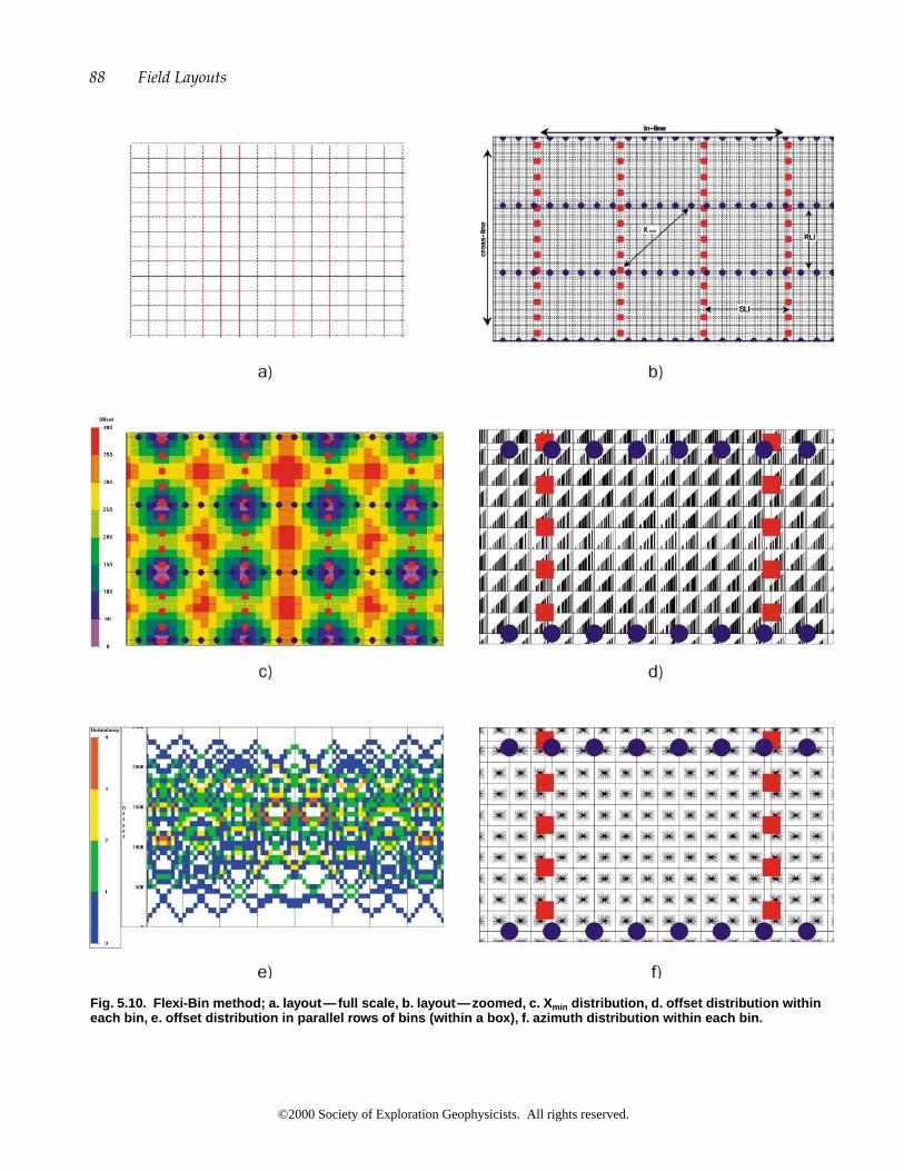
88 Field Layouts
Fig. 5.10. Flexi-Bin method; a. layout—full scale, b. layout—zoomed, c. Xmin distribution, d. offset distribution withineach bin, e. offset distribution in parallel rows of bins (within a box), f. azimuth distribution within each bin.
©2000 Society of Exploration Geophysicists. All rights reserved.

lower fold, and therefore, potentially lower signal-to-noise ratio. On the other hand, one can inprove theS/N by increasing the bin size. This decision can bemade on the basis of data quality after the data arerecorded.
The Xmin distribution is similar to the orthogonallayout (Figure 5.10c). Each normal CMP bin still con-tains as many traces as before, but with a somewhatimproved offset (Figures 5.10d, 5.10e) and azimuthdistribution (Figure 5.10f ). Full statics coupling (seeChapter 10) is a major advantage of this method be-cause of the nonrepeating geometry at neighboringline intersections. The possibility exists that thesmaller stack trace interval may reveal a feature thatone might miss at larger stack trace spacing. There arenumerous operational advantages to the Flexi-Bin®
method, such as easier field operations, excellent stat-ics coupling (Cordsen, 1995b), and other processingflexibilities. In orthogonal shooting, one should con-sider using this noninteger method.
The bin fractionation method (Flentge, 1996) usessource and receiver lines that are staggered by a se-lected fraction of the source station and receiver sta-tion intervals. GRI (1994) describes a survey wherethe fractionation was one-half of the source- and re-ceiver-station intervals. That survey was limited tocreating “quarter cells” in the subsurface. The num-bering of station locations in the field is not parallelfrom line to line; however, this does not create any op-erational problems if reasonable care is exercised.
It has been emphasized (Vermeer, 1997) that anybin fractionation technique merely interleaves two ormore cross-spreads with their sampling intervals cor-responding to the station spacings. Nevertheless thesubsurface samples are distributed on a finer grid ofmidpoints, in particular for subhorizontal events, andmay indeed be beneficial for subsurface definition.Field practice with the Flexi-Bin® method on numer-ous seismic programs has demonstrated some im-provement in lateral interpretability.
5.8 BUTTON PATCH
The button patch method was developed andpatented by ARCO (Bremner et al., 1990) and has rou-tinely been used in many ARCO 3-D surveys. Eachbutton contains a tight pattern of receivers (Figures5.11a, 5.11b), typically 6 � 6, 6 � 8, or 8 � 8. The finalbutton geometry is largely determined by equipmentconsiderations and cable restrictions. There is no re-quirement to keep the receiver patterns square.
Several buttons are combined in a checkerboardpattern to form the receiver patch. Multiple sourcepoints are fired into the receiver patch in a precisemanner. The receiver patch is then rolled to its next lo-cation, while some overlap with the previous patchposition is maintained. Then a similar pattern ofsource points is fired into the new receiver patch. Re-peating source points for different buttons provideimproved statics coupling, while staggered sourcepoints between previous locations offer better mid-point distribution. Frequently, the receiver buttonsand source point locations are distributed irregularlybecause of surface obstructions.
Large channel capacities are necessary to minimizereceiver moves. The shooting trucks, or vibrators,must travel around the patch for each new receiverlayout. If sufficient receivers are available, thenshrewd use of the roll-along switch can eliminate un-necessary movement of the shooters or vibrators. Twoor three patch positions with roll-on can often be cov-ered in one receiver layout.
The receiver buttons are laid out and moved overthe area to be imaged at full-fold. Typically smallerbins with lower fold are used in button patch designsas compared to other design strategies. Source pointsare placed outside this full-fold area to give a fold ta-per around the edges. This geometry achieves longeroffsets without the need to lay out additional equip-ment outside the planned area of the survey. Thistechnique tends to improve migration and DMO be-cause the seismic amplitudes contained on these longoffsets contribute energies to many trace gathers. Be-cause of the discontinuity of common-source gathers,this geometry may have a significant acquisition foot-print.
The button patch method utilizes modern, high-channel systems effectively. High resolution can beachieved by using closer receiver spacing. A smallXmin is present within the receiver buttons (Figure5.11c); however, the Xmin distribution worsens signifi-cantly outside the buttons. Good static coupling re-quires great care at the planning stage. Short-offsetdistribution may be poor, but far-offset distributionshould be good because the source points are outsideof the button patch area (Figure 5.11d). The offsets ina row of bins look good, but display patterning fornear offsets (Figure 5.11e). Some azimuthal bunchingof source-to-receiver raypaths exists because of thebutton layout of the receivers (Figure 5.11f ).
One advantage of this design is that it has the flexi-bility to plan the button holes around obstacles. Thereis also additional flexibility for make-up source points
5.8 Button Patch 89
©2000 Society of Exploration Geophysicists. All rights reserved.

90 Field Layouts
Fig. 5.11. Button patch method; a. layout—full scale, b. layout—zoomed, c. Xmin distribution, d. offset distributionwithin each bin, e. offset distribution in a row of bins (along a receiver line), f. azimuth distribution within each bin.
©2000 Society of Exploration Geophysicists. All rights reserved.

and for compensating for dropped source points. Themajor constraint on the efficiency of the button patchdesign is the requirement for the shooters or vibratorsto move about the survey easily. In some surveys, lim-ited access may make this strategy a poor choice.
5.9 ZIG-ZAG
The zig-zag pattern (Figure 5.12a) is popular indesert areas, or other locations where one has goodaccess between receiver lines. Single source lines arelocated between adjacent pairs of receiver lines for asingle zig-zag (Figure 5.12b). The source point posi-tions should be located on a grid to create centralmidpoints. For 60 m (220 ft) station intervals, and a45° angle between the receiver lines and the sourceline diagonal, the distance between stations on the di-agonal is 85 m (311 ft). In a mirrored zig-zag, everysecond source line is flipped to its mirror image (Fig-ure 5.13a, 5.13b). The offset distribution can be im-proved further by shooting the 3-D grid in a doublezig-zag pattern, as shown in Figures 5.14a and 5.14bwith two sets of vibrators.
For the zig-zag, mirrored, or double zig-zag, thelargest minimum offset Xmin is usually found near thecenter of the open area left by the zig-zag source lines(Figures 5.12c, 5.13c, 5.14c). It is recommended thelargest Xmin be checked using a modeling program.Zig-zag designs are often considered for narrow az-imuth surveys that require good offset distribution.The offset distributions for the single (Figure 5.12d)and mirrored zig-zag designs (Figure 5.13d) are good(using a wide patch); for the double zig-zag design itis outstanding (Figure 5.14d). Figures 5.12e, 5.13e, and5.14e indicate that there is a stronger possibility of ac-quisition footprint with the single zig-zag designsthan with a double zig-zag. Note, however, that thesource effort is increased by a factor of two for thedouble zig-zag. The azimuth distributions are accept-able for a wide-azimuth patch (Figures 5.12f, 5.13f,5.14f ).
The advantages of a zig-zag design are in efficiencyof movement with the vibrator source along very longsource lines; vibrators do not have to cross receiverlines. When compared to a brick or orthogonal de-sign, the zig-zag has minimal moveup time betweensource points and effectively no drive around time.This is particularly true when two vibrator sourcesare used on a zig-zag design compared to a doublebrick. The disadvantage of the zig-zag design is that,if improperly designed, a strong acquisition footprintcan be impressed upon the data.
5.10 MEGA-BIN
This term was coined by PanCanadian for a 3-D de-sign method developed by Goodway and Ragan(1995). The geometry is based on several concepts thatare brought together in a unique way. Any asymmetrybetween the station and line dimensions of conven-tional designs aliases nonrandom, source-generatedsurface noise. The redistribution of the source and re-ceiver locations in the mega-bin design (Figures 5.15a,5.15b) reduces this asymmetry and samples such noisebetter. In addition, the acquisition footprint, which istypical for wide line spacings, is significantly reduced.
Signal-to-noise ratio improves with fold. Withmega-bin, the statistics improve for one row of high-fold bins (and hence higher S/N ratio), while bins inthe neighboring row have zero fold, i.e., these bins areempty (Figure 5.15c). These latter bins are filledthrough premigration f-x interpolation from thehigher fold bins. The f-x interpolation makes this tech-nique different from the earlier swath surveys (seeSection 5.3). The basic geometry of these two meth-ods, however, is comparable; the line spacing in theswath survey was never set to any particular interval,while in the mega-bin technique the line spacing isgenerally four times the bin spacing.
The Xmin distribution has almost zero values on thesource lines and values equal to the line spacings onthe swath lines (Figure 5.15c). The offset distributionon all bin lines is excellent (Figure 5.15d). No othermethod (other than full-fold or swath) covers all off-sets in the occupied rows of bins as well as mega-bin(Figure 5.15e); however, only every other bin is occu-pied. The azimuth distribution is also excellent on theacquisition lines as well as on the intermediate lines(Figure 5.15f ).
The data quality of mega-bin surveys has beenproven to be high in relatively unstructured areas,and independently processed decimation experimentswith an over-sampled 3-D survey (shots and receiverson a 70 m � 70 m grid) have shown this method to beviable. One major advantage of this method is, de-pending on the design, that the source points areplaced along the receiver lines, thereby reducing theline cutting. However, the receiver lines are placedmuch closer together than in an orthogonal geometry.
5.11 HEXAGONAL BINNING
If the midpoints fall into a hexagonal pattern, the midpoints can be binned hexagonally. Thismethod requires 13.4% fewer subsurface samples
5.11 Hexagonal Binning 91
©2000 Society of Exploration Geophysicists. All rights reserved.

92 Field Layouts
Fig. 5.12. Zig-zag method; a. layout—full scale, b. layout—zoomed, c. Xmin distribution, d. offset distribution withineach bin, e. offset distribution in parallel rows of bins (within a box), f. azimuth distribution within each bin.
©2000 Society of Exploration Geophysicists. All rights reserved.
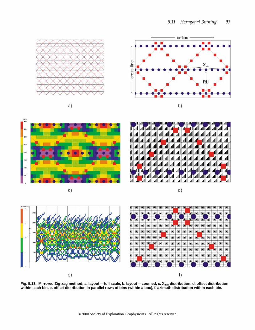
5.11 Hexagonal Binning 93
Fig. 5.13. Mirrored Zig-zag method; a. layout—full scale, b. layout—zoomed, c. Xmin distribution, d. offset distributionwithin each bin, e. offset distribution in parallel rows of bins (within a box), f. azimuth distribution within each bin.
©2000 Society of Exploration Geophysicists. All rights reserved.

94 Field Layouts
Fig. 5.14. Double Zig-zag method; a. layout—full scale, b. layout—zoomed, c. Xmin distribution, d. offset distributionwithin each bin, e. offset distribution in parallel rows of bins (within a box), f. azimuth distribution within each bin.
©2000 Society of Exploration Geophysicists. All rights reserved.

5.11 Hexagonal Binning 95
Fig. 5.15. Mega-bin method; a. layout—full scale, b. layout—zoomed, c. Xmin distribution, d. offset distribution withineach bin, e. offset distribution in parallel rows of bins (within a box), f. azimuth distribution within each bin.
©2000 Society of Exploration Geophysicists. All rights reserved.

in one direction compared to a square grid of mid-points, thereby reducing the acquisition and process-ing effort of the 3-D survey (Bardan, 1997). Either thesource or the receiver effort can be reduced by 13.4%and yet still achieve the same resolution. Hexagonalsampling can be accomplished by many different lay-out methods, one of which was decribed earlier (seeFigure 5.9b).
5.12 STAR
Star shooting involves laying out receiver lines inan arrangement resembling the spokes of a wheel(Figures 5.16a, 5.16b). Source points are taken alongthose same lines. In such surveys one can often haveall receivers live while acquiring the source points.Fold is very high near the center and drops offquickly towards the edges of the survey. A method ofimproving the areal coverage is to offset the lines attheir intersections. The Xmin , offset, and azimuth dis-tributions deteriorate very quickly away from the cen-ter (Figures 5.16c–5.16f).
The field effort for a star survey is very low com-pared to other designs since the star survey is essen-tially a series of crossing 2-D lines. Because of the highfold, many source points near the center of the surveyprobably can be eliminated depending on shallowhorizon requirements. This method has been usedwith considerable success for small structures wheredata showed high S/N content. The method has beenadvocated for salt-domes (or reefs), where this geome-try favors the collection of energy that reflects from allsides of the salt-dome, and long offsets are requiredfor migration purposes. In practice, however, the loca-tion of the top of the salt-dome has to be known.
5.13 RADIAL
An improvement over the star design is the radialdesign. This concept involves laying out receiver linesin an arrangement resembling the spokes of a wheelsimilar to the star design. However, source points areplaced along concentric circles around the center ofthe survey (Figures 5.17a, 5.17b). In such surveys onecan often have all receivers live while acquiring thesource points. Fold is superior to that achieved withthe star design because of the different source layoutbut still drops off from the center toward the edges ofthe survey. This method enhances the areal coverageover the star design. The Xmin , offset, and azimuthdistributions also deteriorate very quickly away fromthe center (Figures 5.17c–5.17f ).
The field effort for a radial survey is very low com-pared to other geometries because of the focused acquisition. Because of the high fold, many sourcepoints near the center of the survey probably can beeliminated, depending on shallow horizon require-ments. Radial surveys, however, may be practicalonly for structures whose locations are known (see previous section). The field effort (number ofsource and receiver locations) for the star and radial surveys is comparable, with the exception being that the radial design requires more lines because the sources are laid out on additional con-centric circles. In the case of salt dome targets, onlythe receivers on the same side of the target as thesources are used; this reduces imaging problemscaused by complex raypaths.
5.14 RANDOM
Regularity in 3-D design often has a deterioratingeffect on offset and azimuth distribution, at timescausing a severe acquisition footprint (Cordsen, 1999).Smaller RLI to SI and SLI to RI ratios reduce the foot-print effects in conventional designs, but cost andother considerations rarely allow such smaller linespacings. If proper sampling of the 5-D wavefield isnot possible, then random acquisition can be consid-ered to reduce the migration noise.
The trend in 3-D designs has been to irregularizethe offset and azimuth distribution, but still keep fieldoperations feasible (i.e., straight lines, short drivingdistances, etc.). Sometimes this irregularity has beenaccomplished with rather arbitrary offsets and skids.At other times surface restrictions necessitate movesof both sources and receivers. Generally, receivermoves are smaller because of takeout restrictions, andsource moves are larger because of distance require-ments from obstacles. The random technique has beenapplied successfully where source and receiver posi-tions are moved based upon the relative ease andsafety of crew during layout. This natural randomiza-tion has an added benefit of increasing production ofthe layout crew by minimizing the time spent at-tempting to locate points in regions that are difficultto access.
The main advantages of a true randomization of sources and receivers are improvements in the off-set and azimuth distribution. Complete static cou-pling is also achieved. The theoretical fold distribu-tion is not as smooth at the bin-to-bin level; however,the nominal fold can still be calculated according toSections 2.3–2.7. The minimum and maximum offsets
96 Field Layouts
©2000 Society of Exploration Geophysicists. All rights reserved.

5.14 Random 97
Fig. 5.16. Star method; a. layout—full scale, b. layout—zoomed, c. Xmin distribution, d. offset distribution within eachbin, e. offset distribution in several rows of bins, f. azimuth distribution within each bin.
©2000 Society of Exploration Geophysicists. All rights reserved.

98 Field Layouts
Fig. 5.17. Radial method; a. layout—full scale, b. layout—zoomed, c. Xmin distribution, d. offset distribution withineach bin, e. offset distribution in several rows of bins, f. azimuth distribution within each bin.
©2000 Society of Exploration Geophysicists. All rights reserved.

also vary more than in a conventional design. Both ofthese effects are believed to be of minor importance,because the variations within the neighborhood ofbins ought to be considered (� the size of the Fresnelzone) and within such an area the variations shouldbe small.
Figures 5.18a and 5.18b show one possible solutionfor a random layout. A randomization function is ap-plied to each source and receiver station of thenonorthogonal layout of Figure 5.9b, with the stationsbeing allowed to move up to one bin interval in-lineand two bin intervals cross-line (Cordsen, 1999).Sources are located within an area equal to SI � 2RI,while receivers should be placed within an area equalto RI � 2SI centered around each original (theoretical)location. Maximum randomization is probably possi-ble only if access is wide open, and dynamite sourcesand a telemetry recording system are used.
The operational and permitting advantages of therandom design should also be considered as strengthsof the design. Since there is not a regular pattern to the survey, there are less obvious effects on the final stack volume than in a more conventional survey because of skips caused by no permit zones or adjustments made for environmental restrictions. Itbecomes very difficult to tell what was an intentionalsource or receiver move to randomize a survey or amove caused by a safety or access concern. Finally, asfar as permitting is concerned, giving the permit agents leeway to move points during initialpermitting can reduce the total permit budget andcost by reducing the total effort spent occupying sta-tions of a design preplot.
Randomization of only one set of stations (i.e., ei-ther source or receiver) introduces striping in the Xmin
distribution as well as other criteria. Best results areachieved by randomizing both source and receiver lo-cations. In surveys which have coarse regular sam-pling (and therefore migration noise), Schuster andZhou (1996) have confirmed that a quasi-random gridof sources shot into a quasi-random grid of receiversleads to a reduction of migration aliasing artifacts inthe final image. Such field implementation could sig-nificantly reduce acquisition costs. Random surveysshould be considered whenever coarse sampling isdone because large bin sizes lead to spatial aliasing ofthe desired information.
The Xmin distribution is more random than previ-ously presented (compare Figures 5.18c and 5.9c). Theoffset and azimuth distributions are of course veryrandom (Figures 5.18d–5.18f ). The offsets in parallelrows of bins have no pattern at all, which is beneficialfor reducing the acquisition footprint (Figure 5.18e).
5.15 CIRCULAR PATCH
The main feature of a circular patch is that all livereceiver groups are limited to lie within a maximumoffset (or radius) from the source point (Figure 5.19a).This method can be applied to any of the layoutstrategies presented in this chapter. The following fig-ures should be compared to the orthogonal layout inSection 5.4. The Xmin distribution is exactly the same(Figure 5.19c); the offset and azimuth distributions(Figures 5.19d–5.19f ) vary only at the far offsets be-cause of the Xmute limit.
The main feature of a circular patch is the maxi-mum offset (or radius). By using computer programsto identify all stations within a particular radius, andby identifying the live stations for each receiver line,one can avoid recording stations beyond Xmute fromthe source (Figure 5.19a). The advantage of the circu-lar patch is that the patch size can be set to be themaximum useful data size; for example, the patchsize could be the mute pattern that intersects thebasement reflector. Circular patches are not popularin the field because of the operational difficulties andare difficult to implement without computer model-ing software and significant interaction with thecrew in the field. Circular patches are used in sur-veys that have highly irregular receiver line spac-ings, such as random designs, where no conceptualpatch exists.
5.16 NOMINAL FOLD COMPARISON
A comparison of the nominal fold between the vari-ous 3-D designs is useful to fully appreciate the varia-tions in fold distribution in the subsurface (Figure5.20). A 12 � 60 receiver patch has been maintained asmuch as possible in all fold calculations. This patchprovides a nominal fold of 30 in each bin in the centerof the survey. All designs were scaled to a maximumof 35 fold.
In the swath method (Figure 5.20a) there are twolines of fold coverage for every source line, as long asthe neighboring receiver lines are recording while thecenter source line is shooting. This does not providesufficient coverage for a continuous sampling of thewavefield.
The orthogonal, brick, nonorthogonal, Flexi-Bin®,button, and zig-zag designs create an even 30 fold throughout the center of the survey (Figures5.20b–5.20h). The main differences between these designs from a fold point of view are the fold cover-age along the edges of the survey. Other key features
5.16 Nominal Fold Comparison 99
©2000 Society of Exploration Geophysicists. All rights reserved.

100 Field Layouts
Fig. 5.18. Random method; a. layout—full scale, b. layout—zoomed, c. Xmin distribution, d. offset distribution withineach bin, e. offset distribution in several rows of bins, f. azimuth distribution within each bin.
©2000 Society of Exploration Geophysicists. All rights reserved.
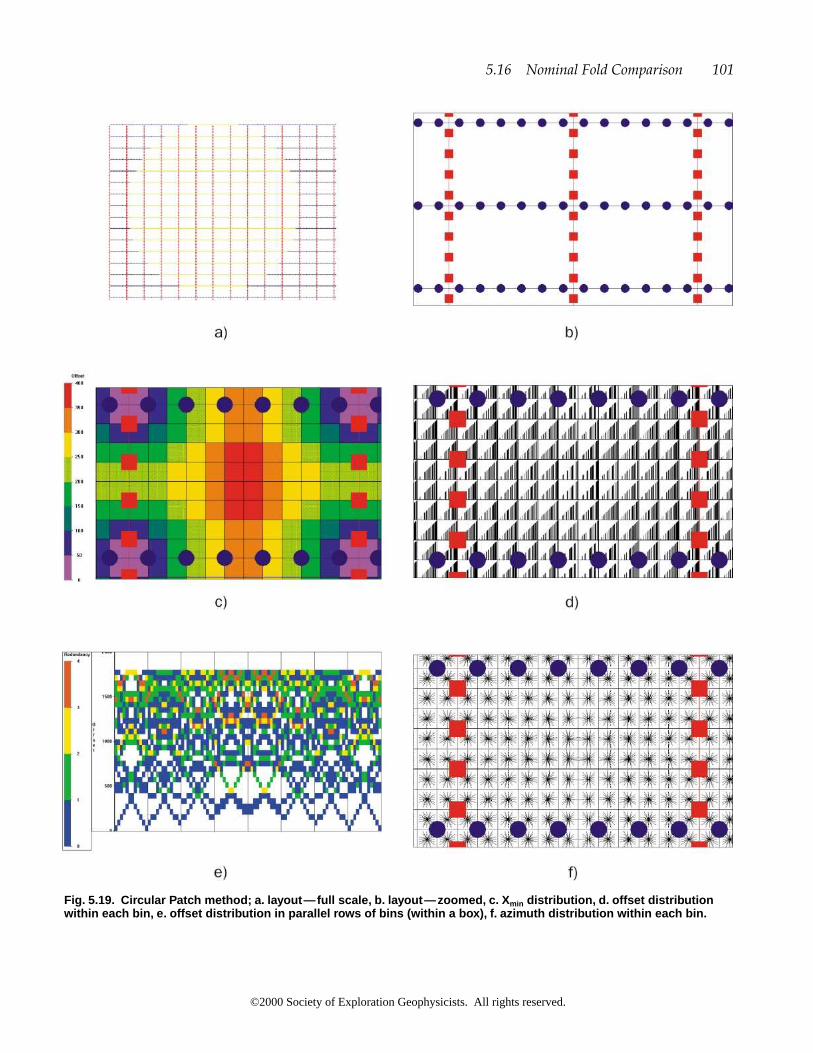
5.16 Nominal Fold Comparison 101
Fig. 5.19. Circular Patch method; a. layout—full scale, b. layout—zoomed, c. Xmin distribution, d. offset distributionwithin each bin, e. offset distribution in parallel rows of bins (within a box), f. azimuth distribution within each bin.
©2000 Society of Exploration Geophysicists. All rights reserved.

102 Field Layouts
Fig. 5.20. Full-fold comparison; a. Swath, b. Orthogonal, c. Brick, d. Nonorthogonal—45°, e. Nonorthogonal—26.565°,f. Flexi-Bin.
©2000 Society of Exploration Geophysicists. All rights reserved.

5.16 Nominal Fold Comparison 103
Fig. 5.20. (continued) Full-fold comparison; g. Button Patch, h. Zig-zag, i. Megabin, j. Star, k. Radial, l. Random.
©2000 Society of Exploration Geophysicists. All rights reserved.

for these designs have been discussed earlier in thischapter.
The mega-bin design has two lines of fold coveragefor every source line, similar to the swath method(Figure 5.20i). The major differences are that therecording patch now is far greater than with the ear-lier swath method and the line interval is four timesthe bin size. However, one can certainly see the simi-larity between these two designs.
The star and radial designs reach far greater foldin the center of the survey than the nominal 30fold of the other designs (Figures 5.20j, 5.20k). Ittherefore may be desirable to offset the lines some-what in the center or eliminate some source pointsnear the center. The radial design offers far better
fold coverage than the star design toward the edges ofthe survey.
A circular patch produces an even fold distributionsimilar to the earlier Figures 5.20b–5.20h, because itdepends merely on the selection of the offset distanceof receivers to be included (which should be equal toXmute). Any random design creates some higher foldbins at the expense of some lower fold coverage inother bins (Figure 5.20e).
Table 5.1 compares some of the major advantagesand disadvantages of each of the design methods pre-sented in this chapter. It is by no means a complete-treatment; the reader is referred to the individual sec-tions of this chapter for further information.
104 Field Layouts
Table 5.1. Field layouts—pros and cons of various layout strategies.
Layout Pros Cons
Swath Simple geometry. Cost efficient. Poor azimuth distribution.Good offset distribution. Poor statics coupling.Minimum equipment movement.
Orthogonal Simple geometry. Large Xmin .
Brick Smaller Xmin may allow a wider RLI. Access can be a problem.Reasonable offsets and azimuths. Poor sampling in common-receiver gather
can lead to acquisition footprint.
Nonorthogonal Simple geometry. Same as orthogonal.
Flexi-Bin®* or High resolution with low fold, or low Same as orthogonal.Bin Fractionation* resolution with high fold.
Super bins for normal use have good offset and azimuth mix.Excellent statics coupling.
Button Patch* Efficient utilization of large channel systems. Can require large number of source pointsover a wide area for each patch.
Good offset and azimuth distribution require Needs large channel capacity.detailed planning. Static coupling hard to accomplish.
Prone to acquisition footprint.
Zig-Zag Same as brick. Efficient for equipment moves. Must have very open access.Single zig-zags are prone to acquisition foot-print
Mega-Bin* Improved noise sampling. Similar to swath method.Must f-x interpolate to fill empty bins.
Star and Radial Good for salt domes. Best with all lines live.Offers excellent offsets for migration. Highly irregular statistics.
Random Improved offset and azimuth distribution. Fold, Xmin and Xmax are more random.Minimal acquisition footprint.
Circular Patch Consistent Xmax . Operationally difficult.
*Patent Restrictions apply to the use of these technologies.
©2000 Society of Exploration Geophysicists. All rights reserved.

Chapter 5 Quiz
1. Where is the bin that contains the largest mini-mum offset in an orthogonal design?
2. What does the largest minimum offset in a brickpattern design depend on?
3. What is the basic concept of Flexi-Bin®?
4. What is essential for the application of the zig-zag method?
5. What is the difference between a star and a ra-dial layout?
5.16 Nominal Fold Comparison 105
©2000 Society of Exploration Geophysicists. All rights reserved.

©2000 Society of Exploration Geophysicists. All rights reserved.
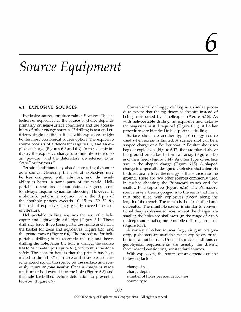
6.1 EXPLOSIVE SOURCES
Explosive sources produce robust P-waves. The se-lection of explosives as the source of choice dependsprimarily on near-surface conditions and the accessi-bility of other energy sources. If drilling is fast and ef-ficient, single shotholes filled with explosives mightbe the most economical source option. The explosivesource consists of a detonator (Figure 6.1) and an ex-plosive charge (Figures 6.2 and 6.3). In the seismic in-dustry the explosive charge is commonly referred toas “powder” and the detonators are referred to as“caps” or “primers.”
Terrain conditions may also dictate using dynamiteas a source. Generally the cost of explosives may be less compared with vibrators, and the avail-ability is better in some parts of the world. Heli-portable operations in mountainous regions seem to always require dynamite shooting. However, if a shothole pattern is required, or if the depth of the shothole pattern exceeds 10–15 m (30–50 ft), the cost of explosives may greatly exceed the cost of vibrators.
Heli-portable drilling requires the use of a heli-copter and lightweight drill rigs (Figure 6.4). Thesedrill rigs have three basic parts: the frame and mast,the basket for tools and explosives (Figure 6.5), andthe prime mover (Figure 6.6). The procedure for heli-portable drilling is to assemble the rig and begindrilling the hole. After the hole is drilled, the sourcehas to be “made up” (Figure 6.7), which must be donesafely. The concern here is that the primer has beenmated to the “shot” or source and stray electric cur-rents could set off the source on the surface and seri-ously injure anyone nearby. Once a charge is madeup, it must be lowered into the hole (Figure 6.8) andthe hole back-filled before detonation to prevent ablowout (Figure 6.9).
Conventional or buggy drilling is a similar proce-dure except that the rig drives to the site instead ofbeing transported by a helicopter (Figure 6.10). Aswith heli-portable drilling, an explosive and detona-tor magazine is still required (Figure 6.11). All otherprocedures are identical to heli-portable drilling.
Surface shots are another type of energy sourceused when access is limited. A surface shot can be ashaped charge or a Poulter shot. A Poulter shot usesbags of explosives (Figure 6.12) that are placed abovethe ground on stakes to form an array (Figure 6.13)and then fired (Figure 6.14). Another type of surfaceshot is the shaped charge (Figure 6.15). A shapedcharge is a specially designed explosive that attemptsto directionally force the energy of the source into theground. There are two other sources commonly usedin surface shooting: the Primacord trench and theshallow-hole explosive (Figure 6.16). The Primacordsource uses a trench gouged into the earth that has athin tube filled with explosives placed along thelength of the trench. The trench is then back-filled anddetonated. The minihole source is similar to conven-tional deep explosive sources, except the charges aresmaller, the holes are shallower (in the range of 2 to 5m deep), and smaller, more mobile drill rigs are used(Figure 6.17).
A variety of other sources (e.g., air gun, weight-drop, p-shooter) are available when explosives or vi-brators cannot be used. Unusual surface conditions orgeophysical requirements are usually the drivingforce toward considering nonstandard sources.
With explosives, the source effort depends on thefollowing factors:
charge sizecharge depthnumber of holes per source locationsource type
107
6Source Equipment
©2000 Society of Exploration Geophysicists. All rights reserved.

108
Fig. 6.1. Detonator.
Fig. 6.2. Explosive charge.
Fig. 6.3. Explosive charges in storage boxes.
Fig. 6.4. Helicopter transport of drilling rig.
Fig. 6.5. Tool basket.
©2000 Society of Exploration Geophysicists. All rights reserved.
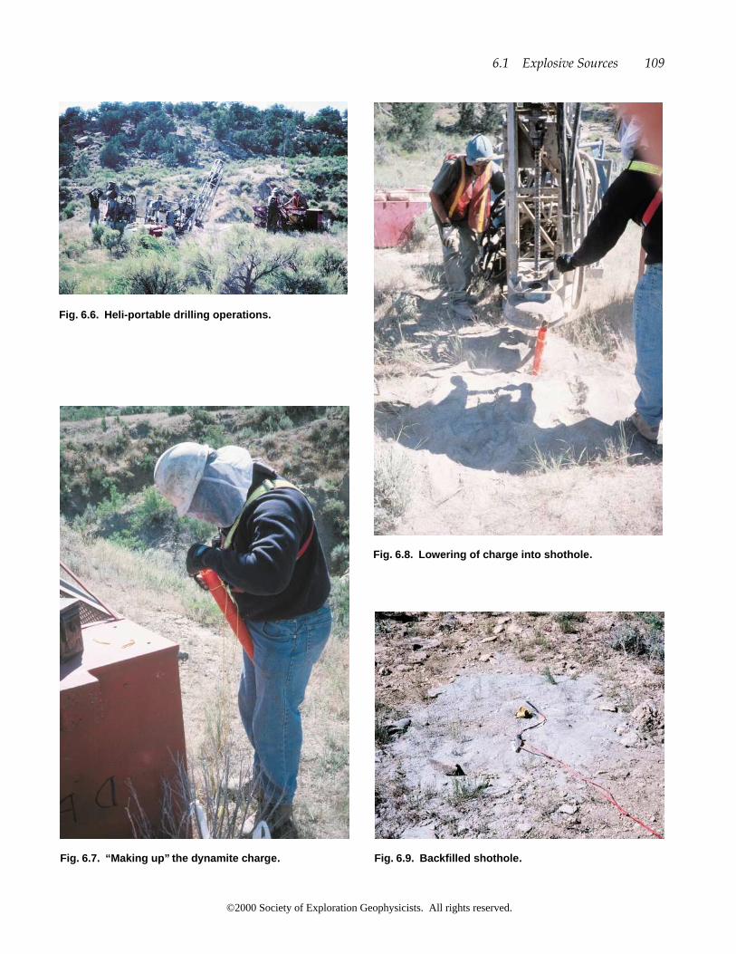
6.1 Explosive Sources 109
Fig. 6.6. Heli-portab le drilling operations.
Fig. 6.7. “Making up” the dynamite charge.
Fig. 6.8. Lowering of charge into shothole.
Fig. 6.9. Backfilled shothole.
©2000 Society of Exploration Geophysicists. All rights reserved.

110 Source Equipment
Fig. 6.10. Con ventional drilling rig.
Fig. 6.11. Explosive and detonator magazine.
Fig. 6.12. Poulter bag.
Fig. 6.13. Poulter source array.
©2000 Society of Exploration Geophysicists. All rights reserved.

The choice of charge size depends largely on thedepth to the horizon of interest. The best charge sizeis that which achieves the maximum signal-to-noiseratio (S/N) at the target depth. Deeper targets usuallyrequire larger charge sizes. However, one should notchoose a charge size that causes shotholes to blow-out, because ejecting mud and wire out of the shot-hole loses a high percentage of the energy. A blowoutcan be dangerous because the drill hole acts like thebarrel of a gun and concentrates the energy released.In addition, the detonator wire is usually ejected fromthe hole, and this wire can short out overhead powerand telephone lines. Generally, larger charge sizescause more ground roll and air blast contamination ofthe record (Figure 6.18). Alternatively, smaller chargesizes mean higher frequency content, but less energygoing into the ground. Recently companies are usinglarger charge sizes again to put more energy into theground. The overall frequency response can be higherthan for smaller charge sizes, although the monitorrecords may appear to have a lower dominant fre-quency content (Figure 6.19). Deconvolution enhances
6.1 Explosive Sources 111
Fig. 6.14. Poulter shot.
Fig. 6.16. Different source types.
Fig. 6.17. Small drilling rig for minihole explosives.
Fig. 6.15. Shaped charge source array.
©2000 Society of Exploration Geophysicists. All rights reserved.

the frequency content such that the bandwidth will behigher and have an improved S/N compared to arecord with a smaller charge size.
The charge depth depends on the depth of theweathering layer and the level of noise interferenceone encounters when testing. Generally, the shallowerthe source (e.g., 6 m or 20 ft), the stronger the air-blastand the ground roll. On the other hand, it is usuallynot economical to go much beyond 50 m (160 ft)depth. If the drilling is really tough and expensive(e.g., basalts or carbonates at surface), one may have
to limit the shothole depth to as little as 2 m (6 ft), or asurface shot may be used instead.
The number of holes per source location dependson the hole depth that one can drill economically andthe apparent noise on single-hole records. Multi-ple-hole patterns may be required for sufficient energy penetration into the ground if difficult drilling dictates that shallow shotholes be used, or fornoise cancellation purposes. In 3-D operations asource array will often be oriented in the same direction as the source lines for best noise cancella-tion, because receiver arrays are generally laid out in-line with the receiver line direction (See Chapter 8—Arrays).
The source type controls the sharpness and dura-tion of the seismic impulse. Explosives are measuredin terms of velocity of propagation, or the speed atwhich the shock wave propagates through the explo-visve material. On one extreme, there is Pentolite, avery quick explosive with a detonation velocity of8300 m/s (27 000 ft/s) that tends to produce a verysharp, short-duration impulse rich in high frequen-cies. In the middle of the velocity spectrum are seis-gel and emulsion-based sources such as 60% Seis-gel.These sources have a velocity of about 5200 m/s (17 000 ft/s), and tend to give a slightly broaderwavelet than Pentolite. The main advantage of thegels over the Pentolite is the quick degradation of thecharge to inert matter in case of a misfired shot. Onthe slow end of the spectrum is Primacord, which candetonate as slowly as 1500 m/s (5000 ft/s) and creates
112 Source Equipment
Fig. 6.18. Monitors showing (a) low-frequency groundroll and (b) high-frequency air blast.
Fig. 6.19. Comparison of small and large charge.
Table 6.1. Typical dynamite test sequence.
Test No. Charge Size Depth No. ofHoles
kg lb m ft
Test for chargesize:
1 0.5 1 15 45 12 1 2 15 45 13 2 5 15 45 14 4 10 15 45 1
Test for depth:5 1 2 6 20 16 1 2 9 30 1
Test for numberof holes:
7 1 2 15 50 38 1 2 15 50 5
©2000 Society of Exploration Geophysicists. All rights reserved.

a long duration explosion. These different explosivesform a variety of possible sources that can be used inthe field and only careful testing can tell which one isbest for each survey.
6.2 DYNAMITE TESTING
Unless acquisition parameters are well known, atest sequence similar to the one in Table 6.1 is recom-mended. The test program should be located 30 to 40stations from a BOL or EOL (beginning/end of line).Charge sizes are in kg (lb). The test results should bedelivered to the processor as soon as possible afterrecording so that the results can be reviewed in detail.The testing will aid in determining what source para-meters should be used for the present program or anyfuture surveys. These test parameters may varygreatly from area to area, and therefore, one shouldassure that the test sequence is suitable for the areaunder investigation.
6.4 Vibrators 113
6.3 DYNAMITE SHOOTING STRATEGY
A major advantage of dynamite operations is thatseveral shooting crews can operate in tandem, shoot-ing alternately (Figure 6.20). This technique allowsone shooting crew to move to the next source locationwhile the other shooting crew is making the electronicconnection between the blaster and the dynamite wireand taking the shot. In dynamite operations it is espe-cially important that vehicles “steady-up” while therecorder is in the listen mode following the shot. Carsor trucks traveling close to the line spread need tostop and shut off their engines to reduce the noise onthe recorded data.
6.4 VIBRATORS
Vertical vibrators (Figure 6.21) produce an asym-metric radiation pattern of P-waves and S-waves.Horizontal vibrators produce weak P-waves and ro-
Fig. 6.20. Tandem shooting on two parallel source lines. Fig. 6.21. Vibrator base plate.
©2000 Society of Exploration Geophysicists. All rights reserved.

bust S-waves. If multiple dynamite patterns do notput enough energy into the ground, vibrators may bepreferred on technical grounds, regardless of relativecost. For example, one may encounter poor dynamitedata in an area with 200 m (650 ft) of glacial till, butstill obtain outstanding data when a Vibroseis sourceis used.
Vibrators are designed in two basic groups: buggy-mounted and truck-mounted units. The buggy vibra-tor (Figure 6.22) is usually more mobile and causesless damage off-road than a truck-mounted vibrator.Most buggy vibrators are pivoted, or swivel behindthe cab, and many can also pivot vertically behind thecab. This maneuverability and flexibility allows forless environmental impact and improved ease of use.On the downside, buggy vibrators must be trucked(Figure 6.23) and can get stuck in fine sand. The truck-mounted vibrator (Figure 6.24) is more efficient forroadwork and use around more developed areas. Thetruck-mounted vibrator does not perform as well off-road as a buggy, so vibrator choice is usually dictatedby the project logistics.
6.5 VIBRATOR ARRAY CONCEPTS
In vibrator acquisition, the source effort depends onthe following parameters:
sweep lengthnumber of sweepsnumber of vibratorsfundamental ground force
The sweep length (time) is usually in the range of 4to 20 s. Testing will determine the combination ofsweep length with the other acquisition parametersthat offer the best results. The longer the sweeplength, the more time the vibrators spend putting cer-tain frequency ranges into the ground. A long sweepcan be good from an energy/bandwidth point ofview and also bad because long sweeps can some-times create significant ground roll and other noise.
The number of sweeps summed at each source sta-tion may range between 4 and 20. Noise cancellationis improved by increasing the number of sweeps. Forexample, wind noise on far traces can be reduced sig-nificantly with a higher number of sweeps.
The product of the sweep length and the number ofsweeps is referred to as the pad time and is one of themost important factors in determining the crew cost:
(6.1)
Pad time usually varies between 64 and 144 s persource point; however, under certain circumstances, itmay be as low as 10 s. Generally, it is more economi-cal to decrease the number of sweeps because that re-duces the vibrator moves. Fewer and longer sweeps
pad time � (sweep length) � (number of sweeps)
114 Source Equipment
Fig. 6.22. Vibrator—bug gy mounted.
Fig. 6.23. Vibrator transport.
Fig. 6.24. Vibrator—truck mounted.
©2000 Society of Exploration Geophysicists. All rights reserved.

are more desirable than are increased numbers ofshort sweeps.
The number of vibrators usually varies between 3and 5 per array (Figure 6.25), and most crews are run-ning two vibrator arrays per acquisition crew. Acquir-ing data with single or dual vibrators will not offerthe noise cancellation that can be accomplished with alarger number of vibrators. Because vibrator data al-most always use source arrays, one should alwaysconsider using receiver arrays (see Chapter 8) on vi-brator surveys.
The fundamental ground force is the last factor af-fecting vibrator effort. Along with the number of vi-brators, the ground force produced by a vibrator af-fects the S/N far more than sweep length, number ofsweeps, and bandwidth according to the followingformula (Malcolm Lansley, pers. comm.):
S/N improvement in dB � 20 log (number of vibra-tors � fundamental ground force � (sweep length� number of sweeps � bandwidth of sweep)1/2).
(6.2)
Vibrators can be spread over a great distance to cre-ate a source pattern, and many sweeps can besummed to create a large source. A continuous succes-sion of pad locations results (Figure 6.26). The dis-tance from the pad of the first vibrator to the pad ofthe last vibrator determines the array length. This ar-ray may be stationary or can be moved up over a pre-determined distance about the source point as shownin Figure 6.27. The total source array length is
effective source array length � array length � totalmove-up � number of vibrators � pad distance �
number of move-ups � move-up distance. (6.3)
Example: effective source array length �
4 � 10 m � 3 � 10 m � 70 m
or
effective source array length �
4 � 41 ft � 3 � 41 ft � 288 ft.
6.5 Vibrator Array Concepts 115
Fig. 6.25. Vibrator array.
Fig. 6.26. Vibrator pad marks. Fig. 6.27. Vibrator array, move-up, and drag.
©2000 Society of Exploration Geophysicists. All rights reserved.

Move-up attenuates noise and is easier on opera-tors, equipment, and the environment. A smallamount of move-up may decrease air blast noise andground roll at near offsets. Larger move-ups may in-crease multiples and should be avoided.
Often the first vibrator sits near the source flag forthe first sweep. The vibrator array then moves up be-tween each sweep so that the last vibrator sits nearthe flag for the final sweep. This vibrator movementcreates a weighted array (in Figure 6.27 the weightsare 1, 2, 3, 4, 3, 2, 1). If, after the final sweep, the firstvibrator is not at the next flag, the entire array drivesup to the next flag.
The changes in vibrator coupling that occur whileusing a move-up can be neglected, because the vibra-tor coupling changes from sweep to sweep and evenwithin a sweep from beginning to end.
6.6 VIBRATOR TESTING
Similarity tests (“sims”) are performed at leasttwice daily to confirm that vibrators are performingsatisfactorily. Hard-wire tests, with a physical cableconnection from the recorder to the vibrators, are themost thorough performance check and these should
116 Source Equipment
Table 6.2. Typical vibrator test sequence.
Test No. of Sweep Number Sweep Dwell Array Move Totalno. vibrators frequency of length dB/octave length -up array
(Hz) sweeps (s) (m) (m) (m)
Test for sweep frequency1 4 10–80 8 12 3 30 30 60
3 4 10–100 8 12 3 30 30 604 4 10–110 8 12 3 30 30 605 4 10–120 8 12 3 30 30 60
Test for dwell6 4 10–90 8 12 none 30 30 607 4 10–90 8 12 6 30 30 60
Test for drag length8 4 10–90 8 12 3 30 10 409 4 10–90 8 12 3 30 20 50
10 4 10–90 8 12 3 30 30 60
Test for number of sweeps11 4 10–90 1 12 3 30 30 6012 4 10–90 2 12 3 30 30 6013 4 10–90 4 12 3 30 30 6014 4 10–90 16 12 3 30 30 6015 4 10–90 32 12 3 30 30 60
Test for sweep length16 4 10–90 8 4 3 30 30 6017 4 10–90 8 8 3 30 30 6018 4 10–90 8 16 3 30 30 6019 4 10–90 8 32 3 30 30 60
Test for number of vibrators20 1 10–90 8 12 3 0 0 021 2 10–90 8 12 3 10 0 1022 3 10–90 8 12 3 20 0 2023 4 10–90 8 12 3 30 0 30
603030312810–9042
©2000 Society of Exploration Geophysicists. All rights reserved.

be completed at the start of the job and anytimeequipment is pulled offline for maintenance or repair.Vibrator testing usually requires a significant amountof time in the field to record different kinds of sourceparameters; e.g., varying the sweep range, dwell, draglength, number of sweeps, sweep length, boost orgain percentages, peak force, and number of vibra-tors. Unless acquisition parameters are well known, atest sequence similar to the one in Table 6.2 is recom-mended. A standard sweep might be that indicated astest no. 2. The type of test sequence may vary greatlyfrom area to area. The S/N formula can be used to de-sign a test sequence so that the parameters vary suffi-ciently to show S/N variations that are easily visible.In Table 6.2 this requirement has been incorporated byincreasing the number of sweeps and the sweeplength by factors of 2. The improvement in the S/Nshould be 3 dB with each doubling of effort [see equa-tion (6.2)].
It is important for vibrator testing to have a fieldprocessing system that will allow the geophysicist tomake on-the-spot decisions about further testing thatmay be necessary beyond an initial test sequence.Band-pass filters of deconvolved shot records give agood indication of the necessary sweep range. Thequality control geophysicist must ensure that the fieldprocessing system can interface with the recordingsystem. The most basic questions in this age of chang-ing recording media are: Are the tape drives the same;how long does it take to transfer the information; andis that time reasonable? It is recommended that oncebasic parameters are picked, the first few square kilo-meters of the survey are fast-tracked, processed in thefield, and the results analyzed by the interpreters fordata usability and quality (Duncan et al., 1996). Oneshould retain the test results to reduce the amount oftesting necessary during future programs in the area.
Vibrators can perform sweeps in a wide variety ofoptions. Down-sweeps that were in vogue in the1970s have been replaced by up-sweeps. Up-sweepsstart at a low frequency of about 10 Hz and sweep to80, 100, 120 Hz, or more. Sweeps may be linear, whichmeans an equal amount of time is spent sweepingthrough the frequency ranges, or a dwell or “boost”can be incorporated into the system to allow enhance-ment of higher frequencies (Figure 6.28). Such a dwellcreates nonlinear sweeps. Some dwell is useful in in-creasing the high-frequency range of the final stackedseismic section. However, too much dwell can createnoisy record sections due to lack of low-frequencydata needed for interpretability. The normal dwellrange is between 3 and 6 dB/octave. Careful testing
and design of dwell ensures an optimum S/N(Pritchett, 1994). The choice between linear and non-linear sweeps usually does not affect cost as long asthe pad time remains the same. Vari-sweeps can beused to enhance certain frequencies beyond the dwellin a selective manner. In this technique, several sweepranges are selected to span narrow frequency bandsand then summed.
For vibrators, a sweep rate is established as follows,and this parameter has to be set in the recording truckas well as in the vibrators:
(6.4)
One needs to perform phase, force, and frequencyversus time plots for all vibrators before and aftertesting to evaluate their performance. Figure 6.29shows the performance of four vibrators. Three linesare solid to signify the similarity of those perfor-mances. The poorly performing vibrator is noted as adashed line. The phase versus time plot should indi-cate essentially a constant phase after 1 to 2 s. Anymajor deviation (i.e., � 5°) is unacceptable, as is theone vibrator that shows a somewhat linear change inphase over time (dashed line).
sweep rate �highest frequency � lowest frequency
sweep length.
6.6 Vibrator Testing 117
Fig. 6.28. Linear versus nonlinear sweeps.
©2000 Society of Exploration Geophysicists. All rights reserved.

Vibrators should operate at 70 to 90% of peak force.Each vibrator performs more consistently by operat-ing at such a percentage rather than closer to peakforce. Also, operating at a higher force introduceslarger vibrator-to-vibrator differences, which resultsin poorer quality data. On the other hand, the vibratorforce should not drop below 90% of the operatingforce throughout the sweep (e.g., dashed line). Thefrequency versus time plot in Figure 6.29 indicates anonlinear sweep with three vibrators having similarsweeps, while one vibrator is sweeping with a higherdwell.
The vibrator-sourced data can be recorded in twoways. In normal practice, records are correlated withthe vibrator source signal before putting the recordsto tape. Recording uncorrelated records increases taperequirements by a large amount—a factor of five inthis example (sweep length of 12 s � the listen time of3 s, i.e., 15 s).
6.7 VIBRATOR DEPLOYMENT STRATEGY
For large surveys, one may want to employ twosets of four or five vibrators to allow more effectivedata acquisition. This source strategy increases thedaily cost but reduces the amount of recording time.The use of several sets of vibrators depends on sev-eral factors, such as the terrain, required sweep effort,and drive time between source points. The fifth vibra-tor in each set can be an in-the-field spare so produc-tion is not lost if a vibrator needs repair. Such contin-gency planning is essential, particularly in remoteareas.
Vibrator surveys have the major advantages thatsource points may be occupied repeatedly to increasethe fold after having moved the patch, or to repeat asource point. This flexibility is much more difficult toachieve with dynamite programs because of shotholedrilling time, patch moves, and confusion over whichholes are to be shot. During vibrator operations, linecrews can still lay out and pick up cables and phones.This crew movement usually cannot take place whilerecording dynamite data.
When source points need to be occupied repeatedly,it is important to strive for nonduplicating source-to-receiver raypaths. This also applies to the recovery ofmake-up source points. Recovery-source-point posi-tioning is also better when the source points are per-pendicular to the source lines rather than parallel tothe line. This station movement reduces disturbancesin the fold distribution.
Slip-sweep acquisition has been instrumental in re-ducing the time spent on vibrator source points. Thisis performed by squeezing more VPs into a givenamount of recording time by letting subsequentsweeps overlap by a certain extent (Rozemond, 1996).
Some Vibroseis surveys are performed with singlesweeps at source stations a short distance apart (e.g.,every 10 m). The data from each of these “sweeps” iscorrelated separately. During processing, these“shots” are treated individually, which leads to foldsas high as 720. The data resulting from such surveys isgenerally of extremely high quality. To date, most ofthese types of surveys have been conducted in theMiddle East.
Allen et al. (1998) presented a new method of high-fidelity recording using vibrators which includes thesimultaneous recording of data from several vibra-tors. Processing such data uses measured motion sig-nals on vibrators to separate the data for each vibratorand has resulted in higher fold data with a significantimprovement in the data quality (Wilkinson et al.,1998).
118 Source Equipment
Fig. 6.29. Phase, force, and frequency versus time qual-ity-control plots.
©2000 Society of Exploration Geophysicists. All rights reserved.

6.8 OTHER SOURCES
Although dynamite and vibroseis are used on thegreat majority of surveys, other sources can be andare used in the field for 3-D surveys, such as:
air guns and mud guns (used in transition zone surveys)
shotgun (Betsy)Mini-Sosie (thumper)land air-gunDinoseisElastic Wave Generator—EWG (Bison)Mini-Vibes
It is possible to use one of these (environmentallynoninvasive) surface sources in certain parts of the 3-
D survey to collect near-offset (shallow) data where itis impossible to use dynamite or Vibroseis. Heavier(stronger) sources can collect long-offset (deep) databy undershooting those parts. The processing centerwill have the unenviable task of matching the phaseof the shallow and deep data in order to create onedata set.
Chapter 6 Quiz
1. What parameters determine the effort in dyna-mite shooting?
2. What is meant by the expression “pad time”?3. Explain the terms array length and move-up by
drawing a diagram.
6.8 Other Sources 119
©2000 Society of Exploration Geophysicists. All rights reserved.

©2000 Society of Exploration Geophysicists. All rights reserved.

7.1 RECEIVERS
The receiver type depends on the characteristics ofthe data to be recorded and the environment wherethe data acquisition occurs. A variety of receivers andtheir uses are listed in Table 7.1. In normal land opera-tions, geophones have a resonant frequency of 10 or14 Hz, but in some parts of the world it is still normalpractice to use 6- or 8-Hz phones. However, geo-phones with resonant frequencies up to 40 Hz are be-ing manufactured (Figure 7.1). Receivers are usuallywired in groups of 1, 4, 6, 9, 12, or 24 (Figure 7.2).While the trend is towards higher numbers of phones(9, 12, 24—or even 72 in the Middle East), lower num-bers (e.g., 6) are still used in certain areas, e.g., SouthAmerica. If the takeouts on the receiver line cables arespaced farther apart than the group interval, the ca-bles can be coiled. Geophone stations may be addedas single stations (telemetry systems) or in sets of 4 or6 groups (distributed systems), depending on therecording instrumentation employed. Generally eachgeophone group can be addressed individually fromthe recorder.
New 3-component solid-state receivers are underdevelopment. These sensors will have a digital outputwith a flat spectrum. The micromachined accelerome-ters utilize sigma-delta technology and provide highresolution and ultralow distortion. Since three sensorsare aligned orthogonal to each other, the deployment
angle can be measured directly and any tilt of the sen-sor unit is immaterial.
Future sensor developments should include a sig-nificant weight reduction, allowing much higherchannel capacities to be deployed in less time. In-linesampling might be much closer in the future, withsmaller bins being used and higher fold data beingrecorded.
Receiver arrays are formed by spreading receiversover some distance (e.g., 12 geophones over 20 m or40 to 55 ft). For operational reasons, the groups arelaid out in-line with the recording spread, cross-line,or in a pattern such as a circle or a box, around thestation flag (e.g., Figure 7.3). Little work is available inthe public domain about the use of receiver arrays in3-D seismic recording (Regone, 1994). A box array im-proves the two-dimensional effect of the array, andthe linear dimension of the array is reduced. Cluster-ing of some geophones may create a weighted spread,but reduces the effectiveness of long-wavelengthnoise attenuation. A more complete discussion of ar-rays is provided in Chapter 8.
In hilly terrain, where the height difference betweenthe ends of any receiver group exceeds 2 m or 6 ft,geophones may be clustered in a small area. In steepterrain (over 5 m or 15 ft elevation difference) one canspread the phones out parallel to topographic con-tours to minimize interarray statics smear. The geo-phones may need to be temporarily buried to reducewind noise. For a 3-D survey that may need to bereshot at a later date (e.g., fire-flood monitoring), itmay be best to bury or cement phones permanently inthe ground.
Three-component 3-D recording requires threetimes the number of channels of recording capacitysince each component is recorded separately (Figure7.4, center geophone). This increased number of chan-nels may make it difficult to create a patch that creates
121
7Recording Equipment
Table 7.1. Types of receivers.
Type Resonant Frequency Environment
geophone 6, 8, 10–40 Hz landmarsh phones 10–14 Hz transition zonehydrophones 10–14 Hz marine3-component 2–8 Hz shear wave
©2000 Society of Exploration Geophysicists. All rights reserved.
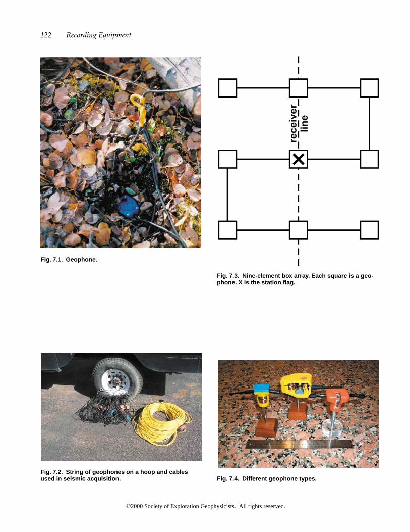
122 Recording Equipment
Fig. 7.1. Geophone.
Fig. 7.2. String of geophones on a hoop and cablesused in seismic acquisition.
Fig. 7.3. Nine-element box array. Each square is a geo-phone. X is the station flag.
Fig. 7.4. Different geophone types.
©2000 Society of Exploration Geophysicists. All rights reserved.

sufficient fold. Since shear-wave reflections contain alower frequency bandwidth, phones with lower reso-nant frequencies are used.
In transition zone environments (shallow marine,marsh, or lake), one may want to use hydrophones ormarsh phones. Marsh phones should be pole plantedto secure the best coupling. Hydrophones can bestrung out in a pattern on the lake bottom. Often theavailable equipment will allow only one receiver ele-ment per group. One has to carefully examine the ef-fect that a one-element array will have on noise reduc-tion. Hydrophones are pressure sensitive rather thanvelocity sensitive as geophones are, and reflectedpressure wavefields are 180° out of phase with re-flected particle-velocity wavefields. The timing rela-tionship between the primary pressure reflection andits ghost causes an apparent 90° phase shift betweenhydrophones relative to geophones at shallow depthsnear the shoreline. Crosscorrelation filters can be de-signed to obtain the best phase match between differ-ent recording instruments and source wavelets.
Once sufficient receiver groups are deployed torecord the first source point, the operator in therecording truck needs to stabilize the spreads by
checking for proper cable connections electronically.Should there be any poor connections or leakages, theline crews need to check, repair, and (if necessary) re-place spread cables, boxes, batteries, and connections.The operator should avoid a total system shutdownonce the spread is stable, because a wake-up acrossthe spread involves rechecking the entire spreadagain, which is rather time consuming (another rea-son for 24-hour operation). However, radio telemetrysystems do not suffer from such problems and fastwake up times are normal because all boxes wake upsimultaneously rather than with a cable system wherea bad box can cause the remainder of the spread pastthe bad box to be inactive.
7.2 RECORDERS
There is a large variety of recording equipmentavailable for 3-D surveys. Today, many acquisitionsystems provide 24-bit recording technology; most ofthe systems listed in Table 7.2 do so. A 24-bit technol-ogy system offers high fidelity because it records dataover a large dynamic range. The listing in Table 7.2
7.2 Recorders 123
Table 7.2. 3-D Recording instrumentation.*
Manufacturer System T/D/R Boxes Stations Line unitsper box
Fairfield Telseis Star T RU 1–6 directly to CRS/CRS CRSFairfield BOX T/D/R RU 1–8 CRSGeo-X Aram D RAM 8 LTU CRUInput/Output I /O I D RSC 6 LTU SCMInput/Output I /O II D MRX 6 ALX SCMInput/Output RSR R RSR 6Input/Output System 2000 D MRX 6 ALX SCMJAPEX G.DAPS-4Sercel Eagle T SAR 1–6 directly to CRS CRSSercel SN388 D SU 1–6 CSU CCUSercel 408 UL T/D/R FDU 1 LAUX CMSyntron Polyseis T RTU
D � Distributed system T � Telemetry system R � Remote seismic recording
ALX Advance line tapCCU Central control unitCLU Cross-line unitCMM Central management moduleCRS Central recording systemCRU Central recording unitCSU Crossing station unitFDU Field data unitLAM Line acquisition moduleLIM Line interface module
LTU Line tap unitMRX Miniature remote signal conditioner, extended
rangeRAM Remote acquisition moduleRSC Remote signal conditionerRTU Radio telemetry unitRU Remote unitSAR Seismic acquisition remote unitSCM System control moduleSU Station unit
*For further specifications please refer directly to the relevant company’s literature.
Centralsystem
©2000 Society of Exploration Geophysicists. All rights reserved.

is not an endorsement of particular instruments butmerely a summary of some technical specifications.Peculiarities for each system need to be examined forthe task at hand, e.g., I/O systems need an additionalLIM when recording more than 1015 channels (1024minus the auxiliary channels). In land operations,these recording units are usually truck or buggymounted and can, therefore, travel easily to areas ofdata acquisition.
Lower channel count systems with higher sam-pling rates, such as the DMT/SUMMIT and the 24-bitOYO DAS, can be used for small, near-surface 3-Dsurveys. In the case of very low channel count sys-tems (e.g., less than 120), it is normal for severalrecorders to be used together in a master-slave sys-tem to reach sufficient channel capacity even forsmall 3-D surveys. There are still a number of 16-bittechnology recorders, but the preference is always touse a 24-bit system. Finally, older analog instrumentslike the DFS V are no longer used for acquiring 3-Dsurveys.
Temporal sampling in 3-D geometry follows thesample theory of 2-D. Usually, one records seismicdata at a 2 ms sample rate with a high-cut of 128 Hzas an anti-alias filter. Resampling to 4 ms is an optionto reduce the data volume before processing, al-though there is a trend towards higher sample rates(e.g., 0.5 or 1 ms). Deeper targets rarely send backhigh frequencies, thus it is illogical to sample deepdata (e.g., more than 2 s two-way time) at a rate lessthan 2 ms.
If a 3-D survey crosses a variety of terrains (e.g.,mountain, plain, transition zone), it is desirable to useone type of recorder to cover all of the survey area.Thus shots of different types (dynamite, airgun, etc.)in the mountains or in the swamp can be recorded bythe same instrument. If more than one recorder isused, amplitude and phase matching will be requiredto compensate for the recorder differences. “Seam-less” receiver coverage from a variety of sources enables application of surface-consistent processes as deconvolution, statics, and amplitude correction. Present industry trends favor such “universal”recording systems.
7.3 DISTRIBUTED SYSTEMS
Distributed systems have cable connections be-tween the units that record the field data and the con-trol system in the recording truck. Usually, these con-nections are made via a line unit (Figure 7.5) thatgathers the information from several different geo-
phone groups. The recording equipment is set up inan arrangement similar to the one in Figure 7.6. Inmost distributed systems, some number of groups ofgeophones are connected to a box. These boxes con-vert the analog signal to digital form (samples). Theboxes are normally wired together along a “branchline” that usually takes the form of a twisted pair.Branch lines feed into cross-line units, which in turnare connected by a “trunk line” and fed directly intothe central recorder (Figure 7.7). In the case of Vibro-seis, the information must be correlated and recordedto tape. This correlation may occur in the individualboxes or at the recording truck (Figure 7.8). Thesetrucks tend to be very cramped with a correlator unit(Figure 7.9), camera units (Figure 7.10), tape drives,and computers that control operations.
124 Recording Equipment
Fig. 7.5. Solar battery powered boxes.
Fig. 7.6. Typical field setup for a distribution system (In-put/Output System Two). ALX � advance line tap, MRX� miniature remote signal conditioner.
©2000 Society of Exploration Geophysicists. All rights reserved.

Fig. 7.7. System control unit.
Fig. 7.8. Recorder.
Fig. 7.9. Correlator unit.
Fig. 7.10. Camera unit and monitor record.
©2000 Society of Exploration Geophysicists. All rights reserved.

7.4 TELEMETRY SYSTEMS
True telemetry systems have no physical connectionbetween the station recording unit and the controlsystem in the recording truck. These systems shouldbe used where access is limited due to rugged terrain,permit problems, or any other reason. A typical fieldsetup is shown in Figure 7.11. Again for convenienceand cross-reference to Table 7.2, the Sercel Eagle sys-tem is illustrated in this example. The SAR (Seismicacquisition remote unit) records the signal and sendsit via radio frequencies to the CRS (Central recordingstation). Telemetry systems have considerable advan-tages over distributed systems, such as:
Reduced HSE (Health, Safety, Environment) im-pact:
No damage to cable from wildlife—or the envi-ronment (e.g., oyster beds)
No cable to carry in rugged (and therefore dan-gerous) terrain
Arbitrary spacing is not a problem
Quicker setup time:
Each box is independent of other boxes; there-fore, shooting can normally be started muchquicker than with a cable system where one badbox can make the rest of the spread inactive.
Better production:
Acquisition does not have to stop because of oneor two bad boxes.
Some telemetry systems (Fairfield BOX and SyntronPolyseis) can receive data in real time. Other telemetrysystems have a disadvantage over distributed systemsin that the radio transmission of the data from the
126 Recording Equipment
Fig. 7.11. Typical field setup for a telemetry system(Sercel Eagle). SAR � seismic acquisition remote unit.
Fig. 7.12. Antenna set-up for telemetry operations.
Fig. 7.13. Remote boxes.
©2000 Society of Exploration Geophysicists. All rights reserved.

boxes to the recording unit takes longer than real time.For some systems, data transmission time may be onthe order of minutes per source point, which may slowdown the shooting crew. Tree cover may also cause aproblem for the signal transmission, and FM interfer-ence may be significant in populated areas. Mixed sys-tems (some telemetry, some distributed) may be usedto cross rivers or roads at select locations.
7.5 REMOTE STORAGE
Some systems have been developed that allow thestorage of many records in the box near the geophonegroups. Examples of these systems are the FairfieldBOX and I/O RSR system. The RSR system is com-posed of a recording truck, a large antenna (Figure7.12), and individual remote seismic recording unitsor “boxes” (Figure 7.13). The data are recorded in thefield and stored in the BOX or RSR box (recordingsfrom several hundred or more source points) and thencollected a few times per week depending on howmuch memory is available. The data collection unit orDCU (Figure 7.14) is temporarily connected to the(BOX or RSR) box and then the stored seismic infor-mation is downloaded to the DCU. After data trans-fer, the memory is erased in the (BOX or RSR) box forfurther use. The DCU is then disconnected from theBOX or RSR and connected to the transcriber and cor-relator unit (Figure 7.15) for further transcription. Thetranscriber then sorts the data to shot records, corre-lates out the pilot sweep, and writes the data to a tapefor permanent storage. In some cases (e.g., FairfieldBOX), the stored data can be collected by radio, oncethe central recorder comes within radio range of theremote storage units. Such a data collection methodcan enormously reduce the HSE impact.
Data QC is difficult or impossible in some cases withremote storage. Ideally, seismic trace attributes shouldbe available for all the traces of a shot shortly after theshot is taken. These attributes (e.g., S/N, rms energy)provide reassurance that good seismic data are beingrecorded. Some remote storage systems can providethis trace attribute information via radio for each shot.
Chapter 7 Quiz
1. What type of receivers should be considered foruse in transition zone environments?
2. What is involved in stabilizing the spread?3. Describe the difference between distributed and
telemetry systems.4. How does a remote seismic recording system
work?
7.5 Remote Storage 127
Fig. 7.14. Data collection unit.
Fig. 7.15. Data transcriber.
©2000 Society of Exploration Geophysicists. All rights reserved.

©2000 Society of Exploration Geophysicists. All rights reserved.

8.1 THE QUESTION OF ARRAYS
Array design in 3-D surveys requires careful con-sideration. A good treatment of arrays in 2-D surveyscan be found in Vermeer (1990). If a receiver array isused, it should be as simple as possible. Circles, boxpatterns, or in-line arrays are commonly used todaybecause of the ease and efficiency of their layout. Adesigner may place a major emphasis on an intricatereceiver array, but this message may be hard to con-vey to the field personnel who may not understandthe necessity of carrying out instructions accurately.In such cases, the designer must work with the fieldpersonnel directly to achieve meticulous placement ofthe arrays.
In 3-D surveys, source energy arrives from manydirections. The array response varies dramatically de-pending on the azimuth between point sources (e.g.,dynamite) and receiver arrays. If geophone arrays arelaid in-line, the response from a point source firedfrom an in-line position will be attenuated, while abroadside source into such an array will not be af-fected by the array. Because of this variation, manycompanies prefer no arrays at all when recording 3-Ddata with single-hole dynamite source points, and useomnidirectional arrays such as circles or clustered ar-rays.
Field tests for linear versus podded geophone ar-rays have indicated that there may be situationswhere arrays can attenuate reflections more thangroundroll does (Wittick, 1998). The tests includedin-line as well as cross-line recording, i.e., the wave-fields hit the geophone groups linearly as well asbroadside.
Regone (1998) has shown that dense wavefieldsampling through the use of areal grids of receivers iseffective in reducing scattered noise. Direct-arrival
noise requires the use of adequate spatial sampling(and usually field arrays), while ambient noise is bestovercome by an appropriate choice of source type,source strength, and fold.
Arrays in the source line direction should comple-ment arrays in the receiver line direction as much aspossible (Vermeer, 1998a). Figure 8.1 shows the differ-ent array combinations that may be considered. Fig-ure 8.1a is a single source point being recorded by alinear receiver array, the series of midpoints indicatespossible smearing in the receiver line direction. Figure8.1b shows the areal midpoint sampling that mighthappen with a combination of linear source and re-ceiver arrays. This areal midpoint coverage issummed as one trace. Figure 8.1c indicates the mid-point coverage that can be achieved with a singlesource and an areal receiver array. The greater thenumber of elements in a receiver array, the larger isthe areal midpoint coverage. Such areal arrays are ef-fective in reducing back-scattered noise.
8.2 GEOPHONE ARRAYS
Figure 8.2 illustrates a five-element geophone arrayresponse oriented east-west to energy arriving fromvarious directions. Figure 8.2a shows the array re-sponse in a linear plot, while Figure 8.2b shows theresponse in a radial presentation. Note the poor atten-uation of broadside energy, at 90° (north) and 270°(south), and good attenuation at 0° (east) and 180°(west). Figure 8.2b shows the 2-D array response with0° being in-line to the geophones, i.e., east-west. Across-sectional display of the array response is shownat the bottom of each figure, e.g. at 209.8° in Figure8.2a. The location of each profile view is indicated bya thick black line through each 2-D response.
129
8Arrays
©2000 Society of Exploration Geophysicists. All rights reserved.

130 Arrays
Fig. 8.1. Midpoint coverage for: a. a single source into a linear geophone array (after Vermeer, 1998a), b. a linearsource array into a linear geophone array, and c. a single source into an areal geophone array.
Fig. 8.2a. Geophone array response (linear).
©2000 Society of Exploration Geophysicists. All rights reserved.

8.3 SOURCE ARRAYS
Figure 8.3 shows an array response of a simulatedfour-vibrator drag in the north-south direction. Notethe good attenuation at 90° (north) and 270° (south)and poor attenuation, or full response, at 0° (east) and180° (west). Typical patterns are four vibrators with 10m between pads (40 m effective array length) movingup 5 m (or less) at a time. In the example of Figure8.3a, the distance between pads is 5 m and move-up is5 m, for a total of four sweeps. The effective arraylength is 35 m; the response of four vibrators is shownas a radial pattern in Figure 8.3b.
8.4 COMBINED ARRAY RESPONSE
Figure 8.4 indicates the combined response of thereceiver and sources arrays. It is important to notethat these graphs are the theoretical response in anideal situation with the geophone arrays and sourcearrays arranged orthogonally. This particular arrayprovides good noise attenuation in all directions. Eachlayout method has its own particular recording geom-
etry. Accordingly, arrays will be laid out differently.The theoretical response should be evaluated beforeproceeding with a particular design.
8.5 STACK ARRAYS
Stack arrays have been discussed by Anstey (1986a,1986b, 1986c, 1987, 1989). The 2-D stack array ap-proach creates an even, continuous, uniform succes-sion of geophones across the CMP gather. In land op-erations, split spreads are used with the followinggeometrical parameters imposed:
group length is equal to the group interval,the source interval is equal to the group interval,
andthe source points are between the groups.
These stack arrays depend on the trace offsets fromtheir respective source points. If isotropic noise is as-sumed, the 3-D stack array becomes a 2-D arrayformed by different offset traces. Thus, the response ateach azimuth is the same. Because 3-D CMP bins al-ways contain traces of differing offsets, the stack array
8.5 Stack Arrays 131
Fig. 8.2b. Geophone array response (radial).
©2000 Society of Exploration Geophysicists. All rights reserved.

132
Fig. 8.3a. Sour ce array response (linear).
Fig. 8.3b. Source array response (radial).
©2000 Society of Exploration Geophysicists. All rights reserved.

133
Fig. 8.4a. Combined 2-dimensional array response (linear).
Fig. 8.4b. Combined 2-dimensional array response (radial).
©2000 Society of Exploration Geophysicists. All rights reserved.

effect is different in each CMP bin and is often negligi-ble because of the irregular offset mix at each CMP.
8.6 HANDS-OFF ACQUISITIONTECHNIQUE
Ongkiehong and Askin (1988) have taken the stackarray approach one step further by imposing equal array lengths for the source and receiver patterns. For symmetric sampling, the number of elements in each array, whether source or receiver, should bethe same. Their conclusion is that any deviation from homogeneity in the fundamental sampling operator is ultimately detrimental. In 3-D field acquisition, such symmetric sampling may not be economi-cally possible, and some compromises need to bemade.
8.7 SYMMETRIC SAMPLING
Vermeer (1998a) supports the idea of symmetricsampling as well. Anything that is done on the re-ceiver side should be done on the source side as well.Hence the source and receiver station as well as lineintervals are equal. The maximum offset is measuredin the in-line direction and it is equal to the maximumoffset measured in the cross-line direction. This re-sults in equal in-line and cross-line fold also. Any re-ceiver arrays are mirrored as source arrays. As men-tioned in the previous section this is an ideal scenario,which requires compromises in practical situations.
134 Arrays
©2000 Society of Exploration Geophysicists. All rights reserved.

9.1 SURVEYING
The designer of the 3-D seismic program and thesurveyors must maintain close communication in or-der to locate the program correctly and execute itproperly. The designer needs to pass on exact instruc-tions for allowances that can be made for any antici-pated changes, e.g., how make-up source points are tobe located. In steep terrain, surveyors often assumethat distance can be measured along the chain (slopechaining), instead of horizontally. Chaining horizon-tally is the only effective way of ensuring that a cen-tral midpoint distribution is maintained (Figure 9.1).
Modern Global Positioning System (GPS) surveyinghas significantly changed the speed of layout and theprecision of acquired survey data in rough terrain.GPS units are usually carried in a backpack (Figure9.2). A hand-held data collector is used to navigate tothe next survey point or the unit can be mounted onan all terrain vehicle (quad) (Figure 9.3) for faster fieldoperations. Many acquisition contractors put regula-tors on the quads to limit the speed of the vehicle forsafety reasons. Along the route to the survey point,the line is flagged and marked for the layout crew tofollow (Figure 9.4).
Vegetation (especially large wet trees) can severelyimpede GPS signal reception. Recently inertial navi-gation systems that can be carried in a backpack havebecome available. These have been used in dense jun-gles with considerable success.
A 3-D seismic design generally goes through threemapping stages: the theoretical plot, the preplot, andthe final plan. The theoretical plot is merely an indica-tion of the theoretical station and line locations (Fig-ure 9.5a). A preplot of the program at a working scalegives the surveyors a good basis to work from andgives the designer the comfort that the anticipated lo-
cation for every source and receiver point has beendocumented (Figure 9.5b). One should number thesource and receiver locations in such a manner that notwo locations have the same number. Topography,wells, buildings, pipelines, existing seismic lines, andother surface culture have an effect on the location ofsource and receiver lines and stations (Table 9.1). Thedesigner takes these into account as much as possiblein the planning stage, especially topographical restric-tions. It is helpful to have the preplot registered withlocal coordinates and possibly overlain on an arealphotograph. The surveyor has to provide detailed in-formation regarding exclusions, skids, and offsets tothe designer, who then decides on the appropriate-ness of the changes and may possibly remodel theprogram. The designer must indicate how far sourcesor receivers may be moved before they should bedropped entirely. Generally, offsetting stations bymore than the line interval is unacceptable. Wherecomplex surface obstacles exist, it might be beneficialto have a designer in the field with the surveyors.Many problems can be solved most easily on the spot.Ideally this advance person has seismic field experi-ence and is equipped with a laptop computer with theinitial 3-D design loaded. The surveyor must establishthe format of the digital survey information prior tothe field visit. The SEG-P1 format is widely acceptedfor this purpose. Standard exchange formats for posi-tional information have been published by the Societyof Exploration Geophysicists (1983). Electronic datatransfer of survey information can significantly re-duce the likelihood of human error when copyingdata.
The final plan uses the actual survey information(Figure 9.5c). The final survey plan of the 3-D pro-gram may not bear much resemblance to the preplot,but it is still an essential element of the surveying
135
9Practical Field Considerations
©2000 Society of Exploration Geophysicists. All rights reserved.

Fig. 9.1. Chaining.
Fig. 9.2. Backpac k GPS unit.
Fig. 9.3. Quad with speed regulator.
Fig. 9.4. Survey flags along seismic line.
©2000 Society of Exploration Geophysicists. All rights reserved.

9.1 Surveying 137
Table 9.1. Sample distance requirements table(Canada/US).
Obstruction Nonexplosive Explosive
Building 50 m 330 ft 180 m 300 ftWater well 100 m 330 ft 180 m 300 ftLow-pressure
pipeline 3 m 3 mHigh-pressure 15 m 300 ft 32 m for � 200 ft
pipeline � 2kg (� 5 lbs)Oil and gas well 15 m 300 ft up to 180 m (depending
on charge size)
output, not only for the processor but also for regula-tory bodies. When final plans for regulatory bodiesare submitted, sometimes they include only approxi-mate line locations and not specific source and re-ceiver coordinates. Final plans should also include in-formation such as access routes and detours that thefield crew can use.
Another technique for handling offset problems iscalled “design on the fly.” When using this technique,the designer works in the field with the permit agents,surveyors, seismic layout crew, and appropriate com-puter resources to adjust for offsets and skips “on thefly.” This technique works best when the designer haspremoved many of the points and compensated withother moves and skids. With all of these premovedpoints loaded into the GPS units and a field designpackage, the designer works in the field with a radioand a computer. When a point needs to be offset, thesurvey crew or the permit crew calls the designer whothen models the offset and compensates by movingother points or offers other possible moves. Theseother moves are tested in the field as the layout pro-gresses. This technique is most effective when there isa good working relationship among all of the differ-ent groups and an excellent radio network is estab-lished.
Map coordinates are usually given using a Univer-sal Transverse Mercator (UTM) projection. The centralmeridian that is used as a reference is an extremelyimportant piece of information. Computer programsfor conversion from one geographic coordinate sys-tem to another are readily available. Knowledge ofthe spheroid, ellipsoid, and details of the projectionare of particular importance for international work.For example, in Argentina a modified UTM grid isused with an origin in the southeast Pacific. In Africa,a different spheroid affects the latitude and longitudeconversion.
Fig. 9.5a. Theoretical layout.
Fig. 9.5b. Preplot example.
Fig. 9.5c. Typical final plan.
©2000 Society of Exploration Geophysicists. All rights reserved.

138 Practical Field Considerations
Table 9.2. Script file example.
This is the beginning of an I /O Script file, converted toASCII, created from FD5.0.
The survey is 3200 m � 3200 m, with 50 m � 50 m binsRLI � 200 m (N/S); SLI � 400 m (E/W); 297 sources 561
receivers; no roll-on; I /O numbering option chosen.HEADER[34bytes]:Script file, software rev: 2.62[2 bytes]10 10Separator:4660 nscripts:297
Serial:101 Stn type:1 Src Type:1Shot Point: LINE: 1.0 STATION: 0.0RECEIVER PATCH: Lowest Line :1 Lowest Stn : 0
Highest Line:16 Highest Stn: 31ACTIVE LINES: 16Line: 1 First Stn: 0 Last Stn: 31Line: 2 First Stn: 0 Last Stn: 31Line: 3 First Stn: 0 Last Stn: 31Line: 4 First Stn: 0 Last Stn: 31Line: 5 First Stn: 0 Last Stn: 31Line: 6 First Stn: 0 Last Stn: 31Line: 7 First Stn: 0 Last Stn: 31Line: 8 First Stn: 0 Last Stn: 31Line: 9 First Stn: 0 Last Stn: 31Line: 10 First Stn: 0 Last Stn: 31Line: 11 First Stn: 0 Last Stn: 31Line: 12 First Stn: 0 Last Stn: 31Line: 13 First Stn: 0 Last Stn: 31Line: 14 First Stn: 0 Last Stn: 31Line: 15 First Stn: 0 Last Stn: 31Line: 16 First Stn: 0 Last Stn: 31
Serial:102 Stn type:1 Src Type:1Shotpoint: LINE: 1.50 STATION: 0.0 - Different source pointRECEIVER PATCH: Lowest Line :1 Lowest Stn : 0
- Same receiver patchHighest Line:16 Highest Stn: 31
ACTIVE LINES: 16Line: 1 First Stn: 0 Last Stn: 31Line: 2 First Stn: 0 Last Stn: 31Line: 3 First Stn: 0 Last Stn: 31Line: 4 First Stn: 0 Last Stn: 31Line: 5 First Stn: 0 Last Stn: 31Line: 6 First Stn: 0 Last Stn: 31Line: 7 First Stn: 0 Last Stn: 31Line: 8 First Stn: 0 Last Stn: 31Line: 9 First Stn: 0 Last Stn: 31Line: 10 First Stn: 0 Last Stn: 31Line: 11 First Stn: 0 Last Stn: 31Line: 12 First Stn: 0 Last Stn: 31Line: 13 First Stn: 0 Last Stn: 31Line: 14 First Stn: 0 Last Stn: 31Line: 15 First Stn: 0 Last Stn: 31Line: 16 First Stn: 0 Last Stn: 31
9.2 SCRIPT FILES
Modern field systems are controlled by script filesthat define how a live patch of receiver stations movesthroughout the entire 3-D program as the source pointsequence progresses. For small 3-D surveys where theentire 3-D is laid out and is live before taking the firstsource point, the sequence of source points is immate-rial. However, on larger 3-D surveys, the progressionof source points is of utmost importance. Time is cru-cial and reoccupying either source or receiver stationshas to be minimized. On larger 3-D surveys, it is com-mon that the number of available channels (geo-phones, cables, and boxes) is at least twice the num-ber of channels in a live patch. This spread capabilityallows for more effective crew operation and patchmovement. If the number of available channels ap-proaches the size of the active patch, the efficiency ofthe crew plummets because the acquisition crewstarts waiting on the layout crew, and standby costsbecome excessive. Managing the available channelsand the efficiency of the layout crew can save signifi-cant amounts of money.
Most computer programs used for designing the 3-D geometry can generate script files. These files canthen be loaded into the field recorder prior to shoot-ing. The operator in the recording truck may havelimited ability to alter script files. One should neverassume that the operator knows how the designer an-ticipates the 3-D survey to be acquired as far as thesource point sequence is concerned. Script files shouldbe tested with the contractor in advance. There areenough idiosyncrasies in the file for mistakes to causeserious delays in the acquisition, and these potentialproblems should be eliminated before the crew isready to start shooting. A meeting between the partychief, observer, and the designer before the crew goesto the field can identify ways to optimize field opera-tions and reduce costs. A typical script file is shown inTable 9.2. Script files are identified by serial numbersor source-point numbers, and then the template is set.The script file does not have to be ordered sequen-tially. Several script file formats are available for ac-quisition systems such as ARAM, Fairfield, I/O, andSercel.
Shell Oil submitted an alternate format for scriptfiles to the SEG for use in the field. This format is referred to as the Shell Processing Support (SPS) format. The SPS files should contain everything that one needs to know about a 3-D survey. The seis-mic processor then knows all the acquisition informa-tion required to process the data. SPS files containfour groups of files:
©2000 Society of Exploration Geophysicists. All rights reserved.

Table 9.3. SPS script file example.
Typical SPS files. Four files are shown on the following pages. This first file is the header file.
H HEADER FILEH00 SPS format version num. SPS001,07.02.95H01 Description of survey area ngal,,N/A,N/AH02 Date of survey 07.02.95,07.02.95H021Post-plot date of issue 07.02.95H022Tape/disk identifier N/AH03 Client N/AH04 Geophysical contractor N/AH05 Positioning contractor N/AH06 Pos. proc. contractor N/AH07 Field computer system(s) GMG/SIS,MESA,Version 1.2H08 Coordinate location N/AH09 Offset from coord. location N/AH10 Clock time w.r.t GMT N/AH12 Geodetic datum,-spheroid N/AH14 Geodetic datum parameters N/AH17 Vertical Datum description N/AH18 Projection type N/AH19 Projection zone N/A,N/AH20 Description of grid units AMERICAN FEETH201Factor to meter 0.30480061H220Long. of central meridian N/AH231Grid origin N/AH232Grid coord. at origin N/AH241Scale factor N/AH242Lat., Long.- scale factor N/AH30 Project code and description N/A,N/A,N/AH31 Line number format N/AH400Type,Model,Polarity 1,N/A,N/A,N/AH401Crew name, Comment 1,N/AH402Sample rate, Record Len. 1,0.000000,N/AH403Number of channels 1,320H404Tape type, format, density 1,N/A,N/A,N/AH405Filter_alias Hz,dB pnt,slope1, N/A,N/A,N/AH406Filter_notch Hz,-3-dB points 1,N/AH407Filter_low Hz, dB pnt slope 1,N/AH408Time delay FTB-SOD app Y/N 1,N/AH409Multi component recording 1,N/AH410Aux. channel 1 contents 1,N/AH411Aux. channel 2 contents 1,N/AH412Aux. channel 3 contents 1,N/AH413Aux. channel 4 contents 1,N/AH600Type,Model,Polarity G1,N/A,N/A,N/AH601Damp coeff,natural freq. G1,N/A,N/AH602Nunits, len(X),width(Y) G1,N/A,N/A,N/AH603Unit spacing X,Y G1,N/A,N/AH700Type,Model,Polarity E1,N/A,N/A,N/AH701Size,vert. stk fold E1,N/AH702Nunits, len(X),width(Y) E1,N/A,N/A,N/AH703Unit spacing X,Y E1,N/A,N/AH711Nom. shot depth,charge len. E1,N/A,N/AH712Nom. soil,drill method E1,N/A,N/AH713Weathering thickness E1,N/AH990R,S,X file quality control 07.02.95,N/A,N/AH991Coord. status final /prov N/A,07.02.95,N/A,N/A
©2000 Society of Exploration Geophysicists. All rights reserved.

S SOURCE POINT FILES1 10011E1 0 0.0 0 0 0.0 1010.7 25.1 0.0 1235959S1 10021E1 0 0.0 0 0 0.0 989.8 44.5 0.0 1235959S1 10031E1 0 0.0 0 0 0.0 971.6 61.3 0.0 1235959S1 10041E1 0 0.0 0 0 0.0 953.0 76.3 0.0 1235959S1 10051E1 0 0.0 0 0 0.0 934.8 95.8 0.0 1235959S1 10061E1 0 0.0 0 0 0.0 919.5 117.9 0.0 1235959S1 10071E1 0 0.0 0 0 0.0 903.6 136.5 0.0 1235959S1 10081E1 0 0.0 0 0 0.0 886.5 149.7 0.0 1235959S1 10091E1 0 0.0 0 0 0.0 860.8 161.1 0.0 1235959S1 10101E1 0 0.0 0 0 0.0 843.1 178.8 0.0 1235959S1 10111E1 0 0.0 0 0 0.0 825.5 196.5 0.0 1235959S1 10121E1 0 0.0 0 0 0.0 807.8 214.2 0.0 1235959S1 10131E1 0 0.0 0 0 0.0 790.1 231.8 0.0 1235959S1 10141E1 0 0.0 0 0 0.0 772.5 249.5 0.0 1235959S1 10151E1 0 0.0 0 0 0.0 754.8 267.2 0.0 1235959S1 10161E1 0 0.0 0 0 0.0 737.1 284.9 0.0 1235959S1 10171E1 0 0.0 0 0 0.0 719.4 302.5 0.0 1235959S1 10181E1 0 0.0 0 0 0.0 701.7 320.2 0.0 1235959
R RECEIVER LOCATION FILER1 10051G1 0 0.0 0 0 0.0 1073.0 72.7 0.0 1235959R1 10061G1 0 0.0 0 0 0.0 1090.7 90.4 0.0 1235959R1 10071G1 0 0.0 0 0 0.0 1108.3 108.1 0.0 1235959R1 10081G1 0 0.0 0 0 0.0 1126.0 125.7 0.0 1235959R1 10091G1 0 0.0 0 0 0.0 1143.7 143.4 0.0 1235959R1 10101G1 0 0.0 0 0 0.0 1161.3 161.1 0.0 1235959R1 10111G1 0 0.0 0 0 0.0 1179.0 178.8 0.0 1235959R1 10121G1 0 0.0 0 0 0.0 1196.7 196.4 0.0 1235959R1 10131G1 0 0.0 0 0 0.0 1214.4 214.1 0.0 1235959R1 10141G1 0 0.0 0 0 0.0 1232.0 231.8 0.0 1235959R1 10151G1 0 0.0 0 0 0.0 1249.8 249.5 0.0 1235959R1 10161G1 0 0.0 0 0 0.0 1267.4 267.2 0.0 1235959R1 10171G1 0 0.0 0 0 0.0 1285.0 284.8 0.0 1235959R1 10181G1 0 0.0 0 0 0.0 1302.8 302.5 0.0 1235959R1 10191G1 0 0.0 0 0 0.0 1320.5 320.2 0.0 1235959
X RELATIONSHIP FILEX0 0111 10241 1 1715 5001 50171X0 0111 10241 18 3416 6001 60171X0 0111 10241 35 5117 7001 70171X0 0111 10241 52 6818 8001 80171X0 0111 10251 1 1716 6001 60171X0 0111 10251 18 3417 7001 70171X0 0111 10251 35 5118 8001 80171X0 0111 10251 52 6819 9001 90171X0 0111 10261 1 1716 6001 60171X0 0111 10261 18 3417 7001 70171X0 0111 10261 35 5118 8001 80171X0 0111 10261 52 6819 9001 90171X0 0111 10271 1 1716 6001 60171X0 0111 10271 18 3417 7001 70171X0 0111 10271 35 5118 8001 80171X0 0111 10271 52 6819 9001 90171X0 0111 10281 1 1716 6001 60171X0 0111 10281 18 3417 7001 70171X0 0111 10281 35 5118 8001 80171X0 0111 10281 52 6819 9001 90171X0 0111 10291 1 1717 7001 70171X0 0111 10291 18 3418 8001 80171X0 0111 10291 35 5119 9001 90171X0 0111 10291 52 68110 10001 100171X0 0111 10301 1 1717 7001 70171X0 0111 10301 18 3418 8001 80171X0 0111 10301 35 5119 9001 90171
Table 9.3. SPS script file example (continued).
©2000 Society of Exploration Geophysicists. All rights reserved.
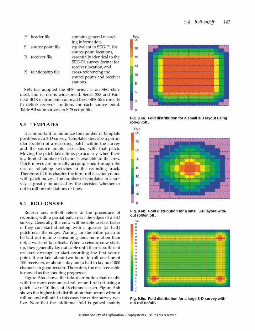
H header file contains general record-ing information,
S source point file equivalent to SEG-P1 forsource point locations,
R receiver file essentially identical to theSEG-P1 survey format forreceiver location, and
X relationship file cross-referencing thesource points and receiverstations.
SEG has adopted the SPS format as an SEG stan-dard, and its use is widespread. Sercel 388 and Fair-field BOX instruments can read these SPS files directlyto define receiver locations for each source point.Table 9.3 summarizes an SPS script file.
9.3 TEMPLATES
It is important to minimize the number of templatepositions in a 3-D survey. Templates describe a partic-ular location of a recording patch within the surveyand the source points associated with that patch.Moving the patch takes time, particularly when thereis a limited number of channels available to the crew.Patch moves are normally accomplished through theuse of roll-along switches in the recording truck.Therefore, in this chapter the term roll is synonymouswith patch moves. The number of templates in a sur-vey is greatly influenced by the decision whether ornot to roll-on/off stations or lines.
9.4 ROLL-ON/OFF
Roll-on and roll-off refers to the procedure ofrecording with a partial patch near the edges of a 3-Dsurvey. Generally, the crew will be able to start fasterif they can start shooting with a quarter (or half )patch near the edges. Waiting for the entire patch tobe laid out is time consuming and, more often thannot, a waste of far offsets. When a seismic crew startsup, they generally lay out cable until there is sufficientreceiver coverage to start recording the first sourcepoint. It can take about two hours to roll one line of100 receivers, or about a day and a half to lay out 1000channels in good terrain. Thereafter, the receiver cableis moved as the shooting progresses.
Figure 9.6a shows the fold distribution that resultswith the more economical roll-on and roll-off using apatch size of 10 lines of 48 channels each. Figure 9.6bshows the higher fold distribution that occurs withoutroll-on and roll-off. In this case, the entire survey waslive. Note that the additional fold is gained mainly
9.4 Roll-on/off 141
Fig. 9.6a. Fold distribution for a small 3-D layout usingroll-on/off .
Fig. 9.6b. Fold distribution for a small 3-D layout with-out roll/on off .
Fig. 9.6c. Fold distribution for a large 3-D survey with-out roll-on/off .
©2000 Society of Exploration Geophysicists. All rights reserved.

through far-offsets, which may not contribute to thefinal stack. If the cross-line dimension is much smallerthan the in-line dimension, one may want to leave oneor two additional receiver lines live when rollingon/off. Figure 9.6c shows the high-fold rim that de-velops in a larger survey when not using roll-on/off(using the same 10 lines of 48 channel patch). Apply-ing an appropriate mute will reduce the fold in thecorners significantly.
Assuming roll-on/off in the in-line direction, thenumber of template positions is calculated as follows(see Figure 9.6a):
(9.1)
Example:
Assuming roll-on/off in the cross-line direction, thenumber of template positions is (see Figures 9.6a and9.7):
(9.2)
Example:
The preceding equation is based on acquiringsource points over only one receiver line interval inthe center of the patch. It is noteworthy that the num-ber of templates is independent of the patch sizewhen rolling on/off lines and stations. The total num-ber of templates is simply the product of the in-lineand cross-line templates:
total number of templates� in-line templates � cross-line templates. (9.3)
Example: 9 � 9 � 81 templates.
Hence with a swath width of one, 81 templateswould be required. The total number of rolls is sim-ply:
total number of rolls � templates � 1. (9.4)
Example: 81 � 1 � 80 rolls.
1800 m
200 m� 9 cross-line templates.
� number of receiver lines � 1.
cross-line templates �cross-line survey size
receiver line interval
2400 m
300 m� 1 � 9 in-line templates.
� number of source lines.
in-line templates �in-line survey size
source line interval� 1
If one can traverse source points over more thanone receiver line interval, the number of cross-linerolls can be reduced. This field procedure is worthconsidering, especially when the number of receiverlines is ten or more (see Section 9.5). If for example, asix-line patch is employed, one can roll over three lineintervals (swath width � 3). The formula for the in-line templates remains as in equation (9.1), while thecross-line template formula changes as follows (as-suming roll-on/off ):
(9.5)
Example:
By increasing the swath width to 3, the number ofrequired templates would be reduced from 81 to 27.
9.5 NO ROLL-ON/OFF
If the patch is equal to or greater than the surveysize, then there is only one template when roll-on/offis not used. In the example of Figure 9.6b, therewould only be one template for a patch of 10 � 48channels. However if the patch is reduced to 8 � 24then the number of templates increases. Assuming noroll-on/off in the in-line direction, the number of tem-plate positions is calculated as follows (see Figures9.6b):
(9.6)
Example:
Assuming no roll-on/off in the cross-line direction,the number of template positions is:
(9.7)
�cross-line survey size � cross-line patch size
receiver line interval� 2
cross-line templates
2400 m � 1200 m
300 m� 1 � 5 in-line templates.
�in-line survey size � in-line patch size
source line interval� 1.
in-line templates
1800 m
200 m � 3� 3 cross-line templates.
�cross-line survey size
receiver line interval � swath width.
cross-line templates
142 Practical Field Considerations
©2000 Society of Exploration Geophysicists. All rights reserved.

Example:
The total number of templates for a 8 � 24 patch isthe product of 5 in-line templates � 3 cross-line tem-plates, i.e., 15 templates in total.
1800 m � 1600 m
200 m� 2 � 3 cross-line templates.
Figure 9.7 shows a further example of a 3-D survey.The number of templates assuming roll-on/off (ornot) for a swath width of one is presented as a prob-lem to be solved for interested readers.
9.6 SWATH WIDTH
The designer has to decide if the template shouldinclude source points over only one receiver line in-terval, or over two, three or more, when the patch isin the middle of the 3-D survey. This technique is called a “Multiline Roll.” The effect on crew speedis different depending on the approach taken. Time isthe main constraint when operating a 3-D crew. It ismost important to minimize the waiting time formovement of recording equipment and source equip-ment (drilling holes or vibrator detours), and to maxi-mize the recording time.
Increasing the swath width decreases the amount ofoverlap with neighboring midpoint areas (see Section5.2). This may have a detrimental effect on the fold,static coupling, offset, and azimuth distributions. Thelarger the swath width, the narrower the azimuth dis-tribution. The far offsets increase also, leading to alarger Xmax although the physical patch size has notchanged. Figure 9.8 indicates how the areas of mid-point coverage change if the swath width is increasedfrom 1 (a) to 3 (b). Xmax can be calculated easily if thecross-line dimension of the patch is taken as twice thecross-line width of the midpoint coverage.
The possible change in the fold distribution is themajor point of consideration. Generally the patch isrolling but for a stationary 12 � 96 channel patch. Fig-ure 9.9 shows the fold distributions with the swathwidth as the only variable (the template is indicated
9.6 Swath Width 143
Fig. 9.7. Patc h moves.
Fig. 9.8. Midpoint coverage for different swath widths (6-line patch): a. swath width 1; b. swath width 3
©2000 Society of Exploration Geophysicists. All rights reserved.

144 Practical Field Considerations
Fig. 9.9. Fold distribution for a 12 � 96 patch with: a. swath width 1, 441 templates, Xmax 3359 m; b. swath width 2, 231templates, Xmax 3503 m; c. swath width 3, 147 templates, Xmax 3653 m; d. swath width 4, 126 templates, Xmax 3807 m; e.swath width 5, 84 templates, Xmax 3965 m; f. swath width 6, 84 templates, Xmax 4127 m.
©2000 Society of Exploration Geophysicists. All rights reserved.
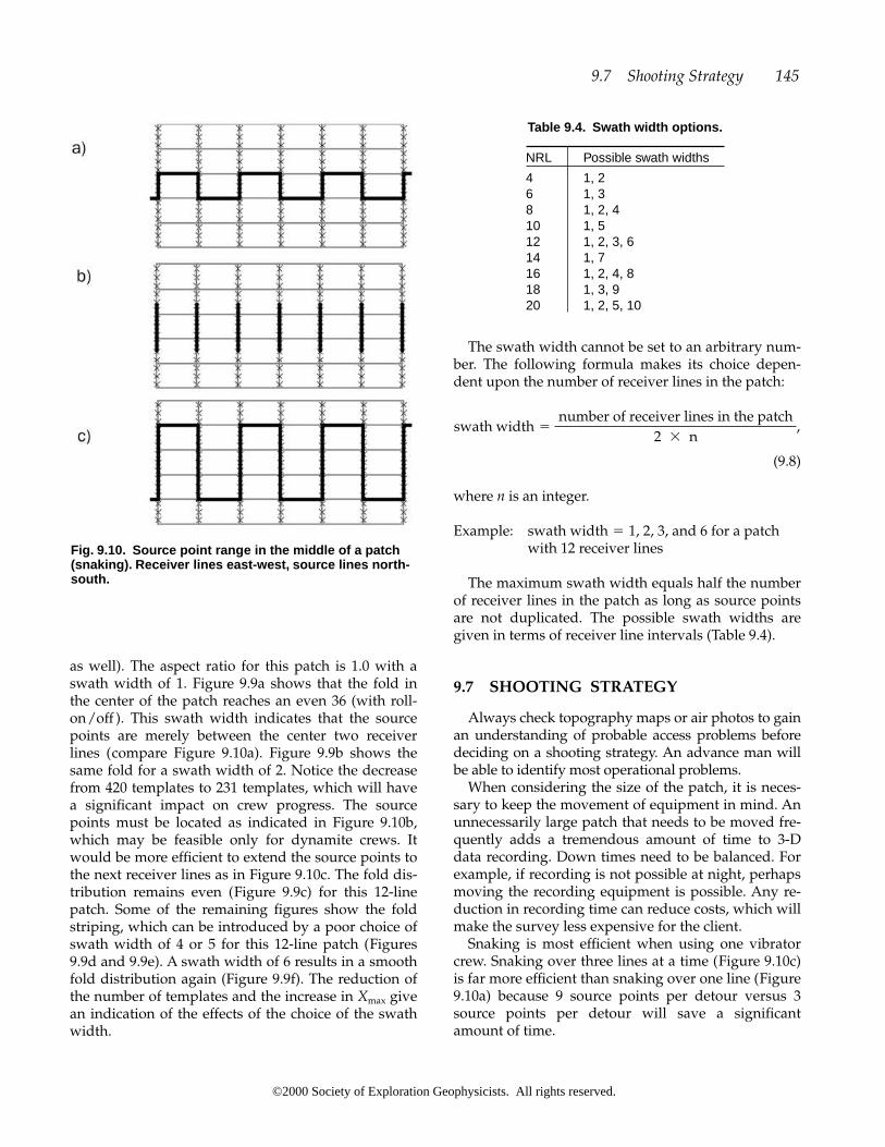
as well). The aspect ratio for this patch is 1.0 with aswath width of 1. Figure 9.9a shows that the fold inthe center of the patch reaches an even 36 (with roll-on/off ). This swath width indicates that the sourcepoints are merely between the center two receiverlines (compare Figure 9.10a). Figure 9.9b shows thesame fold for a swath width of 2. Notice the decreasefrom 420 templates to 231 templates, which will havea significant impact on crew progress. The sourcepoints must be located as indicated in Figure 9.10b,which may be feasible only for dynamite crews. Itwould be more efficient to extend the source points tothe next receiver lines as in Figure 9.10c. The fold dis-tribution remains even (Figure 9.9c) for this 12-linepatch. Some of the remaining figures show the foldstriping, which can be introduced by a poor choice ofswath width of 4 or 5 for this 12-line patch (Figures9.9d and 9.9e). A swath width of 6 results in a smoothfold distribution again (Figure 9.9f). The reduction ofthe number of templates and the increase in Xmax givean indication of the effects of the choice of the swathwidth.
9.7 Shooting Strategy 145
The swath width cannot be set to an arbitrary num-ber. The following formula makes its choice depen-dent upon the number of receiver lines in the patch:
(9.8)
where n is an integer.
Example: swath width � 1, 2, 3, and 6 for a patchwith 12 receiver lines
The maximum swath width equals half the numberof receiver lines in the patch as long as source pointsare not duplicated. The possible swath widths aregiven in terms of receiver line intervals (Table 9.4).
9.7 SHOOTING STRATEGY
Always check topography maps or air photos to gainan understanding of probable access problems beforedeciding on a shooting strategy. An advance man willbe able to identify most operational problems.
When considering the size of the patch, it is neces-sary to keep the movement of equipment in mind. Anunnecessarily large patch that needs to be moved fre-quently adds a tremendous amount of time to 3-Ddata recording. Down times need to be balanced. Forexample, if recording is not possible at night, perhapsmoving the recording equipment is possible. Any re-duction in recording time can reduce costs, which willmake the survey less expensive for the client.
Snaking is most efficient when using one vibratorcrew. Snaking over three lines at a time (Figure 9.10c)is far more efficient than snaking over one line (Figure9.10a) because 9 source points per detour versus 3source points per detour will save a significantamount of time.
swath width �number of receiver lines in the patch
2 � n,
Fig. 9.10. Sour ce point range in the middle of a patch(snaking). Receiver lines east-west, source lines north-south.
Table 9.4. Swath width options.
NRL Possible swath widths
4 1, 26 1, 38 1, 2, 410 1, 512 1, 2, 3, 614 1, 716 1, 2, 4, 818 1, 3, 920 1, 2, 5, 10
©2000 Society of Exploration Geophysicists. All rights reserved.

The direction in which receiver cables are laid outcan dramatically affect the logistics of a survey. If pos-sible, a crew should have enough channels to lay outreceiver lines all the way across one dimension of thesurvey. Entire lines can then be rolled; there is no lossof efficiency in occupying stations twice or more. Inlong skinny surveys, the equipment layout usuallydepends on whether the source is vibrator or dyna-mite. For vibroseis, the shooting is time-consuming,and it is usually better to keep the vibrators movingwhile the geophone (line) crew waits. The reverse istrue for dynamite. Source points can be taken quickly,so one must optimize the equipment (geophones)moves. The line crew should always travel by theshortest possible route. It is important to note that aparticular design might be easy to implement usingvibrators, but not be efficient for dynamite acquisitionand vice versa. Therefore, there may be more than onegood design to meet a particular geophysical objec-tive.
9.7.1 Vibrator
Suppose the long dimension of the 3-D survey isnorth-south (Figure 9.11). For vibroseis source opera-tion, lay out the cable north-south so each line is par-tially laid out and large enough for each patch, andthen shoot across the lines using electronic roll-alongswitches. Once the vibrators have progressed throughhalf the patch, remove short portions of receiver linesfrom the top of the survey and place them at the bot-tom.
9.7.2 Dynamite
For dynamite source operations, the receiver layoutis assumed to be east-west across the short dimensionof the survey (Figure 9.11), and shots are taken until itis time to move an entire line. This procedure is fasterfor the line crew than moving pieces of many lines. Itmakes no difference with regard to fold, offsets, andazimuths if the source and receiver line directions areswitched.
9.8 LARGE SURVEYS
When contemplating large surveys, one has to planhow the seismic crew is allowed to record the data. Alarger survey may require so many receiver stationsalong the receiver line direction that the crew does nothave enough equipment for the number of lines neces-sary for the live patch. One option is to shoot in zippers;
the other is to rent more equipment. In general, unlessthe amount of rental equipment already in use is exces-sive, zippering or redesigning the survey is the less ex-pensive option.
Consider a receiver patch of 8 lines of 100 stationseach. Furthermore, assume that the receiver lines are250 stations long for the entire survey. If the crew hasonly 1000 channels available, one cannot plan a patchof 8 lines of 250 channels each. Essentially, the folddrop of the first segment needs to be overlapped withthe fold build up of the second segment (Figure 9.12).The minimal amount of overlap is shown in the bot-tom part of Figure 9.12. Ideally, the full patch needs tobe available for both segments along the commonsource line, or fold will be reduced and statics cou-pling will be affected adversely. This procedure re-quires reoccupying stations, which is time consumingand costly. One has to decide whether the overlapalong the zipper can be reduced and to what degree.
Often there is a choice of reoccupying source or re-ceiver stations. With vibrators, one may want to re-peat source points without repeating source-to-re-ceiver raypaths. For dynamite acquisition, layingreceivers a second time may be a better alternative, al-
146 Practical Field Considerations
Fig. 9.11. Typical layout for a vibroseis or dynamite sur-vey.
©2000 Society of Exploration Geophysicists. All rights reserved.

though undesirable. The effectiveness and speed ofshooting in zippers depends very much on the swathwidth (see Section 9.5).
The full swath roll constitutes an extremely efficientmethod of template advancement when the 3-D sur-vey is very large and source points are relatively inex-pensive. Source points are occupied twice and all re-ceiver lines are rolled at once in the cross-linedirection. This method allows the contractor to ac-quire very large 3-D surveys with only a limited chan-nel capacity. Note that there are no common receiversfrom one swath to the next. Thus the statics will becompletely indeterminate from one swath to the next.This method of shooting is not recommended if sig-nificant statics are expected.
Doubling the source locations increases the cross-line fold and makes it equal to the number of receiverlines active in the patch instead of half the number ofreceiver lines as in other geometries (see Section 2.5):
cross-line fold � number of receiver lines. (9.9)
Source points for a particular template are both in-side and outside the patch. From the center of thepatch, the source locations extend the following dis-tance away from the central source point:
number of receiver lines � receiver line interval.(9.10)
Therefore, the number of source points that can betaken for one template position of the full swath rollis:
(9.11)
An example of a first template A is shown at the topof Figure 9.13. After taking the source points associ-ated with this template, the receiver patch is ad-vanced in the in-line direction to the end of the surveyas indicated. The entire patch is then rolled a fullswath roll in the cross-line direction as indicated bythe middle template position B in Figure 9.13. In-linerolls are repeated in the opposite direction to the otherend of the survey. The template then advances by an-other full swath roll to the bottom position C in Fig-ure 9.13. The bottom source point of the A template
�2 (NRL) (RLI)
SI.
number of source points per template
9.8 Large Surveys 147
Fig. 9.12. Shooting in zippers (large 3-D surveys).
Fig. 9.13. Full-swath roll.
©2000 Society of Exploration Geophysicists. All rights reserved.

position abuts the top source point of the C templateposition. The source points of the middle template Bare completely overlapped, resulting in the increasedcross-line fold. Although source locations are occu-pied twice, no source-to-receiver raypaths are dupli-cated. In practice, the full swath roll is acquired as de-scribed (often with the source lines extended evenfurther) but is processed as a series of overlappingsymmetric cross-spreads (Vermeer, 1999a). Thus notall shots that were taken into a given receiver spreadare used. The redundancy in data collection (and itsdiscarding by the processor) is more than compen-sated by the high rate of acquisition. In processing,therefore, the minimal data sets are simply overlap-ping cross-spreads (see Chapter 5), and a well-sam-pled 3-D is created (with the exception of the uncou-pled statics described above).
If the minimum offset requirement can be relaxed,it might be possible to not reoccupy source positionsbut rather to interleave the source lines (Figure 9.14).
9.9 FIELD VISITS (QC)
Quality control is necessary in all aspects of thefield operation, including the surveying, chaining,
logging, placement of phones, quality of phoneplants, vibrator synchronization, dynamite loading todepth, accuracy of source and receiver arrays, testingfield parameters, alertness of the crew, and quality ofmonitors. Geophones should be planted vertical tothe Earth’s surface and not vertical to the local slopeof uneven terrain. On a steep slope, arrays should belaid out in-line and parallel to the elevation contoursor be bunched. Generally, elevation difference fromthe first to the last geophone of a group should not ex-ceed 2 m (6 ft).
Bird-dog overseers can represent the client verywell in the area of quality control. They usuallyhave extensive field experience in different roles onseismic crews, having worked through numerouspositions. They know the pitfalls to look for as wellas knowing where a crew may wish to take shortcuts under certain circumstances. The bird-dog vis-its the crew at regular intervals throughout the 3-Dacquisition or is permanently stationed with themfor immediate response to any problems that mayarise.
The designer may also perform a QC role in thefield. Many aspects of the design of a 3-D survey can-not be readily communicated to the acquisition crewor to the bird-dog. Some delays and expensivestandby occurs because of inappropriate decisionsmade in the field. The designer who has a completeunderstanding of the project can quickly and effec-tively make decisions and changes in the field. Keepin mind that at current (2000) prices, an average seis-mic crew costs from $1 to $2 per second in the field.The delay time necessary to drive to town, telephonean offsite designer, explain the problem, develop a so-lution, and implement it in the field may cost tens ofthousands of dollars.
The designer needs to determine how many consec-utive source points may be dropped out of a sourcepoint sequence (e.g., 5 out of 80). Dropped sourcepoints should not be on adjacent source lines. This al-lowance should be made only for reasons of impossi-ble access, pipeline and river crossings, buildings, etc.These missed source points should be substituted, ifat all possible, with make-up shots. Generally theseproblems will be identified ahead of time, but not al-ways. Changing weather conditions can make accessimpossible where previously, in dry weather, access tothe source stations appeared reasonable. The morefreedom the designer and the client can give the con-tractor and the bird-dog, the faster the field crew canoperate. Cooperation among all involved parties isimportant in the efficient acquisition of a 3-D seismicsurvey.
148 Practical Field Considerations
Fig. 9.14. Full-s wath roll, interleaved.
©2000 Society of Exploration Geophysicists. All rights reserved.

9.10 OFFSETS AND SKIDS
When the theoretical source and receiver locationsencounter an obstacle, the stations need to be movedto some other nearby location. It is essential to pro-vide the surveyors with instructions regarding howthe offsets (moves of source or receiver points perpen-dicular to the direction of the line) or the skids (movesof source or receiver points in the direction of the line)are to be performed.
Several priorities can be established (N. Cooper,1997, personal communication). Most important isthat each source point must be taken and each re-ceiver must be located. This requirement maintainsthe average source and receiver point density and theaverage fold. Fold variations are introduced as the off-sets and skids increase; however, these variations areless important than actually dropping the fold levelbecause of missed source points or receiver locations.Priorities might be as follows:
1. Move the source and receiver locations by lessthan of the station interval in each direction—maintaining fold in each bin.
2. Occupy each source and receiver location—maintaining average fold within the survey.
3. Offset up to the line interval—offsetting intro-duces the least amount of fold striping.
4. Skid—skidding introduces more fold stripingthan offsetting (unless skidded by one line inter-val (Donze and Crews, 2000).
5. Do not reoccupy source or receiver locations—duplicate raypaths do not add any valuable in-formation.
1�2
1�2
One can go as far as establishing a specific offsetand skid table for each 3-D design. One example isgiven in Table 9.5. The lower the numbers, the morepreferred this location is as an alternate to the sourcepoint to be moved (see boxed S). This particular tableindicates the preference for offsets rather than skids.This preference decreases as the distance from theoriginal location increases.
When there are several points to offset, it is prefer-able to offset them in a continuous smooth line (e.g.,in an arc of a circle) rather than as large suddenchanges in the amount of offsets and/or skids (Figure9.15). This will produce a smoother change in the shotand receiver gathers in addition to the midpoint dis-tribution in the subsurface and, hence, improve noisecancellation, produce less acquisition footprint, andenhance imaging (Vermeer, 1998a, b).
9.11 GENERAL CONSIDERATIONS
9.11.1 Imaging Area
In deciding how large an area needs to be imaged,several questions should be considered, such as: Whatare the interpreter ’s needs? Are all the wells tied thatneed to be considered? Is the survey big enough tocollect energy from all dipping events? Are the migra-tion apron and fold taper sufficiently large? It may benecessary to place extra source points outside the re-ceiver area to accomplish some of these objectives.There may be some areas of the survey that cost a pre-mium per unit area because of poor access or expen-sive permits. A decision must be made about whether
9.11 General Considerations 149
Table 9.5. Offset and skid chart for a particular 3-D layout.
21 20 S 18 17 16 15 14 13 12 11 10 S 10 1120 19 S 17 16 15 14 13 12 11 10 9 S 9 1019 18 S 16 15 14 13 12 11 10 9 8 S 8 9R R R/S R R R R R R R R R R/S R R
17 16 S 14 13 12 11 10 9 8 7 6 S 6 713 12 S 10 9 8 7 6 5 4 3 2 S 2 317 16 S 14 13 12 11 10 9 8 7 6 S 6 718 17 S 15 14 13 12 11 10 9 8 7 S 7 819 18 S 16 15 14 13 12 11 10 9 8 S 8 920 19 S 17 16 15 14 13 12 11 10 9 S 9 1021 20 S 18 17 16 15 14 13 12 11 10 S 10 11R R R/S R R R R R R R R R R/S R R
19 18 S 16 15 14 13 12 11 10 9 8 S 8 915 14 S 12 11 10 9 8 7 6 5 4 S 4 519 18 S 16 15 14 13 12 11 10 9 8 S 8 9
R � receiver location; S � source point.
©2000 Society of Exploration Geophysicists. All rights reserved.
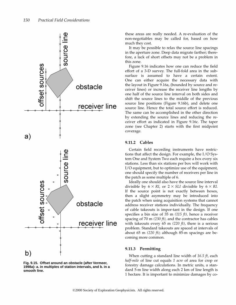
these areas are really needed. A re-evaluation of thenon-negotiables may be called for, based on howmuch they cost.
It may be possible to relax the source line spacingsin the aperture zone. Deep data migrate farther; there-fore, a lack of short offsets may not be a problem inthis zone.
Figure 9.16 indicates how one can reduce the fieldeffort of a 3-D survey. The full-fold area in the sub-surface is assumed to have a certain extent. One can either acquire the necessary data with the layout in Figure 9.16a, (bounded by source and re-ceiver lines) or increase the receiver line lengths byone half of the source line interval on both sides andshift the source lines to the middle of the previoussource line positions (Figure 9.16b), and delete onesource line. Hence the total source effort is reduced.The same can be accomplished in the other directionby extending the source lines and reducing the re-ceiver effort as indicated in Figure 9.16c. The taperzone (see Chapter 2) starts with the first midpointcoverage.
9.11.2 Cables
Certain field recording instruments have restric-tions that affect the design. For example, the I/O Sys-tem One and System Two each require a box every sixstations. Less than six stations per box will work withI/O equipment, but to optimize use of the equipment,one should specify the number of receivers per line inthe patch as some multiple of 6.
Ideally one should also have the source line intervaldivisible by 6 � RI, or 2 � SLI divisible by 6 � RI. If the source point is not exactly between boxes, then a slight asymmetry may be introduced into the patch when using acquisition systems that cannotaddress receiver stations individually. The frequencyof cable takeouts is impor-tant in the design. If onespecifies a bin size of 35 m (115 ft), hence a receiverspacing of 70 m (230 ft), and the contractor has cableswith takeouts every 65 m (220 ft), there is a seriousproblem. Standard takeouts are spaced at intervals ofabout 65 m (220 ft); although 85-m spacings are be-coming more common.
9.11.3 Permitting
When cutting a standard line width of 16.5 ft, eachhalf-mile of line cut equals 1 acre of area for crop orforestry damage calculations. In metric units, a stan-dard 5-m line width along each 2 km of line length is1 hectare. It is important to minimize damages by co-
150 Practical Field Considerations
Fig. 9.15. Offset around an obstacle (after Vermeer,1998a): a. in multiples of station intervals, and b. in asmooth line.
©2000 Society of Exploration Geophysicists. All rights reserved.

operating with landowners. Fence cuts and accessroutes should be used only when absolutely neces-sary, and one must always have prior written permis-sion to access private lands.
Low impact seismic (LIS) guidelines were intro-duced in Canada in 1993. Source line widths must bekept to 5 m (6 m for vibrators) and receiver linewidths to 1.5 m if hand-cut or to 3 m if cat-cut (if al-lowed). Generally, only trees that block the line ofsight are removed. Geophones are usually carried inby hand, flown in by helicopter, or brought in onquads (ATVs). For narrow source lines, dynamiteholes may need to be hand-drilled. The minimal soildisturbance of LIS programs benefits the regrowth oftree cover and impacts wildlife habitat less than stan-dard line cutting. However, line cutting under LISguidelines may cost as much as 30% more than stan-dard line cutting (Wiskel, 1995).
9.11.4 Safety
The safety of the crew must be considered in the de-sign of the survey. Subtle moves of the receiver andsource points have insignificant effects on the foldand offset distribution but can make jobs much safer.For example, if the computer design puts the theoreti-cal location on a rocky slope or a cliff, it might be bestto move the point to a flatter, safer location and stillkeep the midpoints within the bin. Only careful mod-eling can determine these safety changes. Source andreceiver locations can be moved for safety as well asfor better geophone placement and coupling.
Daily safety meetings are necessary to makecrewmembers aware of any possible hazards regard-ing dynamite handling and general field operations.In many countries, medical support needs to be onsite, not only for the benefit of the crew, but because itis required by law. The associated cost has to be takeninto account when planning the 3-D survey. An acci-dent reporting procedure should be defined so that allnecessary contractor and operator personnel and gov-ernment agencies are notified in a timely fashion. Thecontractual agreement defines the responsibilities ofeach party involved in the 3-D seismic survey shouldany accidents occur.
A hazard registry or hazard book should be startedto document the safety problems on the job and everyemployee should be knowledgeable in these prob-lems. The hazard registry is an extension of good ac-cess maps that should be provided to each of thecrews on layout. Also, good surveyors who documentproblems and safety concerns are vital to the success
9.11 General Considerations 151
Fig. 9.16 a. Maximizing the imaging area. b. Maximizingthe imaging area—less one source line. c. Maximizingthe imaging area—less one receiver line.
©2000 Society of Exploration Geophysicists. All rights reserved.
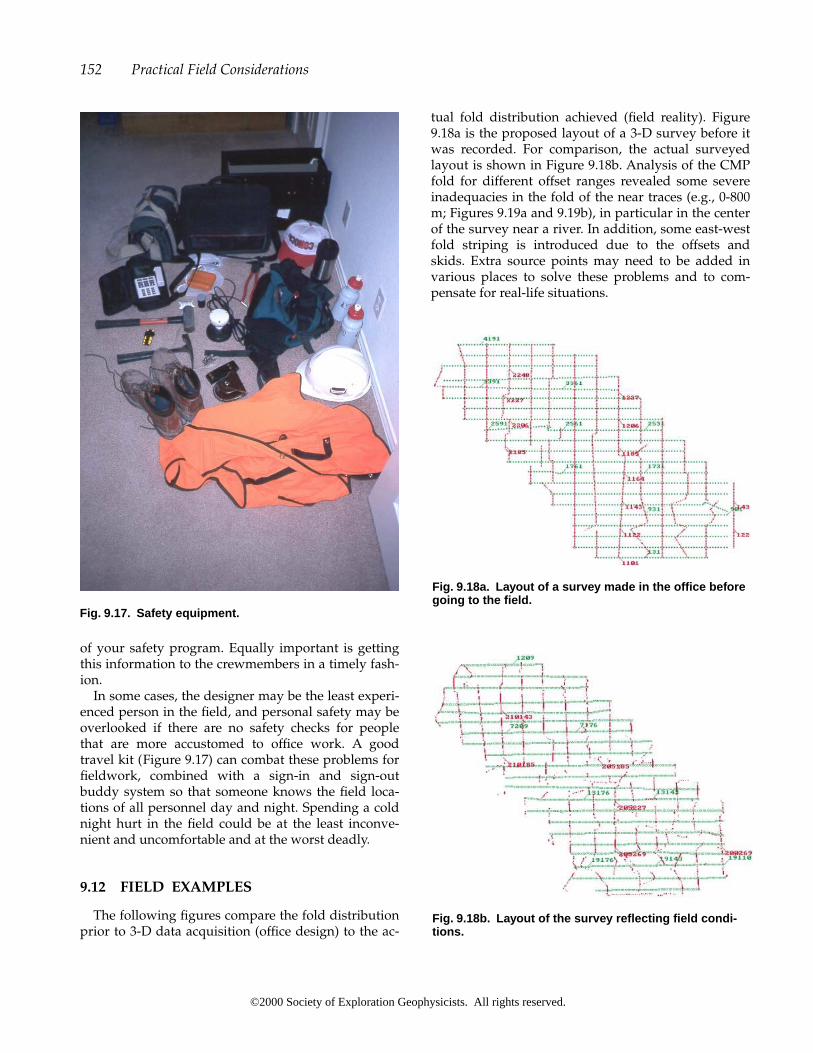
of your safety program. Equally important is gettingthis information to the crewmembers in a timely fash-ion.
In some cases, the designer may be the least experi-enced person in the field, and personal safety may beoverlooked if there are no safety checks for peoplethat are more accustomed to office work. A goodtravel kit (Figure 9.17) can combat these problems forfieldwork, combined with a sign-in and sign-outbuddy system so that someone knows the field loca-tions of all personnel day and night. Spending a coldnight hurt in the field could be at the least inconve-nient and uncomfortable and at the worst deadly.
9.12 FIELD EXAMPLES
The following figures compare the fold distributionprior to 3-D data acquisition (office design) to the ac-
tual fold distribution achieved (field reality). Figure9.18a is the proposed layout of a 3-D survey before itwas recorded. For comparison, the actual surveyedlayout is shown in Figure 9.18b. Analysis of the CMPfold for different offset ranges revealed some severeinadequacies in the fold of the near traces (e.g., 0-800m; Figures 9.19a and 9.19b), in particular in the centerof the survey near a river. In addition, some east-westfold striping is introduced due to the offsets andskids. Extra source points may need to be added invarious places to solve these problems and to com-pensate for real-life situations.
152 Practical Field Considerations
Fig. 9.17. Safety equipment.
Fig. 9.18a. Layout of a survey made in the office beforegoing to the field.
Fig. 9.18b. Layout of the survey reflecting field condi-tions.
©2000 Society of Exploration Geophysicists. All rights reserved.

9.13 FIELD QC (DATA)
In 3-D seismic surveys, the volume of data can beoverwhelming. It is essential to have methods thatquickly identify errors and/or bad data. Modern fieldQC uses seismic trace attributes (energy levels withinspecified windows, energy decay factors, first arrivaltimes) in combination with survey information (shotand receiver positions) to create new quality controlmeasurements and displays. Such QC displays canusually pinpoint location errors and other problems atboth shot and receiver positions.
There are three basic reasons to process data in thefield:
1. To verify accuracy of trace headers—3-D geome-try.
2. To generate quasi-real-time interpretable resultsfor modifying the field program or siting a well.
3. To enable fast-track processing in a remote data-processing center.
In-field quality control processing verifies the fol-lowing:
positional data qualityseismic data qualityseismic/positional data relationship
The most important item is the seismic/positionaldata relationship. By examining the relationship be-tween seismic data and the position in which the en-ergy was initiated (source point), the subsurface ittraveled through (CMP), and its recording position(field station or receiver), one can determine the accu-racy of the position data and the quality of the seismicdata. Those relationships help determine the first-break times, trace to trace variations in amplitude,and the expected spatial continuity of data attributessuch as exponential amplitude decay.
9.13.1 Positional Data Quality
To verify position data, one can perform conven-tional offline geodetic QC, but the most usefulmethod is to overlay final survey coordinates onto amap or image (TIFF or DXF files). The visual tie be-tween shot and receiver positions and the actualground is a compelling verification of accuracy.
9.13.2 Seismic Data Quality
A display of seismic data can reveal much aboutpotential position errors and answer questions, suchas:
Do the first breaks look as expected (in comparisonto a theoretical first-break template overlay)?
Are the number of shots and number of traces pershot as expected?
Is the data quality as expected (are there any reflections)?
Is the noise level acceptable (are there a lot of badtraces/receivers)?
9.13 Field QC (Data) 153
Fig. 9.19a. Office design with short offsets.
Fig. 9.19b. Field reality with short offsets.
©2000 Society of Exploration Geophysicists. All rights reserved.

9.13.3 Verify Seismic/Positional DataRelationship
The relationship between shot, CMP, and receiverpositions dictates how the data appear. In otherwords, the first breaks appear at a certain time andthe amplitude of the data follows the laws of spheri-cal divergence and inelastic attenuation. A semirigor-ous method includes the verification of shot, receiver,and CMP information, and the continuity of trace at-tributes to verify relationships (data and position).
The seismic data trace attributes may be chosenfrom the following:
• The first-break times are related to the horizontaldistance between shot and receiver. As a result, onecan verify relative position correctness.
• The average amplitude within a window around thefirst breaks and within the data indicates how muchspherical divergence there has been. Consequently,one can exploit the relation between amplitude andshot/receiver offset. This can verify first break in-formation in the case of bad picks or no picks.
• The amplitude decay factor indicates the pathtaken by the energy traveling from shot to receiver.This attribute is therefore related to some area ofthe subsurface. Such an attribute can be used toverify correctness of global position by studying itsspatial continuity.
• The frequency at maximum amplitude is again re-lated to the subsurface path. It is, however, mostuseful in detecting bad traces. Frequency is gener-ally the same for all good traces but can be quitedifferent on noisy traces (often associated with a re-ceiver station).
• The signal-to-noise ratio is calculated as the ratio ofrms amplitude within a window ahead of the firstbreaks (the “noise” window) to the rms amplitudein a window that includes signal within the data.The signal-to-noise ratio can be affected by manyfactors such as surface conditions, offset, groundroll and other linear shot noise, random noise, andbad channels.Other attributes can be similarly classified accord-
ing to their use in verifying or determining shot andreceiver position.
Relationship Diagnostics for Shot/Receivers
In a rigorous QC procedure, a map of shots and re-ceivers may display the minimum, maximum, and av-erage (mean) of these items:
elevation of shots and receiversshot and receiver line numbers
shotpoint and field station numbersshot, receiver, and CMP folddepth of shot, uphole times, datum elevationmean rms amplitudesamplitude decay factorsmaximum frequencysignal-to-noise ratio
Definition of amplitude decay:
A single parameter a can be used to define the ex-ponential decay of a data trace by a least-squares fit ofthe curve e at to the peaks of the absolute trace ampli-tudes (Figure 9.20). This parameter is directly relatedto the energy travel path, and therefore to subsurfacegeology. This parameter should show spatial varia-tions that have a logical relationship to geology.
Definition of trace statistics:
A single parameter, “maximum frequency,” can bedefined for each trace. This is the frequency of themaximum amplitude of a spectrum derived fromsome window of the data (Figure 9.21).
Relationship Diagnostics Shots/Receivers
The following header word values for each sourcepoint might be displayed on a map of sources and re-ceivers.
Xmid , Ymid
shot receiver azimuthrms amplitudefirst-break times
Relationship Diagnostics Sources/Receivers:
Other relationships are examined through the useof graphs and cross-plots, such as shotpoint number,
154 Practical Field Considerations
Fig. 9.20. Definition of the amplitude decay parameter.
©2000 Society of Exploration Geophysicists. All rights reserved.

offsets for each trace, and the rms amplitude of a win-dow around the first breaks. An excellent agreementbetween the offset and amplitude is a further confir-mation of relative position accuracy.
Predicting source locations from first-break times ateach receiver should be plotted as a check. The sourcelocation can be predicted based on the knowledge of all receiver coordinates for each shot and the first-break times. In Figure 9.22, two small arrows onthe right-hand side indicate source points that shouldbe moved. In other words, the source point at the“tail” of the arrow should be moved to the “head” ofthe arrow to satisfy the combination of first-breakpick times and source location. The maximum ampli-tude times appear to be centered around the head of
the arrow, which indicates the correctness of the prediction.
Predictions can be repeated based on rms ampli-tudes of a window over the first arrivals. In general,this is not as accurate as first-break times but can helpto confirm the prediction. The receiver position canalso be predicted based on the knowledge of allsource coordinates (source points fired into each re-ceiver) and the first-break time.
Other QC diagnostics:
Many QC diagnostics can further confirm (or deny)the accuracy of geometry information. Some of themost useful and enduring of these are:
• 100% displays• field stacks• raw record displays • use of in-line/cross-line displays• time slice
The main use of each is to emphasize spatial conti-nuity of data attributes. Discontinuities generally in-dicate the presence of a survey or data-coordinate error.
Further QC diagnostics may also be used to checkthe integrity of the seismic data itself. Such diagnos-tics tell more about the recoverable signal contentthan any relationship to position information. Suchdiagnostics may include:
• amplitude spectra• filter panel plots (define signal bandwidth)• deconvolution panels• Farr diagrams [apply largest minimum offset
(LMO) to each shot and plot first-breaks in cas-caded format at their surface position]
• f-k spectra
Field QC can establish the accuracy of the surveygeometry and offers information about the signal con-tent of the data. In general field QC can identify,quantify, and assist the following:
• position/seismic attribute relationships• list of dead/reverse traces (shots, receivers, chan-
nels)• data preprocessing• velocity analysis• processing trials (establish sequence and parame-
ters)• list of unusual data aspects
Field QC can enable fast-track data processing. Allof these items contribute to faster throughput in the
9.13 Field QC (Data) 155
Fig. 9.21. Definition of the maximum frequency parame-ter.
Fig. 9.22. Prediction of shot locations from first breaktimes and verification using the times of maximum am-plitude for each trace.
©2000 Society of Exploration Geophysicists. All rights reserved.

processing center and to a more successful result fromthe 3-D survey.
Chapter 9 Quiz
1. How does a final plan differ from a preplot?2. Describe the essential elements of a script file.
3. Does roll-on and roll-off result in higher or lowerfold?
4. When are snaking (movement of sources acrossmultiple receiver line intervals) and ping-pong-ing used?
©2000 Society of Exploration Geophysicists. All rights reserved.

This chapter is not intended to be a thorough treat-ment of seismic data processing; the topic of data pro-cessing is thoroughly discussed by Yilmaz (1987).Rather, this chapter introduces and briefly discussessome processing issues that are closely related to 3-Dacquisition.
10.1 PROCESSING
It is of utmost importance to find a processor whocan efficiently conduct the required 3-D data analyses.Quality control (QC) is so important that at least oneperson needs to be committed to examining theprogress of the processing at numerous stagesthroughout the 3-D project. Larger companies mayhave a dedicated processing QC group rather thanhaving the interpreter be responsible for the processingQC. The best processor and the best QC person need tobe brought together to achieve optimal data quality.
Field processing systems are now so small thatmany acquisition companies have full processing ca-pabilities on the job site. The client has to evaluate theadvantages of faster data-processing turnaround withthe additional costs involved with such amenities(Duncan et al., 1996). For larger 3-D data sets, one hasto make sure that the field processing center can effec-tively carry out the tasks. In such cases, the field pro-cessing center may be used only for quality control,data editing, or first-break picking. The quality con-trol must be just as efficient as if the data wereprocessed in an office environment.
Preparation of the 3-D geometry itself is by far thelargest task in processing. Some processors estimate atleast 50%—and some up to 70%—of the total timespent in processing concentrates on 3-D geometry.Good QC tools are essential to the verification of the3-D geometry.
To avoid surprises, the processing stream needs tobe defined and a pricing schedule established beforeprocessing commences. Most companies prefer onlytape or CD-ROM copies for workstation manipulationof the data. However, at times it is necessary to per-form a quick check on some aspect of the data, and, insuch cases, some form of hard copy might be prefer-able. Selected portions of the 3-D data volume can bedisplayed on paper or reproducible film. Time slicesof data volumes at various stages of processing are ef-fective quality control tools. It is essential to overlaythe recording geometry on these time slices to detectgeometry-induced artifacts (acquisition footprints).
10.2 PROCESSING STREAM
Processing skills, experience, and the appropriate-ness of a given software package to process seismicdata from a specific geographic area are not uniformfrom one processing company to another. Therefore itmay be appropriate to have the 3-D data processed byseveral processing contractors as part of a risk reduc-tion procedure (Bouska, 1998b).
A typical data-processing stream is shown in Table10.1. The first group of items represents a basic pro-cessing stream for which turnkey prices are often pro-vided. The second list of items represents possible in-termediate add-on services for which unit prices canbe quoted. The last three groups are minimum deliv-erable products (paper, film, and tape) one should ex-pect to receive as part of the turnkey price. Some con-tractors may offer additional add-on services on aprice-per-unit basis.
The importance of correct survey information needsto be emphasized. A change as small as 15 m (50 ft) inaccurate line or point position can play havoc withthe processing for an entire 3-D. In the absence of
157
10Processing
©2000 Society of Exploration Geophysicists. All rights reserved.

correct survey information, the processor can still usefirst arrival times to place the source points in theircorrect spatial position. However, this is a time-con-suming task, which is best avoided.
A set of standard film displays for 3-D surveys canbe helpful even when workstations are used for theinterpretation. It is recommended that regional dis-plays of every tenth line be available, as well as zone-of-interest plots for every line or every second line, toretain detailed information in hard-copy form thatwill be needed for picking well locations. All of these
displays should be made for both polarities in bothdirections.
10.3 REFRACTION STATICS
Source-to-receiver times (first-break times) are es-sential to solve for refraction statics. If such measure-ments are not present in both in-line and cross-line di-rections there is no tie between lines or portions oflines (as is the case for narrow receiver patches).
Short offsets are needed for shallow refractors.Therefore the receiver line spacing must be smallenough to adequately sample shallow refractors be-cause a small Xmin is necessary to define the first re-fractor interface. Note that all cross-line and in-linecoupling is lost when the receiver line interval isgreater than the offset needed to get refraction infor-mation from the shallowest refractor. This offset isshown as X1 in Figure 10.1.
The equations used to solve for the velocity of eachrefractor involve source-receiver pairs and their mid-points. In any regular geometry (straight, brick,zigzag, etc.), these equations are not coupled (see Re-flection Statics below). The only way to solve such un-coupled equations is to use a velocity smoother overseveral CMPs. This smoothing technique means thatundetermined long-wavelength errors will be presentin the velocities and may appear in either the sourceor receiver delays.
The use of a narrow receiver patch also introducesproblems. It is important that the patch be wideenough to collect cross-line measurements for deeprefractors. Otherwise, there are few direct measure-ments of deep refractors from any given source point
158 Processing
Table 10.1. Processing requirements.
Processing sequence (turnkey price):Demultiplex and edit field dataGain recoveryInstrument and geophone dephasingGeometry and refraction statics analysisDeconvolution and filter testsSurface-consistent deconvolution and scalingBrute stackVelocity analysisAutomatic surface consistent staticsIntermediate stacksFinal velocity analysis3-D trim stack with final staticsFX-decon3-D migration after stack, one-pass
Options possible (price per unit):3-D interpolationBin-borrowing or mixingRebinningf-k noise attenuationDMOMultiple attenuation (e.g., Radon transform)Depth migration—mainly after stackPrestack time or depth migration
Deliverables (paper):Selected shot records, before and after NMOCommon-offset stacks with mute displaysDecon testsNarrow and broad-band filter testsBrute stackVelocity analysis displays (e.g., semblance)Intermediate stackFinal stackMigration
Deliverables (film):Map of source and receiver locationsSubsurface bin and coverage mapsMigration (e.g., every tenth line, both polarities, both di-
rections)Deliverables (SEG-Y tape):
FX-decon—unfiltered and filteredMigration—unfiltered and filtered
Fig. 10.1. Refraction criterion—plan view and sectionview showing relationship between line spacings andrefraction statics. Compare with Figure 2.17b.
©2000 Society of Exploration Geophysicists. All rights reserved.

to its associated receivers in the cross-line direction.The variations of such refractors in the cross-line di-rection can be determined only by combining varia-tions from a receiver line to an immediate neighbor-ing receiver line. Such a combination will almostcertainly be prone to error. It is therefore essential tohave in-line and cross-line offsets along both sourceand receiver line directions that define all near-surfacelow-velocity layers.
10.4 VELOCITY ANALYSIS
A stacking velocity analysis should be performed asoften as necessary to provide a good velocity field. Attimes, velocity analyses are done every 500 m in bothdirections to create a grid of velocity control points.On small surveys or surveys with more geologicalcomplexity, one may wish to have a velocity analysisgrid point at every line intersection. Vertical travel-time calculations are based on straight raypath theoryand constant velocity assumptions. Semblance analy-sis is used to estimate maximum coherence along amoveout curve, which then defines the stacking ve-locity function. Semblance analysis should not beused when the interpreter is expecting AVO effects,because one of the basic assumptions in semblanceanalysis is that the signal amplitude does not varywith offset.
Sometimes a super bin, i.e., several bins grouped to-gether, is used to create a good mix of offsets. All off-sets should be grouped by azimuth because velocity
analysis is a directional property in a 3-D survey. Eachset of offsets in each azimuth range must adequatelydefine normal moveout (NMO) curves, which meansthe delta-t change should exceed one wavelength(Figure 10.2a). Care must be exercised to choose a su-per bin that is small enough to not smear geologicalstructures (Figure 10.2b).
The velocity resolution of each CMP bin in a realsurvey can be calculated by creating a synthetic eventwith a specified velocity and time, and then stackingthe synthetic data at different velocities. An exampleof such a synthetic event ray-traced for an actual off-set mix across several CMPs of a real 3-D survey isshown in Figure 10.3. Several synthetic CMP gathertraces before NMO are shown in Figure 10.3a. The re-sult of stacking one of these gathers (traces belongingto one CMP) at many different velocities is shown inthe bottom display (Figure 10.3b). The correct velocityis reasonably obvious (approximately CVS trace 201),but a small error in picking is still quite possible, par-ticularly in real data.
This fact is further borne out by looking at a sem-blance analysis of the same data in Figure 10.4. Theoffsets that record the synthetic data as a flat event arenot regular. As a result, the pick for the correct veloc-ity cannot be made with total accuracy. On a com-puter-driven semblance plot, it was possible to pick avelocity 50 m/s either side of the correct answer andstill satisfy the criterion of picking the maximum am-plitude in the semblance. The picks can be made onthe first peak, the trough, or the second peak. In thiscase, the trough is picked. In real data there is, ofcourse, no such certainty. This velocity picking varia-tion (� 50 m/s in this example) is referred to as thevelocity resolution.
Figure 10.5 defines the velocity resolution graphi-cally. This plot shows the maximum amplitude of thestack trace as a function of the NMO velocity that wasapplied before stack. At the correct NMO velocity, theamplitude of the stack trace achieves a maximumvalue. There is some uncertainty as to exactly wherethis maximum amplitude occurs. Obviously the am-plitude of a stack trace is much lower when the wrongvelocity is used, whether the velocity is too high ortoo low. The breadth of the velocity versus amplitudecurve at this level (e.g., 3% off the peak) is a finitequantity in velocity units that is defined as the velocityresolution. In effect, velocity resolution is a singlequantity that expresses the ability of the offset mix ina CMP bin to correctly focus a specified target. Thisvelocity measure is affected by the mix of offsets andis in fact a powerful indicator of good and bad offsetdistribution.
10.4 Velocity Analysis 159
Fig. 10.2. Velocity analysis concepts for: a. NMO and b.super bins.
©2000 Society of Exploration Geophysicists. All rights reserved.
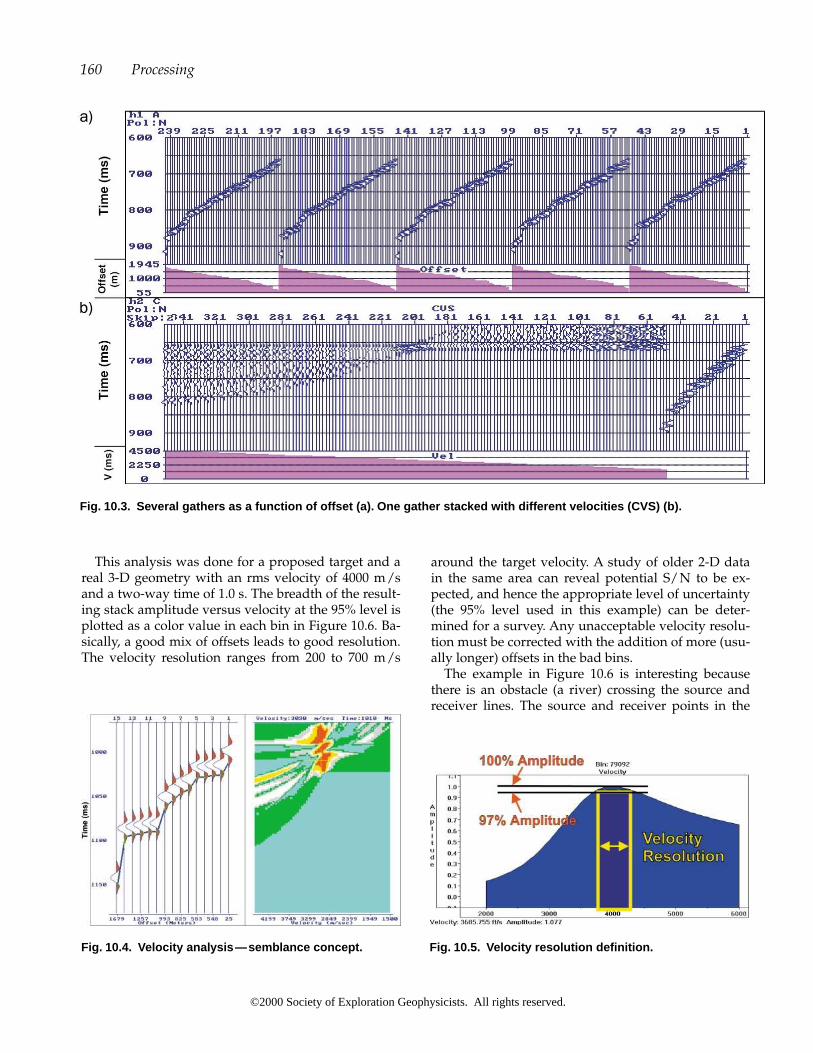
This analysis was done for a proposed target and areal 3-D geometry with an rms velocity of 4000 m/sand a two-way time of 1.0 s. The breadth of the result-ing stack amplitude versus velocity at the 95% level isplotted as a color value in each bin in Figure 10.6. Ba-sically, a good mix of offsets leads to good resolution.The velocity resolution ranges from 200 to 700 m/s
around the target velocity. A study of older 2-D datain the same area can reveal potential S/N to be ex-pected, and hence the appropriate level of uncertainty(the 95% level used in this example) can be deter-mined for a survey. Any unacceptable velocity resolu-tion must be corrected with the addition of more (usu-ally longer) offsets in the bad bins.
The example in Figure 10.6 is interesting becausethere is an obstacle (a river) crossing the source andreceiver lines. The source and receiver points in the
160 Processing
Fig. 10.3. Several gathers as a function of offset (a). One gather stacked with different velocities (CVS) (b).
Fig. 10.5. Velocity resolution definition.Fig. 10.4. Velocity analysis—semblance concept.
©2000 Society of Exploration Geophysicists. All rights reserved.

river were excluded. Thus the offset mix in CMP binsnear the river was affected. The effect of the river ismirrored in bins that are parallel to the river and posi-tioned up to 200 m on either side. In this zone of bins,there is a higher value of velocity uncertainty, indicat-ing that a seismic data processor must take care in se-lecting zones of CMPs for velocity analysis, especiallynear excluded areas in the 3-D survey. In the bins thatfall under the location of the river, the velocity resolu-tion is improved because there are relatively more faroffsets that help improve the accuracy of the velocitydetermination.
10.5 REFLECTION STATICS
In the processing step of reflection statics, the tracesof each, or possibly many, bins are summed to form astable and representative pilot trace for each CMP bin.Crosscorrelation of the individual traces that enterinto a stack for a particular bin with the pilot trace forthat bin determines the static time shift values to beapplied to each trace. Matrix calculations separate thestatic corrections for each source and receiver locationto create what is commonly called a surface-consistentsolution.
Statics coupling (Wiggins et al., 1976) implies thateach receiver position is fired into by many sourcepoints and vice versa. Crosscorrelation methods de-tect time differences between adjacent receivers andadjacent source points. These time differences, whenmultiplied by the inverse of the geometry matrix, pro-vide the surface-consistent static values at each re-ceiver and source position. If the inverse of the geom-etry has holes in it, then the statics are undetermined
for certain spatial wavelengths. The absolute staticvalues can be thought of as being composed of a sumof different spatial wavelengths.
The occurrence of holes usually means that thegeometry matrix is under-determined; that is, equa-tions that define the statics for some receivers orsource points are missing. In other words, there aretoo few equations to overcome potential picking er-rors (Figure 10.7). The number of equations requiredfor surface-consistent static calculations is controlledby the number of source-receiver pairs that create re-flection points in each bin.
Figure 10.8 illustrates the different source-receiverpairs that contribute to neighboring CMP bins. Thisorthogonal survey example demonstrates that ifsource points 1, 5, 9, . . . , contribute to one CMPbin, then source points 2, 6, 10, . . . , contribute tothe next CMP bin, and source points 3, 7, 11, . . . , tothe bin after that. This means that in all the equationsfor each source-receiver pair, there will be no equa-tions that link the shot static for source point 1 to thatfor source point 2, or the shot static for source point 3to that for source point 4. Instead, source point 1 is
10.5 Reflection Statics 161
Fig. 10.6. Distrib ution of velocity resolution over an ex-clusion zone (river).
Fig. 10.7. Reflection statics equation (surface consis-tent).
Fig. 10.8. Reflection statics—coupling.
©2000 Society of Exploration Geophysicists. All rights reserved.

linked to source point 5 (and 9, 13, etc.). In this casethere are four families of equations that are not con-nected to each other. The ratios of RLI/SI and SLI/RIdetermine the number of families for receiver andsource static solutions.
It is now known (Wisecup, 1994) that all regularlyspaced straight-line geometries (brick, zig-zag, etc.)are uncoupled for statics (except the fully populated3-D). That is, there is more than one independent so-lution for source and receiver statics. To tie indepen-dent solutions together, Wisecup (1994) suggests theuse of smoothers in the structure term. This normallygives reasonable answers (no cross-line “jitter”), butcan leave errors in the long-wavelength statics andmay not adequately resolve a structural anomaly. Inthe Flexi-Bin® design, all sources and all receivers arecoupled, because of the nonrepetitive nature of therelative positions of sources and receivers at the lineintersections; this causes the interleaving of the cross-spreads (see Chapter 5).
In the limit, a 3-D survey can be shot as a series of2-D lines. In such a case there is no coupling of solu-tions between adjacent lines; hence each solution canbe independently high or low. As more receiver linesare added to the patch, an element of cross-line cou-pling is introduced, and the solutions exhibit morecontinuity in the cross-line direction. Note that thefull swath roll (see Chapter 9) is uncoupled fromswath to swath, except through the source points.Hence if there are any appreciable statics (more than10 ms), this geometry should not be used because shotstatics are not repeatable from one swath to the next.
Statics coupling can be assured by creating irregu-larity in the source, receiver, or line spacings (Figure10.9). Another option is to add source lines in the re-ceiver line direction and receiver lines in the source
line direction. It should be noted that a geometry thatis good for statics may not be optimum for imaging. Inother words, near-surface imaging, which is what stat-ics offer, may not be the ultimate objective, but rather a3-D subsurface image is sought. Compromises, there-fore, must always favor the subsurface targets. A com-puter program should be used to check each layout.
10.6 DIP MOVE-OUT
While NMO corrects for the time delay on an offsettrace by moving the amplitudes to earlier times on thetrace, DMO moves the data up-dip to the correct posi-tion where a zero-offset trace would record a dippingreflector (Figure 10.10). Migration then moves the en-ergy to the correct horizontal and vertical subsurfacelocation. Russell (1998) provides a good summary ex-ercise for the DMO process.
DMO is a dip-specific application of prestack par-tial migration followed by NMO and stack. Hale(1984) discusses the process in detail. Constant-veloc-ity DMO is the most commonly applied method.Time-variant DMO has been described by Meinardusand Schleicher (1991).
The DMO ellipse has the biggest effect on data atshallow times and at far offsets. Varying surfacegeometry may introduce amplitude anomalies due todifferent offset and azimuth mixes, that may or may
162 Processing
Fig. 10.9. Irregular geometry provides coupling (artifi-cial example).
Fig. 10.10. Data movement during NMO, DMO, and mi-gration (after Sheriff, 1991).
©2000 Society of Exploration Geophysicists. All rights reserved.

not be compensated for in processing. Three-dimen-sional DMO needs as many offsets as possible in eachazimuth range to form the reflections by constructiveinterference. Otherwise, imperfect image reconstruc-tion occurs. This construction of offset sections can bedifficult in 3-D surveys because of midpoint scatteringand source-receiver azimuth variations. Therefore, notall 3-D designs lend themselves to the successful ap-plication of DMO.
Let H be the source-receiver offset, V the averagevelocity, and t the time of interest. Then the energy attime t in a CMP bin is derived from all source-receiverpairs that cross the bin and whose midpoints arewithin of the bin center as shown in Figure 10.11 (Deregowski, 1982). Fold and the number of unique offsets in each bin after DMO attime t are good measures of the DMO response. FromFigure 10.11,
(10.1)
Example: if V � 3000 m/s H � 1000 m t � 1.0 s
DMO radius � 170 m (or about 7 bins if B � 25 m)
or if V � 10 000 ft/s H � 3000 ft t � 1.0 s
DMO radius � 450 ft (or about 4 bins if B � 110 ft)
In other words, all traces that have an offset of 1000m (3000 ft), a source-receiver azimuth that passesthrough a central bin, and a midpoint that is within170 m (450 ft) of that central bin, will contribute en-
DMO radius �H 2
2Vt.
H 2 � (2 � V � t)
ergy to the central bin. Note that a 5° dipping reflectorin this situation has its energy shifted a horizontal dis-tance of 15 m as defined by the equation:
(10.2)
where � is the reflector dip.The central sample in Figure 10.12 is created from
many other traces that provide contributing energy.The farther away a trace is from the center trace, thesteeper the dip of the energy that contributes to the center sample. Constructive interference ensuresthat dips are reconstructed (imaged) at their properzero-offset position where stacking takes place ratherthan at the CMP position. Migration after stack thenmoves the dips to their correct geologic position(CDP). If traces are missing, the constructive interfer-ence is disrupted. This effect is usually referred to asgeometry imprinting (or acquisition footprint, seeSection 10.8). Poor geometry design may create holesin the offset plane, and the lack of certain offsets in aregular pattern may impede the constructive interfer-ence process for certain dips. A sample at time t is re-constructed as:
sample at time t � � {all offset traces [� all dips]}� Dip 1 traces (� all offsets)
� Dip 2 traces (� all offsets)� Dip 3 traces (� all offsets) � . . . .
Missing traces in the common-offset panel will notcontribute to certain dips. The number of live tracescontributing to each dip range are counted. The sumof the first and second moments of the DMO opera-tors at each CMP position for each offset range canalso be used (Jakubowicz, 1990; Beasley, 1993).
H 2
V � t � sin � � cos �,
10.6 Dip Move-out 163
Fig. 10.11. DMO contributions to a bin. Fig. 10.12. DMO—dip decomposition.
©2000 Society of Exploration Geophysicists. All rights reserved.
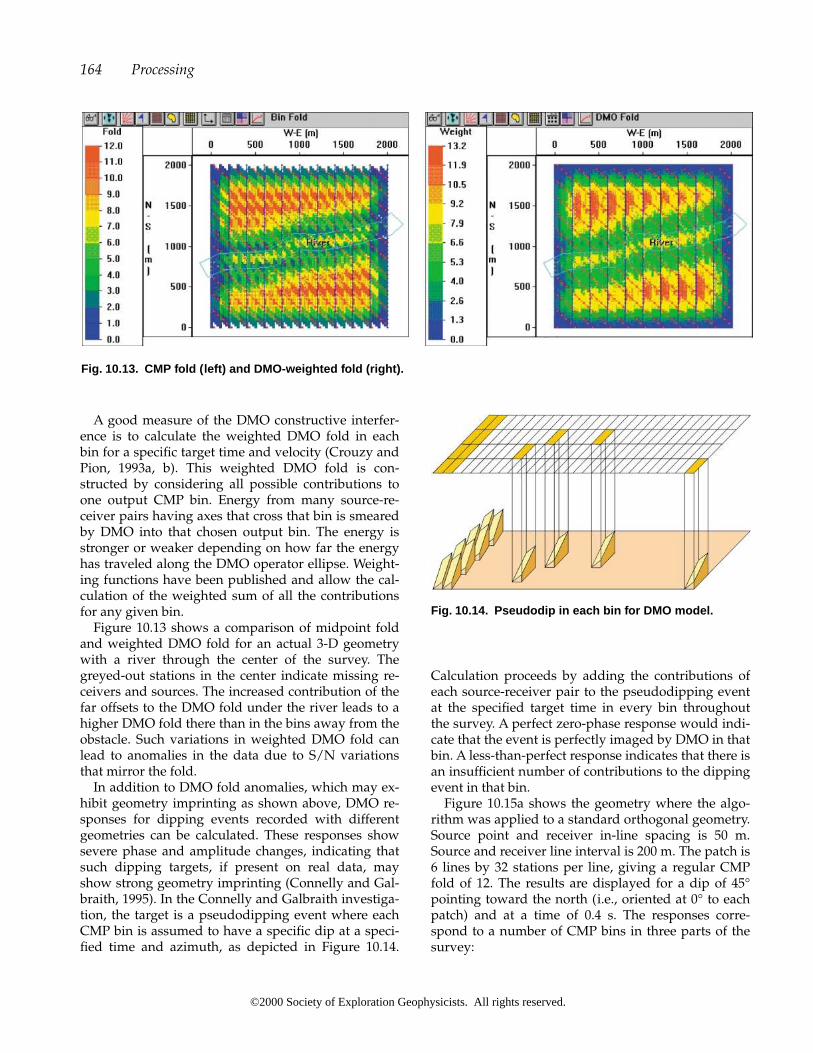
A good measure of the DMO constructive interfer-ence is to calculate the weighted DMO fold in eachbin for a specific target time and velocity (Crouzy andPion, 1993a, b). This weighted DMO fold is con-structed by considering all possible contributions toone output CMP bin. Energy from many source-re-ceiver pairs having axes that cross that bin is smearedby DMO into that chosen output bin. The energy isstronger or weaker depending on how far the energyhas traveled along the DMO operator ellipse. Weight-ing functions have been published and allow the cal-culation of the weighted sum of all the contributionsfor any given bin.
Figure 10.13 shows a comparison of midpoint foldand weighted DMO fold for an actual 3-D geometrywith a river through the center of the survey. Thegreyed-out stations in the center indicate missing re-ceivers and sources. The increased contribution of thefar offsets to the DMO fold under the river leads to ahigher DMO fold there than in the bins away from theobstacle. Such variations in weighted DMO fold canlead to anomalies in the data due to S/N variationsthat mirror the fold.
In addition to DMO fold anomalies, which may ex-hibit geometry imprinting as shown above, DMO re-sponses for dipping events recorded with differentgeometries can be calculated. These responses showsevere phase and amplitude changes, indicating thatsuch dipping targets, if present on real data, mayshow strong geometry imprinting (Connelly and Gal-braith, 1995). In the Connelly and Galbraith investiga-tion, the target is a pseudodipping event where eachCMP bin is assumed to have a specific dip at a speci-fied time and azimuth, as depicted in Figure 10.14.
Calculation proceeds by adding the contributions ofeach source-receiver pair to the pseudodipping eventat the specified target time in every bin throughoutthe survey. A perfect zero-phase response would indi-cate that the event is perfectly imaged by DMO in thatbin. A less-than-perfect response indicates that there isan insufficient number of contributions to the dippingevent in that bin.
Figure 10.15a shows the geometry where the algo-rithm was applied to a standard orthogonal geometry.Source point and receiver in-line spacing is 50 m.Source and receiver line interval is 200 m. The patch is6 lines by 32 stations per line, giving a regular CMPfold of 12. The results are displayed for a dip of 45°pointing toward the north (i.e., oriented at 0° to eachpatch) and at a time of 0.4 s. The responses corre-spond to a number of CMP bins in three parts of thesurvey:
164 Processing
Fig. 10.13. CMP fold (left) and DMO-weighted fold (right).
Fig. 10.14. Pseudodip in each bin for DMO model.
©2000 Society of Exploration Geophysicists. All rights reserved.

1) along the central receiver line (Figure 10.15b),2) along the central source line (Figure 10.15c), and3) an areal view of the center of the survey (Figure
10.15d).
There are significant amplitude and phase changesindicating that the output of DMO applied to realseismic data collected with this geometry would havea strong geometry imprint for any northerly dippingevents of 45° close to a time of 0.4 s. The imprint inthis case is mostly due to the excluded shots and re-ceivers, although it is also possible to see a variationin DMO response at each shot and/or receiver line in-tersection.
Other examples with different geometry and foldindicate similar results. In general, there are problemswith steeper dips at shallow times and with dips
across narrow patches. These imaging problems pointto a need to either:
a) calculate some form of amplitude and phasecompensation (inverse DMO operator), or
b) redesign the acquisition geometry to im-prove the DMO output contributions in all bins for the desired target dip and time. A general rule for areal (land) geometries is to not use narrow patches for DMO applications.
Although these studies specifically involved DMO,it is likely that other imaging techniques (e.g.,prestack time or depth migration) suffer from similarproblems, namely, insufficient in-phase cross-line con-tributions that lead to a poorly focused image.
10.6 Dip Move-out 165
Fig. 10.15. a. 3-D survey showing DMO analysis bins. DMO model response: b. along a portion of the central receiverline, c. along the central source line, d. for all bins in the center of the survey.
©2000 Society of Exploration Geophysicists. All rights reserved.
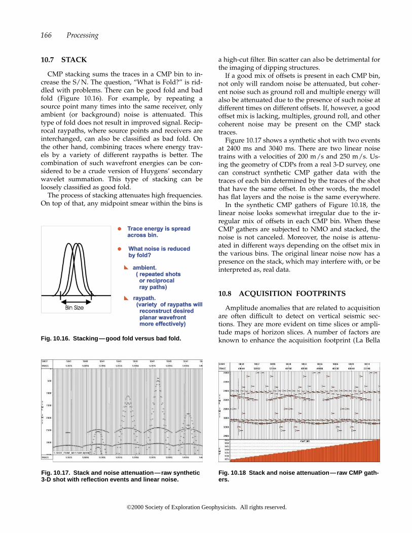
10.7 STACK
CMP stacking sums the traces in a CMP bin to in-crease the S/N. The question, “What is Fold?” is rid-dled with problems. There can be good fold and badfold (Figure 10.16). For example, by repeating asource point many times into the same receiver, onlyambient (or background) noise is attenuated. Thistype of fold does not result in improved signal. Recip-rocal raypaths, where source points and receivers areinterchanged, can also be classified as bad fold. Onthe other hand, combining traces where energy trav-els by a variety of different raypaths is better. Thecombination of such wavefront energies can be con-sidered to be a crude version of Huygens’ secondarywavelet summation. This type of stacking can beloosely classified as good fold.
The process of stacking attenuates high frequencies.On top of that, any midpoint smear within the bins is
a high-cut filter. Bin scatter can also be detrimental forthe imaging of dipping structures.
If a good mix of offsets is present in each CMP bin,not only will random noise be attenuated, but coher-ent noise such as ground roll and multiple energy willalso be attenuated due to the presence of such noise atdifferent times on different offsets. If, however, a goodoffset mix is lacking, multiples, ground roll, and othercoherent noise may be present on the CMP stacktraces.
Figure 10.17 shows a synthetic shot with two eventsat 2400 ms and 3040 ms. There are two linear noisetrains with a velocities of 200 m/s and 250 m/s. Us-ing the geometry of CDPs from a real 3-D survey, onecan construct synthetic CMP gather data with thetraces of each bin determined by the traces of the shotthat have the same offset. In other words, the modelhas flat layers and the noise is the same everywhere.
In the synthetic CMP gathers of Figure 10.18, thelinear noise looks somewhat irregular due to the ir-regular mix of offsets in each CMP bin. When theseCMP gathers are subjected to NMO and stacked, thenoise is not canceled. Moreover, the noise is attenu-ated in different ways depending on the offset mix inthe various bins. The original linear noise now has apresence on the stack, which may interfere with, or beinterpreted as, real data.
10.8 ACQUISITION FOOTPRINTS
Amplitude anomalies that are related to acquisitionare often difficult to detect on vertical seismic sec-tions. They are more evident on time slices or ampli-tude maps of horizon slices. A number of factors areknown to enhance the acquisition footprint (La Bella
166 Processing
Fig. 10.16. Stacking— good fold versus bad fold.
Fig. 10.17. Stack and noise attenuation—raw synthetic3-D shot with reflection events and linear noise.
Fig. 10.18 Stack and noise attenuation—raw CMP gath-ers.
©2000 Society of Exploration Geophysicists. All rights reserved.

et al., 1998). It is desirable to reduce this footprint asmuch as possible in the acquisition process. Acquisi-tion footprints can arise from a variety of causes, suchas:
• changes in the signal-to-noise ratio caused by bin-to-bin fold variations
• linear noise stacking in different ways because ofvariation in offset distribution
• multiple energy remaining after stack because ofvariation in offset and azimuth distribution
• azimuth and/or offset polarization• DMO failing to create constructive interference due
to missing offsets in some bins• backscatter noise combining in different ways in
neighboring bins as a result of azimuth and offsetdistribution variations
Figure 10.19a shows a CMP stack for several in-lines that are the equivalent of one “box.” Note theamplitude variations within each in-line, and the vari-ation from one in-line to the next. Figure 10.19b showsa graph of amplitude of the events at time 2400 msand time 3040 ms. Note the variations. The deeperevent is not as much affected by the noise imprint.Figure 10.19c shows the time slice of the event at time2400 ms with the true 3-D geometry superimposed.Note how the time slice amplitudes follow the 3-Dgeometry (source and receiver lines). Such noise rem-nants after stack are the most common form of “ac-quisition footprints” (geometry artifacts).
10.9 MIGRATION AND RANDOMSAMPLING
In recent years there have been many papers thatinvestigate how to use random sampling to reducemigration noise caused by coarse spatial sampling.Recommended readings are the papers published byVermeer (1996) and Schuster and Zhou (1996).
One of the more interesting illustrations is in Ver-meer (1996). Figure 10.20 displays the effect of sam-pling density for a horizontal event for five waveletsthat are formed by stacking along the diffractioncurve through the output sample position. The inputdata are a horizontal event with a wavelet corre-sponding to a vertical and horizontal resolution of12.5 m. The migration of the input data sampledevery 12.5 m produces a perfect result (left-mostwavelet). Increasing the spatial sampling to 33 m pro-duces a wavelet with precursor migration noise (mid-dle wavelet). Random samples with a mean value of
10.9 Migration and Random Sampling 167
Fig. 10.19a. CMP stack for several in-lines (equivalentof one “Box”).
Fig. 10.19b. Graph of amplitude of events at time �
2400 ms and time � 3040 ms.
Fig. 10.19c. Time slice of event at t � 2400 ms withgeometry superimposed.
©2000 Society of Exploration Geophysicists. All rights reserved.

33 m and a spread of 11 m either side of 33 m makeup the two right-most curves. Clearly the randomsampling has reduced the migration noise.
One should try to sample 3-D wavefields as finelyas possible to reduce migration noise for a wavelethaving the desired resolution. If fine sampling is im-possible, then random sampling can be effective. It ispossible to achieve somewhere near the desired reso-lution, and with less migration noise.
For 3-D data, the migration of regularly sampleddata already has an element of randomness, becausethe migration process is a function of the distancefrom input point to output point. These distances arenot regularly distributed in a 3-D geometry. EqualizedDMO may be applied to irregularly sampled 3-Ddata, requiring no particular acquisition geometryother than just source and receiver coordinates(Beasley and Mobley, 1998).
To achieve random sampling in the field, it is notnecessary to work at it. Normal bin to bin variations,of standard geometries (orthogonal, nonorthogonal,zig-zag, etc.) provide the necessary randomness.Moved sources and receivers create a further degreeof randomness.
10.10 MAKING ADJUSTMENTS FORDATA QUALITY
If data quality is unexpectedly low, the interpreter,in conjunction with the processor, has to evaluate thedata set to decide how to improve the signal-to-noiseratio. A multitude of possibilities exists. The easiestway to improve the S/N is to enlarge the bins. In atraditional 3-D survey this usually means doubling orquadrupling the bin size. The latter choice will in-crease the fold by a factor of four and double the S/N(Figure 10.21). If many offsets are redundant or the
offset mix is poor, the gain in S/N may not be as largeas expected. Note that linear source noise is non-Gaussian and therefore the S/N for that particularnoise will not improve with increasing fold.
Another option would be to perform some sort ofborrowing of information from neighboring binswhile retaining the original bin size. This borrowingcan be done depending on missing offsets or az-imuths in the center bin. These missing offsets can beadded from neighboring bins to increase the fold andtherefore improve the S/N. The only problem withthis approach is the large distance from one centralmidpoint to the next midpoint where the required in-formation is obtained. However, the data will appearsmoother, and in the case of extremely bad data, sucha strategy may make a 3-D survey interpretable. It isimportant to note that this kind of bin borrowing isexactly what DMO performs. Thus, if DMO is in-cluded in the seismic processing sequence, thereshould be no requirement for bin balancing/borrow-ing.
In extreme cases of bad data, a running mix of in-formation of neighboring bins will smooth the datapossibly to the point of making a correct interpreta-tion difficult, because the high frequency content mayhave been eliminated.
If the data quality is high, one may limit the re-quired offsets and azimuths to get a good representa-tion for each bin. If the fold distribution over the en-tire 3-D area can be smoothed, then the overall dataquality may be as good as or better than the originalfull-fold survey. In conventional 3-D surveys there isno method of decreasing the bin size to get a betterspatial resolution. The Flexi-Bin® approach distributes
168 Processing
Fig. 10.20. Eff ect of sampling density on migrated re-sponse (after Vermeer, 1996).
Fig. 10.21. Fold versus signal-to-noise ratio.
©2000 Society of Exploration Geophysicists. All rights reserved.

the midpoints within each bin in a prescribed manner.This distribution produces sub-bins that can besummed into bins with small bin size incrementsequal to the sub-bin dimensions rather than in multi-ples of the natural bin size. If the data quality is mar-ginal, the bin size can be increased; if the data qualityis high the bin size can be decreased (Section 5.7).
Bin rotation may be required to combine two ormore neighboring 3-Ds or if significant geological fea-tures are displaying unexpected trends (Figure 10.22).Such features could include channels, faults, and reeftrends. Figure 10.22a shows a 3-D layout following aneast-west fault direction based on geology only. The 3-D survey was acquired and revealed that the actualfault direction was northwest-southeast (Figure10.22b). The bins were rotated to have less bin linesaffected by the fault cut. Such bin rotation is difficult
to achieve with a conventional 3-D survey because ofthe central distribution of midpoints within each bin.In a survey where the midpoints are distributedwithin each bin (e.g., irregular line spacings, crookedline orientation, random, or Flexi-Bin®), such a changein bin orientation may be easier to accomplish.
Chapter 10 Quiz
1. Consider a typical 3-D situation in an area of ex-ploration interest and determine what onewould consider to be an ideal set of film displays(if any) for a permanent record.
2. Why is the cross-line dimension of the patch im-portant when considering refraction statics?
3. Give some efficient means of obtaining reflectionstatics coupling in a 3-D survey.
10.10 Making Adjustments for Data Quality 169
Fig. 10.22b Bins after bin-rotation, with actual fault di-rection.
Fig. 10.22a Bins before bin-rotation, with anticipatedfault direction.
©2000 Society of Exploration Geophysicists. All rights reserved.

©2000 Society of Exploration Geophysicists. All rights reserved.
11.1 INTERPRETATION SYSTEMS
Only a few key interpretation issues are addressedin this chapter. Comprehensive discussions on thesubject of 3-D seismic interpretation can be found inBrown (1991) and Sheriff (1992). Interpretation is of-ten the last hands-on step in seismic data gatheringand analysis. The trend is to bring the interpretercloser to the processor and the acquisition contractor.It is, in fact, important that interpreters be involved inall aspects of 3-D seismic survey design, acquisition,and processing, or at least they should be kept in-formed of the progress in these areas. Additional datadisplays or field tests may answer critical questionsonce there is communication among all people in-volved in 3-D design through interpretation.
Paper displays should be used as a permanent hardcopy record of the 3-D survey (see Chapter 10). Care-fully selected paper displays are an inexpensivemedium for display and are important for presenta-tions to management and other interested parties.Some things are more easily detected by the humaneye when interpreting paper sections than throughworkstation interpretation. Several software plat-forms may be required to complete a 3-D seismic in-terpretation. There are numerous software systems onthe market today that can effectively handle 3-D sur-veys of any size. For small and medium size surveys,PC-based systems may suffice (e.g., Win Pics, Vest,Kingdom 3-D). For larger surveys, and mainly be-cause of the superior speed, one may prefer one of theUnix workstation-based interpretation systems (e.g.,Landmark, GeoQuest, or Paradigm). The selection ofan interpretation software package is subjective. Eachsystem has unique features that may be good for aparticular purpose. Some important features thatshould be reviewed before purchasing a software sys-tem would be: ease of use, contouring options, time-
slice viewing, fault handling, integration of well syn-thetics, 3-D visualization, animation possibilities, theability to make arbitrary lines through the data vol-ume, import and export options, merging of several 3-D data sets, and processing options such as filteringor phase rotation.
Seismic data can be displayed in many different for-mats, such as variable intensity (VI), variable area(VA), or a combination of the two as variable intensityand area (VIVA). Variable intensity displays can uti-lize a number of different color bars to highlight par-ticular features. When horizon times are picked on aworkstation, reflection amplitudes can be measuredsimultaneously or extracted at a later stage. Somesoftware packages allow the user to pick horizontimes in both the vertical and horizontal planes. Thepicks can be displayed for each horizon individuallyor in combination with others.
11.2 MAPPING
Geological mapping is usually available before any3-D interpretation begins. These maps provide a use-ful framework for 3-D-based geophysical mapping.From work with existing 2-D or 3-D data sets, one of-ten knows which horizon, isochron, amplitude, orother attribute maps are needed to define theprospect. The following list is a sample of maps anddisplays that should be considered (other displaysmay be available):
time structureflattened seismic sectionsisochronamplitudeamplitude differenceinstantaneous frequencyinstantaneous phase
171
11Interpretation
©2000 Society of Exploration Geophysicists. All rights reserved.

time sliceshorizon sliceschair displays3-D visualizationshadowingtransparency displayscoherence cube
Smoothing maps may clarify structural and strati-graphic relationships imaged by a 3-D data volume.Smoothing should be applied with caution to avoideradicating short-wavelength anomalies. One needsto test different smoothing operators to producemeaningful results. A smoothing window of threetraces may work well in some areas, but in others awindow of seven (or more) traces may be required. Itis also useful to make difference maps. A differencemap is the mathematical subtraction of the originalmap from the smoothed map. Difference maps accen-tuate subtle features, stratigraphic details, and acqui-sition artifacts.
Hand-contoured maps may indicate geology moreaccurately than computer-generated maps. Com-puter-generated maps should always be made, how-ever, because they reveal detail that may otherwise beignored. Mapping depth structure remains a signifi-cant challenge even with a 3-D data set. Good velocitydeterminations are essential to correctly image struc-ture. All available well information needs to be care-fully integrated. Often a shallow geological marker, ifit has a smooth structure, can be used as a datumwhen this marker can be clearly identified on the seis-mic image. Combining isochrons to the target horizonwith an interval velocity function (areally varying)may produce accurate isopach maps. Reliable depthstructure maps can result by adding these isopachmaps to shallow datum maps.
11.3 INTEGRATION
Previously acquired 2-D and 3-D data should befully integrated with the current 3-D data and withgeologic and engineering control. Integration withany available geological mapping is essential for thebest prospect interpretation. At times, seismic datamapping alone does not provide the information nec-essary to commence drilling. However, when fully in-tegrated with geologic, engineering, and productioncontrol, one can substantially increase the value of aprospect. Even old fields experience significant pro-duction increases with this integrated approach andfollow-up drilling.
Data integration includes different disciplines. Geo-logic input is most important and includes regionalstructure mapping and reservoir-scale interpretation.Hydrodynamic mapping can have a significant im-pact on migration paths for hydrocarbons and helpsdefine where compartment boundaries may exist inthe 3-D image. In purely exploratory areas, questionsabout source rocks and seals should be addressed be-fore a major 3-D survey is contemplated. Engineeringdata can provide valuable definitions of high-produc-tion and low-production seismic facies and help sitenew drilling locations. Additional enhancement of thedata, e.g., 3-D inversion, time-to-depth conversion,AVO analysis, etc., can sometimes provide informa-tion that may further reduce drilling risk significantly.
Acquisition, processing, and interpretation of sev-eral 3-D surveys in one area require careful planningof the data merge to minimize differences between thesurveys. With fewer differences, the interpretationand further drilling activities have a greater chance ofsuccess. One such data merging has been undertakenin Oman and is described in Ligtendag (1999). Whenfaced with an ever-increasing 3-D coverage in thatcountry, a large-scale 3-D merge was undertaken. Itconsisted of three major steps: (1) include prestacktraces of previous 3-D surveys in the processing ofnew surveys; (2) include a rim of stacked data of pre-vious 3-D surveys in the migration of new surveys;and (3) merge the new and old surveys on the inter-pretation workstation. This megaproject included ap-proximately 30 000 km2 of migrated seismic data. Amplitude and phase corrections, redatuming, regridding, and rotation were undertaken where ap-propriate. In addition, a megagrid was laid out tounify the location identification for all 3-D surveys.Future surveys are to be harmonized into the samesystem. This project in Oman has shown that suchdata integration into one large reference framework ispossible and feasible, even though the acquisition pa-rameters were not consistent throughout the surveys.
Regional high-resolution aeromagnetic (HRAM)surveys can supplement several 3-D surveys by link-ing areas of data coverage over areas where no 3-Ddata were recorded. The advent of the airborne mag-netometer increased the use of magnetics in explo-ration for oil, gas, and minerals from almost nonexis-tence at the end of World War II to its current status asa key geophysical method for the discovery and de-lineation of new sedimentary basins and additionaldeep sections in known basins throughout the globe(Steenland, 1998). GPS navigation, lower altitudedrape flying, and modern analysis techniques
172 Interpretation
©2000 Society of Exploration Geophysicists. All rights reserved.

(Rhodes and Peirce, 1999) allow not only deeper base-ment structures to be identified, but interpretablemagnetic sources in the sedimentary section are beingimaged (Biegert and Millegan, 1998). The observedmagnetization along fault planes detected by HRAMdata is explained by vertical fluid flow, which in-volves the transport of iron in oxidized waters fol-lowed by precipitation of exotic iron-bearing mineralsduring the ascent of the water as it undergoes redoxreactions (Peirce et al., 1998).
11.4 ACQUISITION FOOTPRINTS
The interpreter should always look for acquisitionfootprints in the data when analyzing 3-D images. Ifthere is a clear relationship between the acquisitiongeometry and trends or anomalies in the interpretedmaps, one should attempt to remove these nongeo-logical artifacts in processing, if possible.
The acquisition geometry should always be avail-able as an overlay on any interpretation map. Suchcorrelation is easiest to notice on amplitude maps andtime slices. Since acquisition footprints are worse inthe shallower section and at lower fold, it may be nec-essary to review fold maps at equivalent time slices inorder to research any correlation between them. Oncea problem has been encountered, the minimum andmaximum offset, unique offset and unique fold, aswell as the migration apron displays, may help clarifythe problem.
11.5 SEISMIC ATTRIBUTES
A good summary and classification of seismic at-tributes has been published (Chen and Sidney, 1997)that details event-based and volume-based attributes.Examples for an event-based attribute might be in-stantaneous frequency or reflection strength, while avolume-based attribute might be the coherence cubeas a measure of structural discontinuities. Numeroussoftware packages allow the simultaneous display ofseveral mapped attributes in overlay or even in ablended display.
Exxon has attempted to model the feasibility of uti-lizing attributes from different 3-D surveys over thesame area (Lewis, 1997). Lewis points out that repeatsurveys must be registered with the old surveys inthree dimensions to reduce artifacts. However the al-ternative of subtracting attribute maps that measureamplitude or frequency in a time interval of the sur-
veys removes that necessity (see Chapter 12). The dif-ferences of attributes can simplify the analysis ofmonitoring surveys. Forward modeling is suggestedto select the best attributes that can best characterizethe reservoir units and any displaced fluids.
11.6 GEOSTATISTICS
Geostatistics provides an excellent method for inte-grating a sparsely sampled well data set with adensely sampled seismic data set. Variogram analysescan estimate the spatial correlation and the anisotropyof the data, which helps to interpolate data. Reservoirparameters, available from logs and/or core samples,are considered as the error-free primary data set.Kriging methods estimate unknown values of the pri-mary data set between wells, while honoring theknown values at the existing well locations (Trappeand Hellmich, 1998). The more densely sampled sec-ondary data (seismic data and their attributes) areused to guide the interpolation in the cokrigingprocess. The output still honors the well informationwhile taking advantage of the attributes of the denserseismic grid. Since several solutions are possible, it isoften practical to simulate many different cokrigingresults and calculating an average. Parameter and er-ror ranges are estimated with more confidence. Inter-pretation problems may arise if one of the data sets isundersampled, either spatially or simply with an in-sufficient number of samples.
Geostatistics is a proven tool for integrating welland seismic information through the spatial analysisof reservoir parameters and seismic attributes. The re-sponsibility of the geoscientist is to ensure that the re-sults truly represent the data and are consistent withthe geologic model (Hirsche et al., 1998).
11.7 IMMERSION TECHNOLOGY
Since the subject of this book is 3-D design, it seemsonly appropriate to discuss the advent of the trulythree-dimensional workspace. The most widely ac-cepted terms are the “immersive environment” or“immersion technology.” The most dramatic effect hasbeen the spatial sensation that one feels through pro-jection of the seismic data onto three-dimensional sur-faces. Numerous solutions are offered at largely vary-ing prices. Large 3-D surveys may very well warrantsuch expenditure with the increased level of collabo-rative interpretation to be reached.
11.7 Immersion Technology 173
©2000 Society of Exploration Geophysicists. All rights reserved.

The display surfaces may be large (on the scale of aroom) and either flat or curved. Domes (or half-domes) may utilize only one projector (front lit), whilelarge curved screens may require several projectors.Square boxes that one can walk into (as if in a cave)are back lit, and the data are projected onto the sides,floor, and roof.
Distortions do occur with most of these systems tosome degree. Selection of the most suitable systemwill largely depend on the number of interpreters thatwill work with the data and system, personal prefer-ence, and of course price.
174 Interpretation
©2000 Society of Exploration Geophysicists. All rights reserved.

12.1 DIGITAL ORTHOMAPS AND GISDATA
Digital orthomaps (DOMS) are a new tool in theplanning phase of a 3-D seismic survey (Crow, 1994).These maps are made by digitizing high-quality aerialphotographs of a project area and then sending aglobal positioning satellite (GPS) crew to the prospectto record the GPS coordinates of several features thatcan be visually identified on the photos. The digitalimages are then rectified to agree with the GPS shotstaken across the image space. These rectified imagescan then be transferred to 3-D design software pack-ages in digital form, such as a TIFF format. The soft-ware tools for the planning of 3-D seismic grids allowintegration of this digital imagery in the planning ofthe seismic program. Skids and offsets can be posi-tioned on the image to avoid obstacles seen in the dig-ital image (Figure 12.1).
Aerial photography and even video can be inte-grated with GPS information and historical survey in-formation to provide extremely accurate and consis-tent survey information. GPS technology can provideXY accuracy for selected reference points within 1 cm
while the Z coordinate is about a factor of twoless accurate. Historical data such as well andpipeline locations and cultural features should be in-tegrated into 3-D design as much as possible. The ac-curacy of 3-D base maps increases significantly whenthese steps are taken. In the context of a 3-D survey,such reduction in location uncertainties is importantand necessary.
DOM files are generally supplied in TIFF format (orgeo-referenced TIFF), but may also come in GIF orJPEG format. Such files are raster data. A vector filecan also be used.
In recent years many 3-D planners have incorpo-rated GIS (Geographical Information Systems) data
( 12 in),
files into the planning process. Such “SHAPE” filescontain vector data (polygons) and associated data-base information for each polygon. Many plannersalso use other vector files (e.g., Autocad files—DXF).The uses of GIS can be:
permit tracking and informationline clearing informationtracking damagestracking health and safety requirementsdrilling statisticsproduction statisticsvibrator trackinggeneral GIS queries (e.g., How many source points
lie on slopes of more than 15°?)
12.2 TRANSITION ZONES
Transition zones are generally defined as shallowmarine, lake, marsh, and river environments. Transi-tion zone surveys usually have problems that aremore related to land acquisition than marine acquisi-tion. Mixed sources (e.g., vibrator and dynamite) arecommonly used in environmentally sensitive transi-tion zone areas. In contrast, true marine surveys areconducted on the open ocean where large areas can becovered with ships that tow large source arrays andseveral long streamers.
The fewer variables that one has to introduce intotransition zone acquisition, the better. One type ofsource for the entire survey (e.g., dynamite) is prefer-able to a variety of sources (e.g., vibroseis, dynamite,mud gun, air gun, and water gun). Similarly, usingone type of receiver for the entire survey is far morepreferable (but, again, often impossible) to using landgeophones, marsh phones, and hydrophones in re-spective areas of the survey. Often a variety of re-
175
12Special Interest Topics
©2000 Society of Exploration Geophysicists. All rights reserved.

ceivers are required to record the appropriate data.Because of the variables involved, testing is more in-tricate in transition zone surveys than in true landsurveys. A dynamite shot will look different on moni-tors of land geophones than on those of hydrophones.An airgun shot also has a different appearance on dif-ferent receivers.
Phase matching needs to be considered when pro-cessing data from different areas of a transition zonesurvey. Theoretical phase curves are an importantguide for the processor. In practice, data may look dif-ferent than the theoretical prediction. Phase differ-ences may actually change as the water depth in-creases. Winter versus summer acquisition needs tobe considered. Winter may provide more efficientcrew movement on the ice, but data quality may notbe as good as that which is recorded in non-ice envi-ronments. Ice may introduce flexure noise that makessignal not discernible. If the water is ice covered, thenthe sources and the receivers should be placed belowthe ice surface. Summer acquisition may interferewith the tourism industry, but data production maybe higher and data quality better. Environmental con-straints may limit the options for equipment usageand timing of the seismic program.
Dual-sensor data acquisition with ocean bottom ca-bles (OBC) reduces ghosting effects on transition data(Barr and Sanders, 1989), thereby enhancing the fre-quency content of the data. By plotting water-columnreverberations over time for hydrophones and geo-phones (Figure 12.2), one can see that summing afterappropriate scaling cancels the ghosts. Many process-
ing centers have proprietary software for such pur-poses. OBC data can now be acquired in water depthsup to 2000 m.
The use of a universal recording system (such as theFairfield BOX) simplifies transition zone acquisition.In shallow water (1-30 m), a combined geophone/hy-drophone package can be used at each station similarto that used in OBC; in muddy or swamp areas,marsh phones may be used; and on dry land, regulargeophones may be planted. Thus with a universalrecording system, a single shot can be recorded at allthese different types of receiver stations. It is desirableto use a real-time radio mode of acquisition to sim-plify the layout logistics.
12.3 PRESTACK TIME AND DEPTHMIGRATION
In complex-structure environments, it may be nec-essary to perform a prestack time migration on thedata set. An accurate velocity model is not as essentialas it is for poststack migration. In prestack time mi-gration the data are stacked after the migration hasbeen applied in an attempt to obtain a better position-ing of the reflector in space. Several iterations may berequired; unfortunately, two to three iterations ofprestack migration are expensive. Hopefully, this ex-pense is outweighed by the additional accuracy thatthis process provides.
Figure 12.3 shows schematically the difference instacking between poststack and prestack migration. Inpoststack migration (Figure 12.3a) the midpoints thatare assumed to be scattered about the bin are stacked first for central midpoints. The midpoints that fall
176 Special Interest Topics
Fig. 12.1. Three-dimensional design over a digital im-age.
Fig. 12.2. Hydrophone versus geophone response. Im-pulses at times t2 , t3 , and t4 are water reverberations (after Barr and Sanders, 1989).
©2000 Society of Exploration Geophysicists. All rights reserved.

within the migration aperture can then be mi-grated. In prestack migration (Figure 12.3b), all themidpoints that fall within the migration aperture aremigrated before being stacked. The energy contribu-tions of poststack versus prestack migration can bequite different. Prestack time migration is getting to bea standard deliverable for many processing centers.
Prestack depth migration is a successful solution tothe 3-D seismic imaging problem in situations wherethere is a severe lateral variation in velocity across the3-D image space. Experience with this technique indi-cates that the quality of the depth image is sensitive tothe accuracy of the velocity model (Canning andGardner, 1993).
The economic benefits of prestack time or depth mi-gration need to be considered (Schultz, 1997). Are theimaging improvements so significant that they war-rant the additional expense? One might consider astaged approach to prestack imaging by comparingpartial data volumes after prestack and poststack mi-gration.
12.4 TIME-LAPSE (4-D) SEISMIC
With time-lapsed (4-D) data sets, one opens numer-ous possibilities for data enhancement. Not only canone evaluate the movement of reservoir fluids, buttime-lapsed data sets can be combined to give newgeologic insights. Hesthammer and Løkkebø (1997)
have demonstrated on a data set from the North Seathat studying the difference cube may be a good mea-sure of the relative amplitude of the signal, whilemultiplying dip maps may eliminate noisy areas ofthe surveys and highlight faults. Using the larger ab-solute amplitudes of the two surveys provided thebest data set for detailed seismic interpretation be-cause the continuity of real reflections was enhancedand coherent noise was reduced. The formula “If
then A, else B” offered a particularlysharp image. Even a straight summing of the ampli-tudes appeared to be better than any single data set.In this example from the Gullfaks Field, the process-ing parameters were chosen to be the same for each 3-D data set; different processing streams may verywell reduce the improvements that were realized.Many problems may be overcome by combining thedata prestack and then processing the super-gathers.
An excellent treatment of the topic of time-lapsedata and its use in reservoir management has beenprovided by Jack (1997). A technical risk spreadsheetprovides an objective evaluation of the merits of 4-Dprojects (Lumley et al., 1997).
12.5 CONVERTED WAVE 3-D DESIGN
Three-component 3-D surveys are useful for detect-ing fractured reservoirs or any other type of geologywhere one can expect anisotropic behavior of rock
|A| � |B|,
12.5 Converted Wave 3-D Design 177
Fig. 12.3a. Poststac k migration. Fig. 12.3b. Prestack migration.
©2000 Society of Exploration Geophysicists. All rights reserved.

properties. When designing converted wave 3-D sur-veys, one has to calculate a suitable range of offsetswhere the converted waves will be present. The com-mon conversion point (CCP), where the incident P-wave is converted to the reflected S-wave, does not lieat the midpoint position between source and receiver.Rather this conversion point is offset from the sourceposition a distance Xc (Figure 12.4) given by
(12.1)
where r is the distance between source and receiver,VS is the average S-wave velocity, and VP is the aver-age P-wave velocity. Hence the illumination area de-pends upon the VP/VS ratio.
The main question for converted wave 3-D designis how to bin the data that do not have their reflectionpoints at the CMP positions. Several possible solu-tions have been introduced. Fold calculations and bin-ning during data processing may be based on a binsize defined by Lawton (1993):
(12.2)
where RI is the receiver interval.
Example: assume VP
VS
� 2
B �RI
1 �VS
VP
,
Xc �r
1 �VS
VP
,
then
and
The above formulas are based on the asymptoticconversion point concept (Figure 12.4) rather than ondepth-variant CCP mapping that would be somewhatmore complicated. Although VP/VS has to be knownto determine the bin size, one does not have to knowthe velocity ratio prior to acquisition of the data. Theresults from the initial processing determine the ratio.VP/VS is � 1 and usually has a value of � 2.0. There-fore a converted-wave bin size is always larger than astandard 3-D common-midpoint bin (a VP/VS valueof 1 results in the normal bin size of half the receiverstation interval RI). If the CCP bin size is not changedto reflect this conversion point location, then the CCPfold distribution map has a striped appearance, possi-bly with holes in it (Figure 12.5a). This striping effectcan be reduced by selecting the source line intervalsto be an odd integer of the receiver interval ratherthan an even integer. In addition, when increasing thebin size as described above, the fold map will be evensmoother (Figure 12.5b).
Ideally, one would like to find a field geometry thatproduces a smooth midpoint distribution in the com-pressional data and also a smooth CCP distribution inthe converted-wave stacks while using a constant binsize for both. Cordsen and Lawton (1996) developedsuch a technique in the planning for the Blackfoot 3-C3-D survey acquired by the CREWES Project in 1995.In the following discussion of this design concept, theVP/VS ratio is assumed to be constant at 2.0. When
B �RI
1.5�
2
3� RI.
Xc �r
1.5�
2
3� r,
178 Special Interest Topics
Fig. 12.4. Converted-wa ve raypaths. P � P-wave, Sh �
shear wave.Fig. 12.5a. Fold distribution for converted S-wave com-ponent with regular bins.
©2000 Society of Exploration Geophysicists. All rights reserved.

significant variations in this ratio occur, the CCP dis-tribution should be checked with a commerciallyavailable software package. Note that the calculationof the bin size and the CCP distribution in the re-ceiver-line direction are different from that in thesource-line direction.
The CCP distribution in the receiver-line directioncan be determined by choosing a source-line intervalaccording to the following formula:
SLI � RI � i. (12.3)
If i � even integer, the CCPs occur at intervals of
if i � odd integer, the CCPs occur at intervals of
and if i � (integer � 0.5), the CCPs occur at intervals of
The CCP distribution in the source-line directioncan be determined by choosing a receiver-line intervalaccording to the following formula:
RLI = SI � j. (12.4)
RI
4 �1 �VS
VP�
.
RI
2 �1 �VS
VP�
;
RI
1 �VS
VP
;
If j � any integer, the CCPs occur at intervals of
if j � (integer � 0.5), the CCPs occur at intervals of
and if j � (integer � 0.25), the CCPs occur at intervals of
Figure 12.6a shows the even (and identical) folddistribution accomplished for both the compressionaland converted-wave stacks using the relationships i �
(integer � 0.5) and j � (integer ± 0.25). The acquisi-tion parameters were as follows (Cordsen and Law-ton, 1996):
Receiver interval 60 mSource interval 60 mReceiver line interval 195 mSource line interval 270 mPatch 12 � 54 channels
Figure 12.6b indicates the CCP distribution for theconverted-wave stack when using a VP/VS ratio of2.0. For the converted wave stack the CCPs fall onto a10 � 10 m grid. For the compressional-wave stack,the midpoint distribution is on a 7.5 � 15 m grid (Fig-ure 12.6c). Both of these grids allow summing at thelarger 30 � 30 m bin size as indicated.
Sometimes it is hard to understand the variations inthe VP/VS ratio prior to data acquisition. Under suchcircumstances one may want to randomize the stationlocations further by including one or more of the fol-lowing methods: smaller line or station spacings,Flexi-Bin (as in the above example) and/or staggeredlines (Figure 12.7), nonorthogonal or totally randomstation positions (see Section 5.14). The resulting ran-domization in the midpoint distribution creates asmooth fold distribution that is almost independent ofthe VP/VS ratio.
Vermeer (1999b) points out the asymmetric illumi-nation of the converted-wave acquisition and con-cludes that parallel geometries are far better than or-thogonal geometries. On the other hand, parallelgeometries may not be suitable for the detection andanalysis of azimuth-dependent effects.
SI
4 �1 �VS
VP�
.
SI
2 �1 �VS
VP�
;
SI
2 �1 �VS
VP�
;
12.5 Converted Wave 3-D Design 179
Fig. 12.5b. Fold distribution for converted S-wave com-ponent with large bins.
©2000 Society of Exploration Geophysicists. All rights reserved.

Processing flows of converted-wave 3-D data arestill in a development phase, and one should havesufficient knowledge of the design and processingprocedures to take advantage of the additional infor-
mation gained by recording three data components.Processing of 2-D converted wave data is discussed indetail by Hauser (1991). Converted-wave data exhibitamplitude changes at far offsets. These amplitudevariations can be interpreted as AVO effects only ifchanges in reflection coefficients are properly consid-ered as the raypaths approach the critical angle.
12.6 3-D INVERSIONS
By using inversion technology, one can expect toobtain a better understanding of the different effectsthat thickness and impedance changes of stratigraphicunits have on seismic reflection character. Three-D in-version can also provide the additional perspective ofporosity distribution as long as the lithology isknown. A 3-D impedance cube, in addition to a con-ventional seismic volume, can benefit 3-D interpreta-tion and reservoir characterization (Duboz et al.,1998). Thin beds can be defined that are difficult todetect in the input 3-D seismic volume (Figure 12.8).This knowledge is extremely helpful when planninghorizontal well bore trajectories.
Some important data-processing issues that mustbe considered for inversion calculations are the fol-lowing:
1) True reflection amplitudes must be maintainedin the processing sequence.
2) A short-offset stack version of the data setshould be made to avoid AVO effects.
Well ties are extremely important in 3-D inversion.One starts by estimating wavelets near the well tiesover a few selected traces. Experience has shown thatapproximately 20% of the well ties may yield oddwavelets. It is important to consider the average fit of
180 Special Interest Topics
Fig. 12.7. Randomization of station and line locationsfor converted-wave acquisition.
Fig. 12.6a. P-wave and converted S-wave fold.
Fig. 12.6b. Converted S-wave CCPs.
Fig. 12.6c. P-wave CMPs.
©2000 Society of Exploration Geophysicists. All rights reserved.

all well ties before making a final phase determinationand adjustment of the 3-D data. If there is a good ex-planation for the phase changes of the wavelets ob-served over an area, an interpolation techniqueshould be used to create a smooth phase transitionacross the total 3-D image space.
Since impedances are estimated in the inversion,wells that have both sonic and density logs are bestsuited for calibrating the inversion results. In a 3-Dsurvey in which a variety of sources were used, onemust perform source phase matching before attempt-ing inversion. Failing to do this will result in an incor-rect inversion, because phase ties may be more erraticthan in a survey where only one source was em-ployed. Ideally the same well, or similar logs, shouldbe used to tie the different sources in a survey for thedetermination of the phase correction operator.
12.7 FUTURE DIRECTIONS
New field hardware will open possibilities for newlayout strategies. In particular some of the positioningstrategies (GPS) and cableless systems (telemetry) willmean considerably more flexibility in laying out re-ceiver positions. Light-weight, solid-state, three-com-ponent geophones will allow the deployment of amuch larger number of geophones than is presentlypossible.
Through new software to help analyze processingrequirements, one will be able to experiment withstrategies that use some of these new receiver layouts,and therefore possibly different source layouts. Suchanalyses can determine the factors that drive the sur-vey design to optimum resolution limits and also savetime and money.
A new method of reservoir analysis deals with tun-ing cubes (Partyka et al., 1999). These are 3-D datacubes that are limited in spatial and temporal coordi-nates to the zone and area of interest (limited by hori-zon picks). The time-domain 3-D data are trans-formed into the frequency domain using a discreteFourier transform. This spectral decomposition allowsthe data to be viewed as frequency slices, highlightingthin beds and geological discontinuities.
A technique called voxel tracking has become avail-able with the advent of volume rendering and visual-ization. A voxel is a “volume element,” i.e., in a 3-Dseismic data volume it is a data sample. Voxel trackersfollow a three-dimensional path from a seed samplethrough the data volume (Dorn, 1998).
The future directions that 3-D seismic technologymay take can be described in terms of the task thatneeds to be done and the tools that will be available toaccomplish that task.
The Task: To meet or exceed geophysical require-ments (resolution) at lower cost.
The Tools:New acquisition technologies
• New layout strategies• Light-weight multicomponent geophones (solid
state)• Telemetry• GPS• 3-C recording• 9-C recording• Time lapse (4-D) recording
New processing methods
• Improved velocity analysis• Prestack time migration• Prestack depth migration• 3-C processing• Time lapse (4-D) processing
New interpretation methods
• 3-D AVO and AVA• Geostatistics• Reservoir monitoring• Attribute analysis• Coherence cubes• Tuning cubes• Voxel tracking• Sensory feedback systems:
Vision (immersion technology)Touch (haptic feedback)Audio (data sonification)
12.7 Future Directions 181
Fig. 12.8. Data input and output for 3-D inversion(Duboz et al., 1998).
©2000 Society of Exploration Geophysicists. All rights reserved.

©2000 Society of Exploration Geophysicists. All rights reserved.

Chapter 1 Quiz Answers
1. The receiver line interval (RLI) is the distance be-tween adjacent receiver lines.
2. Migration apron is the width of the fringe areathat needs to be added to the 3-D survey to allowproper migration of any dipping event or dif-fraction point at the edge of the image area. Mi-gration aprons may be different in strike and dipdirections. Note that the migration apron is notthe same as the fold taper needed to build upfold at the edge of the survey. The fold taper andmigration apron usually overlap.
3. Calculate the diagonal of the box formed by ad-jacent receiver and source lines. This number re-flects the minimum offset for the CMP bin ex-actly in the center of that box. It is the largestminimum offset of the 3-D survey.
4. A super bin is an area large enough to incorpo-rate a sufficient number of traces to have a goodrepresentation of offsets for velocity determina-tion. It should not be so large that the geologyvaries within its boundaries. There is no one par-ticular size that can be predetermined, but acommon choice is 3 � 3 bins.
Chapter 2 Quiz Answers
1. Which of the following factors affect in-line foldand cross-line fold, assuming no other changesin patch geometry?
In-line Cross-line
a. Xmax Maximum offset (X) (X)b. RLI Receiver line interval ( ) ( )
withinusable Xmute
c. NRL Number of receiver ( ) (X)lines
d.SLI Source line interval (X) ( )e. Bs, Br Bin size (X) (X)f. NC Number of channels (X) (X)
dependson layout
Chapter 3 Quiz Answers
1. A narrow azimuth 3-D survey is better for AVOwork because of the longer offsets and their lin-ear distribution.
2. The migration apron should be at least equal tothe width of the Fresnel zone radius (containing70% of the diffracted energy) and up to Z � tan30o
� 0.58 � Z to capture 95% of the diffractedenergy.
3. Not necessarily, but often the migration apronmay be the same on all sides of the survey. Themigration apron depends on the larger of: (1) thelateral movement of dipping surfaces from mi-gration and (2) the width necessary to capturemost of the diffraction tails. The allowance forlateral movement is MA � Z � tan (�), where �is the apparent dip in the direction being consid-ered. For diffractions, use a 30° scattering angle,MA � Z � tan (30°) � 0.58 � Z. If the dips inone direction exceed 30° (and one wishes to re-solve those dips), then the migration apron inthe dip direction may be wider than in the strikedirection.
Another consideration is how wide a fold ta-per is needed to build up fold. Depending on thedesign, the fold taper width may be different inthe in-line and cross-line directions. A judgmentcall based on costs and the detailed interpretiveobjectives must be made to determine how muchof this fold taper overlaps the migration apron.
4. The image area has full fold, fully migrated data.The migration apron area has only partially mi-grated data and a stack with full fold. The foldtaper zone is the area necessary to build up foldin the stack data. Often, there is some overlap ofthe migration apron and the fold taper.
Chapter 5 Quiz Answers
1. In an orthogonal design, the bin in the center of abox has the largest minimum offset Xmin .
183
Answers to Quiz Questions
©2000 Society of Exploration Geophysicists. All rights reserved.

2. Xmin in the brick pattern depends on the sourceand receiver line spacings; however, one can in-crease the receiver line interval of the orthogonaldesign without sacrificing Xmin as much as in theorthogonal design. The Xmin distribution shouldbe confirmed with a 3-D design package.
3. The basic concept of Flexi-Bin® is that the ratiosof RLI/SI and SLI/RI are noninteger values. Theline intervals are arranged in such a manner thatthe midpoints are evenly distributed within abin, rather than all falling onto one central mid-point.
4. One must have excellent access for the applica-tion of the zig-zag method (e.g., in the desert).
5. In both survey types the receiver lines radiateout from a center. In a star survey the sourcepoints are along the receiver lines. In a radialsurvey the source points are along concentric circles.
Chapter 6 Quiz Answers
1. In dynamite acquisition the effort is determinedby charge size, charge depth, and number ofholes per shot location.
2. In Vibroseis acquisition, the expression pad timerefers to the total length of time that the vibratorpad rests on the ground while sweeping, i.e.,
pad time � (sweep length) � (number of sweeps)
3. See figure 6.27
Chapter 7 Quiz Answers
1. When the water depth is shallow, one may wantto consider marsh phones that can still be poleplanted. When the water depth exceeds about 2m (5 ft), then hydrophones are a better choice.These may be strung out on the bottom by drop-ping the cables from a boat, or they may beplanted by divers.
2. The operator in the recording truck checks thecable connections electronically. The line crewsshould fix poor connections or leakages. Anyshutdown of the system requires additional sta-bilizing and should be avoided.
3. Distributed systems still have some cable con-nections between the boxes and the centralrecording unit, while telemetry systems do not.
4. BOX or RSR systems allow the storage of manyrecords in the box near the geophone groups.The stored information may then be down-loaded to the main recording truck once or twice
per week with the help of a data collection unit(DCU).
Chapter 9 Quiz Answers
1. A final plan shows the source and receiver lines intheir final positions (as actually used at the timeof recording) as well as any access and detourroutes. A preplot shows the anticipated sourceand receiver line prior to surveying in the field.
2. A script file must contain all information neces-sary to describe the source and receiver locationsand their relative geometry for all source pointsof a 3-D survey.
3. Roll-on and roll-off lowers fold. For the usefuloffsets though, there may not be any differencewhatsoever. The higher fold that results whennot using roll-on/off may be useful only if all faroffsets are included in the final stack. If this is thecase, the 3-D survey is probably not properly de-signed, because the patch is then not largeenough in the middle of the survey.
4. Snaking is used when only one shooting crew isavailable. Snaking over several lines is more timeefficient if extra equipment is available to do thatoption. Ping-ponging is used when two or moreshooting crews are available. They can travelparallel on several source lines or in-line alongthe same source line.
Chapter 10 Quiz Answers
1. Permanent film displays depend on each com-pany’s objective and may vary from play to play.Full-scale displays for the entire section (to base-ment) every tenth (or so) line may be useful. Inaddition, displays of every line or every secondline for the zone of interest, may prove to begood for reviewing and picking well locations,especially in the absence of workstation access.
2. The cross-line dimension needs to be sufficientlylarge to pick up measurements of shallow refrac-tors. Also, one needs to ensure that refractionsfrom deeper horizons fall within the cross-linedimension.
2. Reflection statics coupling is achieved by:a) breaking up the regularity of receiver or
source line spacingb) moving sources and/or receiversc) adding source lines in the receiver line direc-
tiond) adding receiver lines in the source line direc-
tion
184 Source Equipment
©2000 Society of Exploration Geophysicists. All rights reserved.

3-C 3-D A 3-D survey which is acquired using a stan-dard source and 3-C geophones.
3-component geophone (3C) A geophone with threeorthogonal sensors. The phone must be plantedwith known orientation, usually one component in-line, one cross-line, and one vertical.
3-D symmetric sampling Symmetric sampling ap-plied in 3-D surveys.
4-C receiver station A receiver station with a 3-C geo-phone plus a hydrophone.
4-D survey See time-lapse survey.9-C 3-D A 3-D survey which is acquired using three
sources: a standard source, an in-line shear source,and a cross-line shear source. Each wavefield gener-ated by each source is then recorded with 3-C geo-phones.
achievable resolution A lower resolution than poten-tial resolution caused by noise (multiples, ground-roll, and ambient noise) and by irregular or coarsesampling.
acquisition imprint Imprint of 3-D source and re-ceiver geometry onto 3-D data and data attributes.
active receiver (station) A receiver (station) belong-ing to the group of receivers (stations) that arerecording data.
actual resolution A lower resolution than achievableresolution caused by various suboptimal processingsteps (errors in velocity model, phase errors, etc.).
air blast The pressure wave that travels through theair from the source to the geophone.
air gun A marine energy source that creates seismicwavefields by releasing compressed air.
air-gun array A collection of air guns optimized togenerate a sharp source wavelet.
alias-free sampling Sampling that introduces no im-proper frequency or wavelength information into 3-D data.
ambient noise Noise produced by the environment(engines, people, wind) in contrast to source gener-ated noise.
amplitude striping A geometry imprint typical forstreamer surveys, may be caused by feathering butalso by width of multisource multistreamer geome-try.
185
Glossary of terms related to 3-Dsurvey design
amplitude versus azimuth (AVA) Variation in reflec-tion amplitude as a function of source-to-receiverazimuth.
amplitude variations with offset (AVO) Variationsof reflection amplitude as a function of offset dis-tance. Behavior depends on Poisson’s ratio of rocksat the reflecting interface.
anisotropy Variations in rock properties as a functionof direction of analysis.
antiparallel acquisition Sailing adjacent boatpassesin opposite directions.
aperture A range of illumination angles used in mi-gration.
apron The width of the fringe area that needs to beadded to a 3-D survey to allow proper migration ofany dipping event. Although this is a distancerather than an angle, it has been commonly referredto as the (migration) aperture. Other synonyms aremigration apron and halo.
areal geometry Acquisition geometry consisting of adense (sparse) areal grid of receiver stations and asparse (dense) areal grid of sources.
array (pattern) A geometrical arrangement of sourcesand/or receivers used to suppress noise of certainwavelengths.
array length Number of elements times the distancebetween the elements.
array response The amplitude response of an arrayas a function of wavelength and direction.
aspect ratio The ratio of the narrow dimension of arectangle divided by the wide dimension. In 3-Ddesign, the ratio of the cross-line dimension dividedby the in-line dimension.
azimuth Angular direction in degrees relative to north.basic sampling interval The sampling interval re-
quired for alias-free sampling of the whole continu-ous wavefield (including ground roll).
basic signal sampling interval The sampling intervalrequired for alias-free sampling of the desired partof the continuous wavefield.
basic subset The 3-D subset of an acquisition geome-try consisting of traces that have smoothly varyingspatial attributes. Possible subsets could be cross-spread, common-offset gather, CMP gather, etc.
©2000 Society of Exploration Geophysicists. All rights reserved.
Beylkin’s formula The formula for the computationof spatial resolution (Beylkin, 1985).
bin An area used to gather traces with midpoints thatfall inside that area. Bins can be any shape but usu-ally are square or rectangular.
bin fractionation An implementation of the orthogo-nal geometry that intentionally creates subgroupsof midpoints within a natural bin. Uses shifts in sta-tion positions between adjacent acquisition lines tocreate the effect.
bin interval The distance between adjacent bins.bin rotation Reprocessing 3-D data to create in-line
and cross-line orientations that are different thanthose involved in the original data. Normally usedwith bin fractionation or when combining (inter-preting) two or more 3-D surveys where processingused different bin grid angles.
bin size The area of a bin. Normally determined bysource and receiver station spacings.
binate Literally, take every second sample. Oftenused as reducing the number of traces by takingevery nth sample, n not necessarily being 2. Becausethis is a resampling operation leading to largersampling intervals, a spatial alias-filter should beapplied before bination. See also decimate.
bird-dog A slang term referring to the client’s qual-ity-control person that oversees an acquisition crew.
boat pass A single crossing of the survey area by a seis-mic vessel in multisource, multistreamer acquisition.
box The area of a 3-D survey bounded by two adja-cent receiver lines and two adjacent source lines. Abox contains all the statistics that describe the mid-dle of the 3-D survey. See unit cell.
brick or brick-wall geometry An orthogonal geome-try in which the source lines are staggered betweenreceiver lines. Used to reduce the Xmin of a geome-try for better shallow coverage.
button A tightly grouped arrangement of receivers ina button patch geometry.
button patch geometry A 3-D geometry patented byArco in which the receivers are laid out in buttonsand sources are positioned around the buttons.Rather than a dense areal grid as in the areal geom-etry, this geometry has a checkerboard pattern ofdense receivers and empty spaces.
cable The wire connecting receiver groups to the lineunits.
cat push A slang term referring to the person who su-pervises line cutting. Derives from Caterpillar bull-dozers.
center-spread acquisition Acquisition with as manyreceivers to the right of the source station as to theleft. May also apply to receiver stations where each
186 Glossary
receiver station has an equal number of sources oneither side. Center-spread acquisition creates sym-metry in common-source gathers and in common-receiver gathers.
chair display An interpretive display in which the 3-D volume is sliced into two depth sections and atime section connected in a chair shape.
charge The amount of dynamite (lb or kg) used forone source point, sometimes consisting of severalshotholes.
circular design A design that uses circular patches.circular patch A patch with an outer edge that ap-
proximates a circle.CMP fold The theoretical fold calculated by binning
CMPs.COCA gather Common-offset/common-azimuth
gather. common conversion point (CCP) In converted-wave
(PS) acquisition, the CCP is the equivalent of thecommon midpoint. It is the point between thesource and receiver where the downgoing P-wavegenerates an upgoing S-wave.
common depth point (CDP) The common reflectionpoint for dipping reflectors and complex velocityfields.
common midpoint (CMP) The theoretical reflectionpoint that lies midway between a source and re-ceiver. Assumes no structural dip and no unusualvelocity variations exist. A group of traces thatshares the same midpoint.
common scatter point (CSP) A way of analyzingprestack data (Bancroft and Geiger, 1994). A reflect-ing surface is thought of as a specular surface, witheach point generating a set of diffractions. The pro-cessing collapses these diffractions prestack togather the energy to the appropriate point in thesubsurface.
common-offset gather One of the basic subsets ofparallel geometry. For a perfect subset, thesource/receiver azimuth should be constant in thegather, but usually it is not.
common-offset stack A display in which traces withthe same offset from different sources have beenstacked. The traces are displayed after the applicationof NMO. This display is useful for determining mute,detecting multiples, and initial analysis of AVO.
continuous fold Coverage in the case of proper sam-pling; reflection points can be reconstructed for anyposition within a properly sampled data set.
conversion point The point in the subsurface whereconversion of P-waves to S-waves occurs. Normallythis point is about two-thirds the offset, as com-pared with 1/2 for P-P reflections.
©2000 Society of Exploration Geophysicists. All rights reserved.

converted wave An S-wave generated when a por-tion of a P-wave is converted into shear-wave en-ergy at a reflecting surface.
convolution A mathematical process applied to twoor more time series that corresponds to multiplica-tion of the Fourier transforms of the time series.
correlation The vibrator sends a programmed wave-train, or chirp, into the subsurface. Each reflection isalso a chirp. In the correlation step, the reflectedtrace is correlated with the chirp to convert eachchirp reflection to a short, compact wavelet.
critical reflection The angle at which waves are re-fracted instead of reflected.
cross-line In a 3-D survey this is the direction orthog-onal to the receiver lines. It is usually the same asthe direction of the source lines.
cross-line offset The component of offset that is inthe cross-line direction, perpendicular to the re-ceiver lines.
cross-line roll A patch (swath) move perpendicularto the receiver lines.
cross-spread One of the basic subsets of orthogonalgeometry. Consists of all traces that have a sourceline and a receiver line in common.
decimate Literally: take every tenth sample. Oftenrefers to reducing the number of traces by takingevery nth sample, n not necessarily being 10. As thisis a resampling operation leading to larger sam-pling intervals, a spatial alias-filter should be ap-plied before decimation. See also binate.
deconvolution (“decon”) A mathematical processthat collapses wavelet signatures into sharp spikes.Commonly used in processing to boost high fre-quencies. Inverse of convolution.
density The mass per unit volume of rock. Usuallymeasured in kg/m2 or g/cm3. Density has some ef-fect on seismic velocity.
depth migration Seismic migration performed in thedepth domain rather than the time domain.
depth structure map A map of a particular horizonwhere the vertical dimension is depth.
diffraction A seismic event generated by a scatteringpoint.
diffraction traveltime surface The collection of trav-eltimes associated with a diffraction event.
dip moveout (DMO) The change in reflection timedue to change in position of reflection point forCMP traces. The processing step that attempts tomove reflections to a common-reflection point.When combined with NMO correction, the con-struction of zero-offset traces from offset traces.
dip shooting The use of a geometry oriented in themain dip direction.
Glossary 187
dip/strike decision The decision whether to choosedip or strike direction as the shooting direction inmarine surveys and in swath surveys.
direct wave A wave travelling in the surface layer di-rectly from source to receiver.
distributed system A 3-D data acquisition system.The signals from several receiver groups are col-lected at a remote line unit and then transmitted tothe recording truck (cf. telemetry system).
doghouse A slang term for the recording truck.double zig-zag geometry A 3-D geometry involving
two zig-zag paths for the source lines.drag The amount of movement of vibrators between
each shake within the source array at one sourcestation (cf., move-up).
dual-sensor technique OBC with a geophone (array)and a hydrophone (array) in every receiver station.
dwell In nonlinear vibrator sweeps, the dwell is theadditional sweep effort applied at higher frequen-cies; usually quoted as dB/octave.
edge management Optimization of image area, mi-gration apron, fold taper zone, DMO, and cost con-siderations to arrive at an efficient design at surveyedges.
effective spread length The product of number ofstations and station interval. Should be used in all3-D design computations rather than spread length.A similar definition applies to linear arrays withequidistant elements.
effort A general term for the amount of vibrator en-ergy put into the ground. Determined by the num-ber of vibrators, peak ground force, sweep length,and the number of sweeps.
exclusion area An area that is not accessible becauseof natural or manmade hazards or a no-permit area.
far offset The farthest offset recorded. Used to referto farthest offset in a particular patch.
Farr diagrams Named after Gordon Farr (GulfCanada). Small windows (100 ms or so around thefirst-breaks) of shots are displayed en echelon in asurface consistent position. All traces have LMO ap-plied. Thus all traces recorded at a common re-ceiver will line up vertically. Geometry errors areobvious with such displays.
feathering The deviation of towed streamer fromtrack followed by vessel and source.
feathering angle The average angle between sourcetrack and streamer direction.
final survey plan The plan after the survey isrecorded, with all skids and offsets entered. Thisplat is often what must be submitted to the regula-tory authorities.
©2000 Society of Exploration Geophysicists. All rights reserved.

Flexi-Bin geometry An implementation of orthogo-nal geometry that creates subgroups of midpointswithin a natural bin. Uses line spacings that arenonintegers of station spacings to create the effect.
fold or fold-of-coverage Usually the number oftraces in a bin. Sometimes the number of overlap-ping basic subsets of a geometry.
fold rate The increase in fold (either in-line or cross-line) per line interval.
fold taper zone The area around a 3-D survey inwhich the fold increases from zero to full-fold.
fold-of-illumination Usually the number of raypathshitting a bin on a reflector. Better—the number ofoverlapping illumination areas of basic subsets.
footprint of geometry a. The imprint of acquisitiongeometry on 3-D data displays. b. The illuminationpattern on reflector that resembles geometry ofsource and receiver lines.
fracture porosity Reservoir porosity created bycracks or fractures in the rock, sometimes enlargedby subsequent dissolution. Commonly sought as apotential gas reservoir, particularly in carbonates.Oriented fractures will polarize shear waves intofast (parallel to fractures) and slow (transverse tofractures) components.
frequency The number of oscillations per second, ex-pressed in Hertz. Units � s�1.
Fresnel zone The first Fresnel zone is the area arounda reflection point within which constructive inter-ference occurs. Often used instead of zone of influ-ence.
full-swath roll An implementation technique forlarge surveys in which the whole swath is movedby the full width of the swath when the cross-lineroll is done.
full-fold area The area of the survey where full foldis achieved, neglecting the effects of DMO or migra-tion (cf., image area).
gather A collection of seismic traces.geometry imprint May occur in two disturbing ways:
periodic, reflecting the periodicity in the acquisitiongeometry, and nonperiodic, such as striping in ma-rine acquisition caused by feathering and multi-source, multistreamer acquisition.
geophone A sensor that records the particle velocitycreated by seismic waves.
geophone array The geophones laid out at a receiverstation to achieve a desired array response.
geophone group Each receiver station is usually oc-cupied by several geophones in a group to improvesignal-to-noise ratio. The geophones in a group arelaid out to form a geophone array.
188 Glossary
geophysical trespass In some areas it is illegal torecord a geophysical measurement of any kind overanother owner’s mineral rights without a permitfrom that owner.
geostatistics A mathematical technique of crosscorre-lating areally distributed data sets. Can be used fortime-to-depth conversion by correlating well-con-trol and seismic data.
global positioning system (GPS) A satellite position-ing system based on calculating the range to at leastfour satellites. Most accurate mode of operation is“differential GPS” which can give x,y accuracy of 1–2m, and z accuracy of 5–10 m at 1 s rate. Greater accu-racy can be achieved by repeating observations. Treecover or rough topography can obscure the signal.
gravity coupling Coupling of geophones to the earthusing gravity only (most OBS techniques use grav-ity coupling).
ground force The amount of force exerted by a vibra-tor (cf., peak force).
ground roll The surface wave generated by a source.These are high-amplitude, low-velocity waves. Of-ten, the fastest non-P-wave is also called groundroll whereas it is often a first-arrival shear wave.
group interval See receiver interval.halo A term sometimes used to mean fold taper zone.horizon A particular reflecting surface or its reflec-
tion.horizon slice An interpretive display in which the
displayed surface follows an interpreted horizon.hydrophone An underwater sensor that measures
pressure changes instead of the particle velocitymeasured by a geophone.
illumination area The area on a reflector covered byall traces in a basic subset.
image area The portion of a 3-D survey that has full-fold data after DMO and migration.
impedance The product of bulk density and wavevelocity. In equation form,
impedance Z � density � velocity.Reflection coefficient � (Z1 � Z2) � (Z1 � Z2).in-line The direction parallel to the receiver lines in a
3-D survey.in-line offset The offset in the direction parallel to
the receiver lines.in-line roll The movement of a swath in the direction
parallel to the receiver lines. Typically, inline rollsare only a few stations and are accomplished elec-tronically.
interleaved acquisition A technique using overlap-ping boat passes to compensate for large streamerdistances. The distances are large to avoid streamerentanglement.
©2000 Society of Exploration Geophysicists. All rights reserved.

inversion Seismic inversion is a mathematicalprocess that calculates the impedance contrasts thatproduce the observed seismic response. The processand the results are nonunique.
isotropic A condition in which a rock system has thesame rock properties in all directions.
largest minimum offset (LMOS) The largest Xmin ofall the bins in a box or in some statistically completesubset of the 3-D survey. The maximum shortestoffset (see Xmin).
lateral resolution The minimum distance over whichtwo separate reflecting points may be distin-guished. Primarily a function of frequency.
linear moveout (LMO) A static shift applied to eachtrace equal to offset/velocity, where “offset” is thesource-to-receiver distance and “velocity” is nor-mally chosen to be the approximate first-break ve-locity. The effect of the shift is to move all first-breaks close to zero time (i.e., flatten on thefirst-breaks).
line geometry Acquisition geometry in whichsources and receivers are arranged along straightacquisition lines.
line turn The change of direction of the seismic ves-sel in preparation for the next boat pass.
live receiver An active receiver ready to record data.LMOS Largest minimum offset.marsh phone A geophone designed to be used in
marshy conditions. It must be planted in the marshbottom and can be immersed.
maxibin or macrobin The neighborhood of bins usedfor velocity analysis or for time picking in staticsdetermination.
maximum cross-line offset The maximum offset inthe cross-line direction.
maximum in-line offset The maximum offset in thein-line direction.
maximum recorded offset The largest offset recordedin a swath.
maximum unaliased frequency The highest fre-quency that can be recorded in a basic subset with-out creating aliased frequencies because the tracespacing is too large.
MESA A 3-D survey design package available fromGreen Mountain Geophysics.
midpoint A point halfway between a source stationand a receiver station.
midpoint scatter The common situation in 3-D acqui-sition where the midpoints of traces that con-tributes to a bin are spread out across the bin, ratherthan concentrated in the center of the bin.
midpoint/offset coordinate system A coordinate sys-tem based on midpoint coordinates and offset vec-
Glossary 189
tors. A simple transformation allows conversion tothe source/receiver coordinate system.
migration A process in seismic processing in whichreflections are moved to their correct reflectionpoints in space.
migration aperture The range of illumination anglesused in migration.
migration apron The additional distance that mustbe added to each side of a 3-D survey to ensure thatthe migration process can work.
migration noise Noise created by the process of mi-gration due to irregular or coarse sampling.
migration stretch Vertical distortion of a seismicwavelet caused by the movement of reflection en-ergy to a potential reflection point. The distortionis a function of offset (in prestack migration) anddip.
minimal data set A single-fold 3-D data set that issuitable for migration (a basic subset, excluding the2-D line).
minimum resolvable distance The smallest distancebetween two events that can be resolved.
move-up The distance that vibrators must move be-tween the last sweep of one source point and thefirst sweep of the next source point.
multicomponent recording An acquisition techniquethat records two or more components of the seismicwavefield.
multiple Seismic energy that has been reflected morethan once.
multiple suppression Any process that reduces pref-erentially the energy of multiple arrivals.
multisource, multistreamer acquisition The use ofone or more source arrays in combination withmany (4 to 12) streamers.
mute function In a common-source gather, energybeyond certain offsets is discarded because it be-comes distorted by refractions and other effects.The offsets that are retained increase with depth.The mute function is the increase of usable offsetsas a function of two-way traveltime.
narrow azimuth geometry A 3-D geometry that has asmall aspect ratio. This geometry means most of therecorded energy comes from a narrow cone of az-imuths oriented parallel to the long axis of the sur-vey.
natural bin A bin with dimensions of (1/2 source sta-tion spacing) � (1/2 receiver station spacing).
near-offset trace A trace recorded with a relativelyshort source-receiver distance.
near-trace cube A 3-D data set extracted from a 3-Dsurvey using only the nearest offsets. Used for qual-ity control.
©2000 Society of Exploration Geophysicists. All rights reserved.

NMO discrimination Using the amount of normalmoveout observed to characterize events by theirvelocity.
NMO stretch Vertical distortion of a seismic waveletcaused by NMO correction. The distortion is a func-tion of offset.
no-permit area An area of a 3-D survey which is ex-cluded because a permit could not be obtained forsurface access.
nominal fold Full fold using all receivers, all offsets,and natural bins.
nonorthogonal geometry Any 3-D geometry thatdoes not use a rectilinear grid of lines. Used to referto line geometries in which the source lines are notorthogonal to the receiver lines.
normal moveout (NMO) The variation in reflectiontime as a function of source-receiver distance (offset).
OBC Ocean-bottom cable.OBS Ocean-bottom seismometer.ocean-bottom cable technique (OBC) Marine acqui-
sition technique using receiver cables laid out onthe sea-floor. Receivers may be inside or outside thecable. Usually have dual sensors, but 4-C OBCs areavailable as well.
ocean-bottom seismometer (OBS) Self-contained re-ceiving and recording unit. Used mostly by acade-mia but also being tried for exploration.
offset a. The distance between a source group centerand a receiver group center for a particular trace. b.Sometimes used to refer to stations that are moveda short distance perpendicular to the line, usuallybecause of access difficulties.
offset distribution May mean two different things:distribution of offsets in a CMP or bin (also calledoffset sampling), or the distribution of offsets acrossthe bins. Preferably, both distributions should coverthe whole range of offsets occurring in the geome-try, whereas the offset intervals should be irregular.Regularity in the CMPs may lead to aliasing of mul-tiples for low-fold data; regularity across the binsmay lead to visible periodic geometry imprint.
offset sampling The sampling of offsets within aCMP or bin.
OMNI A 3-D survey design package available fromSeismic Image Software Ltd.
orthogonal geometry Acquisition geometry with par-allel source lines running perpendicular to parallelreceiver lines.
pad time The sweep length times the number ofsweeps for a vibrator source design.
parallel geometry Acquisition geometry with paral-lel source lines running parallel to parallel receiverlines.
190 Glossary
patch In an orthogonal survey, a rectangle of re-ceivers that are spread over several receiver lines.Several sources may have the same patch. Thepatch moves around the survey for different sourcepoints.
patch shooting A method of OBC data acquisition.Several receiver lines are deployed and stationary;source lines are acquired with source points insideand outside the patch. All lines are picked up in oneroll and moved to the next location.
peak force The maximum amount of force that aparticular vibrator is designed to apply to theground.
peg-leg multiple Multiples caused by horizons thatare relatively close together. The short time delay ofthe peg-leg event makes the velocity of the peg-legmultiple close to the velocity of the primary events,and therefore harder to separate and suppress.
phase The argument of a wave function. If y �
sin(�t), �t is the phase, expressed in degrees or ra-dians.
Poisson’s ratio The ratio of transverse strain to longi-tudinal strain, usually denoted by �. It is one of theelastic constants that affects both P- and S-wave ve-locity.
porosity Pore volume per unit volume, expressed asa percentage.
potential resolution Theoretically best possible reso-lution. Can be computed using Beylkin’s formula.
prestack depth migration A migration process ap-plied in the depth domain (instead of the traveltimedomain) to unstacked traces. This process uses raytracing to compute the diffraction traveltimes andcan cope with complex velocity models.
prestack process Any process applied before alltraces from a particular CMP or bin are summed to-gether.
prestack time migration A migration process appliedin the time domain (instead of depth) to unstackedtraces. This process uses the double square-rootequation to compute the diffraction traveltimes.
prism waves Raypaths with a double bounce: againstreflector and against the flank of a salt dome beforereturning to the surface.
proper sampling A data set is properly sampled ifthe underlying continuous wavefield can be faith-fully reconstructed from the sampled values.
P-wave This is the type of elastic body wave nor-mally considered in seismic work. The particle mo-tion is in the direction of wave propagation.
quasi-random sampling A method of irregular sam-pling to reduce migration noise caused by coarsesampling.
©2000 Society of Exploration Geophysicists. All rights reserved.

radial Target-oriented acquisition geometry used forknown salt domes; source points are along concen-tric circles.
random geometry Geometry with a random distribu-tion of source and receiver locations.
ray-trace modeling Modeling that computes ray-paths as they pass through each layer.
receiver The recording device in a seismic survey.receiver interval The distance between each group of
receivers.receiver line The line along which receivers are laid
out in a straight-line 3-D survey. Receiver lines areparallel to the in-line direction.
receiver line interval The distance between receiverlines measured orthogonal to the receiver lines.
receiver station A group of geophones linked by a wire.reciprocity theorem The assumption that interchang-
ing the position of the source and the receiver willlead to the same recorded trace.
regular sampling Sampling with a constant samplingrate.
resolution The ability to discriminate betweenclosely spaced subsurface features.
ROV Remotely operated vehicle. Used for subsea op-erations.
running mix A summing of traces in which the num-ber of traces summed is larger than the number oftraces advanced between each calculation.
salvo The number of source points taken before thepatch must be moved, i.e., the number of sourcepoints in a template.
script file The computer file that tells the recordingsystem the geometry of each template in the survey.
SEG-P1 format An SEG-approved standard formatfor recording positioning data.
SEG-Y format An SEG-approved format for record-ing seismic data. There are many variations of theSEG-Y format, so it is often necessary to test forcompatibility between different systems.
seismic reservoir monitoring Monitoring the pro-duction of hydrocarbons using seismic techniques(repeat surveys or time-lapse surveys).
semblance A measure of multichannel coherence,usually measured as a function of stacking velocity.The correct stacking velocity should produce themost coherence and the highest semblance.
SH wave The horizontal component of motion in ashear wave.
shear wave A body wave in which the wave motionis transverse to the direction of propagation.
shot A dynamite charge used as a source in a seismicsurvey. Shot is often used to refer to any seismic en-ergy source (see source point).
Glossary 191
shothole The hole drilled to contain an explosivecharge. Shallow holes should be below the weather-ing layer and deep enough not to blow out. Deepholes reduce ground roll.
signal-to-noise ratio (S/N) The power of the desiredenergy (signal) divided by the remaining energy(noise).
similarity tests Checking to make sure that all the vi-brators in an array are in-phase.
skids Sometimes used to refer to stations moved ashort distance along the line, usually because of ac-cess difficulties.
slowness The inverse of velocity.sonic log A well log of seismic traveltime. The fre-
quencies used in a sonic log are much higher thanthose in seismic data.
source The point of energy release in a 3-D survey.The usual sources are dynamite or vibrators onland and airguns in water. This term is preferredover shot in this book.
source density The number of sources per unit area,usually expressed as sources per km2.
source interval The distance between adjacentsources in a 3-D survey.
source line (shotline) The line along which sourcepoints or vibrator points are placed, usually at reg-ular intervals.
source line interval The distance between sourcelines, usually measured perpendicular to the sourcelines.
source point A location of a source (shot).source/receiver coordinate system A coordinate sys-
tem based on source and receiver coordinates. Asimple transformation allows conversion to themidpoint/offset coordinate system.
source-generated noise That part of the seismicwavefield that needs to be removed in processing.
source-receiver pair The receiver array and thesource point that produce a given recorded trace.
spatial continuity The absence of spatial irregulari-ties, such as edges, missing source points, missingreceivers. Slow variation of spatial attributes of alltraces in a data set.
spatial frequency The wavenumber.spider diagram A diagram used to display azimuth
distribution in a 3-D design package. Each leg ofthe spider points in the direction from the source tothe receiver, and the length of the leg is propor-tional to the offset.
SPOT imagery A French satellite imaging systemthat produces black and white images with thehighest resolution available currently.
©2000 Society of Exploration Geophysicists. All rights reserved.
spread An arrangement of receivers associated with asource point. In a cross-spread, the line of receiversforms the receiver spread and the line of sourcepoints forms the source spread.
spread length The distance between ends of aspread.
SPS format A standard SEG format proposed by Shellfor writing script files that contain comprehensiveinformation about the geometry of the survey.
stack array The combination of geophone arrays andregular equidistant offset sampling in a CMP. In 3-D, the stack array concept can be applied only inparallel or full-fold 3-D geometry
stack response Response as a function of wavenum-ber computed for all offsets that contribute to thestack in a CMP or bin.
stack section A time section produced by stackingwithout application of migration.
STAR Target-oriented acquisition geometry used forknown salt domes. Source points are along receiverlines that are distributed as spokes of a wheel.
static coupling The static correction for each receiveris based on many source paths into that receiver. If adirect path can be drawn from any receiver to a mid-point, and from there to all other receivers (via moremidpoints), then the static corrections are said to becoupled and produce a single solution. In a standardorthogonal geometry there are usually several sets ofconnected receivers that are not linked to each other,which lead to several independent statics solutionsunless macro-bins are used.
statics The time corrections applied to compensatefor the slow velocities and elevation differences ofthe surface weathering layer(s).
stationary-receiver system A marine acquisition sys-tem with receivers in fixed position during datarecording.
straight-line geometry Any 3-D geometry that usesstraight lines for receivers and sources. Source linesare often, but not necessarily, orthogonal to receiverlines.
streamer acquisition A marine acquisition techniqueusing towed seismic cables.
strike shooting The use of a geometry oriented in themain strike direction.
sub-bin In bin-fractionation techniques, a smallergroup of traces than the natural bin.
SUMIC A subsea seismic 4-C technique developedby Statoil.
super bin The neighborhood of bins used in velocityanalysis.
surface area The area enclosed by the outermostsources and receivers in a 3-D survey.
192 Glossary
SV wave The vertical component of motion in a shearwave.
swath a. Width of the area over which the sources arebeing shot without any cross-line rolls, often withmany in-line rolls in one swath. At the end of aswath there is a cross-line roll to set up the nextswath (see also patch). b. The collection of all re-ceiver lines laid out at one time. c. A single boat-pass, or a group of adjacent boat-passes, all ac-quired in the same direction.
swath survey In a swath survey, source lines are par-allel to the receiver lines (parallel geometry). Sinceparallel receiver lines record simultaneously fromone parallel source line, swath lines are createdmidway between source and receiver lines (termi-nology in use for land and OBC surveys trying tomimic marine multistreamer surveys).
S-wave Shear wave.sweep The input from a vibrator. Frequencies are
varied (“swept”) in a precise manner over severalseconds.
sweep length The time needed to sweep across theentire frequency band of the sweep.
sweep rate The frequency band of the sweep dividedby sweep time. Units are Hz/s (or, more properly, s�2).
symmetric sampling A seismic sampling techniquethat applies the same sampling for sources and re-ceivers, because the properties of the seismic wave-field are the same in common-source gathers and incommon-receiver gathers.
takeout The electrical connection in a receiver cablewhere a group of receivers is attached.
target depth The depth of the prospective horizon forwhich the 3-D survey is being designed.
target size The lateral dimensions of the prospectivegeological reservoir. In 3-D design, the smallest ofthese dimensions needs to be resolved.
target-oriented acquisition geometry Acquisitiongeometry optimized for a known geologic struc-ture, e.g., a concentric circle shoot around saltdomes.
telemetry system A 3-D recording system that uses aradio system to relay the recorded information fromthe receiver groups to the recording truck.
template The collection of active receiver stationsplus the associated source points.
TIFF file A particular computer format (Tagged Im-age File Format) commonly used for scanned im-ages.
time slice A map of a seismic attribute at the sametwo-way traveltime.
time structure map A map of a particular reflector intwo-way traveltime.
©2000 Society of Exploration Geophysicists. All rights reserved.

time-depth function For a given point (particularlyfor a well), a set of two-way traveltimes and theirequivalent depths (true vertical depths), or themathematical function which approximates such aset of time-depth pairs.
time-lapse survey The repeated acquisition of thesame survey area as a tool in seismic reservoir mon-itoring; also called a 4-D survey.
total nominal fold or full fold The fold calculated fora 3-D survey assuming that all possible offsets arerecorded and used.
transition zone An area around a water-land bound-ary in which neither land nor marine acquisitiontechniques may be used without special adapta-tions. Examples include surf zone, large marshes,small lakes, mangrove swamps.
umbilical The pressure hose linking the compressoron a vessel to an airgun array.
uncorrelated record A recorded trace from a vibratorsurvey in which the input waveform of the vibratorhas not yet been removed from the data.
undershooting Most common in marine streamer ac-quisition where two boats are used to obtain cover-age below an obstacle. On land, examples of under-shooting include imaging under rivers, towns, etc.
unit cell The area defined by two adjacent sourcelines and two adjacent receiver lines in an orthogo-nal geometry. (See box.)
vari-sweep A technique for enhancing specific fre-quency bands by sweeping over narrow frequencyranges and summing later.
velocity control point A point in a seismic surveywhere velocity analysis has been done.
velocity distribution A list of (time, velocity) pairsfor a given location.
velocity model The description of subsurface proper-ties in terms of velocities and velocity boundaries.
vertical hydrophone cable The arrangement of ap-proximately 12 hydrophones strung along a verticalcable attached to the sea-floor and kept vertical by abuoy.
vertical resolution The minimum vertical separationthat can be resolved in a seismic survey, expressedeither in terms of traveltime or distance.
VHC Vertical hydrophone cable.vibe A slang term for a vibrator seismic source.vibrator A seismic source in which the weight of a
specially designed heavy vehicle is supported by acentral pad and then hydraulically shaken in a pre-cisely prescribed set of varying frequencies. Oftenseveral vibrators are used together.
vibroseis A seismic method in which a vibrator isused as the energy source.
Glossary 193
VSP Vertical seismic profile. A seismic survey whichcombines a surface source and downhole receivers.Better name: WSP.
walkaway VSP A VSP with downhole receivers andsources at various offsets from the well.
warp Wide-angle refraction and reflection profiling.wavelength The distance between two similar points
on successive waveforms or on a wave train of asingle frequency.
wavelet A seismic pulse.wavenumber The number of wavelengths per unit of
distance.weathering layer A zone of low-velocity along the
surface.well tie The correlation between the seismic interpreta-
tion of a particular horizon and the occurrence of thatsame horizon in a well as interpreted from well logs.
wide-angle profiling (warp) A technique using avery large range of source offsets from the OBS re-ceivers. A basin-analysis tool.
wide-azimuth geometry A 3-D survey geometry thathas a broad range of azimuths recorded by most ofthe receivers. Large aspect ratio (close to square)patches give wide azimuth ranges.
wood gator A large truck-mounted wood chipperused in South Texas to clear brush on seismic lines.
WSP Well seismic profile. A better alternative namefor VSP because wells are not always vertical andwalkaway VSP is a contradiction in terms.
Xmax The continuous maximum offset recorded in aparticular 3-D design.
Xmin The largest minimum offset recorded for mosttemplates in a particular 3-D design. The magni-tude of Xmin directly influences how well shallowreflectors can be imaged. (See LMOS.)
Xmute The mute distance for a particular reflector. Anytraces beyond this distance do not contribute to thestack at the reflector depth. Xmute varies with two-way traveltime.
zero offset When a receiver and source are coinci-dent, there is no horizontal distance between themand they are said to have zero offset.
zig-zag geometry A 3-D geometry in which thesource points follow a zig-zag pattern between eachpair of adjacent receiver lines.
zipper design A 3-D layout strategy for large surveyswhich uses overlapping swaths.
zone of influence The area around a reflection pointwithin which interference occurs. The size of thisarea depends on the length of the source wavelet.Not to be confused with the (first) Fresnel zone.
zone of interest The range of traveltimes or depthsthat encompasses the prospective horizons.
©2000 Society of Exploration Geophysicists. All rights reserved.

©2000 Society of Exploration Geophysicists. All rights reserved.

Ak, M. A., Eiken, O., and Fatti, J. L., 1987, Discussionof the stack-array concept continues: The LeadingEdge, 6, no. 8, 28–32. (See also Anstey, N., 1987, Re-ply: The Leading Edge, 6, no. 8, 32, 48.)
Allen, K. P., Johnson, M. L., and May, J. S., 1998, Highfidelity vibratory seismic (HFVS) method for ac-quiring seismic data: 68th Ann. Internat. Mtg., Soc.Expl. Geophys., Expanded Abstracts, 140–146.
Anstey, N., 1986a, Whatever happened to groundroll?: The Leading Edge, 5, no. 3, 40–45. (with let-ters in Signals section: The Leading Edge, 5, no. 6,6, 10.)
———1986b, Field techniques for high resolution: TheLeading Edge, 5, no. 4, 26–34.
———1986c, A reply by Nigel Anstey: The LeadingEdge, 5, no. 12, 19–21.
———1987, Reply: The Leading Edge, 6, no. 7, 32, 48.(See also Ak, M. A., Eiken, O., and Fatti, J. L., 1987,Discussion of the stack-array concept continues:The Leading Edge, 6, no. 7, 28–32.)
———1989, Stack-array discussion continues: TheLeading Edge, 8, no. 3, 24–31.
Aylor, W. K., 1995, Business performance and value ofexploitation 3-D seismic: The Leading Edge, 14,797–801.
——— 1997, The role of 3-D seismic in a world-classturnaround: 67th Ann. Internat. Mtg., Soc. Expl.Geophys., Expanded Abstracts, 725–729.
Bancroft, J. C., and Geiger, H. D., 1994, Equivalent off-sets and CRP gathers for prestack migration: 64th
Ann. Internat. Mtg., Soc. Expl. Geophys., ExpandedAbstracts, 672–675.
Bardan, V., 1997, A hexagonal sampling grid for 3Drecording and processing of 3D seismic data: Geo-phys. Prosp., 45, 819–830.
Barr, F. J., and Sanders, J. I., 1989, Attenuation of wa-ter-column reverberations using pressure and ve-locity detectors in a water-bottom cable: 59th Ann.Internat. Mtg., Soc. Expl. Geophys., Expanded Ab-stracts, 653–656.
Beasley, C. J., 1993, Quality assurance of spatial sam-
pling for DMO: 63rd Ann. Internat. Mtg., Soc. Expl.Geophys., Expanded Abstracts, 544–547.
Beasley, C. J., and Klotz, R., 1992, Equalization ofDMO for irregular spatial sampling: 62nd Ann. In-ternat. Mtg., Soc. Expl. Geophys., Expanded Ab-stracts, 970–973.
Beasley, C. J., and Mobley, E., 1998, Spatial aliasing of3-D DMO: The Leading Edge, 17, 1590–1594.
Bee, M. F., Bearden, J. M., Herkenhoff, E. F.,Supiyanto, H., and Koestoer, B., 1994, Efficient 3Dseismic surveys in a jungle environment: FirstBreak, 12, no. 5, 253–259.
Beylkin, G., 1985, Imaging of discontinuities in the in-verse scattering problem by inversion of a causalgeneralized Radon transform: J. Math. Phys., 26,99–108.
Biegert, E. K., and Millegan, P. S., 1998, Beyond recon:The new world of gravity and magnetics: TheLeading Edge, 17, 41–42.
Bouska, J., 1995, Cut to the quick: investigating the ef-fects of reduced surface sampling in 3D data acqui-sition: Ann. Mtg. of the Can. Soc. Expl. Geoph., Ex-panded Abstracts, 181–182.
———1998a, The other side of fold: The LeadingEdge, 17, 31–35.
———1998b, Double vision for interpreters: Case his-tories showing the value of dual processing for 3-Dsurveys: The Leading Edge, 17, 1520–1540.
Bremner, D. L., Crews, G. A., and Musser, J. A., 1990,Method for conducting three-dimensional subsur-face seismic surveys: United States Patent 4 930110.
Brown, A. R., 1991, Interpretation of three-dimen-sional seismic data, third edition: AAPG Memoir42, Am. Assn. Petr. Geol.
Brühl, M., Vermeer, G. J. O., and Kiehn, M., 1996, Fres-nel zones for broadband data: Geophysics, 61,600–604.
Cain, G., Cambois, G., Géhin, M., and Hall, R., 1998,Reducing risk in seismic acquisition and interpreta-tion of complex targets using a Gocad-based 3D
195
REFERENCES
©2000 Society of Exploration Geophysicists. All rights reserved.

modeling tool: Presented at 68th Ann. Mtg., Soc.Expl. Geophys.
Canning, A., and Gardner, G. H. F., 1993, Two-pass 3-D pre-stack depth migration: 63rd Ann. Internat.Mtg., Soc. Expl. Geophys., Expanded Abstracts,892–894.
Chen, Q., and Sidney, S., 1997, Seismic attribute tech-nology for reservoir forecasting and monitoring:The Leading Edge, 16, 445–450.
Claerbout, J. F., 1985, Imaging the earth’s interior:Blackwell Publications, 18.
Connelly D. L., and Galbraith, J. M., 1995, 3-D designwith DMO modelling: Ann. Mtg., Can. Soc. Expl.Geoph., Expanded Abstracts, 98–99.
Cordsen, A., 1993a, Flexi-Bin™ 3D seismic acquisitionmethod: Presented at the Ann. Mtg. of the Can.Soc. Expl. Geoph.
———1993b, Flexi-Bin™ 3D seismic acquisition inSouthern Alberta: Presented at the Ann. Mtg. of theCan. Soc. Expl. Geoph.
———1995a, Arrangement of source and receiverlines for three-dimensional seismic data acquisi-tion: United States Patent 5 402 391.
———1995b, How to find the optimum 3D fold: Ann.Mtg., Can. Soc. Expl. Geoph., Expanded Abstracts,96–97.
———1999, How much randomness is good for 3-Ddesign?: 69th Ann. Mtg., Soc. Expl. Geophys., Ex-panded Abstracts.
Cordsen, A., and Lawton, D.C., 1996, Designing 3-component 3D seismic surveys: 66th Ann. Internat.Mtg., Soc. Expl. Geophys., Expanded Abstracts,81–83.
Crouzy, E., and Pion, J., 1993a, Total petroleum land3D seismic survey simulation: Presented at the SEGSummer Workshop.
——— 1993b, 3-D DMO simulation in land survey de-sign using 2-D seismic data: 63rd Ann. Internat.Mtg., Soc. Expl. Geophys., Expanded Abstracts,548–551.
Crow, B., 1994, Integrating acquisition of digital or-thomaps (DOMS) into the E & P planning cycle:Presented at the MESA Technology Conference.
Denham, L. R., 1980, What is horizontal resolution?:Presented at the Ann. Mtg., Can. Soc. Expl. Geo-phys.
Deregowski, S. M., 1982, Dip moveout and reflectionpoint dispersal: Geophys. Prosp. 30, no. 3, 318–322.
Donze, T. W., Crews, J., 2000, Moving shots on a 3-D seismic survey: the good, the bad, and the ugly (or how to shoot seismic without shootingyourself in the foot!): The Leading Edge, 19, No. 5,480–483.
Dorn, G. A., 1998, Modern 3-D seismic interpretation:The Leading Edge, 17, 1262–1272.
Duboz, P., Lafet, Y., and Mougenot, D., 1998, Movingto a layered impedance cube: Advantages of 3Dstratigraphic inversion: First Break, 16, no. 9,311–318.
Duncan, P. M., Gardner, E. B., and Nester, D. C., 1996, Real-time 3-D seismic imaging—A real world case history: 66th Ann. Internat. Mtg., Soc. Expl. Geophys., Expanded Abstracts, 313–315.
Ebrom, D., Li, X., McDonald, J., and Lu, L., 1995, Binspacing in land 3-D seismic surveys and horizontalresolution in time slices: The Leading Edge, 14,37–40.
Embree, P., 1985, Resolutions and rules of thumb:Seismic Field Techniques Workshop
Flentge, D. M., 1996, Method of performing high reso-lution crossed-away seismic surveys: United StatesPatent 5 511 039.
Freeland, J. M., and Hogg, J. E., 1990, What does mi-gration do to seismic resolution?: Can. Soc. Expl.Geophys., Recorder, Sept.
Goodway, W. N., and Ragan B., 1995. Focused 3D:Consequences of mid-point scatter and spatialsampling in acquisition design, processing and in-terpretation: Ann. Mtg., Can. Soc. Expl. Geoph., Ex-panded Abstracts, 177–178.
Hale, D., 1984, Dip-moveout by Fourier transform:Geophysics, 49, 741–757.
Harris, C., and Longaker, H. L., 1994, Real time GPSsurveying: Recommendations for ensuring a qualitysurvey: Trimble Navigation, internal seminar notes.
Hauser, E. C., 1991, Full waveform recording: Anoverview of the acquisition, processing, interpreta-tion and practical applications of 3-component seis-mic for oil and gas exploration: Talisman EnergyInc., internal report.
Head, K., 1998, How could you possibly predict thevalue of 3-D seismic before you shoot it? Presentedat the Geo-Triad Convention.
Hesthammer, J., and Løkkebø, S. M., 1997, Combiningseismic surveys to improve data quality: FirstBreak, 14, no. 2, 103–115.
Hirsche, K., Boerner, S., Kalkomey, C., and Gastaldi,C., 1998, Avoiding pitfalls in geostatistical reservoircharacterization: A survival guide: The LeadingEdge, 17, 493–504.
Jack, I., 1997, Time-lapse seismic in reservoir manage-ment: 1998 Distinguished Instructor Short Course,Soc. Expl. Geophys.
Jakubowicz, H., 1990, A simple efficient method ofdip-moveout correction: Geophys. Prosp., 38, no. 3,221–246.
196 References
©2000 Society of Exploration Geophysicists. All rights reserved.

Kallweit, R. S., and Wood, L. C., 1982, The limits ofresolution of zero-phase wavelets: Geophysics, 47,1035–1046.
Kerekes, A. K., 1998, Shots in the dark . . . : TheLeading Edge, 17, 197–198.
Knapp, R. W., 1991, Fresnel zones in light of broad-band data: Geophysics, 56, 354–359.
Koen, A. D., 1995, Independents step up use of on-shore 3D seismic surveys: Oil & Gas Journal, (Janu-ary 2), 16–20.
Krey, Th. C., 1987, Attenuation of random noise by 2-D and 3-D CDP stacking and Kirchhoff migration:Geophys. Prosp., 35, 135–147.
La Bella, G., Loinger, E., and Savini, L., 1998, Thecross-shooting methodology: design, acquisition,and processing: The Leading Edge, 17, 1549–1553.
Lansley, R. M., 1994, The question of azimuths: Pre-sented at the SEG Workshop.
Lawton, D. C., 1993. Optimum bin size for converted-wave 3-D asymptotic mapping: CREWES ResearchReport, 5, no. 28, 1–14.
Lewis, C., 1997, Seismic attributes for reservoir moni-toring: A feasibility study using forward modeling:The Leading Edge, 5, 459–469.
Ligtendag, M. H. P., 1999, A 3-D data managementconcept for seismic, workstation support, and in-terpretation: The Leading Edge, 18, 330–337.
Lindsey, J. P., 1989, The Fresnel zone and its interpre-tive significance: The Leading Edge, 8, 33–39.
Liner, C. L., and Gobeli, R., 1997, 3-D seismic surveydesign and linear v(z): 67th Ann. Internat. Mtg., Soc.Expl. Geophys., Expanded Abstracts, 43–46.
Lumley, D. E., Behrens, R. A., and Wang, Z., 1997, As-sessing the technical risk of a 4-D seismic project:The Leading Edge, 16, 1287–1291.
Margrave, G. F., 1997, Seismic acquisition parameterconsiderations for a linear velocity medium: 67th
Ann. Internat. Mtg., Soc. Expl. Geophys., ExpandedAbstracts, 47–50.
Meinardus, H., and Schleicher, K., 1991, 3-D time-vari-ant dip-moveout by the FK method: 61st Ann. Inter-nat. Mtg., Soc. Expl. Geophys., Expanded Ab-stracts, 1208–1210.
Neff, W. H., and Rigdon, H. K., 1994, Incorporatingstructure into 3D seismic survey preplanning: Amid-continent example: Presented at the MESATechnology Conference.
Ongkiehong, L., and Askin, H. J., 1988, Towards theuniversal acquisition technique: First Break, 6, no.2, 46–63.
Padhi, T., and Holley, T. K. 1997, Wide azimuths—why not?: The Leading Edge, 16, 175–177.
Partyka, G., Gridley, J., and Lopez, J., 1999, Interpreta-tional applications of spectral decomposition inreservoir characterization: The Leading Edge, 18,353–360.
Peirce, J. W., Goussev, S. A., Charters, R. A., Aber-crombie, H. J., and DePaoli, G. R., 1998, Intrasedi-mentary magnetization by vertical fluid flow andexotic geochemistry: The Leading Edge, 17, 89–92.
Pritchett, W. C., 1994, Why waste money with linearsweeps?: The Leading Edge, 13, 943–948. (With let-ters in Signals section: The Leading Edge, 14,66–67.)
Regone, C. J., 1994, Measuring the effect of 3-D coher-ent noise on seismic data quality: Presented at the64th Ann. Mtg., Soc. Expl. Geophys.
———1998, Suppression of coherent noise in 3-D seis-mology: The Leading Edge, 17, 1584–1589.
Rhodes, J. A. and Peirce, J. W., 1999, MaFIC—Mag-netic interpretation in 3-D using a seismic worksta-tion: 69th Ann. Mtg., Soc. Expl. Geophys., Ex-panded Abstracts, 335–338.
Rozemond, J., 1996: Slip-sweep acquisition: 66th Ann.Mtg., Soc. Expl. Geophys., Expanded Abstracts,64–67.
Russell, B., 1998, A simple seismic imaging exercise:The Leading Edge, 17, 885–889.
Schroeder, F. W., and Farrington, R. G., 1998, Howfold and bin size can impact data interpretability:The Leading Edge, 17, 1274–1284.
Schultz, P. S., 1997, The changing economics of 3-Dprestack seismic imaging in depth. The LeadingEdge, 16, 471–472.
Schuster, G. T., and Zhou, C., 1996, Is a quasi-MonteCarlo seismic experiment practical?: Presented atthe 66th Ann. Internat. Mtg., Soc. Expl. Geophys.
Servodio, R., Picgoli, F., Loinger, E., Pompucci, A. andSchiroli, A., 1997, On the spot 3D—A cost effectiveseismic tool: Presented at the 59th Ann. Mtg. of theEAGE, Expanded Abstracts.
Sheriff, R. E., 1991, Encyclopedic dictionary of explo-ration geophysics, 3rd ed.: Soc. Expl. Geophys.
Sheriff, R. E., ed., 1992, Reservoir geophysics: Soc.Expl. Geophys.
Society of Exploration Geophysicists, 1983, Special re-port on SEG standard exchange formats for posi-tional data: Geophysics, 48, 488–503.
Steenland, N., 1998, Reflecting on exploration in theNorth Sea in the 1960s: The Leading Edge, 17,479–482.
Trappe, H., and Hellmich, C., 1998, Seismic characteri-zation of Rotliegend reservoirs: From bright spotsto stochastic simulation: First Break, 16, no. 3,79–87.
References 197
©2000 Society of Exploration Geophysicists. All rights reserved.

Vermeer, G. J. O., 1990, Seismic wavefield sampling:Soc. Expl. Geophys.
———1996, Signals: The Leading Edge, 15, 10.———1997, Factors affecting spatial resolution: 67th
Ann. Internat. Mtg., Soc. Expl. Geophys., ExpandedAbstracts, 27–30.
———1998a, 3-D symmetric sampling: Geophysics,63, 1629–1647.
———1998b, 3-D symmetric sampling in theory andpractice: The Leading Edge, 17, 1514–1519.
———1999a, Factors affecting spatial resolution: Geo-physics, 64, 942–953.
———1999b, Converted waves: Properties and 3Dsurvey design: Presented at the 69th Ann. Mtg., Soc.Expl. Geophys., Expanded Abstracts, 645–648.
Wiggins, R. A., Larner, K. L., and Wisecup, R. D., 1976,Residual statics as a general linear inverse problem:Geophysics, 41, 922–938.
Wilkinson, K., Habiak, R., Siewert, A., and Millington,G., 1998, Seismic data acquisition and processingusing measured motion signals on vibrators: 68th
Ann. Mtg., Soc. Expl. Geophys., Expanded Ab-stracts, 144–146.
Wisecup, R. D., 1994, The relationship between 3-Dacquisition geometry and 3-D static corrections.64th Ann. Internat. Mtg., Soc. Expl. Geophys., Ex-panded Abstracts, 930–933.
Wiskel, B., 1995, Oilman, spare that tree: The Pegg (Feb.).Wittick, T. R., 1998, Using 3-D seismic data to find
new reserves in Quitman Field: The Leading Edge,17, 450–456.
Yilmaz, O., 1987, Seismic data processing: Soc. Expl.Geophys.
REFERENCES FOR GENERAL READING
Anderson, N. L., Hills, L. V., and Cederwall, D. A.,Eds., 1989, Geophysical atlas of western Canadianhydrocarbon pools: Can. Soc. Expl. Geophys. andCan. Soc. Petr. Geol.
Anderson, R. N., Boulanger, A., He, W., Sun, Y. F., Xu,L., Sibley, D., Austin, J., Woodhams, R., Andre, R.,and Rinehart, K., 1995, 4D seismic helps trackdrainage, pressure compartmentalization: Oil &Gas Journal (March 27), 55–58
Bednar, J. B., 1996, Coarse is coarse of course unless. . . : The Leading Edge, 15, 763–764.
Canning, A., and Gardner, G. H. F., 1996, Anotherlook at the question of azimuth: The Leading Edge,15, 821–823.
Cheadle, S., 1995, Introduction to the 1995 CSEG. 3D
wavefield sampling workshop: Ann. Mtg., Can.Soc. Expl. Geophys., Expanded Abstracts, 167–168.
Cooper, N. M., 1995, 3-D design—A systematic ap-proach: Ann. Mtg., Can. Soc. Expl. Geophys., Ex-panded Abstracts, 171–172.
Dilay, A., and Eastwood, J., 1995, Spectral analysis ap-plied to seismic monitoring of thermal recovery:The Leading Edge, 14, 1117–1122.
Duncan, P. M., Nester, D. C., Martin, J. A., and Moles,J. R., 1995, 3-D seismic over the Fausse Pointe field:A case history of acquisition in a harsh environ-ment: 65th Ann. Internat. Mtg., Soc. Expl. Geophys.,Expanded Abstracts, 966–968.
Durham, L. S. 1995a, Seismic spending can lowercosts: AAPG Explorer, 16, no. 6, 12, 14.
———1995b, By the numbers, 3-D reduces risk:AAPG Explorer, 16, no. 6, 13.
Eiken, O., and Meldahl, P., 1996, Effects of spatialsampling of marine 3-D seismic data: A case study:The Leading Edge, 15, 825–830.
Esso Resources Research Company, 1964, 3-D seismicsystem: In-house pamphlet.
Evans, B. J., 1997. A handbook for seismic data acqui-sition in exploration: Soc. Expl. Geoph.
Galbraith, J. M., 1995, Seismic processing issues in thedesign of 3D surveys: Ann. Mtg., Can. Soc. Expl.Geoph., Expanded Abstracts, 175–176.
Goodway, W. N., and Ragan B., 1996, “Mega-Bin”land 3D seismic: Presented at the Ann. Mtg., Can.Soc. Expl. Geoph.
Gordon, I. S., and Voskuyl, J. B., 1995, 3-D planning:Practical design, execution, and economics: Ann.Mtg., Can. Soc. Expl. Geoph., Expanded Abstracts,173–174.
Gray, S. H., and Etgen J., 1995, 3D prestack migrationof overthrust model data: Ann. Mtg., Can. Soc.Expl. Geoph., Expanded Abstracts, 179–180.
Gas Research Institute, 1994, Staggered-line 3D seis-mic recording: A technical summary of researchconducted for Gas Research Institute, the U.S. De-partment of Energy, and the State of Texas by theBureau of Economic Geology, The University ofTexas at Austin.
Hope, C., Kong, P., and Flentge, D., 1995, 3-D geome-try for overthrust areas: The Leading Edge, 14,715–719.
Kendall, R. R., and Davis, T. L., 1996, The cost of acquir-ing shear waves: The Leading Edge, 15, 943–944.
La Bella, G., Bertelli, L., and Savini, L., 1996, MontiAlpi 3D, A challenging 3D survey in the Appen-nine range, southern Italy: First Break, 14, no. 7,285–294.
198 References
©2000 Society of Exploration Geophysicists. All rights reserved.
Larner, K., Beasley, C. J., and Lynn, W., 1989, In questof the flank: Geophysics, 54, 701–717.
Lawton, D. C., 1995, Converted-wave 3-D surveys:Design strategies and pitfalls: Ann. Mtg., Can. Soc.Expl. Geoph., Expanded Abstracts, 69–70.
Lindsey, J. P., 1996, 3-D stack fold: Migration’s hiddenboost: The Leading Edge, 15, 847–850.
Liner, C. L., and Gobeli, R., 1996, Bin size and linearv(z): 66th Ann. Internat. Mtg., Soc. Expl. Geophys.,Expanded Abstracts, 47–50.
Liner, C. L., and Underwood, W. D., 1999, 3-D seismicsurvey design for linear v(z) media: Geophysics, 64,486–493.
Luzietti, E. A., Moore, D. E., Smith, G. E.,Moldoveanu, N., Spradley, M., Brooks, T., andChang, M., 1995, Innovation and flexibility: Keys toa successful 3-D survey in the transition zone ofWest Bay field, Louisiana: The Leading Edge, 14,763–772.
Meunier, J., and Garotta, R., 1990, Design of land 3-Dsurveys for stratigraphic purposes: 60th Ann. Mtg.,Soc. Expl. Geophys., Expanded Abstracts, 906-910.
Meunier, J. J., Musser, J. A., Corre, P. M., and Johnson,P. C., 1995, Two bottom cable 3-D seismic surveysin Indonesia: Presented at the 65th Ann. Mtg., Soc.Expl. Geophys, 976–979.
Neidell, N. S., 1997, Perceptions in seismic imaging.Part 1: Kirchhoff migration operators in space andoffset time, An appreciation: The Leading Edge, 16,1005–1006.
O’Connell, J. K., Kohli, M., and Amos, S., 1993, Bull-winkle: A unique 3-D experiment: Geophysics, 58,167–176.
Ongkiehong, L., 1988, A changing philosophy in seis-mic data acquisition: First Break, 6, no. 9, 281–284.
Oortmann, K. A., and Wood, L. J., 1995, Successful ap-plication of 3-D seismic coherency models to pre-
dict stratigraphy, offshore eastern Trinidad: 65th
Ann. Internat. Mtg., Soc. Expl. Geophys., ExpandedAbstracts, 101–103.
Reilly, R. M., 1995, Comparison of circular “strike”and linear “dip” acquisition geometries for salt di-apir imaging: The Leading Edge, 14, 314–322.
Rigo, F., 1995, Overlooked Tunisia reef play may havegiant field potential: Oil & Gas Journal, (January 2),56–61.
Shirley, K., 1995, 3-D now has new mountains toclimb: AAPG Explorer, 16, no. 6, 8, 10 and 16.
Sriram, K. P., and Gilbreth, M., 1995, Intellectual prop-erty: Geophysics, 60, 925–926.
Stark, T. J., 1996, Surface slice generation and interpre-tation: A review: The Leading Edge, 15, 818–819.
Stone, D. S., 1994, Designing seismic surveys in twoand three dimensions: Geophysical References 5,Soc. Expl. Geophys.
Thompson, S. D., and Bligh, R. P., 1995, Wytch Farmoilfield, England: Reducing 3-D cycle time andquantifying the benefit for a mature field: 65th Ann.Internat. Mtg., Soc. Expl. Geophys., Expanded Ab-stracts, 973–975.
Vermeer, G. J. O., 1995, 3D symmetric sampling inland data acquisition: Ann. Mtg., Can. Soc. Expl.Geoph., Expanded Abstracts, 169–170.
Vermeer, G. J. O., den Rooijen, H. P. G. M., andDouma, J., 1995, DMO in arbitrary 3D geometries:65th Ann. Internat. Mtg., Soc. Expl. Geophys., Ex-panded Abstracts, 1445–1448.
Walton, G.G., 1972, Three-dimensional seismicmethod: Geophysics, 37, 417–430.
Zonati, M., 1996, 3D seismic in the Sirt basin of Libya:First Break, 14, no. 5, 169–175.
References for General Reading 199
©2000 Society of Exploration Geophysicists. All rights reserved.

©2000 Society of Exploration Geophysicists. All rights reserved.

3-C 3-D, 1783-component geophone, 1213-D symmetric sampling, 79
4-D survey, 177
5-D sampling, 77
85% rule, 41
9-C 3-D, 181
A
achievable resolution, 25acquisition imprint, 163, 166active receiver (station), 10actual resolution, 25air blast, 111–112, 116air gun, 124, 175alias-free sampling, 21ambient noise, 129, 166amplitude versus azimuth (AVA) anal, 35amplitudea variation with offset (AVO), 35, 41, 172,
180anisotropy, 40, 173aperture, 11, 25apron, 11, 47–49array (or pattern), 8, 77, 129–134array length, 115, 129array response, 129–133aspect ratio, 40–41azimuth, 38–44
B
basic sampling interval, 88basic subset, 77–80bin,10bin fractionation, 85–89bin interval, 20bin rotation, 169bin size, 20–28bird-dog, 147box, 10, 19, 29–30, 41–43
brick or brick-wall geometry, 83button patch geometry, 89
C
cable, 121–128, 149cat push, 74center-spread acquisition, 77chair display, 172charge, 107–113circular patch, 19, 99CMP fold, 14–18, 164common conversion point (CCP), 178–179common depth point (CDP), 51common midpoint (CMP), 10, 39, 166common-offset gather, 79continuous fold, 79conversion point, 178converted wave, 177correlation, 124cost model, 69cost spreadsheet, 69–75critical reflection, 30, 34–35crossline, 9crossline fold, 17crossline offset, 81crossline roll, 142cross-spread, 77–79curved raypaths, 48, 52
D
deconvolution (“decon”), 111, 124, 154density, 180depth migration, 177depth structure map, 172diffraction, 11, 26–27, 47–52digital orthomaps (DOMS), 175dip moveout (DMO), 162–168dip versus frequency, 21direct wave, 34distributed system, 122–124double zig-zag geometry, 91–94
201
INDEX
©2000 Society of Exploration Geophysicists. All rights reserved.

drag, 115–117dual-sensor techniquem, 176dwell, 116–118dynamite, 107dynamite test, 112
E
economics, 3–4edge management, 11, 48–51effort, 114environment, 8exclusion area, 135exploitation, 2
F
far offset, 32–33, 39Farr diagrams, 154field QC, 152–155final survey plan, 135Flexi-Bin geometry, 85–89flowchart, 57fold or fold-of-coverage, 14–19fold rate, 19fold striping, 16, 143, 148fold taper zone, 19fold-of-illumination, 51, 79fold versus offset equation, 19, 32footprint of geometry, 104, 157, 166–167, 173fracture, 177frequency, 21Fresnel zone, 46–47full-fold 3-D, 77full-fold area, 11, 19, 50full swath roll, 146–147
G
geographic information systems (GIS), 175geometry imprint, 163–165geophone, 121geophone array, 129geophone group, 129geophysical trespass, 7geostatistics, 173global positioning system (GPS), 7, 135–137, 175ground force, 114–115ground roll, 111–114, 153, 166group interval, 40, 60, 121.
H
health, safety, environment (HSE), 126–127hexagonal binning, 91
horizon, 5horizon slice, 171–172hydrophone, 121, 175–176
I
illumination area, 178illumination fold, 52image area, 50impedance, 180inline, 9inline fold, 16inline offset, 32inversion, 180isotropic, 177
L
largest minimum offset (LMOS), 10lateral resolution, 24–27linear moveout (LMO), 154
M
mapping, 171marsh phone, 121, 175maximum crossline offset, 77maximum inline offset, 77maximum recorded offset, 10maximum unaliased frequency, 21Mega-Bin, 91midpoint, 10midpoint density, 20midpoint scatter, 40migration, 25–26migration and random sampling, 167migration aperture, 11migration apron, 10migration noise, 167minimal data set, 79move-up, 115multiple, 35multiple suppression, 35, 41, 166mute function, 31
N
narrow azimuth geometry, 40–41natural bin, 19–20near-offset trace, 60NMO discrimination, 35NMO stretch, 35no permit area, 99nominal fold, 99nonorthogonal geometry, 83normal moveout (NMO), 159
202 Index
©2000 Society of Exploration Geophysicists. All rights reserved.

O
ocean-bottom cable technique (OBC), 176offset, 10offset distribution, 39orthogonal geometry, 14, 81
P
pad time, 114parallel geometry, 81patch, 10peak force, 117–118permitting, 6, 99, 150phase, 117porosity, 4, 180prestack depth migration, 176prestack time migration, 176processing, 157
Q
QC, 147, 152–155, 157quasi-random, 99
R
radial, 97random geometry, 97ray bending, 22ray-trace modeling, 51Rayleigh criterion, 28receiver line, 9reciprocity, 166record length, 51recorders, 123reflection statics, 161refraction statics, 158reservoir management, 177reservoir monitoring, 181roll-on/off, 141–143rule of thumb—fold, 14rule of thumb—fold taper, 19rule of thumb—migration apron, 48, 50rule of thumb—selection of bin size, 25rule of thumb—Xmin, 31 rule of thumb—Xmax, 34
S
safety, 7–8, 135, 150–151scattering angle, 11, 25, 47–48, 52scouting, 5script file, 61, 138SEG-P1 format, 135SEG-Y format, 158
semblance, 159SH wave, 178shear wave, 178shooting strategy, 143shot, 107shot density, 10, 15shot hole, 111–112signal-to-noise ratio (S/N), 10, 14, 20, 166similarity tests, 116skids, 148source, 107source density, 10, 15source line (shotline), 9source-receiver pair, 10, 39spatial continuity, 79–80, 154spatial frequency, 26.spider diagram, 40, 44spread, 121SPS format, 138–141stack, 166 stack array, 131standardized spreadsheets, 62–69star shooting, 97statics coupling, 161–162statics, 31–32, 104, 146, 158, 161–162straight line, 16, 97, 162streamer acquisition, 81, 175sub-bin, 85super bin, 10, 104, 159swath, 10, 80–81, 142–144, 146–147, 162S-wave, 113, 178–179sweep, 114sweep length, 114sweep rate, 117symmetric sampling, 30, 79, 134
T
takeout, 121, 149target depth, 25, 34, 49, 111target size, 21telemetry system, 121, 126template, 10, 41–42, 138, 141–147TIFF file, 152, 175time slice, 21, 154, 166–167, 172–173time structure map, 171time-lapse survey, 177total nominal fold, 18transition zone, 7–8, 175–176
U
uncorrelated record, 118undershooting, 47, 119
Index 203
©2000 Society of Exploration Geophysicists. All rights reserved.

unit cell, 10UTM, 137
V
vari-sweep, 117velocity, 159velocity model, 176vertical resolution, 27vibrator, 7, 91, 113–118, 131, 145vibroseis, 107
W
wavelength, 21–28, 46–48wavelet, 27–28, 47, 123, 180wavenumber, 25–26
weathering layer, 112well tie, 180wide-azimuth geometry, 41–44Widess criterion, 27
X
Xmax, 10, 32–36, 44–46, 60Xmin, 10–11, 29–32, 60Xmute, 10, 32, 41, 45–46
Z
zero offset, 46, 162–163zig-zag geometry, 91–94zipper design, 146zone of influence, 47
204 Index
©2000 Society of Exploration Geophysicists. All rights reserved.