High-Resolution Gravity and Seismic-Refraction Surveys of the Smoke Tree Wash Area, Joshua Tree National Park, California

By Victoria E. Langenheim, Michael J. Rymer, Rufus D. Catchings, Mark R. Goldman, Janet T. Watt, Robert E. Powell, and Jonathan C. Matti

Open-File Report 2016–1027

U.S. Department of the Interior U.S. Geological Survey

ii

U.S. Department of the Interior SALLY JEWELL, Secretary

U.S. Geological Survey Suzette M. Kimball, Director

U.S. Geological Survey, Reston, Virginia: 2016

For more information on the USGS—the Federal source for science about the Earth, its natural and living resources, natural hazards, and the environment—visit http://www.usgs.gov or call 1–888–ASK–USGS (1–888–275–8747).

For an overview of USGS information products, including maps, imagery, and publications, visit http://www.usgs.gov/pubprod.

Any use of trade, firm, or product names is for descriptive purposes only and does not imply endorsement by the U.S. Government.

Although this information product, for the most part, is in the public domain, it also may contain copyrighted materials as noted in the text. Permission to reproduce copyrighted items must be secured from the copyright owner.

Suggested citation: Langenheim, V.E., Rymer, M.J., Catchings, R.D., Goldman, M.R., Watt, J.T., Powell, R.E., and Matti, J.C., 2016, High-resolution gravity and seismic-refraction surveys of the Smoke Tree Wash Area, Joshua Tree National Park, California: U.S. Geological Survey Open-File Report 2016–1027, 15 p., http://dx.doi.org/10.3133/ofr20161027.

ISSN 2331-1258 (online)

iii

Contents Abstract .....................................................................................................................................................................1 Introduction ................................................................................................................................................................1 Data Sets ...................................................................................................................................................................3

Gravity Survey and Reduction................................................................................................................................3 Geologic Map .........................................................................................................................................................4 Wells ......................................................................................................................................................................5 Density Measurements ..........................................................................................................................................5 Seismic-Refraction Profile ......................................................................................................................................6

Gravity Field...............................................................................................................................................................8 Computation Method for Modeling the Thickness of the Valley-Fill Deposits ........................................................... 10 Gravity Results ........................................................................................................................................................ 11 Comparison with the Seismic-Refraction Model ...................................................................................................... 13 Acknowledgments .................................................................................................................................................... 14 References .............................................................................................................................................................. 14

Figures 1. Simplified geologic map of the Smoke Tree Wash area modified from Powell (2001) ............................ 2 2. Isostatic gravity map of study area ......................................................................................................... 4 3. Seismic-refraction model along the seismic profile ................................................................................. 7 4. Ray-density plot along the seismic profile .............................................................................................. 8 5. Gravity data along the seismic line, extended to the north and south ..................................................... 9 6. Map showing the thickness of the valley-fill deposits computed from gravity measurements in the

Smoke Tree Wash study area .............................................................................................................. 12

Tables 1. Location, water level, well depth, and estimated depth to basement complex for two wells in the Smoke

Tree Wash area ....................................................................................................................................... 5 2. Density measurements of hand samples ................................................................................................. 6 3. Assumed density contrast with depth in the Smoke Tree Wash area .................................................... 10

High-Resolution Gravity and Seismic-Refraction Surveys of the Smoke Tree Wash Area, Joshua Tree National Park, California

By Victoria E. Langenheim, Michael J. Rymer, Rufus D. Catchings, Mark R. Goldman, Janet T. Watt, Robert E. Powell, and Jonathan C. Matti

Abstract We describe high-resolution gravity and seismic refraction surveys acquired to determine the

thickness of valley-fill deposits and to delineate geologic structures that might influence groundwater flow beneath the Smoke Tree Wash area in Joshua Tree National Park. These surveys identified a sedimentary basin that is fault-controlled. A profile across the Smoke Tree Wash fault zone reveals low gravity values and seismic velocities that coincide with a mapped strand of the Smoke Tree Wash fault. Modeling of the gravity data reveals a basin about 2–2.5 km long and 1 km wide that is roughly centered on this mapped strand, and bounded by inferred faults. According to the gravity model the deepest part of the basin is about 270 m, but this area coincides with low velocities that are not characteristic of typical basement complex rocks. Most likely, the density contrast assumed in the inversion is too high or the uncharacteristically low velocities represent highly fractured or weathered basement rocks, or both. A longer seismic profile extending onto basement outcrops would help differentiate which scenario is more accurate. The seismic velocities also determine the depth to water table along the profile to be about 40–60 m, consistent with water levels measured in water wells near the northern end of the profile.

Introduction Gravity and seismic refraction surveys were acquired to determine the thickness of the valley-fill

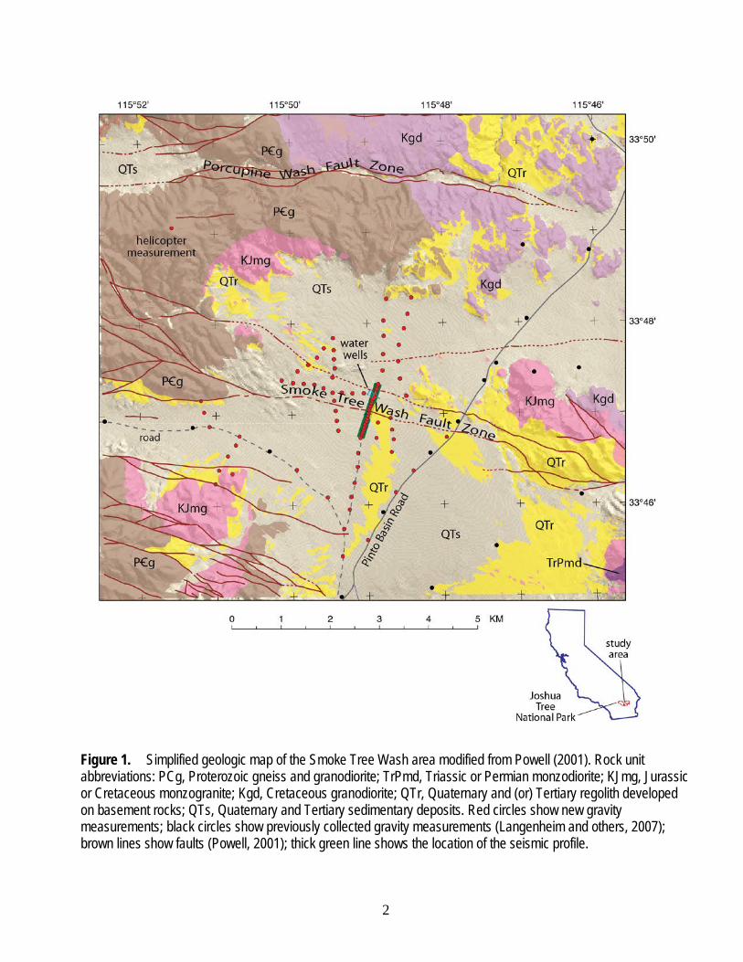
deposits and to delineate geologic structures that might influence groundwater flow beneath the Smoke Tree Wash area (fig. 1). The study area for these geophysical surveys is within Joshua Tree National Park (fig. 1), west of Pinto Basin Road and about 4 km north of the Cottonwood Visitor Center. In this study, we focus on estimating the thickness of the valley-fill deposits in the area of the water well that supplies the visitor center. The well is within the Smoke Tree Wash fault zone, which has 1–1.5 km of left-lateral offset (Hope, 1966; Powell, 1993).

2

Figure 1. Simplified geologic map of the Smoke Tree Wash area modified from Powell (2001). Rock unit abbreviations: PCg, Proterozoic gneiss and granodiorite; TrPmd, Triassic or Permian monzodiorite; KJmg, Jurassic or Cretaceous monzogranite; Kgd, Cretaceous granodiorite; QTr, Quaternary and (or) Tertiary regolith developed on basement rocks; QTs, Quaternary and Tertiary sedimentary deposits. Red circles show new gravity measurements; black circles show previously collected gravity measurements (Langenheim and others, 2007); brown lines show faults (Powell, 2001); thick green line shows the location of the seismic profile.

3

Primary data sets used to determine the thickness of valley-fill deposits include gravity measurements, geologic map information, and driller’s logs of water wells. A seismic-refraction profile (thick green line in fig. 1) along the road that bisects the study area provides independent information on the thickness of, and structure in, the valley-fill deposits. Aeromagnetic data (Langenheim and Hill, 2010) were useful for delineating the main fault strand of the Porcupine Wash fault and its cumulative offset (see Langenheim and Powell, 2009), but not particularly useful for determining the thickness of basin fill or detailed enough to clearly delineate the displacement on individual strands of the Smoke Tree Wash fault. The valley-fill deposits (QTs in fig. 1) consist of locally derived Quaternary and Tertiary sedimentary rocks and sediments (Powell, 2001) and rest on crystalline basement complex rocks that consist of Proterozoic gneiss and granodiorite (PCg on fig. 1) and Mesozoic granitic rocks (fig. 1, units KJmg, TrPmc, and Kgd). We also include various regolith units mapped by Powell (2001; unit QTr in fig. 1) as part of the valley-fill deposits, although the rock density of these units may be higher than the QTs valley fill. The large density contrast between the valley-fill deposits and the crystalline basement complex (here assumed to average 600 kg/m3 in the upper 656 ft [200 m]) makes gravity a useful method for determining the thickness of the valley-fill deposits. Seismic methods are sensitive to velocity contrasts between the high-velocity basement rocks and overlying lower-velocity fill, but seismic velocities can also be affected by fracturing, which reduces velocities more than it does densities (Stierman and Kovach, 1979).

Data Sets Gravity Survey and Reduction

Eighty-nine new gravity measurements (iso_all.txt) were collected in 2008–9 along, and in the vicinity of, the seismic profile, including one measurement by helicopter on Precambrian gneiss and granodiorite in the northwestern part of the study area. A LaCoste Romberg gravity meter (G17C) was used and measurements were tied to base station PB0813 (Roberts and Jachens, 1986); these measurements supplemented data previously collected at 19 sites (Langenheim and others, 2007). Gravity data were reduced using the Geodetic Reference System of 1967 (International Union of Geodesy and Geophysics, 1971) and referenced to the International Gravity Standardization Net 1971 gravity datum (Morelli, 1974, p. 18). Gravity data were reduced to isostatic anomalies using a reduction density of 2,670 kg/m3 and include earth-tide, instrument drift, free-air, Bouguer, latitude, curvature, and terrain corrections. An isostatic correction, using a sea-level crustal thickness of 25 km (16 mi) and a mantle-crust density contrast of 400 kg/m3, was applied to the gravity data to remove the long-wavelength gravitational effect of isostatic compensation of the crust due to topographic loading. The data were gridded at a spacing of 250 m (820 ft), roughly the spacing of gravity stations along the detailed profiles, using a minimum curvature algorithm. The resulting gravity field, termed the isostatic residual gravity anomaly, is shown in figure 2.

Terrain corrections were calculated to a radial distance of 104 mi (167 km) and involved a 3-part process: (1) Hayford-Bowie zones A and B with an outer radius of 223 ft (68 m) were estimated in the field with the aid of tables and charts, (2) Hayford-Bowie zones C and D with an outer radius of 1,936 ft (590 m) were calculated using a 100-ft (30-m) digital elevation model, and (3) terrain corrections from a distance of 1,936 ft (0.59 km) to 104 mi (167 km) were calculated using a digital elevation model and a procedure proposed by Plouff (1977). Total terrain corrections for the stations collected for this study ranged from 0 to 7.87 milliGals (mGal), averaging 1.8 mGal. If the error resulting from the terrain correction is considered to be 5 to 10 percent of the total terrain correction, the largest error from the terrain correction expected for the data is 0.79 mGal, However, the average error (less than 0.2 mGal)

4

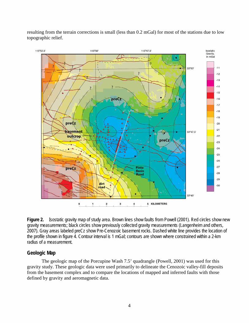
resulting from the terrain corrections is small (less than 0.2 mGal) for most of the stations due to low topographic relief.

Figure 2. Isostatic gravity map of study area. Brown lines show faults from Powell (2001). Red circles show new gravity measurements; black circles show previously collected gravity measurements (Langenheim and others, 2007). Gray areas labeled preCz show Pre-Cenozoic basement rocks. Dashed white line provides the location of the profile shown in figure 4. Contour interval is 1 mGal; contours are shown where constrained within a 2-km radius of a measurement.

Geologic Map The geologic map of the Porcupine Wash 7.5’ quadrangle (Powell, 2001) was used for this

gravity study. These geologic data were used primarily to delineate the Cenozoic valley-fill deposits from the basement complex and to compare the locations of mapped and inferred faults with those defined by gravity and aeromagnetic data.

5

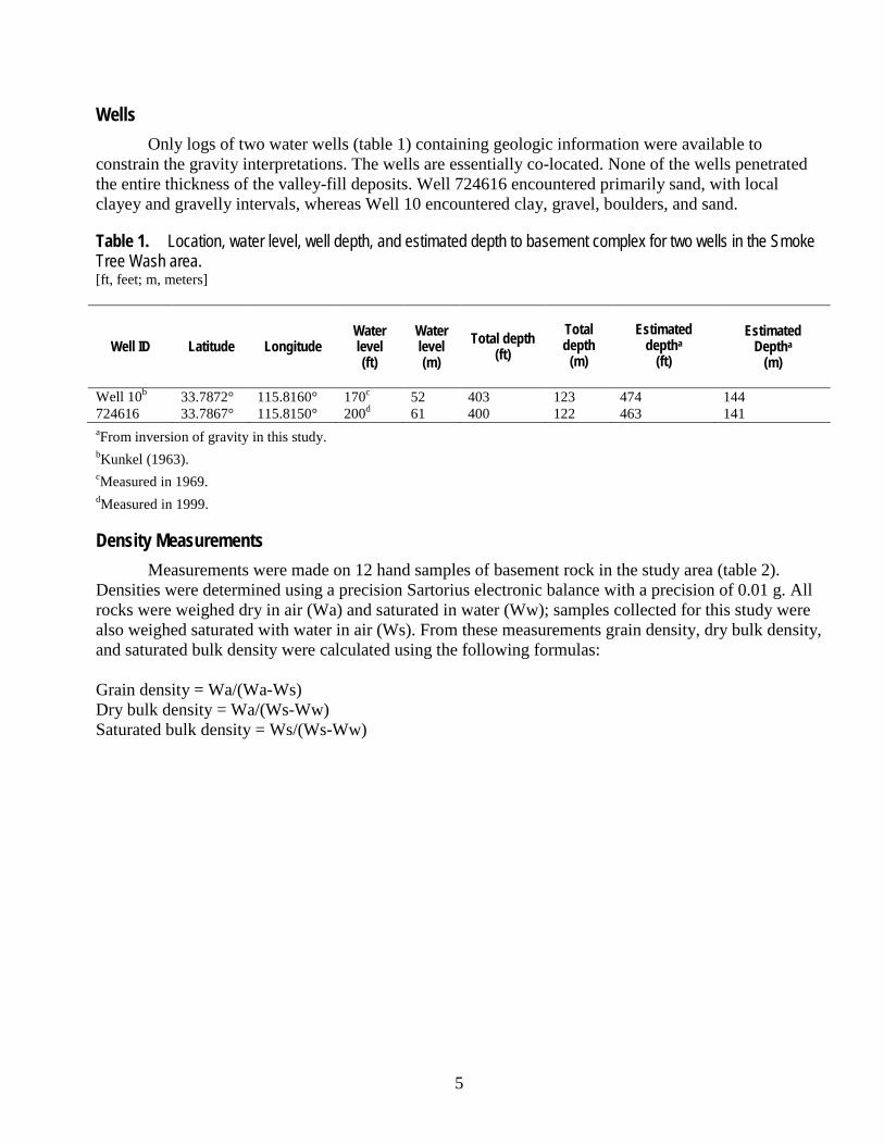
Wells Only logs of two water wells (table 1) containing geologic information were available to

constrain the gravity interpretations. The wells are essentially co-located. None of the wells penetrated the entire thickness of the valley-fill deposits. Well 724616 encountered primarily sand, with local clayey and gravelly intervals, whereas Well 10 encountered clay, gravel, boulders, and sand.

Table 1. Location, water level, well depth, and estimated depth to basement complex for two wells in the Smoke Tree Wash area. [ft, feet; m, meters]

Well ID Latitude Longitude Water level (ft)

Water level (m)

Total depth (ft)

Total depth

(m)

Estimated

deptha (ft)

Estimated Deptha

(m)

Well 10b 33.7872° 115.8160° 170c 52 403 123 474 144 724616 33.7867° 115.8150° 200d 61 400 122 463 141 aFrom inversion of gravity in this study. bKunkel (1963). cMeasured in 1969. dMeasured in 1999.

Density Measurements Measurements were made on 12 hand samples of basement rock in the study area (table 2).

Densities were determined using a precision Sartorius electronic balance with a precision of 0.01 g. All rocks were weighed dry in air (Wa) and saturated in water (Ww); samples collected for this study were also weighed saturated with water in air (Ws). From these measurements grain density, dry bulk density, and saturated bulk density were calculated using the following formulas:

Grain density = Wa/(Wa-Ws) Dry bulk density = Wa/(Ws-Ww) Saturated bulk density = Ws/(Ws-Ww)

6

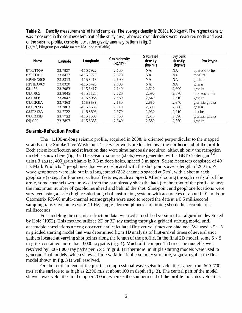
Table 2. Density measurements of hand samples. The average density is 2680±100 kg/m3. The highest density was measured in the southwestern part of the study area, whereas lower densities were measured north and east of the seismic profile, consistent with the gravity anomaly pattern in fig. 2. [kg/m3, kilogram per cubic meter; NA, not available]

Name Latitude

Longitude Grain density (kg/ m3)

Saturated density (kg/ m3)

Dry bulk density (kg/m3)

Rock type

87RJT009 33.7857 -115.7922 2,630 NA NA quartz diorite 87RJT011 33.8477 -115.7777 2,670 NA NA tonalite RPHEX008 33.8313 -115.8418 2,690 NA NA gneiss RPHEX009 33.8320 -115.8423 2,690 NA NA gneiss 03-456 33.7983 -115.8417 2,640 2,610 2,600 granite 08JT005 33.8045 -115.8123 2,620 2,590 2,570 monzogranite 08JT006 33.8047 -115.8068 2,580 2,540 2,510 granite 08JT209A 33.7863 -115.8538 2,650 2,650 2,640 granitic gneiss 08JT209B 33.7863 -115.8538 2,710 2,690 2,680 gneiss 08JT213A 33.7722 -115.8503 2,970 2,930 2,910 diorite 08JT213B 33.7722 -115.8503 2,650 2,610 2,590 granitic gneiss 09jt009 33.7897 -115.8355 2,640 2,580 2,550 granite

Seismic-Refraction Profile The ~1,100-m-long seismic profile, acquired in 2008, is oriented perpendicular to the mapped

strands of the Smoke Tree Wash fault. The water wells are located near the northern end of the profile. Both seismic-reflection and refraction data were simultaneously acquired, although only the refraction model is shown here (fig. 3). The seismic sources (shots) were generated with a BETSY-SeisgunTM using 8 gauge, 400 grain blanks in 0.3 m deep holes, spaced 5 m apart. Seismic sensors consisted of 40 Hz Mark ProductsTM geophones that were co-located with the shot points over a length of 200 m. P-wave geophones were laid out in a long spread (232 channels spaced at 5 m), with a shot at each geophone (except for four near cultural features, such as pipes). After shooting through nearly all of the array, some channels were moved from the part already shot (the back) to the front of the profile to keep the maximum number of geophones ahead and behind the shot. Shot-point and geophone locations were surveyed using a Leica high-resolution global positioning system, with accuracies of about 0.01 m. Four Geometrix RX-60 multi-channel seismographs were used to record the data at a 0.5 millisecond sampling rate. Geophones were 40-Hz, single-element phones and timing should be accurate to 2 milliseconds.

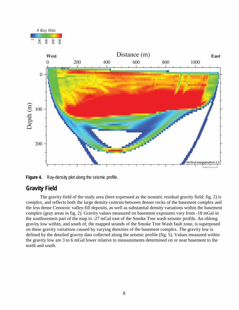
For modeling the seismic refraction data, we used a modified version of an algorithm developed by Hole (1992). This method utilizes 2D or 3D ray tracing through a gridded starting model until acceptable correlations among observed and calculated first-arrival times are obtained. We used a 5 × 5 m gridded starting model that was determined from 1D analysis of first-arrival times of several shot gathers located at varying shot points along the length of the profile. In the final 2D model, some 5 × 5 m grids contained more than 3,000 raypaths (fig. 4). Much of the upper 150 m of the model is well resolved by 500-1,000 ray paths per 5 × 5 m grid. Furthermore, multiple starting models were used to generate final models, which showed little variation in the velocity structure, suggesting that the final model shown in fig. 3 is well resolved.

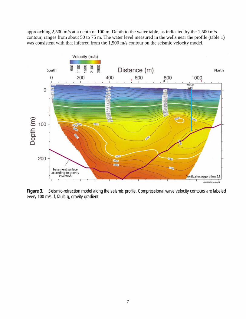
On the northern end of the profile, compressional wave seismic velocities range from 600–700 m/s at the surface to as high as 2,300 m/s at about 100 m depth (fig. 3). The central part of the model shows lower velocities in the upper 200 m, whereas the southern end of the profile indicates velocities

7

approaching 2,500 m/s at a depth of 100 m. Depth to the water table, as indicated by the 1,500 m/s contour, ranges from about 50 to 75 m. The water level measured in the wells near the profile (table 1) was consistent with that inferred from the 1,500 m/s contour on the seismic velocity model.

Figure 3. Seismic-refraction model along the seismic profile. Compressional wave velocity contours are labeled every 100 m/s. f, fault; g, gravity gradient.

8

Figure 4. Ray-density plot along the seismic profile.

Gravity Field The gravity field of the study area (here expressed as the isostatic residual gravity field; fig. 2) is

complex, and reflects both the large density contrast between denser rocks of the basement complex and the less dense Cenozoic valley-fill deposits, as well as substantial density variations within the basement complex (gray areas in fig. 2). Gravity values measured on basement exposures vary from -18 mGal in the southwestern part of the map to -27 mGal east of the Smoke Tree wash seismic profile. An oblong gravity low within, and south of, the mapped strands of the Smoke Tree Wash fault zone, is superposed on these gravity variations caused by varying densities of the basement complex. The gravity low is defined by the detailed gravity data collected along the seismic profile (fig. 5). Values measured within the gravity low are 3 to 6 mGal lower relative to measurements determined on or near basement to the north and south.

9

Figure 5. Gravity data along the seismic line (horizontal red line), extended to the north and south. Vertical magenta lines show the locations of maximum horizontal gravity gradient that coincide with basement outcrops (b), the Smoke Tree Wash fault zone (f), and an inferred strand of that fault zone (i). Locations of strands of mapped faults (Powell, 2001) are indicated.

The gravity field was analyzed to examine the structural setting of the water well in Smoke Tree Wash. The automated method of Blakely and Simpson (1986) was used to determine where changes in rock density are located over a short distance, such as density contrasts caused by fault offsets. Places where the gravity field changes laterally the most (maximum horizontal gradient) mark steeply dipping contacts between rocks of differing densities (density boundaries), such as steep contacts between the dense basement complex and lighter valley-fill deposits. The most pronounced density boundaries (magenta vertical lines in fig. 5) coincide with the Smoke Tree Wash fault zone (f in fig. 5), an inferred

10

strand of that fault zone about 1 km to the south (i in fig. 5), and the basement outcrops (b in fig. 5) at the southwestern part of the map.

Computation Method for Modeling the Thickness of the Valley-Fill Deposits The thickness of the valley-fill deposits (or depth to the basement complex) throughout the study

area was estimated by the method of Jachens and Moring (1990), modified slightly to permit inclusion of constraints at points where the thickness (or minimum thickness) of the valley-fill deposits is known from direct observations in drill holes. An initial estimate of the valley-fill deposits gravity anomaly is made by passing a smooth surface through the gravity values at stations measured where the basement complex rocks crop out (initial estimate of the basement gravity field) and subtracting this surface from the isostatic residual gravity field (fig. 2). This represents only the initial estimate because the gravity values at points on basement complex that lie close to the valley-fill deposits are sensitive to the low-density valley-fill deposits, and are therefore lower than they would be if the valley-fill deposits were not present. To compensate for this effect, the initial valley-fill deposits gravity anomaly is used to calculate an initial estimate of the thickness of the valley-fill deposits, and the gravity effect of these valley-fill deposits is calculated at all of the basement gravity stations. A second estimate of the basement gravity field is then made by passing a smooth surface through the basement gravity values corrected by the valley-fill effect and the process is repeated to produce a second estimate of the thickness of the valley-fill deposits. This process is repeated until further steps do not result in significant changes to the modeled thickness of the valley-fill deposits, usually in five or six steps.

The valley-fill deposits gravity anomaly was converted to thickness of the valley-fill deposits using an assumed density contrast that varies with depth (table 3) between the sedimentary deposits that make up the valley-fill deposits and the underlying basement complex. This density-depth relation was derived for the Eastern Transverse Ranges (Langenheim and Powell, 2009) based on seismic-velocity measurements about 10 km south of our study area (Blackman, 1988); there are no available sonic logs near the study area. The resulting density contrast of 600 kg/m3 for the upper 660 ft (200 m) of valley-fill deposits is reasonable for Quaternary continental deposits overlying Mesozoic and older crystalline rocks and is also consistent with the velocities measured in the upper 200–250 m along the Smoke Tree seismic refraction profile using the relation of Gardner and others (1974). Using the relation in table 1 of Brocher (2005), the density contrasts would be higher, leading to thinner basin fill. The reasonableness of this selected density contrast, at least for the broader Joshua Tree National Park area, was further tested by examining the basement gravity field for any indications of local anomalies at the sites where wells penetrated the basement complex, and the solution was constrained to honor those data. Note that a 10 percent decrease in the density contrast produces an average 20 percent increase in basin thickness for the study area.

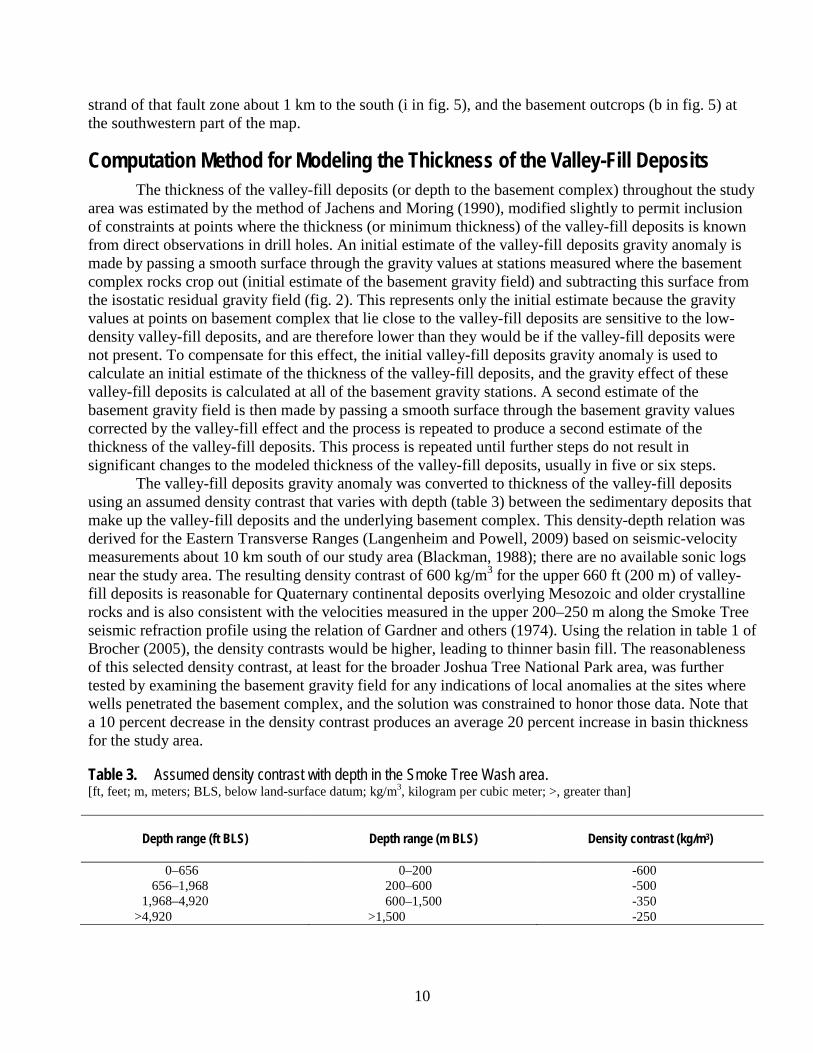
Table 3. Assumed density contrast with depth in the Smoke Tree Wash area. [ft, feet; m, meters; BLS, below land-surface datum; kg/m3, kilogram per cubic meter; >, greater than]

Depth range (ft BLS) Depth range (m BLS) Density contrast (kg/m3)

0–656 0–200 -600 656–1,968 200–600 -500

1,968–4,920 600–1,500 -350 >4,920 >1,500 -250

11

Gravity Results Results of the gravity inversion are shown in figure 6 as a map of thickness of the valley-fill

deposits or subsurface depth to basement rocks. Uncertainties in the gravity data mean that the best resolution that can be expected, even in areas of good gravity coverage, is about ±15 m (50 ft), and resolution is likely less in areas of poor gravity coverage or in areas far from basement outcrop. Also, because the calculations were performed on grid cells 250 m (820 ft) on a side, the results represent averages of the thickness of the valley-fill deposits over this cell size. Thus, variations of the thickness of the valley-fill deposits over distances less than the cell-dimension are not resolved. Finally, gravity data reflect the average shape of the causative body (in this case the thickness of the valley-fill deposits) and the averaging becomes more pronounced the farther from the source that the observations are taken. As a result, places where the valley-fill deposits are the thickest will be subject to higher degrees of averaging, and thus will appear smoother than areas where the valley-fill deposits are thinner. Uncertainty also arises from incomplete knowledge of the gravity field that results from density variations in the basement rocks. The gravity map and profile (figs. 2 and 5) clearly show gravity values in the southern part of the map area that are 4–6 mGal higher than those measured on basement outcrops to the north and east, thus indicating that basement density variations are present in the study area. These variations are taken into account by the inversion, but the field is incompletely known particularly south of the Smoke Tree Wash fault zone where there are no nearby basement outcrops.

12

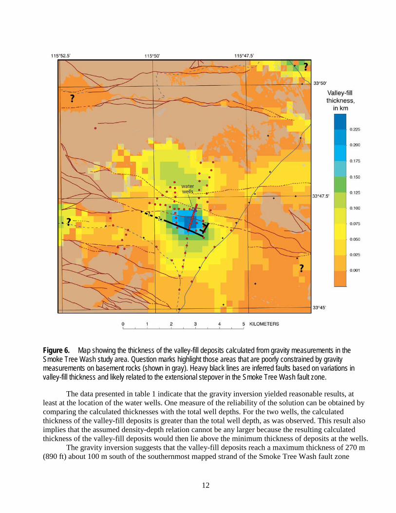
Figure 6. Map showing the thickness of the valley-fill deposits calculated from gravity measurements in the Smoke Tree Wash study area. Question marks highlight those areas that are poorly constrained by gravity measurements on basement rocks (shown in gray). Heavy black lines are inferred faults based on variations in valley-fill thickness and likely related to the extensional stepover in the Smoke Tree Wash fault zone.

The data presented in table 1 indicate that the gravity inversion yielded reasonable results, at least at the location of the water wells. One measure of the reliability of the solution can be obtained by comparing the calculated thicknesses with the total well depths. For the two wells, the calculated thickness of the valley-fill deposits is greater than the total well depth, as was observed. This result also implies that the assumed density-depth relation cannot be any larger because the resulting calculated thickness of the valley-fill deposits would then lie above the minimum thickness of deposits at the wells.

The gravity inversion suggests that the valley-fill deposits reach a maximum thickness of 270 m (890 ft) about 100 m south of the southernmost mapped strand of the Smoke Tree Wash fault zone

13

(Powell, 2001). As defined by thicknesses greater than 100 m, the basin is about 2–2.5 km long and almost 1 km wide. Its morphology (twice as long as wide) and elongation along the strike of the Smoke Tree Wash fault zone suggests a pull-apart basin or extensional stepover (Aydin and Nur, 1982). Gravity gradients along the detailed profile (fig. 4) suggest additional faults that may be projections of mapped faults from the west and east.

Comparison with the Seismic-Refraction Model The basin floor, modeled from the gravity, is deepest in the middle of the seismic line (at a

model distance of 500 m; fig. 3). The basin shallows more steeply to the north than to the south. Velocity contours also deepen in the center of the seismic model below depths of about 100 m (fig. 3). A mapped strand of the Smoke Tree Wash fault bisects this low-velocity area. A steep gravity gradient coincides with the northern margin of the low-velocity area, and may reflect a fault strand that bounds the basin. About 50 m north of the water well, another fault strand coincides with slightly lower velocities at depths of about 100 m. Lower velocities within a fault zone, which result from decreases in the bulk and shear moduli caused by shearing and fracturing of the rock, are consistent with numerous empirical and laboratory studies (Stierman and Kovach, 1979; Moos and Zoback, 1983; Brocher, 2005). However, because gravity values are largely unchanging across this part of the profile, there are not significant changes in density within the fault zone.

There is no obvious relation between the basement surface inferred from the gravity inversion and the velocity of the rocks corresponding to the gravity-inferred basement depth. If the gravity-derived basin model is accurate, the velocity model suggests that there are density variations within the valley-fill deposits. Using the relation of Gardner and others (1974) the variation in valley-fill density, inferred from the velocity model, may be as much as 120 kg/m3. Such a density contrast implies a porosity change of 5 percent.

Uncertainty in the density and velocity of the basement rocks leads to multiple plausible interpretations of the gravity and seismic models. The highest velocity within the velocity model is about 2,600 m/s, which is inconsistent with the velocity of unweathered and unfractured granite (Brocher, 2008) and more typical of sedimentary rocks. In other seismic-refraction studies in southern California, velocities of 4 km/s or higher in the near surface have been interpreted as basement rocks (Catchings and others, 2000, 2002, 2008, 2009). Thus, one interpretation is that the seismic profile did not image the basement surface and that the gravity-defined basement surface is actually too shallow, implying that the density contrasts used in the inversion (table 3) are too large. Alternatively, the basement rocks may be sheared along the Smoke Tree Wash fault zone and may be characterized by significantly lower velocities than typical for basement rocks; velocity and density measurements from a well 600 m deep within quartz diorite about 1 km away from the San Andreas Fault (Stierman and Kovach, 1979) indicate velocities of 2,000–3,500 m/s and densities of 2,390–2,620 kg/m3, compared to 4,500–6,500 m/s and 2,660–2,740 kg/m3, respectively, in unfractured quartz diorite.

Regardless of the uncertainty in the basement surface, the models indicate a low-density, low-velocity region that is bisected by at least one strand of the Smoke Tree Wash fault. One interpretation is that this Smoke Tree Wash fault strand is the youngest strand. The basin shape inverted from the gravity data implies a pull-apart basin; sandbox models (Dooley and McClay, 1997) indicate that faulting in pull-apart basins evolves such that younger fault strands commonly bisect the basin. Another interpretation is that the low-velocity region in the middle of the model represents a thick weathered regolith—both residual and slightly transported—that was a widespread feature regionally developed on granitic rocks that were exposed in the Tertiary (see Powell and Matti, 2000; Powell and others, 2015). In this scenario the irregular pattern of velocity distribution in the 2,200–2,300 m/s range might reflect

14

lateral variability produced during the regolith weathering process. These two interpretations are not mutually exclusive. A longer seismic profile that extends onto basement outcrops and samples deeper beneath the fault zone would help to refine the interpretation of the geophysical data.

Acknowledgments The National Park Service and the National Cooperative Geologic Mapping and Earthquake

Hazards programs of the U.S. Geological Survey provided funding for this study. We gratefully acknowledge Luke Sabala, physical scientist for Joshua Tree National Park, for logistical assistance and support. Tom Brocher and Bob Jachens provided helpful reviews, which substantially improved the report.

References Aydin, Attila, and Nur, Amos, 1982, Evolution of pull-apart basins and their scale independence:

Tectonics, v. 1, p. 91–105. Blackman, T.D., 1988, Geophysical investigations of the Hayfield Dry Lake area in the western

Chuckwalla valley, southern California: Riverside, University of California, M.S. thesis, 101 p. Blakely, R.J., and Simpson, R.W., 1986, Approximating edges of source bodies from magnetic or

gravity anomalies: Geophysics, v. 51, p. 1,494–1,498. Brocher, T.M., 2005, Empirical relations between elastic wavespeeds and density in the Earth’s crust:

Bulletin of Seismological Society of America, v. 95, p. 2,081–2,092. Brocher, T.M., 2008, Compressional and shear-wave velocity versus depth relations for common rock

types in northern California: Bulletin of the Seismological Society of America, v. 98, p. 950–968. Catchings, R.D., Cox, B.F., Goldman, M.R., Gandhok, G., Rymer, R.J., Dingler, J., and Martin, P.,

2000, Subsurface structure and seismic velocities as determined from high-resolution seismic imaging in the Victorville, California area—Implications for water resources and earthquake hazards: U.S. Geological Survey Open-File Report 00-123, 70 p.

Catchings, R.D., Rymer, M.J., Goldman, M.R., and Gandhok, G., 2009, San Andreas fault geometry at Desert Hot Springs, California, and its effects on earthquake hazards and groundwater: Bulletin of the Seismological Society of America, v. 99, p. 2,190–2,207.

Catchings, R.D., Rymer, M.J., Goldman, M.R., Gandhok, G., and Steedman, C.E., 2008, Structure of the San Bernardino basin along two seismic transects: Rialto-Colton to the San Andreas fault and along the I-215 Freeway (I-10 to SR30): U.S. Geological Survey Open-File Report 2008-1197, 70 p.

Catchings, R.D., Rymer, M.J., Goldman, M.R., Hole, J.A., Huggins, R., and Lippus, C., 2002, High-resolution seismic velocities and shallow structure of the San Andreas fault at Middle Mountain, Parkfield, California: Bulletin of the Seismological Society of America, v. 92, p. 2,493–2,503.

Dooley, Tim, and McClay, Ken, 1997, Analog modeling of pull-apart basins: American Association of Petroleum Geologists Bulletin, v. 81, p. 1,804–1,826.

Gardner, G.H.F., Gardner, L.W., and Gregory, A.R., 1974, Formation velocity and density—The diagnostic basis for stratigraphic traps: Geophysics, v. 39, p. 770–780.

Hole, J.A., 1992, Nonlinear high-resolution three-dimensional travel time tomography: Journal of Geophysical Research, v. 97, p. 6,553–6,562.

Hope, R.A., 1966, Geology and structural setting of the eastern Transverse Ranges, southern California: Los Angeles, University of California, Ph.D. dissertation, 201 p.

International Union of Geodesy and Geophysics, 1971, Geodetic reference system 1967: International Association of Geodesy Special Publication no. 3, 116 p.

15

Jachens, R.C., and Moring, B.C., 1990, Maps of the thickness of Cenozoic deposits and the isostatic residual gravity over basement for Nevada: U.S. Geological Survey Open-File Report 90–404, 15 p., 2 plates.

Kunkel, Fred, 1963, Hydrologic and geologic reconnaissance of Pinto Basin, Joshua Tree National Monument, Riverside County, California: U.S. Geological Survey Water Supply Paper 1475-O, p. 537–561.

Langenheim, V.E., Biehler, Shawn, McPhee, D.K., McCabe, C.M., Watt, J.T., Anderson, M., Chuchel, B.A., and Stoffer, P., 2007, Preliminary isostatic gravity map of Joshua Tree National Park and vicinity, southern California: U.S. Geological Survey Open-File Report 2007–1218, scale 1:100,000.

Langenheim, V.E., and Hill, P.L, 2010, Preliminary aeromagnetic map of Joshua Tree National Park and vicinity, southern California: U.S. Geological Survey Open-File Report 2010-1070, scale 1:100,000.

Langenheim, V.E., and Powell, R.E., 2009, Basin geometry and cumulative offsets in the Eastern Transverse Ranges, southern California—Implications for transrotational deformation along the San Andreas fault system: Geosphere, v. 5, no, 1, p. 1–22; doi:10.1130/GES00177.

Moos, Daniel, and Zoback, M.D., 1983, In situ studies of velocity in fractured crystalline rocks: Journal of Geophysical Research, v. 88, p. 2,345–2,358.

Morelli, Carlo, 1974, The international gravity standardization net, 1971: International Association of Geodesy Special Publication no. 4, 194 p.

Plouff, Donald, 1977, Preliminary documentation for a FORTRAN program to compute gravity terrain corrections based on topography digitized on a geographic grid: U.S. Geological Survey Open-File Report 77–535, 45 p.

Powell, R.E., 1993, San Andreas Fault, in Powell, R.E., Weldon, R.E., II, and Matti, J.C., eds., The San Andreas Fault System—Displacement, palinspastic reconstruction, and geologic evolution: Geological Society of America Memoir 178, p. 1–106.

Powell, R.E., 2001, Geologic map and digital database of the Porcupine Wash 7.5 minute quadrangle, Riverside county, California: U.S. Geological Survey Open-File Report 01–030, accessed November 15, 2005, at http://pubs.usgs.gov/of/2001/0030/

Powell, R.E., and Matti, J.C., 2000, Geologic map and digital database of the Cougar Buttes 7.5' Quadrangle, San Bernardino County, California: U.S. Geological Survey Open-File Report 00–175, accessed January 15, 2012, at http://pubs.usgs.gov/of/2000/0175/.

Powell, R.E., Matti, J.C., and Cossette, P.M., 2015, Geology of Joshua Tree National Park geodatabase: U.S. Geological Survey Open-File Report 2015–1175, accessed September 30, 2015, at http://dx.doi.org/10.3133/ofr20151175.

Roberts, C.W., and Jachens, R.C., 1986, High-precision gravity stations for monitoring vertical crustal motion in southern California: U.S. Geological Survey Open-File Report 86-44, 76 p.

Stierman, D.J., and Kovach, R.L., 1979, An in situ velocity study—The Stone Canyon well: Journal of Geophysical Research, v. 84, p. 672–678.