Secular Stagnation: Theory and Remedies

Jean-Baptiste MICHAU

September 2015

Cahier n° 2015-13

ECOLE POLYTECHNIQUE CENTRE NATIONAL DE LA RECHERCHE SCIENTIFIQUE

DEPARTEMENT D'ECONOMIE Route de Saclay

91128 PALAISEAU CEDEX

(33) 1 69333033

http://www.economie.polytechnique.edu/ mariame.seydi@polytechnique.edu

Secular Stagnation: Theory and Remedies

Jean-Baptiste Michau�

Ecole Polytechnique

September 2015

Abstract

This paper relies on a Ramsey model with money to o¤er a simple theory of

secular stagnation. The permanent failure of the economy to produce at full ca-

pacity results from three features: (i) The combination of the zero lower bound on

the nominal interest rate and of an in�ation ceiling imposes a lower bound on the

real interest rate; (ii) Some dynastic households have a high propensity to save, due

to a preference for wealth; (iii) A downward wage rigidity breaks the de�ationary

spiral resulting from the lack of demand. In this framework, I derive the paradox

of �exibility, of thrift, and of toil.

If the in�ation ceiling cannot be raised, then the government needs to rely on

�scal policy to escape secular stagnation. However, a conventional �scal stimulus

is not an e¢ cient response to a permanent liquidity trap, and can even be welfare

reducing. The solution is instead to tax household wealth and to subsidize income

from physical capital, through an investment subsidy or a reduction in the taxation

of corporate income. This optimal policy is revenue neutral and implements the

�rst-best allocation of resources. However, to avoid a jump in the price level upon

implementation of the optimal policy, the government needs to redeem the money

that had previously been supplied to �nance public de�cits.

Keywords: Liquidity trap, Monetary and �scal policy, Secular stagnation

JEL Classi�cation: E12, E31, E62, E63

1 Introduction

Keynes (1936) explained how an economy can be depressed due to a lack of demand.

Indeed, if households�demand for consumption and �rms�demand for investment are

excessively low, then the economy fails to produce at full capacity. While the resulting

�Contact: Jean-Baptiste.Michau@polytechnique.edu

1

depressions are usually seen as an extreme manifestation of a business cycle phenomenon,

Hansen (1939) was the �rst to worry that it might be a permanent state of a¤airs. This

is the "secular stagnation" hypothesis.

When aggregate demand is weak, in�ation declines and the central bank responds by

aggressively cutting the nominal interest rate such as to stimulate demand. However,

a fundamental constraint on monetary policy is that the nominal interest rate cannot

be negative. Indeed, no-one is willing to pay more than $100 for a bond yielding $100

in the future. In the mid-1990s, Japan was the �rst large industrialized country to hit

the zero lower bound and to fall into the liquidity trap. Its subsequent history, with

an economy mired in very low in�ation and weak GDP growth, suggests that there is

no mechanism through which an economy naturally recovers from a persistent lack of

demand. Moreover, Japan is facing a policy conundrum as aggregate demand remains

desperately weak despite a budget de�cit of about 7% of GDP, a debt-to-GDP ratio of

230%, and substantial monetary accommodation.

Over the past few years, there has been growing concerns that the U.S. and the Eu-

rozone might be in a similar situation as Japan. In particular, Summers (2014) has

emphasized that the credit boom of 2003-2007 in the U.S. did not generate a correspond-

ing economic boom, which suggests that the unsustainable demand for consumption of

poor borrowers was hiding an already weak level of demand of rich lenders.

Despite the prominence of the secular stagnation hypothesis in the policy debate,

there has been few attempts to model it explicitly. In this paper, I o¤er a simple theory

of secular stagnation, on which I then rely for a careful policy analysis. The structure

of the model is a Ramsey economy with money and �exible prices, to which I add three

features.

First, I assume that the central bank imposes a ceiling on in�ation. This, together

with the zero lower bound on the nominal interest rate, generates a lower bound on the

real interest rate. In most industrialized countries, central banks never allow in�ation to

exceed 2%, which prevents the real interest rate from ever falling below -2%.

Second, I assume that households derive utility from holding wealth. This can raise

their propensity to save to such an extent that a negative real interest rate is necessary

for the economy to produce at full capacity. Importantly, in�nitely lived households

should be interpreted as dynasties. Hence, bequest motives are important determinants

of the saving behavior of households. In particular, we know that pure altruism alone

cannot account for the observed patterns of bequests (Kopczuk 2009). Instead, parents

seem to be commonly motivated by the "joy of giving". A "capitalist spirit" also induces

many individuals to derive intrinsic utility from the accumulation of wealth, which is then

passed on from generation to generation (Carroll 2000, Kopczuk 2007).1 While I rely for

1Also, Piketty (2011) relies on a model with wealth in the utility to show that the inheritance-to-

2

simplicity on a representative household model, my results only require that a strictly

positive mass of households has a preference for wealth. Indeed, a well known result in

macroeconomics is that the real interest must eventually be determined by the behavior

of the most patient households. This is highly relevant as the rise in inequality is often

cited as a major cause of the recent decline in aggregate demand (Summers 2014). A

preference for wealth seems a natural explanation for the concentration of wealth in the

hands of a small number of households with a very low propensity to spend (Kumhof,

Rancière and Winant 2015).

Finally, I impose a downward wage rigidity. If the in�ation ceiling is su¢ ciently

low and the preference for wealth su¢ ciently strong, then aggregate demand is smaller

than aggregate supply. This reduces in�ation, which raises the real interest rate, which

further contracts aggregate demand. To have a stationary secular stagnation equilibrium,

I therefore need to put a break on the de�ationary spiral. This is achieved through the

downward wage rigidity.

In the secular stagnation equilibrium, aggregate demand is depressed. This induces

�rms�labor demand to fall short of workers�labor supply. However, this ine¢ ciency is

primarily due to the lower bound on the real interest rate, not to the downward wage

rigidity. Indeed, if wages are more �exible, then in�ation is smaller, the real interest

is higher, and the economy is even more depressed. Conversely, for a su¢ ciently high

in�ation ceiling, there always exists a frictionless steady state equilibrium where the

economy produces at full capacity.2

The obvious policy response to secular stagnation is to raise the in�ation ceiling.

However, in most countries, this seems politically and institutionally out of reach. Hence,

I explore alternative remedies. A simple policy analysis con�rms that the usual set of

tools used for macroeconomic stabilization are not adequate in the context of secular

stagnation. Increasing the money supply through open market operations is useless in a

liquidity trap. A helicopter drop of money that is su¢ ciently large to induce the economy

to produce at full capacity is inconsistent with the in�ation ceiling. A �scal stimulus raises

�rms�demand for labor much more than workers�consumption level. Hence, it is likely

to be welfare reducing, even though the government spending multiplier is typically well

above 1.

However, with a wider set of policy instruments, the government can implement the

�rst-best allocation of resources without raising the in�ation ceiling. To understand

this result, note that secular stagnation is fundamentally due to an excessively high real

income ratio is a rising function of r� g, consistently with the historical experience of France from 1820to 2009.

2Interestingly, in the secular stagnation equilibrium, in�ation is essentially determined by the down-ward wage rigidity. Hence, the real interest rate is typically well above its lower bound, which results ina very depressed level of aggregate demand.

3

interest rate. This creates two distortions. First, it raises the cost of capital. This

reduces the demand for investment, resulting in depressed capital-labor ratio. Second, a

high real interest rate reduces the demand for consumption. The �rst distortion should

be addressed by subsidizing the income from physical capital. This can either be achieved

through an investment subsidy or a reduction in the taxation of corporate income. The

second distortion can be o¤set through a wealth tax, which reduces the e¤ective real

interest rate faced by consumers. This policy is revenue neutral and it exactly replicates

the allocation of resources that would result from an increase in the in�ation ceiling.

By inducing the economy to produce at full capacity, the optimal policy makes the

price level proportional to the money supply. Hence, to prevent a jump in the price level

upon implementation of the policy, the government must redeem the money supply that

is not used for transactions. This suggests that relying on the printing press to �nance

some stimulus can eventually make the government reluctant to implement the optimal

policy.

Related Literature. Secular stagnation is a stationary phenomenon. However, in

typical models of the liquidity trap, the binding zero lower bound forces the real interest

rate to be above households�discount rate (Krugman 1998, Eggertsson and Woodford

2003, Werning 2012). This induces households to adopt a rising path of consumption,

which is inconsistent with stationarity. A model of secular stagnation must therefore

reconcile an excessively high real interest rate, which depresses aggregate demand, with

the existence of a stationary equilibrium.

Eggertsson and Mehrotra (2014) solved the problem by relying on an overlapping

generation model without altruistic links. In their theory of secular stagnation, aggregate

demand is either depressed because of a low rate of population growth or because the

economy has been hit by a deleveraging shock.3 Interestingly, to eliminate the output

gap, the government can either increase its spending or redistribute income from lenders

to borrowers.

Kocherlakota (2013) showed that, with overlapping generations or credit constraints,

secular stagnation can result from a fall in the price of land. Caballero and Farhi (2015)

relied on a perpetual youth model with risky assets to o¤er an alternative theory of secular

stagnation where the lack of demand is due to a shortage of safe assets. To escape the

depression, the government should either allow in�ation to increase or raise the supply

of public debt, possibly by buying private risky assets.

My contribution to this literature is to show that secular stagnation can be derived in

a Ramsey economy where some households have a preference for wealth. Under a dynastic

interpretation of in�nitely lived households, my work shows that altruistic links across

3They also considered the possibility that demand is depressed due to a rise in inequality, whereagents with low propensity to consume become wealthier, or to a fall in the price of investment goods.

4

generations are not inconsistent with the existence of a stationary secular stagnation

equilibrium. On the contrary, the bequest motive seems to be a natural justi�cation for

the preference for wealth that delivers stationarity. The Ramsey framework is convenient

for policy analysis. This allows me to characterize the optimal policy that implements the

�rst-best allocation of resources without raising the in�ation ceiling. Also, by introducing

money into the economy, I can investigate the monetary �nancing of public de�cits.

In a related contribution, Michaillat and Saez (2015) o¤er a model of the business cycle

where self-employed households exchange their labor services under matching frictions.

As prices and market tightness are not independently determined, they focus on an

equilibrium where in�ation is constant and where market tightness adjusts such as to

equate aggregate demand to aggregate supply. Hence, business cycle �uctuations result in

ine¢ cient �uctuations in market tightness. To have a permanent liquidity trap, they also

assume that households have a preference for wealth. Interestingly, as a lack of demand

does not translate into lower in�ation, they do not obtain the Keynesian paradoxes.

Another strand of the literature has emphasized the role of expectations. Benhabib,

Schmitt-Grohé and Uribe (2001) showed that, if the central bank follows a Taylor rule,

then self-ful�lling expectations can induce the economy to fall into a permanent liquidity

trap. Benigno and Fornaro (2015) proposed a theory of "stagnation traps" where the

weakness of aggregate demand depresses investment in innovation, resulting in a low rate

of technological progress. This pushes the nominal interest rate against the zero lower

bound, which explains why aggregate demand remains so weak. In that context, subsidies

to investment in innovation are welfare enhancing.

The optimal policy that I derive is similar to the "unconventional �scal policy" of

Correia, Farhi, Nicolini and Teles (2013). They showed that, in a new Keynesian model,

it is possible to replicate a negative nominal interest rate by implementing a rising path of

consumption taxes, to induce agents to front-load their demand for consumption, together

with a falling path of labor income taxes, to o¤set the resulting distortion to labor

supply. In the presence of capital, this policy must be supplemented with a temporary

capital subsidy. However, they only considered a temporary liquidity trap. By contrast,

under secular stagnation, the economy is permanently liquidity trapped. I therefore

restrict my attention to stationary policies. Eggertsson (2010) also showed that some

�scal instruments can be relied upon to stimulate aggregate demand.

The paper is organized as follows. Section 2 presents the representative household

model of secular stagnation. In Section 3, I discuss some important properties of the

secular stagnation equilibrium. In Section 4, I investigate the e¤ectiveness of conventional

macroeconomic stabilization policies. The optimal policy is derived in Section 5. The

implications of heterogeneity are brie�y discussed in Section 6. The paper ends with a

conclusion.

5

2 The Representative Household Model

2.1 Households

Time is continuous. There is a mass 1 of in�nitely lived households. Each household

consumes a quantity ct of a single consumption good with price Pt. It supplies labor ltpaid at nominal wage Wt and receives a real lump-sum transfer t. The nominal wealth

At of a household is composed of physical capital Kt, government bonds Bt, and money

Mt:

At = PKt Kt +Bt +Mt; (1)

where PKt denotes the nominal price of capital. Firms pay Rt to rent capital from

households. Capital depreciates at rate �. There are three components to the nominal

return from a unit of physical capital: the rent Rt, the loss due to depreciation �PKt , and

the capital gain _PKt . Bonds yield a nominal return it, while money yields a zero nominal

return. The wealth of the representative household therefore evolves according to:

_At =hRt � �PKt +

_PKt

iKt + itBt +Wtlt + Pt t � Ptct;

= itAt +

"RtPKt

� � +_PKtPKt

� it

#PKt Kt � itMt +Wtlt + Pt t � Ptct: (2)

Let �t = _Pt=Pt denote the rate of in�ation, rt = it��t the real interest rate, wt = Wt=Pt

the real wage, at = At=Pt the real household wealth,mt =Mt=Pt the real money holdings,

and pKt = PKt =Pt the real price of capital, measured in units of consumption good.

Dividing the wealth accumulation equation by the price level Pt, while using the fact

that _At=Pt = _at + �tat and _PKt =PKt = _pKt =p

Kt + �t, yields:

_at = rtat +

�RtPKt

� � +_pKtpKt� rt

�pKt Kt � itmt + wtlt + t � ct: (3)

In the absence of uncertainty, by arbitrage, the returns from holding capital must be

equal to the returns from holding bonds. Thus, the second term on the right hand side of

(3) must be equal to zero, which yields the following relationship between the user cost

of capital and the real interest rate:

rt =RtPKt

� � +_pKtpKt

: (4)

The wealth accumulation equation therefore simpli�es to:

_at = rtat � itmt + wtlt + t � ct: (5)

6

The intertemporal budget constraint prevents households from running Ponzi schemes:

limt!1

e�R t0 rsdsat � 0: (6)

The representative household discounts the future at rate � > 0. At any point in time,

it derives utility u (ct) from consuming ct, with u0 (�) > 0, u00 (�) < 0, and limc!0 u0 (c) =

1. It also derives utility h (mt) from holding real money balances mt, with h0 (�) > 0,

h00 (�) < 0, limm!0 h0 (m) = 1, and h0 (m) = 0 for all m � �m. At �m, the household

is satiated with real money balances and does not derive any utility from holding more

money for transaction purposes. The household incurs disutility v (lt) from supplying

labor lt, with v0 (�) > 0, v00 (�) > 0, v0 (0) = 0, and liml!�l v0 (l) = 1 where �l is the

maximum feasible supply of labor, which can be in�nite. The household also derives

utility from holding wealth at. However, it knows that it will eventually need to cover the

liabilities of the government, which are composed of the real aggregate supply of public

debt bst and of money mst . The utility derived by a household from holding wealth is

therefore equal to (at � (bst +mst)), with

0 (�) > 0, 00 (�) � 0, and limK!0 0 (K) <1.

Finally, at any time t, utility is additively separable between its four components. The

intertemporal utility function is therefore given by:Z 1

0

e��t [u (ct)� v (lt) + h (mt) + (at � (bst +mst))] dt: (7)

Including the government liabilities bst + mst into the utility function ensures that

the Ricardian equivalence holds and that the model has reasonable welfare properties.

Indeed, if households did derive utility from holding wealth independently of the level of

government liabilities, then the government would be able to arti�cially increase welfare

by giving households a huge lump-sum subsidy that would eventually be o¤set by a huge

lump-sum tax. This would increase both the level of public debt bst and the wealth atof households and, hence, their welfare. At the zero lower bound, money and bonds are

perfect substitutes and welfare could also be arti�cially increased by raising the aggregate

money supply mst . I therefore assume that the government cannot mechanically raise

welfare by increasing the level of public liabilities. Note that, in the interesting special case

where the marginal utility of wealth is constant, the behavior of households is identical

whether or not government liabilities are included in the utility function.

The household�s problem is to maximize intertemporal utility, (7), subject to the

budget constraint, (5) and (6), with a0 given. Importantly, the paths of public debt bst and

of aggregate money supply mst from time 0 onwards are exogenous to the representative

household�s actions. By the maximum principle, the solution to the household�s problem

7

is characterized by:

_ctct=

�rt � �+

0 (at � (bst +mst))

u0 (ct)

�u0 (ct)

�u00 (ct) ct; (8)

v0 (lt) = wtu0 (ct) ; (9)

h0 (mt) = itu0 (ct) ; (10)

together with the transversality condition:

limt!1

e��tu0 (ct) at = 0: (11)

When it = 0, there is no opportunity cost of holding money rather than bonds. In

that case, the household�s utility from real money balances must be satiated. Moreover,

when it = 0, money and bonds are both zero interest yielding assets that can be used

for saving, i.e. they are perfect substitutes. The household is therefore happy to rely on

money for saving and, hence, its demand for real money balances can be anything greater

or equal to �m. The zero lower bound on the nominal interest rate it therefore follows

from the money demand equation (10).

2.2 Firms

Firms rent capital Kdt from households and employ labor Lt to produce output yt using

a constant returns to scale neoclassical production function:

yt = F�Kdt ; Lt

�: (12)

They choose their demand for capital Kdt and for labor Lt such as to maximize their

pro�ts:

PtF�Kdt ; Lt

��RtK

dt �WtLt: (13)

In equilibrium, each factor of production must be paid its marginal product:

RtPt= FK

�Kdt ; Lt

�; (14)

wt =Wt

Pt= FL

�Kdt ; Lt

�: (15)

By assumption, one unit of output can either be transformed into a consumption good

or an investment good.4 Hence, if investment is strictly positive, then the price of capital

must be equal to that of consumption, i.e. pKt = PKt =Pt = 1. In that case, by (4) and

4However, investment goods cannot be transformed into consumption goods, i.e. investment cannotbe negative.

8

(14), the real interest rate must be given by:

rt = FK�Kdt ; Lt

�� �: (16)

This expression applies in steady state where investment must be strictly positive to

compensate the depreciation of capital.

2.3 Government

Let M st and m

st denote the nominal and real money supply at time t, respectively. The

growth rate of the nominal money supply at t is given by �t = _M st =M

st . We therefore

have M st = M0e

R t0 �sds, where the initial money supply M0 is assumed to be exogenously

given.5 The supply of money by the government is therefore characterized by �t for all

t 2 [0;+1).At any time t, the government gets real revenue _M s

t =Pt from seigniorage, it incurs

real expenditures gt, and it makes a lump-sum transfer t to each household. Thus, the

nominal supply Bst of government bonds evolves according to:

_Bst = itB

st + Pt t + Ptgt � _M s

t : (17)

Thus, using the fact that _Bst =Pt =

_bst + �bst , the real level of public debt bst = Bs

t =Pt

evolves according to:

_bst = (it � �t) bst + t + gt �

_M st

M st

M st

Pt;

= rtbst + t + gt � �tm

st : (18)

Note that �tmst = _M s

t =Pt = _mst + �tm

st . Thus, expression (18) for the accumulation of

public debt can also be written as:

_bst + _mst = rt [b

st +ms

t ] + t + gt � itmst : (19)

Integrating the debt accumulation equation (18) gives:

e�R t0 rxdxbst = b0 +

Z t

0

e�R s0 rxdx [ s + gs � �sm

ss] ds; (20)

5If the government can implement a discrete increase in the money supply at time 0, then it cane¤ectively choose the initial price level P0 such as to dilute the initial stock B0 of government debt.Thus, taking M0 as given in the context of monetary policy is like preventing the taxation of initialcapital in the context of �scal policy.

9

where b0 = B0=P0 with B0 exogenously given. Integrating instead equation (19) yields:

e�R t0 rxdx (bst +ms

t) = b0 +m0 +

Z t

0

e�R s0 rxdx [ s + gs � ism

ss] ds: (21)

In this setup, we can consider two versions of the intertemporal government budget

constraint. The �rst is given by the following no-Ponzi condition:

limt!1

e�R t0 rxdx (bst +ms

t) � 0: (22)

This implies that money is a liability to the government, which must therefore asymp-

totically have enough wealth to be able to redeem the outstanding money supply. This is

the most conservative version of the intertemporal budget constraint. It corresponds to

a government that behaves responsibly and that always wants to be in full control of the

money supply. Hence, seigniorage cannot be a permanent source of revenue. Indeed, as

can be seen from (21), by issuing money rather than bonds, the government only econ-

omizes on the nominal interest rate. This no-Ponzi condition (22) is the most common

form of the intertemporal government budget constraint found in the literature (see, for

instance, Kocherlakota and Phelan 1999).

The lax version of the intertemporal government budget constraint is given by:

limt!1

e�R t0 rxdxbst � 0: (23)

Thus, asymptotically, the present value of debt cannot be positive. However, this does

not put any restriction on the ability of the government to print money in order to pay

down its debts. Indeed, equation (20) shows that, under the no-Ponzi condition (23),

seigniorage is a source of public revenue. This implies that a government that issues debt

in its own currency cannot be insolvent. Buiter (2014) forcefully argues that this is the

intertemporal budget constraint that governments legally face as they do not have any

obligation to redeem the outstanding money supply.

For most of my analysis, I will consider the conservative version of the government

budget constraint, given by (22). Indeed, a government with a strong commitment to

keeping in�ation low wants to be able to redeem its outstanding money supply under all

circumstances. Moreover, I want to characterize policies that can lift the economy out of

depression without resulting in a huge accumulation of money or public debt that would

be very dangerous should economic circumstances unexpectedly change in the future

(as would be the case if households suddenly ceased to have a preference for wealth).

I will nevertheless occasionally comment on the consequences of the lax version of the

government budget constraint.

10

2.4 Market Clearing

In a frictionless equilibrium, �ve market clearing conditions must be satis�ed. In the

market for goods, production must be equal to sum of consumption, investment, and

government expenditures:

yt = ct + �Kt + _Kt + gt; (24)

where investment is equal to �Kt+ _Kt. In the labor market, �rms�labor demand Lt must

be equal to workers�labor supply lt:

Lt = lt: (25)

The market for physical capital clears when the quantity Kt supplied by households

through their savings is equal to the quantity Kdt demanded by �rms:

Kt = Kdt : (26)

In the bond market, households�demand for bonds Bt must be equal to the government

supply Bst :

Bt = Bst : (27)

Finally, in equilibrium, the market for money must also clear. The household�s nominal

demand for money is equal to Ptmt, while the supply of money by the government is

equal to M st =M0e

R t0 �sds. Thus, the market for money is in equilibrium provided that:

mt = eR t0 (�s��s)dsM0=P0; (28)

where I have used the fact that Pt = P0eR t0 �sds.

2.5 Frictions

If prices, interest rates, and wages were unconstrained, then the �ve market clearing

conditions would be satis�ed. However, to obtain a stationary secular stagnation equi-

librium, where the economy fails to produce at full capacity, I impose some restrictions

on the adjustment of interest rates and of wages.

In an economy with �at currency, a fundamental constraint on the equilibrium is that

the nominal interest rate cannot be negative:

it � 0: (29)

Indeed, no-one is willing to pay more than 100$ for a bond yielding 100$ in a year. People

11

would rather choose to rely on money for saving. This follows from the money demand

equation (10).

Prices are perfectly �exible. The central bank never allows in�ation to rise above a

ceiling ��. Thus, in equilibrium, we must have:

�t � ��: (30)

The combination of the zero lower bound on the nominal interest rate and of the upper

bound on in�ation results in a lower bound on the real interest rate:

rt � ���: (31)

Note that nothing in the model justi�es the existence of an upper bound on in�ation.

However, it is a key ingredient of secular stagnation that does accurately describe the

behavior of all major central banks around the world.

If wages were perfectly �exible, then they would be given by the marginal product of

labor (15) with labor demand Lt equal to labor supply lt:

wt = FL (Kt; lt) : (32)

However, a binding zero lower bound on the nominal interest rate could result in a

de�ationary feedback loop, whereby a lack of demand induces a fall in prices, which

raises the real interest rate, which further reduces demand. This is inconsistent with the

existence of a stationary equilibrium. Hence, to put a break on the extent of de�ation, I

assume that wages are downward rigid.

Recall that the real wage wt must always be equal to the marginal product of labor

FL (Kt; Lt), as otherwise �rms can increase pro�ts by adjusting employment. For �xed

values of the stock of physical capital Kt and of labor demand Lt, the nominal wage

Wt = PtFL (Kt; Lt) increases by the rate of in�ation �t. I impose the following lower

bound on wage growth for unchanged values of Kt and Lt:

(1 + �tdt)Wt ��1 + �Rdt

�Wt � (�dt) [Wt � PtFL (Kt; lt)] ; (33)

where �R denotes the reference rate of in�ation used in the wage bargaining process and

� � 0 denotes the speed of convergence of the wage to the marginal product of labor atfull employment.

I assume thatWt � PtFL (Kt; lt) and the wage rigidity constraint (33) must hold with

complementary slackness. Thus, ifWt > PtFL (Kt; lt), then it must be due to the binding

wage rigidity constraint. Workers would like their nominal wage to increase at rate �R,

12

but are willing to accept a smaller increase to reduce the gap between their current wage

Wt and the marginal product of labor at full employment PtFL (Kt; lt). Conversely, if the

wage rigidity constraint is not binding, then the wage Wt must be equal to the marginal

product of labor at full employment PtFL (Kt; lt).

The lower bound on wage growth is speci�ed for �xed values of Kt and Lt, i.e. the left

hand side of the inequality is (1 + �tdt)Wt = (1 + �tdt)PtFL (Kt; Lt) = Pt+dtFL (Kt; Lt)

rather than Wt+dt = Pt+dtFL (Kt+dt; Lt+dt). I am therefore assuming that, in the wage

bargaining process, workers are willing to adjust their wage rate if it re�ects a change in

the stock of physical capital or in the amount of labor employed by �rms. Thus, workers

accept a wage cut if �rms employ them for more hours, which reduces the marginal

product of labor. By contrast, without this adjustment, the fall in the marginal product

of labor following an increase in Lt would need to be compensated by higher in�ation

for the nominal wage PtFL (Kt; Lt) to remain unchanged. This would greatly complicate

the out-of-steady-state dynamics of in�ation.6 Note that, in steady state, both Kt and

Lt are constant and these considerations are therefore irrelevant.

Two natural benchmarks are �R = 0, which corresponds to a reluctance by workers to

accept nominal wage cuts, and �R = ��, in which case workers would like their nominal

wage to increase by the in�ation ceiling, which might also be the central bank�s in�ation

target.7 Throughout my analysis, I shall consider that:

�R � ��: (34)

Thus, workers never bargain for nominal wages that increase faster than the in�ation

ceiling. If � = 0, then nominal wages for given values of Kt and Lt cannot increase

by less than the reference rate of in�ation �R, independently of the amount lt of labor

supplied; while, as �!1, wages become perfectly �exible.The wage rigidity constraint (33) can be written in real terms as:

��t �

��R � �

��wt � �FL (Kt; lt) : (35)

In equilibrium, we must have �t 2��R � �;+1

�as, otherwise, the constraint cannot be

satis�ed. The downward wage rigidity assumption is that (35) and wt � FL (Kt; lt) must

hold with complementary slackness. Thus, if the wage rigidity constraint is slack, then

wt = FL (Kt; lt), which, by (35), implies �t 2��R;+1

�. Hence, if �t 2

��R � �; �R

�,

then the wage rigidity constraint must hold with equality. If wt > FL (Kt; lt), then the

6If � is close to zero and �R close to ��, then in�ation might have to rise above the ceiling �� tocompensate for a fall in the marginal product of capital or labor. This can prevent the existence of anequilibrium.

7Eggertsson and Mehrotra (2014) impose a similar wage rigidity assumption, but assume that �R = 0.

13

wage rigidity constraint must be binding, which implies that �t 2��R � �; �R

�. Hence,

if �t 2��R;+1

�, then wt = FL (Kt; lt). The real wage must therefore satisfy:

wt =

(FL (Kt; lt)

��t�(�R��)FL (Kt; lt)

if �t 2��R;+1

�if �t 2

��R � �; �R

� (36)

Recall that we always have wt = FL (Kt; Lt). Hence, if in�ation is above the reference

rate �R of in�ation, then the downward wage rigidity is not binding and the labor market

clears, i.e. Lt = lt. If, however, in�ation is below the reference rate �R, then the

downward wage rigidity maintains the real wage above the marginal product of labor at

full employment, which generates a labor demand Lt that falls short of the labor supply

lt. For a given rate �t of in�ation smaller than �R, a rise in wage �exibility as measured

by � reduces the discrepancy between labor demand and labor supply.

2.6 Equilibrium

An equilibrium is de�ned as follows.

De�nition 1 An equilibrium consists of paths of prices P0 and�rt; it; �t; wt; Rt; p

Kt

�1t=0,

of quantities�ct; lt; Kt; bt; yt; Lt; K

dt ;mt

�1t=0, and of a government policy ( t; gt; �t; b

st)1t=0

such that:

� rt = it � �t with it � 0 and �t � ��;

� (ct; lt; Kt; bt;mt) solves the consumer�s problem given�rt; it; wt; Rt; p

Kt ; t

�1t=0, K0,

b0 = B0=P0, and m0 =M0=P0;

��yt; Lt; K

dt

�1t=0

solves the producer�s problem given P0 and (�t; wt; Rt)1t=0;

� ( t; gt; �t; bst)1t=0 satis�es the intertemporal government budget constraint given (rt; it; �t)

1t=0,

b0 = B0=P0, and m0 =M0=P0;

� Equilibrium prices P0 and�rt; it; �t; wt; Rt; p

Kt

�1t=0

are such that markets clear:

�The market for goods clears: yt = ct + �Kt + _Kt + gt;

�The market for physical capital clears: Kt = Kdt ;

�The bond market clears: bt = bst ;

�The market for money clears: mt = eR t0 (�s��s)dsM0=P0;

�The real wage is given by (36).8

8Clearly, the real wage being equal to both (15) and (36), the labor market does not necessarily clearin equilibrium.

14

I �rst characterize the steady state equilibria of this economy. I then discuss their

stability. Throughout this section, I set the government expenditures to zero, i.e. gt = 0,

and impose the conservative version of the intertemporal government budget constraint,

given by (22). I take the growth rate �t of the money supply as given and subsequently

characterize the conditions that it needs to satisfy in equilibrium. I assume that the

lump-sum transfer t is constant over time and that it adjusts such as to have a binding

intertemporal government budget constraint given (it; rt; �t)1t=0, b0 = B0=P0, and m0 =

M0=P0.9 The equilibrium level of government debt bt is determined by the resulting

policy, according to (20).

2.6.1 Steady State Equilibria

In a steady state equilibrium, consumption ct, labor supply lt, labor demand Lt, physical

capital Kt, the real wage wt, and the real interest rate rt must all be constant over time.

Without loss of generality, we can also consider that both in�ation �t and the nominal

interest rate it are constant over time.10 I subsequently drop the time subscripts from

those variables to refer to their steady state values.

For the capital stock to be constant, investment needs to be strictly positive to o¤set

depreciation. In steady state, the real price of capital pKt must therefore be equal to

1. Hence, the real interest rate is just equal to the marginal product of capital net

of depreciation, cf. (16). Note that, by (1), when pKt = 1, wealth net of government

liabilities at � (bt +mt) must be equal to the stock of physical capital K.

The simplest way to characterize the steady state equilibria of the economy is to

look at it through the lens of the Aggregate Demand - Aggregate Supply paradigm.

Fundamentally, aggregate demand is given by y = c + �K, while aggregate supply is

given by y = F (K;L). I therefore need compute these levels of demand and supply

for each rate � of in�ation. For this, I will rely on the characterization of (c; l; L;K;w)

as a function of the real interest rate r, which is jointly obtained from the optimality

conditions for consumption (8) with _ct = 0 and at � (bt +mt) = K and for labor supply

(9), from the demand for labor (15) and for capital (16), and from the expression for the

real wage (36).

Clearly, if in�ation is high enough, then the zero lower bound on the nominal interest

rate is not binding and the real interest rate can be su¢ ciently small to induce the

economy to produce at full capacity. Let �� denote the smallest rate of in�ation such

9Recall that mst is equal to e

R t0(�s��s)dsM0=P0, which is why �t and �t do enter the intertemporal

government budget constraint.10If it = 0, then rt = ��t. If �t < �R, then in�ation determines the gap between wt and FL (Kt; lt),

through (36). Thus, in these two cases, steady state in�ation must be constant. And, if it > 0 and�t � �R, then money is super-neutral. Hence, there is no loss of generality in considering that in�ationis constant over time.

15

that the zero lower bound is not binding. I assume that �� > ��, which implies that the

in�ation ceiling �� is not high enough to allow the economy to produce at full capacity.

Recall that, by (34), the reference rate of in�ation �R is assumed to be lower than the

in�ation ceiling ��. We therefore have:

�� > �� � �R. (37)

By (15) and (36), the labor market clears, i.e. L = l, when � 2��R;+1

�, but fails to

clear, i.e. L < l, when � 2��R � �; �R

�. We can therefore distinguish three intervals

of interest. When � 2 [��;+1), the frictions are irrelevant. When � 2��R; ��

�, the zero

lower bound is binding but the labor market clears. Finally, when � 2��R � �; �R

�, the

zero lower bound is binding and the labor market does not clear.11

Thus, when � 2 [��;+1), the economy must be in a frictionless equilibrium.

Lemma 1 A steady state frictionless equilibrium always exists and, if � is su¢ ciently

close to zero and labor supply is su¢ ciently inelastic, then it must be unique.

Note that, even if � is high and labor supply is highly elastic, it is di¢ cult to �nd a

counter-example with multiple equilibria. I therefore consider throughout my analysis

that the frictionless equilibrium is unique.

Let rn denote the natural real interest rate, i.e. the real interest rate of the frictionless

equilibrium. Recall that (c; l; L;K;w) can be characterized as a function of the real

interest rate. The natural rate rn is therefore determined such as to equate aggregate

demand y = c + �K to aggregate supply y = F (K;L). The corresponding nominal

interest rate is given by i = rn + �. By de�nition, �� is the smallest rate of in�ation at

which frictions are irrelevant. Hence, when in�ation is equal to ��, we must have i = 0.

This implies that �� = �rn.12

When �� > ��, the frictionless equilibrium is inconsistent with the in�ation ceiling ��.

The condition that �� > �� is fundamentally an assumption on the natural real interest

rate, which must satisfy rn = ��� < ���. In particular, if �� � 0, the natural rate mustbe negative. The optimality condition for consumption (8) implies that, in steady state,

r = � � 0 (K) =u0 (c). Hence, if � is su¢ ciently small, the real interest rate is indeed

likely to be negative. This shows that the preference for wealth decreases the natural

real interest rate to such an extent that it can easily make the frictionless equilibrium

inconsistent with the in�ation ceiling ��.

11Recall that, by the wage rigidity constraint (35), � � �R�� is inconsistent with the existence of anequilibrium.12It can easily be shown that �� < �. In equilibrium, the marginal product of capital FK (K;L) must be

strictly positive. Hence, by (16), we must have rn+ � = FK (K;L) > 0, which implies that �� = �rn < �.

16

When � 2��R; ��

�, the labor market clears but the real interest is excessively high, as

r = i� � > 0� �� = �rn. Under mild conditions, this is inconsistent with the existenceof a steady state equilibrium.

Lemma 2 Aggregate demand y = c + �K is strictly smaller than aggregate supply y =

F (K;L) for all � 2��R; ��

�provided that � is su¢ ciently close to zero and either that

labor supply is su¢ ciently inelastic or that c > �K for all r 2 [rn; �].13

Note that, if consumption c is greater than investment �K and if � > �, then c > �K.

We can now prove the existence and uniqueness of a steady state equilibrium for

� 2��R � �; �R

�provided that wages are su¢ ciently sticky, i.e. provided that � is

su¢ ciently small. I consider that the growth rate of the money supply is su¢ ciently

strong to have a binding zero lower bound in steady state equilibrium.14 Indeed, aggregate

demand would be even more depressed with a strictly positive nominal interest rate.

Lemma 3 If aggregate demand is strictly smaller than aggregate supply when � = �R

(as implied by Lemma 2) and if � < �R + �, then there exists at least one steady state

equilibrium such that � 2��R � �; �R

�. If � is su¢ ciently close to zero, this must be the

unique steady state equilibrium with i = 0 and � < ��.

I henceforth consider that the secular stagnation equilibrium is unique. When � 2��R � �; �R

�, the wage rigidity constraint is binding, which implies that �rms� labor

demand L is smaller than households� labor supply l. This clearly shows that, in the

secular stagnation equilibrium, the economy fails to produce at full capacity.

Figure 1 displays the aggregate demand and aggregate supply curves, assuming that

i = 0 and r = �� for all � 2��R � �; ��

�. When � 2 [��;+1), the zero lower bound

is not binding. The economy therefore is in the frictionless equilibrium where the real

interest rate adjusts such as to equate aggregate demand to aggregate supply. Hence, the

two curves overlap at the natural level of output for all � 2 [��;+1).By Lemma 2, we know that aggregate supply is greater than aggregate demand when-

ever � 2��R; ��

�. Note that, as the real interest rate increases from ��� to ��R, aggregate

supply can either rise or fall. On the one hand, an increase in the real rate reduces K=L,

by (16), which contracts aggregate supply y = F (K;L) = LF (K=L; 1). On the other

13The consumption Euler equation (8) implies that in steady state r � �, which is why we can ignorethe possibility that r > �.14A su¢ cient condition is � 2

��R; ��

�. Indeed, to have a steady state equilibrium with i > 0, in�ation

must be equal to the money growth rate, by (10) and (28). Hence, if � = � 2��R; ��

�and i > 0, then

r = i � � > �� > ��� = rn. But, by Lemma 2, there is no steady state equilibrium with r > rn and� 2

��R; ��

�. Hence, when � 2

��R; ��

�, there is no steady state equilibrium with i > 0.

17

hand, a higher real rate reduces the demand for consumption, by (8), which can raise the

supply of labor, by (9), which expands aggregate supply, since L = l when � � �R.15

Finally, assuming that wages are su¢ ciently sticky, we know by Lemma 3 that an

equilibrium always exists for some � 2��R � �; �R

�. Indeed, as in�ation falls from �R to

�R��, labor demand L shrinks from l to 0, by (36). The capital stockK also falls in order

to maintain a capital-labor ratio K=L consistent with the real interest rate r = ��, by(16). This generates a much stronger contraction in aggregate supply than in aggregate

demand, as the fall in K and L does not a¤ect the consumption component of aggregate

demand.

Figure 1: Aggregate Demand (AD) and Aggregate Supply (AS) curves

If the government does not allow in�ation to rise above its ceiling �� 2��R; ��

�,

then the only feasible steady state equilibrium of the economy is the secular stagnation

equilibrium with � 2��R � �; �R

�. The economy is therefore confronted with persistent

under-employment, as L < l, and with an in�ation rate that is persistently below the

ceiling.

15In theory, aggregate demand can also be decreasing in in�ation for some � 2��R; ��

�. This is due

to the investment component of aggregate demand, which is equal to � (K=L)L. However, this e¤ect isunlikely to dominate as the consumption component typically is strongly increasing in in�ation.

18

Let us now characterize the monetary policy that is consistent with the di¤erent

equilibria of the economy. In a frictionless equilibrium with � 2 (��;+1), the nominalinterest rate is constant and strictly positive, as i = rn + � > rn + �� = 0. The money

demand equation (10) therefore implies that real money balancesmt must also be constant

over time. But, by the money market clearing condition (28), this requires the growth

rate �t of the money supply to be equal to the in�ation rate �. We must therefore have

� = � 2 (��;+1) The initial price level P0 is then trivially determined by:

P0 =M0

m, (38)

where m is given by the money demand equation (10) with i = rn + �, while M0 is

exogenously given.16

In the secular stagnation equilibrium, the zero lower bound is binding. Thus, the

money demand equation (10) implies that mt � �m. The initial price level must therefore

satisfy M0=P0 � �m or, equivalently, P0 � M0= �m. Indeed, when i = 0, money and bonds

are perfect substitutes. Hence, while the transaction demand for money never rises above

�m, the extra money suppliedmt� �m � 0 can be used for savings. Assuming that, initially,households exclusively rely on bonds for savings, the price level must be given by:

P0 =M0

�m. (39)

In that case, to have an equilibriumwith i = 0, the real supply of money eR t0 (�s��)dsM0=P0 =

eR t0 (�s��)ds �m must always be greater or equal to �m. Hence, such an equilibrium with a

given rate � 2��R � �; �R

�of in�ation is consistent with any path of the growth rate

of the money supply that satis�esR t0(�s � �) ds � 0 for all t. Thus, if the central bank

adopts a constant growth rate � of the money supply, then a liquidity trap equilibrium

with in�ation � 2��R � �; �R

�requires � � �.

The last remaining possibility is to have a frictionless equilibriumwith in�ation exactly

equal to ��. In that case, the nominal interest rate is equal to zero. Hence, in theory, a

rise in the money supply is not necessarily in�ationary. However, if a strictly positive

mass of households decides to spend the extra money supplied, rather than save it, then

in�ation and the nominal interest rate both rise. Thus, the liquidity trap equilibrium with

in�ation equal to �� is not stable. This is fundamentally due to the fact that, although

16It is well known (cf. Obstfeld and Rogo¤ 1983) that several paths of the price level are consistentwith a given path of the money supply. I choose to focus on the path of the price level that results in aconstant rate of in�ation. This equilibrium selection is consistent with the quantity theory of money asa once-and-for-all increase in the money supply results in a once-and-for-all increase in the price level ofthe same magnitude (cf. Kocherlakota and Phelan 1999). But, by (10), (28), and it = rn+ �t, any path

of �t and �t that satisfy h0�eR t0(�s��s)dsM0=P0

�= [rn + �t]u

0 (c) with �t � �� for all t is consistent withthe steady state frictionless equilibrium.

19

the nominal interest rate is equal to zero, the zero lower bound is not binding as it is not

preventing the nominal rate from being negative. We can therefore consider that, in a

frictionless equilibrium with i = 0 and � = ��, the real quantity of money must be exactly

equal to �m and the growth rate of the money supply must be exactly equal to ��. In that

case, the initial price level P0 is equal to M0= �m.

Finally, we need to check that the representative household�s intertemporal budget

constraint (6) and transversality condition (11) are both satis�ed. Recall that the lump-

sum transfer adjusts such as to balance the intertemporal government budget constraint.

It follows that the government�s no-Ponzi condition (22) holds with equality. But, in

steady state, the real interest rate is constant and the wealth of the representative house-

hold is given by at = K + bt +mt. It immediately follows that:

limt!1

e�R t0 rsdsat = lim

t!1e�rtK + lim

t!1e�rt (bt +mt) ;

= limt!1

e�rtK � 0: (40)

The household�s intertemporal budget constraint is therefore binding when r > 0, but

not when r � 0.The optimality condition for consumption (8) implies that, in steady state, � � r. It

follows that:

limt!1

e��tu0 (ct) at = limt!1

e��tu0 (c) (K + bt +mt) ;

= limt!1

e��tu0 (c)K + limt!1

e�(��r)tu0 (c) e�rt (bt +mt) ;

= 0 +�limt!1

e�(��r)tu0 (c)��

limt!1

e�rt (bt +mt)�;

= 0: (41)

Thus, the household�s transversality condition is always satis�ed, even when its budget

constraint is not binding. This con�rms the optimality of the behavior of the represen-

tative household.

2.6.2 Stability of Equilibrium

We have shown that there are essentially two steady state equilibria: a frictionless steady

state that requires in�ation to be greater or equal to �� and a secular stagnation steady

state with in�ation smaller than �R. I now investigate the stability properties of these

equilibria.

In a world with no lower bound on the real interest rate and no downward wage rigidity,

any steady state equilibrium must be frictionless. If there is a unique frictionless steady

state and if labor supply is inelastic, then a phase diagram reveals that the frictionless

20

equilibrium must be globally saddle-path stable. By continuity, this must also be true if

labor supply is su¢ ciently inelastic.17

Let us now turn to the stability of the secular stagnation steady state, which is

the only feasible steady state equilibrium under the in�ation ceiling ��.18 If the zero

lower bound and the downward wage rigidity are both binding and if the real price

pKt of capital is equal to 1, then the secular stagnation steady state is locally unstable

provided that � is close to zero, i.e. that wages are very rigid, and that in steady state

�K 00 (K) = 0 (K) < �cu00 (c) =u0 (c).19 This can easily be seen in the special case where� is equal to 0, which implies that in�ation must be equal to �R, and where the marginal

utility of wealth is constant, i.e. 00(K) = 0. Let us assume for a contradiction that

the economy converges to its secular stagnation steady state. With constant in�ation

and constant marginal utility of wealth, the consumption Euler equation (8) implies that

consumption immediately jumps to its steady state value c. Similarly, the demand for

capital (16) implies that the capital-labor ratio Kt=Lt also immediately jumps to its

steady state value K=L. The capital accumulation equation could then be written as:

_Kt = F (Kt; Lt)� �Kt � ct;

= Kt

�F

�1;

1

K=L

�� �

�� c: (42)

Clearly, if Kt is above its steady state value K, then Kt must diverge o¤ to in�nity; while

if Kt is below K, then it must diverge towards zero.

However, physical capital is the only state variable of the economy. Also, if there is

an upper bound to labor supply, then physical capital must belong to a closed interval.

Hence, if an equilibrium exists, then physical capital must be converging towards a steady

state.20 It follows that in the neighborhood of the secular stagnation steady state, we

must either have a non-binding wage rigidity constraint or pKt < 1.21

Let us �rst consider the scenario where the economy is in the frictionless equilibrium

with in�ation �� and where the central bank unexpectedly lowers the in�ation ceiling to

��. The real interest rate immediately increases to���, which is higher than the marginal17It can also be shown, by linearizing (8) with rt = FK (Kt; lt)� � and at � (bt +mt) = Kt and (24)

with yt = F (Kt; lt) around the steady state (c;K) while using (9) with wt = FL (Kt; lt) to express lt asa function of ct and Kt that, if a steady state satis�es rn = FK (K; l)� � � 0 and c > �K, then it mustbe locally saddle-path stable.18I am now implicitly assuming that the growth rate of the money supply is su¢ ciently high to avoid

having a steady state with a positive nominal interest rate and � < ��. By footnote 14, a su¢ cientcondition for this is � 2

��R; ��

�.

19This can be shown by linearizing the system around the secular stagnation steady state.20As in the standard Ramsey model, Kt = 0 is not a stable steady state equilibrium.21Note that, as the zero lower bound is binding in the secular stagnation steady state, we cannot have

a strictly positive nominal rate while the economy is asymptotically converging to that steady state.Hence, we cannot relax the assumption that it = 0, while considering that the wage rigidity constraintis binding and that pKt = 1.

21

product of capital net of depreciation. But, by arbitrage, the returns from holding bonds

must always be equal to the returns from holding physical capital, cf. (4) and (14). The

price pKt of capital must therefore fall below 1 such as to satisfy the following relationship

between the real interest rate ��t and the marginal product of capital:

��t =FK (Kt; Lt)

pKt� � +

_pKtpKt

: (43)

Aggregate investment drops to zero. The capital stock therefore falls are rate �, since_Kt = ��Kt. Both the fall in the capital stock and the higher real interest rate reduce

consumption. This results in a sharp contraction in aggregate demand and, therefore,

in the demand for labor, which in the absence of investment is implicitly determined by

F (Kt; Lt) = ct. The fall in labor demand below labor supply induces in�ation to drop

below �R.

The capital stock falls until it reaches the secular stagnation steady state. At this

point, the price of capital becomes equal to 1, and investment becomes positive. This

induces a discrete rise in labor demand, which raises the marginal product of capital and

equates it to the steady state real interest rate.

If the initial stock of capital is below the secular stagnation steady state, then it must

be rising. This requires positive investment and, hence, a price of capital pKt equal to

1. To avoid diverging away from the steady state, the downward wage rigidity must not

be binding. Hence, the economy must be operating at full capacity, with L = l, while

converging towards secular stagnation. The dynamics of the frictionless economy are at

work, except that the economy is not on a path converging to the frictionless steady state.

Once the capital stock reaches its secular stagnation value, the economy suddenly stalls.

Indeed, investors know that any further increase in the capital stock will eventually result

in the price of capital dropping below 1 and, hence, in a capital loss.

Once in secular stagnation, investment drops as _Kt, which was strictly positive, sud-

denly becomes equal to zero. This generates a fall in labor demand, which becomes

smaller than labor supply. This raises the capital-labor ratio. The real interest rate

therefore falls, such that in steady state r = �� 2���R;�

��R � �

��. Importantly, this

implies that the real interest rate just before falling into secular stagnation was higher

than ��R and, hence, higher than the lower bound ���.Interestingly, both the convergence from above or from below imply that the secular

stagnation steady state is reached in �nite time.

22

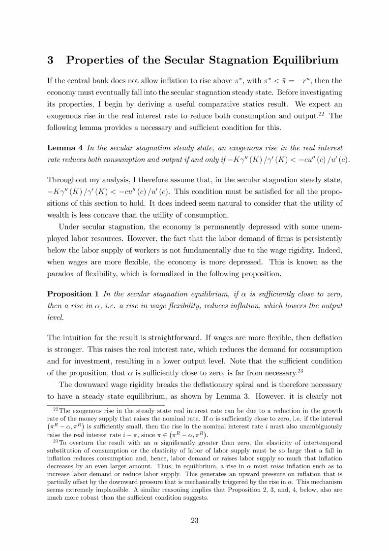
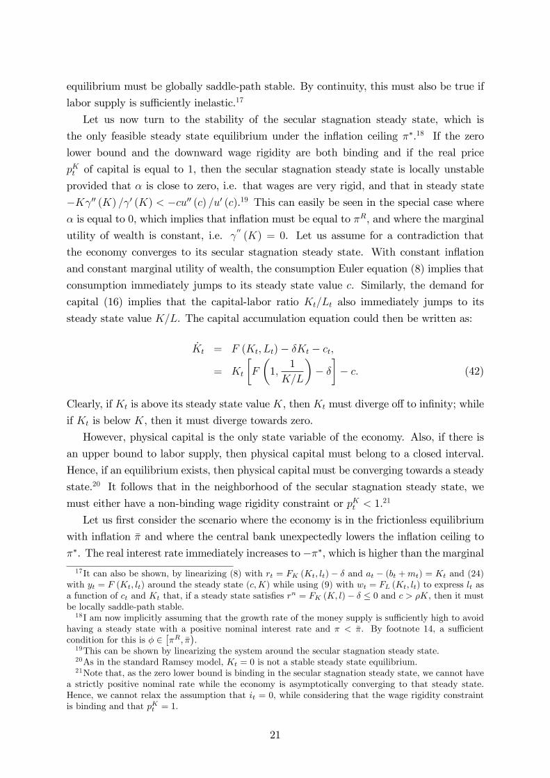
3 Properties of the Secular Stagnation Equilibrium

If the central bank does not allow in�ation to rise above ��, with �� < �� = �rn, then theeconomymust eventually fall into the secular stagnation steady state. Before investigating

its properties, I begin by deriving a useful comparative statics result. We expect an

exogenous rise in the real interest rate to reduce both consumption and output.22 The

following lemma provides a necessary and su¢ cient condition for this.

Lemma 4 In the secular stagnation steady state, an exogenous rise in the real interestrate reduces both consumption and output if and only if �K 00 (K) = 0 (K) < �cu00 (c) =u0 (c).

Throughout my analysis, I therefore assume that, in the secular stagnation steady state,

�K 00 (K) = 0 (K) < �cu00 (c) =u0 (c). This condition must be satis�ed for all the propo-sitions of this section to hold. It does indeed seem natural to consider that the utility of

wealth is less concave than the utility of consumption.

Under secular stagnation, the economy is permanently depressed with some unem-

ployed labor resources. However, the fact that the labor demand of �rms is persistently

below the labor supply of workers is not fundamentally due to the wage rigidity. Indeed,

when wages are more �exible, the economy is more depressed. This is known as the

paradox of �exibility, which is formalized in the following proposition.

Proposition 1 In the secular stagnation equilibrium, if � is su¢ ciently close to zero,then a rise in �, i.e. a rise in wage �exibility, reduces in�ation, which lowers the output

level.

The intuition for the result is straightforward. If wages are more �exible, then de�ation

is stronger. This raises the real interest rate, which reduces the demand for consumption

and for investment, resulting in a lower output level. Note that the su¢ cient condition

of the proposition, that � is su¢ ciently close to zero, is far from necessary.23

The downward wage rigidity breaks the de�ationary spiral and is therefore necessary

to have a steady state equilibrium, as shown by Lemma 3. However, it is clearly not

22The exogenous rise in the steady state real interest rate can be due to a reduction in the growthrate of the money supply that raises the nominal rate. If � is su¢ ciently close to zero, i.e. if the interval��R � �; �R

�is su¢ ciently small, then the rise in the nominal interest rate i must also unambiguously

raise the real interest rate i� �, since � 2��R � �; �R

�.

23To overturn the result with an � signi�cantly greater than zero, the elasticity of intertemporalsubstitution of consumption or the elasticity of labor of labor supply must be so large that a fall inin�ation reduces consumption and, hence, labor demand or raises labor supply so much that in�ationdecreases by an even larger amount. Thus, in equilibrium, a rise in � must raise in�ation such as toincrease labor demand or reduce labor supply. This generates an upward pressure on in�ation that ispartially o¤set by the downward pressure that is mechanically triggered by the rise in �. This mechanismseems extremely implausible. A similar reasoning implies that Proposition 2, 3, and, 4, below, also aremuch more robust than the su¢ cient condition suggests.

23

the friction at the origin of the economic depression. Secular stagnation is instead due

to a lack of demand resulting from the lower bound on the real interest rate. Indeed,

the preference for wealth induces households to have such a high propensity to save that,

in the absence of frictions, a very low real interest rate is necessary to raise aggregate

demand to the level of aggregate supply. In a nutshell, the gap between labor supply and

labor demand is not primarily due to the wage being too high, it is instead due to the

real interest rate being too high.

The in�ation ceiling �� induces the economy to fall into secular stagnation, where the

real interest rate r = �� 2���R;�

��R � �

��is essentially determined by the downward

wage rigidity. At this interest rate, which is actually strictly higher than the lower bound

���, aggregate demand is very weak. Hence, the labor demand L of �rms falls belowthe labor supply l of workers to equate aggregate supply to the weak level of aggregate

demand. Output is essentially demand determined.

To understand why a lack of demand can reduce the output level of the economy, it

is important to realize that a rise in the propensity to save does not necessarily translate

into higher investment. In fact, under secular stagnation, a rise in the intensity of the

preference for wealth reduces investment. This is known as the paradox of thrift, which

is stated in the following proposition.

Proposition 2 In the secular stagnation equilibrium, if � is su¢ ciently close to zero,then a rise in the marginal utility of wealth reduces both consumption and investment.

Indeed, a rise in the propensity to save reduces consumption, which contracts the level

of aggregate demand, which in turn reduces the labor demand of �rms. In the limit as

� tends to zero, the real interest rate remains equal to ��R and the capital-labor ratiomust remain constant. This requires a fall in the capital stock and, hence, in steady

state investment. If � is positive, the reduction in aggregate demand decreases in�ation,

which ampli�es the contraction in both consumption and investment. Thus, a rise in the

marginal utility of wealth lowers the equilibrium level of wealth!

By contrast, in the frictionless equilibrium, a rise in the supply of savings, due to an

increase in the marginal utility of wealth, reduces the equilibrium real interest rate. This

raises the stock of capital. It also raises consumption provided that, initially, the capital

stock is not too high.24 In the absence of frictions, we therefore have the usual result that

a rise in the propensity to save raises investment and the capital stock. The fundamental

24By totally di¤erentiating the equations that characterize the frictionless steady state equilibrium, itcan be shown that a su¢ cient condition to have the capital stock K increasing in the marginal utilityof wealth is that the natural real interest rate is negative (or positive but su¢ ciently close to zero)and either that labor supply is su¢ ciently inelastic or that c > �K. In that case, consumption c isalso increasing in the marginal utility of wealth provided that the natural real interest rate is not toonegative, i.e. provided that the capital stock is not too high.

24

problem under secular stagnation is that the real interest rate is determined by in�ation,

and hence by the downward wage rigidity, rather than by the supply and demand for

loans.

When the economy su¤ers from a lack of demand, expansionary supply shocks can be

contractionary. This is the paradox of toil, which is formalized in the following proposi-

tion.

Proposition 3 In the secular stagnation equilibrium, if � is su¢ ciently close to zero:

� A fall in the disutility of labor reduces consumption, investment and, hence, output;

� Under a Cobb-Douglas aggregate production function, a rise in total factor produc-tivity reduces consumption, investment and, hence, output.

A rise in the supply of labor l, decreases the marginal product of labor at full capacity

FL (K; l). By the binding wage rigidity constraint (33), this reduces the growth rate of

nominal wages and, hence, the in�ation rate. The corresponding rise in the real interest

rate r = �� generates a contraction in the demand for consumption and for investment.The e¤ect of a rise in total factor productivity is slightly more complex. On the

one hand, it mechanically raises the marginal product of capital, which induces �rms to

raise their capital-labor ratio K=L. On the other hand, thanks to higher productivity

and to more capital per worker, the amount of labor L necessary to meet the demand for

consumption falls. It turns out that, with a Cobb-Douglas aggregate production function,

these two e¤ects exactly cancel out and, hence, total factor productivity has no direct

impact on investment �K. However, a higher total factor productivity raises the marginal

product of labor FL (K;L), which increases the labor supply l of workers.25 As before,

this reduces in�ation, which generates a contraction in the demand for consumption and

for investment.

In a nutshell, an expansionary supply shock cannot raise output if it fails to generate

a corresponding increase in aggregate demand. The problem is that, under secular stag-

nation, the real interest rate is determined by in�ation. By contrast, in the frictionless

equilibrium, the real interest rate adjusts such as to equate aggregate demand to aggre-

gate supply. Thus, in the absence of frictions, a rise in the supply of labor induces a fall

in the real interest rate such as to generate a rise in the demand for consumption and for

investment.26

25Recall that, by (9) and (15), we have v0 (l) = FL (K;L)u0 (c).26It can be shown that in the frictionless equilibrium, if the real interest rate is negative (or positive

but su¢ ciently close to zero), c > �K, and �K 00 (K) = 0 (K) < �cu00 (c) =u0 (c), then a fall in thedisutility of labor raises consumption, investment, and output. Also, if the real interest rate is negative(or positive but su¢ ciently close to zero), labor supply is su¢ ciently inelastic, and �K 00 (K) = 0 (K) <�cu00 (c) =u0 (c), then a rise in total factor productivity raises output. Note that these su¢ cient conditionsare far from necessary.

25

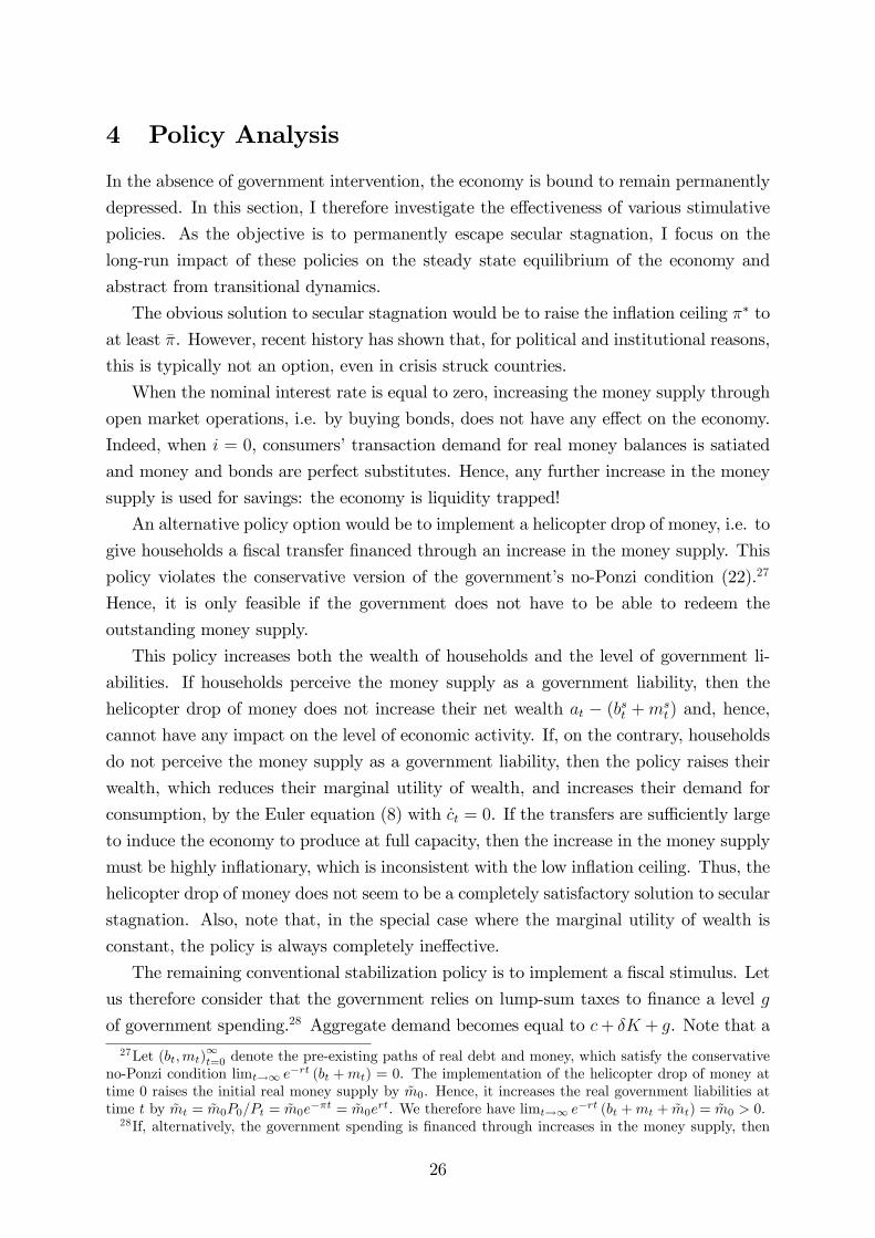
4 Policy Analysis

In the absence of government intervention, the economy is bound to remain permanently

depressed. In this section, I therefore investigate the e¤ectiveness of various stimulative

policies. As the objective is to permanently escape secular stagnation, I focus on the

long-run impact of these policies on the steady state equilibrium of the economy and

abstract from transitional dynamics.

The obvious solution to secular stagnation would be to raise the in�ation ceiling �� to

at least ��. However, recent history has shown that, for political and institutional reasons,

this is typically not an option, even in crisis struck countries.

When the nominal interest rate is equal to zero, increasing the money supply through

open market operations, i.e. by buying bonds, does not have any e¤ect on the economy.

Indeed, when i = 0, consumers�transaction demand for real money balances is satiated

and money and bonds are perfect substitutes. Hence, any further increase in the money

supply is used for savings: the economy is liquidity trapped!

An alternative policy option would be to implement a helicopter drop of money, i.e. to

give households a �scal transfer �nanced through an increase in the money supply. This

policy violates the conservative version of the government�s no-Ponzi condition (22).27

Hence, it is only feasible if the government does not have to be able to redeem the

outstanding money supply.

This policy increases both the wealth of households and the level of government li-

abilities. If households perceive the money supply as a government liability, then the

helicopter drop of money does not increase their net wealth at � (bst +mst) and, hence,

cannot have any impact on the level of economic activity. If, on the contrary, households

do not perceive the money supply as a government liability, then the policy raises their

wealth, which reduces their marginal utility of wealth, and increases their demand for

consumption, by the Euler equation (8) with _ct = 0. If the transfers are su¢ ciently large

to induce the economy to produce at full capacity, then the increase in the money supply

must be highly in�ationary, which is inconsistent with the low in�ation ceiling. Thus, the

helicopter drop of money does not seem to be a completely satisfactory solution to secular

stagnation. Also, note that, in the special case where the marginal utility of wealth is

constant, the policy is always completely ine¤ective.

The remaining conventional stabilization policy is to implement a �scal stimulus. Let

us therefore consider that the government relies on lump-sum taxes to �nance a level g

of government spending.28 Aggregate demand becomes equal to c+ �K + g. Note that a27Let (bt;mt)

1t=0 denote the pre-existing paths of real debt and money, which satisfy the conservative

no-Ponzi condition limt!1 e�rt (bt +mt) = 0. The implementation of the helicopter drop of money at

time 0 raises the initial real money supply by ~m0. Hence, it increases the real government liabilities attime t by ~mt = ~m0P0=Pt = ~m0e

��t = ~m0ert. We therefore have limt!1 e

�rt (bt +mt + ~mt) = ~m0 > 0.28If, alternatively, the government spending is �nanced through increases in the money supply, then

26

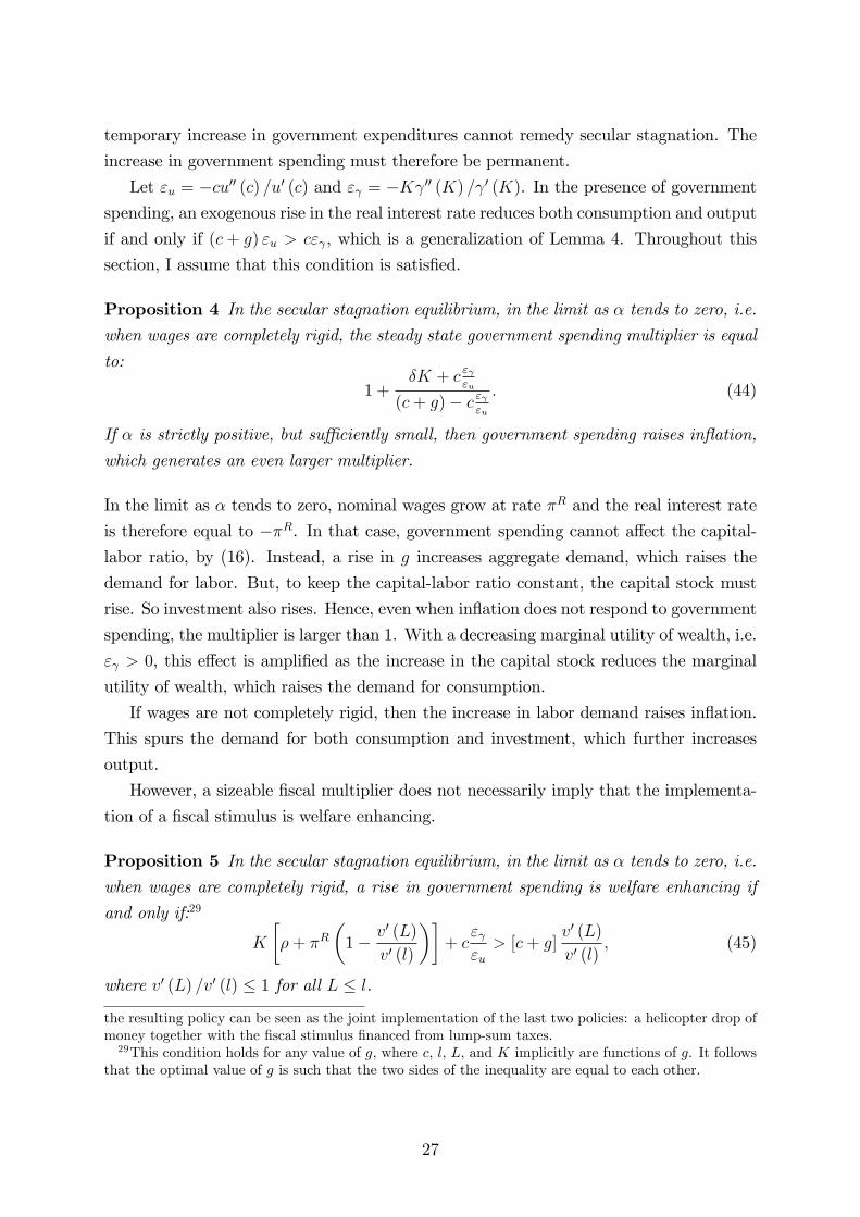
temporary increase in government expenditures cannot remedy secular stagnation. The

increase in government spending must therefore be permanent.

Let "u = �cu00 (c) =u0 (c) and " = �K 00 (K) = 0 (K). In the presence of governmentspending, an exogenous rise in the real interest rate reduces both consumption and output

if and only if (c+ g) "u > c" , which is a generalization of Lemma 4. Throughout this

section, I assume that this condition is satis�ed.

Proposition 4 In the secular stagnation equilibrium, in the limit as � tends to zero, i.e.when wages are completely rigid, the steady state government spending multiplier is equal

to:

1 +�K + c "

"u

(c+ g)� c " "u

: (44)

If � is strictly positive, but su¢ ciently small, then government spending raises in�ation,

which generates an even larger multiplier.

In the limit as � tends to zero, nominal wages grow at rate �R and the real interest rate

is therefore equal to ��R. In that case, government spending cannot a¤ect the capital-labor ratio, by (16). Instead, a rise in g increases aggregate demand, which raises the

demand for labor. But, to keep the capital-labor ratio constant, the capital stock must

rise. So investment also rises. Hence, even when in�ation does not respond to government

spending, the multiplier is larger than 1. With a decreasing marginal utility of wealth, i.e.

" > 0, this e¤ect is ampli�ed as the increase in the capital stock reduces the marginal

utility of wealth, which raises the demand for consumption.

If wages are not completely rigid, then the increase in labor demand raises in�ation.

This spurs the demand for both consumption and investment, which further increases

output.

However, a sizeable �scal multiplier does not necessarily imply that the implementa-

tion of a �scal stimulus is welfare enhancing.

Proposition 5 In the secular stagnation equilibrium, in the limit as � tends to zero, i.e.when wages are completely rigid, a rise in government spending is welfare enhancing if

and only if:29

K

��+ �R

�1� v0 (L)

v0 (l)

��+ c

" "u

> [c+ g]v0 (L)

v0 (l); (45)

where v0 (L) =v0 (l) � 1 for all L � l.

the resulting policy can be seen as the joint implementation of the last two policies: a helicopter drop ofmoney together with the �scal stimulus �nanced from lump-sum taxes.29This condition holds for any value of g, where c, l, L, and K implicitly are functions of g. It follows

that the optimal value of g is such that the two sides of the inequality are equal to each other.

27

A rise in government spending a¤ects welfare through three channels. First, to meet

the higher level of demand, employment L rises. Agents work more, which reduces

their welfare. Second, when wages are rigid, the capital-labor ratio is constant and the

capital stock must therefore rise. This raises the wealth of households, net of government

liabilities, which is welfare enhancing. Finally, if " > 0, the increase in wealth raises the

demand for consumption, which is also welfare enhancing. However, even when g = 0, it

is not clear whether the positive e¤ects dominate.

If labor supply is completely inelastic, then v0 (L) =v0 (l) = 0 for all L < l. This implies

that working more hours whenever L < l is not costly. Hence, increasing g always raises

welfare as long as L < l. This yields the following corollary.

Corollary 1 If labor supply is completely inelastic, then the optimal �scal stimulus elim-inates the gap between labor demand L and labor supply l.

It is important to realize that, even if " = 0, i.e. even if consumption is independent of g,

eliminating under-employment is welfare enhancing as it raises the wealth of households

while the disutility from supplying labor up to l is negligible.

If labor supply is in�nitely elastic, then v0 (L) =v0 (l) = 1. In that case, under the

mild condition that c [1� " ="u] > �K, the implementation of any �scal stimulus is

detrimental to welfare, despite a multiplier that is larger than 1. By continuity, this

result must also hold for a su¢ ciently high elasticity of labor supply.

Corollary 2 If in the secular stagnation equilibrium c [1� " ="u] > �K and if labor

supply is highly elastic, then the implementation of a �scal stimulus reduces welfare.

Thus, starting from a positive level of government spending, it would actually be desirable

to cut government expenditures. This would allow workers to enjoy even more leisure.

Arguably, for plausible calibrations, v0 (L) =v0 (l) is unlikely to be very close to zero,

even when g = 0. For instance, a severe depression, where labor demand is only 75%

of labor supply, together with a Frisch elasticity of labor supply of 0.5 implies that

v0 (L) =v0 (l) = (0:75)1=0:5 = 0:5625. Of course, the case for a �scal stimulus is stronger

if wages are not completely sticky. However, the absence of outright de�ation in almost

any country during the Great Recession suggests that, in practice, in�ation is not very

responsive to government spending. All this suggests that, under secular stagnation, the

case for a �scal stimulus is, at best, weak.

My analysis of the �scal stimulus so far assumes that the economy remains in the sec-

ular stagnation equilibrium. However, an increase in government spending raises the real

interest rate of the frictionless equilibrium.30 Thus, a �scal stimulus that is su¢ ciently

30It can be shown that a su¢ cient condition for this is c+ g � �K and f 0 (k)� � � 0.

28

large to raise the frictionless interest rate from ��� to ��� makes the frictionless equilib-rium consistent with the in�ation ceiling ��. Note that, to implement this equilibrium,

the money supply must be growing at rate ��.

Of course, this policy does not eliminate the secular stagnation equilibrium. The

di¢ culty is to make sure that the economy converges to the frictionless equilibrium. If

this does not spontaneously occur, the government can eliminate the secular stagnation

equilibrium by committing to prevent in�ation from falling below �R. Indeed, at any point

in time, it can always spend su¢ ciently to eliminate the gap between labor demand L and

labor supply l, which raises in�ation to at least �R, by (36). In theory, if this commitment

is fully credible, households expect the economy to converge to the frictionless steady

state with in�ation ��. In practice, it might be very di¢ cult for a government to credibly

commit to spend su¢ ciently to prevent the occurrence of a steady state with under-

employed workers.31

5 Optimal Policy

To lift the economy out of secular stagnation, we clearly need to look beyond the usual

set of policy instruments used for macroeconomic stabilization. Hence, I now characterize

the optimal policy under a much richer set of taxes and subsidies. I proceed in two steps.

First, I determine the optimal allocation of resources. I then solve for the �scal policy

that implements this allocation in the decentralized economy.

5.1 Optimal Allocation

Wealth can either be held in the form of physical capital Kt, bonds bt, or money mt.

Hence, in equilibrium, the private wealth of households net of government liabilities must

be equal to Kt. The planner�s problem is to maximize the welfare of the representative

household: Z 1

0

e��t [u (ct)� v (lt) + h (mt) + (Kt)] dt; (46)

subject to the resource constraint given by the capital accumulation equation:

_Kt = F (Kt; lt)� �Kt � ct; (47)

where I have used the fact that, in a �rst-best allocation, the labor used in production

Lt must be equal to the labor supplied by workers lt. By the maximum principle, for any

31In the late 1930s, Hansen (1939) believed that the U.S. economy was trapped into a secular stagnationequilibrium. A possible interpretation of the subsequent history is that the military spending of WorldWar II allowed the economy to escape secular stagnation, while the build-up of the welfare state afterWWII may have been su¢ cient to allow the economy to produce at full capacity.

29

initial stock K0 of capital, the �rst-best allocation (c�t ; K�t ; l

�t ;m

�t ) is characterized by:

32

_K�t = F (K�

t ; l�t )� �K�

t � c�t ; (48)

_c�tc�t=

�FK (K

�t ; l

�t )� � � �+

0 (K�t )

u0 (c�)

�u0 (c�t )

�u00 (c�t ) c�t; (49)

v0 (l�t ) = FL (K�t ; l

�t )u

0 (c�t ) ; (50)

h0 (m�t ) = 0; (51)

together with the transversality condition:

limt!1

e��tu0 (c�t )K�t = 0: (52)

Money has no impact on the allocation of resources, but is valued by consumers who

derive utility from holding money. Hence, the �rst-best allocation satiates individuals

with real money balances.

These equations correspond to the frictionless equilibrium of the decentralized econ-

omy where consumption is given by (8) with rt = FK (Kt; lt)� � and at� (bt +mt) = Kt,

labor supply by (9) with wt = FL (Kt; lt), and where aggregate supply F (Kt; lt) is equal

to aggregate demand ct + �Kt + _Kt. Also, given the money demand equation (10), to

have h0 (mt) = 0 in a decentralized economy, we need to have it = 0, i.e. the Friedman

(1969) rule needs to hold. This establishes the following result.

Proposition 6 The frictionless equilibrium with it = 0 does implement the �rst-best

allocation of resources.

We have previously established that, under mild conditions, the frictionless steady state

is unique and stable. We can therefore consider that the �rst-best allocation converges

to that steady state.

Let rnt denote the natural real interest rate of the frictionless equilibrium, de�ned as:

rnt = FK (K�t ; l

�t )� �: (53)

Recall that, to have secular stagnation with �� � 0, the steady state natural real interestrate must be negative, i.e. rn = ��� < ��� � 0. This implies that, in the �rst-best

steady state, the capital stock must be above the golden rule level. However, this is fully

e¢ cient as households derive utility from holding real wealth.

32It is straightforward to check that the Hamiltonian is strictly concave in ct, lt, mt, and Kt and thatthe corresponding current-value costate variable is equal to u0 (ct) and that it is therefore always strictlypositive. Hence (by Acemoglu 2009, Theorem 7.14, page 257), for a given value of K0, the optimalityconditions de�ne the unique solution to the optimal control problem.

30

5.2 Implementation in the Decentralized Economy

For simplicity, �rms are assumed to rent capital owned by households. As investment is

always positive in the �rst-best allocation that I want to implement, I assume that the

price of capital is always equal to that of consumption goods, i.e. pKt = PKt =Pt = 1.

A capital income tax �Kt is imposed on the income from physical capital RtKt net of a

depreciation allowance 't�PtKt, where, as before, Rt denotes the nominal rental cost of

capital.33 Under full depreciation allowance, we have 't = 1. There is an investment sub-

sidy sIt . As we shall see, this reduces the e¤ective price of capital at time t to Pt�1� sIt

�.

The e¤ective nominal wealth of a household is therefore equal to:

At =�1� sIt

�PtKt +Bt +Mt: (54)

This wealth is taxed at rate �Wt at each point in time.34 Finally, households are subject

to a labor income tax �Lt and to a consumption tax �Ct .

This �scal policy implies that the nominal wealth PtKt+Bt+Mt of the representative

household evolves according to:

Pt _Kt + _PtKt + _Bt + _Mt (55)

= itBt +�RtKt � �Kt [RtKt � 't�PtKt] + sIt

hPt _Kt + �PtKt

i� �PtKt + _PtKt

���Wt

��1� sIt

�PtKt +Bt +Mt

�+�1� �Lt

�Wtlt + Pt t �

�1 + �Ct

�Ptct;

where nominal investment is equal to Pt _Kt+�PtKt. Using the fact that _Bt=Pt = _bt+�tbtand _Mt=Pt = _mt + �tmt, this can be written in real terms as:�

1� sIt�_Kt � _sItKt + _bt + _mt =

�it � �t � �Wt

� ��1� sIt

�Kt + bt +mt

�(56)

+��1� �Kt

�Rt=Pt + �Kt 't� �

�1� sIt

�� � _sIt �

�1� sIt

�(it � �t)

�Kt

�itmt +�1� �Lt

�wtlt + t �

�1 + �Ct

�ct:

This expression does con�rm that the e¤ective real price of capital is�1� sIt

�. By

arbitrage, the returns from holding capital should be identical to the returns from holding

bonds. Thus, the second term on the right hand side of (56) must be equal to zero, which

yields the following relationship between the real interest rate and the user cost of capital:

rt =

�1� �Kt

�Rt=Pt + �Kt 't� � _sIt1� sIt

� �: (57)

33If �rms were the owners of capital, then �Kt would correspond to a corporate income tax.34In the optimal allocation, the nominal return from wealth is equal to zero and the real return is

negative (as, in steady state, rn < ��� � 0). Hence, in that context, it seems more natural to tax thestock of wealth rather than the (negative) income from wealth.

31

The wealth accumulation equation simpli�es to:

_at =�rt � �Wt

�at � itmt +

�1� �Lt

�wtlt + t �

�1 + �Ct

�ct; (58)

where at = At=Pt. The corresponding no-Ponzi condition is:

limt!1

e�R t0(rs��Ws )dsat � 0: (59)

Finally, households�intertemporal utility is given by:

Z 1

0

e��t

"u (ct)� v (lt) + h

�mt

1 + �Ct

�+

at �

�bst +ms

t � sItKt

�1 + �Ct

!#dt; (60)

where I assume that they care about the value of money and wealth at consumer prices,

including consumption taxes. The sum of the wealth of the private and of the public

sector must always be equal to the stock of physical capital. Hence, the government

liabilities at t are equal to bst +mst � sItKt, where bst , m

st , and Kt are aggregate quantities

that are outside the control of any single household.

The consumer�s problem is to maximize utility, (60), subject to the budget constraint,

(58) and (59), with a0 given. The solution to the problem is characterized by:

_ctct=

"rt � �Wt �

_�Ct1 + �Ct

� �+1

u0 (ct) 0

at �

�bst +ms

t � sItKt

�1 + �Ct

!#u0 (ct)

�u00 (ct) ct; (61)

v0 (lt) =1� �Lt1 + �Ct

wtu0 (ct) ; (62)

h0�

mt

1 + �Ct

�= itu

0 (ct) ; (63)

together with the transversality condition:

limt!1

e��tu0 (ct)

1 + �Ctat = 0: (64)

The reason why _�Ct appears in the Euler equation (61) is that a rising path of the con-

sumption tax makes future consumption expansive relative to current consumption. This

reduces the e¤ective real interest rate faced by consumers, which raises the demand for

consumption.

On the supply side, the constant returns to scale production function implies that, in

32

equilibrium, the real rental cost of capital and the real wage are given by:

RtPt

= FK (Kt; Lt) ; (65)

wt = FL (Kt; Lt) ; (66)

respectively.

The downward wage rigidity is the same as before, summarized by (36). As the

�rst-best allocation is characterized by full employment, i.e. Lt = lt, it cannot be imple-

mented with in�ation below �R. Thus, as we shall see, the �rst-best allocation can be

implemented for any given path of in�ation such that �t 2��R; ��

�. This requires the

money supply to grow at rate �t at time t.

In the �rst-best allocation, households have a zero marginal utility of real money

balances, by (51). The decentralized money demand equation (63) therefore implies that,

to implement the optimal allocation, we must have it = 0 and, hence, rt = ��t.Fundamentally, in the laissez-faire economy, the lower bound on the real interest rate,

rt � ���, creates two distortions that need to be corrected. First, by (8), it reduces thedemand for consumption. Second, by (16), it reduces the capital-labor ratio.

To correct the �rst distortion, the net-of-tax interest rate rt � �Wt � _�Ct =�1 + �Ct

�=

��t � �Wt � _�Ct =�1 + �Ct

�in the demand for consumption (61) must be equal to the

natural real interest rate rnt . As in practice the consumption tax cannot be increasing

forever, I impose that it must be constant over time, i.e. _�Ct = 0. To implement the

�rst-best allocation for a given �t 2��R; ��

�, the wealth tax must therefore be given by:

�Wt = �rnt � �t: (67)

This guarantees that the consumption Euler equation of the decentralized economy (61)

coincides with the corresponding �rst-order condition to the planner�s problem (49). Sec-

ular stagnation results from the fact that in steady state rnt = rn < ���, which impliesthat �Wt = �rn � �t > �� � �t � 0.To correct the second distortion, the marginal product of capital of the frictionless

equilibrium FK (K�t ; l

�t ) = � + rnt must be made consistent with real interest rate of the

decentralized economy rt = ��t. Hence, by the arbitrage relationship (57), the capitalincome tax �Kt , the depreciation allowance 't, and the investment subsidy s

It must be

jointly chosen such that:

��t =�1� �Kt

�[� + rnt ] + �Kt 't� � _sIt1� sIt

� �: (68)

Let us consider three special cases of interest. For simplicity, I focus on the optimal policy

33

with constant in�ation � 2��R; ��

�and in steady state, where rnt = rn = ���. First,

relying exclusively on the investment subsidy, i.e. �K = 0, we have:

sI =�rn � �

� � �; (69)

which is strictly positive, as rn < ��� � �� and ��� > ���� = �+rn = FK (K�; l�) > 0.

Second, relying on the capital income tax with full depreciation allowance, i.e. sI = 0

and ' = 1, we obtain:

�K =�rn � �

�rn ; (70)

which is strictly positive (to the extent that �� � 0 implies rn < 0). In fact, the

negative natural real interest rate implies that the returns from capital in the frictionless

equilibrium are negative. Hence, with full depreciation allowance, a positive capital

income tax absorbs some of the losses from capital. It therefore subsidizes capital. Third,

relying again on the capital income tax but with no depreciation allowance, i.e. sI = 0

and ' = 0, we have:

�K =rn + �

� + rn; (71)

which, in steady state, is negative as rn + � = ��� + � < 0. With no depreciation

allowance, the capital income tax needs to be negative to subsidize capital. Importantly,

these three policies are equivalent as they all implement the same marginal product of

capital rn + � = FK (K�; l�).

The optimality condition for labor supply (50) implies that, if both consumption and

the capital-labor ratio are at their �rst-best levels, then so is the supply of labor. Hence,

by (62) and (66), the labor income and consumption taxes can both be set equal to zero,

i.e. �Lt = �Ct = 0.

Let us now determine the level of the lump-sum transfers t that balances the in-

tertemporal government budget constraint. The accumulation of government liabilities

is given by:

_bst + _mst = rt [b

st +ms

t ]� itmst + t + sIt

h_Kt + �Kt

i� �Kt [Rt=Pt � 't�]Kt � �Wt at: (72)

Rearranging terms, this can be written as:

_bst + _mst � sIt

_Kt � _sItKt =�rt � �Wt

� �bst +ms

t � sItKt

�(73)

�itmst + t + sIt [rt + �]Kt � _sItKt � �Kt [Rt=Pt � 't�]Kt � �Wt Kt:

But, by the arbitrage relationship (57), we know that sIt [rt + �]� _sIt ��Kt [Rt=Pt � 't�] =

rt + � � Rt=Pt. As the sum of the wealth of the private and of the public sector must

be equal to the stock of physical capital, the government is always solvent, and able to

34

redeem the money supply, provided that it satis�es the following no-Ponzi condition:35

limt!1

e�R t0(rs��Ws )ds

�bst +ms

t � sItKt

�� 0: (74)

Hence, the government�s intertemporal budget constraint is given by:

b0 +m0 � sI0K0 (75)

+

Z 1

0

e�R t0(rx��Wx )dx

��itms

t + t + (rt + � �Rt=Pt)Kt � �Wt Kt

�dt � 0;

But, in the �rst-best allocation, it = 0. Also, the optimal policy for a given �t 2��R; ��

�is such that rt = ��t, Rt=Pt � � = rnt and �

Wt = �rnt � �t. It immediately follows that

the government budget constraint simpli�es to:

b0 +m0 � sI0K0 +

Z 1

0

e�R t0 r

nxdx tdt � 0: (76)

This shows that, if sI0 = 0, the optimal policy is self-�nancing as the wealth tax pays

for the subsidization of income from physical capital. The only e¤ect of the policy is to

modify the real interest rate at which future lump-sum transfers are discounted.

The initial investment subsidy sI0 reduces the initial price of capital, which tightens

the budget constraint of households. This mechanically relaxes the government budget

constraint. Hence, sI0 acts as a levy on initial capital. However, if the natural real interest

rate rnt is eventually negative, then in�nitesimally small negative lump-sum transfers tforever are su¢ cient to balance the government budget constraint for any �nite value of

sI0. In that case, the lump-sum transfers that the government can a¤ord are not a¤ected

by sI0.

Proceeding as before, cf. (41), it is straightforward to check that, under the optimal

policy, the transversality conditions of the household (64) and of the planner (52) coincide.

We have therefore characterized by construction a policy that can implement the �rst-

best allocation for any path of in�ation such that �t 2��R; ��

�at all time t. The main

result is summarized in the following proposition.

Proposition 7 At any time T , the �rst-best allocation can be implemented in the decen-tralized economy for any given path of in�ation (�̂t)

1t=T such that �̂t 2

��R; ��

�for all

t � T by setting the money growth rate �t, the tax on wealth �Wt , the capital income tax

35This is a generalization of the conservative government budget constraint, given by (22).

35

�Kt , the depreciation allowance 't, and the investment subsidy sIt such that:

�t = �̂t; (77)

�Wt = �rnt � �̂t; (78)�1� sIt

�[� � �̂t] =

�1� �Kt

�[� + rnt ] + �Kt 't� � _sIt : (79)

This policy is revenue neutral, except that sI0 acts as a levy on initial capital.

The optimal policy implements the allocation of the frictionless equilibrium with it = 0.

However, it implements this allocation with in�ation �t = �̂t 2��R; ��

�, rather than the

much higher rate �t = �rnt .By construction, the optimal policy is consistent with the in�ation ceiling �� at all

time, except possibly when the policy is implemented. Indeed, as the economy jumps

from the secular stagnation to the frictionless equilibrium, the zero lower bound ceases

to bind.36 If the policy is implemented at time T with it = 0, then the price level at T

must be given by:

PT =MT

�m.

To prevent the price level from jumping upon implementation of the policy, the money

supply at time T must be equal to �mPT�", where PT�" denotes the price level that pre-

vailed just before. If the real money supply at time T � " was larger than the transactiondemand for money, i.e. mT�" > �m, the government must redeem a quantity mT�" � �m

of money. This can generate a massive increase in government debt.37 However, in the-

ory, with a permanently negative natural real interest rate, the government�s no-Ponzi

condition (74) is satis�ed for an arbitrarily large initial level of debt, provided that the

primary budget is subsequently balanced. These considerations nevertheless show that, if

the government used to rely excessively on the printing press to �nance its expenditures,

then the sustainability of public debt can become an important issue when the optimal

policy is implemented.

For simplicity, let us consider that the government targets a constant rate of in�ation

�̂ 2��R; ��

�and that, once the economy is in steady state, the policy becomes time

36Even if the nominal interest rate remains equal to zero, the zero lower bound is no longer preventingthat rate from being negative. Hence, as explained in the derivation of the steady state equilibrium, anequilibrium where some money is used for saving is unstable.37In my model, the government corresponds to the consolidation of the ministry of �nance and of the

central bank. In practice, the central bank can redeem the money supply by selling the governmentbonds that it previously acquired to �nance the public de�cit. This does not change the indebtednessof the ministry of �nance, but raises the amount of debt held by the private sector rather than by thecentral bank. In Japan, the debt-to-GDP ratio amounts to 230% of GDP, a quarter of which is held bythe central bank. Thus, the amount of debt held by the private sector only amounts to 170% of GDP. IfJapan escapes the liquidity trap, this ratio would need to increase sharply to avoid a jump in the pricelevel.

36

invariant, i.e. �t = �, �Wt = �W , �Kt = �K , 't = ', and sIt = sI . Importantly, the

optimal policy does not eliminate the secular stagnation equilibrium, where in�ation is

below the target �̂.38 There is however one important exception.

Proposition 8 The frictionless and secular stagnation steady state equilibria can coin-cide if and only if the optimal policy is implemented with in�ation target �̂ = �R. If the

secular stagnation equilibrium is unique, which must be the case for � su¢ ciently close

to zero, then the optimal policy with �̂ = �R uniquely implements the �rst-best allocation.

Implementing the optimal allocation with in�ation target �̂ = �R requires the most

aggressive policy intervention, i.e. the largest wealth tax and the highest subsidization

of physical capital. Indeed, a massive intervention is necessary to make the optimal

allocation consistent with an in�ation rate as low as �R.

If the government would like to be in the optimal allocation with in�ation ��, then

it should �rst implement the optimal policy with �̂ = �R in order to escape secular

stagnation. It should then raise the growth rate of the money supply to ��, while reducing

the size of the wealth tax, and of the subsidization of capital that it �nances, until the

nominal interest rate is back to zero.

The wealth of households is composed of physical capital, bonds, and money. A

potential concern with the optimal policy is that money might be harder to tax than

physical capital or bonds. Households might indeed be tempted to accumulate stockpiles

of cash to avoid paying the wealth tax. But, untaxed money yields a real interest rate

��t, which, under the in�ation ceiling, is higher than the steady state natural real interestrate. By arbitrage, this would induce the after-tax real interest rate on physical capital

and on bonds to be above the natural rate, which would prevent the implementation of

the optimal allocation. It is therefore essential that the government is able to tax money.

To �ght against money laundering, many countries already enforce signi�cant restric-

tions that reduce the value of large sums of undeclared currency. There are limits to the

size of payments than can be made in cash.39 Banks cannot accept large cash deposits if

the origin of the funds is not proven. Controls can also be made when old bills occasion-

ally become obsolete and are replaced by new ones. If these measures are not su¢ cient,

then the government can adopt a payment system that exclusively relies on electronic

money.

Note that, if money is straightforward to tax, then an alternative way to implement

the �rst-best allocation is to alleviate the zero lower bound on the nominal interest rate.

For this, a government targeting in�ation �̂t only needs to tax money at rate �Wt , while

38Note that, the optimal policy is revenue neutral even if it fails to implement the optimal allocation.39In France, the limit is 1 000 euros for commercial transactions and 10 000 euros for real estate

transactions.

37

setting the money growth rate �t and the tax rate on money �Wt according to (77) and

(78), respectively. The lower bound on the nominal interest rate becomes ��Wt , which isnegative. In that case, when the nominal rate is at its lower bound, the real interest rate

is at its natural level, as it = ��Wt = rnt + �̂t implies rt = it � �̂t = rnt . This policy is

revenue neutral.

In the absence of electronic money, the tax on wealth seems to o¤er a more reliable

way to reduce the net-of-tax real interest rate faced by households than the tax on

money. Indeed, the wealth tax is e¤ective provided that the authorities can prevent large

accumulations of undeclared currency. By contrast, if real money balances are small

and the tax on money is poorly enforced on small amounts, then it is not clear that,

by arbitrage, it can reduce the net-of-tax real interest rate faced by households on their

holdings of physical capital and bonds. This suggests that, without electronic money, it

is likely to be very di¢ cult to enforce negative nominal interest rates.

6 Heterogeneity

For simplicity, I have so far relied on a representative household model. However, my

results only require a strictly positive mass of households to have a preference for wealth.

Indeed, in the presence of heterogeneity, impatient households borrow from those who are

more patient, until they reach their borrowing limit. Once this limit is reached, the real

interest rate must be su¢ ciently low to induce the most patient households to consume

enough to allow the economy to produce at full capacity. In other words, in steady state,

the natural real interest rate must be determined by the behavior of the most patient

households, i.e. by those who have a preference for wealth.

Under a dynastic interpretation of the in�nitely lived households, the borrowing limit

should be determined by the impossibility of bequeathing negative wealth. For instance,

in a discrete time model where one period corresponds to one generation, households

face a zero debt limit. As the borrowing limit must eventually be binding, I consider a

very simple form of heterogeneity whereby a fraction of households have a preference for

wealth, while the remaining fraction consists of hand-to-mouth consumers who do not

derive any utility from holding wealth.

Interestingly, in this setup, if the real interest rate is excessively high, then the econ-

omy can only produce at full capacity if poor households accumulate an excessive amount

of debt. But, once the rich lenders realize that debt cannot be passed on to the next

generation of poor households, the economy has to go through a painful deleveraging

episode. As pointed out by Summers (2014), the fact that the credit boom that occurred

before the Great Recession did not overheat the U.S. economy is fully consistent with the

secular stagnation hypothesis.

38

In the presence of heterogeneity, the government might want to redistribute resources

across households. In general, as in Correia, Farhi, Nicolini and Teles (2013), the set of

implementable allocation is not modi�ed by the zero lower bound. Indeed, the government

can always implement its desired redistribution policy, while using wealth taxes and

investment subsidies as described in the previous section to overcome the zero lower

bound.40

In the context of secular stagnation, there is however one important exception where

the zero lower bound can allow the government to implement an allocation that would

not otherwise be feasible. This occurs when the government would like to redistribute

to hand-to-mouth households, but cannot rely on household-speci�c lump-sum taxes or

subsidies and does not want to modify the tax rate on wealth, as this would distort the

consumption behavior of wealthy households.41 Hence, the government can only raise the

consumption of the hand-to-mouth by giving a lump-sum subsidy t to all households.

If t is large, this clearly violates the conservative government budget constraint, given

by:

b0 +m0 +

Z 1

0

e�R t0 rxdx [ t � itmt] dt � 0: (80)

But, if the government does not need to redeem the outstanding money supply, the budget

constraint becomes:

b0 +

Z 1

0

e�R t0 rxdx [ t � �tmt] dt � 0: (81)

The subsidy can be �nanced by printing money forever. The wealth of rich households

must therefore grow without bounds. Indeed, if the conservative version of the govern-

ment�s no-Ponzi condition is violated and if markets clear, then, by Walras� law, the

no-Ponzi condition of rich households must be slack, for any value of the real interest

rate. The increase in wealth is not distortionary, i.e. it does not a¤ect the behavior of

rich households, provided that it does not change their marginal utility of wealth. This

either occurs if they consider money as a government liability, or if they have a constant

marginal utility of wealth.

Thus, in the absence of household speci�c lump-sum taxes, the only way to redistribute

to the poor without increasing the tax rate on wealth is to print money. This policy can be

sustained forever provided that the wealthy have a zero marginal propensity to consume

out of extra money supplied.42 Paradoxically, this egalitarian allocation of consumption

can only be implemented by making the rich in�nitely wealthy.

40Under secular stagnation, it might be tempting to stimulate aggregate demand by taxing the wealthyand giving lump-sum subsidies to hand-to-mouth households. However, if this is not optimal in theabsence of the zero lower bound, then it remains suboptimal with it.41Given the limited amount of heterogeneity in the model, a non-linear wealth tax could act as a

lump-sum tax. I therefore assume that this instrument is not available.42This assumption does not seem outrageous in light of the recent Japanese experience, where a 230%

debt-to-GDP ratio fails to lift the economy out of secular stagnation.

39

This theoretical possibility is speci�c to secular stagnation where the zero lower bound

is potentially binding forever. Needless to emphasize that such policy is very dangerous

should the economy ever escape secular stagnation. Hence, crucially, the increase in the

consumption of the hand-to-mouth should not induce the economy to produce at full

capacity, as in�ation would then explode.

7 Conclusion

In this paper, I have relied on a Ramsey model with money to o¤er a simple theory of

secular stagnation. The permanent failure of the economy to produce at full capacity

results from three plausible assumptions: (i) the central bank has a low in�ation ceiling;

(ii) a positive mass of households has a very high propensity to save, due to a preference

for wealth; (iii) wages are downward rigid. Despite the simplicity of this theory, I was

able to derive the main Keynesian paradoxes.

I have argued that traditional monetary and �scal policies are not e¢ cient in the

context of a permanent liquidity trap. To escape secular stagnation without raising the

in�ation ceiling, the government should instead simultaneously tax wealth and subsidize

income from physical capital, either through an investment subsidy or a reduction in the

taxation of corporate income. This policy is revenue neutral and implements the �rst-best

allocation of resources.

When the economy escapes the liquidity trap, households cease to rely on money

for saving. To prevent the price level from jumping upon implementation of the opti-

mal policy, the government must therefore shrink the money supply to the level of the

transaction demand for money. This can signi�cantly raise the debt-to-GDP ratio. In

theory, an arbitrarily large amount of public debt is sustainable when the real interest

rate is negative forever. But, in practice, a country that used to heavily rely on monetary

�nancing of public de�cits might be reluctant to implement the optimal policy. Hence,

an excessive reliance on the printing press can eventually result in a country choosing to

remain permanently trapped into secular stagnation.

References

[1] Acemoglu, D. (2009), Introduction to Modern Economic Growth, Princeton, NJ:

Princeton University Press.

[2] Benhabib, J., Schmitt-Grohé and Uribe (2001), �The Perils of Taylor Rules�, Journal

of Economic Theory, 96, 40-69.

40

[3] Benigno, G. and Fornaro, L. (2015), �Stagnation Traps�, working paper, London

School of Economics and CREI.

[4] Buiter, W.H. (2014), �The Simple Analytics of Helicopter Money: Why It Works

- Always�, Economics: The Open-Access, Open-Assessment E-Journal, 8 (2014-28),

1-51.

[5] Caballero, R.J. and Farhi, E. (2015), �The Safety Trap�, working paper, Harvard and

MIT.

[6] Carroll, C.D. (2000), �Why Do the Rich Save So Much?�, in Does Atlas Shrug? The

Economic Consequences of Taxing the Rich, edited by Joel B. Slemrod, Cambridge,

MA: Harvard University Press.

[7] Correia, I, Farhi, E., Nicolini, J.P. and Teles, P. (2013), �Unconventional Fiscal Policy

at the Zero Bound�, American Economic Review, 103(4), 1172-1211.

[8] Eggertsson, G.B. (2010), �What Fiscal Policy is E¤ective at Zero Interest Rates?�,

in NBER Macroeconomics Annual 2010, edited by Daron Acemoglu and Michael

Woodford, Cambridge, MA: MIT Press.

[9] Eggertsson, G.B. and Mehrotra, N.R. (2014), �A Model of Secular Stagnation�, work-

ing paper, Brown and Columbia.

[10] Eggertsson, G.B. and Woodford, M. (2003), �The Zero Bound on Interest Rates and

Optimal Monetary Policy�, Brookings Papers on Economic Activity, 34(1), 139-235.

[11] Friedman, M. (1969), �The Optimum Quantity of Money�, in The Optimum Quantity

of Money and Other Essays, edited by Milton Friedman, Chicago: Aldine.

[12] Hansen, A. (1939), �Economic Progress and Declining Population Growth�, American

Economic Review, 29(1), 1-15.

[13] Keynes, J.M. (1936), The General Theory of Employment, Interest and Money, Lon-

don: MacMillan Press.

[14] Kocherlakota, N. (2013), �Impact of Land Price Fall When Labor Markets are In-

complete�, working paper, Federal Reserve Bank of Minneapolis.

[15] Kocherlakota, N. and Phelan, C. (1999), �Explaining the Fiscal Theory of the Price

Level�, Federal Reserve Bank of Minneapolis Quarterly Review, 23(4), 14-23.

[16] Kopczuk, W. (2007), �Bequest and Tax Planning: Evidence from Estate Tax Re-

turns�, Quarterly Journal of Economics, 122(4), 1801-1854.

41

[17] Kopczuk, W. (2009), �Economics of Estate Taxation: A Brief Review of Theory and

Evidence�, Tax Law Review, 63(1), 139-157.

[18] Krugman, P. (1998), �It�s baaack: Japan�s Slump and the Return of the Liquidity

Trap�, Brookings Papers on Economic Activity, 29(2), 137-205.

[19] Kumhof, M., Rancière, R. and Winant, P. (2015), �Inequality, Leverage, and Crises�,

American Economic Review, 105(3), 1217-1245.

[20] Michaillat, P., and Saez, E. (2015), �An Economical Business-Cycle Model�, working

paper, LSE and Berkeley.

[21] Obstfeld, M. and Rogo¤, K. (1983), �Speculative Hyperin�ations in Maximizing

Models: Can We Rule Them Out?�, Journal of Political Economy, 91(4), 675-687.

[22] Piketty, T. (2011), �On the Long-Run Evolution of Inheritance: France 1820-2050�,

Quarterly Journal of Economics, 126(3), 1071-1131.

[23] Summers, L.H. (2014), �Re�ections on the �New Secular Stagnation Hypothesis�, in

Secular Stagnation: Facts, Causes and Cures, edited by Coen Teulings and Richard

Baldwin, London: CEPR Press.

[24] Werning, I. (2012), �Managing a Liquidity Trap: Monetary and Fiscal Policy�, work-

ing paper, MIT.

A Proof of Lemma 1

Let k = K=L and f (k) = F (k; 1). This implies that FK (K;L) = f 0 (k) and FL (K;L) =

f (k)� kf 0 (k). Note that f (0)� 0f 0 (0) = FL (0; L) = 0 as F (0; L) = 0 for any value of

L.

In a frictionless equilibrium with � � �� > �R, the labor market must clear, i.e. L = l.

The goods market clearing condition (24) implies that:

l [f (k)� �k] = c: (A1)

By (9) and (15), we have:

v0 (l) = [f (k)� kf 0 (k)]u0 (c) : (A2)

Finally, by (8) with _ct = 0 and at � (bt +mt) = K = kl and by (16), we have:

u0 (c) = 0 (kl)

�� [f 0 (k)� �]. (A3)

42

These three equations jointly characterize the steady state frictionless equilibrium.

Let k̂ be uniquely de�ned by f(k̂) = �k̂. Substituting (A1) into (A2) yields:

v0�

c

f (k)� �k

�= [f (k)� kf 0 (k)]u0 (c) : (A4)

For any given value of k 2 (0; k̂), as c increases from 0 to+1, the right hand side decreasesfrom +1 to 0 while the left hand side is increasing and non-negative. Hence, for any

value of k 2 (0; k̂), there is a unique corresponding value of c. Moreover, di¤erentiating(A4) with respect to k reveals that c is a continuous function of k for k 2 (0; k̂). Also, inthe limit as k tends to k̂, c must tend to 0.43

Let ~k be uniquely de�ned by � = f 0(~k) � �. Clearly, f 0(k̂) � � < 0 < � = f 0(~k) � �.

Hence, ~k < k̂. Substituting (A1) into (A3) yields:

0�

kc

f (k)� �k

�= [�+ � � f 0 (k)]u0 (c) : (A5)

Note that k= [f (k)� �k] is an increasing function of k.44 Let �c be de�ned by [� + � �f 0(k̂)]u0 (�c) = limK!+1

0 (K). Thus, as k tends to k̂ from below, c tends to �c.45 For

any given value of c 2 (0; �c), as k increases from ~k to k̂, the right hand side of (A5)

increases from 0 to [� + � � f 0(k̂)]u0 (c) > [� + � � f 0(k̂)]u0 (�c) while the left hand side

is weakly decreasing and tends to limK!+1 0 (K) = [� + � � f 0(k̂)]u0 (�c) as k tends to

k̂. Hence, for any value of c 2 (0; �c), there is a unique corresponding value of k 2 (~k; k̂).Moreover, di¤erentiating (A5) with respect to c reveals that k is a continuous function

of c for c 2 (0; �c).The steady state frictionless equilibrium is fully characterized by (A4) and (A5). But,

by (A4), c is a continuous function of k for k 2 (0; k̂), which tends to 0 as k tends to k̂;while, by (A5), k is a continuous function of c for c 2 (0; �c) with k 2 (~k; k̂). Hence, thereexists at least one value of k 2 (~k; k̂) that corresponds to a frictionless equilibrium.If � = 0, then we have f 0(~k)� � = 0. If labor supply is inelastic, then, by (A1), c is a

strictly decreasing function of k for all k 2 (~k; k̂), while, by (A3), c is a strictly increasingfunction of k for all k 2 (~k; k̂). Hence, the equilibrium value of k 2 (~k; k̂) must be unique.By continuity, the results also holds provided that � is su¢ ciently small and that labor

supply is su¢ ciently inelastic.

43If the maximum feasible labor supply �l is �nite, then, by (A1), c must tend to 0 while, by (A2), lmust tend to �l, as liml!�l v

0 (l) =1. If �l is in�nite, then c cannot tend to a strictly positive value, as, by(A2), l would also tend to a �nite value which would be inconsistent with (A1). Hence, c must tend to0 while l must tend to 1.44Its derivative is equal to [f (k)� kf 0 (k)] = [f (k)� �k]2, which is positive as f (k) � kf 0 (k) =

FL (K;L).45Note that c cannot tend to 0 as limK!0

0 (K) <1.

43

B Proof of Lemma 2

As in the proof of the previous lemma, let k = K=L and f (k) = F (k; 1). To prove

the lemma, we compare the slope of the aggregate demand and of the aggregate supply

curves. For this, we �rst need to compute the derivative of c, k, and l with respect to r,

where r = i� � with i � 0. Recall that, when � 2��R; ��

�, the labor market clears, i.e.

L = l.

From the equation for the demand for capital (16), we have:

dk

dr=

1

f 00 (k)< 0:

Implicitly di¤erentiating the optimality condition for labor supply (9) with w = f (k)�kf 0 (k) yields:

dl

dr=

1

v00 (l)

��kf 00 (k)u0 (c) dk

dr+ wu00 (c)

dc

dr

�;

=1

v00 (l)

��ku0 (c) + wu00 (c)

dc

dr

�:

Finally, from the optimality condition for consumption (8) with _ct = 0 and at�(bt +mt) =

K = kl, we have:

dc

dr=

1

u00 (c)

� 0 (kl)

(�� r)2+ 00 (kl)

�� r

�ldk

dr+ k

dl

dr

��;

=u0 (c)

u00 (c)

�u0 (c)

0 (kl)+ 00 (kl)

0 (kl)

�l

f 00 (k)+

k

v00 (l)

��ku0 (c) + wu00 (c)

dc

dr

���;

=u0 (c)

u00 (c)

�u0 (c)

0 (kl)� kl 00 (kl)

0 (kl)

�ku0 (c)

lv00 (l)� 1

kf 00 (k)

��+kl 00 (kl)

0 (kl)

v0 (l)

lv00 (l)

dc

dr:

where I have used the fact that � � r = 0 (kl) =u0 (c) to derive the second line and that

wu0 (c) = v0 (l) to derive the third line. Rearranging terms, this expression can be written

as:

dc

dr=

�1lv00(l)v0(l) +

�kl 00(kl) 0(kl)

lv00 (l)

v0 (l)

u0 (c)

�u00 (c)

�u0 (c)

0 (kl)+�kl 00 (kl) 0 (kl)

�ku0 (c)

lv00 (l)+

1

�kf 00 (k)

��;

which shows that consumption is unambiguously decreasing in the real interest rate.

44

Substituting this expression into the derivative of labor supply yields:

dl

dr=

�ku0 (c)v00 (l)

+l

lv00(l)v0(l) +

�kl 00(kl) 0(kl)

�u0 (c)

0 (kl)+�kl 00 (kl) 0 (kl)

�ku0 (c)

lv00 (l)+

1

�kf 00 (k)

��;

=l

lv00(l)v0(l) +

�kl 00(kl) 0(kl)

�u0 (c)

0 (kl)� lv00 (l)

v0 (l)

ku0 (c)

lv00 (l)+�kl 00 (kl) 0 (kl)

1

�kf 00 (k)

�;

=1

lv00(l)v0(l) +

�kl 00(kl) 0(kl)

�lu0 (c)

0 (kl)

�1� k 0 (kl)

v0 (l)

�+�kl 00 (kl) 0 (kl)

l

�kf 00 (k)

�:

But, as 0 (kl) = (�� r)u0 (c) = (�� f 0 (k) + �)u0 (c) and v0 (l) = wu0 (c), we have:

dl

dr=

1lv00(l)v0(l) +

�kl 00(kl) 0(kl)

�lu0 (c)

0 (kl)

�1� k (�� f 0 (k) + �)

w

�+�kl 00 (kl) 0 (kl)

l

�kf 00 (k)

�;

=1

lv00(l)v0(l) +

�kl 00(kl) 0(kl)

�lu0 (c)

0 (kl)

f (k)� k (�+ �)

w+�kl 00 (kl) 0 (kl)

l

�kf 00 (k)

�;

where I have used the fact that w = f (k)�kf 0 (k). Clearly, if labor supply is su¢ cientlyinelastic, then dl=dr can be arbitrarily close to zero.

Let ys and yd denote the aggregate supply and the aggregate demand, respectively.

We have ys = F (K;L) = F (k; 1)L = f (k) l, since L = l, and yd = c + �K = c + �kl.

We can now compare the slopes of the aggregate demand and supply curves:

d�ys � yd

�dr

=d ([f (k)� �k] l � c)

dr;

= [f (k)� �k]dl

dr+ [f 0 (k)� �] l

dk

dr� dc

dr;

= [f (k)� �k]dl

dr+

rl

f 00 (k)� dc

dr: (B1)

where, to get the third line, I have used the fact that f 0 (k) � � = r. If labor supply is

inelastic, i.e. dl=dr = 0, we have:

d�ys � yd

�dr

=rl

f 00 (k)� dc

dr� �l

f 00 (k)� dc

dr;

where I have used the fact that �� r = 0 (kl) =u0 (c) � 0. Hence, if � = 0:

d�ys � yd

�dr

� �dcdr

> 0;

or, equivalently:dys

dr>dyd

dr:

45

But, recall that we have r = i � � > 0 � �� = rn and that ys = yd when r = rn. The

inequality therefore implies that yd is strictly smaller than ys for all r > rn. By continuity,

this must be true provided that � is su¢ ciently close to zero and that labor supply is

su¢ ciently inelastic.

Even if labor supply is very elastic, the �rst term of (B1) is positive under mild

conditions, which strengthens the above result. More formally, we have:

[f (k)� �k]dl

dr=ys � yd + c

l

1lv00(l)v0(l) �

kl 00(kl) 0(kl)

�ys � yd + c� �kl

(�+ �)w+

l

kf 00 (k)

kl 00 (kl)

0 (kl)

�:

where I have used the fact that ys � yd = [f (k)� �k] l � c. If c > �K for all r 2 [rn; �],then this expression is positive for r = rn, since ys = yd when r = rn. This implies that

dys=dr > dyd=dr for r = rn. By induction, as r increases from rn to �, we have yd < ys,

[f (k)� �k] dl=dr > 0, and dys=dr > dyd=dr for all r 2 [rn; �].

C Proof of Lemma 3

As in the proof of the previous two lemmas, let k = K=L and f (k) = F (k; 1). By (8), (9),

�� = f 0 (k)��, w = f (k)�kf 0 (k), and (36), we know that c, l, k, w, and L are continuousfunctions of r = �� for � 2

��R � �; ��

�.46 Hence, aggregate demand yd = c + �kL and

aggregate supply ys = Lf (k) are continuous functions of � for � 2��R � �; ��

�. By

assumption, yd < ys for � = �R. Thus, to prove the existence of an equilibrium, it is

su¢ cient to show that, in the limit as � tends to �R � �, we have yd > ys.

Let ~f (k) = f (k)� kf 0 (k). We know that, for any K and L, FL (K;L) = f (K=L)�K=Lf 0 (K=L) = ~f (K=L). We also have F (0; L) = 0 for any L, which implies that

FL (0; L) = 0. Thus, FL (0; L) = ~f (0=L) = ~f (0) = 0. We also have ~f 0 (k) = �kf 00 (k),which shows that ~f (k) is strictly increasing for any k > 0. Hence, the unique solution to~f (k) = 0 for k � 0 is k = 0.To ensure that the demand for consumption, given by (8), is strictly positive when

� = �R � �, we need to have �+ � = �+ �R � � > 0 or, equivalently, � < �R + �. This

in fact guarantees that consumption is positive for all � 2��R � �; �R

�. Thus, by (8),

�� = f 0 (k) � �, w = f (k) � kf 0 (k), and (9), the values of c, k, w, and l are strictly

positive and �nite when � = �R��. The remaining variable, L, is implicitly determined46Recall that, by footnote 12, �� < �. This guarantees that �� = f 0 (k) � � de�nes k as a continuous

function of � for all � 2��R � �; ��

�. Also, note that the consumer�s problem implies that we have a

corner solution with c = 0 and v0 (l) = +1 whenever � � ��. However, this case does not arise when� < �R + � since � > �R � � > ��.

46

by (36), which can be written as:

w =�

� � (�R � �)FL (K; l) ;

=�

� � (�R � �)~f

�K

l

�;

=�

� � (�R � �)~f

�L

lk

�:

But, as � tends to �R��, the �rst term of the product tends to in�nity while w tends toa strictly positive and �nite value. Hence, ~f (kL=l) must tend to zero while k and l also

tend to strictly positive and �nite values. Thus, labor demand L must tend to zero as �

tends to �R � �. But, if L tends to zero while k and c tend to strictly positive and �nitevalues, then ys = Lf (k) must tend to zero while yd = c + �kL tends to c > 0. Thus, in

the limit, we unambiguously have yd > ys.

As � tends to zero, �R � � tends to �R. Thus, c, k, w, and l for � 2��R � �; �R

�converge to strictly positive and �nite values (since � does not show up in (8), �� =f 0 (k) � �, w = f (k) � kf 0 (k), or (9) while � converges to �R). There is therefore a

unique value of L that can equate aggregate supply ys = Lf (k) to demand yd = c+ �kL.

But, for any � > 0 and � 2��R � �; �R

�, L is implicitly given by:

w =�

� � (�R � �)~f

�L

lk

�:

Thus, the unique value L that equates ys and yd determines a unique value of the ra-

tio �=�� �

��R � �

��. Hence, for any � strictly positive but arbitrarily small, there

is a unique corresponding rate of in�ation � 2��R � �; �R

�that is consistent with an

equilibrium.

D Lemma 4

As in the proof of Lemma 3, let k = K=L, f (k) = F (k; 1), and ~f (k) = f (k) � kf 0 (k).

In a secular stagnation steady state with an exogenous real interest rate r, we must have

u0 (c) = 0 (kL) = (�� r), by (8), r = f 0 (k)� �, by (16), and L [f (k)� �k] = c, by (24).47

47The real interest rate does not directly a¤ect the other equations that characterize the secularstagnation steady state.

47

Totally di¤erentiating these last two equations with respect to r yields:

dk

dr=

1

f 00 (k);

dL

dr=

1

f (k)� �k

dc

dr� L

f 0 (k)� �

f (k)� �k

dk

dr;

respectively. It follows that:

kdL

dr+ L

dk

dr=

k

f (k)� �k

dc

dr� Lk

f 0 (k)� �

f (k)� �k

dk

dr+ L

dk

dr;

=k

f (k)� �k

dc

dr+ L

f (k)� kf 0 (k)

f (k)� �k

dk

dr;

=kL

c

dc

dr+L2

c

~f (k)

f 00 (k);

where I have used the fact that f (k) � �k = c=L. Totally di¤erentiating u0 (c) =

0 (kL) = (�� r) yields:

dc

dr=

1

u00 (c)

� 0 (kL)

(�� r)2+ 00 (kL)

�� r

�kdL

dr+ L

dk

dr

��;

= 0 (kL)

u00 (c) (�� r)

"u0 (c)

0 (kL)+ 00 (kL)

0 (kL)

"kL

c

dc

dr+L2

c

~f (k)

f 00 (k)

##;

=u0 (c)

cu00 (c)

"cu0 (c)

0 (kL)+kL 00 (kL)

0 (kL)

L ~f (k)

kf 00 (k)

#+

u0 (c)

cu00 (c)

kL 00 (kL)

0 (kL)

dc

dr;

where I have used the fact that 0 (kL) = (�� r) = u0 (c). It follows that:

dc

dr=

1

" � "u

"cu0 (c)

0 (kL)� "

L ~f (k)

kf 00 (k)

#;

where " = �kL 00 (kL) = 0 (kL) and "u = �cu00 (c) =u0 (c). Thus, dc=dr < 0 if and onlyif " < "u.

We therefore have:

kdL

d�+ L

dk

d�=

kL

c

"dc

dr+L

k

~f (k)

f 00 (k)

#;

=kL

c

1

" � "u

"cu0 (c)

0 (kL)� "

L ~f (k)

kf 00 (k)+ (" � "u)

L

k

~f (k)

f 00 (k)

#;

=kL

c

1

" � "u

"cu0 (c)

0 (kL)� "u

L

k

~f (k)

f 00 (k)

#:

48

Output is given by y = c+ �kL, which implies that:

dy

dr=

dc

dr+ �

�kdL

dr+ L

dk

dr

�;

=1

" � "u

"cu0 (c)

0 (kL)� "

L ~f (k)

kf 00 (k)+�kL

c

"cu0 (c)

0 (kL)� "u

L

k

~f (k)

f 00 (k)

##;

=1

"u � "

"c+ �kL

c

cu0 (c)

0 (kL)��" +

�kL

c"u

�L ~f (k)

kf 00 (k)

#:

Hence, dy=dr < 0 if and only if " < "u.

E Proofs of Proposition 1, 2, 3, 4 and 5

As in the proof of Lemma 3, let k = K=L, f (k) = F (k; 1), and ~f (k) = f (k) � kf 0 (k).

We know that ~f (0) = 0, that ~f 0 (k) = �kf 00 (k) > 0 for any k > 0, and that, for any Kand L, FL (K;L) = f (K=L) � K=Lf 0 (K=L) = ~f (K=L). Combining (15) and (36), we

therefore have:

FL (K;L) =�

� � (�R � �)FL (K; l) ;

~f

�K

L

�=

�

� � (�R � �)~f

�K

l

�;

�� �

��R � �

��~f (k) = � ~f

�L

lk

�:

We also know, by (15), that w = ~f (k). The secular stagnation equilibrium (c; k; �; l; L; y)

is therefore fully characterized by:

u0 (c) =� 0 (kL)

�+ �; (E1)

�� = �f 0 (k)� �; (E2)�� �

��R � �

��~f (k) = � ~f

�L

lk

�; (E3)

%v0 (l) = � ~f (k)u0 (c) ; (E4)

�Lf (k) = c+ �kL+ g; (E5)

y = c+ �kL+ g; (E6)

where I have added three new parameters, �, %, and �, that stand for the marginal

utility of wealth, for the disutility of supplying labor, and for total factor productivity,

respectively. To prove the propositions, we need to totally di¤erentiate these equations

49

with respect to �, �, %, �, and g. I set � = 1, except in the proof of Proposition 2,

% = � = 1, except in the proof of Proposition 3, and g = 0, except in the proof of the

Proposition 4 and 5.

Finally, throughout the proofs, I will use the notations "u = �cu00 (c) =u0 (c) and" = �K 00 (K) = 0 (K).

E.1 Proof of Proposition 1

Totally di¤erentiating (E2) and (E5) with respect to � yields:

dk

d�=

1

�f 00 (k)d�

d�;

dL

d�=

1

f (k)� �k

dc

d�� L

f 0 (k)� �

f (k)� �k

dk

d�;

respectively. It follows that:

kdL

d�+ L

dk

d�=

k

f (k)� �k

dc

d�� Lk

f 0 (k)� �

f (k)� �k

dk

d�+ L

dk

d�;

=k

f (k)� �k

dc

d�+ L

f (k)� kf 0 (k)

f (k)� �k

dk

d�;

=kL

c

dc

d�� L2

c

~f (k)

f 00 (k)

d�

d�;

where I have used the fact that f (k)� �k = c=L. Totally di¤erentiating (E1) yields:

dc

d�=

1

u00 (c)

�� 0 (kL)(�+ �)2

d�

d�+ 00 (kL)

�+ �

�kdL

d�+ L

dk

d�

��;

= 0 (kL)

u00 (c) (�+ �)

"�u0 (c) 0 (kL)

d�

d�+ 00 (kL)

0 (kL)

"kL

c

dc

d�� L2

c

~f (k)

f 00 (k)

d�

d�

##;

=�u0 (c)cu00 (c)

"cu0 (c)

0 (kL)+kL 00 (kL)

0 (kL)

L ~f (k)

kf 00 (k)

#d�

d�+

u0 (c)

cu00 (c)

kL 00 (kL)

0 (kL)

dc

d�;

where I have used the fact that 0 (kL) = (�+ �) = u0 (c). It follows that:

dc

d�=

1

"u � "

"cu0 (c)

0 (kL)� "

L ~f (k)

kf 00 (k)

#d�

d�;

50

where "u = �cu00 (c) =u0 (c) and " = �kL 00 (kL) = 0 (kL). Hence:

kdL

d�+ L

dk

d�=

kL

c

"dc

d�� L

k

~f (k)

f 00 (k)

d�

d�

#;

=kL

c

1

"u � "

"cu0 (c)

0 (kL)� "

L ~f (k)

kf 00 (k)� ("u � " )

L

k

~f (k)

f 00 (k)

#d�

d�;

=kL

c

1

"u � "

"cu0 (c)

0 (kL)� "u

L

k

~f (k)

f 00 (k)

#d�

d�:

Di¤erentiating (E6) with respect to � gives:

dy

d�=

dc

d�+ �

�kdL

d�+ L

dk

d�

�;

=1

"u � "

"cu0 (c)

0 (kL)� "

L ~f (k)

kf 00 (k)+�kL

c

"cu0 (c)

0 (kL)� "u

L

k

~f (k)

f 00 (k)

##d�

d�;

=1

"u � "

"c+ �kL

c

cu0 (c)

0 (kL)��" +

�kL

c"u

�L ~f (k)

kf 00 (k)

#d�

d�:

If "u� " > 0, then the term in the main square bracket is strictly positive. In that case,a fall in in�ation results in a lower output level.

Totally di¤erentiating (E3) with respect to � yields:

~f (k)+ ~f (k)d�

d�+�� �

��R � �

��~f 0 (k)

dk

d�= ~f

�L

lk

�+� ~f 0

�L

lk

��L

l

dk

d�+k

l

dL

d�� Lk

l2dl

d�

�;

where dl=d� can be computed from (E4). We know that, in the secular stagnation

equilibrium, � 2��R � �; �R

�. Hence, as � tends to zero, � �

��R � �

�also tends to

zero. It follows that, as � tends to zero, the above expression simpli�es to:

d�

d�=~f�Llk�� ~f (k)

~f (k):

But, L < l and ~f (�) is a strictly increasing function.48 Hence, d�=d� < 0. By continuity,this result remains true if � is su¢ ciently close to zero.

48In the limit as � tends to zero, we know that L < l. Indeed, when � = �R, we know by Lemma 2that ys = lf (k) > c+ �kl = yd. If � 2

��R � �; �R

�, then, in the limit as � tends to zero, c, l, or k are

not a¤ected by the fact that � < �R (and we still have lf (k) > c+ �kl), while in the secular stagnationequilibrium L is such that Lf (k) = c+ �kL. Combining these two equations immediately yields l > L.

51

E.2 Proof of Proposition 2

Di¤erentiating (E3) with respect to � gives:

~f (k)d�

d�+�� �

��R � �

��~f 0 (k)

dk

d�=�

l~f 0�L

lk

��Ldk

d�+ k

dL

d�� Lk

l

dl

d�

�:

But, given that in the secular stagnation equilibrium � 2��R � �; �R

�, we know that

� ���R � �

�tends to zero as � tends to zero. Also, dc=d�, dk=d�, dl=d�, and dL=d�,

which can be derived from (E1), (E2), (E4), and (E5), respectively, are only a¤ected by

� through d�=d�. Hence, as � tends to zero, d�=d� also tends to zero.

Relying on (E2) and (E5), where � does not appear, and proceeding as in the proof

of Proposition 1, we obtain:

kdL

d�+ L

dk

d�=kL

c

dc

d�� L2

c

~f (k)

f 00 (k)

d�

d�:

Di¤erentiating (E1) with respect to � gives:

dc

d�=

1

u00 (c)

� 0 (kL)

�+ �� � 0 (kL)

(�+ �)2d�

d�+� 00 (kL)

�+ �

�kdL

d�+ L

dk

d�

��;

=1

cu00 (c)

� 0 (kL)

�+ �

"c

�+

" L ~f (k)

kf 00 (k)� c

�+ �

!d�

d�� "

dc

d�

#;

=�1"u

"c

�+

" L ~f (k)

kf 00 (k)� cu0 (c)

� 0 (kL)

!d�

d�

#+" "u

dc

d�:

where, as before, "u = �cu00 (c) =u0 (c) and " = �kL 00 (kL) = 0 (kL). It follows that:

dc

d�=

�1"u � "

"c

�+

" L ~f (k)

kf 00 (k)� cu0 (c)

� 0 (kL)

!d�

d�

#:

Hence:

d (�kL)

d�= �

kL

c

dc

d�� �

L2

c

~f (k)

f 00 (k)

d�

d�;

=�1

"u � "

"�kL

�+

" �L2

c

~f (k)

f 00 (k)� �kLu0 (c)

� 0 (kL)+ ("u � " )

�L2

c

~f (k)

f 00 (k)

!d�

d�

#;

=�1

"u � "

"�kL

�+

"u�L2

c

~f (k)

f 00 (k)� �kLu0 (c)

� 0 (kL)

!d�

d�

#:

Recall that d�=d� tends to zero as � tends to zero.49 It unambiguously follows that

49Using the above expressions, it is possible to show that for � strictly positive, but su¢ ciently small,

52

dc=d� < 0 and d (�kL) =d� < 0, provided that "u > " .

E.3 Proof of Proposition 3

I �rst focus on the impact of the disutility of labor % while setting � = 1; I then focus on

the impact of total factor productivity � while setting % = 1.

E.3.1 Disutility of Labor

Relying on (E1), (E2), and (E5), where % does not appear, and proceeding as in the proof

of Proposition 1, we obtain:

dk

d�=

1

�f 00 (k)d�

d%;

dc

d%=

1

"u � "

"cu0 (c)

0 (kL)� "

L ~f (k)

kf 00 (k)

#d�

d%;

kdL

d%+ L

dk

d%=kL

c

1

"u � "

"cu0 (c)

0 (kL)� "u

L

k

~f (k)

f 00 (k)

#d�

d%:

If "u > " and if a rise in the disutility of labor is in�ationary, then, by the second

expression, it must increase consumption c while, by the third expression, it must raise

investment �kL. Totally di¤erentiating (E4) with respect to % yields:

dl

d%=

1

%v00 (l)

��v0 (l)� kf 00 (k)u0 (c)

dk

d%+ ~f (k)u00 (c)

dc

d%

�;

=�v0 (l)%v00 (l)

+1

%v00 (l)

"ku0 (c) +

~f (k)u00 (c)

"u � "

cu0 (c)

0 (kL)� "

L ~f (k)

kf 00 (k)

!#d�

d%:

Di¤erentiating (E3), we have:

~f (k)d�

d%��� �

��R � �

��kf 00 (k)

dk

d%=�

l~f 0�L

lk

��Ldk

d%+ k

dL

d%� kL

l

dl

d%

�:

Substituting the above expressions into this equation gives:

~f (k)d�

d%+�� �

��R � �

��kd�

d%= � ~f 0

�L

lk

�kL

l2v0 (l)

%v00 (l)+�

l~f 0�L

lk

�[:::]

d�

d%:

As � tends to zero, � ���R � �

�also tends to zero. Thus, solving for d�=d% shows that

it tends to:1~f (k)

� ~f 0�L

lk

�kL

l2v0 (l)

%v00 (l),

d�=d < 0, which ampli�es the fall in consumption and in investment.

53

which is strictly positive provided that � > 0.50 Thus, for � su¢ ciently small but strictly

positive, we have d�=d% > 0. It follows that a rise in the disutility of labor increases

in�ation, consumption, investment, and, hence, output.

E.3.2 Total Factor Productivity

Totally di¤erentiating (E2) and (E5) with respect to � yields:

dk

d�=

�f 0 (k)�f 00 (k)

� 1

�f 00 (k)

d�

d�;

dL

d�=

1

�f (k)� �k

��Lf (k) + dc

d�� L [�f 0 (k)� �]

dk

d�

�;

=�L2f (k)

c+L2

c

f 0 (k) [�f 0 (k)� �]

�f 00 (k)+L

c

dc

d�+L2

c

[�f 0 (k)� �]

�f 00 (k)

d�

d�:

It follows that:

kdL

d�+ L

dk

d�=

�kL2c

f (k) +kL2

c

f 0 (k) [�f 0 (k)� �]

�f 00 (k)� Lf 0 (k)

�f 00 (k)+kL

c

dc

d�

+

�kL2

c

[�f 0 (k)� �]

�f 00 (k)� L

�f 00 (k)

�d�

d�;

=�kL2c

f (k) +L2

c

f 0 (k)

�f 00 (k)[k [�f 0 (k)� �]� [�f (k)� �k]] +

kL

c

dc

d�

+L2

c

1

�f 00 (k)[k [�f 0 (k)� �]� [�f (k)� �k]]

d�

d�;

=�L2c

�kf (k) +

f 0 (k)

f 00 (k)~f (k)

�+kL

c

dc

d�� L2

c

~f (k)

f 00 (k)

d�

d�:

With a Cobb-Douglas aggregate production function, we have f (k) = k& for some & 2[0; 1]. This implies that kf (k) f 00 (k)+ f 0 (k) ~f (k) = 0. Hence, proceeding as in the proof

of Proposition 1, we obtain:

dc

d�=

1

"u � "

"cu0 (c)

0 (kL)� "

L ~f (k)

kf 00 (k)

#d�

d�;

kdL

d�+ L

dk

d�=kL

c

1

"u � "

"cu0 (c)

0 (kL)� "u

L

k

~f (k)

f 00 (k)

#d�

d�:

50When � = 0, nominal wages are completely rigid and always rise at rate �R. Hence, in�ation isalways equal to �R and cannot be a¤ected by anything.

54

This shows that, if "u > " and if a rise in total factor productivity is de�ationary, then

it must reduce both consumption c and investment �kL. Di¤erentiating (E4), we have:

dl

d�=

1

v00 (l)

�~f (k)u0 (c)� �kf 00 (k)u0 (c)

dk

d�+ � ~f (k)u00 (c)

dc

d�

�;

=~f (k)u0 (c)

v00 (l)+kf 0 (k)u0 (c)

v00 (l)

+1

v00 (l)

"ku0 (c) +

� ~f (k)u00 (c)

"u � "

"cu0 (c)

0 (kL)� "

L ~f (k)

kf 00 (k)

##d�

d�;

=f (k)u0 (c)

v00 (l)+

1

v00 (l)

"ku0 (c) +

� ~f (k)u00 (c)

"u � "

"cu0 (c)

0 (kL)� "

L ~f (k)

kf 00 (k)

##d�

d�:

Totally di¤erentiating (E3) yields:

~f (k)d�

d���� �

��R � �

��kf 00 (k)

dk

d�=�

l~f 0�L

lk

��Ldk

d�+ k

dL

d�� kL

l

dl

d�

�:

Substituting the above expressions into this equation gives:

~f (k)d�

d�+�� �

��R � �

�� k�

d�

d�+�� �

��R � �

�� kf 0 (k)�

= �� ~f 0�L

lk

�Lk

l2f (k)u0 (c)

v00 (l)+�

l~f 0�L

lk

�[:::]

d�

d�:

As � tends to zero, � ���R � �

�also tends to zero. Thus, solving for d�=d� shows that

it tends to:

�1~f (k)

�� ~f 0

�L

lk

�Lk

l2f (k)u0 (c)

v00 (l)+�� �

��R � �

�� kf 0 (k)�

�;

which is strictly negative provided that � > 0. Thus, for � su¢ ciently small but strictly

positive, we have d�=d� < 0. It follows that a rise in total factor productivity reduces

in�ation, consumption, investment, and, hence, output.

55

E.4 Proof of Proposition 4

Totally di¤erentiating (E2) and (E5) with respect to g yields:

dk

dg=

1

�f 00 (k)d�

dg;

dL

dg=

1

f (k)� �k

�1 +

dc

dg� L [f 0 (k)� �]

dk

dg

�;

=L

c+ g

�1 +

dc

dg+ L

f 0 (k)� �

f 00 (k)

d�

dg

�:

It follows that:

kdL

dg+ L

dk

dg=

kL

c+ g+

kL

c+ g

dc

dg+

��Lf 00 (k)

+kL2 [f 0 (k)� �]

(c+ g) f 00 (k)

�d�

dg;

=kL

c+ g+

kL

c+ g

dc

dg� L2

(c+ g) f 00 (k)[[f (k)� �k]� k [f 0 (k)� �]]

d�

dg;

=kL

c+ g+

kL

c+ g

dc

dg� L2 ~f (k)

(c+ g) f 00 (k)

d�

dg:

Totally di¤erentiating (E1) yields:

dc

dg=

1

u00 (c)

�� 0 (kL)(�+ �)2

d�

dg+ 00 (kL)

�+ �

�kdL

dg+ L

dk

dg

��;

=� 0 (kL)

cu00 (c) (�+ �)

"cu0 (c)

0 (kL)

d�

dg� 00 (kL)

0 (kL)

"kLc

c+ g+

kLc

c+ g

dc

dg� L2c ~f (k)

(c+ g) f 00 (k)

d�

dg

##;

=" "u

c

c+ g+1

"u

"cu0 (c)

0 (kL)� "

L ~f (k)

kf 00 (k)

c

c+ g

#d�

dg+" "u

c

c+ g

dc

dg;

where I have used the fact that 0 (kL) = (�+ �) = u0 (c). Hence:

dc

dg=

c" (c+ g) "u � c"

+c

(c+ g) "u � c"

"(c+ g)u0 (c)

0 (kL)� "

L ~f (k)

kf 00 (k)

#d�

dg:

56

It follows that:

kdL

dg+ L

dk

dg=

kL

c+ g

(c+ g) "u(c+ g) "u � c"

+kL

c+ g

1

(c+ g) "u � c"

"c (c+ g)u0 (c)

0 (kL)� c"

L ~f (k)

kf 00 (k)

� ((c+ g) "u � c" )L ~f (k)

kf 00 (k)

#d�

dg;

=kL"u

(c+ g) "u � c" +

kL

(c+ g) "u � c"

"cu0 (c)

0 (kL)� "u

L ~f (k)

kf 00 (k)

#d�

dg:

Di¤erentiating (E4) yields:

dl

dg=

1

v00 (l)

��kf 00 (k)u0 (c) dk

dg+ ~f (k)u00 (c)

dc

dg

�;

=c"

(c+ g) "u � c"

~f (k)u00 (c)

v00 (l)

+1

v00 (l)

"ku0 (c) +

c ~f (k)u00 (c)

(c+ g) "u � c"

"(c+ g)u0 (c)

0 (kL)� "

L ~f (k)

kf 00 (k)

##d�

dg;

By totally di¤erentiating (E3), we obtain:

~f (k)d�

dg��� �

��R � �

��kf 00 (k)

dk

dg=�

l~f 0�L

lk

��Ldk

dg+ k

dL

dg� kL

l

dl

dg

�:

Substituting the above expressions into this equation gives:

~f (k)d�

dg+�� �

��R � �

��kd�

dg

=�

l~f 0�L

lk

�"kL"u

(c+ g) "u � c" � kL

l

c" (c+ g) "u � c"

~f (k)u00 (c)

v00 (l)

#+�

l~f 0�L

lk

�[:::]

d�

dg:

As � tends to zero, � ���R � �

�also tends to zero. Thus, solving for d�=dg shows that

it tends to:1~f (k)

�

l~f 0�L

lk

�kL

(c+ g) "u � c"

""u � c"

~f (k)u00 (c)

lv00 (l)

#.

This shows that d�=dg tends to zero as � tends to zero. Moreover, if (c+ g) "u > c" ,

then, for � strictly positive but su¢ ciently small, we have d�=dg > 0.

57

Finally, the �scal multiplier is obtained by di¤erentiating (E6):

dy

dg= 1 +

dc

dg+ �

�kdL

dg+ L

dk

dg

�;

= 1 +�kL"u + c" (c+ g) "u � c"

+1

(c+ g) "u � c"

"c (c+ g)u0 (c)

0 (kL)� c"

L ~f (k)

kf 00 (k)

+c�kLu0 (c)

0 (kL)� "u

�L2 ~f (k)

f 00 (k)

#d�

dg;

= 1 +�kL+ c" ="u(c+ g)� c" ="u

+1

(c+ g) "u � c"

"cu0 (c) f (k)

0 (kL)� (�kL"u + c" )

L ~f (k)

kf 00 (k)

#d�

dg:

Thus, in the limit as � tends to zero, d�=dg = 0 and the multiplier is equal to:

1 +�kL+ c "

"u

(c+ g)� c " "u

:

When � is strictly positive, but su¢ ciently small, then d�=dg > 0 and the multiplier is

even larger.

E.5 Proof of Proposition 5

In steady state, welfare is equal to:

W =u (c)� v (L) + h ( �m) + (kL)

�,

where I have used the fact that, in equilibrium, the wealth of households net of government

liabilities must be equal to the stock of physical capital. In the limit as � tends to zero,

in�ation is equal to �R. Thus, by (E2) with � = �R, we know that k is independent of

58

the �scal policy. We have:

dW

dg=

1

�

�u0 (c)

dc

dg+ [k 0 (kL)� v0 (L)]

dL

dg

�;

=1

�

�u0 (c)

c" (c+ g) "u � c"

+ [k 0 (kL)� v0 (L)]L"u

(c+ g) "u � c"

�;

=1

�

1

(c+ g) "u � c"

�cu0 (c) " +

�kL��+ �R

�u0 (c)� Lv0 (L)

�"u�;

=1

�

1

(c+ g) "u � c"

�cv0 (l)~f (k)

" +

�kL��+ �R

�� ~f (k)L

v0 (L)

v0 (l)

�v0 (l)~f (k)

"u

�;

=1

�

"u(c+ g) "u � c"

v0 (l)~f (k)

�c" "u+ kL

��+ �R

���Lf (k)� kL

�� � �R

�� v0 (L)v0 (l)

�;

=1

�

"u(c+ g) "u � c"

v0 (l)~f (k)

�c" "u+ kL

��+ �R

�1� v0 (L)

v0 (l)

��� [c+ g]

v0 (L)

v0 (l)

�;

where, to get the second line, I have used results from the proof of Proposition 4 with

d�=dg = 0. If (c+ g) "u > c" , then, in the limit as � tends to zero, an increase in g is

welfare enhancing if and only if the term in the main square bracket is positive.

F Proof of Proposition 8

The steady state equilibrium (c;K; �; l; L) under the optimal policy with in�ation target

�̂ 2��R; ��

�is fully characterized by:

u0 (c) = 0 (K)

�+ � � rn � �̂;�

1� sI�[�̂ � �] =

�1� �K

�[FK (K;L)� � � rn] ;

v0 (l) = FL (K;L)u0 (c) ;

F (K;L) = c+ �K;

FL (K;L) =

(FL (K; l)

���(�R��)FL (K; l)

if � 2��R;+1

�if � 2

��R � �; �R

� ;

where I have substituted the optimal wealth tax (78) into the demand for consumption

(61) to obtain the �rst line and I have substituted the optimal corporate income tax

policy (79) into the demand for investment resulting from (57) and (65) to obtain the

second line.51

When � = �̂ 2��R; ��

�, the above equations that characterize the steady state

51I have used the fact that, in steady state, the nominal interest rate must be equal to zero. Thismust be the case in the secular stagnation steady state as � = �̂ � �R (cf. footnote 14). The frictionlesssteady state is such that r = ��̂, which implies that i = r + � = ��̂ + � = 0.

59

equilibrium of the decentralized economy coincide with those that characterize the �rst-

best allocation. Hence, there is a steady state equilibrium with � = �̂ that implements the

�rst-best allocation (as we already know from Proposition 7). However, proceeding as in

the proof of Lemma 3, it can be shown that a secular stagnation steady state equilibrium

with � 2��R � �; �R

�also exists provided that c > 0 when � = �R � �, i.e. provided

that �+��R � �

�� rn� �̂ > 0 or equivalently � < �+�R+ ��� �̂, where I have used the

fact that rn = ���.52 Clearly, if �̂ > �R, then the secular stagnation equilibrium cannot

coincide with the frictionless equilibrium.

Let us now prove that, conversely, the two equilibria can coincide when �̂ = �R.

The frictionless and secular stagnation equilibria are characterized by the same set of

equations, except for one exception: the frictionless equilibrium satis�es L = l, while the

secular stagnation equilibrium satis�es�� �

��R � �

��FL (K;L) = �FL (K; l). Clearly,

when �̂ = �R, the frictionless equilibrium with � = �̂ = �R satis�es all the equations that

characterize the secular stagnation equilibrium, including�� �

��R � �

��FL (K;L) =

�FL (K; l).53 Hence, when �̂ = �R, there is a secular stagnation equilibrium that coincides

with the frictionless equilibrium. If the secular stagnation equilibrium is unique, then it

must coincide with the frictionless equilibrium.

Proceeding as in the proof of Lemma 3, it can be shown that, if � is su¢ ciently small,

the secular stagnation steady state equilibrium is unique.54

52As �� > �� � �̂, the optimal policy increases the range of values of � for which a secular stagnationequilibrium exists.53The secular stagnation equilibrium has so far been de�ned for � 2

��R � �; �R

�, rather than � 2�

�R � �; �R�, since it typically satis�es L < l, which requires � < �R. However, it must fundamentally

be characterized by the �rst four equations of this proof together with�� �

��R � �

��FL (K;L) =

�FL (K; l). When the optimal policy with �̂ = �R is implemented, it turns out that the secular stagnationequilibrium is consistent with L = l and, hence, with � = �R.54Alternatively, uniqueness can be shown by proving that, for � su¢ ciently small, any secular stagna-

tion steady state must satisfy dys=d� > dyd=d�, where ys = F (K;L) and yd = c+ �K.

60