Search frictions and market power in negotiated price markets∗

Jason Allena Robert Clarkb Jean-Francois Houdec

Abstract

We provide a framework for empirical analysis of negotiated-price markets. Using mortgage

market data and a search and negotiation model, we characterize the welfare impact of search

frictions and quantify the role of search costs and brand loyalty for market power. Search

frictions reduce consumer surplus by $12/month/consumer, 28% of which can be associated with

discrimination, 22% with inefficient matching, and 50% with search costs. Large consumer-base

banks have margins 70% higher than those with small consumer bases. The main source of this

incumbency advantage is brand loyalty; however, price discrimination based on search frictions

accounts for almost a third.

∗This version: May 17, 2018. First version: February 2, 2012. Correspondence to: aJason Allen - Bank of Canada,Ottawa, Ontario, K1A 0G9; Email: jallen@bankofcanada.ca, bRobert Clark - Queen’s University, Dunning Hall, 94University Avenue, Kingston, Ontario, K7L 3N6; Email: clarkr@econ.queensu.ca, cJean-Francois Houde - CornellUniversity and NBER, 462 Uris Hall, Ithaca, NY 14850. E-mail: houde@cornell.edu. This research has benefitedfrom the financial support of the NSF (SES-1024840). We thank the Canada Mortgage and Housing Corporation andGenworth Financial for providing us with the data. We also thank the Altus-Group. We thank the many seminarparticipants who have provided feedback on this paper. We have greatly benefited from discussions with MichaelGrubb, Ken Hendricks, Ali Hortacsu, Matt Lewis, Francesca Molinari, Jack Porter, Dan Quint, Jacques Robert,Marc Rysman, Nicolas Sahuguet, Alan Sorensen, and Andrew Sweeting. The views in this paper are those of theauthors and do not necessarily reflect those of the Bank of Canada. All errors are our own. This paper has previouslycirculated under the title: “Price negotiation in differentiated product markets: The case of insured mortgages inCanada”.

1 Introduction

In a large number of markets, sellers post prices, but actual transaction prices are achieved via

bilateral bargaining. This is the case for instance in the markets for new/used cars (Goldberg

(1996), Scott-Morton et al. (2001), and Busse et al. (2006)), health insurance (Dafny (2010)),

capital assets (Gavazza (2016)), financial products (Hall and Woodward (2012) and Allen et al.

(2014a)), as well as for most business-to-business transactions (e.g. Joskow (1987), Town and

Vistnes (2001) and Salz (2015)).

In this paper, we are interested in two key features characterizing many of these markets. First,

since buyers incur a cost to gather price quotes, these markets are characterized by important

search frictions. Second, the repeated relationship that develops between a buyer and a seller

creates a loyalty advantage, which increases the value of transacting with the same seller. This can

be because of switching costs associated with changing suppliers, cost advantages of the incumbent

sellers, or because of complementarities from the sale of related products.

Search frictions and brand loyalty have implications for market power. Search costs open the

door to price discrimination: the seller offering the first quote is in a quasi-monopoly position,

and can make relatively high offers to consumers with poor outside options and/or high expected

search costs. Brand loyalty reduces the bargaining leverage of consumers, because incumbent sellers

provide higher value, which creates a form of lock-in. Together, these features imply that a firm

with an extensive consumer base has an incumbency advantage over rival firms in the same market.

We study one particular negotiated-price setting, the Canadian mortgage market, for which we

have access to an administrative data set on a large number of individually negotiated mortgage

contracts, which we use to estimate a model of search and price negotiation. In this market,

national lenders post common interest rates, but in-branch loan officers have considerable freedom

to negotiate directly with borrowers. Importantly, there is evidence of search frictions and brand

loyalty in this setting. According to market-research firm Ipsos-Reid, about 70% of consumers in

this market combine day-to-day banking and mortgage services at their main financial institution.

Our transaction-level data suggest that when originating new mortgages, roughly 80% of consumers

get a rate quote from this lender. Moreover, despite the fact that approximately 60% of consumers

admit in surveys to searching for additional quotes, less than 30% obtain a mortgage from a lender

other than their main institution.

In this setting, we consider two questions. First, what is the impact of search frictions on

consumer welfare? Second, what are the sources and magnitude of market power? We focus

on quantifying the incumbency advantage that stems from having a large consumer base and

decomposing it into two parts: (i) a first-mover advantage arising from price discrimination and

search frictions, and (ii) a loyalty advantage originating from long-term relationships.

To address these questions, we estimate a structural model of demand and supply applied to

negotiated-price markets. Our contribution is to develop a framework that accounts for the fact that

1

in these settings buyers negotiate prices with potentially many differentiated sellers, but often sign

exclusive contracts with just one. As a result, researchers typically only observe transaction prices

and the identity of sellers, including whether or not buyers remain loyal to their current supplier.

This poses a serious challenge for empirical work, since buyers’ outside options are unobserved.1 In

our case-study, we do not observe rejected offers, or whether consumers search for more than one

lender. This is not unique to mortgage lending; most data sets used in previous empirical work on

price negotiation in consumer goods and business-to-business markets share these same features.2

To overcome these challenges, we develop a two-stage game of bargaining and search related

to the models advanced by Wolinsky (1987), Bester (1988), and Chatterjee and Lee (1998). Like

Chatterjee and Lee (1998), our setup involves one-sided incomplete information in which the unin-

formed party (the home bank) makes a take-it-or-leave-it offer to the consumer, who then decides,

based on their expected net gain from searching, whether or not to gather additional quotes. The

home bank uses its initial quote to price discriminate by screening high search-cost consumers. If

the initial quote is rejected, consumers pay a search cost, and local lenders compete via an En-

glish auction for the contract. Using an auction to characterize the competition stage represents

a tractable approach to address the missing-prices problem. In particular, it accounts for the fact

that sellers can counter rivals’ offers by lowering prices; a process which mimics an English auction.

The expected outcome of the auction, net of the search cost, determines the bargaining leverage

of the consumer. Since consumers’ outside options are privately observed, the model implies that

search occurs in equilibrium; a feature that we observe in the data.

The tractability of the model also allows us to analyze identification of the parameters in a

transparent way. We describe conditions under which the search- and lending-cost distributions are

non-parametrically identified, using insights from the labor, discrete-choice and empirical auctions

literatures. The identification argument is generalizable to other negotiated-price settings in which

researchers have access to data on transaction prices and switching decisions (but not necessarily

search). Although the search- and lending-cost distributions could in theory be non-parametrically

estimated, we instead estimate a parametric version of the model using maximum likelihood. This

allows us to more easily incorporate observable differences between consumers and firms.

The results can be summarized as follows. We find that firms face relatively homogeneous

lending costs for the same borrower. In contrast, we find that borrowers face significant search

costs and a brand loyalty advantage. On average, consumers in our sample face an upfront search

1As a result we cannot use recent approaches based on the simultaneous complete-information multi-lateral nego-tiation game proposed by Horn and Wolinsky (1988) that have modeled the outside option as observed prices paidby a given buyer to alternative suppliers (Crawford and Yurukoglu (2012), Grennan (2013), Lewis and Pflum (2015),Gowrisankaran et al. (2015) and Ho and Lee (2017)).

2For instance, the data set used by Goldberg (1996) contains information on the price the consumer paid, thebrand of the purchased vehicle and whether the consumer previously bought the same brand. Cicala (2015) has dataon coal deliveries to power plants and transaction prices, while Salz (2015) has information on the contract termsbetween businesses and waste carters. Their data sets allow them to measure the duration of contractual relationshipswith incumbent suppliers. See also Jindal and Newberry (2017) for home appliances.

2

cost of $1,150. In addition, the incumbent bank has an average cost advantage of $17.10/month

(for a $100K loan) generating a sizeable loyalty advantage.

We use the model estimates to characterize the impact of search frictions on consumer welfare

and to measure market power. To quantify the welfare cost of search frictions, we perform a set

of counter-factual experiments in which we eliminate the search costs of consumers. The surplus

loss from search frictions originates from three sources: (i) misallocation of buyers and sellers, (ii)

price discrimination, and (iii) the direct cost of gathering multiple quotes. Our results suggest that

search frictions reduce average consumer surplus by almost $12 per month, over a five year period.

Approximately 28% of the loss in consumer surplus comes from the ability of incumbent banks to

price discriminate with their initial quote. A further 22% is associated with the misallocation of

contracts, and 50% with the direct cost of searching. We also find that the presence of a posted-rate

limits the ability of firms to price discriminate, thereby reducing the welfare cost of search frictions.

Competition also amplifies the adverse effects of search frictions on consumer welfare.

Our results also suggest that the market is fairly competitive. The average profit margin is

estimated to be just over 20 basis points (bps), which corresponds to a Lerner index of 3.2%.

However, margins vary considerably depending on whether consumers search and/or switch. On

average, firms charge a markup that is 90% higher for consumers who are not searching. Banks’

profits from switching consumers are $14.99/month (17.1 bps), compared to $20.22/month from

loyal consumers (24.6 bps).

The increased profits earned from loyal consumers correspond to the incumbency advantage, and

are directly related to the size of the bank’s consumer base. To measure the source and magnitude

of the advantage we use the simulated model to evaluate the correlation between consumer base

and profitability. We find that banks with the largest consumer bases earn, on average, 62% of the

profits generated in their markets, compared to only 2% for those with the smallest. This difference

is driven by the fact that large consumer-base lenders control a large share of the mortgage market,

and earn significantly more profit per contracts than smaller banks.

We measure the incumbency advantage as the increased market power of banks with large

consumer bases relative to those with the smallest. Our estimates suggest that banks with large

consumer bases have margins that are 70% higher than those with small consumer bases. To identify

the importance of the two sources of the incumbency advantage we simulate a series of counter-

factual experiments aimed at varying the first-mover advantage and the differentiation component

independently. Our results suggest that about 50% of the incumbency advantage can be directly

attributed to brand loyalty, 30% to search frictions and the remaining 20% to their interaction.

Our paper is related to three strands of literature. First are the recent empirical papers based

on the complete-information multi-lateral negotiation game proposed by Horn and Wolinsky (1988)

mentioned above (see for instance Grennan (2013) and Gowrisankaran et al. (2015)). This method

for measuring the buyers’ outside options is suitable for the case of bargaining between buyers and

3

their network of suppliers, but is not applicable when buyers transact with a single seller. We are

also related to the I.O. search literature (see Sorensen (2001), Hortacsu and Syverson (2004), Hong

and Shum (2006), Wildenbeest (2011), De Los Santos et al. (2012), Honka (2014), Alexandrov and

Koulayev (2017), and Marshall (2016)). Although these papers take into account concentration

and differentiation, they have mostly focused on cases where firms offer random posted prices

to consumers irrespective of their characteristics (as opposed to targeted negotiated-price offers).

Lastly, our findings contribute to the literature on the advantages accruing to incumbent firms from

demand inertia and brand loyalty. Bronnenberg and Dube (2017) provide an extensive survey of

this literature in I.O. and marketing. Our model allows us to quantify the relative importance of

two sources of state dependence, and market power associated with the incumbency advantage.

The paper is organized as follows. Section 2 presents details on the Canadian mortgage market

and introduces our data sets. Section 3 presents the model, and Section 4 discusses conditions

for non-parametric identification of the primitives. Section 5 discusses the estimation strategy and

Section 6 describes the empirical results. Section 7 analyzes the impact of search friction and

brand loyalty on consumer welfare and market power. Finally, section 8 concludes. Additional

information on the data, proofs, and results can be found in the Online Appendix.

2 Institutional details and data

2.1 Institutional details

The Canadian mortgage market is dominated by six national banks (Bank of Montreal, Bank of

Nova Scotia, Banque Nationale, Canadian Imperial Bank of Commerce, Royal Bank Financial

Group, and TD Bank Financial Group), a regional cooperative network (Desjardins in Quebec),

and a provincially owned deposit-taking institution (Alberta’s ATB Financial). Collectively, they

control 90% of banking industry assets. For convenience we label these institutions the “Big 8.”

Canada features two types of mortgage contracts – conventional, which are uninsured since they

have a low loan-to-value ratio, and high loan-to-value, which require insurance (for the lifetime of the

mortgage). Most new home-buyers require mortgage insurance. The primary insurer is the Canada

Mortgage and Housing Corporation (CMHC), a crown corporation with an explicit guarantee from

the federal government.3 CMHC’s market share during our sample period averages around 80%.

Both insurers use the same insurance guidelines, and charge lenders an insurance premium, ranging

from 1.75% to 3.75% of the value of the loan, which is passed on to borrowers.4

The large Canadian banks operate nationally and their head offices post prices that are common

across the country on a weekly basis in both national and local newspapers, as well as online.

Throughout our entire sample period the posted rate is nearly always common across lenders, and

3A private firm, Genworth Financial, also provided insurance in this period, and had a 90% government guarantee.4Online Appendix A describes the insurance rules, and defines all of the variables included in the data set.

4

represents a ceiling in the negotiation with borrowers.5

According to data collected by marketing firm Ipsos-Reid, the majority of Canadians have a

main financial institution where they combine checking and mortgage accounts. Therefore, potential

borrowers can accept to pay the rate posted by their home bank, or search for and negotiate over

rates. Borrowers bargain directly with local branch managers or hire a broker to search on their

behalf.6 Our model excludes broker transactions and focuses only on branch-level transactions.

2.2 Mortgage data

Our main data set is a 10% random sample of insured contracts from the CMHC, from January 1999

to October 2002. The data set contains information on the terms of the contract (transaction rate,

loan size, and house price), as well as financial and demographic characteristics of the borrower. In

the empirical analysis we focus on borrower income, FICO risk score, the loan-to-value ratio, and

the 5-year bond-rate valid at the time of negotiation. In addition, we observe the closing date of

the contract and the location of the purchased house up to the forward sortation area (FSA).7

The data set contains lender information for the Big 8, a large Trust company (Canada Trust),

and three small regional lenders (Vancity, Manulife and Canada Western Trust). Mortgage contracts

for which we do not have a lender name but only a type are coded as “Other credit union”, “Other

trusts”, and “Other Bank”. “Other Bank” includes mostly two institutions: Laurentian Bank

and HSBC. The former is only present in Quebec and Eastern Ontario, and the latter mostly in

British Colombia and Ontario. We exploit this geographic segmentation and assign “Other banks”

customers to HSBC or Laurentian based on their relative presence in the local market around each

home location. The credit-union and trust categories are fragmented, and contain mostly regional

financial institutions. We therefore combine both along with the three smaller regional lenders into

a single “Other Lender” category. Overall, therefore, consumers face 12 lending options.

We restrict our sample to contracts with homogenous terms. From the original sample we

select contracts that have the following characteristics: (i) 25-year amortization period, (ii) 5-

year fixed-rate term, (iii) newly issued mortgages (i.e. excluding refinancing), (iii) contracts that

were negotiated individually (i.e. without a broker), (iv) contracts without missing values for key

attributes (e.g. credit score, broker, and residential status).

The final sample includes around 26,000 observations, or about one-third of the initial sample.

Approximately 18% of the initial sample contained missing characteristics; either risk type or busi-

ness originator (i.e. branch or broker). This is because CMHC started collecting these transaction

5In Canada pricing over the posted rate is illegal, and therefore this is a natural assumption. A similar setup isimplied in other retail markets featuring negotiation in the presence of manufacturer’s suggested retail prices.

6Local branch managers compete against rival banks, but not against other branches of the same bank. Brokersare “hired” by borrowers to gather the best quotes from multiple lenders but compensated by lenders.

7The FSA is the first half of a postal code. We observe nearly 1,300 FSA in the sample. While the average FSAhas a radius of 7.6 kilometers, the median is 2.6 kilometers.

5

characteristics systematically only in the second half of 1999. We also drop broker transactions,

(28%), as well as short-term, variable rate and refinanced contracts (40%).

We use the data to construct three main outcome variables: (i) monthly payment, (ii) nego-

tiated discounts, and (iii) loyalty. The monthly payment, denoted by pi, is constructed using the

transaction interest rate, loan size, and the amortization period (60 months) specified in borrower

i’s contract. To construct negotiated discounts, we must first identify the posted rate valid at

the time of negotiation. Since our contract data include only the closing date, to pin down the

appropriate posted rate we must infer the negotiation week. To do so we identify the length of time

ahead of closing that minimizes the aggregate fraction of consumers paying above the posted rate.

This turns out to be 33 days prior to closing. Lastly, the loyalty variable is a dummy variable equal

to one if a consumer has prior experience dealing with the chosen lender. Since 75% consumers are

new home buyers, this most likely identifies the bank with which the borrower possess a savings or

checking account. Note that this variable is not available for one lender, and we therefore treat the

loyalty outcome as partly missing when constructing the likelihood function.

Finally, since the main data set does not provide direct information on the number of quotes

gathered by borrowers, we supplement it with survey evidence from the Altus Group (FIRM survey).

The survey asks 841 people who purchased a house during our sample period about their shopping

habits. We use the aggregate results of this survey to construct auxiliary moments characterizing

the fraction of consumers who report searching for more than one lender, by demographic groups.

We focus in particular on city size, regions, and income groups.

2.3 Market-structure data

The market structure is described by the consumer base of each bank, and the number of lenders

available in consumers’ choice sets. The consumer base of a lender is defined by its share of the

market for day-to-day banking services. In the model, this is used to approximate the fraction of

consumers in a given market that have prior experience with each potential lender. To construct

this variable, we use micro-data from a representative survey conducted by Ipsos-Reid.8 Each

year, Ipsos-Reid surveys nearly 12, 000 households in all regions of the country. We group the

data into year (4), region (10), and income (4) categories. Within these sub-samples we estimate

the probability of a consumer choosing one of the twelve largest lenders as their main financial

institution, or home bank denoted by h. We use ψh(xi) to denote the probability that a consumer

with characteristics xi has prior experience with bank h.

The choice set of consumers is defined by the location of the house being purchased. We assume

that consumers have access to lenders that have a branch located within 10 KM of the centroid

of their FSAs.9 This choice is justified by the data: over 90% of loans are originated by a lender

8Source: Consumer finance monitor (CFM), Ipsos-Reid, 1999-2002.9Our results are robust to alternative neighborhood size definitions. We also considered a 5KM neighborhood,

since this captures the fact that the average distance to chosen lenders is about 2KM, compared to slightly less than

6

present within 10 KM of each FSA. In addition, the fact that rates are negotiated directly with loan

officers limits the ability of consumers to perform the transaction online. Indeed, CMHC reports

that less than 2% of mortgages are originated through the internet or phone.

The location of each financial institution’s branches is available annually from Micromedia-

ProQuest. We use this data set to match the new house location with branch locations, and

construct each consumer’s choice set. Formally, a lender is part of consumer i’s choice set if it has

a branch located within less than 10 KM of the house location. We use Ni to denote the set of rival

lenders available to consumer i (excluding the home bank), while ni is the number of banks in Ni.

2.4 Market features

Before introducing the model, we provide descriptive evidence outlining the key features of the

Canadian mortgage market that we want to capture. Table 1a describes the main financial and

demographic characteristics of the borrowers in our sample. Table 1b reports a subset of the

coefficients of two reduced-form regressions describing the relationship between transaction char-

acteristics and negotiation rates, as well as the probability of remaining loyal to the home bank.

Table 1 about here

The estimation sample corresponds to a fairly symmetric distribution of income and loan-

size. The average loan-size is about $136,000 which is twice the average annual household income.

The loan-to-value (LTV) variable shows that many consumers are constrained by the minimum

down-payment of 5% imposed by the government guidelines. Nearly 40% of households invest the

minimum. Our focus is on the monthly payment made by a borrower, and so when we talk about

quotes and rates, they will be based on a given monthly payment. The average monthly payment

made by borrowers in our sample is $925.

In what follows we present five key features that characterize shopping behavior and outcomes

in the Canadian mortgage market and most negotiated-price markets:

Feature 1: Mortgage transaction rates are dispersed. There is little within-week dispersion

in posted prices, especially among the big banks, where the coefficient of variation on posted rates

is very close to zero. In contrast, the coefficient of variation on transaction rates is 50%, and there

is substantial residual dispersion as illustrated by the R2 of 0.61 in Table 1b. See Allen et al.

(2014b) for more details.

Feature 2: Consumers who are loyal and located in concentrated markets tend to pay

higher rates. The rate regression shows that clients who remain loyal to their home bank receive

discounts that are about 9.1 bps smaller than do new clients. It also shows that discounts are

increasing in the number of local lenders and decreasing in relative network size.

4KM for the average distance to other financial institutions. Results using this definition are available upon request.

7

Feature 3: Consumers search more than they switch. The search and negotiation process

typically begins with the consumer’s main financial institution—about 80% of consumers get a

quote from their main institution (see Allen et al. (2014a)). A little over 60% of consumers search,

but only about 26% switch away from their main institution.

Feature 4: Consumers are more loyal in concentrated markets and to banks with

larger branch networks. The loyalty regression shows that the likelihood of remaining loyal is

decreasing in the number of lenders present in the market and increasing in relative network size.

Feature 5: Lenders with strong retail presence have larger market shares. On average

consumers face 8.6 lenders within their neighborhood. Consumers tend to choose lenders with

large branch networks; transacting with lenders that are nearly 60% larger than their competitors

in terms of branches. Lenders with larger branch networks also tend to have a bigger share of

the day-to-day banking market, generating a link between day-to-day market share and mortgage-

market share that provides large banks with an incumbency advantage.

3 Model

In this section we build a model that captures the five key features just mentioned. Consumers

receive an initial quote from their main financial institution and then decide whether to accept or

reject this quote based on their heterogeneous search costs and their expected gain from gathering

multiple quotes, which depends, among other things, on how competitive is their local market.

In addition to capturing these features, the model takes into account the fact that, during

negotiation, loan officers can lower previously made offers in an effort to attract or retain potential

clients. Furthermore, competition takes place locally between managers of competing banks, since

consumers must contact loan officers directly to obtain discounts. We also suppose that branches

that are part of the same network do not compete for the same borrowers, a feature of the Canadian

mortgage market and of some, but not all, negotiated-price markets.

The next three subsections describe the model. First, we present preferences and cost functions,

and the bargaining protocol. Then, we solve the model backwards, starting with the second stage

of the game in which banks compete for consumers. Finally, we describe the consumer search

decision, and the process generating the initial quote. All variables introduced in the model vary

at the consumer level, i, based on observed or unobserved characteristics. To simplify notation

we omit the borrower’s index i, and will add it back in the next section for random variables and

consumer characteristics.

8

3.1 Preferences and cost functions

Consumers solve a discrete-choice problem over which lender to use to finance their mortgage:

maxj∈J

vj − pj , (1)

where J is the set of lenders offering a quote, pj denotes the monthly payment offered by lender j,

and vj denotes the maximum willingness-to-pay (or WTP) associated with bank j.

The choice set J is defined both by where consumers live, and by their search decision. Con-

sumers can obtain a quote from their home bank (h) and from the n lenders in N . We assume

that the cost of obtaining a quote from the home bank is zero, while the cost of getting additional

quotes is κ > 0. This search cost does not depend on the number of quotes, and is distributed in

the population according to CDF H(·).The WTP of consumers is a combination of differentiation and mortgage valuation:

vj =

v + λ if j = h,

v else.

The valuation for a mortgage, v, is common across all lenders. Throughout we assume that it

is large enough not to affect the set of consumers present in our sample. The parameter λ ≥ 0

measures consumers’ willingness to pay for their home bank relative to other lenders.

We also assume that banks have a constant borrower-specific marginal cost of lending. This

measures the direct lending costs for the bank (i.e. default and pre-payment risks), net of the

future benefits associated with selling complementary services to the borrower.10 Since we do not

observe the performance of the contract along the risk and complementarity dimensions, we use a

reduced-form function to approximate the net present value of the contract. The monthly cost for

bank j to lend to the consumer is:

cj =

c−∆ If j = h,

c+ ωj If j 6= h,(2)

where c is the common cost of lending to the consumer; ωj the cost differential of lender j relative

to the home bank (or its match value); and ∆ is the home bank’s cost advantage. This advantage

arises because of the multi-product nature of financial institutions and the fact that the home

bank is potentially already selling profitable products to the consumer.11 It could come from real

10While lenders are fully insured against default risk, the event of default implies additional transaction costs tolenders that lower the value of lending to risky borrowers. Pre-payment risk is perhaps more relevant in our context,since consumers are allowed to reimburse up to 20% of their mortgage every year without penalty.

11For instance, banks also offer credit cards, which have a 50%-60% return on equity (ROE), compared to Canadianbanks’ overall ROE of 16%.

9

complementarities generated by bundling products (economies of scope), and/or from the fact that

costs include not just the direct cost of mortgage lending, but also revenues/costs derived from the

sale of additional products.12 In contrast to the home bank, competing lenders may need to offer

discounts on these products to overcome the switching costs, or may not earn any revenues at all

from them if consumers do not switch.

As we will see below, the importance of brand loyalty in the market is driven by the sum of

the cost and willingness-to-pay advantages of the home bank: γ = ∆ + λ. We refer to γ as the

home-bank loyalty advantage.

The idiosyncratic component, ωj , is distributed according to G(·), with E(ωj) = 0. We use

subscript (k) to denote the kth lowest cost match value amongst the non home-bank lenders. The

CDF of the kth order statistic among the n lenders is given by G(k)(w|n) = Pr(ω(k) < w|n).

Finally, lenders’ quotes are constrained by a common posted price p.13 The posted price deter-

mines both the reservation price of consumers (i.e. v > p), and whether or not consumers qualify

for a loan at a given lender (i.e. p > cj).

3.2 Bargaining protocol, information and timing of the game

In an initial period outside the model, consumers choose the type of house they want to buy, the

loan size, L, and the timing of the home purchase (including closing date). Our focus is on the

negotiation process, which we model as a two-stage game. In the first-stage, the home bank makes

an initial offer p0. At this point, the borrower can accept the offer, or search for additional quotes

by paying the search cost κ. If the initial quote is rejected, the borrower organizes an English

auction among the home bank and the n other banks present in their neighborhood. The lender

choice maximizes the utility of consumers, as in equation (1).

Information about costs and preferences is revealed sequentially. At the initial stage, all parties

observe the posted price p, the number of rival banks n, the common component of the lending

cost c, and the home-bank cost and WTP advantages (λ,∆). These variables define the observed

state vector: s = (c, λ,∆, p, n). This information is common to all players. The search cost is

privately observed by consumers. The home bank knows only the distribution, which can vary

across consumers based on observed demographic attributes. Finally, in the second stage of the

game, each lender learns its idiosyncratic lending cost, ωj .

Before solving the game, two remarks are in order. First, consumers are price takers in the

model, and so lenders have full bargaining power. This does not mean, however, that consumers

12Note that we rule out the possibility that the incumbent bank has more information than other lenders, sinceotherwise, the problem would involve adverse selection, and the initial quote would be much more complicated. For adiscussion about competition when one firm has more information about a consumer learned from their past purchasessee Fudenberg and Villas-Boas (2007). A subset of this literature has focused on credit markets and the extent towhich lenders can learn about the ability of their borrowers to repay loans and use this information in their futurecredit-decisions and pricing. See for instance Dell’Ariccia et al. (1999) and Petriconi (2015).

13Since there is almost no dispersion in posted prices, we assume that every lender has the same posted rate.

10

have no bargaining leverage, since they have an informational advantage from knowing their search

cost. This prevents the home bank from extracting the entire surplus of consumers, as in Allen

et al. (2014a).14 Second, consumers are assumed to pay the cost of generating offers at the auction

stage (rather than firms). Therefore banks that are not competitive relative to the home bank are,

in theory, indifferent between submitting and not submitting a quote. In these cases we assume

that banks always submit a truthful offer that is consistent with their realized match values.

Next, we describe the solution of the negotiation by backward induction, starting with the

competition stage.

3.3 Competition stage

Conditional on rejecting p0, the home bank competes with lenders in the borrower’s choice set. We

model competition as an English auction with heterogeneous firms, and a cost advantage for the

home bank.15 Since the initial quote can be recalled, firms face a reservation price: p0 ≤ p.We can distinguish between two cases leading to a transaction: (i) p < c − ∆, and (ii) c <

p0 + ∆ ≤ p + ∆. In the first case the borrower does not qualify at the home bank. A borrower

not qualifying at their home bank, must search and their reservation price is p. This borrower may

qualify at other banks because of differences in ωj . The lowest-cost qualifying bank wins by offering

a price equal to the lending cost of the second most efficient qualifying lender:

p∗ = min{c+ ω(2), p}. (3)

This occurs if and only if 0 < p− c− ω(1).

If the borrower qualifies at the home bank, the highest surplus bank wins, and offers a quote

that provides the same utility as the second best option. The equilibrium pricing function is:

p∗ =

p0 If v + λ− p0 ≥ v − c− ω(1)

c+ ω(1) + λ If v + λ− p0 < v − c− ω(1) < v − c+ γ

c− γ v − c− ω(1) > v − c+ γ > v − c− ω(2)

c+ ω(2) If v − c− ω(2) > v − c+ γ.

(4)

This equation highlights the fact that, at the competition stage, lenders directly competing

with the home bank will on average have to offer a discount equal to the loyalty advantage in

14Beckert et al. (2016) take a different approach, by assuming that consumers and firms split the known surplusfrom the auction using a Nash-Bargaining protocol. In this context, the relative bargaining power of consumers,instead of the search cost distribution, determines the split of the surplus.

15Our approach is close in spirit to the literature in both labor economics and finance studying search and matchingfrictions in markets with bargaining (see for instance Postel-Vinay and Robin (2002) for on-the-job search and Duffieet al. (2005) for over-the-counter markets). More recently, the application of auction-like models to price negotiationsettings has been used in the context of business-to-business transactions (e.g. Beckert et al. (2016), Salz (2015)),and consumer markets (e.g. Hall and Woodward (2012) and Allen et al. (2014a)).

11

order to attract new customers.16 In cases 1 and 2 the home bank provides the highest utility and

so wins the auction. In case 1, the initial quote provides higher utility than does the next best

lender’s quote and so the consumer pays p0. In case 2, the reverse is true and so the consumer pays

c + ω(1) + λ and gets utility of v − c − ω(1). In cases 3 and 4, the home bank is not the highest

surplus lender and the consumer pays c − γ or c + ω(2), depending on whether the home bank is

the second or third highest surplus lender.

3.4 Search decision and initial quote

The borrower chooses to search by weighing the value of accepting p0, or paying a sunk cost κ to

search in order to lower their expected monthly payment. The utility gain from search is:

κ(p0, s) = v + λ[1−G(1)(−γ)

]− E

[p∗|p0, s

]︸ ︷︷ ︸2nd stage expected utility

−[v + λ− p0

]︸ ︷︷ ︸1st stage utility

= p0 − E[p∗|p0, s

]− λG(1)(−γ),

where 1 − G(1)(−γ) is the retention probability of the home bank in the competition stage. A

consumer will reject p0 if and only if the gain from search is larger than the search cost. Therefore,

the search probability is:

Pr(κ < p0 − E

[p∗|p0, s

]− λG(1)(−γ|n)

)≡ H

(κ(p0, s)

). (5)

Lenders do not commit to a fixed interest rate, and are open to haggling with consumers based on

their outside options. This allows the home bank to discriminate by offering the same consumer

up to two quotes: (i) an initial quote p0, and (ii) a competitive quote p∗ if the first is rejected.

The price discrimination problem is based on the expected value of shopping and the distribution

of search costs. More specifically, anticipating the second-stage outcome, the home bank chooses

p0 to maximize its expected profit:

maxp0≤p

(p0 − c+ ∆)[1−H(κ(p0, s))] +H(κ(p0, s))E(π∗h|p0, s),

where E(π∗h|p0, s) = (p0 − c+ ∆)(1−G(1)(p0 − λ− c)) +

∫ p0−c−λ−γ (ω(1) + γ)dG(1), are the expected

profits from the auction for the home bank. The first term represents the case where the initial

quote provides higher utility than the next highest surplus lender, while the second is the reverse.

Importantly, the home bank will offer a quote only if it makes positive profit at the posted-price:

16Equations (3) and (4) also highlight the fact that the transaction price is determined by three lenders: the homebank, and the two most cost-efficient lenders. Therefore, while we assume that consumers search the entire choiceset, an implication of the model is that consumers need to obtain formal quotes from at most three lenders. This isin line with a Bertrand-Nash interpretation of the game, in which consumers learn lenders’ cost ranking after payingthe search cost, for instance through advertising, by calling banks directly, or indirectly through a real-estate agent.

12

0 < p−c+∆. In the interior solution, the optimal initial quote is implicitly defined by the following

first-order condition:

p0 − c+ ∆ =1−H(κ(p0, s))

H ′(κ(p0, s))κp0(p0, s)︸ ︷︷ ︸Search cost

distribution

+ E(π∗h|p0, s)︸ ︷︷ ︸Cost and quality

Differentiation

+H(κ(p0, s))

H ′(κ(p0, s))κp0(p0, s)

∂E(π∗h|p0, s)

∂p0︸ ︷︷ ︸Reserve price effect

, (6)

where κp0(p0, s) = ∂κ(p0,s)∂p0

. Equation (6) implicitly defines the home bank’s profit margins from

price discrimination. It highlights three sources of profits: (i) positive average search costs, (ii)

market power from differentiation in cost and quality (i.e. match value differences and home-bank

cost advantage), and (iii) the reserve price effect. If firms are homogenous, the only source of profits

will stem from the ability of the home bank to offer higher quotes to high search cost consumers.

Although the initial quote does not have a closed-form solution, in the following proposition

(proven in Online Appendix B) we claim that, in the interior, it is additive in the common cost

shock. This simplifies the problem, since we need to numerically solve the first-order condition for

only one value of c per consumer.

Proposition 1. The optimal initial quote, p0, is additive in c in the interior: p0 = c+ µ(∆, λ, n).

From this proposition, we can characterize the initial quote as follows:

p0(s) =

p If c > p− µ(∆, λ, n),

c+ µ(∆, λ, n) Else.

To summarize, the model predicts three equilibrium functions: (i) the initial quote p0(s), (ii)

the search-cost threshold κ(s), and (iii) the competitive price p∗(ω, s). Although it is difficult to

characterize these functions analytically, the separability of the initial quote in the interior leads

to a series of useful predictions that are summarized in Corollary 1. We use these implications in

the identification section below.

Corollary 1. The following predictions about the distribution of prices and search probability in

the interior, when p0(s) < p, follow from Proposition 1:

(i) The equilibrium search probability is independent of c.

(ii) The equilibrium search probability is affected symmetrically by λ and ∆.

(iii) The distribution of p∗ for switchers is only a function of γ = λ+ ∆.

(iv) The average transaction price paid by loyal consumers is affected asymmetrically by λ and ∆,

and the effect of λ is stronger.

13

4 Identification

The model contains four primitives: (i) the distribution of the common lending cost conditional on

observed attributes of borrower i and region and period fixed effects (xi), F (ci|xi), (ii) the distri-

bution of idiosyncratic cost differences, G(ωij), (iii) the search-cost distribution, H(κi), and (iv)

the loyalty-advantage parameters, (λ,∆). From the model description, we maintain the assump-

tions that the lending cost function is additively separable in ci and ωij , and that κi and ωij are

iid. We also assume that loyalty parameters are common across consumers, and that (κi, ωij) are

independent of observed borrower characteristics xi (this last assumption is partially relaxed in the

empirical analysis).

In this section we discuss nonparametric identification of the search and cost distributions, as

well as identification of the loyalty parameters. In the next, we estimate a parametric version of

the model, which allows us to more easily incorporate observable differences between consumers

and firms.

The data correspond to a cross section of transaction prices, borrower characteristics, closing

weeks (t(i)), and lender choices (including whether or not the lender is the home bank). The closing

week allows us to infer the posted price valid at the time of the transaction (pt(i)), while the location

determines the number of available rival options in the borrower’s neighborhood (ni). From the

data, we can therefore characterize the probability of switching lenders conditional on (xi, pt(i), ni),

as well as the distribution of transaction prices given (xi, pt(i), ni) separately for switching and loyal

consumers. These three distributions correspond to the reduced form of the model.

We face two challenges when when discussing the mapping from the reduced form to the primi-

tives of the model. First, since we only observe accepted offers, and we must infer the distributions

of the two unobserved heterogeneity components (ci and ωi) from a single price. Second, since we

do not observe search and switch decisions separately, we need to distinguish between two sources

of attachment to the home bank–search costs and the loyalty advantage–solely using the conditional

probability of remaining loyal to the home bank.

To overcome these challenges, in addition to the assumptions listed above, we rely on two

exclusion restrictions. We assume that the number of lenders and the posted price are independent

of the ci, conditional on the observed attributes of the borrower, xi. Furthermore, we require that

both variables exhibit enough variation across borrowers. We formally introduce these assumptions

in Online Appendix C, and propose a sequential approach to show that they are sufficient to

guarantee identification of the model. The argument can be summarized as follows.

1. Consider first the distribution of prices for switching borrowers facing very high posted prices:

p→∞. These transactions are generated from the auction, and reflect the cost of the second

most efficient lender (including potentially the home bank). Furthermore, since the posted-

price constraint is not binding, selection into the competition stage is independent of the

14

realization of ci (from Corollary 1(i)). This eliminates the selection bias that arises from

looking separately at switching consumers.17

In this sub-sample, the distribution of transaction prices across markets with different n’s

can be used to separately identify F (ci|xi), G(ωi) and the sum of the two loyalty parameters

(γ = ∆ +λ). To see this, note that when ni = 1, the transaction price is equal to p∗i = ci− γ,

which can be used to identify F (ci|xi) given γ. Next, consider markets with a small number

of lenders ni > 1. In such markets, the presence of a positive loyalty advantage implies that

prices paid by switchers mostly reflect the common cost component, which is independent

of ni. As the number of lenders increases, the probability that a rival lender, and not the

home bank, is the next-best alternative, converges to one. For large ni, the distribution of

idiosyncratic cost differences, G(ωij), is identified using standard English auction arguments.

In between, the correlation among the number of rivals and the price paid by switchers

depends on the magnitude of the loyalty advantage parameter: the larger is γ, the smaller

is the effect of n on prices. Therefore, γ is identified from the strength of the correlation

between the number of rivals and p∗, as the number of competitors becomes large.

2. Consider next data on the probability of remaining loyal to the home bank, conditional

on (xi, pt(i), ni). In the model, this probability corresponds to the product of the search

probability, and the probability that the home bank retains the consumer at the auction stage

(i.e. G(n)(−γ)). The previous argument suggests that the gain from search and the retention

probability, which are functions of G(ω) and γ, can be computed directly from the distribution

of prices for unconstrained switching consumers. However, absent the constraint imposed by

the posted price, the switching probability only takes discrete values in equilibrium; one for

each ni ∈ {1, 2, . . . , n}. This is because ci does not affect the search probability. These

moments would be sufficient to test the null hypothesis that search costs are zero, but not to

identify the distribution H(κi) nonparametrically.18

The presence of a binding posted-price constraint breaks this independence, and creates dis-

persion in the search-cost thresholds across consumers within the same market. In particular,

for consumers receiving p0 = p, the search probability is monotonically increasing in p. There-

fore, exogenous variation in p can be used to nonparametrically identify the distribution of

search costs, by varying the search-cost threshold across consumers with similar xi and ni.

3. Finally, the observed distribution of prices among loyal consumers can be used to separate

the effect of loyalty on cost (i.e. ∆) and willingness-to-pay (i.e. λ). This distribution is a

17This is similar to the identification at infinity arguments used in labor economics to study “Roy-type” models(e.g. French and Taber (2011)).

18Under the null hypothesis that search costs are zero, the observed probability of remaining loyal to the homebank is equal to the retention probability, G(n)(−γ). This probability can be calculated from data on the price paidby switching consumers.

15

mixture of initial quote offers and auction prices. We know from Corollary 1(iv) that λ and

∆ have different impacts on the average transaction price of loyal consumers. In contrast,

λ and ∆ affect symmetrically the equilibrium search probability in the interior (Corollary

1(ii)), and the distribution of prices for switchers (Corollary 1(iii)). Therefore, while both

parameters influence in the same way the observed retention probability, they have different

effects on the average price difference between loyal and switching consumers. This moment

can thus be used to identify λ separately from ∆.

This identification argument relies on the existence of important variation in the number of

lenders and the posted price across consumers. This is particularly relevant for the identification of

the search cost distribution (step 2). In practice, we observe fairly limited time-series variation in

the posted rate, and very few consumers with fewer than 4 lenders in their neighborhoods. Given

these shortcomings of the data, we incorporate additional aggregate moments measuring the fraction

of borrowers gathering more than one quote, conditional on (limited) demographic characteristics

(from the FIRM survey). With this additional information, the separate identification of the

search and loyalty parameters becomes even more transparent. We now have two measures of state

dependence: the average switching probability (S) and the average search probability (H). Using

these measures, one can use the predicted switching probability to estimate the aggregate retention

probability of the home bank at the auction stage:

S = H ×G(1)(−γ), G(1)(−γ) =S

H.

For instance, in our sample the average switching probability is a little less than 30%, while the

aggregate search probability from the FIRM survey is just over 60%. On average, the home bank

therefore wins the auction with probability 46%. Since, on average, the number of lenders per

neighborhood is 8, this implies that the loyalty advantage is positive and large relative to the

dispersion of idiosyncratic cost differences.

5 Estimation method

In this section we describe the steps taken to estimate the model parameters. We begin by describing

the functional form assumptions imposed on consumers’ and lenders’ unobserved attributes. We

then derive the likelihood function induced by the model, and discuss the sources of identification.

5.1 Distributional assumptions and functional forms

The lending cost function differs slightly from the model presentation. Specifically, we account

for loan size differences across borrowers, and we allow observed bank characteristics to affect the

distribution of cost differences across lenders (i.e. ωij and ∆i).

16

We model the monthly cost of lending $Li over a 25 year amortization period using a linear

function of borrower and lender characteristics:

cij = Li × (ci + ωij) , (7)

where the common cost component is normally distributed, ci ∼ N(xiβ, σ2c ), and the idiosyncratic

cost differences are distributed according to a lender-specific type-1 extreme value distribution,

ωij ∼ T1EV(ξij − eσω, σω).19

The location parameter of the idiosyncratic cost difference distribution, ξij , varies across lenders

due to the presence of bank fixed-effects, and the size of the branch network in the neighborhood

of the consumer (normalized by the average network size of rivals). The type-1 extreme-value

distribution assumption leads to analytical expressions for the distribution functions of the first-

and second-order statistics, and is often used to model asymmetric value distributions in auction

settings (see for instance Brannan and Froeb (2000)).

The loan size is normalized so that the per-unit lending cost in equation (7) measures the

monthly cost of a $100,000 loan. The vector xi controls for observed financial characteristics of

the borrower (e.g. income, loan size, FICO score, LTV, etc), the bond-rate, as well as period and

location fixed-effects. The location fixed-effects identify the region of the country where the house

is located, defined using the first digit of the postal code (i.e. postal-code district). The period

fixed-effects are defined at the quarter-year level.

The lending cost of the home bank is expressed slightly differently, because of the home-bank

cost-advantage parameter:

ci,h(i) = Li ×(ci + ∆i,h(i)

),

where h(i) is the home-bank index of borrower i, and ∆i,h(i) = ξi,h(i)−∆(z2i ) is consumer i’s home-

bank deterministic cost differential. In the application, we allow the cost-advantage parameter to

depend on the borrower’s income and home-ownership status:

∆(z2i ) = Li × (∆0 + ∆incIncomei + ∆ownerPrevious Owneri).

The WTP component of the loyalty advantage is defined analogously as a linear function of

income and home-ownership status:

λ(z2i ) = Li × (λ0 + λincIncomei + λownerPrevious Owneri).

Finally, we assume that the search cost is exponentially distributed with a consumer-specific

19The location parameter of the type-1 extreme-value distribution is adjusted by a factor eσω to guarantee thatthe error is mean zero (i.e e is the euler constant).

17

mean that depends on income and home-ownership status:

H(κ|z1i ) = 1− exp

(− 1

α(z1i )κ

), logα(z1

i ) = α0 + αinc log Incomei + αownerPrevious Owneri.

5.2 Likelihood function

We estimate the model by maximum likelihood. The endogenous outcomes of the model are: the

chosen lender and monthly payment {b(i), pi}, as well as whether consumers remain loyal to their

home bank or switch. The observed prices are either generated from consumers accepting the initial

quote (i.e. pi = p0(s)), or accepting the competitive offer (i.e. pi = p∗(ω, s)). Importantly, only

the latter case is feasible if consumers switch financial institutions, while both cases have a positive

likelihood for loyal consumers.

Moreover, the identity of the home bank is known for loyal consumers, while it unobserved for

switching consumers. To construct the likelihood function, we first condition on the identity of the

home bank for both types of transactions, and then integrate out h using the empirical distribution

of h defined in Section 2.

In order to derive the likelihood contribution of each individual, we first condition on the

choice-set Ni,20 the observed characteristics xi, the identity of home bank h, the posted price

valid at the time consumer i negotiated the contract pt(i), and the model parameter vector θ =

{β, ξ, σω, σc, α,∆, λ}. Let Ii = {Ni, xi, pt(i)} summarize the information known by the econometri-

cian about consumer i.

In order to simplify notation, we use individual subscripts i for the borrower characteristics and

random variables, with the understanding that all functions and variables are consumer-specific

and depend on Ii and the parameter vector θ. For instance, ∆i,h = ξi,h − ∆(z2i ) and λi = λ(z2

i )

denote the home-bank cost and WTP advantages, and µi ≡ µ(Ni,∆i,h, λi) is used to denote the

initial quote markup (interior solution). In addition, we use ci to summarize the state variable in

the initial stage of the game, instead of si = {ci, pt(i),Ni,∆i,h, λi}. For instance, κ(ci) ≡ κ(si) and

p0(ci) ≡ p0(si) correspond to the equilibrium search-cost threshold and initial quote, respectively.

Next we summarize the likelihood contribution for loyal and switching consumers. Online

Appendix D describes in greater details the derivation of the likelihood function.

Likelihood contribution for loyal consumers The main obstacle in evaluating the likelihood

function is that we do not observe whether or not consumers search. The unconditional likelihood

contribution of loyal consumers is therefore:

L(pi, b(i) = h|Ii, h, θ)

= L(pi = p0(ci), b(i) = h|Ii, h, θ

)+ L (pi = p∗(ωi, ci), b(i) = h|Ii, h, θ) . (8)

20We use Ni rather than ni to characterize the choice set of consumers, since the identities of banks present in eachneighborhood (not just the number) enter the distribution of lending costs.

18

The first term is a function of the solution to the optimal initial quote: p0(ci) = min{pt(i), ci +

µi}. Since the markup is independent of ci in the interior, the distribution of pi takes the form of

a truncated distribution:

L(pi = p0(ci), b(i) = h|Ii, h, θ

)=

f(pi − µi|xi) [1−H(κ(pi − µi))] If pi < pt(i),∫ pt(i)+∆i,h

pt(i)−µi [1−H(κ(ci))] dF (ci|xi) If pi = pt(i).(9)

The second element measures the probability of observing a constrained initial quote. This event

occurs if ci > pt(i)−µi, and the consumer qualifies for a loan at its home bank (i.e. ci < pt(i)−∆i,h).

In addition to the search cost and the common lending cost, the likelihood contribution from

searching consumers reflects the realization of the lowest cost differential in Ni (i.e. ωi,(1)). The

transaction price is given by: pi = p0(ci) if ωi,(1) > p0(ci) − ci − λi, or by pi = ci + ωi,(1) + λi

otherwise.

L (pi = p∗(ωi, ci), b(i) = h|Ii, h, θ)

=

(1−G(1)(µi − λi|Ni)

)H(κ(pi − µi))f(pi − µi|xi)

+∫ pi+∆i,h

pi−µi g(1)(pi − ci − λi)H(κ(ci))dF (ci|xi)If pi < pt(i),∫ pt(i)+∆i,h

pt(i)−µi(1−G(1)(pt(i) − ci − λi|Ni)

)H(κ(ci))dF (ci|xi) If pi = pt(i).

(10)

Likelihood contribution for switching consumers For switching consumers, the likelihood

contribution depends on the relative position of the home bank in the surplus distribution of lenders

belonging to Ni. We use gb(ω) to denote the density of the cost differential of the chosen lender,

and g−b(ω|Ni) to denote the density of the most efficient lender in Ni other than b.21

If the observed price is unconstrained, the transaction price is equal to the minimum of ci −(∆i,h + λi) and ci + ωi,−b. If the consumer does not qualify for a loan at their home bank, the

transaction price is the minimum of the posted price, and the second-lowest cost. This occurs if

ci > pt(i) + ∆i,h. Therefore, the transaction price for switching consumers is equal to p if and only

if the chosen lender is the only qualifying bank. This leads to the following likelihood contribution:

L (pi, b(i) 6= h|Ii, h, θ)

=

1(pt(i) > pi + λi)

(1−G−b(−∆i,h − λi|Ni))Gb(−∆i,h − λi)

×H(κ(pi + ∆i,h + λi))f(pi + ∆i,h + λi|xi)

+∫∞pi+∆i,h+λi

Gb(pi − ci)H(κ(ci))g−b(pi − ci|Ni)dF (ci|xi)

If pi < pt(i),

∫∞pt(i)+∆i,h

Gb(p− ci)(1−G−b(pt(i) − ci|Ni))dF (ci|xi) If pi = pt(i).

(11)

21The density g−b(ω|Ni) is g(1)(ω|N\b).

19

Note that the first term is equal to zero if pt(i) < pi + λi.22 This condition ensures that the home

bank’s lending cost is below pt(i) at the observed transaction price.

Integration of the home bank identity and selection The unconditional likelihood contri-

bution of each individual is evaluated by integrating out the identity of the home bank. Recall,

that h is missing for a sample of contracts, and is unobserved for switchers. In the former case we

use the unconditional distribution of home banks, while in the latter case we condition on the fact

that the chosen lender is not the home bank. This leads to the following unconditional likelihood:

L (pi, b(i)|Ii, θ) =

L(pi, b(i)|Ii, h = b(i), θ), If 1(Loyali) = 1,∑

h6=b(i)ψh(xi)∑

j 6=b(i) ψj(xi)L(pi, b(i)|Ii, h, θ) If 1(Loyali) = 0,∑

h ψh(xi)L(pi, b(i)|Ii, h, θ) If 1(Loyali) = M/V,

(12)

where ψh(xi) is the unconditional probability distribution for the identity of the home bank.

In addition, the fact that we only observe accepted offers implies that the unconditional likelihood

suffers from a sample selection problem. The probability that consumer i is in our sample is given

by the probability of qualifying for a loan from at least one bank in i’s choice set. This is given by

the probability that the minimum of ci −∆i,h and ci + ωi,(1) is less than pt(i):

Pr(Qualify|Ii, θ) =∑h

ψh(xi)

∫F (pt(i) −min{ωi,(1),−∆i,h}|xi)dG(1)(ωi,(1)|Ni). (13)

Using this probability, we can evaluate the conditional likelihood contribution of individual i:

Lc(pi, b(i)|Ii, θ) = L (pi, b(i)|Ii, θ) /Pr(Qualify|Ii, θ). (14)

Aggregate likelihood function To construct the likelihood function we need to aggregate

the information contained in equation (14) across the N observed contracts, while incorporating

additional external aggregate information on search effort. We use the results of the annual FIRM

survey (described in Section 2) to match the probability of gathering more than one quote along

four dimensions: city-size, region, and income group.

Using the model and the observed new-home buyer characteristics we calculate the probability

of rejecting the initial quote; integrating over the model shocks and the identity of the incumbent

bank. Let Hg(θ) denote this function for demographic group g. Similarly, let Hg denote the analog

probability calculated from the survey. The difference between the two, mg(θ) = Hg(θ) − Hg, is

a mean-zero error under the null hypothesis that the model is correctly specified. We use G = 8

aggregate moments.

22This reduces the smoothness of the likelihood, affecting primarily the parameters determining λi. To remedy thisproblem we smooth the likelihood by multiplying the second term in equation (11) by (1+exp((λi− pt(i) +pi)/s))

−1,where s is a smoothing parameter set to 0.01.

20

Several econometric approaches have been proposed in the literature for combining data from

multiple surveys. When individual data from independent surveys are available, a standard ap-

proach is to maximize a joint likelihood defined as the product of density functions calculated from

separate data sets (e.g. Van den Berg and van der Klaauw (2001)). This approach is not feasible

in our case, since we only observe aggregate moments, and do not have access to the micro-data

from the search probability survey. Alternatively, we could use a constrained maximum likelihood

estimator that maximizes the sum of individual likelihood contributions subject to the constraint

that the aggregate moment conditions are satisfied exactly (see Ridder and Moffitt (2007)). The

disadvantage of this approach is that it ignores the fact that the aggregate moments are themselves

measured with error. In our application the number of observations used to measure the aggregate

moments is less than 500, compared to close to 30,000 in the contract data. A third approach,

which takes the relative sample sizes of the two data sets into account, is the GMM estimator pro-

posed by Imbens and Lancaster (1994). This approach combines moment restrictions obtained from

the score of the log likelihood function, with the vector of aggregate errors obtained by matching

moments from the survey.

Although this option would be a natural choice, it can be difficult to implement in practice and

does not perform well numerically for our specific problem. This is because to evaluate the GMM

objective function we must rely on numerical derivatives to compute the score function. This

is challenging since the likelihood function involves repeatedly solving a nested fixed-point and

numerically approximating several integrals. With over 60 parameters this represents a non-trivial

increase in computation time relative to evaluating the likelihood function once. Furthermore, the

numerical score function is less smooth than the likelihood function, making optimization of the

GMM problem numerically more prone to convergence problems. We experimented with different

optimization routines without success, and decided to use an alternative estimating procedure.

We use a quasi-likelihood estimator that relies on a normal approximation to the density of

the aggregate residuals. Let σ2g denote the predicted variance in the search probability across

consumers in group g (calculated from the model). From the central-limit theorem,√Mgmg(θ)/σg

is a sample average that is normally distributed when Mg is large enough (i.e. the number of

consumers surveyed in group g). In our case, the number of households surveyed by the Altus

Group in each group ranges between 265 and 441.

Under this assumption, the combined quasi-likelihood is the product of the conditional likelihood

function obtained from the contract data (product of equation 14 across N) and the normal densities

associated with each of the aggregate moments. This leads to the following aggregate log likelihood

function:23

maxθ

∑i

logL(pi, bi|Ii, θ)−m(θ)T W−12 m(θ), (15)

23The parameters are estimated by maximizing the aggregate log-likelihood function using the Broyden-Fletcher-Goldfarb-Shanno (BFGS) numerical optimization algorithm within the Ox programming language (Doornik 2007).

21

where m(θ) is a K × 1 vector of errors from the auxiliary moments, and W2 is a diagonal matrix

with the estimated asymptotic variance of the moments.24

Note that the constrained MLE problem takes a similar form:

maxθ,ρ

∑i

logL(pi, bi|Ii, θ)− ρm(θ)T W−12 m(θ), (16)

where ρ ≥ 0 is a Lagrangian multiplier. Intuitively, as the number of observations in the auxiliary

survey goes to infinity (holding fixed N), W−12 goes to infinity (in equation 15), and our quasi-

likelihood estimator forces the aggregate moments to be satisfied with equality almost surely (just

like with constrained MLE).

By setting ρ = 1, the weight that the quasi-likelihood puts on the auxiliary moments depends on

the sample size.25 In that sense, our approach is similar to the GMM estimator proposed by Imbens

and Lancaster (1994). However, the two estimators cannot be nested in any sense. The moment

conditions in Imbens and Lancaster (1994) are not the same as the score of the quasi-likelihood

defined in equation 15. When using a block-diagonal weighting matrix for each set of moment

conditions, the GMM estimator minimizes the sum of the square of the scores minus a penalty

function to account for the sum of square of the moment residual, while our estimator maximizes

the sum the log-likelihood function minus the same quadratic penalty function. We have conducted

a series of Monte Carlo simulations to analyze the small sample performance of both estimators,

and found that our quasi-likelihood estimator performs equally well or better than GMM. These

results are available in Online Appendix E. The online appendix also provides additional details as

to the differences between GMM and our quasi-likelihood approach.

Computation In order to evaluate the aggregate likelihood function, we must first solve the

optimal initial offer defined implicitly by equation (6). This non-linear equation needs to be solved

separately for every consumer/home-bank combination. We perform this operation numerically

using a Newton algorithm that uses the first and second derivatives of firms’ expected profits. We

use starting values defined as the expected initial quote from the complete information problem, for

which we have an analytical expression. This procedure is robust and converges in a small number

of steps. Notice that since the interior solution is additive in c, this equation needs to be solved

only once for each evaluation of the likelihood contribution of each household, L(li, b(i)|Ii, h, θ). In

addition, the integrals are evaluated numerically using a quadrature approximation.

24We estimate σg by calculating the within group variance in search probability using the sample of individualcontracts. Since this variance depends on the model parameter values, we follow a two-step approach: (i) calculateσg using an initial estimate of θ (e.g. starting with σg = 1), and (ii) hold σg fixed to estimate θ. W2 is a diagonalmatrix with element (g, g) given by 2σ2

g/Mg. The multiple 2 is coming from the fact that the log of the normaldensity is proportional to: −0.5(x− µ)′Σ−1(x− µ).

25In the empirical application, we compare the results for two values of the Lagrangian multiplier: ρ = 1, ρ = 100.

22

6 Estimation results

6.1 Parameter estimates

Table 2 summarizes the maximum-likelihood estimates from three specifications, each one varying

the source of the loyalty advantage. In Specification (1), the loyalty advantage takes the form of a

WTP term, λ, for the home bank. In Specification (2), the home bank has a cost advantage, ∆,

over competing lenders. Specification (3) nests both models.

Each specification implies that the home bank is more likely to “win” against rival banks at

the competition stage, but have different implications for the price differences between loyal and

switching borrowers. Holding fixed the magnitude of the idiosyncratic cost differences between

lenders (σω), the WTP model implies a larger average price difference between loyal and switching

borrowers, relative to the cost advantage model. This difference is relatively small in the data: loyal

borrowers pay about 10 bps more than switching borrowers, or about 10% of the standard-deviation

of residual rates. In Specification (1), the model reconciles these two features with small estimates

of σω and λ0. In contrast, the cost-advantage model leads to larger estimates of the differentiation

parameters, ∆ and σω. Also, the cost-advantage model fits the data significantly better.

We formally assess the performance of the two modeling choices by estimating Specification (3).

The last row reports the results of two likelihood-ratio tests testing the null-hypothesis that λi = 0

and ∆i = 0. We can easily reject the null hypothesis that the cost advantage parameters are zero;

the test statistic is more than 40 times larger than the 1% critical value (i.e. 660.7 vs 16.3). In

contrast, the null hypothesis of zero home-bank WTP parameters is much more modestly rejected

(i.e. 45.7 vs 16.3).

A closer look at the estimates of λ in Specification (3) reveals that the intercept and owner

parameters are not significantly different from zero statistically or economically, while the estimated

cost advantage parameters are large and precisely estimated. The reverse is true for the interaction

of income and loyalty. This suggests that the relationship between loyalty and income is better

explained by the WTP model. Still, the effect of income on the loyalty advantage is economically

small and imprecise in all three specifications. Since the data do not support the WTP model, we

use to the cost-advantage model as our baseline specification.

Table G.1 in the Online Appendix, evaluates the robustness of the results to the weight assigned

to the auxiliary search moments. Specifically, we re-estimated the model with weights of 0 and 100

on the auxiliary search moments. A weight of 100 is analogous to increasing the sample size of the

search survey to be roughly on par with the number of observations in the mortgage contract data.

Doing so tends to increase the magnitude and heterogeneity of the loyalty-advantage parameters

(i.e λ and ∆), and changes the sign of the income coefficient in the search cost function. This allows

the model to better match the observed heterogeneity in the search probability across market-size

and income groups (see goodness of fit discussion below).

23

By setting a zero weight, the parameters are identified solely using the mortgage contract data.

The results from Specifications (4) and (5) are similar to the results presented in Table 2, which

is not surprising given the fact that the sample size in the contract data is much larger than in

the search survey. The most noticeable differences between the two estimates are that the average

search cost is lower with a weight of zero (by about 15%-20%), and that the dispersion of costs

across lenders is larger (e.g. σω = 0.12 instead of σω = 0.1). Both features imply a larger predicted

search probability in Specifications (4) and (5), relative to (2) and (3) (approximately 3 percentage

points). The fact that these differences are fairly minor confirms that the model’s key parameters

can be identified without using direct information on search behavior.

Next, we discuss the economic magnitude of the parameter estimates, focusing on the lending

cost function and the search cost distribution. To better understand the magnitude of the estimates,

recall that consumers choose a lender by minimizing their monthly payment net of the search cost.

The monthly cost of supplying a $100, 000 loan is a linear function of borrowers’ observed and

unobserved characteristics, and the parameters are expressed in $100 per month. For instance,

in Table 2 the variance parameter of the common shock, σc = 0.358, implies that the common

lending-cost standard-deviation for a $100, 000 loan with fixed attributes is equal to $35.80/month.

Table 2 about here

Lending cost function The first two parameters, σc and σω, measure the relative importance

of consumer unobserved heterogeneity with respect to the cost of lending. The standard-deviation

of the common component is 64% larger than the standard-deviation of idiosyncratic shock (i.e.

0.358 versus 0.128), suggesting that most of the residual price dispersion is due to consumer-level

unobserved heterogeneity rather than to idiosyncratic differences across lenders.26

The estimate of σω has key implications for our understanding of the importance of market

power in this context. Abstracting from systematic differences across banks, the average cost

difference between the first- and second-lowest cost lender, c(1) and c(2), is equal to $20 in duopoly

markets, $17 with three lenders, and approaches $14 when the number of lenders is 11.

In the model, market-power also arises because of systematic cost differences across banks: (i)

bank fixed-effects, (ii) network size, and (iii) home-bank cost advantage. The estimates of the

fixed-effects reveal relatively small differences across banks. Three of the eleven coefficients are not

statistically different from zero (relative to the reference bank), and the range of fixed-effects is

equal to $15/month in our baseline specification, or about the same scale as the standard-deviation

of the idiosyncratic components.

We incorporate network size in the model by allowing the lending cost to depend on the relative

branch network size of lenders in the same neighborhood. The estimates reveal that a lender

with three times more branches than the average would experience a cost advantage of about

26The standard deviation of an extreme-value random variable is equal to σωπ/√

6, or 0.102 in our case.

24

$12/month (compared to a single-branch institution). This is consistent with our interpretation of

the lending cost function, as capturing elements of profits from complementary banking services

that are increasing in branch-network size.

Turning to the estimate of ∆i, we find that the presence of the loyalty advantage corresponds

to an average cost advantage of $17.10/month (for a loan size of $100,000). This cost advantage is

substantial, given the fact that σω is relatively small. At the estimated parameters, the probability

that the home bank has a cost lower than the most efficient lender in Ni (i.e. the retention proba-

bility at the auction) is equal to G(1)(ωh) = 51%; substantially more than the uniform probability

of choosing a lender at random in the average choice set (i.e. 1/8 = 12%).

As mentioned, this cost advantage arises from the presence of switching costs, and/or comple-

mentarities between mortgage lending and other financial services, since the home bank enjoys a

cost advantage relative to rival lenders due to its profits from other services. To capture these gains,

rival lenders must offer (costly) discounts on other products to get consumers to switch institutions.

Table 3 about here

Table 3a summarizes the distribution of ∆i across borrowers. Recall that the loyalty advantage

is a deterministic function of income and prior-ownership status. We find that the home-bank cost

advantage is particularly important for previous owners, suggesting that underlying switching costs

are more important for older borrowers with longer prior experience. In comparison, the effect of

income on the loyalty advantage is positive, but much smaller (less than $0.5/month).

Search cost distribution Table 2 reports the parameters of the average search costs. Recall

that we use an exponential distribution, and model the mean as a log-linear function of income

and prior-ownership status. We find that search costs are increasing in income and ownership

experience. New home-buyers are estimated to have lower search costs on average (8.6%), and a

1% increase in income leads to a 0.4% increase in the average search cost of consumers. This is

consistent with an interpretation of search costs as being proportional to the time cost of collecting

multiple quotes.

Since search costs are not paid on a monthly basis, Table 3b summarizes the simulated dis-

tribution of search costs expressed over the 5-year term of the mortgage contract.27 The bottom

panel reports the unconditional distribution, and the top two panels illustrate the selection effect of

consumers’ search decisions. On average, we estimate that the cost of searching for multiple offers

is equal to $1,150 (with a median of $784). The difference between searchers and non-searchers is

substantial. We estimate that the search cost of “searchers” is $549, while “non-searchers” decided

to accept the initial offer in order to avoid paying on average $2,300 in search costs.

27Most of mortgage contracts in Canada involve substantial financial penalties for borrowers who decide to pre-paytheir mortgage before the end of the 5-year term period. Borrowers are free to switch lenders after this period. It istherefore reasonable to use the term period length as the planning horizon.

25

To put these numbers in perspective, we also report in Table 3b the total interest cost over 5

years, as well as the total loan size. While the search cost estimates are nominally very important,

they represent on average only 2.5% of the overall cost of the contracts (i.e. 2.5% = 1.15/45.1).

An important feature of the model, is that consumers financing larger loans are more likely to

search. This is because the gains from search are increasing in loan size, while the search cost is

fixed. As a result, in Table 3b we find that searchers incur 3% larger total interest costs. This is

because they finance loans that are on average $11,000 larger than those of non-searchers. This is

despite paying on average 20 basis-points lower rates.

Are these number realistic? Hall and Woodward (2012) calculate that a U.S. home buyer could

save an average of $983 on origination fees by requesting quotes from two brokers rather than one.

Our estimate of the search cost distribution is consistent with this measure. Our results are also

comparable to those in Allen et al. (2014a), where, using a simpler complete-information analogue

to the bargaining model employed here, results suggest that for the Canadian mortgage market

search costs represent about 4% of the overall cost.

How do our results compare to existing estimates of search costs in the literature? Perhaps

the closest point of comparison comes from Honka’s (2014) analysis of the insurance market. She

estimates the cost of searching for policies to be $35 per online search and a little over $100 per offline

search. These numbers represent roughly 6% and 20% of annual insurance premia respectively, and

are therefore somewhat larger than the 2.5% reported above.

We can also compare our findings to those of Salz (2015), Hortacsu and Syverson (2004) and

Hong and Shum (2006). Salz (2015) studies the New York City trade-waste market in which

businesses contract with waste cartels for waste disposal and finds that search costs represent

between 30% and 50% of total expenses. Hortacsu and Syverson (2004) estimate a median search

cost of 5 bps, yielding a ratio of 8%. The average search cost across the four books considered by

Hong and Shum (2006) is $1.58 (for non sequential search), yielding a ratio of 33%.

Although somewhat lower, our search-cost estimates are comparable with those found in the

literature. This is despite the fact that, because of the negotiation process, it is more complicated

to obtain information about mortgage prices than about most products studied until now.

6.2 Goodness of fit

We next provide a number of tests for the goodness of fit of the baseline model. To do so, we

construct 300 random samples of 1000 individuals, drawn with replacement from the main data

set. The final simulated data set includes 300,000 contracts obtained using the following steps:

1. Sample individual shocks from the estimated distributions: (ci, ωi1, . . . , ωin, κi).

2. Sample borrower characteristics from the empirical distribution:(Li, pt(i), xi, h(i)

).

3. Solve the model and compute the endogenous outcomes:(p0i , p∗i , 1(κi < κi(p

0)), bi).

26

4. Drop consumers who failed to qualify for a loan at any bank—about 5.5% of consumers.

Table 4 about here

Table 4a presents summary statistics for the key endogenous outcomes of the model. The top

panel summarizes the observed sample, while the bottom summarizes the simulated data. Overall,

the baseline model is able to match well the interest-rate spread (transaction rate minus bond-rate)

and monthly payments. Predicted and observed discounts are also fairly similar, but the model

tends to under-predict the fraction of borrowers paying the posted rate (9.2% vs 12.7%).

The last two columns of Table 4a highlight how well the model matches aggregate lender choices.

The model slightly over-predicts the fraction of loyal consumers (67% vs 65%), and the fact that

borrowers tend to choose lenders with larger than average branch networks (1.678 vs 1.599).

Next we measure the ability of the model to fit the aggregate search moments measured from

the national survey of new home buyers. On average, the baseline specification predicts that 65.7%

of consumers reject the initial offer and search, compared to 62.5% in the survey. This difference is

significantly different from zero only at a 10% significance level. We can also contrast the survey

results with the predicted search probabilities from the two alternative specifications in Table G.1

in the Online Appendix, which vary the weight placed on the search moments (i.e. ρ = 0 vs ρ = 100

in equation (15)). When the search moments are not used in the estimation, the model tends to

predict a larger search probability (69.4%). In contrast, by assigning a weight of ρ = 100 to the

search moments, the model is able to reproduce almost perfectly the survey predictions (63.5%).

We also find that the model reproduces the general patterns of the survey across regions and city

sizes, but tends to under-estimate the amount of heterogeneity across demographics groups.

The main takeaway of this simulation exercise is that the model estimated from the contract

data alone tends to predict slightly more search than what the aggregate survey suggests. To

understand the source of this discrepancy, it is useful to look at the ability of the model to explain

the rate difference between loyal and switching consumers. Like in the data, the model predicts

that loyal consumers obtain lower discounts than do switching consumers, but the model predicts

an even greater difference (16 vs 9 bps). This is because, in the model, “switching” consumers must

have rejected an initial offer and must pay a competitive price. This timing restriction is probably

too restrictive. In practice, the timing of moves is likely heterogenous across consumers, in ways

that we cannot identify in our data. Honka, Hortacsu, and Vitorino (2017), for instance, consider

a richer search/matching model that exploits data on search and consideration set formation.

In Online Appendix F we provide more information on the fit of the model (including the

two results discussed above). We show that the model reproduces very well the lenders’ aggregate

market shares. We also evaluate the ability of the model to reproduce the reduced-form relationships

observed in the data between rates, loyalty, and transaction characteristics. In general, the model

does a good job of predicting the relationship between discounts and financial attributes.

27

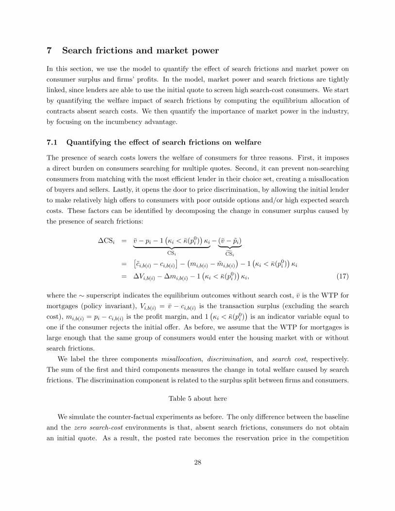
7 Search frictions and market power

In this section, we use the model to quantify the effect of search frictions and market power on

consumer surplus and firms’ profits. In the model, market power and search frictions are tightly

linked, since lenders are able to use the initial quote to screen high search-cost consumers. We start

by quantifying the welfare impact of search frictions by computing the equilibrium allocation of

contracts absent search costs. We then quantify the importance of market power in the industry,

by focusing on the incumbency advantage.

7.1 Quantifying the effect of search frictions on welfare

The presence of search costs lowers the welfare of consumers for three reasons. First, it imposes

a direct burden on consumers searching for multiple quotes. Second, it can prevent non-searching

consumers from matching with the most efficient lender in their choice set, creating a misallocation

of buyers and sellers. Lastly, it opens the door to price discrimination, by allowing the initial lender

to make relatively high offers to consumers with poor outside options and/or high expected search

costs. These factors can be identified by decomposing the change in consumer surplus caused by

the presence of search frictions:

∆CSi = v − pi − 1(κi < κ(p0

i ))κi︸ ︷︷ ︸

CSi

− (v − pi)︸ ︷︷ ︸CSi

=[ci,b(i) − ci,b(i)

]−(mi,b(i) − mi,b(i)

)− 1

(κi < κ(p0

i ))κi

= ∆Vi,b(i) −∆mi,b(i) − 1(κi < κ(p0

i ))κi, (17)

where the ∼ superscript indicates the equilibrium outcomes without search cost, v is the WTP for

mortgages (policy invariant), Vi,b(i) = v − ci,b(i) is the transaction surplus (excluding the search

cost), mi,b(i) = pi − ci,b(i) is the profit margin, and 1(κi < κ(p0

i ))

is an indicator variable equal to

one if the consumer rejects the initial offer. As before, we assume that the WTP for mortgages is

large enough that the same group of consumers would enter the housing market with or without

search frictions.

We label the three components misallocation, discrimination, and search cost, respectively.

The sum of the first and third components measures the change in total welfare caused by search

frictions. The discrimination component is related to the surplus split between firms and consumers.

Table 5 about here

We simulate the counter-factual experiments as before. The only difference between the baseline

and the zero search-cost environments is that, absent search frictions, consumers do not obtain

an initial quote. As a result, the posted rate becomes the reservation price in the competition

28

stage. Table 5 presents the main simulation results. Columns 1 through 3 show the change in the

misallocation, discrimination and search cost components respectively, while column 4 presents the

total change in consumer surplus. To illustrate the heterogeneity across consumers, the first line

reports the fraction of simulated consumers experiencing zero changes, and the next four describe

the conditional distribution of non-zero changes. To calculate the cumulative changes, we average

the changes across all qualifying consumers. The percentage shares of each component are expressed

relative to the cumulative changes.

We estimate that the cumulative reduction in consumer surplus associated with search frictions

is equal to $12.80 per month, or 2% of the total interest cost of mortgages in our data set. The largest

component (50%) is attributed to the sunk cost of searching, followed by the increase in margins

associated with price discrimination (28%), and misallocation (21%). Over 98% of consumers are

affected. The sum of the misallocation and discrimination components corresponds to the effect of

search frictions on monthly payments alone: $6.37/month on average per borrower. This leads to

an increase in interest payments of $503 over 5 years (Column (5)), or $1, 569 for consumers who

are directly impacted by the price change.

The sum of the misallocation and search-cost components corresponds to the total welfare cost

of search frictions: $9.15/month per borrower. For these two components, the fraction of zero

changes measures the percentage of buyers and sellers that are matched efficiently and the fraction

of non-searchers in the presence of search frictions, respectively. Search frictions cause 17% of

transactions to be misallocated, despite the fact that more than 32% of consumers do not search.

Note that the difference between these two fractions would be close to zero if the loyalty advantage

were null. Since banks’ fixed-effects are not highly dispersed, this is mostly because consumers visit

the highest expected surplus seller first, which reduces the fraction of inefficient matches.

Focusing directly on the change in profit margins, Column (2) shows that the relatively small

contribution of the discrimination component is explained by the fact that some consumers pay

higher markups in the frictionless market. The median change in profit margins is equal to $12.43

per month; significantly more than the median increase in search costs (i.e. 12.43 vs 7.86). However,

the 10th percentile consumer benefits from a $7.59 reduction in profit margins, which brings the

cumulative effect down to $3.64.

To understand this heterogeneity, recall that the initial quote is used both as a screening tool,

and as a price ceiling in the competition stage. The home bank is in a monopoly position in the

first stage, and can set individual prices based on consumers’ expected outside options. This is

analogous to first-degree price discrimination, and strictly increases the expected profit of the home

bank. This adverse effect is weighed against the fact that the initial offer can be recalled, and so

protects consumers against excessive market power in the competition stage. In the zero search-cost

environment, the price ceiling is on average higher (i.e. it is the posted-rate), which explains why

some consumers experience an increase in profit margins after eliminating search frictions.

29

To put these numbers in perspective, column (6) summarizes the distribution of consumer-

surplus changes arising from eliminating market power entirely, relative to the zero search-cost

environment. We calculate the difference in surplus between the zero search-cost environment, and

one with no search frictions and zero profits margins. This is equivalent to shifting the bargaining

power entirely to consumers in the competition stage, and therefore maximizing the surplus of con-

sumers. Relative to the baseline environment, eliminating market power and search frictions would

increase consumer surplus by $27.92/month on average (i.e. 12.80+15.12). Therefore, eliminating

search frictions would allow consumers to reach 46% of their maximum surplus.

These results can be compared to those of Gavazza (2016), who performs a similar decomposition

of the effect of search frictions on welfare in decentralized asset markets. Using data from the

business aircraft market, he finds that, relative to his estimated model, when search costs are set

to zero welfare falls slightly (by roughly $1 million per quarter). This small decrease is the result

of a reduction in direct search costs (of about $6 million), a reduction of misallocation ($3 million)

and an offsetting increase in dealer costs ($11 million).

7.2 Quantifying the importance of market power

Figure 1 about here

Overall, we find that the market is competitive. Figure 1a plots the distribution profit margins.

The average profit margins is 22.1 bps, which corresponds to a Lerner index of 3.2%. This is

consistent with our earlier findings that mortgage contracts are fairly homogenous across lenders,

and search-costs represent a small share of consumers’ overall mortgage spending. It is also fairly

consistent with the findings in Allen et al. (2014a), which suggest margins of around 35 bps before

the merger and 40 bps afterwards.

This implies that a large fraction of the observed spread between negotiated rates and the 5-year

bond-rate corresponds to transaction costs. We estimate that each contract costs roughly 100 bps

to originate, beyond the financing cost, which is proxied by the bond rate. This cost stems from

a variety of sources: the compensation of loan officers (bonuses and commissions), the advantage

associated with pre-payment risks, transaction costs associated with the securitization of contracts,

as well as upstream profit margins from financing.

The distribution of profit margins is also very dispersed. The coefficient of dispersion of profit

margins is equal to 72%, and the range exceeds 100 bps. Figure 1b shows that part of this dispersion

is caused by heterogeneous search efforts. On average, firms charge a markup that is 90% larger

on consumers who are not searching (i.e. 32.1 vs. 16.9). The margin distribution for searchers also

exhibits an important mass between 0 and 20 bps, and the median margin among searchers is only

13 bps (compared to 32 bps in the non-searcher sample).

The dispersion in profit margins also reflects the fact that market-power arises from a variety

of sources: (i) price discrimination, (ii) loyalty advantage, (iii) observed cost differences (i.e. bank

30

fixed effects and network size), and (iv) idiosyncratic cost differences (i.e. ωij).

The last two components ensure positive profits margins in the competition stage. On av-

erage, the difference between the lowest and second-lowest cost among rival lenders is equal to

$15.70/month. This is the profit margin that would be realized if the home bank were not present

and there were no posted-rate (i.e. ceiling), and therefore can be thought of as an upper bound

on the market power of rival banks. In practice, rival lenders earn slightly less: banks’ average

profits from switching consumers are $14.99/month (or 17.1 bps), compared to $20.22/month for

loyal consumers (or 24.6 bps).

The profit gain from loyalty corresponds to an incumbency advantage: Banks with a large

consumer base have more market power because of a first-mover advantage and loyalty advantage

(or differentiation). We find that the loyalty advantage is substantial: the average home-bank cost

advantage is 33% larger than the standard-deviation of idiosyncratic cost differences. As a result

the home bank is able to retain, on average, 51% of searching consumers. The first-mover advantage

arises because the home bank is in a quasi-monopoly position in the first-stage of the game, and can

price discriminate between consumers based on heterogeneity in their expected reservation prices.

The ability to make the first quote allows the home bank to charge a higher markup and retain a

larger fraction of consumers who, absent search costs, would choose another lender.

To measure the source and magnitude of the incumbency advantage, we use the simulated model

to evaluate the correlation between the size of a lender’s consumer base and its profitability. In the

model, the consumer base of a given bank is defined as the share of consumers with whom it has an

existing day-to-day banking relationship, and this base determines the fraction of consumers in a

given market who start their search with the bank (i.e. ψij). Recall that this matching probability

is defined at the level of a neighborhood (FSA), income group, and year. We use this definition

to construct markets that each have a homogenous consumer base distribution, and we construct

measures of profits and concentration at this level of aggregation. Doing so yields slightly more

than 8, 000 unique markets.

To construct a measure of consumer base that is comparable across markets, we compute,

for each market i, the ratio of the matching probability of lender j over the average matching

probability among banks in the market:

Matching probability ratio =ψij

ψi=

ψijni + 1

.

Table 6 about here

Table 6a summarizes the distribution of contracts and profits across different types of lenders.

The table ranks banks from the smallest consumer base (i.e. between 0 and 25% of the average

size in the same market), to the largest (i.e. between 4 and 7 times the average size). As we saw

earlier, most consumers choose a mortgage lender with a large branch presence. This is reflected

31

in the distribution of contracts shown in column (1): 46% of contracts are issued by banks with a

consumer base between 1 and 2 times larger than the average bank in their market.

Columns (2) and (3) report the weighted average share of profits and contracts generated by

each bank type. To get this number, for each market, we calculate the average share of profits

and contracts generated by lenders with consumer bases belonging to one of the 6 categories. We

then aggregate these shares across markets, using the total number of contracts originated in each

market as weight.

If there were no relationship between banks’ consumer bases and mortgages, contracts and

profits would be uniformly distributed across categories (i.e. would be about 12% on average).

The resulting distributions are significantly more concentrated. Banks in the top category (4 to 7)

earn, on average, 62% of the profits generated in their respective markets, compared to only 2%,

on average, for the smallest banks. Note that the average profit share increases very quickly with

the size of the consumer base.

In addition, the distribution of profits is more concentrated than the distribution of contracts.

On average the top lenders originate 54% of contracts, but earn 62% of the profits. This pattern

reflects the fact that banks with a large consumer base charge, on average, higher markups. Column

(5) shows that the average profit margin for banks in the top category is equal to 30.7 bps, compared

to only 16.6 bps for banks in the bottom category. This discrepancy is largely explained by the

difference in markups between searchers and non-searchers. Banks in the smallest consumer-base

category earn on average 90% of their profits from consumers reaching the second stage of the

game, compared to 40% for banks in the largest category. This confirms the importance of the

first-mover advantage as a source of market power for large consumer base lenders.

Identifying the relative importance of the first mover advantage and differentiation is not an

easy task however, since the two interact to generate a correlation between profitability and size

of consumer base. For instance, the profit gain from being able to make the first offer depends on

the amount of differentiation, since lower-cost banks have more leverage in the initial negotiation

stage. Similarly, the presence of a cost advantage reduces the incentive for consumers to search,

and increases the fraction of profits generated from price discrimination.

To measure each of the components that generate the incumbency advantage, we simulate a

series of counter-factual experiments aimed at varying the first-mover advantage and the differen-

tiation component independently. In particular, to eliminate the differentiation component, CF-1

simulates a model in which the cost-advantage of the home bank is set to zero, which is analogous to

separating the provision of mortgages from other banking services. We eliminate the ability of firms

to screen high search-cost consumers by imposing a uniform matching probability and breaking the

link between the ability to make the first offer and the size of the consumer base (CF-2). Finally,

CF-3 combines the previous two environments by assuming a uniform matching probability and

32

zero loyalty advantage.28

Results are displayed in Table 6b. The top panel summarizes concentration in the industry, as

well as the dispersion in profit margins between large and small banks. The bottom panel describes

some of the key equilibrium outcomes in the baseline and counter-factual environments. The ratio

of the profit margin of large and small banks is a measure of the incumbency advantage: how

much more market power do banks with large consumer bases have relative to banks with small

consumer bases. In the baseline environment, we estimate that large banks’ profit margins are

85.1% larger. Eliminating the first-mover and the loyalty advantage shrinks the margin difference

to 14.5% (CF-3), and so this is a measure of the market power of large banks that stem solely from

brand and branch network differences.29 The difference, or 0.707 = 1.851− 1.145, is explained by

the incumbency advantage.

The first column of Table 6c summarizes the incumbency advantage in terms of profit margins,

profit shares, and market shares (or contract). Columns (2) to (4) use the uniform matching

probability (CF-2) and the zero loyal advantage (CF-1) counter-factual environments to decompose

the incumbency advantage into three terms:

Incumbency advantange︸ ︷︷ ︸0.707

= Loyalty advantage︸ ︷︷ ︸0.34

+ Price discrimination︸ ︷︷ ︸0.22

+ Interaction︸ ︷︷ ︸0.14

.

Therefore, relative to CF-3, almost 50% of the market-power of large banks is caused by the

home-bank cost advantage, just over 30% by the first-mover advantage, and the remaining 20% is

explained by the interaction of both elements.

The interaction term originates from the joint equilibrium effect of differentiation and the order

of moves on the search probability. As the middle panel indicates, the combined effect of the

home-bank cost and first-mover advantage is to lower the search probability from 82.2% to 65.6%,

which increases the profit margin ratio by an extra 14 percentage points through a change in the

composition of loyal borrowers. Independently, the two elements have little or no effect on the

search probability relative to the CF-3 environment.

The concentration of profits and contracts is similarly impacted. Eliminating both the loyalty

advantage and the first-mover advantage substantially reduces the concentration of profits: large

banks’ share of profits is 35.72 times larger than that of small banks in the baseline, compared

to only 6.70 times in CF-3. As with margins, the loyalty advantage alone explains a bigger share

of the drop in concentration (36%) than the first-mover advantage (17%). However, unlike with

margins, a larger portion of the profit share ratio is explained by the interaction of differentiation

28An alternative approach for eliminating the first-mover advantage is to set consumer search costs to zero. Wechose instead to modify the order of moves by setting ψij = 1/(n+ 1), since doing so does not fundamentally changethe degree of competition in the market. The zero search-cost counterfactual yields very similar conclusions. Resultsare available from the authors upon request.

29All ratios would be equal to one if the difference between lenders were caused only by idiosyncratic cost differences.

33

and discrimination: 47% of the profit share difference between large and small banks is explained

by the interaction term. This is because the increase in the search probability from letting the

most efficient lender make the first offer has a very large effect on banks’ retention probability, and

therefore on their overall profitability.

8 Conclusion

The paper makes three main contributions. The first is to provide an empirical framework for

studying markets with negotiated prices. The second is to show that search frictions are important

and generate significant welfare losses for consumers that can be decomposed into misallocation,

price discrimination, and direct search cost components. Finally, the paper also demonstrates the

importance of having a large consumer base for market power, and decomposes the effect into a

first-mover advantage and brand loyalty. We find that brand loyalty is the most important source

of market power, but search frictions play an important role through the first-mover advantage.

A few caveats should be mentioned. First, the assumption that monthly payment has no effect

on the loan size could imply (depending on the elasticity of loan demand) that the distortions

arising from search and market power are larger than the ones we calculate. Second, although the

overall fit of our model is good, it predicts that loyal consumers pay more than they are observed

to in the data. This difference is directly related to our modeling assumptions: the timing and

order of search are the same for all consumers, and all consumers have a single home bank. These

are simplifying assumptions that closely link search and switching in the model.

The model also over-estimates the impact of competition on rates, likely because market struc-

ture is assumed to be independent of consumers’ unobserved attributes, up to regional fixed-effects.

Otherwise, our estimates of firms’ cost differences would suffer from an attenuation bias, and our

results would correspond to a lower bound on margins. A related interpretation of the small

reduced-form effect of competition on rates is that consumers face heterogenous consideration sets,

conditional on being located in the same area. This would create measurement error in consumer

choice sets, which is computationally prohibitive to incorporate, since lenders are ex-ante hetero-

geneous. Moreover, we do not have data on the set, or identity, of lenders considered by borrowers.

References

Alexandrov, A. and S. Koulayev (2017, April). No shopping in the U.S. mortgage market: Directand strategic effects of providing information. working paper, CFPB No. 2017-01.

Allen, J., R. Clark, and J. F. Houde (2014a). The effect of mergers in search markets: Evidencefrom the Canadian mortgage industry. American Economic Review 104, 3365–3396.

Allen, J., R. Clark, and J. F. Houde (2014b). Price dispersion in mortgage markets. Journal ofIndustrial Economics 62, 377–416.

34

Beckert, W., H. Smith, and Y. Takahashi (2016). Competition and price discrimination in aspatially differentiated product market with negotiated prices. Working paper, John HopkinsUniversity.

Bester, H. (1988). Bargaining, search costs and equilibrium price distributions. Review of Eco-nomic Studies 55 (1), 201–214.

Brannan, L. and L. M. Froeb (2000, May). Mergers, cartels, set-asides, and bidding preferencesin asymmetric oral auctions. The Review of Economic and Statistics 82 (2), 283–290.

Bronnenberg, B. J. and J. Dube (2017). The formation of consumer brand preferences. AnnualReview of Economics 9, 353–382.

Busse, M., J. Silva-Risso, and F. Zettelmeyer (2006). $1,000 cash back: The pass-through of automanufacturer promotions. American Economic Review 96 (4).

Chatterjee, K. and C. C. Lee (1998). Bargaining and search with incomplete information aboutoutside options. Games and Economic Bahavior 22, 203–237.

Cicala, S. (2015). When does regulation distort costs? Lessons from fuel procurement in USelectricity generation. American Economic Review 105, 411–444.

Crawford, G. and A. Yurukoglu (2012). The welfare effects of bundling in multichannel television.American Economic Review 102 (2), 643–685.

Dafny, L. (2010). Are health insurance markets competitive? American Economic Review 100 (4),1399–1431.

De Los Santos, B., A. Hortacsu, and M. Wildenbeest (2012). Testing models of consumer searchusing data on web browsing and purchasing behavior. American Economic Review 102, 2955–2980.

Dell’Ariccia, G., E. Friedman, and R. Marquez (1999). Adverse selection as a barrier to entry inthe banking industry. RAND Journal of Economics 30, 515–534.

Doornik, J. A. (2007). Ox - An Object-Oriented Matrix Programming Language. TimberlakeConsultants Press and Oxford.

Duffie, D., N. Garleanu, and L. H. Pedersen (2005). Over-the-counter markets. Economet-rica 73 (6), 1815–1847.

French, E. and C. Taber (2011). Identification of Models of the Labor Market, Chapter 6. Hand-book of Labor Economics. Elsevier B.V.

Fudenberg, D. and M. Villas-Boas (2007). Behavior-based price discrimination and customerrecognition. In Economics and Information Systems, Volume 1. Oxford: Elsevier Science.

Gavazza, A. (2016). An empirical equilibrium model of a decentralized asset market. ForthcomingEconometrica.

Goldberg, P. K. (1996). Dealer price discrimination in new car purchases: Evidence from theconsumer expenditure survey. Journal of Political Economy 104 (3), 622–654.

Gowrisankaran, G., A. Nevo, and R. Town (2015). Mergers when prices are negotiated: Evidencefrom the hospital industry. American Economic Review 105, 172–203.

Grennan, M. (2013). Price discrimination and bargaining: Empirical evidence from medicaldevices. American Economic Review 103 (1), 145–177.

35

Hall, R. E. and S. Woodward (2012, December). Diagnosing consumer confusion and sub-optimalshopping effort: Theory and mortgage-market evidence. American economic Review 102 (6).

Ho, K. and R. Lee (2017). Insurer competition in health care markets. Econometrica 85, 379–417.

Hong, H. and M. Shum (2006). Using price distributions to estimate search costs. RAND Journalof Economics 37 (2), 257–275.

Honka, E. (2014). Quantifying search and switching costs in the u.s. auto insurance industry.RAND Journal of Economics 45, 847–884.

Honka, E., A. Hortacsu, and M. A. Vitorino (2017). Advertising, consumer awareness, and choice:Evidence from the U.S. banking industry. Rand Journal of Economics 48, 611–646.

Horn, H. and A. Wolinsky (1988). Bilateral monopolies and incentives for merger. The RANDJournal of Economics 19 (3), 408–419.

Hortacsu, A. and C. Syverson (2004). Product differentiation, search costs, and competitionin the mututal fund industry: A case study of S&P 500 index funds. Quarterly Journal ofEconomics, 403–456.

Imbens, G. and T. Lancaster (1994, October). Combining micro and macro data in microecono-metric models. The Review of Economic Studies 61 (4), 655–680.

Jindal, P. and P. Newberry (2017). To bargain or not to bargain: The role of fixed costs in pricenegotiations.

Joskow, P. L. (1987). Contract duration and relationship-specific investments: The case of coal.American economic Review 77, 168–185.

Lewis, M. and K. Pflum (2015, February). Diagnosing hospital system bargaining power inmanaged care networks. American Economic Journal: Economic Policy 7 (1), 243–74.

Marshall, G. (2016). Search and wholesale price discrimination. Working paper, University ofIllinois.

Petriconi, S. (2015). Bank competition, information choice and inefficient lending booms. Work-ing paper.

Postel-Vinay, F. and J.-M. Robin (2002). Equilibrium wage dispersion with worker and employerheterogeneity. Econometrica 70 (2), 2295–2350.

Ridder, G. and R. Moffitt (2007). The econometrics of data combination. In Handbook of Econo-metrics, pp. 5469–5547.

Salz, T. (2015). Intermediation and competition in search markets: An empirical case study.working paper, NYU.

Scott-Morton, F., F. Zettelmeyer, and J. Silva-Risso (2001). Internet car retailing. Journal ofIndustrial Economics 49 (4), 501–519.

Sorensen, A. (2001, October). An empirical model of heterogeneous consumer search for retailprescription drugs. Working Paper 8548, NBER.

Town, R. and G. Vistnes (2001). Competition in networks: An analysis of hospital pricingbehavior. Journal of Health Economics 20, 719–753.

Van den Berg, G. and B. van der Klaauw (2001). Combining micro and macro unemploymentduration data. Journal of Econometrics 102, 271–309.

36

White, H. (1982). Maximum likelihood estimation of misspecified models. Econometrica 50, 1–25.

Wildenbeest, M. R. (2011). An empirical model of search with vertically differentiated products.RAND Journal of Economics 42 (4), 729–757.

Wolinsky, A. (1987). Matching, search, and bargaining. Journal of Economic Theory 42, 311–333.

37

Table 1: Descriptive statistics on mortgage contracts and loyalty in the selected sample

(a) Summary statistics

(1) (2) (3) (4) (5)VARIABLES Mean Std-dev. P25 P50 P75Interest rate spread 120 59.3 81 115 161Positive discounts 95.3 45.4 70 95 1251(Discount=0) .127 .333 0 0 0Monthly payment 925 385 619 858 1169Total loan ($/100K) 136 57.6 90.4 126 174Income ($/100K) 68.4 27.9 48.5 64.1 82.1FICO score 669 74 650 700 750LTV 91 4.38 89.7 90 951(LTV=Max) .385 .487 0 0 11(Previous owner) .251 .433 0 0 11(Loyal) .737 .440 0 1 1Number of Lenders 8.65 1.44 8 9 10Branch network 1.6 1.02 .989 1.37 1.93

(b) Reduced-form regression

(1) (2)VARIABLES Rate 1(Loyal)1(Loyal) 0.097a

(0.0079)Previous owner 0.025a 0.11a

(0.0084) (0.0072)Branch network 0.023a 0.026a

(0.0046) (0.0045)# Lenders (log) -0.13a -0.076a

(0.022) (0.019)

Observations 20,619 20,619R-squared 0.612 0.095Marg. effect: income 0.29 0.18Marg. effect: loan 0.47 -0.19

Sample size = 26,218. Number of missing loyal observations = 5,599. The sample covers the period from Jan1999 to Oct 2002. We trim the top and bottom 0.5% of observations in terms of income and loan size. Interest ratesand discounts are expressed in percentage basis points (bps). The number of lenders is within 10KM of the borrowersnew home (neighborhood). Relative branch is defined as the average network size of the chosen institution relative tothe average size of others present in the same neighborhood. Each regression also includes market and quarter/yearfixed-effects, and other financial characteristics (i.e. posted-rate, bond-rate, FICO score, LTV, 1(LTV Max), loansize, income, loan/income.). Robust standard errors in parenthesis. Significance levels: a p<0.01, b p<0.05, c p<0.1.

38

Table 2: Maximum likelihood estimation results

Specification 1 Specification 2 Specification 3Baseline

Estimate (S.E.) Estimate (S.E.) Estimate (S.E.)Heterogeneity and preferences

Common shock (σc) 0.356 (0.003) 0.358 (0.003) 0.358 (0.003)Idiosyncratic shock (σω) 0.047 (0.002) 0.102 (0.002) 0.094 (0.002)Avg. search cost (log)α0 -1.539 (0.042) -1.506 (0.026) -1.592 (0.034)αinc 0.458 (0.052) 0.401 (0.038) 0.356 (0.045)αowner 0.184 (0.054) 0.086 (0.059) 0.143 (0.059)

Home-bank WTPλ0 0.064 (0.003) 0.010 (0.007)λowner 0.032 (0.002) -0.016 (0.008)λinc 0.002 (0.003) 0.023 (0.01)

Home-bank cost advantage∆0 0.146 (0.005) 0.126 (0.008)∆owner 0.066 (0.004) 0.075 (0.008)∆inc 0.012 (0.006) -0.010 (0.01)

Cost functionIntercept 5.332 (0.229) 5.495 (0.229) 5.479 (0.23)Bond rate 0.307 (0.026) 0.306 (0.026) 0.306 (0.026)Range posted-rate -0.147 (0.017) -0.145 (0.017) -0.145 (0.017)Total loan -0.220 (0.073) -0.208 (0.073) -0.208 (0.073)Income -0.228 (0.026) -0.214 (0.026) -0.228 (0.027)Loan/Income -0.100 (0.01) -0.102 (0.01) -0.102 (0.01)Previous owner -0.003 (0.007) 0.047 (0.007) 0.051 (0.008)House price 0.222 (0.066) 0.211 (0.066) 0.211 (0.066)FICO -0.662 (0.038) -0.656 (0.038) -0.660 (0.038)LTV 1.111 (0.157) 1.092 (0.158) 1.093 (0.157)1(LTV = 95%) 0.029 (0.008) 0.029 (0.008) 0.029 (0.008)Rel. network size -0.019 (0.001) -0.039 (0.002) -0.036 (0.002)

Range of Bank FE [ -0.041 , 0.038 ] [ -0.088 , 0.063 ] [ -0.08 , 0.059 ]Quarter-year FE Y Y YRegion FE Y Y YSample size 26,218 26,218 26,218LLF/N -2.059 -2.048 -2.047Search moments weight 1 1 1Likelihood ratio test (χ2(3)) 660.678 45.660

Units: $/100 per month. Average search cost function: logα(z1i ) = α0 + αinc log(Incomei) +αownerPrevious owneri. Home-bank willingness-to-pay: λ(z2i ) = Li × (λ0 + λincIncomei + λownerPrevious owneri).Home-bank cost advantage: ∆(z2i ) = Li × (∆0 + ∆incIncomei + ∆ownerPrevious owneri). Cost function: cij =Li × (ci + ωij), where ci ∼ N(xiβ, σ

2c ) and ωij ∼ T1EV

(ξj + ξbranchRel. network sizeij − eσω, σω

). The likelihood-

ratio test compares Models 1 and 2 against Model 3 (alternative hypothesis). The 1% significance level critical valueis 16.266. Specification 2 is our baseline model. Robust standard errors in parenthesis (White 1982).

39

Table 3: Summary statistics on the home-bank cost advantage, search and interest costs.

(a) Home-bank cost advantage

VARIABLES Mean SD P25 P50 P75NHB

Inc.< 60K 15.1 .111 15.1 15.1 15.2Inc.≥ 60K 15.6 .273 15.4 15.5 15.7

POInc.< 60K 21.7 .107 21.6 21.7 21.8Inc.≥ 60K 22.3 .336 22 22.2 22.4

(b) Search and interest cost

VARIABLES Mean SD P25 P50 P75NS Total SC 2.3 1.3 1.47 2 2.82

Interest cost 44.2 18.3 30.1 40.9 55.3S Total SC .549 .443 .203 .461 .809

Interest cost 45.6 19 30.6 42.6 57.6Total Total SC 1.15 1.19 .323 .784 1.58

Interest cost 45.1 18.8 30.4 42 56.9

Acronyms: NHB = New home buyers; PO = Previous owners; NS = Non searchers; S = Searchers; Total SC =Total search cost. Units Table 3a: $/Month. The cost advantage is measured for a $100, 000 loan. Units Table 3b:$/1,000. The search and interest costs correspond to the total over the term of the mortgage contract (60 months).

40

Table 4: Summary statistics for simulated and observed data

(a) Negotiated price and bank choice

Spread Discounts 1(Discount=0) Payment 1(Loyal) Network size(bps) (bps) ($/Month) (relative)

Observed:Mean 119.5 95.3 0.127 924.6 0.651 1.599SD 59.3 45.4 0.333 385.0 0.477 1.015

Simulated:Mean 119.4 92.2 0.092 962.8 0.670 1.678SD 62.0 53.4 0.289 397.3 0.470 1.136

(b) Search probabilities

Baseline Zero moment Large moment Survey data(ρ = 1) weight (ρ = 0) weight (ρ = 100) Freq. Mg

Cit

y Pop. > 1M 0.673 0.717b 0.661 0.660 3381M > Pop. > 100K 0.657 0.695 0.639 0.654 268Pop. ≤ 100K 0.628b 0.655a 0.584 0.560 275

Reg

ion

s East 0.626a 0.656a 0.582 0.557 289West 0.651 0.688c 0.628 0.643 327Ontario 0.673 0.713 0.659 0.668 265

Inc. > $60K 0.639a 0.670a 0.586 0.579 400

≤ $60K 0.669 0.712b 0.670 0.666 441Total 0.657c 0.694a 0.635 0.625 841

The simulated sample is obtained by simulating 300,000 contracts from the baseline model, and dropping con-sumers who fail to qualify for a loan (5.5%). Spread is defined as transaction rate minus bond rate.

41

Table 5: Decomposing the effect of search frictions on welfare

Consumer surplus change: Zero search-cost Change Change: CSMisc. Disc. Search Total Interest Market-

($/M.) ($/M.) ($/M.) ($/M.) Cost ($) Power ($/M.)(1) (2) (3) (4) (5) (6)

Zero changes % 0.83 0.68 0.32 0.02 0.68 0.00Distribution: Non-zero changes

Mean -16.32 11.37 9.49 -13.03 1569 -15.12P10 -33.44 -7.59 1.46 -26.55 344 -34.24P50 -11.70 12.43 7.86 -10.56 1591 -9.89P90 -2.19 28.48 19.01 -1.68 2697 -1.53

Cumulative $ -2.73 3.64 6.42 -12.80 503 -15.12% 0.21 0.28 0.50 1.00

Each entry corresponds to an average over 300,000 simulated contracts. Statistics in lines 2-5 are calculatedusing the samples of consumers facing non-zero changes. Cumulative changes are the sum of all changes divided bythe total number of qualifying consumers. The welfare decomposition in columns (1)-(3) corresponds to: ∆CSi =∆Vi − ∆mi − ∆κiSi. The last row reports the contribution of each component, in %, to the cumulative change.Column (5) summarizes the effect of search frictions on the total interest payment over 5 years: Total interest cost(κi > 0) - Total interest cost (κi = 0). The last column reports the further reduction in consumer surplus arisingfrom the presence of market power in the second-stage of the game: CS(κi = 0,mi > 0)− CS(κi = 0,mi = 0).

42

Table 6: Incumbent advantage and market power

(a) Distribution of bank profitability and consumer base in the baseline environment

Consumer Matching Sample Within market shares Second stage Marginsbase probability frequency Profits Contracts profits (%) (bps)

ratio (1) (2) (3) (4) (5)Small 0 to 1/4 0.05 0.02 0.02 0.90 16.6

1/4 to 1/2 0.04 0.04 0.05 0.62 19.11/2 to 1 0.17 0.07 0.08 0.51 18.91 to 2 0.46 0.16 0.16 0.50 20.42 to 4 0.25 0.34 0.30 0.51 24.0

Large 4 to 7 0.04 0.62 0.54 0.40 30.7

(b) Distribution of bank profitability in the baseline and counterfactual environments

Statistics Variables Baseline CF-1 CF-2 CF-3∆i = 0 ψi = 1/(n+ 1) ψi = 1/(n+ 1) & ∆i = 0

Ratio: Large base/Small baseMargins (bps) 1.851 1.369 1.485 1.145Profit shares 35.717 11.652 17.159 6.699Contract shares 24.582 9.769 13.204 6.243

Full sample averagesSearch probability 0.656 0.774 0.838 0.8222nd stage profits (%) 0.531 0.727 0.809 0.784Margins (bps) 22.07 18.56 21.34 18.60Match prob. ratio 1.709 1.546 1.605 1.439

(c) Decomposition of the incumbency advantage

Large/Small Incumbency adv. Loyalty premium Price discrimination InteractionRatio Base − CF-3 CF-2− CF-3 CF-1− CF-3Margins 0.707 0.340 0.224 0.142

(0.48) (0.32) (0.2)Profit share 29.018 10.460 4.954 13.605

(0.36) (0.17) (0.47)Contract share 18.339 6.961 3.526 7.852

(0.38) (0.19) (0.43)

Each entry in Table 6a is the weighted average outcome of lenders belonging to each category (rows). Theweights are proportional to the number of contracts originated in each market (i.e. neighborhood/year/income).Variable definitions: Matching probability ratio = Consumer base of bank j / Average consumer base; Sample fre-quency = Market share of lenders in each category; Second-stage profit (%) = Average share of profits originatingfrom the searching consumers; Within market share = Average share of profits or contracts generated by lenders ineach category; Margins in percentage basis points; Ratio: Large base/Small base = Ratio of the average outcomesof lenders in the large group, over those in the small group. Counter-factual environments: (1) Zero home-bank costadvantage, (2) Uniform matching probability, (3) combination of (1) and (2).

43

Figure 1: Distribution of profit margins

(a) Full sample

0.0

5.1

.15

.2.2

5Fr

eque

ncie

s

0 10 20 30 40 50 60 70 80 90 100+Average = 22.1, Std-Deviation = 16

Profit Margins (bps)

(b) Searchers and non-searchers

0.1

.2.3

.4Fr

eque

ncie

s

0 10 20 30 40 50 60 70 80 90 100+Searchers: avg. = 16.9, std-dev. = 14.6 / Non-Searchers: avg. = 32, std-dev. = 14.

Profit Margins (bps)

Non-searchersSearchers

44