Screening Equilibria In Experimental Markets Lisa L. …aria.org/rts/proceedings/1999/posey_99.pdf2...

Screening Equilibria In Experimental Markets

Lisa L. Posey ([email protected])Abdullah Yavas ([email protected])

Penn State University409 Business Administration Building

University Park, PA 16802

January 1, 1999

1On the twentieth anniversary of the paper’s publication, the European Group of Risk andInsurance Economists held a conference honoring this classic article. The conference featuredMichael Rothchild, Joseph Stiglitz and others presenting papers inspired by the original workwhich were subsequently published in a special edition of the Geneva Papers on Risk andInsurance Theory (1997).

1

1. Introduction

In their classic paper, Rothschild and Stiglitz (1976) analyze a competitive insurance

market under asymmetric information with two policyholder risk types, or probabilities of having

a fixed loss amount. Their model is a screening model where uninformed insurers move first

offering a menu of contracts, defined as price-quantity pairs, to informed policyholders. They

conclude that the only Nash equilibrium in this setting is a separating equilibrium, and that this

equilibrium exists only if the proportion of high risk policyholders is sufficiently large. In this

equilibrium the price-quantity pairs allow insurers to deduce policyholder risk types by their

contract choices.

This paper by Rothschild and Stiglitz has spurred on a tremendous amount of additional

research. This subsequent research is noteworthy in terms of the wide variety of fields to which

the model has been applied. In addition to inspiring papers which directly apply the Rothschild-

Stiglitz model, the paper has been cited several hundred times in the twenty-one years since its

publication.1

One body of research which followed the paper’s publication sought to develop

alternative equilibrium concepts to be applied to the same type of problem studied by Rothschild

and Stiglitz, the competitive insurance market with asymmetric information. These include most

notably Wilson (1977), and Riley (1979). Wilson’s equilibrium concept allowed for behavior by

insurers called “Wilson foresight”. Miyazaki (1977) and Spence (1978) established that under

2

this new type of behavior an equilibrium always exists. It is either the Rothschild-Stiglitz

equilibrium or a pooling equilibrium. Riley presented a model with “reactive” firms which

always sustains an equilibrium. Both the Miyazaki-Wilson and Riley equilibria are non-Nash

equilibria.

Another body of research has extended the Rothschild-Stiglitz model to analyze insurance

markets with asymmetric information more extensively. This research includes studies on the

efficiency implications of the Rothschild-Stiglitz model when compared to Miyazaki-Wilson and

Riley (Crocker and Snow, 1985), studies of the efficiency of the use of categorical discrimination

in insurance markets (Crocker and Snow, 1986; Hoy, 1982) and studies of the social value of

hidden information (Crocker and Snow, 1992; Doherty and Thistle, 1996; and Doherty and

Posey, 1998). It has also been used to study multi-period insurance contracts (Cooper and Hayes,

1987; Hosios and Peters, 1989), and has been extended to include uncertainty about the size of

losses (Doherty and Schlesinger, 1995) and policyholder uncertainty about risk type (Ligon and

Thistle, 1996). Numerous other issues in insurance markets have been analyzed with the

Rothschild-Stiglitz model from supply restrictions in liability insurance markets (Berger and

Cummins, 1992) to the financing of charitable hospital care (Posey, 1997).

This screening model of adverse selection has been applied to issues in many fields other

than insurance. It has been applied to credit markets (Stiglitz and Weiss, 1992) including

mortgage lending (Brueckner, 1992, 1994; Chari and Jagannathan, 1989; LeRoy, 1996) and

lending to entrepreneurs (De Maza and Webb, 1990). In the law and economics literature, the

model has been applied to attorney fee structures (Rubinfeld and Schtchmer, 1993) and in the

conflict resolution literature it has been applied to arbitration (Curry and Pecorino, 1993).

2 Berg, Dickhaut and Senkow (1987) focus on discriminating between the Rothschild-Stiglitz, Wilson and Riley models which is not a focus of our experiments.

3

Unemployment has been proposed as a screening device for worker productivity (Stiglitz,

Rodriguez and Nalebuff , 1993). The wide variety of other applications is numerous.

Given the widespread application of this model in so many fields, empirical investigation

would be particularly valuable. The empirical tests which focus on automobile insurance markets

have provided mixed results. D’Arcy and Doherty (1990) and Dionne, Gourieroux and Vanasse

(1998) have not found support for the Rothschild-Stiglitz adverse selection model in automobile

insurance markets in the United States or Canada, while Dahbly (1983) and Puelz (1990) have

found support. In the medical insurance and life insurance markets, the model is supported by the

empirical evidence (Beliveau, 1981; Browne and Doerpinghaus (1993); Browne, 1992).

In this paper, we conduct an experimental test of the Rothschild-Stiglitz screening model

of insurance markets with asymmetric information. Our focus is on the strategic behavior of

firms with the option to offer menus of contracts to screen policyholders by risk type. Although a

number of experiments have tested separating versus pooling equilibria in signaling models (e.g.,

Miller and Plott, 1985; Cadsby, Frank and Maksimovic, 1990), we have found only one other

experimental test of a screening model (Berg, Dickhaut and Senkow, 1987). In that paper, to

make the procedure more tractable for the subjects, the designers of the experiment limited the

choice of sellers to four contracts (price-quantity pairs). This very strong restriction is necessary

because of the complexity of the model. 2 In our experiment, we allow sellers to offer one or both

of two quantities of insurance, full coverage or partial coverage, and effectively allow them to

choose any price above zero in increments of .10 units. To make the procedure more tractable for

4

participants in our experiment, the buying decisions are made by a computer and we focus on the

behavior of sellers and whether they indeed attempt to screen buyers by risk type in an

environment where sellers have many contract options.

We develop a parameterized example of the Rothschild-Stiglitz screening model and

utilize these parameters to design our experimental sessions. Our results provide striking

evidence for screening behavior by sellers. We first conduct three sessions of our experiment in

which the proportion of high risks is such that a Rothschild-Stiglitz separating equilibrium

should exist. Each session involves 30 rounds, and in each round sellers compete for potential

policyholders of two types, high and low risk. In each of these sessions, by the final round 100%

of the markets have the Rothschild-Stiglitz separating equilibrium outcome, and 98.3% of

markets have the Rothschild-Stiglitz separating equilibrium in the last 10 rounds. Not only are

sellers in our experiment able to screen high risk and low risk buyers, they also price both full

coverage and partial coverage contracts at their equilibrium levels. We then conduct three more

sessions in which the only change we make is decreasing the proportion of high risks such that

the Nash equilibrium is now a pooling equilibrium where the sellers offer only the full coverage

contract. Once again, the observed behavior converges to the equilibrium prediction, although at

a slower rate than it did in the three separating equilibrium sessions. In all but one of the last 10

rounds of each session, the observed outcome is a pooling outcome where only the full coverage

contract is offered. However, there are some deviations from the equilibrium pricing.

Approximately 13% of the full coverage contracts are sold at a price other than the equilibrium

price (usually one increment above or one increment below).

Given the complexity of the Rothschild-Stiglitz model and the complexity of the resulting

5

experimental design, the fact that the theory performed so well in our experiments is somewhat

surprising. We believe the explanation lies in the simplicity of the competition involved in the

model, the Bertrand type price competition. A price cut by one seller would capture the whole

market for that seller. As a result, the other sellers have to match that price cut, otherwise they

would not be able to sell any units. In our separating sessions, the price competition quickly

results in both partial coverage and full coverage contracts being offered at their equilibrium

prices. The convergence to the equilibrium in the pooling sessions is slower because it essentially

involves two steps. In the first step, some sellers have to realize that instead of offering both

contracts they could steal all the high risk and low risk buyers by offering the full coverage

contract only. Realizing that they are losing their customers to a pooling contract, other sellers

follow. Once all the sellers begin to offer the full coverage pooling contract, price competition

eventually forces the price of the full coverage contract to its equilibrium level.

The next section presents the Rothschild and Stiglitz model and a parameterized example

of it. These parameters are utilized in our experiment. Section 3 describes the design of the

experiment. Experimental procedures are provided in Section 4. Section 5 reports the results of

the experiment. Section 6 offers concluding remarks.

2. Rothschild-Stiglitz Model

Rothschild and Stiglitz (1977) develop a model of a competitive insurance market with

asymmetric information. All potential policyholders are endowed with initial wealth W and each

faces two possible states of nature, the loss state, with a reduction in wealth to W-X, and the no

loss state where wealth remains at W. They assume two types of potential policyholders (or

6

customers), high risk and low risk. The probability of the loss state is pL for low risks and pH for

high risks, with pL < pH. The corresponding probability of the no loss state for type i is1- pi,

i=L,H . The proportion of high risk individuals in the market is � and 1- � is the proportion of low

risk individuals. All parties know W, �, pL, pH, X and the utility function of potential

policyholders U(·) defined over wealth. But each customer’s probability of a loss is private

information to that customer and the insurers know only the proportion of high and low risks, not

which customers are which risk type. Potential policyholders are expected utility maximizers and

it is assumed that U' >0 and U''<0.

Rothchild-Stiglitz Equilibrium

The type of equilibrium considered by Rothchild and Stiglitz is a Nash equilibrium. The

insurance premium paid in all states of nature is . and I is the payment made to the insured in the

loss state. Therefore, an insurance contract can be defined as a pair (., I). An equilibrium is

defined as a set of contracts such that, when each customer chooses a contract to maximize his or

her expected utility, no equilibrium contract yields negative profits and no insurer has an

incentive to offer contracts outside the equilibrium set. The Rothschild-Stiglitz equilibrium is a

screening equilibrium which induces individuals of each risk type to buy the policy or contract

designed for them and, consequently, reveal their information. Let (.i, Ii) represent a contract

intended for a type i individual, i=L,H . The equilibrium consists of a low risk and high risk

contract solving the following maximization problem:

Max (1-pL)U(W-.L)+pLU(W-X-.L+I L) (1)

subject to (1-pH) U(W-.H)+pHU(W-X-.H+I H)

7

-(1-pH)U(W-.L)-pHU(W-X-.L+I L)=0 (2)

.H-pHIH=0 (3)

and .L-pLIL=0. (4)

The solution gives low risks the highest utility possible while ensuring that high risks do not

choose the low risk policy, due to the self-selection constraint (2) and that the low and high risk

policies each break even, or are actuarially fair, due to constraints (3) and (4).

Figure 1 depicts the R-S equilibrium. E is the initial endowment; wealth in the loss state

is shifted from W to W-X. The line labeled pH is the zero-profit line for high risk policies and has

slope -(1-pH)/pH; the line labeled pL is the zero-profit line for low risk policies having slope -(1-

pL)/pL. The pooled price line, labeled p*, gives the zero-profit policies for an average risk having

a probability of loss of p*=(1-�) pL+� pH. The R-S equilibrium contract for high risks is the full

insurance contract labeled H. The equilibrium contract for low risks, L, gives high risks the same

level of expected utility as H, as can be seen by the fact that the indifference curve CH passes

through both H and L.

Note that the indifference curve for risk type i is tangent to the zero profit line pi at the full

insurance line. The slope of the indifference curve for a type i individual at any point

(Y1, Y2) is -(1-pi)U1(Y1)/piU1(Y2) which equals -(1-pi)/pi at full insurance. Since pH > pL, the slope

of a high risk indifference curve through any point is flatter than the slope of a low risk

indifference curve through the same point. The Rothchild-Stiglitz equilibrium exists if and only

if the indifference curve for a low risk through L, CL, does not cross the pooled price line p*.

Consider Figure 2 where the indifference curve for a low risk through L, CL, does cross the

pooled price line p*. Then an insurer can offer a contract in the region between CL and the pooled

8

price line which will attract both risk types away from the Rothschild-Stiglitz contracts and earn

positive profits (because the contract is to the southwest of the pooled price line). In this case, no

equilibrium exists for the following reason. Competition will drive the pooling contract to the

zero-profit full insurance pooling contract F in Figure 3. But such a pooling equilibrium cannot

be sustained because at that contract, the low risk indifference curve is steeper than the pooled

price line while the high risk indifference curve is flatter. Therefore, a contract can be offered

from the region between C’L and the pooled price line which will attract only low risks away

from the pooling contract F, making positive profits and causing F to make negative profits.

Therefore, the proportion of high risks � in the market (which determines p*) is crucial to the

question of whether the Rothschild-Stiglitz equilibrium or any equilibrium exists. If � is

sufficiently small, then no equilibrium will exist.

Parameterized Version of Rothschild-Stiglitz Model

In order to perform experiments to test the Rothschild-Stiglitz model, and, in particular,

to test the equilibrium behavior of firms in the Rothschild-Stiglitz setting, the following

assumptions are made. It is assumed that there are 120 consumers who have exponential utility

functions, U(Y) = -e -rY, and that pH = 1/5, pL = 1/15, r = (ln4)/3 and X = 19.5. Note that with

exponential utility functions, initial wealth does not have an impact on the outcome. Two cases

are considered, first � = ½ and then � = 1/4.

First consider the case where � = ½ . The solution to the Rothschild-Stiglitz problem (1)-

(4) is (.H, IH) = (pH X, X) = (3.9, 19.5) and (.L, IL) = (pL IL , IL) = (.9, 13.5). This is depicted in

Figure 4. When � = ½ , the pooled price line does not cross the low risk indifference curve

3 Note that the slope of the indifference curve for a type i individual at any contract (., I)is -(1-pi)U1(-.)/piU1(-. -X + I) = -(1-pi)(-re

r.)/(pi(-e -r(-. -X + I))) = -(1-pi)/(pi(-e -r( -X + I))) which doesnot depend on ..

9

through L = (.9, 13.5) and the R-S equilibrium can be sustained.

The line IH = 19.5 = Full insurance represents all contracts with coverage level 19.5,

where the price increases along the line by moving to the northeast. Similarly, the line IL = 13.5

represents all contracts with coverage level 13.5, where the price increases along the line by

moving to the northeast. In order to make the experimental procedure tractable for subjects, the

coverage options of the insurers are restricted to these two levels, 19.5 and 13.5, the two

coverage levels which are the equilibrium levels for the Rothschild-Stiglitz model. These two

coverage levels are denoted full coverage and partial coverage, respectively. Firms are able to

compete on the basis of price to sell either or both of these two coverage levels. Note that the

exponential utility function implies that the amount a consumer of a given risk type is willing to

pay for full coverage over partial coverage is fixed rather than varying as prices vary. This is due

to constant absolute risk aversion.3 High risks are willing to pay up to 3 units more for full

coverage over partial coverage since 3.9 and .9 are the premiums levels for full and partial

coverage, respectively, which satisfy constraint (2). Low risks are willing to pay up to 1.5 units

more for full coverage over partial coverage. This can be determined by finding the amount, �,

that low risks will pay for full insurance which will leave them indifferent to the low risk R-S

equilibrium contract (.9, 13.5):

U(w-�) = (4/15) U(W-.9) + (1/15) U(W-.9 -6) =>

e r � = (4/15) e r(.9) + (1/15) e

r(.9+-6) =>

4(� - .9)/3 = (4/15) + (1/15) 4 6/3 (since e r = 41/ 3) =>

10

� = 2.4.

Therefore, a low risk will pay up to 2.4 - .9 = 1.5 more for full coverage over partial coverage.

When � = 1/4, the pooled price line does cross the low risk indifference curve through L =

(.9, 13.5). The Rothschild-Stiglitz equilibrium does not exist in this case. In this stylized version

of the model with the two coverage options 19.5 and 13.5, or full and partial, respectively, the

equilibrium is a pooling equilibrium where both risk types purchase full coverage at the zero-

profit pooling premium of (� pH + (1-�)pL) X = (1/10) 19.5 = 1.95. Therefore, the equilibrium

consists of a single contract (1.95, 19.5). This is represented in Figure 5 as contract F. Note that,

unlike in Figure 3 for the general model, insurers cannot offer contracts in the area between C’L

and the pooled price line which will break the pooling equilibrium because such coverage levels

are not available to them in our parameterized version of the model. This is only true if the low

risk indifference curve through the R-S separating contract for low risks crosses the full

insurance line to the southwest of F which is the case under our parameter assumptions. So a

pooling equilibrium can be sustained.

The purpose of the experiment is to test if sellers in this parameterized version of the

Rothschild-Stiglitz economy would separate when � = ½ and pool when � = 1/4. In addition, the

experiment will test whether sellers would offer the contracts at their equilibrium prices, i.e.

whether they would offer the full coverage contract at a price of 3.9 and partial coverage contract

at a price of .9 when � = ½, and offer the pooled contract at a price of 1.95 when � = 1/4.

3. The Experimental Design

We conducted six experimental sessions. The first three sessions involved 60 high cost

11

and 60 low cost buyers (� = ½) with separating equilibrium as the predicted outcome. We will

refer to these sessions as the separating treatment sessions. The last three sessions involved 90

high cost and 30 low cost buyers (� = 1/4) with pooling equilibrium as the predicted outcome.

These sessions will be referred to as the pooling treatment sessions.

All 6 sessions of our experiment were divided into 35 identical trading periods. Given the

lengthy nature of our instructions, we designated the first 5 rounds as practice rounds to give the

subjects a chance to fully understand the game. In the following 30 rounds, the subjects played

the same game for cash.

Each session involved a different set of 18 sellers, who sat at visually isolated terminals.

Each seller had two types of services to sell: Service A and Service B. In each round, a seller was

matched with two other sellers in the room. Thus, there were 6 groups of sellers in each round.

Each seller was matched randomly with two different sellers in each of the 35 rounds. The three

sellers in each group competed with each other to sell to a set of buyers. The identities of the

sellers, including the identification numbers they were assigned to, were kept anonymous. The

purpose of this was to prevent sellers from building reputations during the experiment, and thus

to capture the one-shot nature of the theoretical model.

Each trading period consisted of the following steps. First, each seller chose which

service, A or B or both, to offer and posted a unit price for these services. Service A represents

full coverage (I=19.5) and Service B represents partial coverage (I=13.5) from the parameterized

Rothschild-Stiglitz model of the previous section. Then, each buyer decided which service to

purchase and from which seller to purchase it. After all the decisions were made, each seller was

informed of the sale price for each service, number of units s/he sold of each service, which

12

buyer type(s) purchased which of his/her service(s), and his/her earnings for the round.

A seller’s point earnings from the sale of each unit equaled the sale price minus cost for

that unit. Following the parameterized version of the Rothschild-Stiglitz model, the cost of

selling a unit of Service A to a High Cost buyer was set at 3.9 points (the probability of a loss

times the coverage level, 1/5 x 19.5) while the cost of selling a unit of Service A to a Low Cost

buyer was set at 1.3 points (1/15 x 19.5). Similarly, the cost of selling a unit of Service B to a

High Cost buyer was set at 2.7 points (1/5 x 13.5) while the cost of selling a unit of Service B to

a Low Cost buyer was set at 0.9 points (1/15 x 13.5).

Unlike the sellers’ decisions, the buyers’ decisions did not involve any strategic

considerations. Having observed the prices of the three sellers for each service, a buyer with the

exponential utility function would simply pick the lowest price for the service that s/he decided

to purchase. Given the purely mechanical nature of the buyers’ decisions in our setup, and to

better focus on the sellers’ actions, we simplified the experiment by computerizing the buyers’

choices. Sellers were informed that the computer would make the choices for the buyers

according to the following rules.

Each buyer will purchase at most one unit of either Service A or B. As a first rule, each

buyer compares the prices of the three sellers for the two services and identifies the seller that

offers the lowest price for Service A and the seller that offers the lowest price for Service B.

Then, the two buyer types use the following rules in their purchases:

High Cost Buyers: They will never pay more than 16 points for Service A and more than

13 points for Service B. They are willing to pay up to 3 points more for Service A than

4 Instructions are included in an Appendix.

13

Service B. That is, if the lowest price for Service A does not exceed the lowest price for

Service B by more than 3 points, they will purchase Service A (from the seller that

offered the lowest price for Service A). Otherwise, they will purchase Service B from the

seller that offered the lowest price for Service B.

Low Cost Buyers: They will never pay more than 13.7 points for Service A and more

than 12.2 points for Service B. They are willing to pay up to 1.5 points more for Service

A than Service B. That is, if the lowest price for Service A does not exceed the lowest

price for Service B by more than 1.5 points, they will purchase Service A (from the seller

that offered the lowest price for Service A). Otherwise, they will purchase Service B from

the seller that offered the lowest price for Service B.

A seller’s earnings in a round were determined by how many units of Service A and B

he/she sold and to which type of buyers in that round. As a result, each seller’s earnings in a

round depended on his/her price choices and the price choices of the two sellers that s/he was

matched with in that round. If it turned out that there was a tie for the lowest price between two

or all three sellers for a service that buyers of either type decided to buy, then these buyers were

shared equally among the sellers that charged the lowest price.

4. Experimental Procedures4

All six sessions were conducted in June 1998 at the Pennsylvania State University. Each

treatment used 54 subjects, 18 in each of three sessions, who had signed up in response to fliers

5 Indeed, there was considerable variation across subjects’ earnings. They ranged from $3to $59.75 in the separating sessions, and from $3 to $101.75 in the pooling sessions.

14

posted around campus. The fliers indicated that the average earnings for participants would be

$23 for a session lasting less than 2 hours. Each subject participated in one session only. Subjects

were seated in front of computer terminals, read aloud a set of instructions and given an

opportunity to ask questions. We then conducted the 5 practice rounds in which earnings were

hypothetical, and at the end of each practice round we gave subjects another opportunity to ask

questions. No communication between subjects was permitted during any of the sessions.

Given the nature of the game subjects played, it was very difficult for us to predict the

point earnings for the subjects. Point earnings for a subject could have been as high as 1420

points in the separating treatment sessions (selling A at 16 to high risks and B at 13 to low risks)

and as low as 0 points (the theoretical prediction). Such extreme earnings predictions associated

with each treatment made it difficult to assign a proper exchange rate for their point earnings. To

make sure the average participant would earn a reasonable amount, we decided to calculate the

exchange rate at the end of each session such that the average earnings in that session would be

$20 per subject. The instructions informed the participants that their point earnings from rounds

6 through 35 would be multiplied by an exchange rate of [$20 / the average point earnings per

participant]. It is important to note that this payoff structure does provide the subjects with

monetary incentives to maximize their points earnings. The higher a subject’s point earnings

were, the greater his/her dollar earnings would be.5 To ensure positive earnings for each subject,

we also paid each subject an additional $3 for participating in the experiment. Thus, earnings

averaged $23 in each session. The sessions averaged 110 minutes.

6 Since no buyer is willing to pay more than 16 for Service A and more than 13 forService B, the upper limits on prices did not constrain the sellers’ strategy spaces.

7 We exclude the data from the practice round from all calculations in this section. Acomplete set of the data is available from either author upon request.

15

Sellers chose prices by entering a number up to one decimal between 0 and 16 for Service

A and between 0 and 13 for Service B.6 They were told that if they choose not to offer a

particular service, then they could type "x" rather than a price in the corresponding space. If a

seller did not enter a price within 60 seconds of receiving the prompt, his/her prices for that

round would be submitted as blank and sh/e would not sell any units in that round (this did not

occur in any of the sessions). After all three sellers in each group posted their prices, the

computer made the purchasing decisions for each type of buyer group according to the rules

described earlier, and informed each seller the sale price for each service, the number of units

that the seller sold of each service to each buyer type, and his/her earnings for the round.

Note that the restrictions on posted prices permit sellers to choose prices below cost. It is

also possible that a seller could offer a price for a service with the expectation that it would be

purchased by low cost buyers, but instead high cost buyers would purchase it and cause the seller

to suffer a loss. Therefore, it was possible for a seller to have negative earnings in any round.

5. Experimental Results7

The results of the separating treatment sessions, Sessions S1, S2 and S3, are summarized

in Figures 6, 7 and 8. These figures display the average posted price by sellers and the average

transaction price for each service in each round. The equilibrium prediction was that both

services would be offered at their zero-profit prices, Service A at 3.9 and Service B at 1.

8 Almost all of the equilibrium transactions took place at a price of 4 for Service A and ata price of 1 for Service B.

16

However, since sellers are indifferent between earning zero profits and not selling, and since

prices could be set up to one decimal point, price combinations of 4 and 1, and 3.9 and 0.9 were

also Nash equilibrium outcomes. The tables below Figures 6-8 report the frequency of the

equilibrium play: the proportion of seller trios (markets) in which the transaction prices of the

two services were an equilibrium combination (any of the three equilibrium price combinations).

In spite of the complicated nature of the experiment, our results from the separating

sessions are quite clear. Although less than half of the transaction prices were equilibrium prices

in the first 5 rounds, the prices converged to an equilibrium quickly. In the last ten rounds, all the

transaction prices in each session were equilibrium prices, except for round 27 in session S1 and

rounds 26 and 27 in session S3. In the last three rounds of each session, every transaction took

place at equilibrium prices.8 Such a sharp outcome in a relatively complicated experiment

illustrates the power of Bertrand competition. Even if some sellers had been slow to understand

the game or resisted playing the equilibrium prices initially, the feedback that they received about

the selling prices at the end of each round made it clear to them that they had to lower their prices

in order to be able to sell any units. As the figures illustrate, not only the transaction prices

converged, but also the posted price of each seller converged to the equilibrium prediction.

A comparison of the three separating treatment sessions indicates that there was not a

statistically significant difference among the sessions, and thus among the cohort of players in

these sessions. Table 1 presents statistics for testing the following hypotheses: H01: µs1 = µs2, H02:

µs2 = µs3 and H03: µs1 = µs3 where µsi is the proportion of transaction prices in session Si, i=1,2,3,

17

that are equilibrium prices. The statistics are based on the final round, the last 15 rounds, and all

30 rounds. As the p-values in Table 1 indicate, there was no difference between any of the three

separating treatment sessions at 10% significance level.

The posted prices and selling prices in the pooling treatment sessions, P1, P2 and P3, are

summarized in Figures 9-11. A price of zero for a service in these figures represents the sellers’

decision not to offer that service, (“x”). The equilibrium prediction is for Service A to be sold at

2 and Service B not to be offered at all. We anticipated that obtaining the equilibrium outcome in

the pooling treatment sessions would be more complicated than the separating treatment

sessions; in the separating treatment sessions the competition among the sellers forced them to

price each service at its cost where the only critical question was whether they would be selling

each service to the buyer type to which they intended to sell. The pooling equilibrium, on the

other hand, requires at least one seller to realize that if all sellers offered both of the services,

then s/he could profit from offering Service A only at such a price that would attract all buyers of

both types. However, s/he also must realize that if s/he offers Service A only and prices it with

the expectation that all buyer types would buy it, s/he runs the risk that some other seller’s price

for Service B may attract all the low cost buyers, and as a result s/he may end up selling to high

cost buyers only and incurring a loss.

The more complicated nature of the pooling sessions can be seen in the posted prices in

Figures 9-11. Since the average price for B is calculated using only prices at which B was

offered (i.e., not including “x” choices by sellers) the average posted prices for B on the graphs

capture only those which are not “x” choices (recall that if all prices in a round are “x”s, then the

average price on the graphs appears as zero for that round). Note that not all the posted prices

9 It should be pointed out that 87% of posted price pairs in the last 5 rounds wereequilibrium prices. If a seller offers Service B at a high enough price at which no buyer typewould buy it (e.g., if the difference between his/her price for Service A and Service B is less than1.5 or if his/her price for B exceeds 13.7), then this would effectively mean that he/she did notwant to sell Service B. Therefore, we include prices of 2 for A and >.5 for B as equilibriumposted prices.

18

converged to the equilibrium.9 However, a great majority of transactions were in line with the

equilibrium prediction. As the last column under the figures indicates, in 6 of the last 10 rounds

of Session P1 and in 7 of the last 10 rounds of Session P3, all the Service A units were sold at the

equilibrium price of 2 and Service B was not sold at all. The results of Session P2 were weaker;

in only 3 of the last 10 rounds, the observed behavior of transactions were entirely in line with

the equilibrium prediction.

It is important to note that the divergence of some of the transactions from the equilibrium

prediction in the pooling sessions were mostly with respect to the price of Service A, not with

respect to “pooling.” As the second column under Figures 9-11 shows, with the exception of a

single round in Session P1, each transaction in each of the last 10 rounds of every session

involved a pooling outcome where only Service A was sold. The discrepancy between the two

columns is due to the fact that a few of the selling prices for Service A were different than 2. The

typical deviation was to the price of 1.9, which indicates an attempt by some sellers to capture

the whole market, albeit at a loss.

We attribute the high percentage of pooling equilibrium outcomes in sessions P1-P3, in

spite of the complicated nature of the game, again to the power of Bertrand competition. It is not

trivial for subjects to figure out that offering Service A only at a certain price will gain him/her

the whole market. However, all it takes for a market to realize this is for one seller in that market

19

to discover this opportunity. Once a seller in a market steals all the buyers by offering a pooling

contract, the other sellers realize that they will have to offer a similar contract. Eventually, all

sellers start offering the equilibrium contract.

There was a session effect between Session P2 and the sessions P1 and P3. As reported in

Table 2, using the observed behavior in the last 15 rounds, and in all rounds, Session P2 was

significantly different than Session P1 and P3 while Session P1 and P3 did not exhibit significant

differences. The exception is with respect to the last round behavior where Session P3 exhibited

a different behavior than Session P1 and P2 while Sessions P1 and P2 did not exhibit a

significant difference.

Our last test deals with the main objective of the experiment: would a change in the

proportion of high cost and low cost buyers induce a change in the pricing strategies of the

sellers? The instructions we used for the separating and pooling sessions were identical except

for the line where we changed the number of high cost buyers from 60 to 30 and the number of

low cost buyers from 60 to 90. Table 3 confirms what has already become clear from Figures 6-

11; there was a significant change in the proportion of times the observed prices were a

separating equilibrium outcome as we changed the proportion of high risk buyers from ½ to ¼.

The proportion of separating equilibrium outcomes dropped from around 1 in sessions S1, S2

and S3 to around 0 in sessions P1, P2 and P3.

6. Conclusion

In this paper, we conduct an experimental test of the Rothschild-Stiglitz screening model

of insurance markets with asymmetric information. Our focus is on the strategic behavior of

20

firms with the option to offer menus of contracts to screen policyholders by risk type. We

develop a parameterized example of the Rothschild-Stiglitz screening model and utilize these

parameters to design our experimental sessions. Our results provide striking evidence for

screening behavior by sellers. In the first three sessions of our experiment the proportion of high

risks is such that a Rothschild-Stiglitz separating equilibrium should exist. In each of these

sessions, almost all of the markets have the Rothschild-Stiglitz separating equilibrium in the last

10 rounds. Sellers in our experiment screen high risk and low risk buyers as well as price both

the full coverage and partial coverage contracts at their equilibrium levels. In the next three

sessions the only change we make is decreasing the proportion of high risks such that the Nash

equilibrium is now a pooling equilibrium with only the full coverage contract being offered.

Again, the observed behavior converges to the equilibrium prediction, although at a slower rate

than it did in the three separating equilibrium sessions.

21

Instructions

General Rules

This is an experiment in the economics of decision making. If you follow the instructionscarefully and make good decisions, you can earn a considerable amount of money. You will bepaid in private and in cash at the end of the experiment. The funding for this experiment has beenprovided by the Division of Research in the Smeal College of Business at Penn State.

The experiment will consist of 40 rounds. The first 5 rounds will be practice rounds. Thepurpose of the practice rounds is to familiarize you with the experimental procedures. Nothingthat you do in the practice rounds will affect your earnings.

The rules for each round are identical. In each round you will have a chance to earn somepoints. How many points you earn will depend on your decisions and the decisions of the otherpeople in this experiment. At the end of the instructions we will explain how your point earningswill be converted into dollars and cents. The more points you earn, the greater your earnings willbe. It is in your interest to make as many points as you can in each and every round. You will bepaid in private and in cash at the end of the experiment.

Description of Each Round

There are 18 of you in this experiment, and each of you is given the role of a seller. Each of youhas two types of services to sell: Service A and Service B. The buyers in this game arehypothetical and the computer will make the purchasing decisions for the buyers. We willdescribe how the purchasing decisions are made shortly.

In each round, you will be matched with two other sellers in the room. You and the two sellersyou are matched with will be competing to sell to the same buyers. Since there are a total of 18sellers in the room, there will be 6 groups of sellers in each round. You will be matchedrandomly with two different sellers in each round. You will not know who is matched with youin any round. Similarly, the other sellers in this experiment will not know who they are matchedwith in any round.

Each round consists of the following simple steps: (i) you choose which services you would liketo offer, A or B or both; (ii) you choose a unit price for the services that you offer and enter it onyour terminal (as everything else, your prices will also be in points); (iii) the buyers decidewhich service to purchase and from which seller to purchase it; (iv) the buyers’ purchasedecisions and your earnings resulting from any sale appear on your screen, and (v) you recordyour prices, the sale prices, the number of units of each service you sold and your earnings on therecord sheet that you have been provided. We will now describe how the buyers decide fromwhich seller to purchase and how your earnings are determined.

How the buyers’ decisions are determined

22

Each group of sellers, including you and the two sellers you are matched with face two groups ofbuyers; High Cost buyers and Low Cost buyers. As will be clear briefly, it will cost you more tosell to High Cost buyers than to Low Cost Buyers. Each group of sellers face 60 High Costbuyers and 60 Low Cost buyers in each round. A buyer of any type makes two choices: which ofthe two services, Service A or Service B, to purchase; and from which of the three sellers topurchase. A buyer can purchase only one unit of Service A or Service B, but not both, in eachround.

As a first rule, each buyer compares the prices of the three sellers for the two services andidentifies the seller that offers the lowest price for Service A and the seller that offers the lowestprice for Service B. Then, the two buyer types use the following rules in their purchases.

High Cost Buyers:

1. High Cost buyers will never pay more than 16 points for Service A and more than 13 pointsfor Service B. Thus, no Service A will be purchased by any High Cost buyers if the lowest pricefor Service A exceeds 16 points. Similarly, no Service B will be purchased by them if the lowestprice for Service B exceeds 13 points.

2. High Cost buyers are willing to pay up to 3 points more for Service A than Service B. That is,if the lowest price for Service A does not exceed the lowest price for Service B by more than 3points, they purchase Service A (from the seller that offered the lowest price for Service A).Otherwise, they purchase Service B from the seller that offered the lowest price for Service B.

Low Cost Buyers:

1. Low Cost buyers will never pay more than 13.7 points for Service A and more than 12.2points for Service B. Thus, no Service A will be purchased by any Low Cost buyers if the lowestprice for Service A exceeds 13.7 points. Similarly, no Service B will be purchased by them if thelowest price for Service B exceeds 12.2 points.

2. Low Cost buyers are willing to pay up to 1.5 points more for Service A than Service B. Thatis, if the lowest price for Service A does not exceed the lowest price for Service B by more than1.5 points, they purchase Service A (from the seller that offered the lowest price for Service A).Otherwise, they purchase Service B from the seller that offered the lowest price for Service B.

Since each High Cost buyer follows the same rules, it should be clear that High Cost buyers willeither all purchase Service A or all purchase Service B from the seller that offers the lowest pricefor the service chosen. Similarly, since each Low Cost buyer follows the same rules, Low Costbuyers will either all purchase Service A or all purchase Service B from the seller that offers thelowest price for the service chosen. If it turns out that there is a tie for the lowest price betweentwo or all three sellers for a service that buyers of either type decide to buy, then these buyerswill be shared equally among the sellers that charge the lowest price.

23

How your earnings are determined

Your earnings in a round will be determined by how many units of Service A and B you selland to which type of buyers in that round. As a result, your earnings in a round depend on yourprice choices for the two services and the price choices of the two sellers you are matched with inthat round.

. If you do not sell any units in a round, your earnings for that round will be zero points.

. If you make a sale in a round, then your point earnings from each unit will be equal to yourprice minus cost for that unit. Your cost of selling a unit of Service A is 3.9 points for a HighCost buyer and 1.3 points for a Low Cost buyer. Your cost of selling a unit of Service B is2.7 points for a High Cost buyer and 0.9 points for a Low Cost buyer. Your earningstherefore are as follows:

For each unit of Service A that you sell to a High Cost Buyer you earn: Your price for Service Aless 3.9 pointsFor each unit of Service B that you sell to a High Cost Buyer you earn: Your price for Service Bless 2.7 pointsFor each unit of Service A that you sell to a Low Cost Buyer you earn: Your price for Service Aless 1.3 pointsFor each unit of Service B that you sell to a Low Cost Buyer you earn: Your price for Service Bless 0.9 points

The following table summarizes the buyers’ decisions and how your earnings are determined:

High Cost Buyer Low Cost Buyer

The most the buyer is willing to payfor Service A: 16.0 13.7for Service B: 13.0 12.2

How much more the buyer is willing topay for Service A over Service B: 3.0 1.5

Cost of providingService A: 3.9 1.3Service B: 2.7 0.9

Profit per buyer is price minus cost.

Remember that each High Cost buyer and each Low Cost buyer purchases the same type of

24

service and from the same seller (the seller that offers the lowest price for that service). Recallthat there are 60 buyers of each type. Since each of 60 High Cost buyers purchases the sametype of service, then there are four possibilities. a) Your price is lowest for the service that theypurchase and you sell 60 units, b) You and one other seller charge the same lowest price and youeach sell 30 units, c) All three of you charge the same price and you each sell 20 units or d) Yourprice is higher than the lowest price and you sell zero units. Similarly, you either sell 60, or 30,or 20, or 0 units of a service type to Low Cost buyers.

At the end of each round, the computer will inform you how many, if any, units of each serviceyou sold to which buyer types and your earnings resulting from any sale. You will also beinformed of which service High Cost buyers purchased and the lowest price for that service, andwhich service Low Cost buyers purchased and the lowest price for that service. We ask that yourecord the prices you offered, the sale price for each service, and the buyer type that purchasedthat service as well as the number of units each service you sold and your earnings.

At the end of the experiment your point earnings from rounds 6-40 will be summed andconverted into dollars and cents as follows. Your point earnings will be multiplied by anexchange rate which equals [$20 divided by the average point earnings per seller]. This willinsure that the average seller will earn $20. However, note that the more points you earn, thegreater your dollar earnings will be. You may earn more or less than $20 depending on how yourpoints compare to the average. It is thus in your interest to make as many points as you can ineach and every round. Each person will be paid an additional $3 for participating in theexperiment.

Entering Your PriceAt the beginning of each round you will see the following prompt on your screen:

PLEASE SELECT A PRICE FOR EITHER SERVICE A OR SERVICE B OR BOTH. IF YOUCHOOSE NOT TO OFFER A PARTICULAR SERVICE, TYPE X RATHER THAN A PRICEIN THE CORRESPONDING SPACE. PRESS THE ENTER KEY AFTER EACH SELECTION.

SERVICE TYPE: A BMIN-MAX: (0-16) (0-13)PRICE (IN POINTS) _______ ______

After you make your selections, you will be asked to confirm them. You can change yourselection by typing N(o) when you are asked to confirm your selections. This will take you backto the lines to retype your new selections. Once you are satisfied with your selection, you shouldtype Y(es) when asked to confirm; once you have typed Y you will have made your choice.

After you and the two sellers you are matched with have made your choices, the computer makesthe purchasing decisions for each type of buyer group according to the rules that we described

25

above.

You will have 1 minute in each round to choose your prices from the time you receive theprompt. If you do not make a decision within 1 minute, your prices for that round will besubmitted as blank and you will not sell any units in that round.

Are there any questions?

26

References

Beliveau, Barbara, 1981, “Two Aspects of Market Signaling,” Unpublished Ph.D. dissertation,Yale University, New Haven, Connecticut.

Berg, Joyce E., John W. Dickhaut and David W. Senkow, 1987, “Signaling Equilibria inExperimental Markets: Rothschild and Stiglitz vs. Wilson vs. Riley,” UnpublishedManuscript.

Berger, Lawrence A. and J. David Cummins, “Adverse Selection and Equilibrium in LiabilityInsurance Markets,” Journal of Risk and Uncertainty, 5, 273-288.

Browne, Mark J., 1992, “Evidence of Adverse Selection in the Individual Health InsuranceMarket,” Journal of Risk and Insurance, 59, 13-33.

Browne, Mark J. and Helen I. Doerpinghaus, 1993, “Asymmetric Information and the Demandfor Medigap Insurance, Working paper, University of Wisconsin.

Brueckner, Jan K., 1992, “Mobility, Self-Selection and the Relative Prices of Fixed- andAdjustable Rate Mortgages,” Journal of Financial Intermediation, 2, 401-421.

Brueckner, Jan K. 1994, “Borrower Mobility, Adverse Selection, and Mortgage Points,” Journalof Financial Intermediation, 3, 416-441.

Cadsby, Charles B., Murray Frank and Vojislav Maksimovic, 1990, “Pooling, Separating andSemiseparating Equilibria in Financial Markets: Some Experimental Evidence,” TheReview of Financial Studies, 3, 315-342.

Chari, V.V. and Ravi Jagannathan, 1989, “Adverse Selection in a Model of Real EstateLending,” Journal of Finance, 44, 499-508.

Cooper, Russell and Beth Hayes, 1987, “Multi-Period Insurance Contracts,” InternationalJournal of Industrial Organization, 5, 211-231.

Crocker, Keith J. and Arthur Snow, 1985, “The Efficiency of Competitive Equilibria in InsuranceMarkets with Asymmetric Information,” Journal of Public Economics, 26, 207-219.

Crocker, Keith J. and Arthur Snow, 1986, “The Efficiency of Categorical Discrimination in theInsurance Industry,” Journal of Political Economy, 94, 321-344.

Crocker, Keith J. and Arthur Snow, 1992, “The Social Value of Hidden Information in AdverseSelection Economies,” Journal of Public Economics, 48, 317-347.

Curry, A.F. and P. Pecorino, 1993, “The Use of Final Offer Arbitration as a Screening Device,Journal of Conflict Resolution, 37, 655-669.

Dahlby, Bev G., 1983, “Adverse Selection and Statistical Discrimination,” Journal of PublicEconomics, 20, 121-130.

D’Arcy, Stephen P. and Neil A. Doherty, 1990, “Adverse Selection, Private Information, andLowballing in Insurance Markets,” Journal of Business, 63, 145-164.

De Meza, David and David Webb, 1990, “Risk, Adverse Selection and Capital Market Failure,”The Economic Journal, 100, 206-214.

Dionne, Georges, Christian Gourieroux, and Charles Vanasse, 1998, “The Information Contentof Houshold Decisions with Applications to Insurance Under Adverse Selection,” paperpresented at the 1998 Meeting of the American Risk and Insurance Association, Boston,MA.

27

Doherty, Neil A. and Lisa L. Posey, 1998, “On the Value of a Checkup: Moral Hazard, AdverseSelection and the Value of Information,” Journal of Risk and Insurance, 65, 189-211.

Doherty, Neil A. and Harris Schlesinger, 1995, “Severity Risk and the Adverse Selection ofFrequency Risk,” Journal of Risk and Insurance, 62, 649-665.

Doherty, Neil A. and Paul Thistle, 1996, “Adverse Selection with Endogenous Information inInsurance Markets” Journal of Public Economics, 63, 83-102.

Hosios, Arthur J. and Michael Peters, 1989, “Repeated Insurance Contracts with AdverseSelection and Limited Commitment,” Quarterly Journal of Economics, 104, 229-253.

Hoy, Michael, 1982, “Categorizing Risks in the Insurance Industry,” Quarterly Journal ofEconomics, 97, 321-336.

LeRoy, Stephen F., 1996, “Mortgage Valuation Under Optimal Prepayment,” The Review ofFinancial Studies, 9, 817-844.

Ligon, James A. and Paul D. Thistle, 1996, “Consumer Risk Perceptions and Information inInsurance Markets with Adverse Selection,” Geneva Papers on Risk and InsuranceTheory, 21, 191-210.

Miller, Ross M. and Charles R. Plott, 1985, “Product Quality Signaling in ExperimentalMarkets,” Econometrica, 53, 837-871.

Miyazaki, H., 1977, “The Rat Race and Internal Labor Markets,” Bell Journal of Economics, 82, 394-418.

Posey, Lisa Lipowski, 1997, Two Approaches to Subsidizing a Given Level of CharitableHospital Care: Welfare Implications for the Insured,” Journal of Risk and Insurance, 64,138-154.

Puelz, Robert, 1990, “Signaling and Adverse Selection in the Automobile Insurance Market,”Unpublished Ph.D. dissertation, University of Georgia, Athens.

Riley, John G., 1979, “Informational Equilibria,” Econometrica, 47, 331-359.Rothschild, Michael and Joseph E. Stiglitz, 1976, “Equilibrium in Competitive Insurance

Markets: An Essay on the Economics of Imperfect Information,” Quarterly Journal ofEconomics, 90, 629-649.

Rubinfeld, D.L. and S. Schotchmer, 1993, “Contingent Fees for Attorneys - An EconomicAnalysis,” Rand Journal of Economics, 24, 455-465.

Spence, Michael, 1978, “Product Differentiation and Performance in Insurance Markets,”Journal of Public Economics, 10, 427-447.

Stiglitz, Joseph E., Andres Rodriguez and Barry Nalebuff, 1993, “Equilibrium Unemployment asa Worker Screening Device,” National Bureau of Economic Research Working Paper #4357.

Stiglitz, Joseph E. and A. Weiss, 1992, “Asymmetric Information in Credit Markets and ItsImplications for Macroeconomics,” Oxford Economic Papers, 44, 694-724.

Wilson, Charles, 1977, “A Model of Insurance Markets with Incomplete Information,” Journal ofEconomic Theory, 12, 167-207.

FIGURE 6

0

1

2

3

4

5

6

1 4 7 1 0 1 3 1 6 1 9 2 2 2 5 2 8

P o s t e d P r i c e A

P o s t e d P r i c e B

S a l e P r i c e A

S a l e P r i c e B

Rounds Proportion Of Markets With Separating Equilibrium

1 0 2 0 3 0.17 4 0.17 5 0.39 6 0.5 7 0.67 8 0.83 9 0.83 10 1 11 0.83 12 0.83 13 0.67 14 0.67 15 1 16 0.83 17 1 18 0.67 19 1 20 1 21 1 22 1 23 1 24 1 25 1 26 1 27 0.83 28 1 29 1 30 1

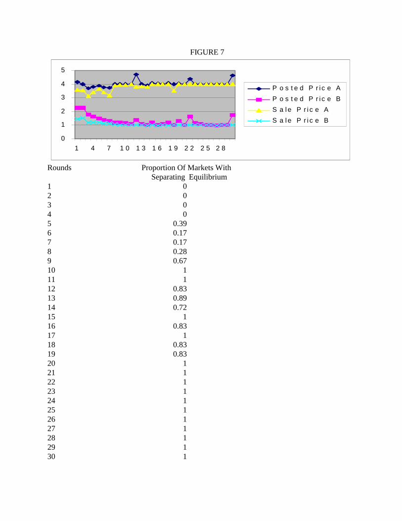
FIGURE 7

0

1

2

3

4

5

1 4 7 1 0 1 3 1 6 1 9 2 2 2 5 2 8



S a l e P r i c e A

S a l e P r i c e B


1 0 2 03 0 4 0 5 0.39 6 0.177 0.178 0.289 0.6710 1 11 1 12 0.8313 0.8914 0.7215 116 0.83 17 118 0.8319 0.83 20 1 21 1 22 1 23 1 24 1 25 1 26 1 27 1 28 1 29 1 30 1

FIGURE 8

0

1

2

3

4

5

1 4 7 1 0 1 3 1 6 1 9 2 2 2 5 2 8



S a l e P r i c e A

S a l e P r i c e B


1 0.33 2 03 0.174 0.175 0.336 0.177 0.398 0.789 0.510 0.511 0.6712 0.8313 0.8314 115 116 117 118 119 0.8320 121 122 123 124 125 126 0.8327 0.8328 129 130 1

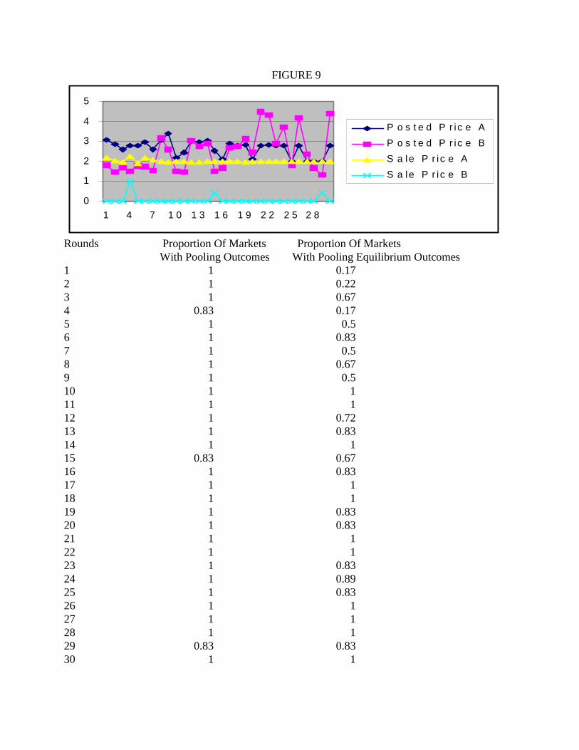
FIGURE 9

0

1

2

3

4

5

1 4 7 1 0 1 3 1 6 1 9 2 2 2 5 2 8



S a le P r i c e A

S a le P r i c e B

Rounds Proportion Of Markets Proportion Of Markets With Pooling Outcomes With Pooling Equilibrium Outcomes

1 1 0.172 1 0.223 1 0.674 0.83 0.175 1 0.56 1 0.837 1 0.58 1 0.679 1 0.510 1 111 1 112 1 0.7213 1 0.8314 1 115 0.83 0.6716 1 0.8317 1 118 1 119 1 0.8320 1 0.8321 1 122 1 123 1 0.8324 1 0.8925 1 0.8326 1 127 1 128 1 129 0.83 0.8330 1 1

FIGURE 10

0

1

2

3

4

5

6

1 4 7 1 0 1 3 1 6 1 9 2 2 2 5 2 8



S a le P r i c e A

S a le P r i c e B


1 0 02 0.33 0.173 0.33 04 0.5 05 0.33 06 0.5 0.177 0.67 0.178 0.17 09 0.17 010 0.33 0.1711 0.33 0.1712 0.67 013 0.33 0.1714 0.67 015 0.83 015 1 017 0.83 0.1718 0.83 0.2219 1 0.3320 1 0.3321 1 0.522 1 0.3923 1 0.6724 1 0.8325 1 126 1 127 1 0.6728 1 0.6729 1 130 1 0.72

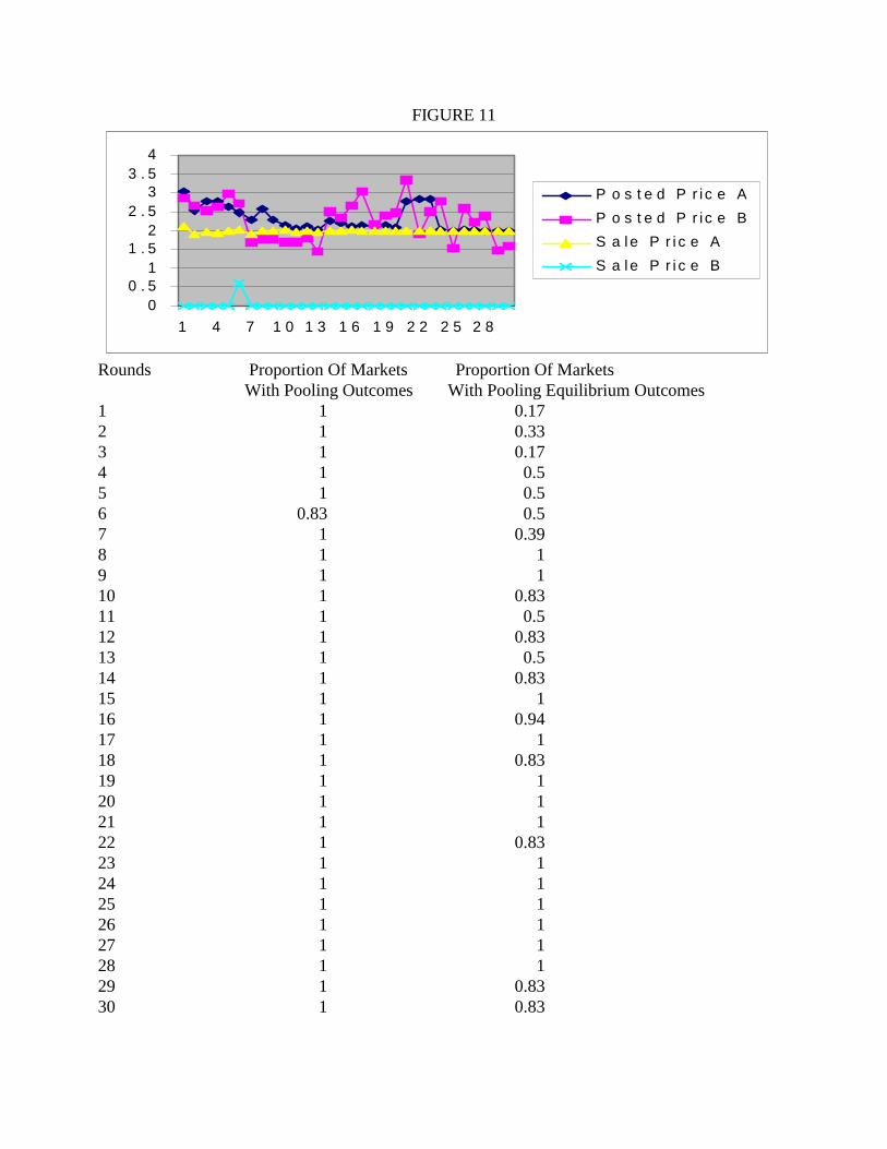
FIGURE 11

00 . 5

11 . 5

22 . 5

33 . 5

4

1 4 7 1 0 1 3 1 6 1 9 2 2 2 5 2 8



S a l e P r i c e A

S a l e P r i c e B


1 1 0.172 1 0.333 1 0.174 1 0.55 1 0.56 0.83 0.57 1 0.398 1 19 1 110 1 0.8311 1 0.512 1 0.8313 1 0.514 1 0.8315 1 116 1 0.94 17 1 118 1 0.8319 1 120 1 121 1 122 1 0.83 23 1 124 1 1 25 1 126 1 127 1 128 1 129 1 0.8330 1 0.83

Table 1. Statistical Tests For Session Effects for the Separating Treatment1

Using Data From Final RoundUsing Data From the last 15RoundsUsing Data From the All Rounds

Dependent Variable Observations Proportion ofequilibriumoutcomes

p-value2

Proportion of markets withSeparating Equilibrium in Session S1

18270540

1.956.763


18270540

1.967.720


18270540

1.967.734

Difference in Proportions(Session S1 - Session S2)

1.504.109


1.504.36


11

.493

1 The null hypothesis is that the Proportion of equilibrium prices is the same in both sessions.2 The reported p-value is the probability under the null hypothesis of getting a statistic as large

as the one observed.

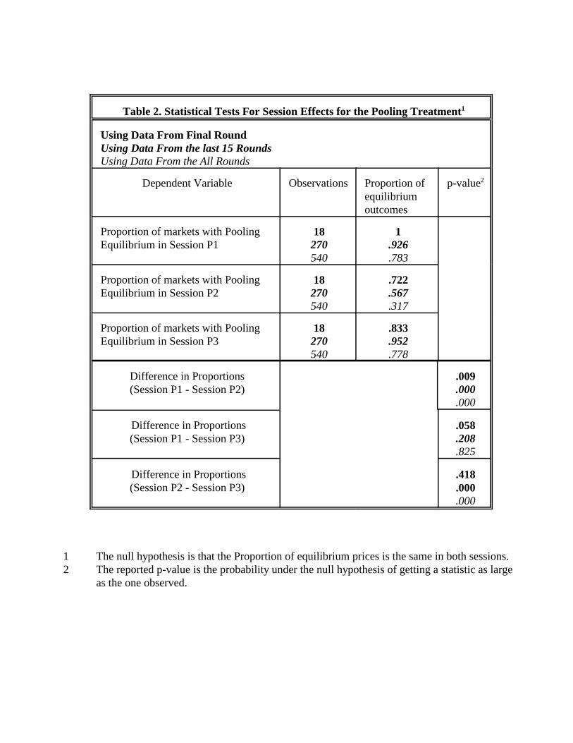
Table 2. Statistical Tests For Session Effects for the Pooling Treatment1

Using Data From Final RoundUsing Data From the last 15 RoundsUsing Data From the All Rounds

Dependent Variable Observations Proportion ofequilibriumoutcomes

p-value2

Proportion of markets with PoolingEquilibrium in Session P1

18270540

1.926.783

Proportion of markets with Pooling Equilibrium in Session P2

18270540

.722

.567

.317

Proportion of markets with Pooling Equilibrium in Session P3

18270540

.833

.952

.778

Difference in Proportions(Session P1 - Session P2)

.009

.000

.000


.058

.208

.825


.418

.000

.000

1 The null hypothesis is that the Proportion of equilibrium prices is the same in both sessions.2 The reported p-value is the probability under the null hypothesis of getting a statistic as large

as the one observed.

Table 3. A Comparison of the Separating and Pooling Sessions1

Round(s) Observations Number(proportion) of

SeparatingEquilibriumOutcomes inP1+P2+P3

Number(proportion) of

SeparatingEquilibriumOutcomesS1+S2+S3

p-value2

1-5 270 3 (.01) 38 (.14) 0

6-10 270 18 (.07) 152 (.56) 0

11-15 270 24 (.09) 230 (.85) 0

16-20 270 0 (0.0) 249 (.92) 0

21-25 270 0 (0.0) 270 (1.0)) 0

26-30 270 0 (0.0) 261 (.97) 0

16-30 810 0 (0.0) 780 (.96) 0

1-30 1610 45 (.03) 1200 (.74) 0

30 54 0 (0.0) 54 (1.0) 0

1 The null hypothesis is that the Proportion of separating equilibrium prices is the same insessions S1+S2+S3 and P1+P2+P3.

2 The reported p-value is the probability under the null hypothesis of getting a statistic as largeas the one observed.

FIGURE 1pL

p*

pH

CHL

CLE

Wealth inLoss State

Wealth in NoLoss State

45% Line

FIGURE 2pL

p*

pH

CHL

CLE

Wealth inLoss State


FIGURE 3pL

p*

pH

CHL

C’L

E

Wealth inLoss State


CH

FIGURE 4

p*

pH

CH

L

CLE

Wealth inLoss State


45% Line = IH

IL

pL

FIGURE 5pL

p*

pHCH

C’L

E

Wealth inLoss State


45% Line = IH

IL

H

FCL

CH

Screening Equilibria In Experimental Markets Lisa L. …aria.org/rts/proceedings/1999/posey_99.pdf2...

Documents

Transcript of Screening Equilibria In Experimental Markets Lisa L. …aria.org/rts/proceedings/1999/posey_99.pdf2...