Heriot-Watt University Research Gateway

Heriot-Watt University

Scoping prediction of re-radiated ground-borne noise and vibration near high speed rail lineswith variable soilsConnolly, David; Kouroussis, Georges; Woodward, Peter Keith; Giannopoulos, A; Verlinden,Olivier; Forde, Mike CPublished in:Soil Dynamics and Earthquake Engineering

DOI:10.1016/j.soildyn.2014.06.021

Publication date:2014

Document VersionEarly version, also known as pre-print

Link to publication in Heriot-Watt University Research Portal

Citation for published version (APA):Connolly, D., Kouroussis, G., Woodward, P. K., Giannopoulos, A., Verlinden, O., & Forde, M. C. (2014). Scopingprediction of re-radiated ground-borne noise and vibration near high speed rail lines with variable soils. DOI:10.1016/j.soildyn.2014.06.021

General rightsCopyright and moral rights for the publications made accessible in the public portal are retained by the authors and/or other copyright ownersand it is a condition of accessing publications that users recognise and abide by the legal requirements associated with these rights.

If you believe that this document breaches copyright please contact us providing details, and we will remove access to the work immediatelyand investigate your claim.

Download date: 23. Aug. 2018

1

1

Scoping prediction of re-radiated ground-borne noise and

vibration near high speed rail lines with variable soils

D.P. Connolly (corresponding author)1, G. Kouroussis2, P.K. Woodward1, A.

Giannopoulos1, O. Verlinden2 , M.C. Forde3

Abstract

This paper outlines a vibration prediction tool, ScopeRail, capable of predicting

in-door noise and vibration, within structures in close proximity to high speed railway

lines. The tool is designed to rapidly predict vibration levels over large track distances,

while using historical soil information to increase accuracy. Model results are

compared to an alternative, commonly used, scoping model and it is found that

ScopeRail offers higher accuracy predictions. This increased accuracy can potentially

reduce the cost of vibration environmental impact assessments for new high speed rail

lines.

To develop the tool, a three-dimensional finite element model is first outlined

capable of simulating vibration generation and propagation from high speed rail lines.

A vast array of model permutations are computed to assess the effect of each input

parameter on absolute ground vibration levels. These relations are analysed using a

machine learning approach, resulting in a model that can instantly predict ground

vibration levels in the presence of different train speeds and soil profiles. Then a

collection of empirical factors are coupled with the model to allow for the prediction of

structural vibration and in-door noise in buildings located near high speed lines.

Additional factors are also used to enable the prediction of vibrations in the presence of

abatement measures (e.g. ballast mats and floating slab tracks) and additional excitation

mechanisms (e.g. wheelflats and switches/crossings).

1. D.P. Connolly and P.K. Woodward, Heriot-Watt University, Edinburgh, UK

2. G. Kouroussis and O. Verlinden. Department of Theoretical Mechanics, Dynamics and Vibrations, University of Mons,Belgium

3. M.C. Forde and A. Giannopoulos, University of Edinburgh, Edinburgh, UK

2

2

KEYWORDS:

ScopeRail, High speed rail vibration, Environmental Impact Assessment (EIA), initial

vibration assessment, structural vibration, in-door noise, scoping assessment, high

speed train, urban railway

Highlights

Railway vibration scoping model developed to predict velocity decibel (VdB) levels

Model predicts ground/structural vibration and indoor noise for different soil types

Sub-model developed to utilize historical soil data for scoping vibration assessment

Model coupled to empirical factors to assess mitigation - ballast mats and floating slab

Model validated using 3 test sites and shown to outperform an alternative approach

3

3

1. Introduction

The rapid deployment of high speed rail (HSR) infrastructure has led to an increased

number of properties and structures being located in close proximity to high speed rail

lines (Carels, Ophalffens, & Vogiatzis, 2012), (D. P Connolly, Kouroussis, Laghrouche, Ho,

& Forde, 2014). In comparison to traditional inter-city rail, HSR speeds can potentially

generate elevated levels of vibration both within the track structure and in the free field.

In the free field these vibrations can impact negatively on the local environment,

causing properties to shake and walls/floors to generate indoor noise. This can result

in personal distress to those inhabiting such properties, and in the loss of building

functionality (e.g. for buildings sensitive to vibration such as hospitals, manufacturing

industries and places of worship (K Vogiatzis, 2010)).

Therefore in many countries, before a new line is constructed, it is compulsory to

undertake a vibration assessment exercise to identify the stakeholders that may

experience negative side-effects. To determine these stakeholders as early as possible,

the vibration levels from a new line must be calculated at the design stage. With the aim

of predicting vibration levels, much research has been undertaken into the analysis of

moving loads on a half-space (Fryba, 1972), (Kenney, 1954), (Andersen, Nielsen, &

Krenk, 2007). Alternatively, (Krylov, 1995) proposed a frequency domain model that

accounted for the contribution of each sleeper on the vibration field, and used Greens

functions to model ground wave propagation effects.

Alternative frequency domain approaches have since been proposed by (Sheng,

Jones, & Petyt, 1999), (Sheng, Jones, & Thompson, 2004) and (Konstantinos Vogiatzis,

2012) which used a combination of transfer functions for the train, track and soil to

calculate vibration levels, and at large distances from the track. (Auersch, 2012) also

used transfer functions to model the effect of moving loads and vibration through a

layered soil.

Other frequency domain approaches were presented by (M. F. M. Hussein & Hunt,

2009) and (M. F. M. Hussein & Hunt, 2007) who used the pipe-in-pipe (PiP) method to

predict vibration levels for underground railway lines. (Chebli, Othman, Clouteau,

Arnst, & Degrande, 2008), (Sheng, Jones, & Thompson, 2006) and (Galvin, Romero, &

Domínguez, 2010) also presented a three dimensional (3D) approach to modelling train

passage using a combination of the finite element (FE) and boundary element (BE)

method. The suitability of both the 3D FE-BE formulations and PiP approaches were

compared and found to perform well (Gupta, Hussein, Degrande, Hunt, & Clouteau,

2007).

Several time domain formulations have also been proposed for simulating railway

vibration. Although work has been undertaken to adapt the finite difference time

domain (FDTD) method for moving load problems (Thornely-Taylor, 2004), (Katou,

4

4

Matsuoka, Yoshioka, Sanada, & Miyoshi, 2008), the majority of research has been

performed using the FE method (and the coupled FE-BE method (Mulliken & Rizos,

2012)). Recently (Yang, Powrie, & Priest, 2009) presented a 2D FE analysis to

determine the effect of train speed on track characteristics. An alternative, advanced 3D

model was presented by (Kouroussis, Verlinden, & Conti, 2011) who used a sub-

structuring approach to model the propagation of vibration through the track, track and

soil. Similarly, (El Kacimi, Woodward, Laghrouche, & Medero, 2013) used a fully 3D FE

model to model vibrations from moving trains and analysed the effect of critical

velocities. Lastly,(D. Connolly, Giannopoulos, & Forde, 2013) used a fully 3D FE

approach to facilitate the modelling of the complex track geometry and its contribution

to railway vibration levels.

A challenge with both numerical frequency domain and numerical time domain

models is that their computational run times are prohibitive for initial scoping

assessment. If large sections of railway track require analysis then it is vital that

predictions can be made with low computational effort.

In an attempt to achieve this, (Rossi & Nicolini, 2003) proposed a straightforward

mathematical tool to rapidly predict soil absolute vibration velocity levels in decibels

and root mean squared values. The model only considered the contribution of Rayleigh

waves in its solution and the track was considered as a continuous structure. Results

were compared to field results obtained in (Harris, Miller, & Hanson, 1996) and it was

found that the modelling accuracy was comparable to more computationally demanding

numerical approaches.

An alternative model also based on the data collected in (Harris et al., 1996) was

developed by (Federal Railroad Administration, 2012) to predict absolute vibrations

from high speed rail lines. This empirical approach used curve fitting techniques to

develop relationships between train speed and distance from the track, with geological

conditions largely ignored. This curve was then adjusted based on empirically derived

factors to account for changes in soil-building coupling and track configuration.

This paper presents an empirically based model (ScopeRail) that builds upon (D. P

Connolly, Kouroussis, Giannopoulos, et al., 2014) to facilitate the prediction of vibration

decibels, in the presence of variable track-forms and in multiple building types.

Furthermore, new SPT relationships are defined to convert historical soil data into

model input data. The model uses a machine learning approach to approximate

relationships for the effect of soil layering on vibration transmission. These

relationships are then combined with empirical factors to facilitate rapid vibration

prediction for a wide array of track and building characteristics. ScopeRail is then

compared to the performance of the original (Federal Railroad Administration, 2012)

approach and it is found to offer enhanced performance.

5

5

2. MODELLING PHILOSOPHY Railway vibration scoping models are used to assess vibration levels quickly and

efficiently during the planning stage of a new line. Their goal is to predict vibration

levels across large sections of track (in a conservative manner) to identify key areas that

are likely to be effected by elevated vibration levels. Then these areas can then be

investigated further using more in-depth analysis. To predict vibration levels over wide

areas it is vital that scoping models can be deployed with minimal computational

requirements. With this in mind, accuracy is sometimes sacrificed in preference for

reduced computational requirements. This means that vibration levels can be often

overestimated and that detailed analysis is performed in areas where it was not

required. Detailed railway vibration analyses are cost intensive and therefore this

results in unnecessary additional project costs.

In addition to computational requirements and prediction accuracy, both parameter

availability and usability are important considerations when deploying a scoping

vibration prediction model. Usability is important from a practical point of view

because a model that has a long learning curve or requires extensive prior engineering

knowledge. Similarly, the model output must be compatible with the existing vibration

standards governing the project. Similarly, parameter availability is important because

if highly detailed soil information is needed for large areas then field experiments may

be required which is undesirable. Instead, for scoping assessment, it is more

advantageous to utilise rudimentary soil information in the form of historical records,

where possible, to quickly determine a simplified soil profile. For high speed lines, the

process of gathering historical soil data is performed at an early stage (for track

dynamics purposes) and therefore can also be utilised within a ground vibration

prediction model. These four equally desirable scoping model characteristics are

outlined in Figure 1.

Accuracy Execution time

UsabilityParameter

availability

6

6

Figure 1 – Vibration prediction models - development considerations

3. MODELLING APPROACH

The modelling approach used to develop ScopeRail was composed of two distinct

parts. Firstly a FE model was developed that was capable of predicting high speed

railway ground-borne vibration time histories. This model was then computed many

times to build up a database of velocity time histories for different soil conditions, train

speeds and distances from the track. The second step involved a statistical analysis of

results using a machine learning approach to achieve a model that could quickly and

accurately predict vibration levels in the presence of varying soil conditions.

3.1 FE model development The finite element model consisted of three distinct, fully coupled components to

describe the train, track and soil respectively. All components had one axis of symmetry

and therefore only half of each required modelling. The soil was modelled using linear

elastic, eight noded, three dimensional brick elements with dimensions 0.3m in each

direction. Four of the six soil boundaries were truncated using infinite elements,

described using an exponential decay function to simulate an infinitely long domain.

The top boundary was the location of the free surface and the horizontal displacement

was constrained in the direction perpendicular to the track thus accounting for the soil

symmetry. Rather than utilise a spherical geometry ((D. Connolly, Giannopoulos, &

Forde, 2013), (Kouroussis et al., 2011)) to improve infinite element performance, a

uniformly meshed rectangular model was preferred.

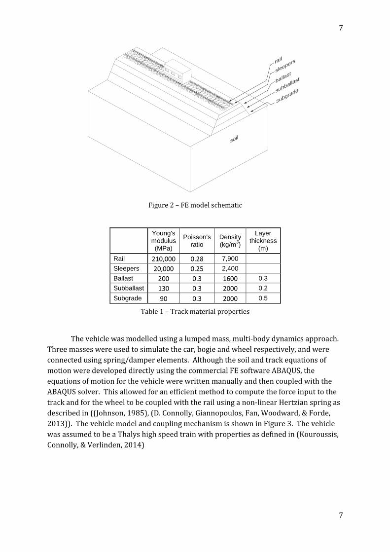
The track model was fully three dimensional (Figure 2) thus allowing for the

simulation of the complex geometries associated with its structure. This overcame

some of the assumptions associated with the simplified track modelling approaches as

presented by (Kouroussis et al., 2011), (El Kacimi et al., 2013). Therefore the

transmission of forces between each track component was simulated in a realistic

manner. The track conformed to the layout commonly found on high speed rail lines in

mainland Europe and was constructed from subgrade, subballast and ballast layers,

supporting evenly spaced sleepers at 0.6m spacings. The rail was connected to the

sleepers and modelled using 0.1m long beam elements. The track material properties

are show in Table 1.

7

7

Figure 2 – FE model schematic

Young's modulus (MPa)

Poisson's ratio

Density (kg/m3)

Layer thickness

(m)

Rail 210,000 0.28 7,900

Sleepers 20,000 0.25 2,400

Ballast 200 0.3 1600 0.3

Subballast 130 0.3 2000 0.2

Subgrade 90 0.3 2000 0.5

Table 1 – Track material properties

The vehicle was modelled using a lumped mass, multi-body dynamics approach.

Three masses were used to simulate the car, bogie and wheel respectively, and were

connected using spring/damper elements. Although the soil and track equations of

motion were developed directly using the commercial FE software ABAQUS, the

equations of motion for the vehicle were written manually and then coupled with the

ABAQUS solver. This allowed for an efficient method to compute the force input to the

track and for the wheel to be coupled with the rail using a non-linear Hertzian spring as

described in ((Johnson, 1985), (D. Connolly, Giannopoulos, Fan, Woodward, & Forde,

2013)). The vehicle model and coupling mechanism is shown in Figure 3. The vehicle

was assumed to be a Thalys high speed train with properties as defined in (Kouroussis,

Connolly, & Verlinden, 2014)

soil

subballastballast

subgrade

sleepersrail

8

8

Figure 3 – Vehicle model and coupling mechanism

3.2 ScopeRail model development Although the FE model could model railway tracks in detail and was able to

predict vibration time histories, its run times were too long for it to be used for railway

vibration scoping assessments. Therefore it was used as the basis to develop another

model, with much lower computational demands, known as ScopeRail. To do so, a

machine learning approach was used in an attempt to map train, track and soil

characteristics to resultant absolute ground vibration levels.

Firstly, a sensitivity analysis was undertaken to determine the most influential

parameters that contributed to the generation of ground borne vibration from rail lines.

The least influential parameters and those with large standard deviations (e.g.

wheel/rail defects) were excluded from model development. A more detailed

explanation of these tests can be found in (D. P Connolly, Kouroussis, Giannopoulos, et

al., 2014), (D. P Connolly, Peters, Sim, et al., 2014).

One of the most important parameters affecting ground vibration propagation is

soil characteristics (Auersch, 2012). To include soil properties within the scoping

model, two alternative approaches were undertaken. The first approach was to

consider the soil as a homogenous half space (i.e. a single layer) and the second was to

consider the soil as a two layer medium. It should be noted that although an infinite

number of soil configurations exist in practice, for the purpose of a scoping model, a

limited number of input parameters was desirable. This was because it is difficult to

obtain detailed soil information for large geographical areas. Therefore, extending the

model to three or more layers was considered undesirable. The key input/output

model parameters for the one layer and two layer cases are shown in Figure 4 and

Figure 5 respectively.

Additional

FORTRAN

solver

Default

ABAQUS

solver

Car

Bogie

Wheel

Sleeper

Rail

9

9

Figure 4 – One layer neural network schematic

Train

speed

Rayleigh

damping (B)

Young’s

modulus

Distance

VdB

Hidden

Layer

Input

Output

VdB

Young’s

modulus

(layer 1)

Rayleigh

damping (B)

Train

speed

Distance

Young’s

modulus

(layer 2)

Depth

(layer 1)

Hidden

Layer

Input

Output

10

10

Figure 5 – Two layer neural network schematic

3.3 Vibration metrics The complexity of seismic wave propagation prohibited the prediction of raw time

history signals using machine learning. Instead, key vibration indicators were

calculated using raw ABAQUS model vibration time histories and then used as the

outputs/targets for neural network construction.

Many national and international metrics have been proposed for railway

vibration assessment (Table 2). A challenge with their use is that each standard uses

different criteria to assess vibration levels making it difficult to compare standards and

to classify vibration levels universally. For example, the UK and Spain use acceleration

to quantify vibration whereas Germany and America use velocity criteria. Similar

differences exist between frequency weighting curves, time averaging procedures, units

of measurement and metrics. Comprehensive reviews of existing standards can be

found in (Griffin, 1998) and (Elias & Villot, 2011).

Although the scoping model outlined in (D. P Connolly, Kouroussis,

Giannopoulos, et al., 2014) was capable of predicting KBfmax (Deutsches Institut fur

Normung, 1999) and PPV values, these were less compatible with empirical vibration

relationships used to convert ground vibration into indoor noise. Therefore, with the

ultimate aim of maximising compatibility and usability, ScopeRail was redeveloped to

predict vibration decibels (VdBmax - hereafter denoted simply VdB) as outlined in

(Federal Railroad Administration, 2012). VdB was a logarithmic based vibration scale,

with the maximum value offering a useful individual absolute measurement of

vibration. It was calculated using Equation 1, where Vrms was the moving average of the

raw velocity time history, calculated over a one second time period (‘slow’ setting). V0

was the reference level of background vibration, for which a constant value of 2.54x10-6

m/s was chosen.

��� = 20 log�� ��

�� Equation 1

Country Relevant

standard(s) Country Relevant standard(s)

Austria ONORM 9012:2010 Spain Real Decreto

1307/2007

Germany DIN 4150-2:1999 Sweden SS 460 48 61:1992

Italy UNI 9614:1990 UK BS 6472-1:2008, BS

7385-2:1993

11

11

Netherlands SBR Richtlijn - Deel B

(2002) USA FRA (2012), FTA (2006)

Norway NS 8176:2005 International ISO 2631-1:1997, ISO

2631-2:2003

Table 2 - National and international vibration standards. (Recreated from (Elias & Villot, 2011)).

4. Using historical soil data within a scoping model

The advantage of ScopeRail over some alternative vibration scoping models was that

it was capable of accounting for soil conditions within its prediction. At the vibration

scoping stage of a high speed rail project rudimentary soil data is often available as a by-

product from track design/selection process. Therefore this information can be reused

within a scoping model. Despite this, if a comprehensive record of soil data is not

available then it may be necessary to construct soil profiles manually from historical

information. These historical records usually relate to tests such as borehole logs and

SPT, which are not directly compatible with the properties required to model wave

propagation. Therefore, it is difficult to utilise historical data within previously

developed models such as (D. P Connolly, Kouroussis, Giannopoulos, et al., 2014).

To overcome this, a variety of previously proposed empirical relationships were

investigated for the purpose of mapping the most common types of exiting historical

test records to wave propagation parameters. These relationships were used to

develop a range of new equations, which were then incorporated within ScopeRail.

4.1 Utilising historical SPT data An advantage of using Standard Penetration Test (SPT) N-values to determine FE

modelling properties is that historically the SPT test has been the most widely

performed test and national resources such as (“British Geological Association,” 2013)

provide an extensive database of borehole logs. Therefore it is often possible to obtain

SPT data without the financial outlay required to perform physical tests.

Additionally, a wide body of research exists for correlating SPT N-values with

physical soil properties. Therefore it is possible to use SPT data to obtain soil

properties that are more reliable than using soil only description data. Despite this, a

challenge with the SPT test is that the methodology is not performed consistently and

parameters such as the drop height can vary between countries. (Robertson,

Campanella, & Wightman, 1983) presented correction factors to account for these

inconsistencies although some authors have questioned whether these factors lead to

more reliable results. Additionally, it should be noted that all SPT N-value correlations

12

12

are based on soils experiencing low strain levels (i.e. the assumption of small strain

theory).

Figure 6 presents correlations between SPT N-values and shear wave speeds for

general soils. The overall deviation between correlations is low, apart from (Seed,

Idriss, & Arango, 1983) and (Iyisan, 1996), which both seem to overestimate shear wave

velocity.

Figure 6 - SPT shear wave velocity correlations – all soils. (Seed et al., 1983), (Imai & Tonouchi,

1982), (Sisman, 1995), (Ohta & Goto, 1978), (Hasancebi & Ulusay, 2006), (Iyisan, 1996)

Rather than use SPT correlations to classify all generic soil types, empirical

relationships have also been presented for individual soil types. Each of these is based

upon whether the soil is a sand, clay or silt; information which is typically recorded

when performing SPT testing.

Figure 7, Figure 8 and Figure 9 show relationships for sand, silt and clay

respectively. For each soil type, relationships are relatively well correlated with each

alternative relationship. Exceptions are the relationships proposed by (Jafari, Shafiee, &

Razmkhah, 2002), which for each soil, overestimates the shear wave velocity.

In addition to the relationships shown in Figure 6 - Figure 9, authors such as

(Seed, Wong, Idriss, & Tokimatsu, 1987) have proposed correlations based on a greater

number of variables (e.g. soil depth) in attempt to improve accuracy.

0 50 100 150 200 250 3000

100

200

300

400

500

600

700

800

900

1000

SPT blows

She

ar w

ave

velo

city

(m

/s)

Seed et al., 1983Imai and Tonouchi, 1982Sisman, 1995Ohta and Goto, 1987Hasancebi and Ulusay, 2007Iyisan, 1996Best fit

13

13

Figure 7 - SPT correlations – Sand. (Hasancebi & Ulusay, 2006), (Imai, 1977), (S. Lee, 1990), (S.

Lee, 1990), (Pitilakis, Raptakis, Lontzetidis, & T, 1999), (Tsiambaos & Sabatakakis, 2010)

Figure 8 - SPT correlations – Silt. (Jafari et al., 2002), (C. Lee & Tsai, 2008), (Pitilakis et al., 1999),

(Tsiambaos & Sabatakakis, 2010)

0 50 100 150 200 250 3000

100

200

300

400

500

600

700

800

900

1000

SPT blows

She

ar w

ave

velo

city

(m

/s)

Hasancebi and Ulusay, 2007Sykora and Stokoe, 1982Imai, 1977Lee, 1990Pitilakis, 1999Tsiambaos et al. 2011Best fit

0 50 100 150 200 250 3000

200

400

600

800

1000

1200

1400

1600

1800

SPT blows

She

ar w

ave

velo

city

(m

/s)

Jafari et al., 2002Lee, 2008Pitilakis, 1999Tsiambaos et al., 2011Best fit

14

14

Figure 9 - SPT correlations – Clay. (Hasancebi & Ulusay, 2006), (S. Lee, 1990), (Jafari et al.,

2002), (Pitilakis et al., 1999), (Tsiambaos & Sabatakakis, 2010)

Rather than attempt to utilise a variety of SPT relationships, one new relationship for

each soil type was developed. These new relationships were best fit correlations

between all other relationships and are shown using a black line in Figure 6 - Figure 9.

For both the silt and clay relationships, the equations presented by (Jafari et al., 2002)

were ignored because they exhibited a poor correlation with all other proposed

relationships. The new relationships are described numerically in Table 3 and plotted

in Figure 10. As expected, the SPT relationships proposed for generic soil shear wave

speeds had the largest standard deviation. Silts had a relatively large standard

deviation and clays had the lowest at 64.5m/s.

Soil type SPT relationship Standard deviation

(m/s)

General soils Vs = 62.9 ∙ N 0.425 111.7

Sands Vs = 86.71 ∙ N 0.3386 81.6

Clays Vs = 120.8 ∙ N 0.2865 64.5

Silts Vs = 127.1 ∙ N 0.2595 102.9

Table 3 - Best fit SPT ‘N-value’ correlations

0 50 100 150 200 250 3000

200

400

600

800

1000

1200

1400

1600

1800

SPT blows

She

ar w

ave

velo

city

(m

/s)

Hasancebi and Ulusay, 2007Lee, 1990Jafari et al., 2002Pitilakis, 1999Tsiambaos et al., 2011Best fit

15

15

Figure 10 - Best fit SPT ‘N-value’ correlations

4.2 Utilising historical CPT data The Cone Penetration Test (CPT) test is an alternative and more sophisticated

penetration experiment in which a metal cone is pushed into soil and the penetrative

resistance (qc) is measured. The cone typically has a diameter of 35.7mm2, cast at a 600

angle and is pushed, with the aid of a land vehicle, into the soil at a constant rate.

It addition to cone tip resistance, sleeve friction (fs) is commonly measured. Less

commonly, piezocone penetration tests are used to measure pore water pressure and

sometimes seismic cone penetration tests are used to measure shear wave velocity.

Although CPT testing is becoming more widespread, SPT testing remains more

common place and historical data relating to SPT N-values is more freely available. One

explanation for this is that due to the force required to push the cone into soils, the CPT

method can only be used for relatively soft soils. Therefore researchers such as (Chin,

Duann, & Kao, 1988) have attempted to correlate CPT results with SPT N-values. This

approach is not recommended for the purpose of using empirical correlations to

estimate FE parameters because it creates an additional layer of uncertainty. Instead,

several authors have presented formulations based directly on CPT results, a variety of

which are shown in Table 4.

For these relationships, σ is effective stress, ‘k2’ is a coefficient function of

relative density, ‘qt’ is the corrected cone tip resistance (Dejong, 2007) and ‘e0’ is void

ratio. The relationships have not been plotted graphically because of their dependence

on a variety of soil parameters. This makes it challenging to make direct comparisons.

0 50 100 150 200 250 3000

100

200

300

400

500

600

700

800

SPT blows

She

ar w

ave

velo

city

(m

/s)

General soilsSandsClaysSilts

16

16

Soil property Equation Soil type Reference

Shear

modulus 1000 ∙ k2 ∙ σ 0.5 Sand

(Paoletti, Hegazy,

Monaco, & Piva,

2010)

Shear wave

velocity 50 ∙ ((qc/pa)0.43 - 3) Sand

(Paoletti et al.,

2010)

Shear wave

velocity 277 ∙ qt

0.13 ∙ σ 0.27 Sand

(Baldi, Bellotti,

Ghionna,

Jamiolkowski, &

Presti, 1989)

Shear wave

velocity

(10.1 ∙ log(qt) - 11.4)1.67 ∙

(fs/qt ∙ 100)0.3

General soils (Hegazy & Mayne,

1995)

Shear wave

velocity 118.8 ∙ log(fs) + 18.5 General soils (Mayne, 2006)

Shear wave

velocity 1.75 ∙ qt

0.627 Clay (Mayne & Rix,

1995)

Shear wave

velocity 9.44 ∙ qt 0.435 ∙ e0

-0.532 Clay (Mayne & Rix,

1993)

Shear wave

velocity 1.75 ∙ qt 0.627 Clay

(Mayne & Rix,

1993)

Table 4 - CPT empirical relationships

4.3 Utilising historical laboratory data Lab testing involves extracting soil samples from the test site, transporting them to the

lab and performing controlled experiments to determine characteristics that are

difficult to obtain using in-situ tests.

A variety of lab testing methodologies are available including bender element

testing, resonant column testing, ultrasonic pulse testing and more traditionally, tri-

axial testing.

17

17

A major advantage of lab testing is that the samples are tested under controlled

conditions and therefore allow for a more accurate determination of soil properties.

Despite this, due to inevitable sample disturbances caused during soil sample extraction

and transportation, the properties of a soil at the time of lab testing are not always

similar to the properties of the soil in-situ.

Classical lab testing refers to tests such as the quick undrained triaxial test to

determine undrained shear strength (Dickensen, 1994). They also include other tests to

determine properties such as bulk density, moisture content, liquid limit and plastic

limit. Although these soil properties (except density) are not required for FE

simulation, correlations have been proposed to map them more closely to parameters

such as Young’s modulus (Houbrechts et al., 2011).

For vibration prediction purposes, it is sometimes the case that classical lab

testing data is available in addition to existing borehole data. Therefore empirical

correlations between lab data and FE parameters may be useful for validating SPT

correlations. Despite this, if a new soil lab investigation is being performed then bender

element and resonant column testing techniques are preferable to classical lab testing.

This is because the aforementioned tests can determine FE parameters directly, rather

than approximating them using empirical relationships.

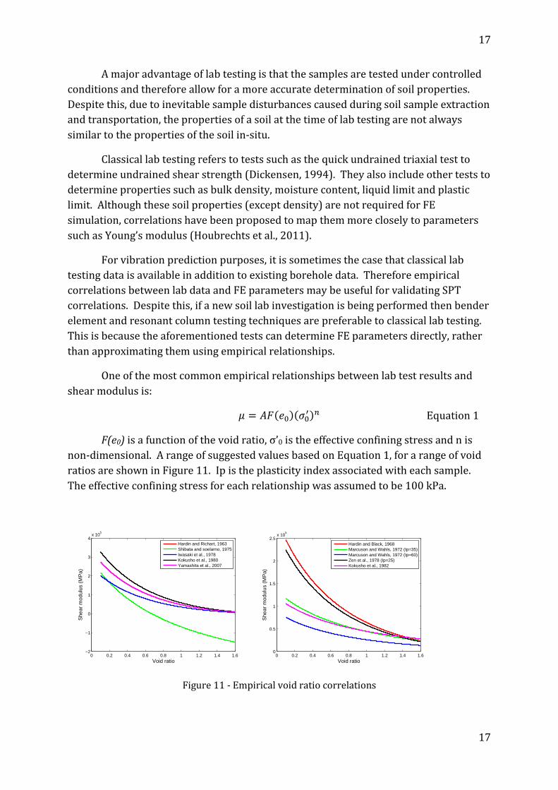
One of the most common empirical relationships between lab test results and

shear modulus is:

� = ������������ Equation 1

F(e0) is a function of the void ratio, σ’0 is the effective confining stress and n is

non-dimensional. A range of suggested values based on Equation 1, for a range of void

ratios are shown in Figure 11. Ip is the plasticity index associated with each sample.

The effective confining stress for each relationship was assumed to be 100 kPa.

Figure 11 - Empirical void ratio correlations

0 0.2 0.4 0.6 0.8 1 1.2 1.4 1.6−2

−1

0

1

2

3

4x 10

5

Void ratio

She

ar m

odul

us (

MP

a)

Hardin and Richart, 1963Shibata and soelarno, 1975Iwasaki et al., 1978Kokusho et al., 1980Yamashita et al., 2007

0 0.2 0.4 0.6 0.8 1 1.2 1.4 1.60

0.5

1

1.5

2

2.5x 10

5

Void ratio

She

ar m

odul

us (

MP

a)

Hardin and Black, 1968Marcuson and Wahls, 1972 (Ip=35)Marcuson and Wahls, 1972 (Ip=60)Zen et al., 1978 (Ip=25)Kokusho et al., 1982

18

18

Equation 1 depends solely on the prior calculation of void ratio and therefore is

often used due to its ease of application. Alternatively, researchers have presented

formulations which depend on additional experimentally calculated variables. For

example, (Larsson & Mulabdic, 1991) outlined a correlation based upon liquid limit and

undrained shear strength. Also, (Hardin & Black, 1963) presented a correlation based

upon both void ratio and over-consolidation ratio (OCR). Despite this OCR is difficult to

accurately determine even through lab testing thus making it difficult for practical use.

Some empirical relationships for calculating OCR from CPT results are provided by

(Lunne, Robertson, & Powell, 1997).

Damping can also be calculated from classical lab test results with (Kramer,

1996) suggesting it can be calculated using the hystersis loop for a soil. Alternatively,

several authors propose that damping is highly correlated with normalised shear

modulus. As discussed previously, vibrations generated due to train passage are in the

small strain zone thus allowing (Ishibashi & Zhang, 1993) to propose the relationship:

� = 0.0065�1 + ���.� !"#$.%� Equation 4.2

This equation is based on solely the plastic modulus (Ip) and has been shown by

(Biglari & Ashayeri, 2011) to provide an accurate approximation for a range of soils.

Alternative formulations have also been presented by (Rollins, Evans, Diehl, & Daily,

1998) and (Kagawa, 1993), both based on using cyclic shear strain values.

Furthermore, (Houbrechts et al., 2011) presented typical damping values for soil

(Figure 12).

0 1 2 3 4 5 6 7

Clay

Gravel

Sand

Material damping (%)

19

19

Figure 12 – Typical damping ratios (replicated from (Houbrechts et al., 2011))

4.4 Soil layer mapping

The scoping model was only capable computing a discrete number of input soil

layers (2 layers), however typical soil profiles consist of a greater number of layers.

Therefore, to enable the model to be used at any test site, the soil property input

information was converted into a 2 layer soil. This translation was performed using a

straightforward thickness weight average technique:

'() =∑+,',

∑+,

Equation 3

where Eeq = equivalent Young’s modulus, Hi = each layer thickness and Ei = Young’s

modulus of each layer.

5. Structural vibration, mitigation and excitation factors

The machine learning approach allowed for rapid prediction of ground vibrations in

two layered soils. Additionally, the empirical soil relationships allowed for historical

soil relationships to be included in the vibration propagation path. Despite this, the

upgraded machine learning approach was based upon results obtained from a generic

high speed train-track-soil model, and it could only predict absolute vibration levels on

a soil surface.

To upgrade ScopeRail versatility from the previously developed approach (D. P

Connolly, Kouroussis, Giannopoulos, et al., 2014), and make it applicable to a wider

range of track forms and excitation mechanisms, it was combined with empirical

modification factors (Federal Railroad Administration, 2012). These factors allowed for

the vibration level to be modified to account for elevated excitations generated due to

wheelflats, corrugated track and switches/crossings. Similarly, the factors allowed for

the vibration levels to be modified to account for ballast mats, floating slabs, resilient

fasteners/ties and earthworks profiles. Although more detailed structural factors have

been proposed (Auersch, 2010), the use of transfer functions within a scoping model

adds undesired complexity. Furthermore, because the (Federal Railroad

Administration, 2012) amplification factors were essentially uncoupled, and the

vibration metric (VdB) was the same as that used within ScopeRail, the compatibility

between methods was high. This facilitated a seemless coupling between the factors

and ScopeRail.

20

20

Furthermore, as the original FE model was only used to predict ground surface

vibration levels rather than building vibrations, the basic ScopeRail model could also

only predict ground vibration levels. This is a commonly used approach ((Lombaert &

Degrande, 2009), (Kouroussis et al., 2011), (Kattis, Polyzos, & Beskos, 1999), (Sheng et

al., 1999), (Galvin et al., 2010), (Auersch, 2012), (Costa, Calçada, & Cardoso, 2012),

(O’Brien & Rizos, 2005)) due to the difficulties in determining soil-building coupling

characteristics. Although several attempts have been made to include soil-structure

coupling within predictions ((Fiala, Degrande, & Augusztinovicz, 2007), (M. Hussein,

Hunt, Kuo, Costa, & Barbosa, 2013)), these methods are still experimental. To convert

the ScopeRail predicted ground vibration levels to structural vibration and in-door

noise, empirical modification factors were again used (Federal Railroad Administration,

2012).

It should be noted that the factors related to train speed, distance from the track and

geologicial conditions were not retained from the (Federal Railroad Administration,

2012) procedure. This is because these factors were inherently included within the

ScopeRail model. The final factors implemented with ScopeRail are shown in the

Appendix.

6. Model validation

6.1 Field work To ensure that the scoping model was capable of predicting vibration levels for a

variety of test sites and that it had not been over-fitted, it was validated using three sets

of experimental results. To provide a fair comparison, these field test results were

composed of data collected by the authors and also by independent researchers.

The first set of results were recorded in Belgium in 2001 (Degrande & Schillemans,

2001) and thus denoted ‘Degrande 2001’. During testing, vibration levels were sampled

using accelerometers and then converted to velocity time histories. A more detailed

experimental description is found in the original article.

An experimental campaign was also undertaken in 2012 to collect results for the

additional comparisons. Firstly, vibrations were recorded on the Paris to Brussels high

speed line (David P. Connolly, 2014), (Kouroussis, Connolly, Forde, & Verlinden, 2013),

(D. P Connolly, Kouroussis, Fan, et al., 2013) and were denoted ‘Mons 2012’. Secondly,

vibrations were recorded on the London-Paris high speed line (HS1) and were denoted

‘HS1 2012’. Identical equipment was used for both experimental tests, however for the

‘Mons 2012’ tests, vibrations were measured up to 100m from the track, while for the

‘HS1 2012’ tests, vibrations were measured up to 35m from the track. For both tests a

21

21

multi-channel analysis of surface waves procedure was used to determine the

underlying soil properties (Figure 14). For each train passage the train speed was

determined during post-processing using a combination of cepstral analysis, dominant

frequency analysis and a regression analysis to compare experimental and theoretical

frequency spectrum (Kouroussis, Connolly, Forde, & Verlinden, 2014).

Figure 13 – left: ‘Mons 2012’ test site, Right: ‘HS1 2012’ test site.

Figure 14 – Compressional and shear wave profiles at test sites, Left: Degrande 2001, Middle:

Mons 2012, Right: HS1 2012

6.2 One layer model validation First the model was tested using a homogenous soil to approximate the layered

profile at each test site. To benchmark the model performance against a scoping model

that did not include soil properties in its calculation, the results were compared to

predictions calculated using the (Federal Railroad Administration, 2012) approach.

Figure 15 shows that the homogenous model performed well and was able to

predict VdB values with strong accuracy for each test site. For the Mons 2012 test site

ScopeRail closely matched the experimental results. Similar results were found for

Degrande 2001 although there was an over prediction of vibration levels for the

receivers at distances greater than 10m. For the HS1 2012 results the new model was

found to slightly over predict vibration levels at distances less than 20-25m from the

track, and to over predict levels at further distances.

0 100 200 300 400 5000

5

10

15

Wave velocity (m/s)

Soi

l dep

th (

m)

P waveS wave

0 200 400 600 800 10000

5

10

15

Wave velocity (m/s)

Soi

l dep

th (

m)

P waveS wave

0 500 1000 1500 20000

5

10

15

Wave velocity (m/s)

Soi

l dep

th (

m)

P waveS wave

22

22

A comparison between models revealed that performance was relatively similar,

with both models overestimating vibration levels for the majority of receiver locations.

For the (Federal Railroad Administration, 2012) calculations, this reflects the

anticipated conservative nature of the model. For the Mons 2012 results, ScopeRail was

found to offer marginally enhanced performance at large offsets (2-3 dB), and

moderately better accuracy for HS1 2012.

Figure 15 - One layer model performance, Top left: Mons 2012 (291 km/h), Top right: Mons

2012 (294 km/h), Bottom left: Degrande 2001 (271 km/h), Bottom right: HS1 2012 (270km/h)

6.3 Two layer model validation The two layer ScopeRail model was also tested against the experimental data and

the (Federal Railroad Administration, 2012) approach. Figure 16 shows that again both

models over-predicted vibration levels. Despite this, ScopeRail performed with

increased accuracy in comparison to when the homogenous soil profile was used. This

is particularly clear for the Degrande 2001 results where a significant improvement is

obtained (up to 9-10dB). For the Mons 2012 results enhanced accuracy was also found.

0 20 40 60 80 10060

65

70

75

80

85

90

Mons 2012 (294km/h)

Distance from track (m)

Ve

loci

ty (

Vd

B)

Field experiment

ScopeRail

FRA 2012

0 20 40 60 80 10060

65

70

75

80

85

90

95

100

Degrande 2001 (271km/h)

Distance from track (m)

Ve

loci

ty (

Vd

B)

Field experiment

ScopeRail

FRA 2012

0 20 40 60 80 10075

80

85

90

95

HS1 2012 (270km/h)

Distance from track (m)

Ve

loci

ty (

Vd

B)

Field experiment

ScopeRail

FRA 2012

0 20 40 60 80 10060

65

70

75

80

85

90

Mons 2012 (291km/h)

Distance from track (m)

Ve

loci

ty (

Vd

B)

Field experiment

ScopeRail

FRA 2012

23

23

In comparison to the (Federal Railroad Administration, 2012) approach,

ScopeRail was found to outperform it for the Mons 2012 and Degrande 2001 test sites,

however performance was still low for both models at the HS1 2012 site. This increase

in accuracy was attributed to the additional degrees of freedom available within the 2

layer ScopeRail model.

Figure 16 – Two layer model performance, Top left: Mons 2012 (291 km/h), Top right: Mons

2012 (294 km/h), Bottom left: Degrande 2001 (271 km/h), Bottom right: HS1 2012 (270km/h)

6.4 DISCUSSION ScopeRail was found to offer strong vibration prediction performance, particularly

when the 2 layer soil model was used. Prediction accuracy was highest for the Mons

2012 and Degrande 2001 test sites because the change in vibration levels with distance

was relatively uniform, thus making these sites more straightforward to predict. In

comparison, the HS1 2012 data set contained vibration levels with large amplitude

unexpected local increases. It was challenging for the numerical model to predict these

anomalies, however the scoping model was able to generate results that corresponded

well to a best-fit line through the results. Therefore it was concluded that the new

model offered improved performance in comparison to (Federal Railroad

Administration, 2012).

0 20 40 60 80 10060

65

70

75

80

85

90

Mons 2012 (291km/h)

Distance from track (m)

Ve

loci

ty (

Vd

B)

Field experiment

ScopeRail

FRA 2012

0 20 40 60 80 10060

65

70

75

80

85

90

95

100

Degrande 2001 (271km/h)

Distance from track (m)

Ve

loci

ty (

Vd

B)

Field experiment

ScopeRail

FRA 2012

0 20 40 60 80 10060

65

70

75

80

85

90

Mons 2012 (294km/h)

Distance from track (m)

Ve

loci

ty (

Vd

B)

Field experiment

ScopeRail

FRA 2012

0 20 40 60 80 10075

80

85

90

95

HS1 2012 (270km/h)

Distance from track (m)

Ve

loci

ty (

Vd

B)

Field experiment

ScopeRail

FRA 2012

24

24

7. CONCLUSIONS

A tool designed for the scoping assessment of in-door noise caused by high speed

train passage was developed. Firstly, a three-dimensional numerical model capable of

simulating vibration generation and propagation from high speed rail lines was

outlined. This model was executed many times, each time using a different combination

of input parameters, to create a database of results. These results were then analysed

using a neural network approach to determine the effect of parameter changes on

vibration levels. This resulted in a model that could instantly predict ground vibration

levels in the presence of different train speeds and soil profiles. Finally, a collection of

empirical factors were added to the model to facilitate the prediction of structural

vibration and in-door noise in buildings located near high speed lines. The final model

is called ScopeRail and was shown to offer increased accuracy over an alternative

scoping model.

The advantage of this increased accuracy is that it reduces the probability of

under and over prediction of vibration levels. If levels are over predicted then

unnecessary detailed vibration assessments will be needed for further analysis. If levels

are under predicted then abatement measures may be required post line construction.

Therefore higher accuracy predictions can result in substantial cost savings.

8. ACKNOWLEDGEMENTS

The authors wish to thank the University of Edinburgh, the University of Mons and

Heriot Watt University for the support and resources provided for the undertaking of

this research. Additionally, the funding provided by Engineering and Physical Sciences

Research Council (EP/H029397/1) and the Natural Environment Research Council is

also greatly appreciated, without which, this research could not have been undertaken.

It should also be noted that a selection of the experimental field results mentioned in

this work can be found at www.davidpconnolly.com.

9. References

Andersen, L., Nielsen, S. R. K., & Krenk, S. (2007). Numerical methods for analysis of

structure and ground vibration from moving loads. Computers & Structures, 85(1-

2), 43–58. doi:10.1016/j.compstruc.2006.08.061

25

25

Auersch, L. (2010). Building Response due to Ground Vibration — Simple Prediction

Model Based on Experience with Detailed Models and Measurements. International

Journal of Acoustics and Vibration, 15(3), 101–112.

Auersch, L. (2012). Train induced ground vibrations: different amplitude-speed

relations for two layered soils. Proceedings of the Institution of Mechanical

Engineers, Part F: Journal of Rail and Rapid Transit, 226(5), 469–488.

doi:10.1177/0954409712437305

Baldi, G., Bellotti, R., Ghionna, V., Jamiolkowski, M., & Presti, D. (1989). Modulus of sands

from CPT’s and DMT's. In 12th International conference on Soil Mechanics and

Foundation Engineering (pp. 165–170).

Biglari, M., & Ashayeri, I. (2011). An empirical model for shear modulus and damping

ratio of unsaturated soils. Unsaturated Soils: Theory and Practice, 1, 591–595.

British Geological Association. (2013). Retrieved from http://www.bgs.ac.uk/

Carels, P., Ophalffens, K., & Vogiatzis, K. (2012). Noise and Vibration evaluation of a

floating slab in direct fixation turnouts in Haidari & Anthoupoli extensions of

Athens metro lines 2 and 3. INGEGNERIA FERROVIARIA, 533–552.

Chebli, H., Othman, R., Clouteau, D., Arnst, M., & Degrande, G. (2008). 3D periodic BE–FE

model for various transportation structures interacting with soil. Computers and

Geotechnics, 35(1), 22–32. doi:10.1016/j.compgeo.2007.03.008

Chin, C., Duann, S., & Kao, T. (1988). SPT-CPT correlations for granular soils. In 1st

International symposium on Penetration Testing (pp. 295–339).

Connolly, D., Giannopoulos, A., Fan, W., Woodward, P. K., & Forde, M. C. (2013).

Optimising low acoustic impedance back-fill material wave barrier dimensions to

shield structures from ground borne high speed rail vibrations. Construction and

Building Materials, 44, 557–564. doi:10.1016/j.conbuildmat.2013.03.034

Connolly, D., Giannopoulos, A., & Forde, M. C. (2013). Numerical modelling of ground

borne vibrations from high speed rail lines on embankments. Soil Dynamics and

Earthquake Engineering, 46, 13–19. doi:10.1016/j.soildyn.2012.12.003

Connolly, D. P. (2014). High Speed Rail Dataset. Retrieved from

http://www.davidpconnolly.com/

Connolly, D. P., Kouroussis, G., Fan, W., Percival, M., Giannopoulos, A., Woodward, P. K., …

Forde, M. C. (2013). An experimental analysis of embankment vibrations due to

high speed rail. In Proceedings of the 12th International Railway Engineering

Conference.

Connolly, D. P., Kouroussis, G., Giannopoulos, A., Verlinden, O., Woodward, P. K., & Forde,

M. C. (2014). Assessment of railway vibrations using an efficient scoping model. Soil

26

26

Dynamics and Earthquake Engineering, 58, 37–47.

doi:10.1016/j.soildyn.2013.12.003

Connolly, D. P., Kouroussis, G., Laghrouche, O., Ho, C., & Forde, M. C. (2014).

Benchmarking Railway Vibrations - Track, Vehicle, Ground and Building Effects

(accepted paper). Construction and Building Materials - Special Issue: Railway

Engineering.

Connolly, D. P., Peters, J., Sim, A., Giannopoulos, A., Forde, M. C., Kouroussis, G., &

Verlinden, O. (2014). Railway vibration impact assessment-High accuracy and

internationally compatible tool. In Proceedings of the Transportation Research

Board 93rd Annual meeting, Washington (USA).

Costa, P. A., Calçada, R., & Cardoso, A. S. (2012). Ballast mats for the reduction of railway

traffic vibrations. Numerical study. Soil Dynamics and Earthquake Engineering, 42,

137–150. doi:10.1016/j.soildyn.2012.06.014

Degrande, G., & Schillemans, L. (2001). Free Field Vibrations During the Passage of a

Thalys High-Speed Train At Variable Speed. Journal of Sound and Vibration, 247(1),

131–144. doi:10.1006/jsvi.2001.3718

Dejong, J. (2007). Site characterization - Guidelines for estimating Vs based on In-situ

tests. Soil interaction laboratory, UCDavis (pp. 1–22).

Deutsches Institut fur Normung. (1999). DIN 4150-2 - Human exposure to vibration in

buildings. International Standards Organisation (pp. 1–63).

Dickensen, S. (1994). Dynamic response of soft and deep cohesive soils during the Loma

Prieta earthquake of October 17, 1989. PhD thesis. University of California.

El Kacimi, A., Woodward, P. K., Laghrouche, O., & Medero, G. (2013). Time domain 3D

finite element modelling of train-induced vibration at high speed. Computers &

Structures, 118, 66–73. doi:10.1016/j.compstruc.2012.07.011

Elias, P., & Villot, M. (2011). Review of existing standards, regulations and guidelines , as

well as laboratory and field studies concerning human exposure to vibration.

Deliverable D1.4. (RIVAS) (pp. 1–72).

Federal Railroad Administration. (2012). High-Speed Ground Transportation Noise and

Vibration Impact Assessment. U.S. Department of Transportation (pp. 1–248).

Fiala, P., Degrande, G., & Augusztinovicz, F. (2007). Numerical modelling of ground-

borne noise and vibration in buildings due to surface rail traffic. Journal of Sound

and Vibration, 301(3-5), 718–738. doi:10.1016/j.jsv.2006.10.019

Fryba, L. (1972). Vibration of Solids and Structures Under Moving Loads (pp. 1–524).

Groningen, The Netherlands: Noordhoff International Publishing.

27

27

Galvin, P., Romero, A., & Domínguez, J. (2010). Fully three-dimensional analysis of high-

speed train–track–soil-structure dynamic interaction. Journal of Sound and

Vibration, 329(24), 5147–5163. doi:10.1016/j.jsv.2010.06.016

Griffin, M. (1998). A Comparison of Standardized Methods for Predicting the Hazards of

Whole-Body Vibration and Repeated Shocks. Journal of Sound and Vibration,

215(4), 883–914. doi:10.1006/jsvi.1998.1600

Gupta, S., Hussein, M., Degrande, G., Hunt, H. E. M., & Clouteau, D. (2007). A comparison

of two numerical models for the prediction of vibrations from underground railway

traffic. Soil Dynamics and Earthquake Engineering, 27(7), 608–624.

doi:10.1016/j.soildyn.2006.12.007

Hardin, B., & Black, W. (1963). Vibration modulus of normally consolidated clay. Journal

of the Soil Mechanics and Foundation Division, 89, 33–65.

Harris, Miller, & Hanson. (1996). Summary of European high speed rail noise and

vibration measurements (HMMH Report No. 293630-2) (pp. 1–158).

Hasancebi, N., & Ulusay, R. (2006). Empirical correlations between shear wave velocity

and penetration resistance for ground shaking assessments. Bulletin of Engineering

Geology and the Environment, 66(2), 203–213. doi:10.1007/s10064-006-0063-0

Hegazy, Y., & Mayne, P. (1995). Statistical correlations between Vs and CPT data for

different soil types. In (CPT’95), Symposium on Cone Penetration Testing (pp. 173–

178).

Houbrechts, J., Schevenels, M., Lombaert, G., Degrande, G., Rucker, W., Cuellar, V., &

Smekal, A. (2011). Test procedures for the determination of the dynamic soil

characteristics. (RIVAS - Deliverable D1.1) (pp. 1–107).

Hussein, M. F. M., & Hunt, H. E. M. (2007). A numerical model for calculating vibration

from a railway tunnel embedded in a full-space. Journal of Sound and Vibration,

305(3), 401–431. doi:10.1016/j.jsv.2007.03.068

Hussein, M. F. M., & Hunt, H. E. M. (2009). A numerical model for calculating vibration

due to a harmonic moving load on a floating-slab track with discontinuous slabs in

an underground railway tunnel. Journal of Sound and Vibration, 321(1-2), 363–374.

doi:10.1016/j.jsv.2008.09.023

Hussein, M., Hunt, H. E. M., Kuo, K., Costa, P. A., & Barbosa, J. (2013). The use of sub-

modelling technique to calculate vibration in buildings from underground railways.

Proceedings of the Institution of Mechanical Engineers, Part F: Journal of Rail and

Rapid Transit. doi:10.1177/0954409713511449

Imai, T. (1977). P and S-wave velocities of the ground in Japan. In Ninth International

conference of Soil Mechanics and Foundation Engineering (pp. 257–260).

28

28

Imai, T., & Tonouchi, K. (1982). Correlation of N-value with S-wave velocity and shear

modulus. In Proceedings of the 2nd European symposium of penetration testing (pp.

57–72).

Ishibashi, I., & Zhang, X. (1993). Unified dynamic shear moduli and damping ratios of

sand and clay. Soils and Foundations, 33(1), 182–191.

Iyisan, R. (1996). Correlations between shear wave velocity and in-situ penetration test

results. Teknik Dergi, 7(2), 1187–1199.

Jafari, M., Shafiee, A., & Razmkhah, A. (2002). Dynamic properties of fine grained soils in

south of Tehran. Journal of Seismology and Earthquake Engineering, 4(1), 25–35.

Johnson, K. (1985). Contact mechanics (pp. 1–468). Cambridge, UK: Cambridge

University Press.

Kagawa, T. (1993). Moduli and damping factors of soft marine clays. Journal of

Geotechnical Engineering, 118(9), 1360–1375.

Katou, M., Matsuoka, T., Yoshioka, O., Sanada, Y., & Miyoshi, T. (2008). Numerical

simulation study of ground vibrations using forces from wheels of a running high-

speed train. Journal of Sound and Vibration, 318, 830–849.

doi:10.1016/j.jsv.2008.04.053

Kattis, S., Polyzos, D., & Beskos, D. (1999). Vibration isolation by a row of piles using a 3-

D frequency domain BEM. International Journal for Numerical Methods in

Engineering, 728(February), 713–728.

Kenney, J. (1954). Steady-state vibrations of beam on elastic foundation for moving

load. Journal of Applied Mechanics, 76, 359–364.

Kouroussis, G., Connolly, D. P., Forde, M. C., & Verlinden, O. (2013). An experimental

study of embankment conditions on high-speed railway ground vibrations. In

International congress on Sound and Vibration (pp. 1–8). Bangkok, Thailand.

Kouroussis, G., Connolly, D. P., Forde, M. C., & Verlinden, O. (2014). Train speed

calculation using ground vibrations. Proceedings of the Institution of Mechanical

Engineers, Part F: Journal of Rail and Rapid Transit, 0(0), 1–18.

doi:10.1177/0954409713515649

Kouroussis, G., Connolly, D. P., & Verlinden, O. (2014). Railway induced ground

vibrations - a review of vehicle effects. International Journal of Rail Transportation,

2(2), 69–110. doi:10.1080/23248378.2014.897791

Kouroussis, G., Verlinden, O., & Conti, C. (2011). Free field vibrations caused by high-

speed lines: Measurement and time domain simulation. Soil Dynamics and

Earthquake Engineering, 31(4), 692–707. doi:10.1016/j.soildyn.2010.11.012

Kramer, S. (1996). Geotechnical earthquake engineering (pp. 1–653). Prentice Hall.

29

29

Krylov, V. (1995). Generation of ground vibrations by superfast trains. Applied Acoustics,

44(2), 149–164. doi:10.1016/0003-682X(95)91370-I

Larsson, R., & Mulabdic, M. (1991). Shear moduli in Scandinavian clays; measurements

of initial shear modulus with seismic cones - empirical correlations for the initial

shear modulus in clay. In Transport Reasearch Board (pp. 1–127).

Lee, C., & Tsai, B. (2008). Mapping Vs30 in Taiwan. Terrestrial Atmospheric and Oceanic

Sciences, 19(6), 671–682. doi:10.3319/TAO.2008.19.6.671(PT)1.

Lee, S. (1990). Regression models of shear wave velocities in Taipei basin. Journal of the

Chinese Institution of Engineers, 13(5), 519–1990.

Lombaert, G., & Degrande, G. (2009). Ground-borne vibration due to static and dynamic

axle loads of InterCity and high-speed trains. Journal of Sound and Vibration, 319,

1036–1066. doi:10.1016/j.jsv.2008.07.003

Lunne, T., Robertson, P., & Powell, J. (1997). Cone penetrating testing (pp. 1–312). Spons

Press.

Mayne, P. (2006). Undisturbed sand strength from seismic cone tests. Geomechanics &

Geoengineering, 1(4), 239–257.

Mayne, P., & Rix, G. (1993). Gmax-qc Relationships for Clays. ASTM Geotechnical Testing

Journal, 16(1), 54–60.

Mayne, P., & Rix, G. (1995). Correlations Between Shear Wave Velocity and Cone Tip

Resistance in Clays. Soils and Foundations, 35(2), 107–110.

Mulliken, J., & Rizos, D. C. (2012). A coupled computational method for multi-solver,

multi-domain transient problems in elastodynamics. Soil Dynamics and Earthquake

Engineering, 34(1), 78–88. doi:10.1016/j.soildyn.2011.10.004

O’Brien, J., & Rizos, D. (2005). A 3D BEM-FEM methodology for simulation of high speed

train induced vibrations. Soil Dynamics and Earthquake Engineering, 25, 289–301.

doi:10.1016/j.soildyn.2005.02.005

Ohta, Y., & Goto, N. (1978). Empirical shear wave velocity equations in terms of

characteristic soil indexes. Earthquake Engineering & Structural Dynamics, 6(2),

167–187.

Paoletti, L., Hegazy, Y., Monaco, S., & Piva, R. (2010). Prediction of shear wave velocity

for offshore sands using CPT data – Adriatic sea. In 2nd International Symposium on

Cone Penetration Testing (pp. 1–8). Huntington Beach, California.

Pitilakis, K., Raptakis, D., Lontzetidis, K., & T, T.-V. (1999). Geotechnical and geophysical

description of EURO-SEISTEST, using field, laboratory tests and moderate strong

motion recordings. Journal of Earthquake Engineering, 3(3), 381–409.

30

30

Robertson, P., Campanella, G., & Wightman, A. (1983). SPT-CPT correlations. Journal of

Geotechnical Engineering, 109(11), 1449–1459.

Rollins, K., Evans, M., Diehl, N., & Daily, W. (1998). Shear Modulus And Damping

Relationships For Gravels. Journal of Geotechnical and Geoenvironmental

Engineering, 124(5), 396–405.

Rossi, F., & Nicolini, A. (2003). A simple model to predict train-induced vibration:

theoretical formulation and experimental validation. Environmental Impact

Assessment Review, 23(3), 305–322. doi:10.1016/S0195-9255(03)00005-2

Seed, H., Idriss, I., & Arango, I. (1983). Evaluation Of Liquefaction Potential Using Field

Performance Data. Journal of Geotechnical Engineering, 109, 458–482.

Seed, H., Wong, R., Idriss, I., & Tokimatsu, K. (1987). Moduli and Damping Factors for

Dynamic Analyses of Cohesionless Soils. Journal of Geotechnical Engineering,

112(11), 1016–1032.

Sheng, X., Jones, C. J. C., & Petyt, M. (1999). Ground Vibration Generated By a Harmonic

Load Acting on a Railway Track. Journal of Sound and Vibration, 225(1), 3–28.

doi:10.1006/jsvi.1999.2232

Sheng, X., Jones, C. J. C., & Thompson, D. J. (2004). A theoretical model for ground

vibration from trains generated by vertical track irregularities. Journal of Sound and

Vibration, 272(3-5), 937–965. doi:10.1016/S0022-460X(03)00782-X

Sheng, X., Jones, C., & Thompson, D. (2006). Prediction of ground vibration from trains

using the wavenumber finite and boundary element methods. Journal of Sound and

Vibration, 293(3-5), 575–586. doi:10.1016/j.jsv.2005.08.040

Sisman, H. (1995). An investigation on relationships between shear wave velocity and SPT

and pressuremeter test results (MSc thesis). Ankara University.

Thornely-Taylor, R. M. (2004). The Prediction Of Vibration , Groundborne And

Structure-Radiated Noise From Railways Using Finite Difference Methods – Part I -

Theory. In Proceedings of the Institute of Acoustics (Vol. 26, pp. 1–11).

Tsiambaos, G., & Sabatakakis, N. (2010). Empirical estimation of shear wave velocity

from in situ tests on soil formations in Greece. Bulletin of Engineering Geology and

the Environment, 70(2), 291–297. doi:10.1007/s10064-010-0324-9

Vogiatzis, K. (2010). Noise & Vibration theoretical evaluation & monitoring program for

the protection of the ancient “Kapnikarea Church” from Athens Metro Operation.

International Review of Civil Engineering (I.RE.C.E.), 1(5), 328–333.

Vogiatzis, K. (2012). Environmental ground borne noise and vibration protection of

sensitive cultural receptors along the Athens Metro Extension to Piraeus. Science of

the Total Environment, 439, 230–7. doi:10.1016/j.scitotenv.2012.08.097

31

31

Yang, L. A., Powrie, W., & Priest, J. A. (2009). Dynamic Stress Analysis of a Ballasted

Railway Track Bed during Train Passage. Journal of Geotechnical and

Geoenvironmental Engineering, 135(5), 680. doi:10.1061/(ASCE)GT.1943-

5606.0000032

Appendix Source factor Adjustment to ScopeRail results

Worn wheels of wheel flats + 10 dB

Worn or corrugated track + 10 dB

Crossovers or other special track work + 10 dB

Table A. 1 – ScopeRail source factors (replicated from (Federal Railroad Administration,

2012))

Track factor Adjustment to ScopeRail results

Floating slab track bed - 15 dB

Ballast Mats - 10 dB

High resilience fasteners - 5 dB

Resiliently supported sleepers - 10 dB

Type of track structure (relative to at-grade

tie and ballast) Ariel/Viaduct structure - 10 dB

Embankment 0 dB

Open cutting 0 dB

Type of track structure (relative to bored

tunnel in soil) Station - 5 dB

Cut and cover - 3 dB

Rock-based - 15 dB

Table A. 2 – ScopeRail track factors (replicated from (Federal Railroad Administration, 2012))

Receiver factor Adjustment to ScopeRail results

Coupling to building foundation Wood frame - 5 dB

1-2 Story masonry - 7 dB

2-4 Story masonry - 10 dB

Large masonry (piled) - 10 dB

Large masonry (spread) - 13 dB

Foundation in rock 0 dB

Floor-to-floor attenuation Storeys 1-5 above grade - 2 dB per floor

Storeys 5-10 above grade - 1 dB per floor

Amplification due to resonances of floors,

walls and ceilings + 6 dB

32

32

Radiated sound Typical at-grade track - 50 dB

Typical tunnelled track - 35 dB

Tunnel in rock - 20 dB

Table A. 3 – ScopeRail receiver factors (replicated from (Federal Railroad Administration,

2012))