
SCHOOL OF ENGINEERING DEPARTMENT OF MECHANICAL...
80
UNIVERSITY OF NAIROBI SCHOOL OF ENGINEERING DEPARTMENT OF MECHANICAL AND MANUFACTURING ENGINEERING COMPUTER AIDED DESIGN OF V-BELT AND CHAIN DRIVES PROJECT INDEX: MFO 05/2011 PRESENTED BY CHRISTOPHER MUREMWA KIRONJI F18/1814/2006 THAIRU STANLEY NG’ANG’A F18/9249/2005 SUPERVISOR: PROF M.F. ODUORI PROJECT REPORT SUBMITTED IN PARTIAL FULFILMENT OF THE REQUIREMENT FOR THE AWARD OF THE DEGREE OF BACHELOR OF SCIENCE IN MECHANICAL ENGINEERING, THE UNIVERSITY OF NAIROBI SUBMITTED ON: 3 RD JUNE 2011
Transcript of SCHOOL OF ENGINEERING DEPARTMENT OF MECHANICAL...
UNIVERSITY OF NAIROBI
SCHOOL OF ENGINEERING
DEPARTMENT OF MECHANICAL AND MANUFACTURING ENGINEERING
COMPUTER AIDED DESIGN OF V-BELT AND CHAIN DRIVES
PROJECT INDEX: MFO 05/2011
PRESENTED BY
CHRISTOPHER MUREMWA KIRONJI F18/1814/2006
THAIRU STANLEY NG’ANG’A F18/9249/2005
SUPERVISOR: PROF M.F. ODUORI
PROJECT REPORT SUBMITTED IN PARTIAL FULFILMENT OF THE REQUIREMENT FOR THE
AWARD OF THE DEGREE
OF
BACHELOR OF SCIENCE IN MECHANICAL ENGINEERING,
THE UNIVERSITY OF NAIROBI
SUBMITTED ON: 3RD
JUNE 2011

i
DECLARATION
Students
This report is our original work and has not been published or presented for award of
degree in any university there before.
Signed………………………………………
Date…………………………………………
CHRISTOPHER MUREMWA KIRONJI
Signed...…………………………………
Date……………………………………..
THAIRU STANLEY NG’ANG’A
Supervisor
This report has been submitted by the above students for examination with my
approval as a university lecturer and supervisor of the project.
Signed…………………………………..
Date…………………………………….
PROF M.F. ODUORI

Page | ii
DEDICATION
We would like to dedicate this project to our dear parents, siblings and friends for the moral
and material support they have accorded to us through our academic life and their effort to
seeing us pursue our dreams towards attaining a higher education.

Page | iii
ACKNOWLEDGEMENTS
Would like to express our sincere and utmost gratitude to the following individuals, without
whose assistance and constant supervision, this project would never have been completed.
First and foremost, we express our heartfelt gratitude to our supervisor Dr. MF Oduori, for all
the guidance and time he had made available towards the completion of this project. Not to
forget also the materials assistance he had made available to us in terms of books and other
forms of information he afforded to us.
Last but not the least; we would like to thank the university fraternity, our friends and family
for their endless support during this time.
May God bless you all.
S.Thairu and C.Kironji
Page | iv
Table of Contents DECLARATION.......................................................................................................................................... i
DEDICATION............................................................................................................................................. ii
ACKNOWLEDGEMENTS ...................................................................................................................... iii
ABSTRACT ................................................................................................................................................. 1
PART 1: INTRODUCTION ...................................................................................................................... 2
CHAPTER ONE ......................................................................................................................................... 2
1. INTRODUCTION ...................................................................................................................... 2
1.1. DESIGN .................................................................................................................................. 2
1.2. COMPUTER-AIDED ENGINEERING & DESIGN (C.A.E & C.A.D) ................................ 3
PART 2: LITERATURE REVIEW .......................................................................................................... 5
CHAPTER TWO ........................................................................................................................................ 5
2. REVIEW OF LITERATURE ON V-BELTS AND V-BELTS DESIGN ................................... 5
2.1. HISTORY / ORIGIN AND DEVELOPMENTS OF V-BELTS ............................................ 5
2.2. STRUCTURE OF A V-BELT ................................................................................................ 7
2.3. PARTS OF A V-BELT ........................................................................................................... 8
2.4. V-BELT DRIVES ................................................................................................................... 8
2.4.1. STRUCTURE OF A V-BELT DRIVE ............................................................................... 9
2.4.2. TYPES OF BELT DRIVE SYSTEMS ............................................................................ 10
2.4.3. DEFINITION OF TERMS USED IN BELT DRIVES .................................................. 11
2.4.4 THEORY OF BELT DRIVES ......................................................................................... 12
CHAPTER THREE .......................................................................................................................... 14
3. REVIEW OF LITERATURE ON DEVELOPMENT OF A COMPUTER AIDED DESIGN
FOR V-BELTS / V-BELT DRIVES ................................................................................................. 14
3.1. INTRODUCTION ................................................................................................................ 14
3.2. DESIGN PROCESS .............................................................................................................. 14
3.3. COMPUTER AIDED DESIGN OF V-BELTS .................................................................... 20
3.3.1. How to create a C.A.D from Matlab program (method) ................................................... 21
3.3.1.1. Algorithms used in Matlab ............................................................................................ 23
3.3.2. Developing a GUI for v-belt design program ................................................................... 26
CHAPTER FOUR ............................................................................................................................. 30
4. REVIEW OF LITERATURE ON CHAINS, CHAIN DRIVES AND COMPUTER AIDED
DESIGN OF CHAIN DRIVES ......................................................................................................... 30
4.1. INTRODUCTION TO CHAINS .......................................................................................... 30
4.2. MECHANICS OF CHAIN DRIVES ................................................................................... 32

Page | v
4.3. DESIGN OF A ROLLER CHAIN DRIVE ........................................................................... 34
4.3.1. Number of teeth in sprockets ............................................................................................ 34
4.3.2. Drive Ratio ........................................................................................................................ 36
4.3.3. Drive Arrangements .......................................................................................................... 36
4.3.4 Shafts Centre Distance ............................................................................................................... 37
4.3.3.1. Centre Distance Adjustment ......................................................................................... 38
4.3.3.2. Chain lubrication ........................................................................................................... 39
4.4. SELECTION PROCEDURE FOR CHAIN DRIVES WITH TWO SPROCKETS ............. 41
4.5. COMPUTER AIDED DESIGN OF CHAIN DRIVES ......................................................... 45
4.5.1. Developing a graphical user interface (GUI) .................................................................... 46
PART THREE: CASE STUDY ............................................................................................................... 49
CHAPTER FIVE ...................................................................................................................................... 49
5. CASE STUDY ON THE APPLICATION OF THE V-BELT AND CHAIN DRIVE DESIGN
PROGRAM FOR A SISAL DECORTICATOR MACHINE ........................................................... 49
5.1. INTRODUCTION ................................................................................................................ 49
5.2. DESIGN DATA .................................................................................................................... 49
5.3. APPLICATION / USING THE PROGRAM ........................................................................ 52
CHAPTER SIX ......................................................................................................................................... 57
6. CLOSURE ................................................................................................................................ 57
6.1. DISCUSSION OF RESULTS ............................................................................................... 57
6.2. CONCLUSION ..................................................................................................................... 58
6.3. RECOMMENDATIONS ...................................................................................................... 58
1
ABSTRACT
The aim of this project is to develop a computer aided design program for the selection of v-
belt and chain drives. It encompasses simplifying the bulky and time consuming process of
using tables and charts into a simplified user friendly program.
Before the creation of this program, proper review of the selection procedure of v-belts and
chain drives was carried out in order to understand the most important aspects of design.
Once determined it was important to code them in a machine language that the computer can
interpret .This involved the generation of equations from design charts in order to fully
computerize the process. This was done in the case of determination of power rating for v-
belt drives where equations were generated for belt sections A to E conforming to ANSI
standard classifications. In cases where equations could not be developed, tables were
provided whereby specific values needed were to be input by the user in the final program.
These included service factors and correction factor.
Matlab programming language was used to develop the source code and an executable
program. This was chosen because it is a scripting programming language applicable in most
engineering applications and is easy to understand. The complete code used for the design
program is provided in the appendix.
To ascertain the accuracy of the program created, a case study was done to determine the
appropriate belt drive and also chain drive for use on a sisal decorticator machine and the
results obtained were compared with values obtained earlier using theoretical calculations,
charts and tables. The motor rating for the sisal decorticator studied was 1.5 kW, 600mm
center distance, service factor of 1.1. Using design charts the appropriate belt drive
determined was an ANSI standard B section, driven diameter of 183.6mm, driving diameter
of 135mm, belt length of 1703.7mm, and number of belt 1. For the chains, the driving
sprocket, 22 teeth, driven sprocket, 30 teeth, chain pitch length of 152.02~152 pitches. Using
the program an appropriate belt drive would be of ANSI standard B section, 183.5mm driven
diameter, 135mm driving diameter and belt length of 1703.1mm whereas for chain drives the
pitch length was found to be 152.2~152 pitches for using an ANSI standard chain of ⅜
inch(9.525mm) pitch.
Page | 2
PART 1: INTRODUCTION
CHAPTER ONE
1. INTRODUCTION
1.1. DESIGN
To design is either to formulate a plan for the satisfaction of a specified need or to solve a
problem. If the plan results in the creation of something having a physical reality, then the
product must be functional, safe, reliable, competitive, usable, manufactureable and
marketable.
Design is an innovative and highly iterative process. It is also a decision-making process.
Decisions sometimes have to be made with too little information, occasionally with just the
right amount of information, or with an excess of partially contradictory information.
Decisions are sometimes made tentatively, with the right reserved to adjust as more becomes
known. The point is that the engineering designer has to be personally comfortable with a
decision-making, problem-solving role.
Design is a communication-intensive activity in which both words and pictures are used, and
written and oral forms employed. Engineers have to communicate effectively and work with
people of many disciplines. These are important skills, and an engineer`s success depends on
them.
A designer`s personal resources of creativity, communicative ability, and problem solving
skill are intertwined with knowledge of technology and first principles. Engineering tools
(such as mathematics, statistics, computers, graphics, and languages) are combined to
produce a plan that ,when carried out, produces a product that is functional, safe, reliable,
competitive, useable, manufactureable, and marketable, regardless of who builds it or who
uses it .1
The design process includes these steps:
1. Recognition of need.
2. Formulation of specifications, that is, conformance of product to need of designer.
3. Creative synthesis (creativity, invention, imaginative combination of parts to form a
new design/product).
4. Drafting.
1 Refer; Shigley`s Mechanical Engineering Design 8
th edition Chapter 1 Design pg 4-5

Page | 3
5. Analyzing (determining stresses and deflections, and comparing them with strength
and acceptable deflection.)
6. Redesigning as required.
7. Manufacturing and testing.
1.2. COMPUTER-AIDED ENGINEERING & DESIGN (C.A.E & C.A.D)
Computer aided engineering is the practice of engineering with help of using computers.
Engineering is a wide discipline of science and involves various branches/fields of practices
such as nuclear, mechanical, civil & structural and many more.
Each field of practice in engineering involves various scientific theories, calculations,
formulas, equipments of use and other properties. Frequently engineering practice involves
problem solving and decision making to conform to certain desired outcomes/solutions to
problems. The use of computers in engineering design enables the pre-programming and
customization ability of engineering aspects into a program/database of various properties for
use.
Similar to computer aided engineering is computer-aided design or drafting (CAD).It is here
where software packages (such as; Matlab, Windows excel, Auto CAD…) take advantage of
the computer’s ability to store, process data and retrieve information.
A designer describes the proposed design and then displays it on the computer monitor as an
output image, user interface or even a plot. Design changes can be made quickly and
inexpensively at this point. Furthermore, CAD can be used to create an accurate three
dimensional (3-D) geometry /shape, database, produce a bill of materials, and to eliminate the
need for a prototype, or create a prototype via stereo-lithography2.Thus CAD can reduce
concept-to-production time, improving competitiveness3.
The importance of (CAE) is that it allows flexibility in decision making. During design, there
may be need to try altering the design to check outcomes limited by certain considerations.
For example, how to reduce costs incurred in designing? What can be adjusted to increase
efficiency? What is the end result if a given dimension is changed?
C.A.E may also involve various procedures of how to implement it in an engineering
firm/plant. For example;
Series approach; where C.A.E is practiced based on a sequence of steps following
each other.
However it is important to recognize the highly efficient method of concurrent engineering.
An Institute for Defense Analysis report (1986) defines concurrent engineering (CE) as “a
systematic approach to integrated, concurrent design of products and their related processes.
2 A rapid prototyping method particularly suited to parts with complex geometry.
3Refer; Computer Integrated Machine Design By Charles E .Wilson Creative design chapter 1 pg 2-3

Page | 4
CE requires teamwork and coordination involving research and development engineers,
designers, manufacturing engineers and technicians, and personnel from other functions.
The focus is on product-based teams rather than on departments. With CE aspects of product
design and development can be carried out simultaneously. Thus, CE is a parallel process,
while the traditional process is a series approach. Problems sometimes result from lack of co-
ordination in the traditional approach. CE attempts to eliminate such problems in the concept
and design phase.’’

Page | 5
PART 2: LITERATURE REVIEW
CHAPTER TWO
2. REVIEW OF LITERATURE ON V-BELTS AND V-BELTS DESIGN
2.1. HISTORY / ORIGIN AND DEVELOPMENTS OF V-BELTS
The V-belt was developed in 1917 by John Gates of the Gates rubber Company. They are
generally endless, and their general cross-section shape is trapezoidal. The V-shape of the
belt tracks in a mating groove in the pulley (sheave), with the result that the belt cannot slip
off. The belt tends to wedge into the groove as the load increases-the greater the load, the
greater the wedging action-improving torque transmission and making the v-belt an effective
solution, needing less width and tension than flat belts.4
Belt Definition; a flexible non-metallic member (Friction Belt drives by, Prof. M.F. Oduori)
A V-belt is a type of belt drive classification in which the belt drives cross sections are
trapezoidal.
Belt drives are a type of flexible machine element used in various industrial applications for
power transmission. The belt is looped over pulleys and is used to link motion between the
two pulleys from the driving pulley (motor shaft) to the driven pulley.
There are also various types of other belts, such as;
Cogged belts
Fig 2.1a
4 Courtesy of www.wikipedia.org-belt(mechanical)
Page | 6
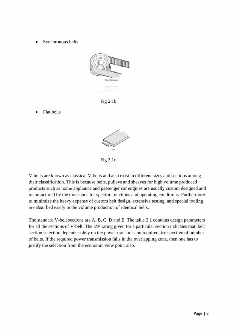
Synchronous belts
Fig 2.1b
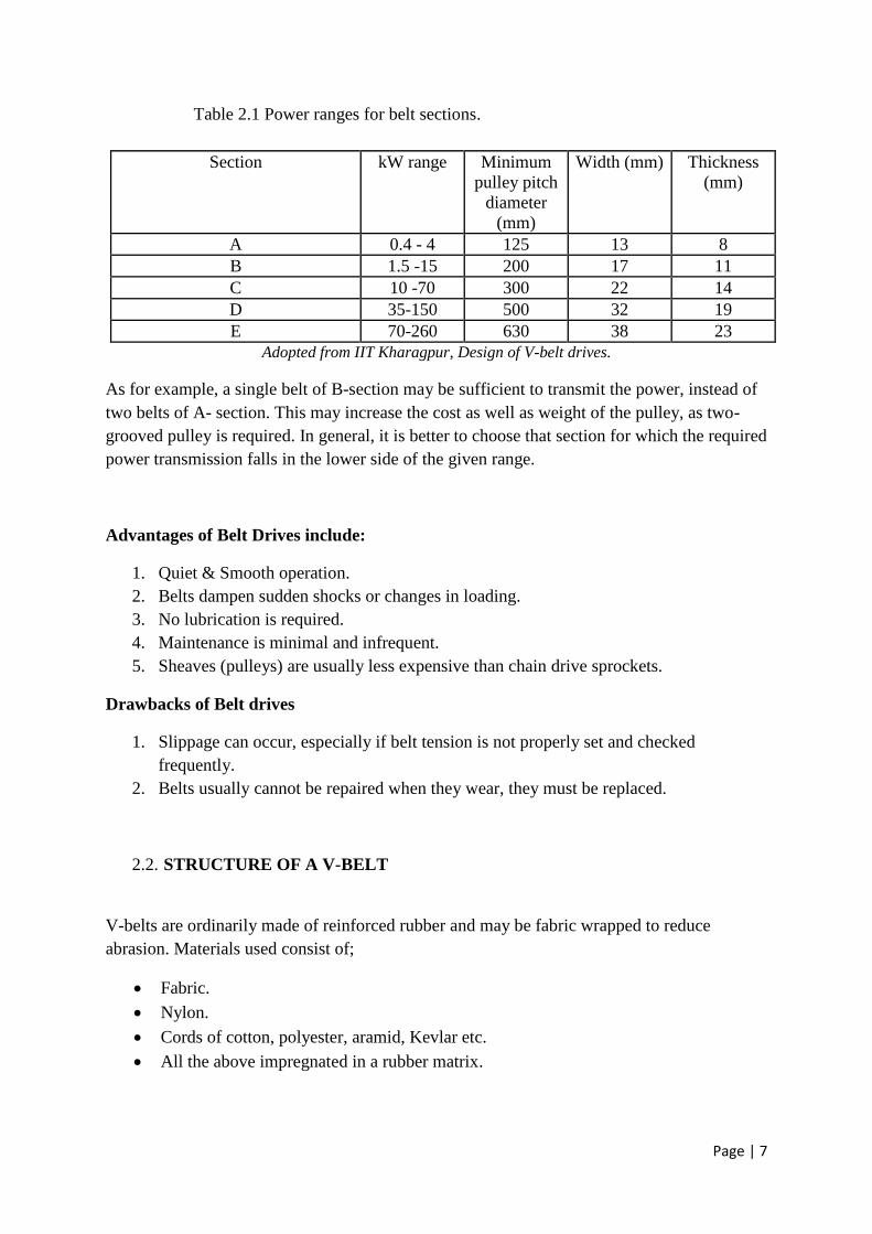
Flat belts
Fig 2.1c
V-belts are known as classical V-belts and also exist in different sizes and sections among
their classification. This is because belts, pulleys and sheaves for high volume produced
products such as home appliance and passenger car engines are usually custom designed and
manufactured by the thousands for specific functions and operating conditions. Furthermore
to minimize the heavy expense of custom belt design, extensive testing, and special tooling
are absorbed easily in the volume production of identical belts.
The standard V-belt sections are A, B, C, D and E. The table 2.1 contains design parameters
for all the sections of V-belt. The kW rating given for a particular section indicates that, belt
section selection depends solely on the power transmission required, irrespective of number
of belts. If the required power transmission falls in the overlapping zone, then one has to
justify the selection from the economic view point also.
Page | 7
Table 2.1 Power ranges for belt sections.
Section kW range Minimum
pulley pitch
diameter
(mm)
Width (mm) Thickness
(mm)
A 0.4 - 4 125 13 8
B 1.5 -15 200 17 11
C 10 -70 300 22 14
D 35-150 500 32 19
E 70-260 630 38 23
Adopted from IIT Kharagpur, Design of V-belt drives.
As for example, a single belt of B-section may be sufficient to transmit the power, instead of
two belts of A- section. This may increase the cost as well as weight of the pulley, as two-
grooved pulley is required. In general, it is better to choose that section for which the required
power transmission falls in the lower side of the given range.
Advantages of Belt Drives include:
1. Quiet & Smooth operation.
2. Belts dampen sudden shocks or changes in loading.
3. No lubrication is required.
4. Maintenance is minimal and infrequent.
5. Sheaves (pulleys) are usually less expensive than chain drive sprockets.
Drawbacks of Belt drives
1. Slippage can occur, especially if belt tension is not properly set and checked
frequently.
2. Belts usually cannot be repaired when they wear, they must be replaced.
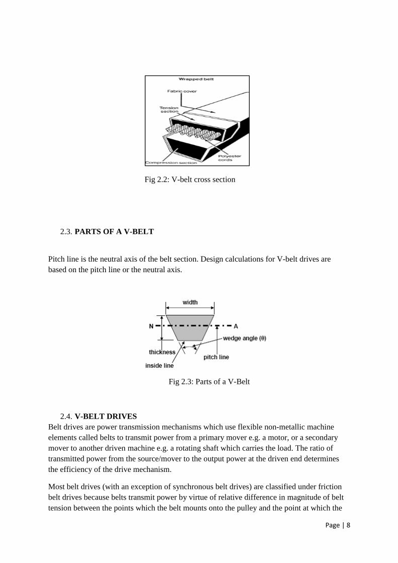
2.2. STRUCTURE OF A V-BELT
V-belts are ordinarily made of reinforced rubber and may be fabric wrapped to reduce
abrasion. Materials used consist of;
Fabric.
Nylon.
Cords of cotton, polyester, aramid, Kevlar etc.
All the above impregnated in a rubber matrix.
Page | 8
Fig 2.2: V-belt cross section
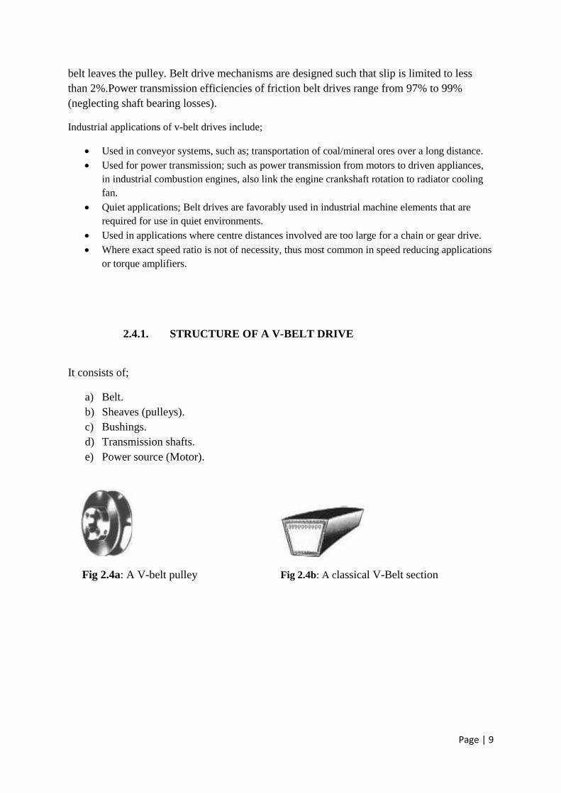
2.3. PARTS OF A V-BELT
Pitch line is the neutral axis of the belt section. Design calculations for V-belt drives are
based on the pitch line or the neutral axis.
Fig 2.3: Parts of a V-Belt
2.4. V-BELT DRIVES
Belt drives are power transmission mechanisms which use flexible non-metallic machine
elements called belts to transmit power from a primary mover e.g. a motor, or a secondary
mover to another driven machine e.g. a rotating shaft which carries the load. The ratio of
transmitted power from the source/mover to the output power at the driven end determines
the efficiency of the drive mechanism.
Most belt drives (with an exception of synchronous belt drives) are classified under friction
belt drives because belts transmit power by virtue of relative difference in magnitude of belt
tension between the points which the belt mounts onto the pulley and the point at which the
Page | 9
belt leaves the pulley. Belt drive mechanisms are designed such that slip is limited to less
than 2%.Power transmission efficiencies of friction belt drives range from 97% to 99%
(neglecting shaft bearing losses).
Industrial applications of v-belt drives include;
Used in conveyor systems, such as; transportation of coal/mineral ores over a long distance.
Used for power transmission; such as power transmission from motors to driven appliances,
in industrial combustion engines, also link the engine crankshaft rotation to radiator cooling
fan.
Quiet applications; Belt drives are favorably used in industrial machine elements that are
required for use in quiet environments.
Used in applications where centre distances involved are too large for a chain or gear drive.
Where exact speed ratio is not of necessity, thus most common in speed reducing applications
or torque amplifiers.
2.4.1. STRUCTURE OF A V-BELT DRIVE
It consists of;
a) Belt.
b) Sheaves (pulleys).
c) Bushings.
d) Transmission shafts.
e) Power source (Motor).
Fig 2.4a: A V-belt pulley Fig 2.4b: A classical V-Belt section
Page | 10
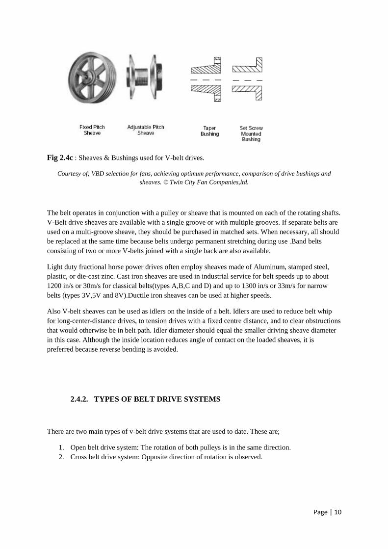
Fig 2.4c : Sheaves & Bushings used for V-belt drives.
Courtesy of; VBD selection for fans, achieving optimum performance, comparison of drive bushings and
sheaves. © Twin City Fan Companies,ltd.
The belt operates in conjunction with a pulley or sheave that is mounted on each of the rotating shafts.
V-Belt drive sheaves are available with a single groove or with multiple grooves. If separate belts are
used on a multi-groove sheave, they should be purchased in matched sets. When necessary, all should
be replaced at the same time because belts undergo permanent stretching during use .Band belts
consisting of two or more V-belts joined with a single back are also available.
Light duty fractional horse power drives often employ sheaves made of Aluminum, stamped steel,
plastic, or die-cast zinc. Cast iron sheaves are used in industrial service for belt speeds up to about
1200 in/s or 30m/s for classical belts(types A,B,C and D) and up to 1300 in/s or 33m/s for narrow
belts (types 3V,5V and 8V).Ductile iron sheaves can be used at higher speeds.
Also V-belt sheaves can be used as idlers on the inside of a belt. Idlers are used to reduce belt whip
for long-center-distance drives, to tension drives with a fixed centre distance, and to clear obstructions
that would otherwise be in belt path. Idler diameter should equal the smaller driving sheave diameter
in this case. Although the inside location reduces angle of contact on the loaded sheaves, it is
preferred because reverse bending is avoided.
2.4.2. TYPES OF BELT DRIVE SYSTEMS
There are two main types of v-belt drive systems that are used to date. These are;
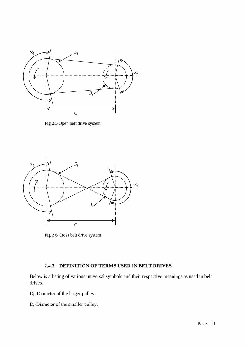
1. Open belt drive system: The rotation of both pulleys is in the same direction.
2. Cross belt drive system: Opposite direction of rotation is observed.
Page | 11
∝𝑙 𝐷𝑙
∝𝑠
𝐷𝑠
C
Fig 2.5 Open belt drive system
∝𝑙 𝐷𝑙
∝𝑠
𝐷𝑠
C
Fig 2.6 Cross belt drive system
2.4.3. DEFINITION OF TERMS USED IN BELT DRIVES
Below is a listing of various universal symbols and their respective meanings as used in belt
drives.
DL-Diameter of the larger pulley.
Ds-Diameter of the smaller pulley.
Page | 12
C- Center distance between the two pulleys.
∝𝑙 -Angle of wrap of the larger pulley.
∝𝑠 -Angle of wrap of the smaller pulley.
L=Pitch length of belt.
𝐺= Speed ratio of the drive.
2.4.4 THEORY OF BELT DRIVES
This refers to an in depth look at the various dimensional properties that can be used to describe a
belt/belt drive system. They include quantities such as; Belt length, diameters of large and small
pulley, angle of wrap, friction coefficients, centrifugal force, belt tension, torque and power
transmitted.
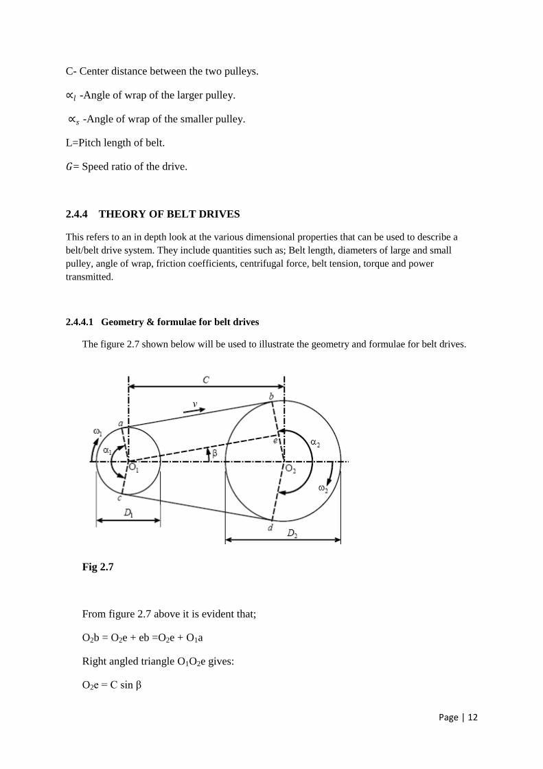
2.4.4.1 Geometry & formulae for belt drives
The figure 2.7 shown below will be used to illustrate the geometry and formulae for belt drives.
Fig 2.7
From figure 2.7 above it is evident that;
O2b = O2e + eb =O2e + O1a
Right angled triangle O1O2e gives:
O2e = C sin β
Page | 13
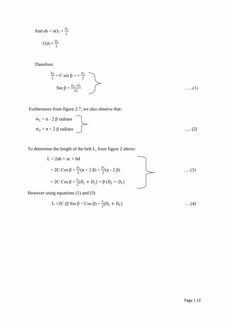
And eb = aO1 = 𝐷1
2
O2b = 𝐷2
2
Therefore:
𝐷2
2 = C sin β + =
𝐷1
2
Sin β = 𝐷2−𝐷1
2𝐶 …..(1)
Furthermore from figure 2.7, we also observe that:
∝1 = π - 2 β radians
∝2 = π + 2 β radians ..... (2)
To determine the length of the belt L, from figure 2 above:
L = 2ab + ac + bd
= 2C Cos β + 𝐷2
2(π + 2 β) +
𝐷1
2(π - 2 β) …. (3)
= 2C Cos β + 𝜋
2(𝐷1 + 𝐷2) + β (𝐷2 − 𝐷1)
However using equations (1) and (3)
L =2C (β Sin β + Cos β) + 𝜋
2(𝐷1 + 𝐷2) ….(4)

Page | 14
CHAPTER THREE
3. REVIEW OF LITERATURE ON DEVELOPMENT OF A COMPUTER
AIDED DESIGN FOR V-BELTS / V-BELT DRIVES
3.1. INTRODUCTION
Manufacturers have standardized and classified V-belts according to standard belt section
designated by alphabetical letters that are A, B, C, D, and E for various sizes in inch
dimensions while metric sizes are designated in numbers.
Each belt section has a standard measure of width, thickness, minimum sheave diameter for
use and kilo-watt range for use of the belts. These data are then tabulated for all V-belt
sections as shown in table 3.7.
3.2. DESIGN PROCESS
The design of V-belts follows a series of steps that guide the designer to the most suitable and
available standard belt section for use. The following is a detailed procedure followed in the
design of V-belts.
STEP1: Identify the Motor power used
Belt drives are used to transmit power from a primary mover such as a motor to an output
point such as a rotating shaft that carries a load. When designing a v-belt to use, it is
necessary to know how much power is given at the input since different belt sections have
limits to how much power they can transmit per belt .e.g. V-belt section-A belts can transmit
power in the range of 0.2kW – 7.5 kW while section-B belts transmit power from 0.7kw –
18.5 kW range.
STEP 2: Select a suitable service factor
Service factor is a modifier quantity used to multiply the power transmitted/input to give a
design power that will be used as the running power for the design. Service factor are
tabulated in terms of conditions of driven machinery, whether uniform, light shock, medium
shock, or heavy shock. Table 3.5 shows the various available service factors to use.
STEP 3: Determine the Design Power
Design power = (power transmitted x service factor)
STEP 4: Compare Tabulated Power for Belt section to Design Power
For example if the tabulated power for belt section A is 0.2 - 7.5kw range and the design
power from step above lies within this range, then a belt from section A is acceptable for use
otherwise if the design power exceeds the range ,then compare values in the next belt section
.i.e. B,C,D or E .

Page | 15
STEP 5: Matching Minimum Sheave Diameter
Belt sections are classified with corresponding minimum sheave diameter sizes for use. Sizes
could be in metric / imperial units. For example; from table 3.6 in the appendix section A
page 60, A belt of section-A is used with minimum sheave diameters from 75mm to 135mm.
STEP 6: Determine the speed ratio of the drive
Speed ratio, G = 𝑀𝑜𝑡𝑜𝑟 𝑠𝑝𝑒𝑒𝑑 (𝑟𝑝𝑚 )
𝑠𝑎𝑓𝑡 𝑠𝑝𝑒𝑒𝑑 (𝑟𝑝𝑚 )
Also G=𝐷1
𝐷2=
𝜔2
𝜔1
STEP 7: Determine the driven wheel sheave diameter, 𝑫𝟐:
𝐷2= G x 𝐷1
The calculated diameter of driven sheave obtained as shown above is then approximated to
the nearest standard size of sheave diameter available.
STEP 8: Belt speed, V (m/s):
Belt speed, V = 𝜋𝐷1𝑁1
60
Where; 𝐷1= Diameter of driving wheel sheave (m)
𝑁1 = Speed of motor/driving wheel (rev/min)
Suitable v-belt speeds lie between 20m/s to 25m/s. However speeds higher than 25m/s or
lower than 5m/s could result in failures.
STEP 9: Determine centre distance, C
This refers to the distance between the centre of the small sheave 𝐷1 to the center of the large
sheave 𝐷2.Center distance is limited by available space for use but is also advisable to lie
between 𝐷2 < C < 3(𝐷2 + 𝐷1).
STEP 10: Determining the Belt Length, 𝑳𝒑
𝐿𝑝=2C + 𝜋
2(𝐷2+𝐷1) +
(𝐷2−𝐷1)2
4𝐶
Where;
C=Center distance.
𝐷2 =Diameter of large sheave.
𝐷1 =Diameter of small sheave (driving).

Page | 16
The calculated length is then compared to nearest available standard belt length. Table 3.2 in
appendix section-A page 60, shows belt sections with corresponding inside circumferences,
while table 3.3 in page 60 also shows the length conversion dimensions5.
STEP 11: Determine the Belt Angles of wrap &
∝1 = π - 2 β radians
∝2 = π + 2 β radians
STEP 12: Angle of contact correction factor K1
Belt length correction factor K2
Use the belt speed and sheave diameter to determine the belt power rating for use.
STEP 13: Allowable power per belt, Ha
Ha = K1 x K2 x (Power rating per belt).
STEP 14: Number of belts for use
𝑁𝑝= 𝑑𝑒𝑠𝑖𝑔𝑛 𝑝𝑜𝑤𝑒𝑟
𝑚𝑜𝑑𝑖𝑓𝑖𝑒𝑑 𝑝𝑜𝑤𝑒𝑟 𝑟𝑎𝑡𝑖𝑛𝑔
In case of fractions, the next higher integer is used.
5 Shigley`s Mechanical Engineering design,8
th edition, by Richard G.Budynas,J.Keith Nisbett,page 879 table 17-
11
Page | 17
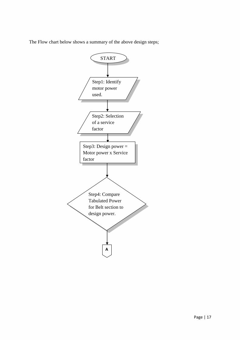
The Flow chart below shows a summary of the above design steps;
START
Step1: Identify
motor power
used.
Step2: Selection
of a service
factor
Step3: Design power =
Motor power x Service
factor
Step4: Compare
Tabulated Power
for Belt section to
design power.
A
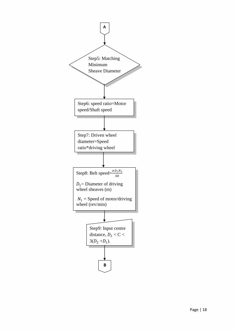
Page | 18
Step5: Matching
Minimum
Sheave Diameter
Step6: speed ratio=Motor
speed/Shaft speed
Step7: Driven wheel
diameter=Speed
ratio*driving wheel
diameter, D1
Step8: Belt speed=𝜋𝐷1𝑁1
60
𝐷1= Diameter of driving
wheel sheaves (m)
𝑁1 = Speed of motor/driving
wheel (rev/min)
Step9: Input centre
distance, 𝐷2 < C <
3(𝐷2 +𝐷1).
B
A
Page | 19
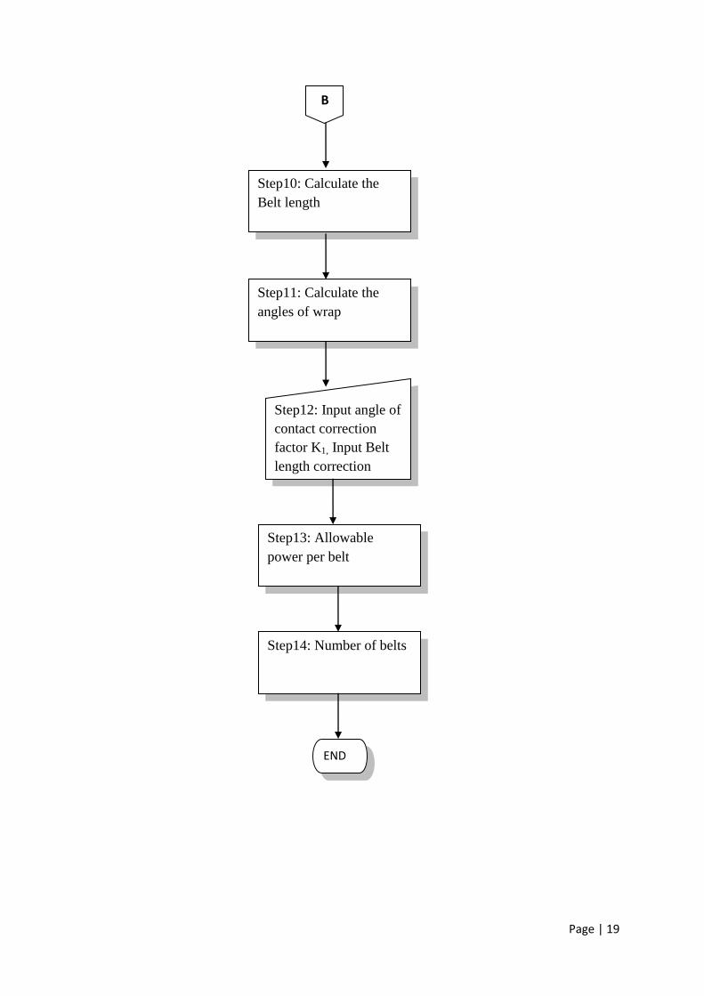
B
Step10: Calculate the
Belt length
Step11: Calculate the
angles of wrap
Step12: Input angle of
contact correction
factor K1, Input Belt
length correction
factor K2
Step13: Allowable
power per belt
Step14: Number of belts
END

Page | 20
3.3. COMPUTER AIDED DESIGN OF V-BELTS
C.A.D involves the use of computer programs/software’s which are programmed with inbuilt
commands similar to the theoretical calculations and steps involved in the design of v-belts
.The C.A.D program is made from a programming language in which algorithms are used to
create a systematic flow of steps/commands to be used in the final C.A.D software
developed.
In this case Programming language MATLAB was used. Matlab and other mathematical
computation tools are computer programs that combine computation and visualization power
that make them particularly useful tools for engineers. Furthermore it is both a computer
programming language and a software environment for using that language effectively.
The name Matlab stands for Matrix Laboratory, because the system was designed to make
matrix computations particularly easy. The Matlab environment allows the user to manage
variables, import and export data, perform calculations, generate plots, and develop and
manage files for use with Matlab.
The Matlab environment can also be described as an interactive environment as:
1. Single-line commands can be entered and executed, the results displayed and
observed, and then a second command can be executed that interacts with results
from the first command that remain in memory. This means that you can type
commands at the Matlab prompt and get answers immediately, which is very useful
for simple problems.
2. Matlab is an executable program, developed in a high-level language, which
interprets user commands.
3. Portions of the Matlab program execute in response to the user input, results are
displayed, and the program waits for additional user input.
4. When a command is entered that doesn’t meet the command rules, an error message
is displayed. The corrected command can then be entered.
5. While this interactive, line-by-line execution of Matlab commands is convenient for
simple computational tasks, a process of preparation and execution of programs
called scripts is employed for more complicated computational tasks.
A script is list of Matlab commands, prepared within a text editor. Matlab then executes a
script by reading a command from the script file, executing it, and then repeating the process
on the next command in the script file.
Errors in the syntax of a command are detected when Matlab attempts to execute the
command. A syntax error message is displayed and execution of the script is halted.
When syntax errors are encountered, the user must edit the script file to correct the error and
then direct Matlab to execute the script again.
Page | 21
The script may execute without syntax errors, but produce incorrect results when a logic error
has been made in writing the script, which also requires that the script be edited and
execution re-initiated.
3.3.1. How to create a C.A.D from Matlab program
Engineering often involves applying a consistent, structured approach to the solving of
problems. A general problem-solving approach and method can be defined, although
variations will be required for specific problems.
Problems must be approached methodically, applying an algorithm, or step-by-step procedure
by which one arrives at a solution.
The problem-solving process for a computational problem can be outlined as follows:
a) Define the problem.
b) Create a mathematical model.
c) Develop a computational method for solving the problem.
d) Implement the computational method.
e) Test and assess the solution.
The boundaries between these steps can be blurred and for specific problems one or two of
the steps may be more important than others.
A) Problem Definition:
The first steps in problem solving include:
• Recognize and define the problem precisely by exploring and understanding it
thoroughly.
• Determine what question is to be answered and what output or results are to be
produced?
• Determine what theoretical and experimental knowledge can be applied?
• Determine what input information or data is available?
After defining the problem then:
• Collect all data and information about the problem.
• Verify the accuracy of this data and information.
• Determine what information you must find: intermediate results or data may need to
be found before the required answer or results can be found.
B) Mathematical Model:
To create a mathematical model of the problem to be solved:
• Determine what fundamental principles are applicable.
• Draw sketches or block diagrams to better understand the problem.
• Define necessary variables and assign notation.

Page | 22
• Reduce the problem as originally stated into one expressed in purely mathematical
terms.
• Apply mathematical expertise to extract the essentials from the underlying physical
description of the problem.
• Simplify the problem only enough to allow the required information and results to be
obtained.
• Identify and justify the assumptions and constraints inherent in this model.
C) Computational Method:
A computational method for solving the problem is to be developed, based on the
mathematical model.
• Derive a set of equations that allow the calculation of the desired parameters and
variables.
• Develop an algorithm, or step-by-step method of evaluating the equations involved in
the solution.
• Describe the algorithm in mathematical terms and then implement as a computer
program.
D) Implementation of Computational Method:
Once a computational method has been identified, the next step is to carry out the method
with a computer, whether human or silicon.
Some things to consider in this implementation:
• Assess the computational power needed, as an acceptable implementation may be
hand calculation with a pocket calculator.
• If a computer program is required, a variety of programming languages, each with
different properties, are available.
• The ability to choose the proper combination of programming language and computer,
and use them to create and execute a correct and efficient implementation of the
method, requires both knowledge and experience.
The mathematical algorithm developed in the previous step must be translated into a
computational algorithm and then implemented as a computer program.
The steps in the algorithm should first be outlined and then decomposed into smaller steps
that can be translated into programming commands.
One of the strengths of Matlab is that its commands match very closely to the steps that are
used to solve engineering problems; thus the process of determining the steps to solve the
problem also determines the Matlab commands. Furthermore, Matlab includes an extensive
toolbox of numerical analysis algorithms, so the programming effort often involves
implementing the mathematical model, characterizing the input data, and applying the
available numerical algorithms.

Page | 23
E) Test and Assess the Solution:
The final step is to test and assess the solution. In many aspects, assessment is the most open-
ended and difficult of the five steps involved in solving computational problems.
The numerical solution must be checked carefully:
• A simple version of the problem should be hand checked.
• Solution is either known or which can be obtained by independent means, such as
hand or calculator computation.
• Intermediate values should be compared with expected results and estimated
variations.
• When values deviate from expected results more than was estimated, the source of the
deviation should be determined and the program modified as needed.
• A “reality check” should be performed on the solution to determine if it makes sense.
3.3.1.1. Algorithms used in Matlab
In order to understand how to use Matlab /even other programming languages it is necessary
to have an understanding on fundamental programming terms.
Below is a list of definitions of computing terms:
Command: This is a user-written statement in a computer language that provides
instructions to the computer.
Variable: The name given to a quantity that can assume a value.
Default: The action taken or value chosen if none has been specified.
Arguments: The values provided as inputs to a command.
Returns: The results provided by the computer in response to a command.
Execute: To run a program or carry out the instructions specified in a command.
Display: Provide a listing of text information on the computer monitor or screen.
In Matlab, variable names can be assigned to represent numerical values but first the rules to
be used for these variable names are:
The names must start with a letter.
They may consist of the letters a-z, digits 0-9, and underscore character (_).
May be as long as preferred but Matlab only recognizes the first 31 characters.
Note also that it should be case sensitive: Area, AREa, AREA...e.t.c are all different
variable names.
Syntax/Assignment statement used in Matlab commands are of the form:
Variable=number
Variable=expression
Page | 24
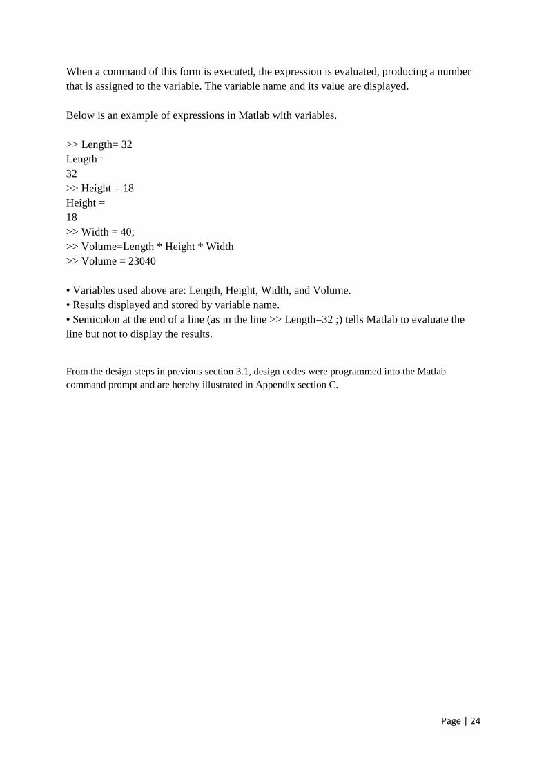
When a command of this form is executed, the expression is evaluated, producing a number
that is assigned to the variable. The variable name and its value are displayed.
Below is an example of expressions in Matlab with variables.
>> Length= 32
Length=
32
>> Height = 18
Height =
18
>> Width = 40;
>> Volume=Length * Height * Width
>> Volume = 23040
• Variables used above are: Length, Height, Width, and Volume.
• Results displayed and stored by variable name.
• Semicolon at the end of a line (as in the line >> Length=32 ;) tells Matlab to evaluate the
line but not to display the results.
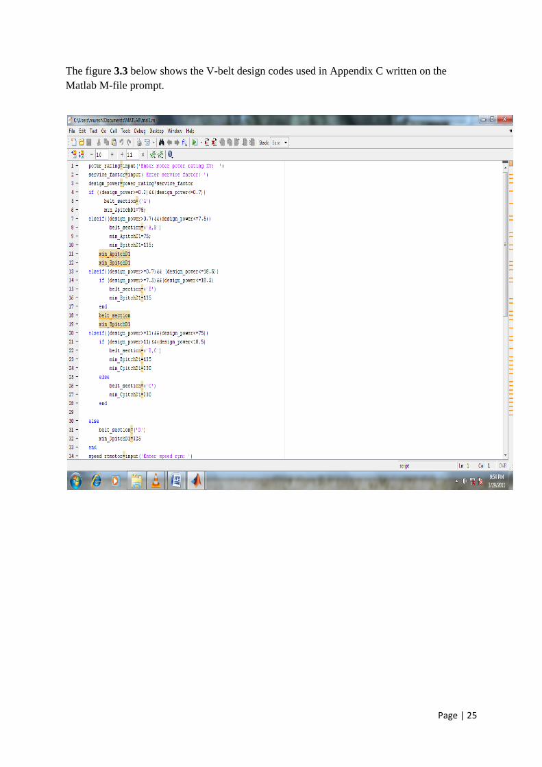
From the design steps in previous section 3.1, design codes were programmed into the Matlab
command prompt and are hereby illustrated in Appendix section C.
Page | 25
The figure 3.3 below shows the V-belt design codes used in Appendix C written on the
Matlab M-file prompt.
Page | 26
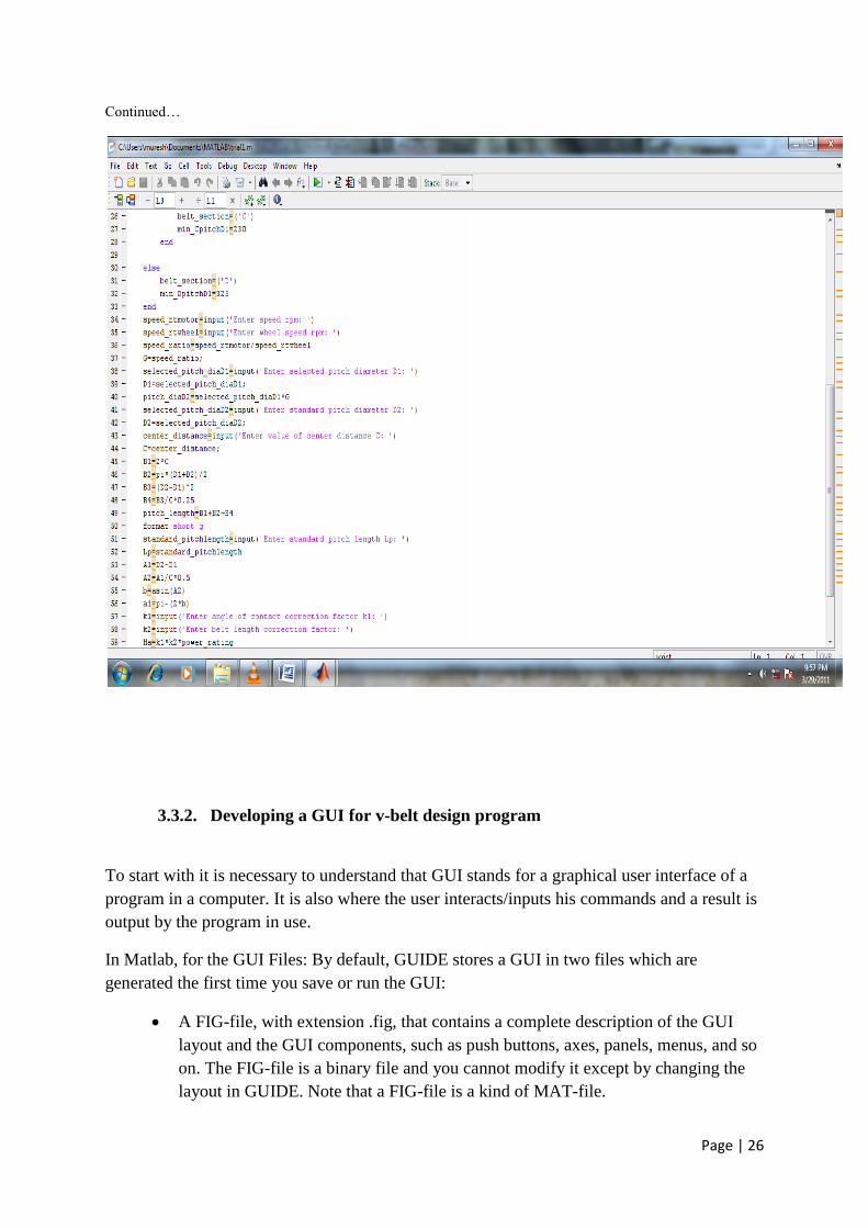
Continued…
3.3.2. Developing a GUI for v-belt design program
To start with it is necessary to understand that GUI stands for a graphical user interface of a
program in a computer. It is also where the user interacts/inputs his commands and a result is
output by the program in use.
In Matlab, for the GUI Files: By default, GUIDE stores a GUI in two files which are
generated the first time you save or run the GUI:
A FIG-file, with extension .fig, that contains a complete description of the GUI
layout and the GUI components, such as push buttons, axes, panels, menus, and so
on. The FIG-file is a binary file and you cannot modify it except by changing the
layout in GUIDE. Note that a FIG-file is a kind of MAT-file.
Page | 27
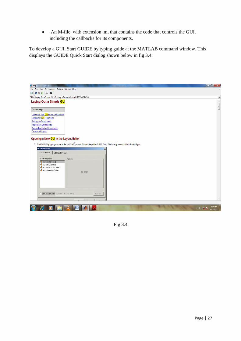
An M-file, with extension .m, that contains the code that controls the GUI,
including the callbacks for its components.
To develop a GUI, Start GUIDE by typing guide at the MATLAB command window. This
displays the GUIDE Quick Start dialog shown below in fig 3.4:
Fig 3.4

Page | 28
For opening a New GUI in the Layout Editor, Go to File New GUI. The dialogue box
below appears.
Fig 3.5
Page | 29
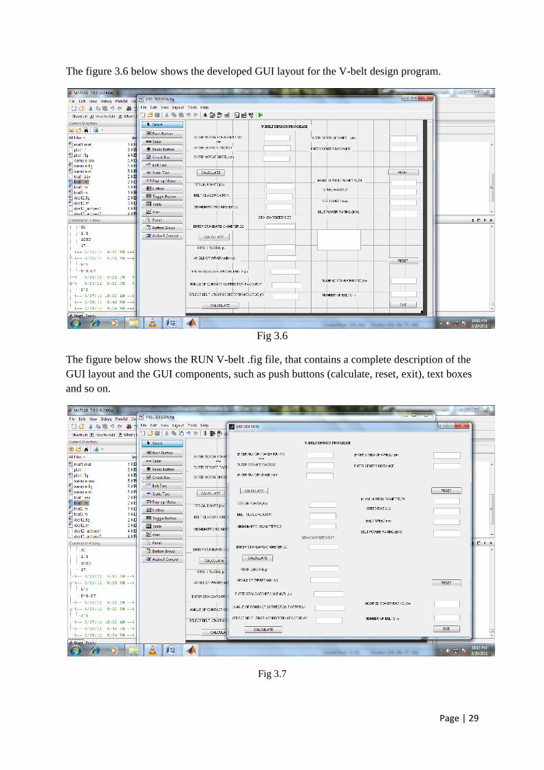
The figure 3.6 below shows the developed GUI layout for the V-belt design program.
Fig 3.6
The figure below shows the RUN V-belt .fig file, that contains a complete description of the
GUI layout and the GUI components, such as push buttons (calculate, reset, exit), text boxes
and so on.
Fig 3.7

Page | 30
CHAPTER FOUR
4. REVIEW OF LITERATURE ON CHAINS, CHAIN DRIVES AND
COMPUTER AIDED DESIGN OF CHAIN DRIVES
4.1. INTRODUCTION TO CHAINS
Chains may be regarded as a belt that is built up of short rigid links, which are hinged
together in order to provide the flexibility that is necessary for the chain to be wrapped
around the driving and driven wheels. These wheels have projected teeth, which fit into
suitable recesses in the chain links and thus enable a positive drive that operates without slip.
The wheels are known as chain sprockets and they bear a superficial resemblance to spur
wheels. However the tooth profiles on the chain sprockets are quite different from those of
spur gears.
Some principal advantages of chain drives as compared to belt drives are the following:
Chain drives may be used in applications with relatively long as well as short center
distances. The center distanced can be as large as eight meters.
Chain drives are compact as compared to flat belt drives.
Chain drives impose less severe loads on shafts as compared to belt drives.
Under ideal conditions, the mechanical efficiency may be as high as 98%to 99%.
There is no slippage between chain and sprocket teeth.
Chain stretch is negligible, allowing it to carry heavy loads.
Long shelf life because metal chain ordinarily doesn’t deteriorate with age and is
unaffected by sun, reasonable ranges of heat, moisture, and oil.
On the other hand, some disadvantages of chain drives as compared to belt drives are:
Chain drives are noisy in operation.
Chain drives are more sensitive to misalignment than belt drives.
Initial cost of chain is relatively high.
Due to wear in the chain joints, the chain stretches permanently with time thus
increasing the chain pitch with time.
Chain drives require lubrication, more servicing, maintenance and repairs as
compared to belt drives.
Chain drives find wide applications in industry. They are used with velocity ratios of less
than 8, linear chain speeds of up to 25m/s, power ratings of up to 110kw and sometimes
more. Chains can be classified into the following categories:
Power transmission chains.
Hoisting chains.

Page | 31
Traction or pulling chains.
Our main concern is with power transmission chains. The most common types of are bush
chains, roller chains, and inverted tooth chains. However the most commonly used power
transmission chain is the roller chain. In a roller chain the outer rows of link plates are known
as pin links or coupling links whereas the inner link plates are known as roller links. The pins
are press-fitted into the pin links and the bushes, through which the pins pass, are press-fitted
into the roller links. The chain rollers are mounted on the bushes so as to be able to rotate
freely within and relative to the bushes. The sprocket teeth are specially designed to engage
smoothly with the rollers.
Roller chains are normally made of case-hardened and ground alloy steel. Materials such as
brass and bronze are used in special applications such as in food processing machines or
where corrosion may be a problem.
Power transmission chains are designated by:
The pitch of the chain, which is the distance along a straight line joining the axes of
two adjacent chain joints.
The nominal width of the chain, which is the transverse distance between the inner
link plate.
The roller diameter, which is the outer diameter of the roller.
Roller chain is standardized in a range of pitches from 0.25 in. to 3 in. (6.35 mm to 76.2
mm); silent chain from 0.375 in. to 2 in. (9.525 mm to 50.8 mm). The strength and
horsepower capacity of a chain increase with pitch, but for high-speed drives, smaller pitch
must be used to limit sprocket size and variation in linear chain speed. Ideally, the smaller
sprocket should have an odd number of teeth, not less than 17 and preferably more. Usually
the speed ratio should not exceed 6:1, and the larger sprocket should not have more than 120
teeth. Sprockets can be very close together, but the chain should wrap around the smaller
sprocket at least 120 degrees. A centre distance of 30 to 50 pitches is good but 80 pitches is a
recommended maximum. The dimensions of various chain components are normally
determined in terms of chain pitch.
Page | 32
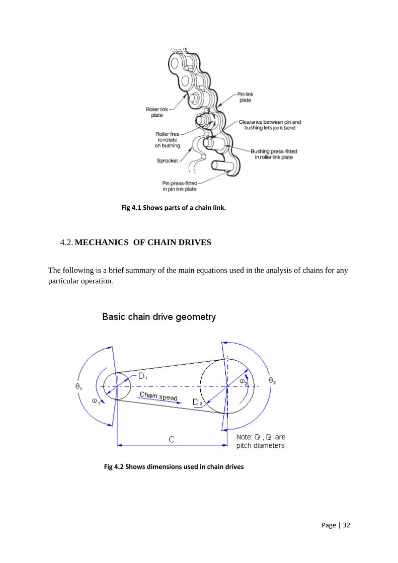
Fig 4.1 Shows parts of a chain link.
4.2. MECHANICS OF CHAIN DRIVES
The following is a brief summary of the main equations used in the analysis of chains for any
particular operation.
Fig 4.2 Shows dimensions used in chain drives
Page | 33
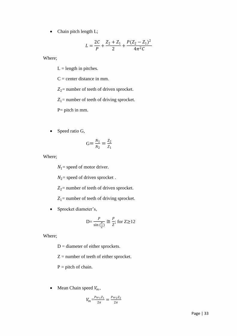
Chain pitch length L;
𝐿 =2𝐶
𝑃+𝑍2 + 𝑍1
2+𝑃(𝑍2 − 𝑍1)2
4𝜋2𝐶
Where;
L = length in pitches.
C = center distance in mm.
𝑍2= number of teeth of driven sprocket.
𝑍1= number of teeth of driving sprocket.
P= pitch in mm.
Speed ratio G,
G=𝑁1
𝑁2=
𝑍2
𝑍1
Where;
𝑁1= speed of motor driver.
𝑁2= speed of driven sprocket .
𝑍2= number of teeth of driven sprocket.
𝑍1= number of teeth of driving sprocket.
Sprocket diameter’s,
D= 𝑃
sin (𝜋
𝑍)≅
𝑃
𝑍; for Z≥12
Where;
D = diameter of either sprockets.
Z = number of teeth of either sprocket.
P = pitch of chain.
Mean Chain speed 𝑉𝑚 ,
𝑉𝑚=𝑃𝜔1𝑍1
2𝜋=
𝑃𝜔2𝑍2
2𝜋
Page | 34
Where;
𝜔1= angular speed of driving sprocket.
𝜔2= angular speed of driven sprocket.
𝑍2= number of teeth of driven sprocket.
𝑍1= number of teeth of driving sprocket.
4.3. DESIGN OF A ROLLER CHAIN DRIVE
A roller Chain by nature of its design is capable of transmitting high torque loads, and
provides the ideal drive media for the connection of slow to medium speed shafts located on
extended centers. The selection and application is reasonably simple by following normal
engineering practices, but there are points of good design practice specific to Roller Chain
Drives, and consideration of these will ensure successful drive design.
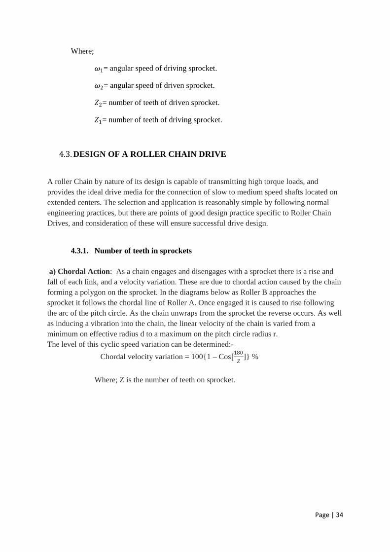
4.3.1. Number of teeth in sprockets
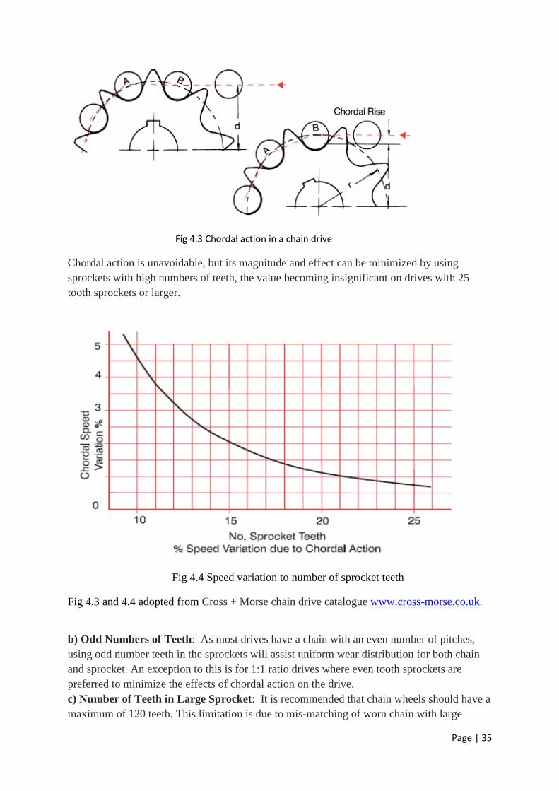
a) Chordal Action: As a chain engages and disengages with a sprocket there is a rise and
fall of each link, and a velocity variation. These are due to chordal action caused by the chain
forming a polygon on the sprocket. In the diagrams below as Roller B approaches the
sprocket it follows the chordal line of Roller A. Once engaged it is caused to rise following
the arc of the pitch circle. As the chain unwraps from the sprocket the reverse occurs. As well
as inducing a vibration into the chain, the linear velocity of the chain is varied from a
minimum on effective radius d to a maximum on the pitch circle radius r.
The level of this cyclic speed variation can be determined:-
Chordal velocity variation = 100{1 – Cos[180
𝑍]} %
Where; Z is the number of teeth on sprocket.
Page | 35
Fig 4.3 Chordal action in a chain drive
Chordal action is unavoidable, but its magnitude and effect can be minimized by using
sprockets with high numbers of teeth, the value becoming insignificant on drives with 25
tooth sprockets or larger.
Fig 4.4 Speed variation to number of sprocket teeth
Fig 4.3 and 4.4 adopted from Cross + Morse chain drive catalogue www.cross-morse.co.uk.
b) Odd Numbers of Teeth: As most drives have a chain with an even number of pitches,
using odd number teeth in the sprockets will assist uniform wear distribution for both chain
and sprocket. An exception to this is for 1:1 ratio drives where even tooth sprockets are
preferred to minimize the effects of chordal action on the drive.
c) Number of Teeth in Large Sprocket: It is recommended that chain wheels should have a
maximum of 120 teeth. This limitation is due to mis-matching of worn chain with large
Page | 36
sprockets which increases with the number of teeth in the sprocket. A simple formula to
indicate percentage of chain wear a sprocket can accommodate is 200%
𝑍 It is normally
considered good practice to replace chain if wear elongation exceeds 2%. It is considered
good practice that the sum of teeth on drives and driven sprocket should not be less than 50.
Where both the driver and driven sprockets are operated by the same chain, e.g. on a 1:1 ratio
drive, both sprockets should have 25 teeth each.
4.3.2. Drive Ratio
Roller Chain operates at high efficiency on drives with reduction ratios up to 3:1, but can be
used effectively for drives up to 6:1 reduction. Higher ratios are not recommended but on
some very slow speed drives reductions up to 10:1 have been used. High drive ratios require
sprockets with large number of teeth, which restrict maximum chain wear with a resultant
reduction in chain life. For reduction ratios above 5:1 consideration should be given to two-
stage drive with idler shaft.
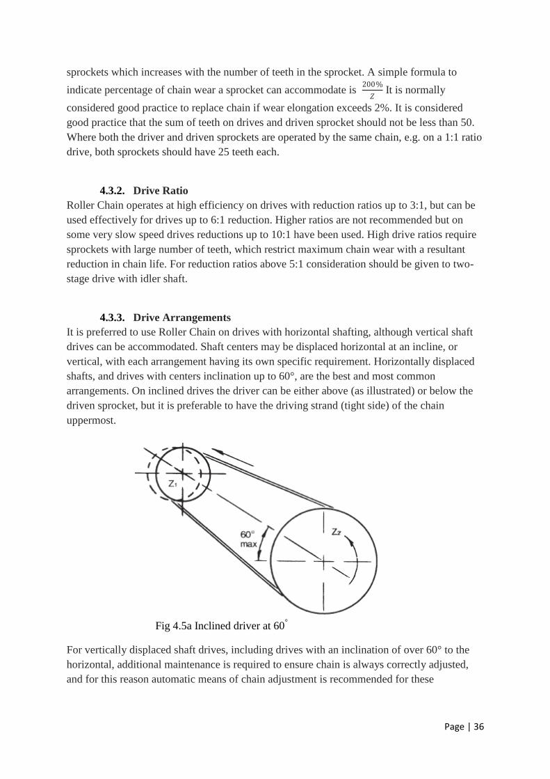
4.3.3. Drive Arrangements
It is preferred to use Roller Chain on drives with horizontal shafting, although vertical shaft
drives can be accommodated. Shaft centers may be displaced horizontal at an incline, or
vertical, with each arrangement having its own specific requirement. Horizontally displaced
shafts, and drives with centers inclination up to 60°, are the best and most common
arrangements. On inclined drives the driver can be either above (as illustrated) or below the
driven sprocket, but it is preferable to have the driving strand (tight side) of the chain
uppermost.
Fig 4.5a Inclined driver at 60
°
For vertically displaced shaft drives, including drives with an inclination of over 60° to the
horizontal, additional maintenance is required to ensure chain is always correctly adjusted,
and for this reason automatic means of chain adjustment is recommended for these

Page | 37
arrangements. It is always preferred to have the driver sprocket above the driven sprocket, as
chain wear creates reduced contact on the lower sprocket.
Fig 4.5b Shows vertically displaced shaft drives
Roller Chain is not recommended for drives with vertical shafts, but providing the drive is
well engineered, and certain basic rules followed, a satisfactory drive can be achieved. As the
chain is supported by its side-plates on the sprockets, it is essential to use sprockets with high
numbers of teeth (minimum 25 teeth) to spread the load. To minimize side loads on the chain
shaft, centers should be kept to a minimum (30 pitches max), and multistrand chains used
where possible. For slow speed drives (up to 1 M/S) special chain guides are available to
support simplex chain for longer centre drives. It is imperative that chains are maintained in
correct tension at all times, if acceptable life is to be achieved, and to minimize the effects of
wear, chain selection should be made with an additional design factor of 2.
4.3.4 Shafts Centre Distance
In general the preferred range for center distance for roller chain drives that allow adjustable
center distance is 30 to 50 times chain pitch. Drives with centers up to 80 times pitch will
perform satisfactorily providing adequate adjustment of chain tension is available. For very
long centers, consideration should be given using two stage drive with idler, or alternatively
for lightly loaded, slow speed (up to 1 m/s) drives, supporting both strands of chain on chain
guides.
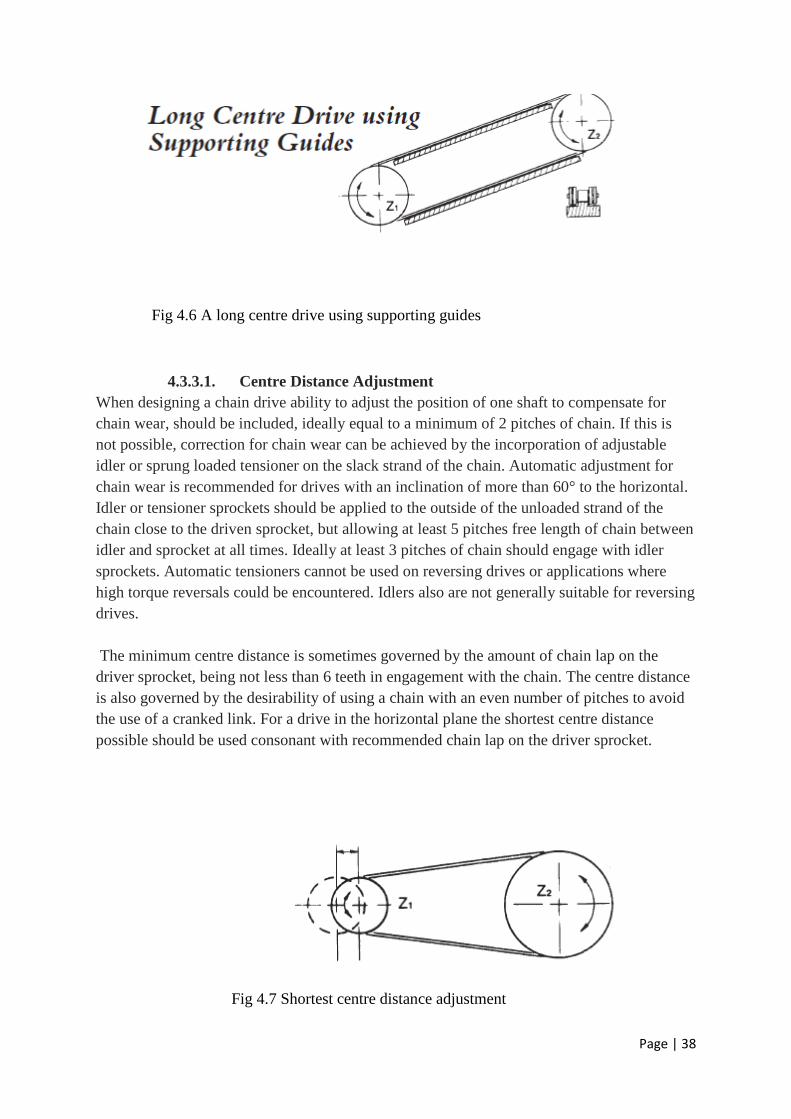
Page | 38
Fig 4.6 A long centre drive using supporting guides
4.3.3.1. Centre Distance Adjustment
When designing a chain drive ability to adjust the position of one shaft to compensate for
chain wear, should be included, ideally equal to a minimum of 2 pitches of chain. If this is
not possible, correction for chain wear can be achieved by the incorporation of adjustable
idler or sprung loaded tensioner on the slack strand of the chain. Automatic adjustment for
chain wear is recommended for drives with an inclination of more than 60° to the horizontal.
Idler or tensioner sprockets should be applied to the outside of the unloaded strand of the
chain close to the driven sprocket, but allowing at least 5 pitches free length of chain between
idler and sprocket at all times. Ideally at least 3 pitches of chain should engage with idler
sprockets. Automatic tensioners cannot be used on reversing drives or applications where
high torque reversals could be encountered. Idlers also are not generally suitable for reversing
drives.
The minimum centre distance is sometimes governed by the amount of chain lap on the
driver sprocket, being not less than 6 teeth in engagement with the chain. The centre distance
is also governed by the desirability of using a chain with an even number of pitches to avoid
the use of a cranked link. For a drive in the horizontal plane the shortest centre distance
possible should be used consonant with recommended chain lap on the driver sprocket.
Fig 4.7 Shortest centre distance adjustment

Page | 39
Fig 4.8 an idler or tensioner sprocket in use.
Fig 4.5, 4.6, 4.7 and 4.8 courtesy of Cross + Morse chain drive catalogue www.cross-
morse.co.uk
4.3.3.2. Chain lubrication
An adequate supply of lubrication is necessary to ensure a satisfactory wear life for any chain
drive. Roller chain when supplied is coated in a heavy petroleum grease to provide protection
until installation. For some slow, light load applications this lubrication is adequate providing
a short wear life can be accepted, but for the majority of applications an oil lubrication
system to provide further lubrication will be required, the type being dependant on chain size,
loads and operating speed. When oil is applied to a roller chain a separating wedge of fluid is
formed in the operating joints, similar to journal bearings, thereby minimizing metal to metal
contact. When applied in sufficient volume the oil also provides effective cooling and impact
dampening at higher speeds. Chain life will vary appreciably depending on the lubrication
system used, and therefore it is important that lubrication recommendations are complied
with. The chain rating tables used for selection only apply for drives lubricated in line with
the following recommendations. Chain drives should be encased for protection from dirt and
moisture, and oil supplies should be kept free of contamination. A good quality, petroleum-
based, non detergent thin oil should be used, and changed periodically (Max. 3000 hours
operating life). Heavy oils and greases are not recommended for most applications, because
they are too stiff to enter the small spaces between precision chain components.
There are four basic types of lubrication for chain drives, the correct one being determined by
chain size and speed;
a) Manual Lubrication
Oil is applied with a brush or oil-can at least once every 8 hours of operation. The volume
and frequency of application should be sufficient to keep the chain wet with oil and prevent
overheating or discoloration of lubricant in the chain joints. The use of aerosol-can lubricant
is often satisfactory on slow speed drives. It is important that the lubricant used is of a type
specified for roller chains.
Page | 40
b) Drip Feed Lubrication
Oil drops are directed between the link plate edges from a drip lubricator. Volume and
frequency should be sufficient to prevent discoloration of lubricant in the chain joints.
Precaution must be taken against misdirection of the drops by wind from the passing chain.
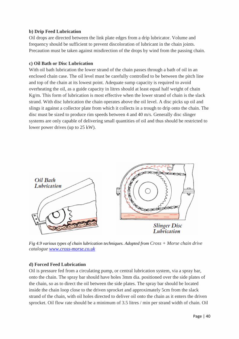
c) Oil Bath or Disc Lubrication
With oil bath lubrication the lower strand of the chain passes through a bath of oil in an
enclosed chain case. The oil level must be carefully controlled to be between the pitch line
and top of the chain at its lowest point. Adequate sump capacity is required to avoid
overheating the oil, as a guide capacity in litres should at least equal half weight of chain
Kg/m. This form of lubrication is most effective when the lower strand of chain is the slack
strand. With disc lubrication the chain operates above the oil level. A disc picks up oil and
slings it against a collector plate from which it collects in a trough to drip onto the chain. The
disc must be sized to produce rim speeds between 4 and 40 m/s. Generally disc slinger
systems are only capable of delivering small quantities of oil and thus should be restricted to
lower power drives (up to 25 kW).
Fig 4.9 various types of chain lubrication techniques. Adopted from Cross + Morse chain drive
catalogue www.cross-morse.co.uk
d) Forced Feed Lubrication
Oil is pressure fed from a circulating pump, or central lubrication system, via a spray bar,
onto the chain. The spray bar should have holes 3mm dia. positioned over the side plates of
the chain, so as to direct the oil between the side plates. The spray bar should be located
inside the chain loop close to the driven sprocket and approximately 5cm from the slack
strand of the chain, with oil holes directed to deliver oil onto the chain as it enters the driven
sprocket. Oil flow rate should be a minimum of 3.5 litres / min per strand width of chain. Oil

Page | 41
reservoir capacities should be a minimum of 3 times oil flow rate, and lubrication system
should include a full flow oil filter.
4.4. SELECTION PROCEDURE FOR CHAIN DRIVES WITH TWO
SPROCKETS
In order to use a selection procedure, it is first necessary to assemble all data relevant to the
application, which should include:
a) Power to be transmitted.
b) Input shaft speed, and output speed required or drive ratio.
c) Type of driver and driven equipment (uniform load, moderate shock, heavy
shock).
d) Center distance between shafts.
e) Environmental conditions.
f) Limits on space and position of drive.
g) Proposed lubrication method.
STEP 1: Service Factor - 𝒇𝟏
The service factor f1 can be determined from details of the driver and driven equipment by
selection from the table below. The service factor is applied to take into consideration the
source of power, nature of the load, load inertia strain or shock, and the average hours per day
of service. Normal duty drives are those with relatively little shock or load variation.
STEP 2: Calculation of drive ratio
The sprocket sizes are determined by the drive ratio required.
Drive Ratio = 𝑅𝑃𝑀 𝑜𝑓 𝑖𝑔 𝑠𝑝𝑒𝑒𝑑 𝑠𝑎𝑓𝑡 𝑁1
𝑅𝑃𝑀 𝑜𝑓 𝑙𝑜𝑤 𝑠𝑝𝑒𝑒𝑑 𝑠𝑎𝑓𝑡 𝑁2
=𝑁𝑜 .𝑜𝑓 𝑡𝑒𝑒𝑡 𝑜𝑓 𝑙𝑎𝑟𝑔𝑒 𝑠𝑝𝑟𝑜𝑐𝑘𝑒𝑡 𝑍2
𝑁𝑜 .𝑜𝑓 𝑡𝑒𝑒𝑡 𝑜𝑓 𝑠𝑚𝑎𝑙𝑙 𝑠𝑝𝑟𝑜𝑐𝑘𝑒𝑡 𝑍1
Unless shaft speeds are very low it is advisable to use a minimum of 17 tooth sprockets. If the
drive operates at high speeds or is subject to impulse load sprockets should have at least 25
teeth and should be hardened. For low ratio drives, sprockets with high numbers of teeth
minimize joint articulation, and bearing loads, thus extending chain life. On drives where
ratios exceed 5:1 the designer should consider using compound drives for maximum service
life.
STEP 3: Calculate the design power
Having determined values for service factor, the design Power can be determined.
𝑃𝑑= 𝑃 × 𝑓1
Page | 42
By relating the design Power 𝑃𝑑 with the rotational speed of the small sprocket 𝑁1 the correct
size of chain for the application can be selected from standard charts.
STEP 4: Select drive chain
From the rating chart, the smallest pitch of simplex chain is selected to transmit the design
power at the speed of the driving sprocket 𝑍1. This normally results in the most economical
drive selection. If the design power is now greater than that shown for the simplex chain, then
consider a multiplex chain of the same pitch size as detailed in the ratings chart.
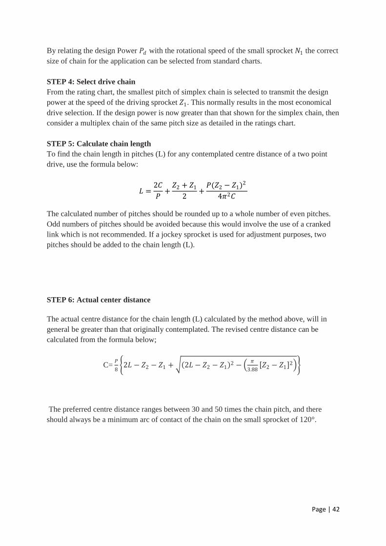
STEP 5: Calculate chain length
To find the chain length in pitches (L) for any contemplated centre distance of a two point
drive, use the formula below:
𝐿 =2𝐶
𝑃+𝑍2 + 𝑍1
2+𝑃(𝑍2 − 𝑍1)2
4𝜋2𝐶
The calculated number of pitches should be rounded up to a whole number of even pitches.
Odd numbers of pitches should be avoided because this would involve the use of a cranked
link which is not recommended. If a jockey sprocket is used for adjustment purposes, two
pitches should be added to the chain length (L).
STEP 6: Actual center distance
The actual centre distance for the chain length (L) calculated by the method above, will in
general be greater than that originally contemplated. The revised centre distance can be
calculated from the formula below;
C= 𝑃
8 2𝐿 − 𝑍2 − 𝑍1 + 2𝐿 − 𝑍2 − 𝑍1 2 −
𝜋
3.88 𝑍2 − 𝑍1 2
The preferred centre distance ranges between 30 and 50 times the chain pitch, and there
should always be a minimum arc of contact of the chain on the small sprocket of 120°.
Page | 43
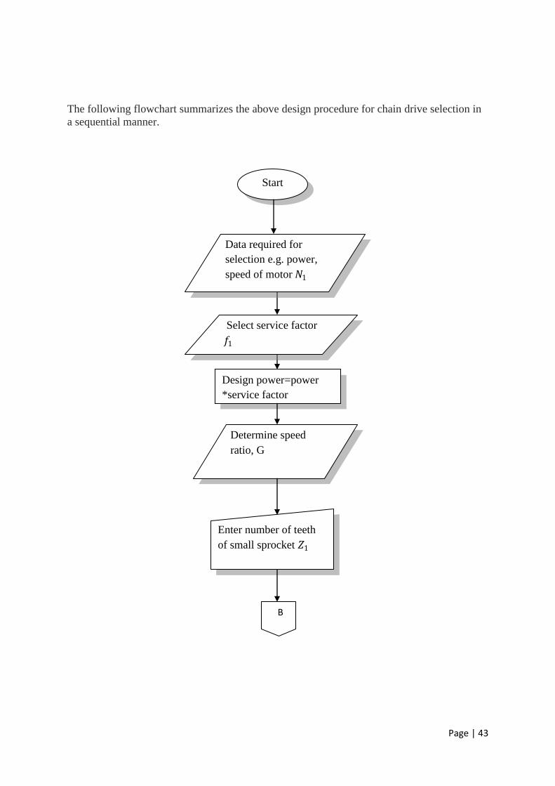
The following flowchart summarizes the above design procedure for chain drive selection in
a sequential manner.
Start
Data required for
selection e.g. power,
speed of motor 𝑁1
Select service factor
𝑓1
Design power=power
*service factor
Determine speed
ratio, G
Enter number of teeth
of small sprocket 𝑍1
B

Page | 44
Determine number of teeth of large
sprocket 𝑍2 from speed ratio G
Determination of
appropriate pitch
size
Enter center distance C
Calculate chain pitch length
𝐿𝑝 in number of pitches
Determine type of
lubrication.
END
B
Page | 45
4.5. COMPUTER AIDED DESIGN OF CHAIN DRIVES
This work presents a computer-aided analysis for the selection of roller chain drives, which
are commonly used in mechanical power transmission systems. Computer programs are
written and proposed to improve the traditional method of drive selection for the roller chain
drives. The algorithms are mainly based on the existing equations for the mechanics of the
drives, including the geometry and the power transmission capabilities. The purpose of
attempting to computerize the selection procedures is to reduce the number of tables and
charts that are required in traditional selection routines. In addition, it is also intended to cut
down the amount of iteration, time and calculation work performed.
In this case MATLAB software was used in the creation of this program. This is because
MATLAB is a high-performance language for technical computing and integrates
computation, visualization, and programming in an easy-to-use environment where problems
and solutions are expressed in familiar mathematical notation.
In analysis of chain drives, link plate fatigue equation governs failure of link at lower speeds
whereas roller and bushing fatigue tend to govern failure at higher speeds. In developing this
program the limiting horsepower used in the design is the link plate fatigue equation which is
summarized as follows;
𝐻𝑑 = 0.004𝑁1.08𝑛0.9𝑃 3−0.07𝑃
Where;
𝐻𝑑 =Design horse power
N = motor speed in RPM
n=number of teeth of driving sprocket
P= chain pitch
Since the program is based on the user selecting the pitch required for any application the
above equation was rearranged such that the pitch was made the subject of the formula.
Therefore;
𝑃 3−0.07𝑃 = 𝐻𝑑
0.004𝑁1.08𝑛0.09
The appropriate value of pitch is determined when the value entered on the left hand side of
the equation is greater than or equal to the value on the right hand side. Variables used
include motor rating, center distance, service factor, number of teeth of small sprocket, speed
of rotating component and pitch. The following is the algorithm used to develop the program
for chain design.

Page | 46
4.5.1. Developing a graphical user interface (GUI)
With the desired algorithm in place, the above program is presented in a user friendly manner
by developing a graphical user interface. MATLAB has presented a sequential procedure that
makes it easy to create the desired GUI. The following pictures show the procedure used in
the creation of the GUI for chain drives. From the file menu, select new, then go down to
GUI.
Fig 4.5.1

Page | 47
On clicking, the GUI quick start guide dialogue box appears.
Fig 4.5.2
By clicking the blank GUI (default) option the following figure appears. It is here that the
desired outlook of the program is created.
Fig 4.5.3
Page | 48
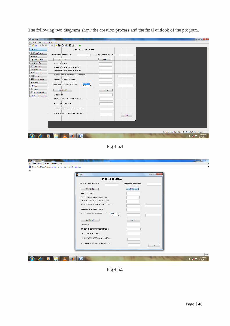
The following two diagrams show the creation process and the final outlook of the program.
Fig 4.5.4
Fig 4.5.5

Page | 49
PART THREE: CASE STUDY
CHAPTER FIVE
5. CASE STUDY ON THE APPLICATION OF THE V-BELT AND CHAIN DRIVE
DESIGN PROGRAM FOR A SISAL DECORTICATOR MACHINE
5.1. INTRODUCTION
A case study was carried out on v-belt design for use on a sisal decorticator machine.
5.2. DESIGN DATA
Motor specification 1.5 kW
Center distance C=600mm
Speed of motor N₁ = 1360RPM
Speed of decorticator machine N₂ =1000RPM
Analysis
Speed ratio G=𝐷2
𝐷1 ...5.2(a)
=1360
1000=1.36
Considering belt cross section A;
D₁=75mm
D₂=1.36*75=102mm …5.2(b)
Available standard diameter = 105mm
Belt speed V= 𝜋𝐷2𝑁1
60 ….5.2(c)
=𝜋 0.075 1360
60 =5.34m/s
~5𝑚/𝑠
Pitch length 𝐿𝑝=2C + 𝜋
2(𝐷2+𝐷1) +
(𝐷2−𝐷1)2
4𝐶 n …5.2 (d)
=2(600) + 𝜋
2(105 + 75) +
(105−75)2
4(600)
=1483.1mm
Page | 50
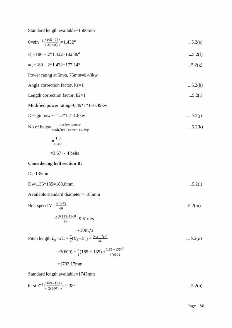
Standard length available=1500mm
θ=sin−1 105−75
2(600) =1.432: …5.2(e)
∝𝑙=180 + 2*1.432=182.86: …5.2(f)
∝𝑠=180 – 2*1.432=177.14: …5.2(g)
Power rating at 5m/s, 75mm=0.49kw
Angle correction factor, k1=1 ...5.2(h)
Length correction factor, k2=1 ...5.2(i)
Modified power rating=0.49*1*1=0.49kw
Design power=1.5*1.2=1.8kw …5.2(j)
No of belts=𝑑𝑒𝑠𝑖𝑔𝑛 𝑝𝑜𝑤𝑒𝑟
𝑚𝑜𝑑𝑖𝑓𝑖𝑒𝑑 𝑝𝑜𝑤𝑒𝑟 𝑟𝑎𝑡𝑖𝑛𝑔 ...5.2(k)
=1.8
0.49
=3.67 ~ 4 belts
Considering belt section B;
D₁=135mm
D₂=1.36*135=183.6mm ...5.2(l)
Available standard diameter = 185mm
Belt speed V= 𝜋𝐷2𝑁1
60 ...5.2(m)
=𝜋 0.135 1360
60=9.61m/s
~10𝑚/𝑠
Pitch length 𝐿𝑝=2C + 𝜋
2(𝐷2+𝐷1) +
(𝐷2−𝐷1)2
4𝐶 …5.2(n)
=2(600) + 𝜋
2(185 + 135) +
(185−135)2
4(600)
=1703.17mm
Standard length available=1745mm
θ=sin−1 185−135
2(600) =2.38: ...5.2(o)
Page | 51
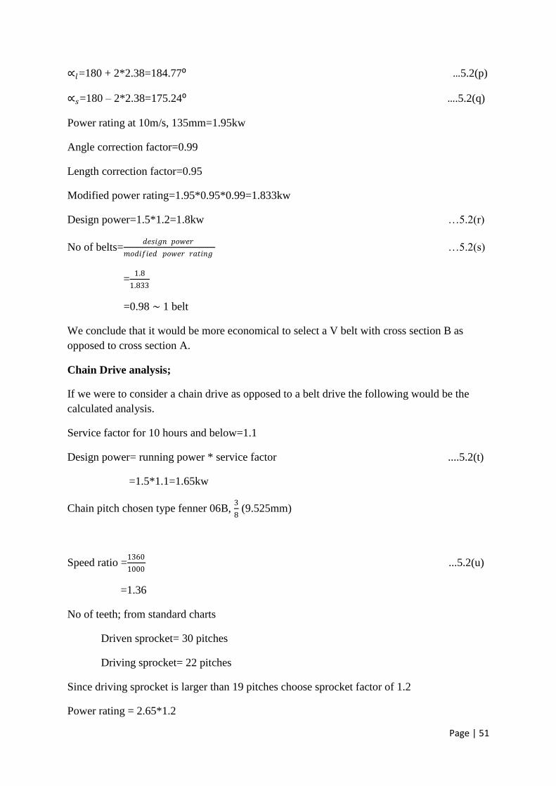
∝𝑙=180 + 2*2.38=184.77: …5.2(p)
∝𝑠=180 – 2*2.38=175.24: ….5.2(q)
Power rating at 10m/s, 135mm=1.95kw
Angle correction factor=0.99
Length correction factor=0.95
Modified power rating=1.95*0.95*0.99=1.833kw
Design power=1.5*1.2=1.8kw …5.2(r)
No of belts=𝑑𝑒𝑠𝑖𝑔𝑛 𝑝𝑜𝑤𝑒𝑟
𝑚𝑜𝑑𝑖𝑓𝑖𝑒𝑑 𝑝𝑜𝑤𝑒𝑟 𝑟𝑎𝑡𝑖𝑛𝑔 …5.2(s)
=1.8
1.833
=0.98 ~ 1 belt
We conclude that it would be more economical to select a V belt with cross section B as
opposed to cross section A.
Chain Drive analysis;
If we were to consider a chain drive as opposed to a belt drive the following would be the
calculated analysis.
Service factor for 10 hours and below=1.1
Design power= running power * service factor ....5.2(t)
=1.5*1.1=1.65kw
Chain pitch chosen type fenner 06B, 3
8 (9.525mm)
Speed ratio =1360
1000 ...5.2(u)
=1.36
No of teeth; from standard charts
Driven sprocket= 30 pitches
Driving sprocket= 22 pitches
Since driving sprocket is larger than 19 pitches choose sprocket factor of 1.2
Power rating = 2.65*1.2

Page | 52
=3.18kw
Chain length, L= 2𝐶
𝑃 +
𝑇+𝑡
2 +
𝐾𝑃
𝐶 …5.2(v)
Where;
L = length of chain in pitches
C = center distance in mm
P = pitch of chain in mm
T = number of teeth on large sprocket
t = number of teeth on small sprocket
K = factor from table
Therefore,
L = 2(600)
9.525 +
30+22
2 +
2(9.525)
600 = 152.01 pitches ....5.2(w)
Rounding off to an even whole number, L=122 pitches
Length of chain in feet = 𝐿𝑃
305 ...5.2(x)
=122∗9.525
305 =4.75 feet
~1.45m
152 pitches or 4.75 feet of Fenner 06B 3
8 in. chain
5.3. APPLICATION / USING THE PROGRAM
The previous section 5.2, shows the theoretical way used for the design and selection of a V-
belt to use when given a certain design problem. However, this may require a high level of
skill in terms of what are the required formulae’s to use and how to apply them to reach a
desired solution.
With the developed V-Belt and Chain Drive C.A.D, its simple and faster to use. Below is a
simple illustration of the above calculations obtained from the C.A.D program.
Step 1; The Data given for the problem:
Motor specification 1.5 kW
Center distance C=600mm
Speed of motor N₁ = 1360RPM

Page | 53
Speed of decorticator machine N₂ =1000RPM
Step 2: load / start the executable program and a MENU page appears.
Select V-belts button, since we intend to perform a V-belt analysis of the design problem.
A new window is then opened for V-belt design commands from the user.
Step 3: Input the design data given above in step 1 and click on the button written CALCULATE.
This then outputs the first set of design options ,e.g. Belt classification available,
belt speed, minimum pitch diameter D1,belt power rating and minimum pitch diameter D2.
A close comparison of the program results to those calculated in section 5.2 are observed to
be similar.
Step 4: Enter an adjacent / closely available standard size for sheave diameter 2.e.g.
185mm and click on the adjust CALCULATE button.
Step 5: Two results are then output as pitch length (mm) and angle of wrap (in radians).
Step 6: Enter an available standard pitch length (from Appendix section A Table 3.2),
Angle of contact correction factor k1 (from Appendix section A Table 3.4) and
Belt length correction factor K2 (from Appendix section A Table 3.5) then click
CALCULATE button.
Step 7: The final result is a modified power rating and number of belts required from which its
advised to base the final selection on the nearest whole number of belts.
Step 8: Use the reset button to clear the form or exit button to close the program.
Page | 54
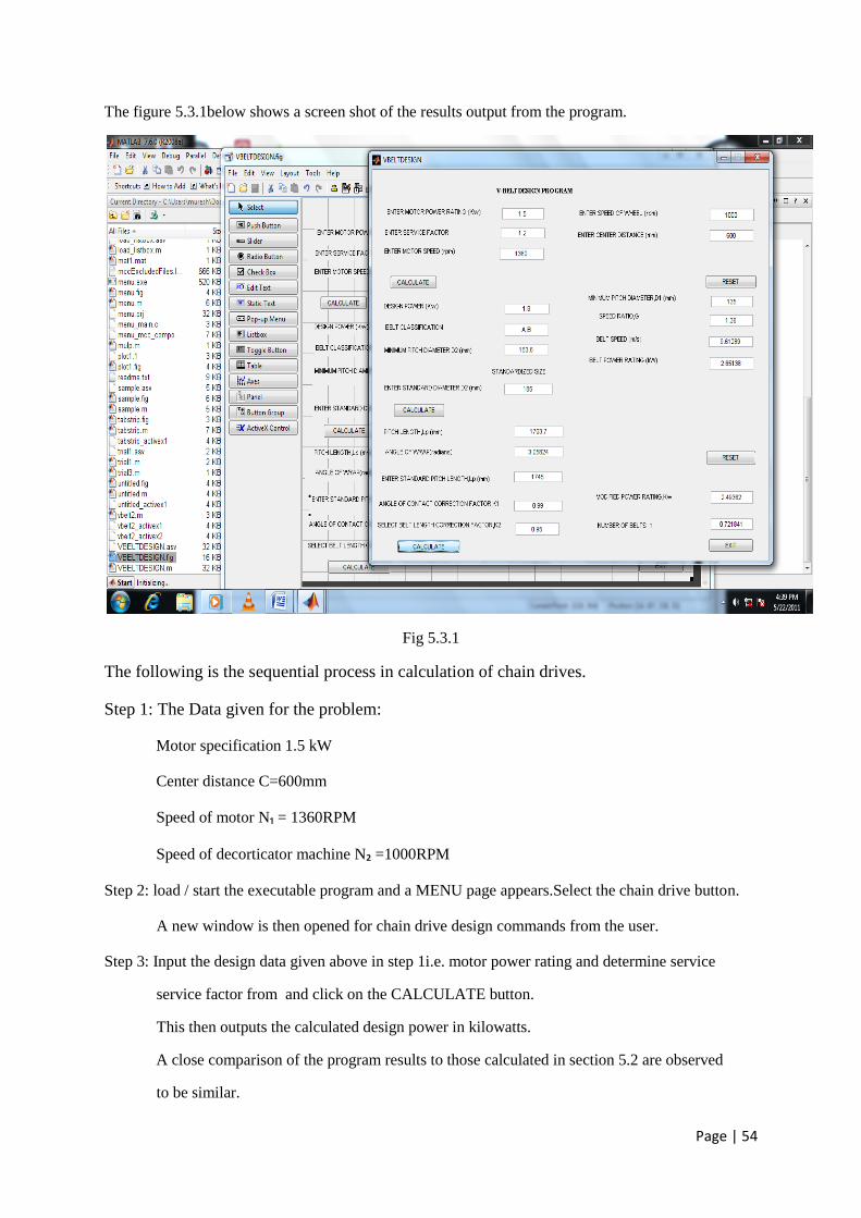
The figure 5.3.1below shows a screen shot of the results output from the program.
Fig 5.3.1
The following is the sequential process in calculation of chain drives.
Step 1: The Data given for the problem:
Motor specification 1.5 kW
Center distance C=600mm
Speed of motor N₁ = 1360RPM
Speed of decorticator machine N₂ =1000RPM
Step 2: load / start the executable program and a MENU page appears.Select the chain drive button.
A new window is then opened for chain drive design commands from the user.
Step 3: Input the design data given above in step 1i.e. motor power rating and determine service
service factor from and click on the CALCULATE button.
This then outputs the calculated design power in kilowatts.
A close comparison of the program results to those calculated in section 5.2 are observed
to be similar.

Page | 55
Step 4: Enter the speed of motor, speed of rotating component or machine, number of teeth of
driving sprocket greater than 17, value of center distance and select the required pitch from
the given drop down list box starting from the smallest value then click on CALCULATE. If
the number of teeth entered is less than 17, there will be a display indicating “inappropriate
teeth”. If the value of pitch selected is wrong there will be a display text indicating
“inappropriate pitch”. If the pitch selected is correct there is a display text indicating
“appropriate pitch”.
Step 5: The program then calculates the speed ratio, number of teeth of larger sprocket, chain pitch
length in pitches, and the pitch diameter of driven and driving sprockets.
Step 6: Use the reset button to clear the form or exit button to close the program.
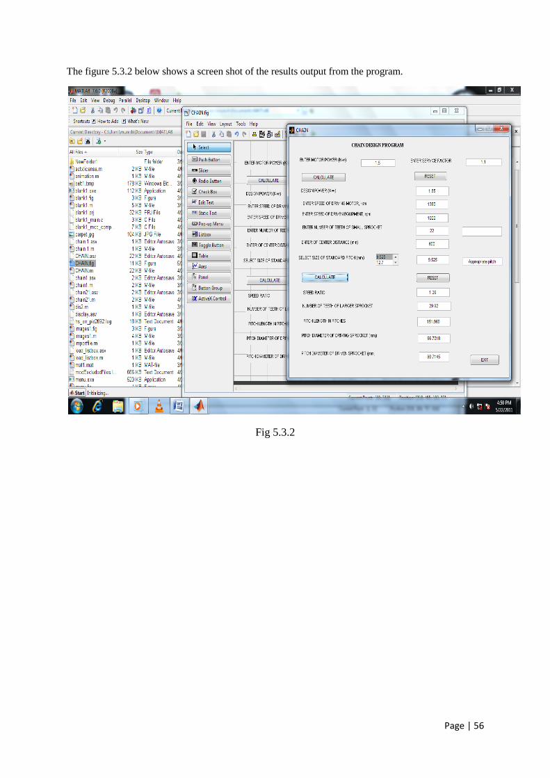
Page | 56
The figure 5.3.2 below shows a screen shot of the results output from the program.
Fig 5.3.2

Page | 57
CHAPTER SIX
6. CLOSURE
6.1. DISCUSSION OF RESULTS
From the above calculations of determining the length of chain in pitches for sisal
decorticator, it was observed that using the manual method of charts and tables, the length of
chain was calculated to be 152.02 pitches, with pitch of 9.525mm. Using our computer aided
program the length was calculated to be 151.969mm, which when rounded off to the nearest
even number comes to 152 pitches with the same pitch of 9.525mm, number of teeth of larger
sprocket determined as 30 and pitch diameters for both driven and driving sprockets as
90.71mm and 66.7mm respectively. Proper selection procedure was observed and the whole
process of selection from manual to use of program was correctly done thus yielding similar
results. We can further conclude that by use of computer aided program, it simplifies the
cumbersome work of using tables and charts and is observed to be a quicker and simpler
method of determining chain length once all the variables needed are known.
In the case of V belt design the important parameters to be determined were belt section,
diameters of both driving and driven pulleys, pitch length, number of belts, angle of wrap and
angle of contact correction factors, and the modified power. The following are the results
obtained from the use of the program;
Belt section B
Driven pitch diameter 183.5mm
Driving pitch diameter 135mm
Speed ratio 1.36
Pitch length 1703.7mm
Angle of contact correction factor 0.99
Belt length correction factor 0.95
Number of belt 0.7218~1
Results obtained by use of theoretical calculations, using design charts and tables are;
Belt section B
Driven pitch diameter 183.6mm
Driving pitch diameter 135mm
Speed ratio 1.36
Pitch length 1703.17mm
Angle of contact correction factor 0.99
Belt length correction factor 0.95
Number of belt 0.98~1
With the same design procedure, it can be shown that the results obtained using the design
program is similar to the results obtained using the charts and tables of design. This indicates
the use of the design program as a substitute to the use of charts and calculations.
Page | 58
6.2. CONCLUSION
The success in integration of theoretical design procedures used for V-belts and chain drive
mechanism into an executable computer program enhanced the realization of the projects
main objectives.
From chapter 5, in the case study, not only was the program developed for design process but
it was also used and tested to check its comparison to theoretical design outcomes. The same
was done for the chain drives and the results obtained considered acceptable.
6.3. RECOMMENDATIONS
Although the development of a computer aided design program for v-Belts and chain drives
was achieved it also can be used as a good baseline for future work. This section presents a
variety of recommendations for future work on improved versions of the program.
1) For the V-belt design section
The program developed is designed to calculate various dimensions input by
the user. However, in some cases the user may / may not be aware of available
standard sizes in the market. Therefore, it would be necessary to find a way of
creating a database preferably a live database so that any new updates of
standard market sizes available can be selected by a user from a list box / drop
down text boxes which are linked to the database.
Visual outputs are a necessity in design as they assist in decision making
based on the outlook revealed by the program. It may be of help that with
more time and resources to invest in a way of using a program that can also
draw the designed object .This will also save time for a designer to draw the
objects manually.
2) For the Chain drive design section
The design of chain drive mechanisms requires visual reading and resultant
input of data from carpet diagrams. In computer programming it is difficult to
find a way of letting the computer pick the accurate co-ordinate from a carpet
diagram since most carpet diagrams are not drawn too even scales.i.e. They
include scale variations. Hence it’s recommended to find a way of using carpet
diagrams to determine the chain pitch to use.
The CAD program developed is based on simplex chains design but further
improvement is necessary in regards to multi-strand chains design. Such as
duplex, triplex chains…etc.

Page | 59
REFERENCES
1. Richard G.Budynas ,J.Keith Nisbett , Shigley`s Mechanical Engineering Design ,8th
edition 2008.
2. Don Sullivan, Belt drive & Bearing systems driving energy responsibility.
3. J.n.Fawcett ,Chain and Belt drives review
4. Prof. M.F Odouri, Friction belt drives and chain drives.
5. Jack A. Collins, Henry R. Busby, George H. Staab ,Mechanical Design of Machine
Elements and Machines
6. Charles E .Wilson ,Computer Integrated Machine Design .
7. Patrick Marchand and O. Thomas Holland, Graphics and GUIs with MATLAB.
8. Math works inc. , Learning MATLAB version 6 ,Getting started guide.
9. Madara ogot, Gul Kremer, Engineering design a practical guide 2004.
10. T.Cicone ,Design of V-Belt transmission (Stas 1163-71 & Iso R 155)
11. IIT khagagpur, Design of V belt drives.
12. Khurmi, R.S. and Gupta J.K., Text book on Machine Design,Eurasia Publishing
House, New Delhi.
13. Wyko Belt Drives.pdf by Wyko industrial services.
14. Carlisle power transmission products inc., Industrial V-belt drives, Design guide.
15. Gates Corporation, Industrial power transmission catalogue.
16. Rexnord Chain Drive Design catalogue.
17. Tsubakimoto chain co. ,The complete guide to chain http://chain-guide.com
18. Renold chain design guide ,“Roller chain catalogue”, http://www.renold.com
19. Cross+morse manufacturers ,catalogue for chain drives, http://www.cross-morse.co.uk
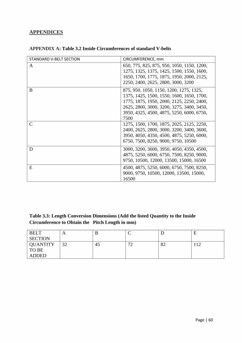
Page | 60
APPENDICES
APPENDIX A: Table 3.2 Inside Circumferences of standard V-belts
STANDARD V-BELT SECTION CIRCUMFERENCE, mm
A 650, 775, 825, 875, 950, 1050, 1150, 1200,
1275, 1325, 1375, 1425, 1500, 1550, 1600,
1650, 1700, 1775, 1875, 1950, 2000, 2125,
2250, 2400, 2625, 2800, 3000, 3200
B 875, 950, 1050, 1150, 1200, 1275, 1325,
1375, 1425, 1500, 1550, 1600, 1650, 1700,
1775, 1875, 1950, 2000, 2125, 2250, 2400,
2625, 2800, 3000, 3200, 3275, 3400, 3450,
3950, 4325, 4500, 4875, 5250, 6000, 6750,
7500
C 1275, 1500, 1700, 1875, 2025, 2125, 2250,
2400, 2625, 2800, 3000, 3200, 3400, 3600,
3950, 4050, 4350, 4500, 4875, 5250, 6000,
6750, 7500, 8250, 9000, 9750, 10500
D 3000, 3200, 3600, 3950, 4050, 4350, 4500,
4875, 5250, 6000, 6750, 7500, 8250, 9000,
9750, 10500, 12000, 13500, 15000, 16500
E 4500, 4875, 5250, 6000, 6750, 7500, 8250,
9000, 9750, 10500, 12000, 13500, 15000,
16500
Table 3.3: Length Conversion Dimensions (Add the listed Quantity to the Inside
Circumference to Obtain the Pitch Length in mm)
BELT
SECTION
A B C D E
QUANTITY
TO BE
ADDED
32 45 72 82 112
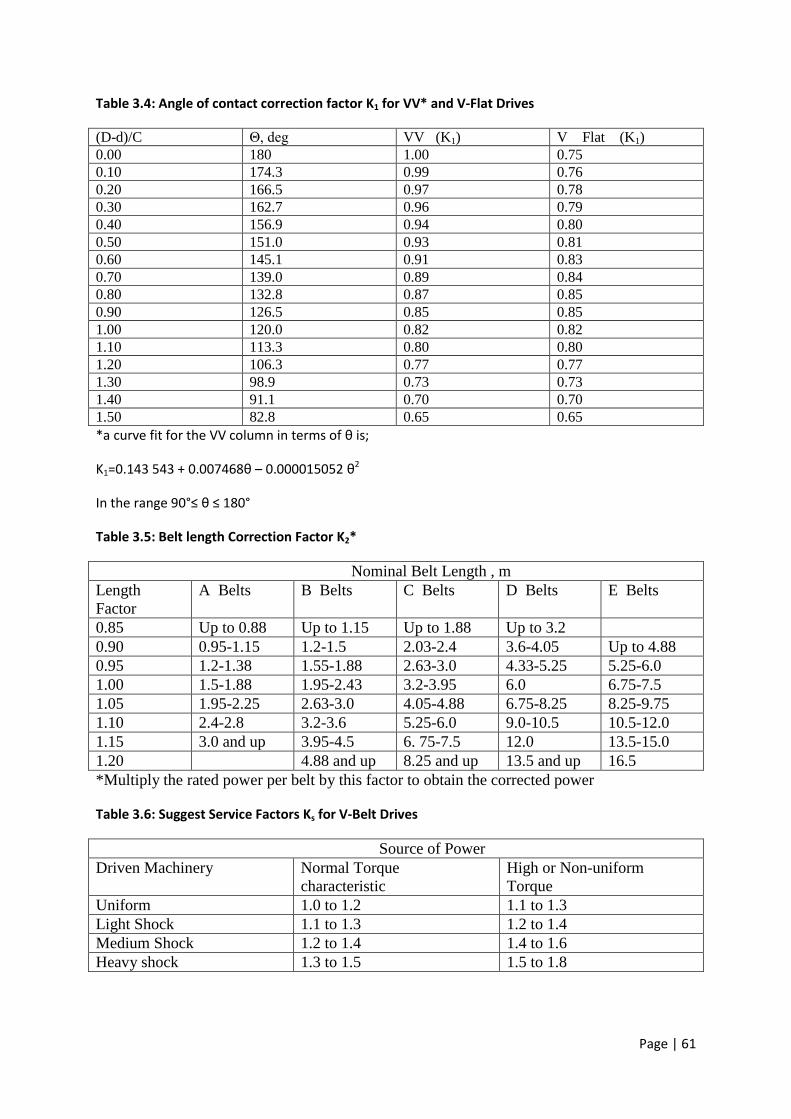
Page | 61
Table 3.4: Angle of contact correction factor K1 for VV* and V-Flat Drives
(D-d)/C Θ, deg VV (K1) V Flat (K1)
0.00 180 1.00 0.75
0.10 174.3 0.99 0.76
0.20 166.5 0.97 0.78
0.30 162.7 0.96 0.79
0.40 156.9 0.94 0.80
0.50 151.0 0.93 0.81
0.60 145.1 0.91 0.83
0.70 139.0 0.89 0.84
0.80 132.8 0.87 0.85
0.90 126.5 0.85 0.85
1.00 120.0 0.82 0.82
1.10 113.3 0.80 0.80
1.20 106.3 0.77 0.77
1.30 98.9 0.73 0.73
1.40 91.1 0.70 0.70
1.50 82.8 0.65 0.65
*a curve fit for the VV column in terms of θ is;
K1=0.143 543 + 0.007468θ – 0.000015052 θ2
In the range 90°≤ θ ≤ 180°
Table 3.5: Belt length Correction Factor K2*
Nominal Belt Length , m
Length
Factor
A Belts B Belts C Belts D Belts E Belts
0.85 Up to 0.88 Up to 1.15 Up to 1.88 Up to 3.2
0.90 0.95-1.15 1.2-1.5 2.03-2.4 3.6-4.05 Up to 4.88
0.95 1.2-1.38 1.55-1.88 2.63-3.0 4.33-5.25 5.25-6.0
1.00 1.5-1.88 1.95-2.43 3.2-3.95 6.0 6.75-7.5
1.05 1.95-2.25 2.63-3.0 4.05-4.88 6.75-8.25 8.25-9.75
1.10 2.4-2.8 3.2-3.6 5.25-6.0 9.0-10.5 10.5-12.0
1.15 3.0 and up 3.95-4.5 6. 75-7.5 12.0 13.5-15.0
1.20 4.88 and up 8.25 and up 13.5 and up 16.5
*Multiply the rated power per belt by this factor to obtain the corrected power
Table 3.6: Suggest Service Factors Ks for V-Belt Drives
Source of Power
Driven Machinery Normal Torque
characteristic
High or Non-uniform
Torque
Uniform 1.0 to 1.2 1.1 to 1.3
Light Shock 1.1 to 1.3 1.2 to 1.4
Medium Shock 1.2 to 1.4 1.4 to 1.6
Heavy shock 1.3 to 1.5 1.5 to 1.8

Page | 62
Table 3.7: Classification of Belt speeds to power rating of standard V-belts.
POWER (Kw) RATING OF STANDARD V-BELTS
BELT
SPEED
(m/s)
V-BELT
SECTION-A
(SHEAVE
PITCH
DIAMETER-
75mm)
V-BELT
SECTION-B
(SHEAVE
PITCH
DIAMETER-
135mm)
V-BELT
SECTION-C
(SHEAVE
PITCH
DIAMETER-
225mm)
V-BELT
SECTION-D
(SHEAVE
PITCH
DIAMETER-
325mm)
V-BELT
SECTION-E
(SHEAVE
PITCH
DIAMETER-
550mm)
5 0.49 1.19 2.49 4.71 8.73
10 0.75 1.95 4.21 7.83 15.14
15 0.84 2.42 5.38 9.7 19.84
20 0.69 2.49 5.86 10.3 22.53
25 0.28 2.1 5.51 9.1 22.75
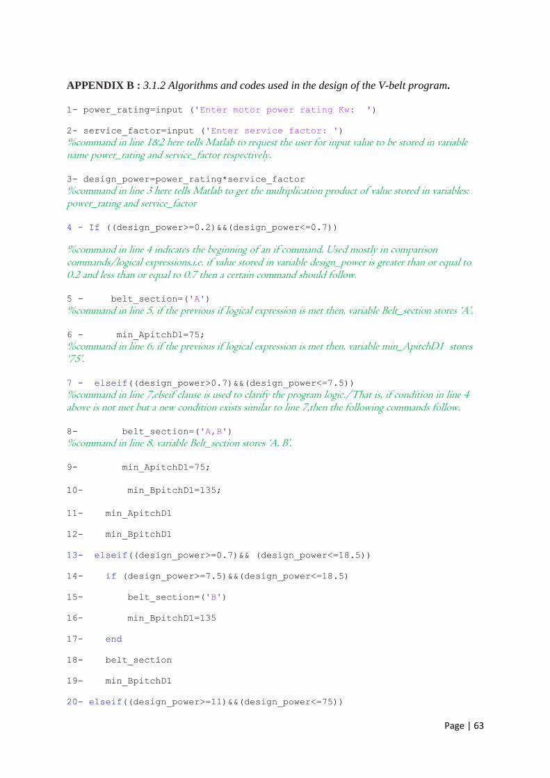
Page | 63
APPENDIX B : 3.1.2 Algorithms and codes used in the design of the V-belt program.
1- power_rating=input ('Enter motor power rating Kw: ')
2- service_factor=input ('Enter service factor: ')
%command in line 1&2 here tells Matlab to request the user for input value to be stored in variable name power_rating and service_factor respectively. 3- design_power=power_rating*service_factor
%command in line 3 here tells Matlab to get the multiplication product of value stored in variables: power_rating and service_factor 4 - If ((design_power>=0.2)&&(design_power<=0.7))
%command in line 4 indicates the beginning of an if command. Used mostly in comparison commands/logical expressions.i.e. if value stored in variable design_power is greater than or equal to 0.2 and less than or equal to 0.7 then a certain command should follow. 5 - belt_section=('A')
%command in line 5, if the previous if logical expression is met then, variable Belt_section stores ‘A’. 6 - min_ApitchD1=75;
%command in line 6, if the previous if logical expression is met then, variable min_ApitchD1 stores ‘75’. 7 - elseif((design_power>0.7)&&(design_power<=7.5))
%command in line 7,elseif clause is used to clarify the program logic./That is, if condition in line 4 above is not met but a new condition exists similar to line 7,then the following commands follow. 8- belt_section=('A,B')
%command in line 8, variable Belt_section stores ‘A, B’. 9- min_ApitchD1=75;
10- min_BpitchD1=135;
11- min_ApitchD1
12- min_BpitchD1
13- elseif((design_power>=0.7)&& (design_power<=18.5))
14- if (design_power>=7.5)&&(design_power<=18.5)
15- belt_section=('B')
16- min_BpitchD1=135
17- end
18- belt_section
19- min_BpitchD1
20- elseif((design_power>=11)&&(design_power<=75))
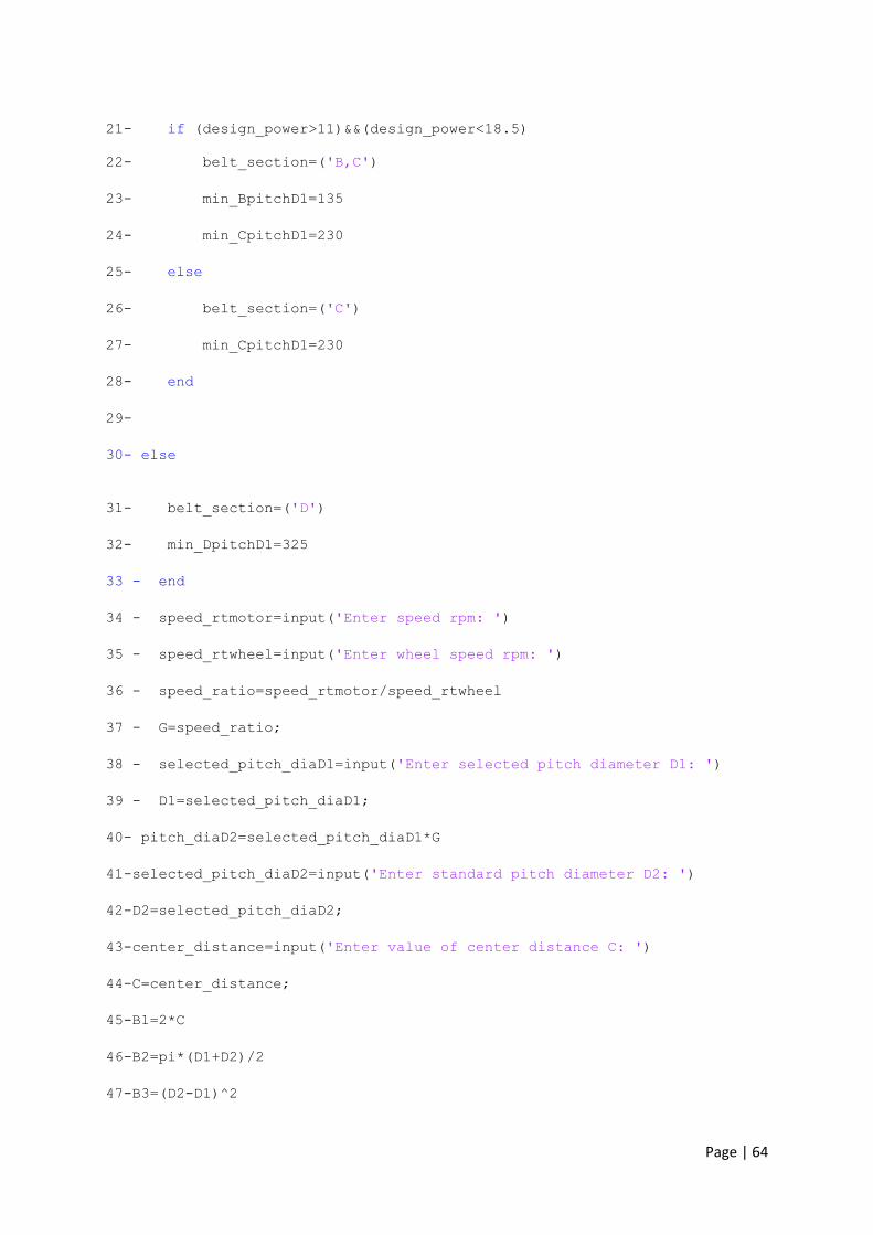
Page | 64
21- if (design_power>11)&&(design_power<18.5)
22- belt_section=('B,C')
23- min_BpitchD1=135
24- min_CpitchD1=230
25- else
26- belt_section=('C')
27- min_CpitchD1=230
28- end
29-
30- else
31- belt_section=('D')
32- min_DpitchD1=325
33 - end
34 - speed_rtmotor=input('Enter speed rpm: ')
35 - speed_rtwheel=input('Enter wheel speed rpm: ')
36 - speed_ratio=speed_rtmotor/speed_rtwheel
37 - G=speed_ratio;
38 - selected_pitch_diaD1=input('Enter selected pitch diameter D1: ')
39 - D1=selected_pitch_diaD1;
40- pitch_diaD2=selected_pitch_diaD1*G
41-selected_pitch_diaD2=input('Enter standard pitch diameter D2: ')
42-D2=selected_pitch_diaD2;
43-center_distance=input('Enter value of center distance C: ')
44-C=center_distance;
45-B1=2*C
46-B2=pi*(D1+D2)/2
47-B3=(D2-D1)^2
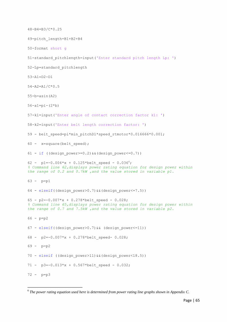
Page | 65
48-B4=B3/C*0.25
49-pitch_length=B1+B2+B4
50-format short g
51-standard_pitchlength=input('Enter standard pitch length Lp: ')
52-Lp=standard_pitchlength
53-A1=D2-D1
54-A2=A1/C*0.5
55-b=asin(A2)
56-a1=pi-(2*b)
57-k1=input('Enter angle of contact correction factor k1: ')
58-k2=input('Enter belt length correction factor: ')
59 - belt_speed=pi*min_pitchD1*speed_rtmotor*0.016666*0.001;
60 - x=square(belt_speed);
61 - if ((design_power>=0.2)&&(design_power<=0.7))
62 - p1=-0.004*x + 0.125*belt_speed - 0.0366;
% Command line 62,displays power rating equation for design power within
the range of 0.2 and 0.7kW ,and the value stored in variable p1.
63 - p=p1
64 - elseif((design_power>0.7)&&(design_power<=7.5))
65 - p2=-0.007*x + 0.278*belt_speed - 0.028;
% Command line 65,displays power rating equation for design power within
the range of 0.7 and 7.5kW ,and the value stored in variable p2.
66 - p=p2
67 - elseif((design_power>0.7)&& (design_power<=11))
68 - p2=-0.007*x + 0.278*belt_speed- 0.028;
69 - p=p2
70 - elseif ((design_power>11)&&(design_power<18.5))
71 - p3=-0.013*x + 0.567*belt_speed - 0.032;
72 - p=p3
6 The power rating equation used here is determined from power rating line graphs shown in Appendix C.
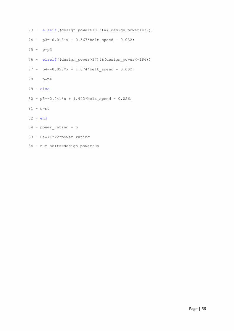
Page | 66
73 - elseif((design_power>18.5)&&(design_power<=37))
74 - p3=-0.013*x + 0.567*belt_speed - 0.032;
75 - p=p3
76 - elseif((design_power>37)&&(design_power<=186))
77 - p4=-0.028*x + 1.074*belt_speed - 0.002;
78 - p=p4
79 – else
80 - p5=-0.041*x + 1.942*belt_speed - 0.026;
81 - p=p5
82 – end
84 – power_rating = p
83 - Ha=k1*k2*power_rating
84 - num_belts=design_power/Ha
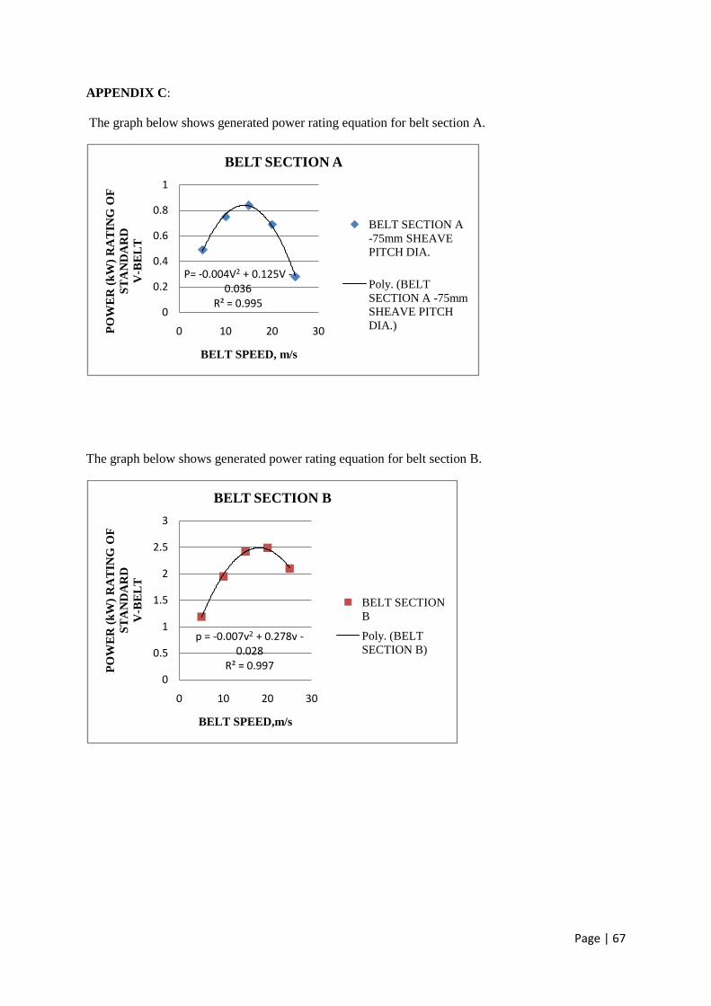
Page | 67
APPENDIX C:
The graph below shows generated power rating equation for belt section A.
The graph below shows generated power rating equation for belt section B.
P= -0.004V2 + 0.125V -0.036
R² = 0.9950
0.2
0.4
0.6
0.8
1
0 10 20 30PO
WE
R (
kW
) R
AT
ING
OF
ST
AN
DA
RD
V-B
EL
T
BELT SPEED, m/s
BELT SECTION A
BELT SECTION A
-75mm SHEAVE
PITCH DIA.
Poly. (BELT
SECTION A -75mm
SHEAVE PITCH
DIA.)
p = -0.007v2 + 0.278v -0.028
R² = 0.9970
0.5
1
1.5
2
2.5
3
0 10 20 30
PO
WE
R (
kW
) R
AT
ING
OF
ST
AN
DA
RD
V-B
EL
T
BELT SPEED,m/s
BELT SECTION B
BELT SECTION
B
Poly. (BELT
SECTION B)
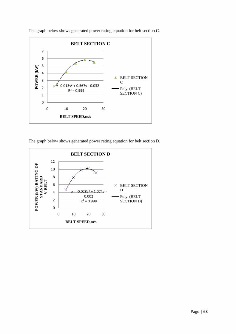
Page | 68
The graph below shows generated power rating equation for belt section C.
The graph below shows generated power rating equation for belt section D.
p = -0.013v2 + 0.567v - 0.032R² = 0.999
0
1
2
3
4
5
6
7
0 10 20 30
PO
WE
R (
kW
)
BELT SPEED,m/s
BELT SECTION C
BELT SECTION
C
Poly. (BELT
SECTION C)
p = -0.028v2 + 1.074v -0.002
R² = 0.998
0
2
4
6
8
10
12
0 10 20 30
PO
WE
R (
kW
) R
AT
ING
OF
ST
AN
DA
RD
V-B
EL
T
BELT SPEED,m/s
BELT SECTION D
BELT SECTION
D
Poly. (BELT
SECTION D)
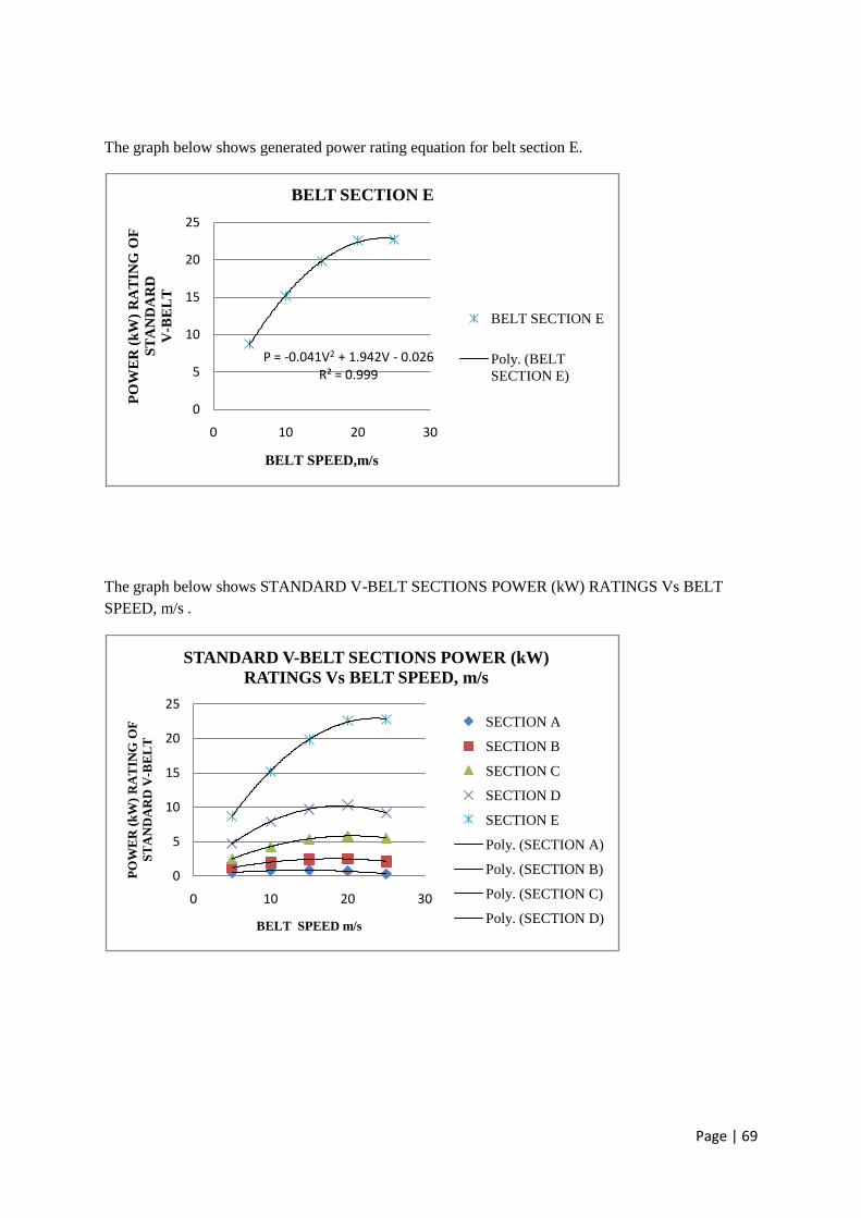
Page | 69
The graph below shows generated power rating equation for belt section E.
The graph below shows STANDARD V-BELT SECTIONS POWER (kW) RATINGS Vs BELT
SPEED, m/s .
P = -0.041V2 + 1.942V - 0.026R² = 0.999
0
5
10
15
20
25
0 10 20 30
PO
WE
R (
kW
) R
AT
ING
OF
ST
AN
DA
RD
V-B
EL
T
BELT SPEED,m/s
BELT SECTION E
BELT SECTION E
Poly. (BELT
SECTION E)
0
5
10
15
20
25
0 10 20 30
PO
WE
R (
kW
) R
AT
ING
OF
ST
AN
DA
RD
V-B
EL
T
BELT SPEED m/s
STANDARD V-BELT SECTIONS POWER (kW)
RATINGS Vs BELT SPEED, m/s
SECTION A
SECTION B
SECTION C
SECTION D
SECTION E
Poly. (SECTION A)
Poly. (SECTION B)
Poly. (SECTION C)
Poly. (SECTION D)

Page | 70
Table 4.1 service factors for chain drive.
Characteristics of
driven machine
Characteristics of driver
Smooth running Slight shock Moderate shock
Smooth running 1.0 1.1 1.3
Moderate shock 1.4 1.5 1.7
Heavy shock 1.8 1.9 2.1
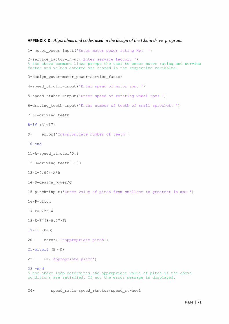
Page | 71
APPENDIX D : Algorithms and codes used in the design of the Chain drive program.
1- motor_power=input('Enter motor power rating Kw: ')
2-service_factor=input('Enter service factor: ')
% the above command lines prompt the user to enter motor rating and service
factor and values entered are stored in the respective variables.
3-design_power=motor_power*service_factor
4-speed_rtmotor=input('Enter speed of motor rpm: ')
5-speed_rtwheel=input('Enter speed of rotating wheel rpm: ')
6-driving_teeth=input('Enter number of teeth of small sprocket: ')
7-Z1=driving_teeth
8-if (Z1<17)
9- error('Inappropriate number of teeth')
10-end
11-A=speed_rtmotor^0.9
12-B=driving_teeth^1.08
13-C=0.004*A*B
14-D=design_power/C
15-pitch=input('Enter value of pitch from smallest to greatest in mm: ')
16-P=pitch
17-F=P/25.4
18-E=F^(3-0.07*F)
19-if (E<D)
20- error('Inappropriate pitch')
21-elseif (E>=D)
22- P=('Appropriate pitch')
23 –end
% the above loop determines the appropriate value of pitch if the above
conditions are satisfied. If not the error message is displayed.
24- speed_ratio=speed_rtmotor/speed_rtwheel
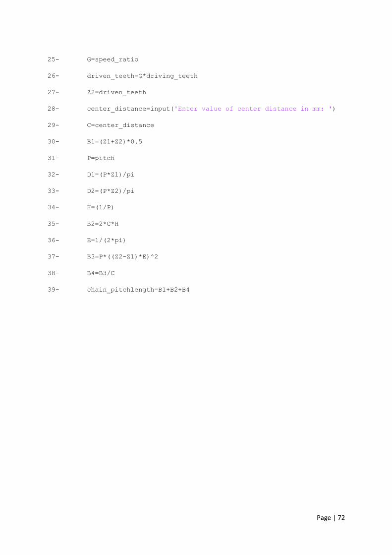
Page | 72
25- G=speed_ratio
26- driven_teeth=G*driving_teeth
27- Z2=driven_teeth
28- center_distance=input('Enter value of center distance in mm: ')
29- C=center_distance
30- B1=(Z1+Z2)*0.5
31- P=pitch
32- D1=(P*Z1)/pi
33- D2=(P*Z2)/pi
34- H=(1/P)
35- B2=2*C*H
36- E=1/(2*pi)
37- B3=P*((Z2-Z1)*E)^2
38- B4=B3/C
39- chain_pitchlength=B1+B2+B4
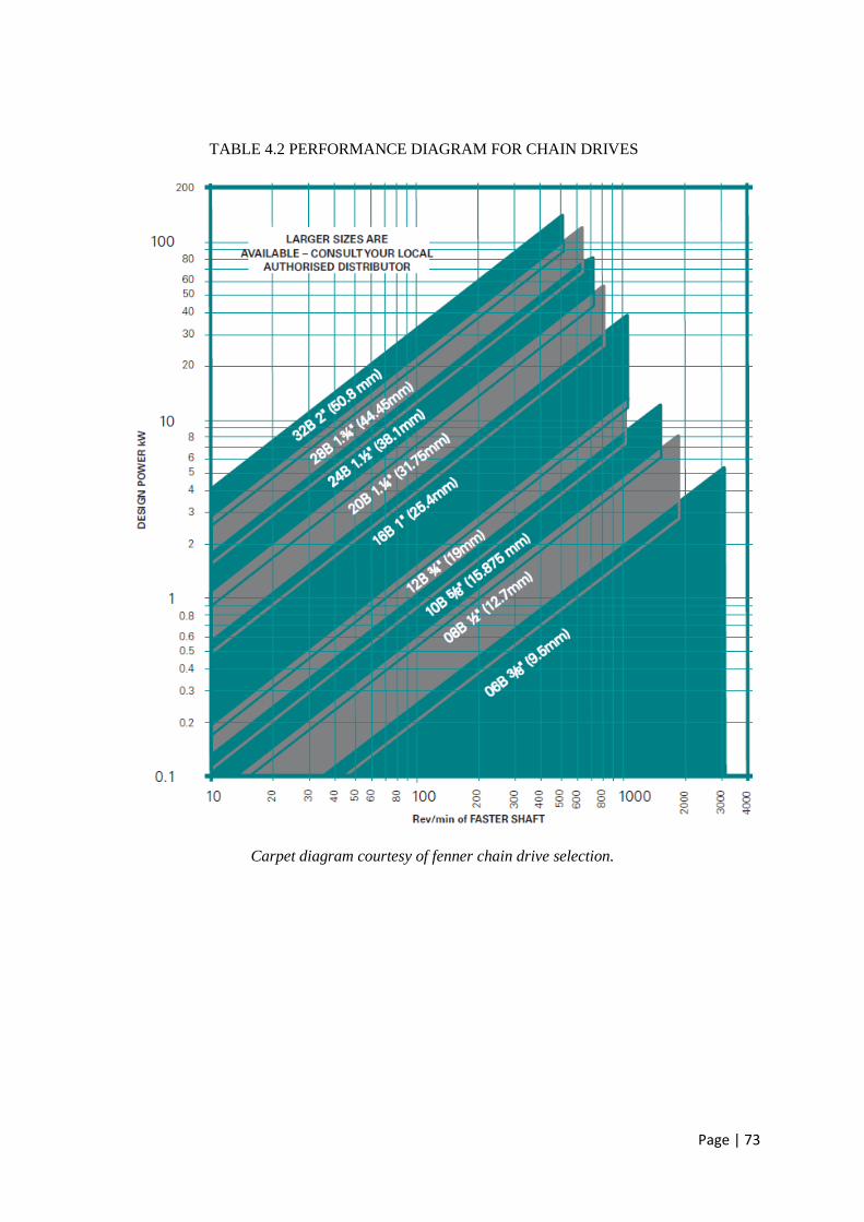
Page | 73
TABLE 4.2 PERFORMANCE DIAGRAM FOR CHAIN DRIVES
Carpet diagram courtesy of fenner chain drive selection.

Page | 74
TABLE 4.3 RATIO OF NUMBER OF TEETH OF SPROCKETS
Table courtesy of fenner chain drive selection.