Scanning Force Microscopy And Related Techniques

Danny Porath 2003

With the help of…….

1. Yosi Shacham – TAU2. Yossi Rosenwacks – TAU3. Julio Gomez-Herrero – UAM4. Adriana Gil - UAM5. Serge Lemay - Delft6. Hezy Cohen - HUJI7. …

Outline AFM:1. Examples, links and homework

2. AFM principle and structure

3. Tip-surface interactions

4. Feedback techniques

5. Force-distance curves and modes of operation

6. The scanner

7. Tip convolution and resolution

8. Cantilevers and tips

Books and Internet Sites“Scanning Probe Microscopy and Spectroscopy”, R. Wiesendanger

“Scanning Force Microscopy”, D. Sarid

http://www.embl-heidelberg.de/~altmann/http://www.uam.es/departamentos/ciencias/fismateriac/especifica/Nuevas%20Microscopies%20webpage/pdfs/Thesis_A_Gil.pdf

http://www.eng.tau.ac.il/~yosish/courses.htmlhttp://www.eng.tau.ac.il/~yossir/course/

http://www.chembio.uoguelph.ca/educmat/chm729/STMpage/stmtutor.htmhttp://www.weizmann.ac.il/surflab/peter/afmworks/index.html

http://www.cmmp.ucl.ac.uk/~asf/physics/Ncafm.htmlhttp://www.bam.de/english/expertise/areas_of_expertise/department_6/division_62/laboratory_621.htm

http://spm.phy.bris.ac.uk/welcome.htmlhttp://wwwex.physik.uni-ulm.de/en_wissensch.htm

http://chemistry.jcu.edu/mwaner/research/afm/http://spm.aif.ncsu.edu/tutorial.htm....

Homework 61. Read the paper:

“The millipede – more than one thousand tips for future AFM data storage”By: Vettiger et. al., IBM Journal of Research and Development 44, 323 (2000)- Emphasize the “lithography” part.

2. Find on the web, in a paper or in a book the 3 most impressive SPM (not STM) images:

a. 1 - Technicallyb. 1 - Scientificallyc. 1 - Aesthetically

Explain your choice. If needed compare with additional images.3. For “Maskianim” – Read the “practical Guide for SPM” (in my notes or in:

http://www.topometrix.com/spmguide/contents.htm)

Schematic of Generalized AFM

Contact to Surface…

Monitored by Laser…

Obtaining Surface Profiles

The tip is attached to a piezoelectric and scans the surface

ss

x

xy

SFM Block Diagram Personal

Computer

SPM Signals

HV Amplifiers and signal conditioning

SPM tip

Signal detector

Piezoelectric scanner

SFM 3 dimensional image of a tumor cell HeLa (37x37µm2)

Digital

SignalProcessor

SFM Head Vibration isolation + Stiffness

1cm

Laser diode

Window for optical microscope

Beam adjustment Photodiode

Coarse approach

Piezoelectric scanner

Photodiode adjustment

system

Vibration Isolation

kd

km

ω∝k2ωd as small as possible (2Hz)

ωm as high as possible (2kHz){

ωd ωmω

ADumping StiffnessMechanical

loop

Stiffness scales with size. SPM as small as possible

The First AFM Binnig, Quate, and Gerber invented the AFM in 1986 mainly due to the limitations of the STM

The first AFM image was Al2O3 imaged with a diamond tip mounted on a gold cantilever, and tunneling was used for force detection.

AFM Images

Magnetic bits of a zip disk G4-DNA

100nm10µm

DNA-NanotubeNanotube between

electrodes

F= -kz, k= E/4·W·(T/L)3

k depends on the geometry and material

0.1 mm

T=

5 µm

L=0.1 mm

W=

20 µ

m

z

E- Young modulus, W- width, T – thickness, L - length

The Microcantilever and Hook’s Law

More about springs

222220 4)(

)(ωβωω

ω⋅⋅+−

=AD

F0 cos(ωt)

ω

Q

74000 76000 78000 80000 82000 84000 860000

20

40

60

80

100

Q=100 (in air)Q=50Q=10 (in liquids)

D( ω

)/D(0

)

(rad/s)

The resonance frequency of the cantilever also depends on the geometry and material, for a rectangular cantilever:

ω0=0.162·(E/ρ)1/2·T/L2

Tip-Surface Interaction

Tip- sample distance

F<0 Attractive

U(z

)

F>0 Repulsive

Potential

Interatomic forces vs. distance curve

|Fvdw|=|Fion|+|Fel|

Force

Forces During Approach

AFM Principle and Tip-Surface Interaction Interatomic forces vs. distance curve

|Fvdw|=|Fion|+|Fel|

612 //)( rArBrw −= 713 /6/12)( rArBdrdWrF −=−≡⇒

Tip-Surface Interaction

Repulsion forces: incomplete screening of nuclear charge, Pauli exclusion principleDue to the sharpness and size of the tip, long range forces (like electrostatic) and hence many-body-interactions play the dominant role.Electrostatic forces (attractive) play the dominant role at distances greater then 10 nm (simple parallel-plate capacitor model)

The Two Springs Model

The distances represent:z-tip-sample distance, d-cantilever deflection, ∆-cantilever-sample distance (=piezo movement)∆z=d+z

Vtot(z,∆)=Vsurf(z)+1/2Clev(∆-z)2

The total energy:

The position of the tip for an equilibrium situation is determined by the force balance:

z)(∆Cz

Vz

V∆)F(z, levsurftot

−+∂

∂=

∂∂

≡

The stability condition can be obtained from:

022

≥+∂

∂+=

∂∂

≡ lev2surf

2tot

eff Cz

VzV∆)(z,C

Clev – Cantilever spring constant

Equilibrium Situation

Two terms must be added:External excitation forceDamping term (proportional to the tip velocity)

The external force:

tz

Qmω-(t)Fz)(∆C

zV

tzm 00

extlevsurf

2

2

∂∂

+−+∂

∂=

∂∂

The equation of motion:

Dynamic SFM The cantilever is oscillated at its resonance frequency:

Q – quality factor, ω00- resonance frequency

t)(ωF (t)F 000ext cos=

A quadratic interaction potential changes the effective spring constant :

The resonance frequency shifts:

lev

pot00

eff

eff0 C

C1ω

m(z)Cω +==

The resonance frequency for a small free oscillation:Dynamic SFM

eff

lev00 m

Cω = meff~0.24 mlever

V(z)=Cpotz2 Ceff=Clev+V"

Amplitude and Phase Curves for a Damped Harmonic Oscillator

However …. In reality the potential is not quadratic and the oscillation is not small ….So …. more complicated non-linear models have to be applied…☺

Relevant Interactions in SFM

The vibration frequency of atoms, ω, at room temperature ~ 1015 HzThe mass, m, of an atom ~ 10-30 kgThe effective spring constant, k, between atoms is:

k= ω2m ≈ 1N/m

Relevant Interactions in SFMRepulsive interaction and contact force:

At very small tip-sample distances (a few angstroms) a very strong repulsive force appears between the tip and sample atoms. Its origin is the so-called exchange interactions due to the overlap of the electronic orbitals at interatomic distances.

When this repulsive force is predominant, the tip and sample are considered to be in “contact”.

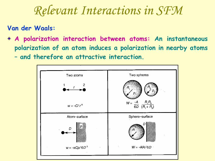
Relevant Interactions in SFMVan der Waals:

A polarization interaction between atoms: An instantaneous polarization of an atom induces a polarization in nearby atoms – and therefore an attractive interaction.

Relevant Interactions in SFMMagnetic interaction:

Caused by magnetic dipoles both on the tip and the sample. This interaction is used for Magnetic Force Microscopy to study magnetic domains on the sample surface.

Electrostatic interaction:Caused by both the localized charges and the polarization of the substrate due to the potential difference between the tip and the sample. It has been used to study the electrostatic properties of samples such as microelectronic structures, charges on insulator surfaces, or ferroelectric domains.

Relevant Interactions in SFMFriction and adhesion:

The SFM cantilever bends laterally due to a friction forcebetween the tip and the sample surfaces.Adhesion can be defined as “the free energy change to separate unit areas of two media from contact to infinity in vacuum or in a third medium”. In general, care has to be taken with the term adhesionsince it is also used to define a force - the adhesion force, as for example in SFM. In SFM at ambient conditions in addition to the intrinsic adhesion between tip and sample there is another one from the capillary neck condensing between them. Then, the pull-off force is considered as the adhesion force, which is in the range of a few nanonewton to tens of nanonewton.

Wetting Situations

Adhesion (due to water meniscus)

The snap-in distance increases depending on the relative humidity, up to 10-15 nm.

Fadh=4πR(γlgcosθ+γsl)=4pR γlg

θ – contact angel, λsl, λlg, λlg, – surface energies at solid/liquid, liquid/gas and solid/gas interfaces.

Detecting Cantilever Deflection

a) STM tipb) Capacitancec) Beam defection

Cantilever Deflection Measurement: Tunneling

Disadvantages:Difficult alignmentSensitivity of ~0.01 Å, but extremely sensitive to surface conditionsThermal drifts, local changes in barrier height affect force measurements

The Beam Deflection Method

a) Normal force

UP

Down

A+B= UP

C+D=DOWN

b)Lateral Force

Right

left A+C= LEFT

B+D=Right

Photodiode

Laser

The Feedback in SFM

The normal force is kept constant using the feedback

Piezoelectric material:changes its shape when an electric potential is applied

+- sum

+ - Set Point

PID

Amplification

DSP and Data

Acquisiton Board

ADCD

AC

sum

Advantages:

• Negligible force on cantilever

• Not very sensitive to cantilever surface

• Disadvantage: Sample illumination

Forces During Approach

This technique is used to measure the normal force vs. distance

It can be used to measure similarly any other quantity: Lateral force, electrostatic force etc.

Can be used to study contaminations, viscosity …..

Forces vs. DistanceThis technique is used to measure the normal force vs.distance.

A force vs.distance curve is a plot of the deflection of the cantilever versus the extension of the piezoelectric scanner,measured using a position-sensitive photodetector.

It can be used to measure similarly any other quantity: Lateral force, amplitude, phase, current etc.

Can be used to study contaminations, viscosity, lubrication thickness,and local variations in the elastic properties of the surface.

Contact AFM can be operated anywhere along the linear portion of the force vs. distance curves.

Forces-Distance at Various Environments

AirWater

Air+contamination

Contact Mode and Dynamic Mode

In contact mode the deflection of the cantilever is kept constant

In dynamic mode the tip is oscillated at the resonance frequency and the amplitude of the oscillation is kept constant

Surface interaction

AFM: Non-contact and Tapping

Non-Contact and Tapping: frequency of operation

Feedback Mechanism

Tapping: provides high resolution with less sample damage

“Free” amplitude

“Reduced” amplitude

Fluid layer“tapping”

AFM: Dynamic Mode

Force vs. Distance: Dynamic Mode

Contact, Non-Contact, Tapping

Contact mode imaging (left) is heavily influenced by frictional and adhesive forces which can damage samples and distort image data. Non-contactimaging (center) generally provides low resolution and can also be hampered by the contaminant layer which can interfere with oscillation. Tapping Mode imaging (right) eliminates frictional forces by intermittently contacting the surface and oscillating with sufficient amplitude to prevent the tip from being trapped by adhesive meniscus forces from the contaminant layer. The graphs under the images represent likely image data resulting from the three techniques.

Contact vs. Tapping – Si (100)

Tapping Mode images show no surface alteration and better resolution.

Contact imaging shows clear surface damage. Material has been removed by the scanning tip, while in other cases, additional oxide growth or more subtle changes may occur.

This type of surface alteration often goes undetected since not all researchers check for damage by rescanning the affected area at lower magnification.

1µm 2 µm 2 µm1µmContact Tapping

1st scan 2nd scan 1st scan 2nd scan

Non-Contact vs. Contact Through Water

Non-Contact Contact

Constant Height and Constant ForceConstant Height:In constant-height mode, the spatial variation of the cantilever deflection can be used directly to generate the topographic data set because the height of the scanner is fixed as it scans.

Constant-height mode is often used for taking atomic-scale images of atomically flat surfaces, where the cantilever deflections and thus variations in applied force are small. Constant-height mode is also essential for recording real-time images of changing surfaces,where high scan speed is essential.

Constant Force: In constant-force mode,the deflection of the cantilever can be used as input to a feedback circuit that moves the scanner up and down in z ,responding to the topography by keeping the cantilever deflection constant. In this case,the image is generated from the scanner’s motion. With the cantilever deflection held constant,the total force applied to the sample is constant.

In constant-force mode,the speed of scanning is limited by the response time of the feedback circuit, but the total force exerted on the sample by the tip is well controlled. Constant-force mode is generally preferred for most applications.

Magnetic Force Microscopy (MFM)

Magnetic force microscopy (MFM) images the spatial variation of magnetic forces on a sample surface.

MFM operates in non-contact mode, detecting changes in the resonant frequency of the cantilever induced by the magnetic field’s dependence on tip-to-sample separation.

MFM image of a hard disk (30 µm)

Lateral Force Microscopy (LFM)

LFM measures lateral deflections (twisting) of the cantilever that arise from forces on the cantilever parallel to the plane of the sample surface.

LFM images variations in surface friction, arising from inhomogeneity in surface material, obtaines edge-enhanced (slope variations) images of any surface.

To separate the effects AFM and LFM should be used simultaneously.

Lateral deflection by friction variations

Lateral deflection by slope variations

Force Modulation Microscopy (FMM)

In FMM mode, the tip is scanned in contact with the sample, and the z feedback loop maintains a constant cantilever deflection (as for constant-force mode AFM).A periodic signal is applied to either the tip or the sample. The amplitude of cantilever modulation that results from this applied signal varies according to the elastic properties of the sample.The system generates a force modulation image, which is a map of the sample's elastic properties, from the changes in the amplitude of cantilever modulation.The frequency of the applied signal is on the order of hundreds of kHz, which is faster than the z feedback loop is set up to track. Thus, topographic information can be separated from local variations in the sample's elastic properties, and the two types of images can be collected simultaneously.

FMM of Carbon fiber/polymer Composite Collected Simultaneously (5µm)

Contact AFM FMM

Phase Imaging

Phase detection monitors the phase lag between the signal that drives the cantilever to oscillate and the cantilever oscillation output signal.phase imaging is used to map variations in surface properties such as elasticity, adhesion and friction.Phase detection images can be produced while an instrument is operating in any vibrating cantilever mode.The phase lag is monitored while the topographic image is being taken so that images of topography and material properties can be collected simultaneously.

Phase Imaging of an Adhesive Label (3 µm)

Non-contact AFM Phase image

Electrostatic Force Microscopy (EFM)

In EFM voltage is applied between the tip and the sample while the cantilever hovers above the surface, not touching it. The cantilever deflects when it scans over static charges. The magnitude of the deflection, proportional to the charge density, can be measured with the standard beam-bounce system.EFM plots the locally charged domains of the sample surface.EFM is used to study the spatial variation of surface charge carrier density. For instance, EFM can map the electrostatic fields of a electronic circuit as the device is turned on and off.

Electrostatic Interaction Upon Voltage Application

Total electrostatic force

Additional Force Microscopy Techniques

Scanning capacitance microscopy (SCM)

Scanning thermal microscopy (SThM)

Near field scanning optical microscopy (NSOM)

Kelvin probe microscopy

Scanning spreading resistance microscopy

Contact Potential Difference (CPD)

Pulsed force mode (PFM)

3D mode

Jumping mode

AFM Scanning

S – Strain [Å/m], d – Strain coefficient [Å/V], E – Electric field [V/m]

S=dE

Ideally, a piezoelectric scanner varies linearly with applied voltage.

Piezo tube Raster scan

Intrinsic Nonlinearity

Ideally, The intrinsic nonlinearity is the ratio ∆y/y of the maximum deviation ∆y from the linear behavior to the ideal linear extension y at that voltage.It is in the range 2-25%.

∆y

y

Scanner Hystersis

The hysteresis of a piezoelectric scanner is the ratio of the maximum divergence between the two curves to the maximum extension that a voltage can create in the scanner: ∆Y/Ymax. Hysteresis can be as high as 20% in piezoelectric materials.

Scanner Creep

When an abrupt change in voltage is applied, the piezoelectric reacts in two steps: the first step takes place in less than a millisecond, the second on a much longer time scale. The second step, ∆xc, is known as creep.Creep is the ratio of the second dimensional change to the first: ∆x c /∆x. It ranges from 1%to 20%, over times of 10 to 100 sec.

Scanner Aging

The aging rate is the change in strain coefficient per decade of time.The piezoelectric coefficient, d, changes exponentially with time: increase with regular use, decrease with no use.

Scanner Cross Coupling

Geometric effect: The x-y motion of a scanner tube is produced when one side shrinks and the other expands.Can be corrected with image-processing software, checked using a sample with a known curvature (lens).

Software Correction

Hardware Correction

A sensor “reads” the scanner actual position, and a feedback system applies voltage to drive the scanner to the desired position, the total nonlinearity can be reduced to 1%.

Tip Convolution

Tip Convolution - example

AFM image Cross sectionNominal width 180 nm Measured width 350 nm

Resolution

Tip convolution is not linear: results do not add up!!!The resolution depends on tip AND sample.

Convolution Test by Rotation

Tip imaging: the image does not change upon rotationTrue imaging: the image rotates upon scan direction rotation.

Additional Artifacts

Convolution with other “physics” (sample charging, stiffness, contamination etc.)

Feedback artifacts

External noise and fields

….

Tests for ArtifactsRepeat the scan to ensure that it looks the same.

Change the scan direction and take a new image.

Change the scan size and take an image to ensure that the features scale properly.

Rotate the sample and take an image to identify tip imaging

Change the scan speed and take another image (especially if you see suspicious periodic or quasi-periodic features).

The Force Sensor – The Tip

The Force Sensor – The Tip

o

A 300 -radii Tip

NSi and SiO -scantiliver Comercialthickness -t lenght, -l width,w

ModuleYoung -E

,l4

Ewtk

432

3

3

−

=

The Force Sensor – The Tip

The Force Sensor – The Tip

Diamond-coated tip FIB-sharpened tip

Gold-coated Si3N4 tip

Tip Fabrication

Pit etching in Si Si underetchingSiN coating

Tip Resolution

Nanotube tip www.piezomax.com

Nanotube tip www.piezomax.com

Summary

SFM is a powerful tool for surface imaging.

SFM covers various techniques that enable many physical measurements of interactions with the surface.

SFM interpretation is not straightforward.