SBE Data Processing - AWI
174
Seasoft V2: SBE Data Processing CTD Data Processing and Plotting Software for Windows XP, Windows Vista, or Windows 7 User’s Manual Sea-Bird Electronics, Inc. 13431 NE 20 th Street Bellevue, Washington 98005 USA Telephone: 425/643-9866 Fax: 425/643-9954 E-mail: [email protected] 03/18/14 Website: www.seabird.com Software Release 7.23.2 and later
Transcript of SBE Data Processing - AWI
Seasoft V2: SBE Data Processing CTD Data Processing and Plotting Software for Windows XP, Windows Vista, or Windows 7
User’s Manual Sea-Bird Electronics, Inc. 13431 NE 20th Street Bellevue, Washington 98005 USA Telephone: 425/643-9866 Fax: 425/643-9954 E-mail: [email protected] 03/18/14 Website: www.seabird.com Software Release 7.23.2 and later
2
Limited Liability Statement
Extreme care should be exercised when using or servicing this equipment. It should be used or serviced only by personnel with knowledge of and training in the use and maintenance of oceanographic electronic equipment.
SEA-BIRD ELECTRONICS, INC. disclaims all product liability risks arising from the use or servicing of this system. SEA-BIRD ELECTRONICS, INC. has no way of controlling the use of this equipment or of choosing the personnel to operate it, and therefore cannot take steps to comply with laws pertaining to product liability, including laws which impose a duty to warn the user of any dangers involved in operating this equipment. Therefore, acceptance of this system by the customer shall be conclusively deemed to include a covenant by the customer to defend, indemnify, and hold SEA-BIRD ELECTRONICS, INC. harmless from all product liability claims arising from the use or servicing of this system.
Manual revision 7.23.2 Table of Contents SBE Data Processing
3
Table of Contents Limited Liability Statement ................................................................................ 2
Table of Contents.................................................................................................. 3
Section 1: Introduction ........................................................................................ 6 Summary ............................................................................................................ 6 System Requirements......................................................................................... 7 Products Supported ............................................................................................ 7 Software Modules .............................................................................................. 8
Section 2: Installation and Use ............................................................................ 9 Installation ......................................................................................................... 9 Getting Started ................................................................................................. 10
SBE Data Processing Window ................................................................. 10 Module Dialog Box .................................................................................. 11
File Formats ..................................................................................................... 15 Converted Data File (.cnv) Format ........................................................... 17
Editing Raw Data Files .................................................................................... 18
Section 3: Typical Data Processing Sequences ............................................... 19 Processing Profiling CTD Data (SBE 9plus, 19, 19plus, 19plus V2, |25, 25plus, and 49) ................................................................................................. 20 Processing SBE 16, 16plus, 16plus-IM, 16plus V2, 16plus-IM V2, 21, and 45 Data ...................................................................................................... 21 Processing SBE 37-SM, SMP, SMP-IDO, SMP-ODO, IM, IMP, IMP-IDO, IMP-ODO, SI, SIP, SIP-IDO, and SIP-ODO Data with a .hex data file and .xmlcon configuration file ................................................................................ 22 Processing SBE 37-SM, SMP, IM, IMP, SI, and SIP Data without a configuration file .............................................................................................. 22 Processing SBE 39, 39-IM, and 48 Data.......................................................... 23 Processing SBE 39plus Data ............................................................................ 23 Processing Glider Payload CTD Data (GPCTD) ............................................. 23
Section 4: Configuring Instrument (Configure) ............................................. 24 Introduction ...................................................................................................... 24 Instrument Configuration ................................................................................. 26
SBE 9plus Configuration .......................................................................... 26 SBE 16 Seacat C-T Recorder Configuration ............................................ 28 SBE 16plus or 16plus-IM Seacat C-T Recorder Configuration ................ 29 SBE 16plus V2 or 16plus-IM V2 SeaCAT C-T Recorder Configuration . 31 SBE 19 Seacat Profiler Configuration ...................................................... 33 SBE 19plus Seacat Profiler Configuration................................................ 35 SBE 19plus V2 SeaCAT Profiler Configuration ...................................... 37 SBE 21 Thermosalinograph Configuration............................................... 39 SBE 25 Sealogger Configuration .............................................................. 41 SBE 25plus Sealogger Configuration ....................................................... 43 SBE 37 MicroCAT C-T Recorder Configuration ..................................... 47 SBE 45 MicroTSG Configuration ............................................................ 49 SBE 49 FastCAT Configuration ............................................................... 50 SBE Glider Payload CTD Configuration .................................................. 51
Accessing Calibration Coefficients Dialog Boxes ........................................... 52 Importing and Exporting Calibration Coefficients ........................................... 52 Calibration Coefficients for Frequency Sensors .............................................. 53
Temperature Calibration Coefficients ....................................................... 53 Conductivity Calibration Coefficients ...................................................... 54 Pressure (Paroscientific Digiquartz) Calibration Coefficients .................. 55 Oxygen (SBE 43I) Calibration Coefficients ............................................. 55 Bottles Closed (HB - IOW) Calibration Coefficients ............................... 55 Sound Velocity (IOW) Calibration Coefficients....................................... 55
Manual revision 7.23.2 Table of Contents SBE Data Processing
4
Calibration Coefficients for A/D Count Sensors.............................................. 56 Temperature Calibration Coefficients ....................................................... 56 Pressure (Strain Gauge) Calibration Coefficients ..................................... 56
Calibration Coefficients for Voltage Sensors .................................................. 57 Pressure (Strain Gauge) Calibration Coefficients ..................................... 57 Altimeter Calibration Coefficients ............................................................ 57 Fluorometer Calibration Coefficients ....................................................... 57 Methane Sensor Calibration Coefficients ................................................. 62 OBS/Nephelometer/Turbidity Calibration Coefficients ........................... 62 Oxidation Reduction Potential (ORP) Calibration Coefficients ............... 63 Oxygen Calibration Coefficients .............................................................. 64 PAR/Irradiance Calibration Coefficients .................................................. 65 pH Calibration Coefficients ...................................................................... 65 Pressure/FGP (voltage output) Calibration Coefficients ........................... 65 Suspended Sediment Calibration Coefficients .......................................... 66 Transmissometer Calibration Coefficients................................................ 66 User Polynomial (for user-defined sensor) Calibration Coefficients ........ 68 Zaps Calibration Coefficients ................................................................... 68
Calibration Coefficients for RS-232 Sensors ................................................... 69 SBE 38 Temperature Sensor and SBE 50 Pressure Sensor Calibration Coefficients ............................................................................................... 69 SBE 63 Optical Dissolved Oxygen Sensor Calibration Coefficients ........ 69 WET Labs Sensor Calibration Coefficients .............................................. 69 GTD Calibration Coefficients ................................................................... 70 Aanderaa Oxygen Optode Calibration Coefficients ................................. 70
Section 5: Raw Data Conversion Modules ...................................................... 71 Data Conversion .............................................................................................. 72
Data Conversion: Creating Water Bottle (.ros) Files ................................ 75 Data Conversion: Notes and General Information .................................... 76
Bottle Summary ............................................................................................... 78 Mark Scan ........................................................................................................ 80
Section 6: Data Processing Modules ................................................................. 81 Align CTD ....................................................................................................... 82
Align CTD: Conductivity and Temperature ............................................. 83 Align CTD: Oxygen ................................................................................. 85
Bin Average ..................................................................................................... 86 Buoyancy ......................................................................................................... 89 Cell Thermal Mass ........................................................................................... 91 Derive (EOS-80; Practical Salinity) ................................................................. 93 Derive TEOS-10 .............................................................................................. 96 Filter ................................................................................................................. 99 Loop Edit ....................................................................................................... 102 Wild Edit ........................................................................................................ 104 Window Filter ................................................................................................ 106
Window Filters: Descriptions and Formulas .......................................... 107 Median Filter: Description ...................................................................... 109
Section 7: File Manipulation Modules ........................................................... 111 ASCII In ......................................................................................................... 112 ASCII Out ...................................................................................................... 113 Section ........................................................................................................... 114 Split ................................................................................................................ 115 Strip................................................................................................................ 116 Translate ........................................................................................................ 117
Manual revision 7.23.2 Table of Contents SBE Data Processing
5
Section 8: Data Plotting Module – Sea Plot ................................................... 118 Sea Plot File Setup Tab .................................................................................. 119 Sea Plot Plot Setup Tab.................................................................................. 120
Process Options ...................................................................................... 121 Overlay Setup ......................................................................................... 122 TS Plot Setup .......................................................................................... 124
Sea Plot Axis Setup Tabs ............................................................................... 125 X-Y Axis Setup Tabs .............................................................................. 125 TS Plot Axis Setup Tabs ......................................................................... 126
Sea Plot Header View Tab ............................................................................. 127 Viewing Sea Plot Plots................................................................................... 128
Multiple X-Y Plots, No Overlay ............................................................. 128 Multiple TS Plots, No Overlay ............................................................... 129 X-Y Overlay Plot .................................................................................... 130 Plot Menus .............................................................................................. 131
Section 9: Miscellaneous Module – SeaCalc III .................................... 132
Appendix I: Command Line Options, Command Line Operation, and Batch File Processing ....................................................................................... 134 Command Line Options ................................................................................. 134 Command Line Operation .............................................................................. 136 Batch File Processing ..................................................................................... 137
Appendix II: Configure (.con or .xmlcon) File Format ............................... 141 .xmlcon Configuration File Format ............................................................... 141 .con Configuration File Format ...................................................................... 141
Appendix III: Generating .con or .xmlcon File Reports – ConReport.exe .................................................................................................. 146
Appendix IV: Software Problems .................................................................. 147
Appendix V: Derived Parameter Formulas (EOS-80; Practical Salinity) 148
Appendix VI: Output Variable Names .......................................................... 159 Practical Salinity and related Thermodynamic Parameters (EOS-80), and Auxiliary Sensor Data ............................................................................. 160 Absolute Salinity and related Thermodynamic Parameters (TEOS-10) ........ 171
Index ................................................................................................................... 172
Manual revision 7.23.2 Section 1: Introduction SBE Data Processing
6
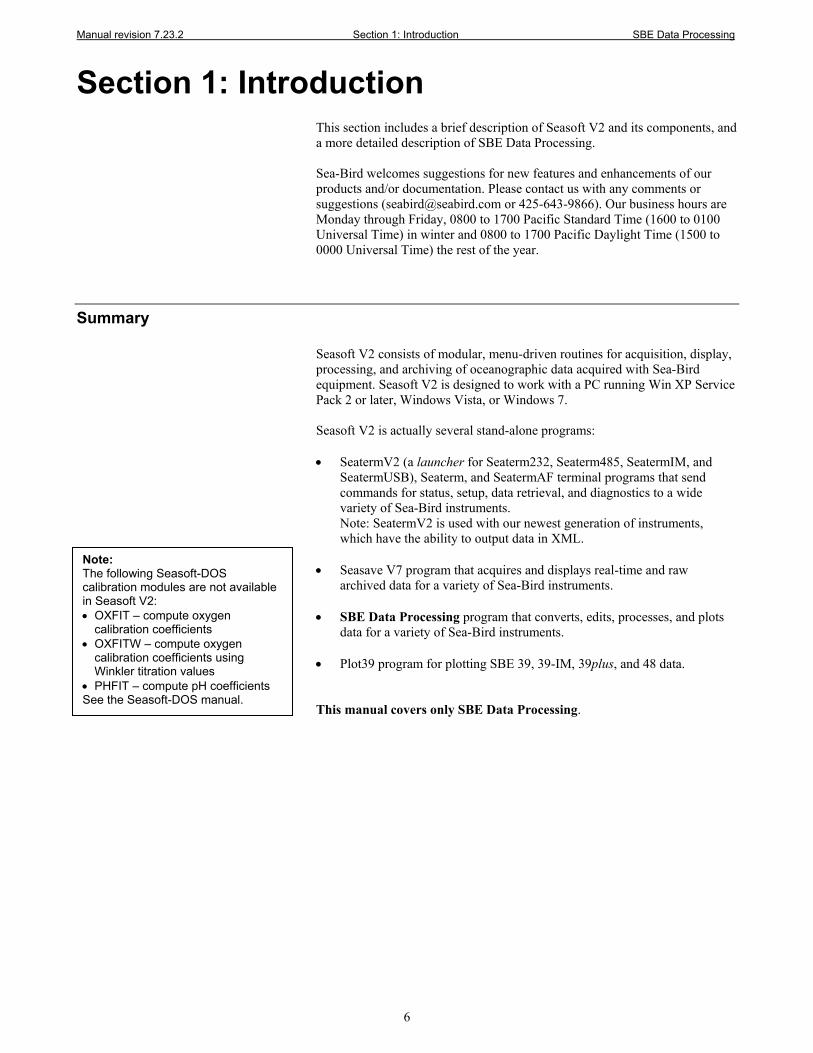
Section 1: Introduction This section includes a brief description of Seasoft V2 and its components, and a more detailed description of SBE Data Processing. Sea-Bird welcomes suggestions for new features and enhancements of our products and/or documentation. Please contact us with any comments or suggestions ([email protected] or 425-643-9866). Our business hours are Monday through Friday, 0800 to 1700 Pacific Standard Time (1600 to 0100 Universal Time) in winter and 0800 to 1700 Pacific Daylight Time (1500 to 0000 Universal Time) the rest of the year.
Summary Seasoft V2 consists of modular, menu-driven routines for acquisition, display, processing, and archiving of oceanographic data acquired with Sea-Bird equipment. Seasoft V2 is designed to work with a PC running Win XP Service Pack 2 or later, Windows Vista, or Windows 7. Seasoft V2 is actually several stand-alone programs: • SeatermV2 (a launcher for Seaterm232, Seaterm485, SeatermIM, and
SeatermUSB), Seaterm, and SeatermAF terminal programs that send commands for status, setup, data retrieval, and diagnostics to a wide variety of Sea-Bird instruments. Note: SeatermV2 is used with our newest generation of instruments, which have the ability to output data in XML.
• Seasave V7 program that acquires and displays real-time and raw
archived data for a variety of Sea-Bird instruments. • SBE Data Processing program that converts, edits, processes, and plots
data for a variety of Sea-Bird instruments. • Plot39 program for plotting SBE 39, 39-IM, 39plus, and 48 data. This manual covers only SBE Data Processing.
Note: The following Seasoft-DOS calibration modules are not available in Seasoft V2: • OXFIT – compute oxygen
calibration coefficients • OXFITW – compute oxygen
calibration coefficients using Winkler titration values
• PHFIT – compute pH coefficients See the Seasoft-DOS manual.
Manual revision 7.23.2 Section 1: Introduction SBE Data Processing
7
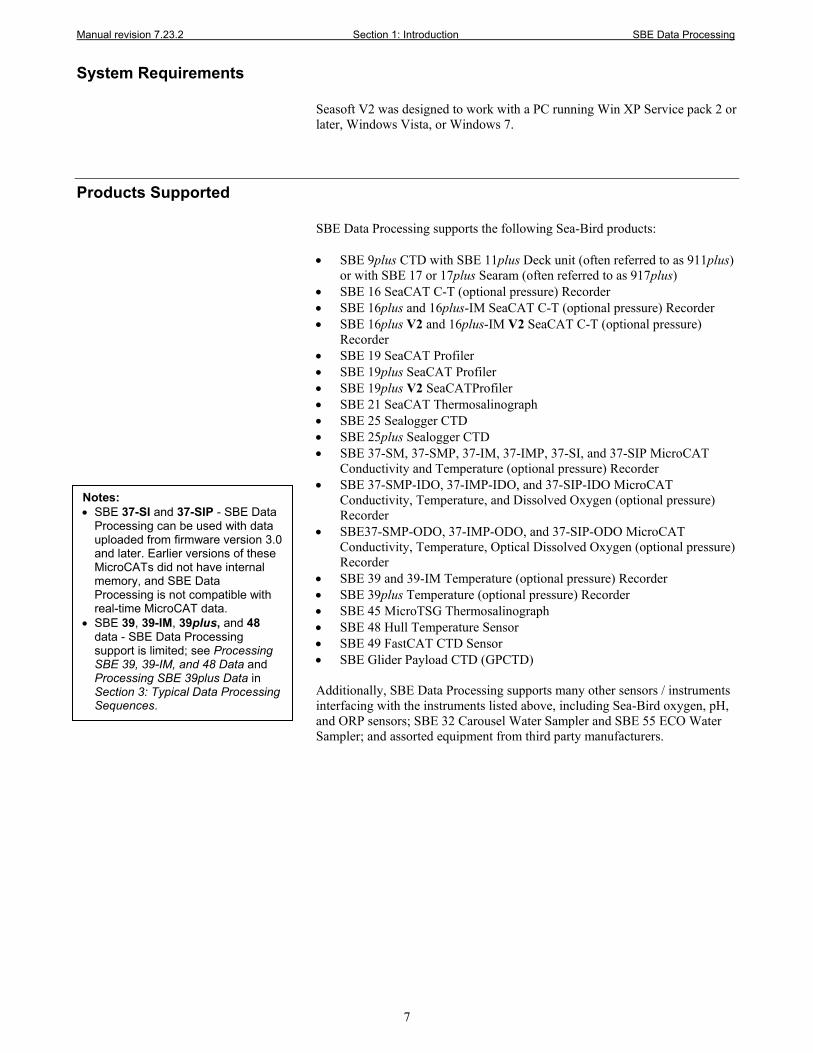
System Requirements Seasoft V2 was designed to work with a PC running Win XP Service pack 2 or later, Windows Vista, or Windows 7.
Products Supported SBE Data Processing supports the following Sea-Bird products: • SBE 9plus CTD with SBE 11plus Deck unit (often referred to as 911plus)
or with SBE 17 or 17plus Searam (often referred to as 917plus) • SBE 16 SeaCAT C-T (optional pressure) Recorder • SBE 16plus and 16plus-IM SeaCAT C-T (optional pressure) Recorder • SBE 16plus V2 and 16plus-IM V2 SeaCAT C-T (optional pressure)
Recorder • SBE 19 SeaCAT Profiler • SBE 19plus SeaCAT Profiler • SBE 19plus V2 SeaCATProfiler • SBE 21 SeaCAT Thermosalinograph • SBE 25 Sealogger CTD • SBE 25plus Sealogger CTD • SBE 37-SM, 37-SMP, 37-IM, 37-IMP, 37-SI, and 37-SIP MicroCAT
Conductivity and Temperature (optional pressure) Recorder • SBE 37-SMP-IDO, 37-IMP-IDO, and 37-SIP-IDO MicroCAT
Conductivity, Temperature, and Dissolved Oxygen (optional pressure) Recorder
• SBE37-SMP-ODO, 37-IMP-ODO, and 37-SIP-ODO MicroCAT Conductivity, Temperature, Optical Dissolved Oxygen (optional pressure) Recorder
• SBE 39 and 39-IM Temperature (optional pressure) Recorder • SBE 39plus Temperature (optional pressure) Recorder • SBE 45 MicroTSG Thermosalinograph • SBE 48 Hull Temperature Sensor • SBE 49 FastCAT CTD Sensor • SBE Glider Payload CTD (GPCTD) Additionally, SBE Data Processing supports many other sensors / instruments interfacing with the instruments listed above, including Sea-Bird oxygen, pH, and ORP sensors; SBE 32 Carousel Water Sampler and SBE 55 ECO Water Sampler; and assorted equipment from third party manufacturers.
Notes: • SBE 37-SI and 37-SIP - SBE Data
Processing can be used with data uploaded from firmware version 3.0 and later. Earlier versions of these MicroCATs did not have internal memory, and SBE Data Processing is not compatible with real-time MicroCAT data.
• SBE 39, 39-IM, 39plus, and 48 data - SBE Data Processing support is limited; see Processing SBE 39, 39-IM, and 48 Data and Processing SBE 39plus Data in Section 3: Typical Data Processing Sequences.
Manual revision 7.23.2 Section 1: Introduction SBE Data Processing
8
Software Modules
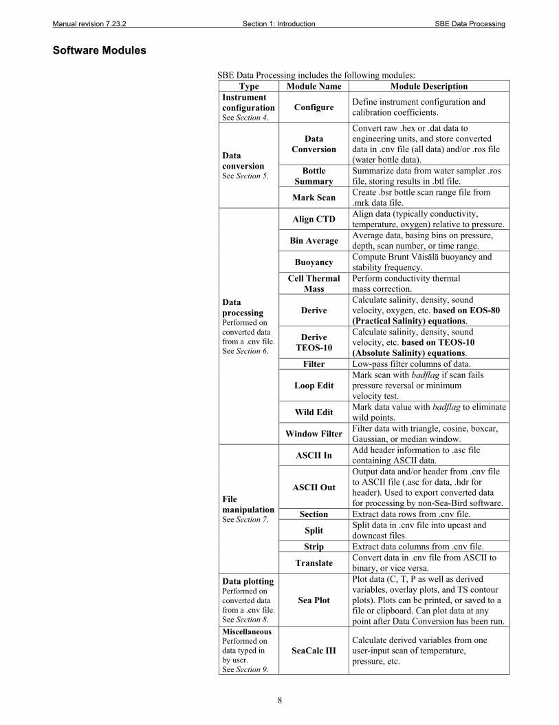
SBE Data Processing includes the following modules: Type Module Name Module Description
Instrument configuration See Section 4.
Configure Define instrument configuration and calibration coefficients.
Data conversion See Section 5.
Data Conversion
Convert raw .hex or .dat data to engineering units, and store converted data in .cnv file (all data) and/or .ros file (water bottle data).
Bottle Summary
Summarize data from water sampler .ros file, storing results in .btl file.
Mark Scan Create .bsr bottle scan range file from .mrk data file.
Data processing Performed on converted data from a .cnv file. See Section 6.
Align CTD Align data (typically conductivity, temperature, oxygen) relative to pressure.
Bin Average Average data, basing bins on pressure, depth, scan number, or time range.
Buoyancy Compute Brunt Väisälä buoyancy and stability frequency.
Cell Thermal Mass
Perform conductivity thermal mass correction.
Derive Calculate salinity, density, sound velocity, oxygen, etc. based on EOS-80 (Practical Salinity) equations.
Derive TEOS-10
Calculate salinity, density, sound velocity, etc. based on TEOS-10 (Absolute Salinity) equations.
Filter Low-pass filter columns of data.
Loop Edit Mark scan with badflag if scan fails pressure reversal or minimum velocity test.
Wild Edit Mark data value with badflag to eliminate wild points.
Window Filter Filter data with triangle, cosine, boxcar, Gaussian, or median window.
File manipulation See Section 7.
ASCII In Add header information to .asc file containing ASCII data.
ASCII Out
Output data and/or header from .cnv file to ASCII file (.asc for data, .hdr for header). Used to export converted data for processing by non-Sea-Bird software.
Section Extract data rows from .cnv file.
Split Split data in .cnv file into upcast and downcast files.
Strip Extract data columns from .cnv file.
Translate Convert data in .cnv file from ASCII to binary, or vice versa.
Data plotting Performed on converted data from a .cnv file. See Section 8.
Sea Plot
Plot data (C, T, P as well as derived variables, overlay plots, and TS contour plots). Plots can be printed, or saved to a file or clipboard. Can plot data at any point after Data Conversion has been run.
Miscellaneous Performed on data typed in by user. See Section 9.
SeaCalc III Calculate derived variables from one user-input scan of temperature, pressure, etc.
Manual revision 7.23.2 Section 2: Installation and Use SBE Data Processing
9
Section 2: Installation and Use Seasoft V2 was designed to work with a PC running Win XP Service pack 2 or later, Windows Vista, or Windows 7.
Installation
If not already installed, install SBE Data Processing and other Sea-Bird software programs on your computer using the supplied software CD: 1. Insert the CD in your CD drive. 2. Double click on SeasoftV2_date.exe (where date is the date the software
release was created). 3. Follow the dialog box directions to install the software.
The default location for the software is c:\Program Files\Sea-Bird. Within that folder is a sub-directory for each program. The installation program allows you to install the desired components. Install all the components, or just install SBE Data Processing. Note that the following additional software is installed with SBE Data Processing, in the same directory as SBE Data Processing: • StripNullChars.exe – This program removes null characters from an
uploaded SBE 25plus data file; the file can then be processed in SBE Data Processing’s Data Conversion module. Run StripNullChars.exe from a DOS window, following instructions
provided in the software. Note that the null characters in the file also prevent uploading of the
data from the SBE 25plus via RS-232. You must open the 25plus and upload via the internal USB connector.
• NMEATest.exe – This program simulates a NMEA navigation device; see the manual for your deck unit (SBE 11plus, 33, or 36 Deck Unit).
• phFit.exe – This program calculates a new offset and slope for a pH sensor; see Application Note 18-1 (www.seabird.com/application_notes/AN18_1.htm).
Note: Sea-Bird supplies the current version of our software when you purchase an instrument. As software revisions occur, we post the revised software on our FTP site. • You may not need the latest
version. Our revisions often include improvements and new features related to one instrument, which may have little or no impact on your operation.
See our website (www.seabird.com) for the latest software version number, a description of the software changes, and instructions for downloading the software from the FTP site.
Manual revision 7.23.2 Section 2: Installation and Use SBE Data Processing
10
Getting Started
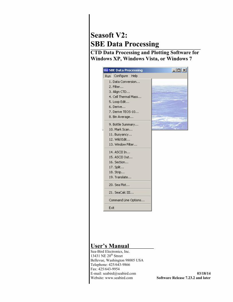
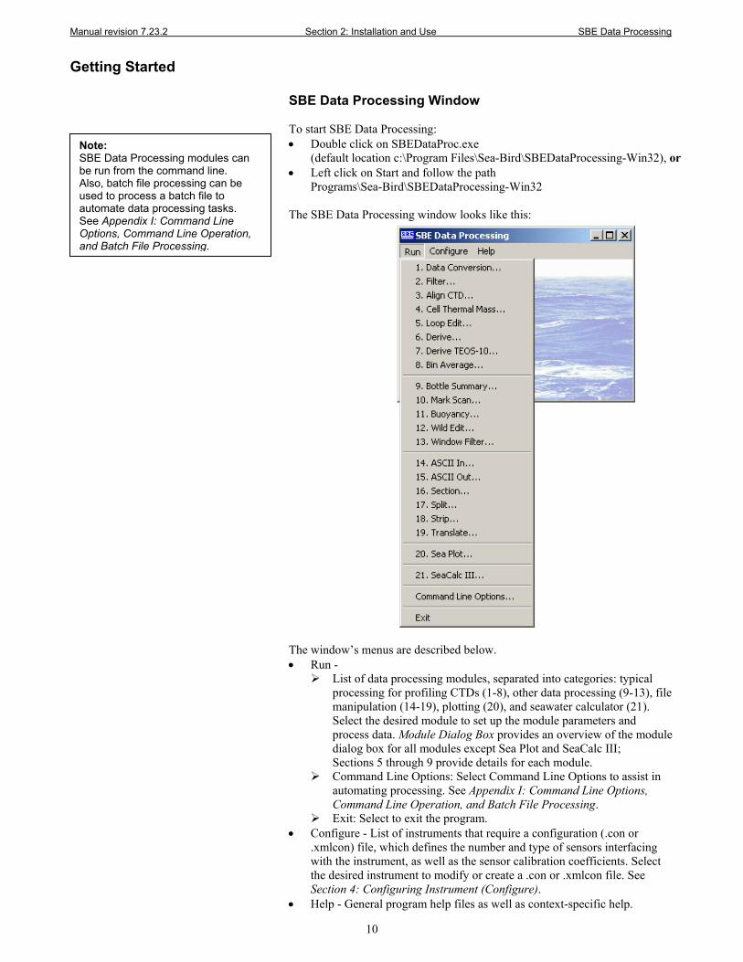
SBE Data Processing Window
To start SBE Data Processing: • Double click on SBEDataProc.exe
(default location c:\Program Files\Sea-Bird\SBEDataProcessing-Win32), or • Left click on Start and follow the path
Programs\Sea-Bird\SBEDataProcessing-Win32 The SBE Data Processing window looks like this:
The window’s menus are described below. • Run -
List of data processing modules, separated into categories: typical processing for profiling CTDs (1-8), other data processing (9-13), file manipulation (14-19), plotting (20), and seawater calculator (21). Select the desired module to set up the module parameters and process data. Module Dialog Box provides an overview of the module dialog box for all modules except Sea Plot and SeaCalc III; Sections 5 through 9 provide details for each module.
Command Line Options: Select Command Line Options to assist in automating processing. See Appendix I: Command Line Options, Command Line Operation, and Batch File Processing.
Exit: Select to exit the program. • Configure - List of instruments that require a configuration (.con or
.xmlcon) file, which defines the number and type of sensors interfacing with the instrument, as well as the sensor calibration coefficients. Select the desired instrument to modify or create a .con or .xmlcon file. See Section 4: Configuring Instrument (Configure).
• Help - General program help files as well as context-specific help.
Note: SBE Data Processing modules can be run from the command line. Also, batch file processing can be used to process a batch file to automate data processing tasks. See Appendix I: Command Line Options, Command Line Operation, and Batch File Processing.
Manual revision 7.23.2 Section 2: Installation and Use SBE Data Processing
11
Module Dialog Box
To open a module, select it in the Run menu of the SBE Data Processing window. Each module’s dialog box has three menus: • File –
Start Process - begin to process data as defined in dialog box
Open - select a different program setup (.psa) file
Save or Save As - save all current settings to a .psa file
Restore - reset all settings to match last saved .psa file
Default File Setup - reset all settings on File Setup tab to defaults
Default Data Setup - reset all settings on Data Setup tab to defaults
Exit or Save & Exit - exit module and return to SBE Data Processing window
• Options (where applicable) –
Confirm Program Setup Change - - If selected, program provides a prompt to save the program setup (.psa) file if you make changes and click the Exit button or select Exit in the File menu without clicking or selecting Save or Save As. - If not selected, program changes Exit to Save & Exit; to exit without saving changes, use the Cancel button.
Confirm Instrument Configuration Change -
- If selected, program provides a prompt to save the configuration (.con or .xmlcon) file if you make changes and then click the Exit button in the Configuration dialog box without clicking Save or Save As. - If not selected, program changes Exit button to Save & Exit; to exit without saving changes, use the Cancel button.
Overwrite Output File Warning -
- If selected, program provides a warning if output data will overwrite an existing file. - If not selected, program automatically overwrites an existing file with the same file name as the output file.
Inconsistent Data Setup Warning -
- If selected, program provides a warning if the configuration (.con or .xmlcon) file and/or the input data file are inconsistent with the selected output variables. For example, if the user-selected output variables include conductivity difference, but you remove the second conductivity sensor from the configuration file, a warning will appear. The warning details what output variable cannot be calculated, and allows you to retain the change to the configuration file (and remove the inconsistent output variable) or restore the configuration file to the previous configuration. - If not selected, program automatically changes the user-selected output variables to be consistent with the selected configuration or data file.
Manual revision 7.23.2 Section 2: Installation and Use SBE Data Processing
12
Sort Input Files (applicable only to Sea Plot) –
- If selected, Sea Plot sorts the input files in alphabetical order. - If not selected, Sea Plot maintains the order of the files as you selected them using the Ctrl key; use this feature if there is a particular data set you want to use as the base on a waterfall overlay plot. Note that using the Shift key to select files will not maintain the selected order.
Diagnostics log – If selected, brings up a Diagnostics dialog box.
- Select Keep a diagnostics log to enable diagnostics output. - Click Select Path to select the location and name for the diagnostics file. The default location is %USERPROFILE%\Application Data\ Sea-Bird; the default name is PostProcLog.txt (Example c:\Documents and Settings\dbresko\Application Data\ Sea-Bird\PostProcLog.txt). - Select the Level of diagnostics to include: Errors, Warnings (includes Errors), or Information (includes Errors and Warnings). - If desired, click Display Log File to display the contents of the indicated file, using Notepad. - If desired, click Erase Log File to erase the contents of the indicated file. If not erased, SBE Data Processing appends diagnostics data to the end of the file. - Click OK.
• Help - contains general program help files as well as context-specific help
(where applicable) Each module’s dialog box typically has three tabs - File Setup, Data Setup, and Header View. The File Setup and Header View tabs are similar for most modules, and are discussed below. The Data Setup tab contains input parameters specific to the module. Additionally, Data Conversion and Derive have a fourth tab – Miscellaneous. See the module discussions in Sections 5 through 7 for details.
Note: The dialog box for Sea Plot and SeaCalc III differ from the other modules. See Section 8: Data Plotting Module – Sea Plot and Section 9: Miscellaneous Module – SeaCalc III.
Manual revision 7.23.2 Section 2: Installation and Use SBE Data Processing
13
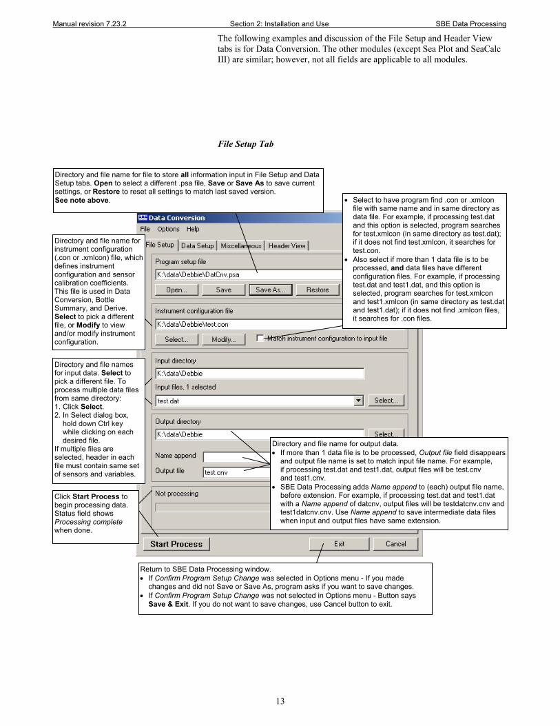
The following examples and discussion of the File Setup and Header View tabs is for Data Conversion. The other modules (except Sea Plot and SeaCalc III) are similar; however, not all fields are applicable to all modules. File Setup Tab
Directory and file name for instrument configuration (.con or .xmlcon) file, which defines instrument configuration and sensor calibration coefficients. This file is used in Data Conversion, Bottle Summary, and Derive. Select to pick a different file, or Modify to view and/or modify instrument configuration.
• Select to have program find .con or .xmlcon file with same name and in same directory as data file. For example, if processing test.dat and this option is selected, program searches for test.xmlcon (in same directory as test.dat); if it does not find test.xmlcon, it searches for test.con.
• Also select if more than 1 data file is to be processed, and data files have different configuration files. For example, if processing test.dat and test1.dat, and this option is selected, program searches for test.xmlcon and test1.xmlcon (in same directory as test.dat and test1.dat); if it does not find .xmlcon files, it searches for .con files.
Directory and file names for input data. Select to pick a different file. To process multiple data files from same directory: 1. Click Select. 2. In Select dialog box,
hold down Ctrl key while clicking on each desired file.
If multiple files are selected, header in each file must contain same set of sensors and variables.
Directory and file name for output data. • If more than 1 data file is to be processed, Output file field disappears
and output file name is set to match input file name. For example, if processing test.dat and test1.dat, output files will be test.cnv and test1.cnv.
• SBE Data Processing adds Name append to (each) output file name, before extension. For example, if processing test.dat and test1.dat with a Name append of datcnv, output files will be testdatcnv.cnv and test1datcnv.cnv. Use Name append to save intermediate data files when input and output files have same extension.
Click Start Process to begin processing data. Status field shows Processing complete when done.
Return to SBE Data Processing window. • If Confirm Program Setup Change was selected in Options menu - If you made
changes and did not Save or Save As, program asks if you want to save changes. • If Confirm Program Setup Change was not selected in Options menu - Button says
Save & Exit. If you do not want to save changes, use Cancel button to exit.
Directory and file name for file to store all information input in File Setup and Data Setup tabs. Open to select a different .psa file, Save or Save As to save current settings, or Restore to reset all settings to match last saved version. See note above.
Manual revision 7.23.2 Section 2: Installation and Use SBE Data Processing
14
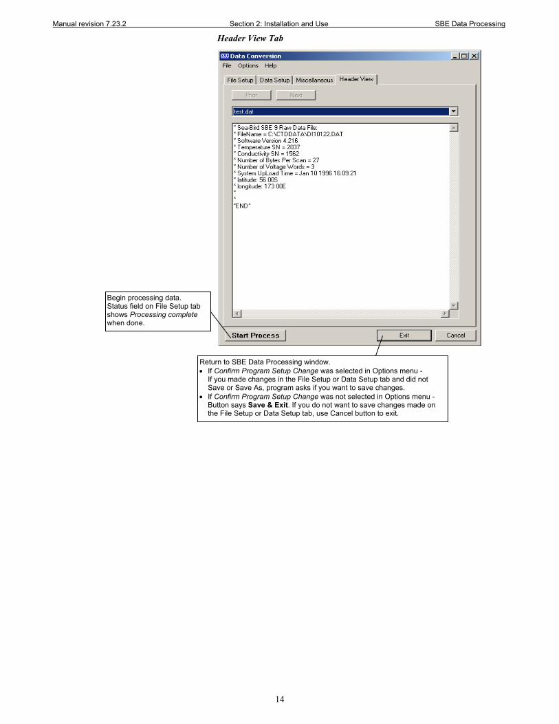
Header View Tab
Return to SBE Data Processing window. • If Confirm Program Setup Change was selected in Options menu -
If you made changes in the File Setup or Data Setup tab and did not Save or Save As, program asks if you want to save changes.
• If Confirm Program Setup Change was not selected in Options menu - Button says Save & Exit. If you do not want to save changes made on the File Setup or Data Setup tab, use Cancel button to exit.
Begin processing data. Status field on File Setup tab shows Processing complete when done.
Manual revision 7.23.2 Section 2: Installation and Use SBE Data Processing
15
File Formats
File extensions are used by Seasoft to indicate the file type: Extension Description
.afm Bottle sequence, date and time, firing confirmation, and 5 scans of CTD data, created by Auto Fire Module (AFM) or (when used for autonomous operation) SBE 55 ECO Water Sampler.
.asc
Data file: • Data portion of .cnv converted data file written in ASCII by
ASCII Out • File written by Seaterm for data uploaded from SBE 37
(firmware < 3.0), 39, 39-IM, or 48. Notes: 1. Convert button on Seaterm’s toolbar can convert .asc file to .cnv file that can be used by SBE Data Processing to process data. 2. Not applicable to SBE 37 IDO or ODO MicroCATs.
• File written by SeatermV2 for data uploaded from SBE 39plus.
.bl
Bottle log information - output bottle file, containing bottle firing sequence number and position, date, time, and beginning and ending scan numbers for each bottle closure. Beginning and ending scan numbers correspond to approximately 1.5-second duration for each bottle. Seasave writes information to file each time bottle fire confirmation is received from SBE 32 Carousel Water Sampler or SBE 55 ECO Water Sampler or (only when used with SBE 911plus) G.O. 1016 Rosette. File can be used by Data Conversion.
.bmp Sea Plot output bitmap graphics file.
.bsr Bottle scan range file created by Mark Scan, and used by Data Conversion to create a .ros file.
.btl Averaged and derived bottle data from .ros file, created by Bottle Summary.
.cnv
Converted (engineering units) data file, with ASCII header preceding data. Created by: • Data Conversion. • SeatermV2’s Convert XML data file (in Tools menu) for
SBE 39plus. • Upload menu in Seaterm232 (SBE Glider Payload CTD only) • Seaterm’s Convert button (SBE 37 [firmware < 3.0], 39,
39-IM, or 48 only). Note: Not applicable to SBE 37 IDO or ODO MicroCATs.
.con or .xmlcon
Instrument configuration - number and type of sensors, channel assigned to each sensor, and calibration coefficients. SBE Data Processing uses this information to interpret raw data from instrument. Latest version of configuration file for your instrument is supplied by Sea-Bird when instrument is purchased, upgraded, or calibrated. If you make changes to instrument (add or remove sensors, recalibrate, etc.), you must update configuration file. Can be viewed and/or modified in SBE Data Processing in Configure, Data Conversion, Derive, and Bottle Summary; and in Seasave. • .xmlcon files, written in XML format, were introduced with
SBE Data Processing and Seasave 7.20a. Instruments introduced after that are compatible only with .xmlcon files.
.dat Data file - binary raw data file created by older versions (Version < 6.0) of Seasave from real-time data stream from SBE 911plus. File includes header information.
Notes: • Configuration files (.con or .xmlcon)
can also be opened, viewed, and modified with DisplayConFile.exe, a utility that is installed in the same folder as SBE Data Processing. Right click on the desired configuration file, select Open With, and select DisplayConFile. This utility is often used at Sea-Bird to quickly open and view a configuration file for troubleshooting purposes, without needing to go through the additional steps of selecting the file in SBE Data Processing or Seasave.
• We recommend that you do not open .xmlcon files with a text editor (i.e., Notepad, Wordpad, etc.).
Manual revision 7.23.2 Section 2: Installation and Use SBE Data Processing
16
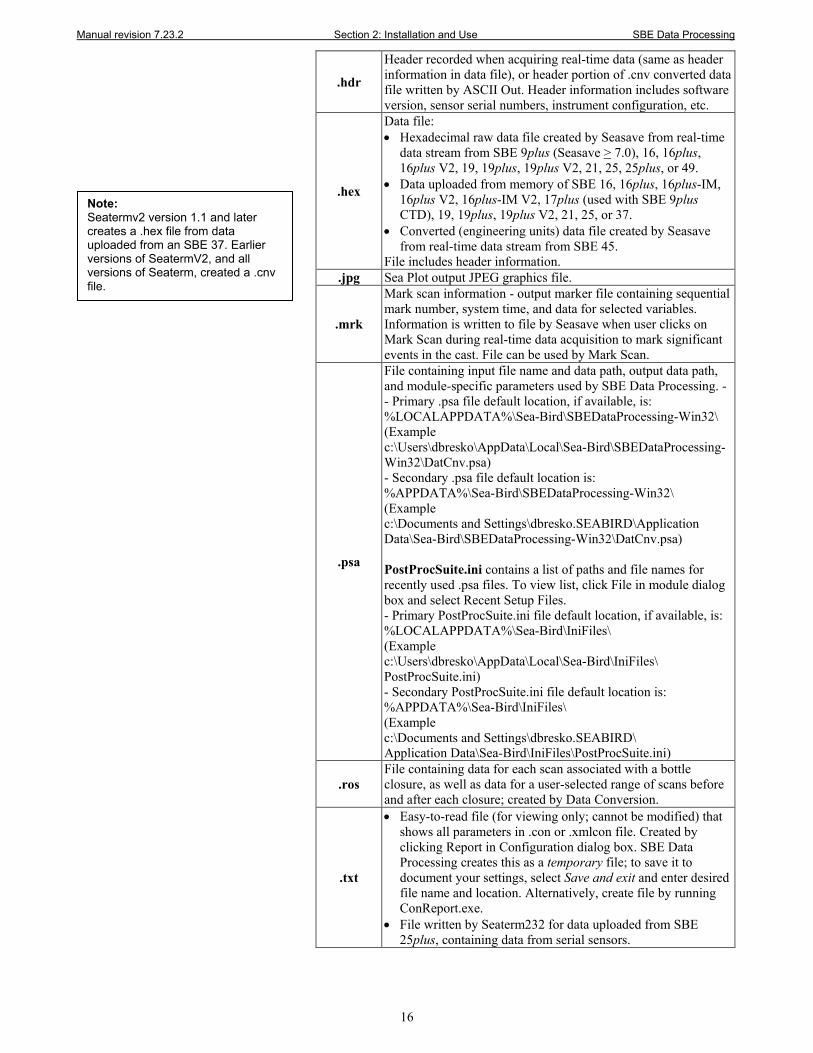
.hdr
Header recorded when acquiring real-time data (same as header information in data file), or header portion of .cnv converted data file written by ASCII Out. Header information includes software version, sensor serial numbers, instrument configuration, etc.
.hex
Data file: • Hexadecimal raw data file created by Seasave from real-time
data stream from SBE 9plus (Seasave > 7.0), 16, 16plus, 16plus V2, 19, 19plus, 19plus V2, 21, 25, 25plus, or 49.
• Data uploaded from memory of SBE 16, 16plus, 16plus-IM, 16plus V2, 16plus-IM V2, 17plus (used with SBE 9plus CTD), 19, 19plus, 19plus V2, 21, 25, or 37.
• Converted (engineering units) data file created by Seasave from real-time data stream from SBE 45.
File includes header information. .jpg Sea Plot output JPEG graphics file.
.mrk
Mark scan information - output marker file containing sequential mark number, system time, and data for selected variables. Information is written to file by Seasave when user clicks on Mark Scan during real-time data acquisition to mark significant events in the cast. File can be used by Mark Scan.
.psa
File containing input file name and data path, output data path, and module-specific parameters used by SBE Data Processing. - - Primary .psa file default location, if available, is: %LOCALAPPDATA%\Sea-Bird\SBEDataProcessing-Win32\ (Example c:\Users\dbresko\AppData\Local\Sea-Bird\SBEDataProcessing-Win32\DatCnv.psa) - Secondary .psa file default location is: %APPDATA%\Sea-Bird\SBEDataProcessing-Win32\ (Example c:\Documents and Settings\dbresko.SEABIRD\Application Data\Sea-Bird\SBEDataProcessing-Win32\DatCnv.psa) PostProcSuite.ini contains a list of paths and file names for recently used .psa files. To view list, click File in module dialog box and select Recent Setup Files. - Primary PostProcSuite.ini file default location, if available, is: %LOCALAPPDATA%\Sea-Bird\IniFiles\ (Example c:\Users\dbresko\AppData\Local\Sea-Bird\IniFiles\ PostProcSuite.ini) - Secondary PostProcSuite.ini file default location is: %APPDATA%\Sea-Bird\IniFiles\ (Example c:\Documents and Settings\dbresko.SEABIRD\ Application Data\Sea-Bird\IniFiles\PostProcSuite.ini)
.ros File containing data for each scan associated with a bottle closure, as well as data for a user-selected range of scans before and after each closure; created by Data Conversion.
.txt
• Easy-to-read file (for viewing only; cannot be modified) that shows all parameters in .con or .xmlcon file. Created by clicking Report in Configuration dialog box. SBE Data Processing creates this as a temporary file; to save it to document your settings, select Save and exit and enter desired file name and location. Alternatively, create file by running ConReport.exe.
• File written by Seaterm232 for data uploaded from SBE 25plus, containing data from serial sensors.
Note: Seatermv2 version 1.1 and later creates a .hex file from data uploaded from an SBE 37. Earlier versions of SeatermV2, and all versions of Seaterm, created a .cnv file.
Manual revision 7.23.2 Section 2: Installation and Use SBE Data Processing
17
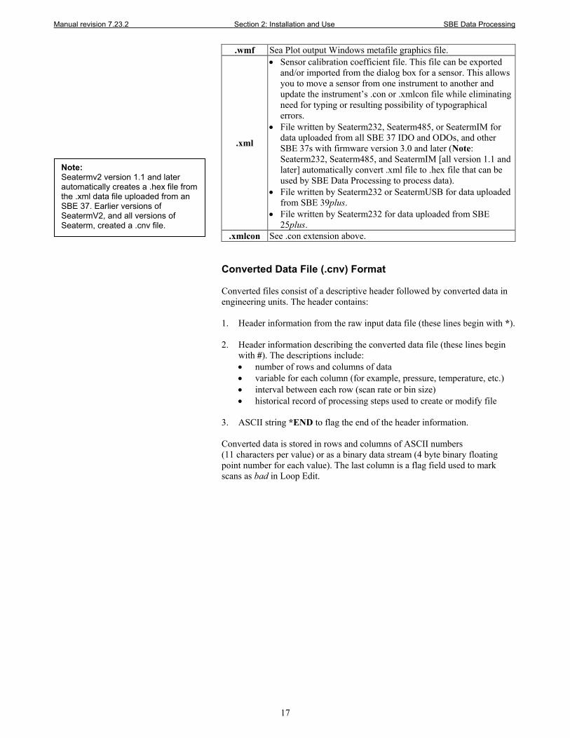
.wmf Sea Plot output Windows metafile graphics file.
.xml
• Sensor calibration coefficient file. This file can be exported and/or imported from the dialog box for a sensor. This allows you to move a sensor from one instrument to another and update the instrument’s .con or .xmlcon file while eliminating need for typing or resulting possibility of typographical errors.
• File written by Seaterm232, Seaterm485, or SeatermIM for data uploaded from all SBE 37 IDO and ODOs, and other SBE 37s with firmware version 3.0 and later (Note: Seaterm232, Seaterm485, and SeatermIM [all version 1.1 and later] automatically convert .xml file to .hex file that can be used by SBE Data Processing to process data).
• File written by Seaterm232 or SeatermUSB for data uploaded from SBE 39plus.
• File written by Seaterm232 for data uploaded from SBE 25plus.
.xmlcon See .con extension above.
Converted Data File (.cnv) Format Converted files consist of a descriptive header followed by converted data in engineering units. The header contains: 1. Header information from the raw input data file (these lines begin with *). 2. Header information describing the converted data file (these lines begin
with #). The descriptions include: • number of rows and columns of data • variable for each column (for example, pressure, temperature, etc.) • interval between each row (scan rate or bin size) • historical record of processing steps used to create or modify file
3. ASCII string *END to flag the end of the header information. Converted data is stored in rows and columns of ASCII numbers (11 characters per value) or as a binary data stream (4 byte binary floating point number for each value). The last column is a flag field used to mark scans as bad in Loop Edit.
Note: Seatermv2 version 1.1 and later automatically creates a .hex file from the .xml data file uploaded from an SBE 37. Earlier versions of SeatermV2, and all versions of Seaterm, created a .cnv file.
Manual revision 7.23.2 Section 2: Installation and Use SBE Data Processing
18
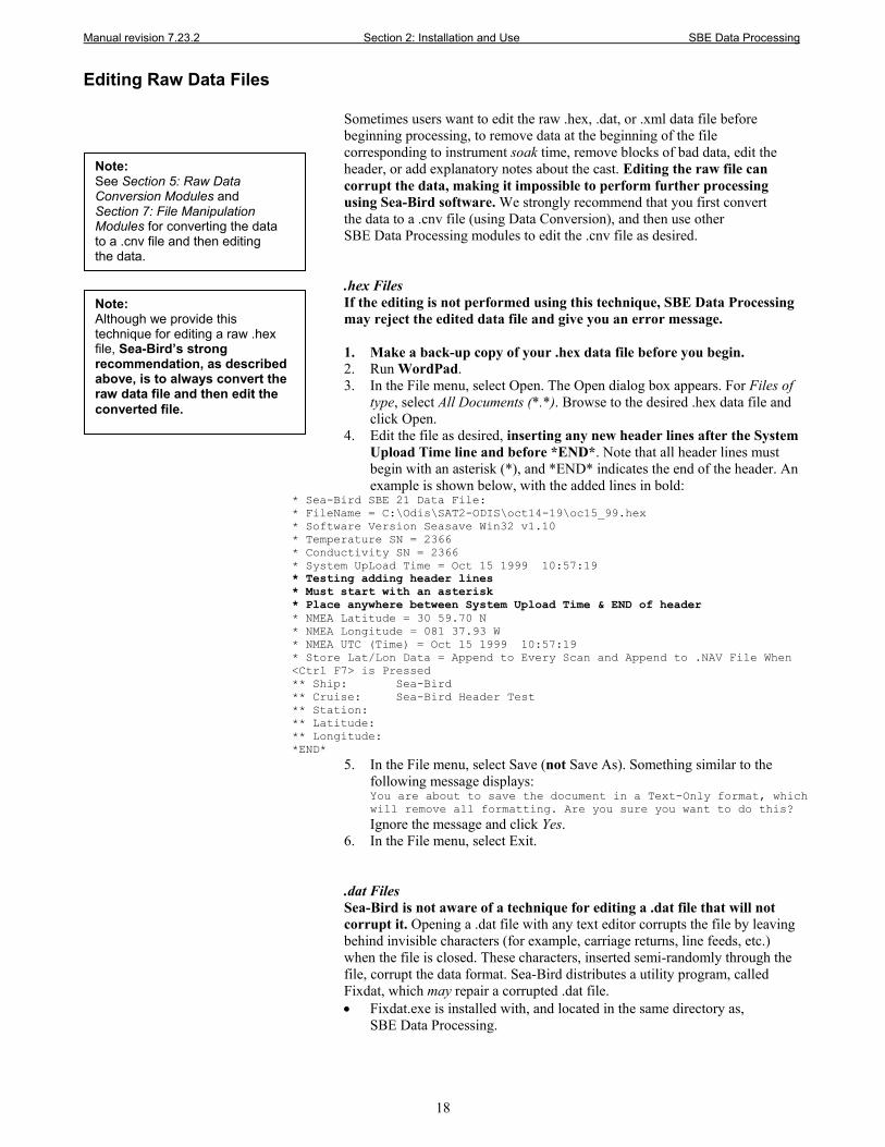
Editing Raw Data Files Sometimes users want to edit the raw .hex, .dat, or .xml data file before beginning processing, to remove data at the beginning of the file corresponding to instrument soak time, remove blocks of bad data, edit the header, or add explanatory notes about the cast. Editing the raw file can corrupt the data, making it impossible to perform further processing using Sea-Bird software. We strongly recommend that you first convert the data to a .cnv file (using Data Conversion), and then use other SBE Data Processing modules to edit the .cnv file as desired. .hex Files If the editing is not performed using this technique, SBE Data Processing may reject the edited data file and give you an error message. 1. Make a back-up copy of your .hex data file before you begin. 2. Run WordPad. 3. In the File menu, select Open. The Open dialog box appears. For Files of
type, select All Documents (*.*). Browse to the desired .hex data file and click Open.
4. Edit the file as desired, inserting any new header lines after the System Upload Time line and before *END*. Note that all header lines must begin with an asterisk (*), and *END* indicates the end of the header. An example is shown below, with the added lines in bold:
* Sea-Bird SBE 21 Data File: * FileName = C:\Odis\SAT2-ODIS\oct14-19\oc15_99.hex * Software Version Seasave Win32 v1.10 * Temperature SN = 2366 * Conductivity SN = 2366 * System UpLoad Time = Oct 15 1999 10:57:19 * Testing adding header lines * Must start with an asterisk * Place anywhere between System Upload Time & END of header * NMEA Latitude = 30 59.70 N * NMEA Longitude = 081 37.93 W * NMEA UTC (Time) = Oct 15 1999 10:57:19 * Store Lat/Lon Data = Append to Every Scan and Append to .NAV File When <Ctrl F7> is Pressed ** Ship: Sea-Bird ** Cruise: Sea-Bird Header Test ** Station: ** Latitude: ** Longitude: *END*
5. In the File menu, select Save (not Save As). Something similar to the following message displays: You are about to save the document in a Text-Only format, which will remove all formatting. Are you sure you want to do this? Ignore the message and click Yes.
6. In the File menu, select Exit.
.dat Files Sea-Bird is not aware of a technique for editing a .dat file that will not corrupt it. Opening a .dat file with any text editor corrupts the file by leaving behind invisible characters (for example, carriage returns, line feeds, etc.) when the file is closed. These characters, inserted semi-randomly through the file, corrupt the data format. Sea-Bird distributes a utility program, called Fixdat, which may repair a corrupted .dat file. • Fixdat.exe is installed with, and located in the same directory as,
SBE Data Processing.
Note: See Section 5: Raw Data Conversion Modules and Section 7: File Manipulation Modules for converting the data to a .cnv file and then editing the data.
Note: Although we provide this technique for editing a raw .hex file, Sea-Bird’s strong recommendation, as described above, is to always convert the raw data file and then edit the converted file.
Manual revision 7.23.2 Section 3: Typical Data Processing Sequences SBE Data Processing
19
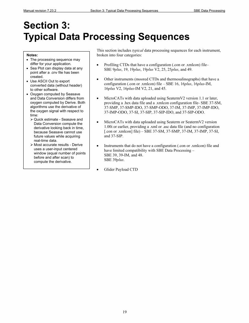
Section 3: Typical Data Processing Sequences
This section includes typical data processing sequences for each instrument, broken into four categories: • Profiling CTDs that have a configuration (.con or .xmlcon) file–
SBE 9plus, 19, 19plus, 19plus V2, 25, 25plus, and 49. • Other instruments (moored CTDs and thermosalinographs) that have a
configuration (.con or .xmlcon) file – SBE 16, 16plus, 16plus-IM, 16plus V2, 16plus-IM V2, 21, and 45.
• MicroCATs with data uploaded using SeatermV2 version 1.1 or later,
providing a .hex data file and a .xmlcon configuration file- SBE 37-SM, 37-SMP, 37-SMP-IDO, 37-SMP-ODO, 37-IM, 37-IMP, 37-IMP-IDO, 37-IMP-ODO, 37-SI, 37-SIP, 37-SIP-IDO, and 37-SIP-ODO.
• MicroCATs with data uploaded using Seaterm or SeatermV2 version
1.00i or earlier, providing a .xml or .asc data file (and no configuration [.con or .xmlcon] file) – SBE 37-SM, 37-SMP, 37-IM, 37-IMP, 37-SI, and 37-SIP.
• Instruments that do not have a configuration (.con or .xmlcon) file and
have limited compatibility with SBE Data Processing – SBE 39, 39-IM, and 48. SBE 39plus.
• Glider Payload CTD
Notes: • The processing sequence may
differ for your application. • Sea Plot can display data at any
point after a .cnv file has been created.
• Use ASCII Out to export converted data (without header) to other software.
• Oxygen computed by Seasave and Data Conversion differs from oxygen computed by Derive. Both algorithms use the derivative of the oxygen signal with respect to time: Quick estimate - Seasave and
Data Conversion compute the derivative looking back in time, because Seasave cannot use future values while acquiring real-time data.
Most accurate results - Derive uses a user-input centered window (equal number of points before and after scan) to compute the derivative.
Manual revision 7.23.2 Section 3: Typical Data Processing Sequences SBE Data Processing
20
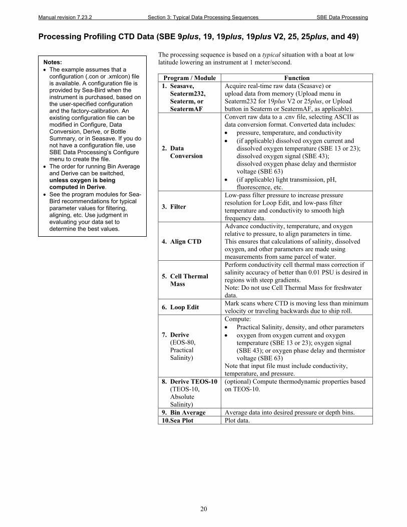
Processing Profiling CTD Data (SBE 9plus, 19, 19plus, 19plus V2, 25, 25plus, and 49)
The processing sequence is based on a typical situation with a boat at low latitude lowering an instrument at 1 meter/second.
Program / Module Function 1. Seasave,
Seaterm232, Seaterm, or SeatermAF
Acquire real-time raw data (Seasave) or upload data from memory (Upload menu in Seaterm232 for 19plus V2 or 25plus, or Upload button in Seaterm or SeatermAF, as applicable).
2. Data Conversion
Convert raw data to a .cnv file, selecting ASCII as data conversion format. Converted data includes: • pressure, temperature, and conductivity • (if applicable) dissolved oxygen current and
dissolved oxygen temperature (SBE 13 or 23); dissolved oxygen signal (SBE 43); dissolved oxygen phase delay and thermistor voltage (SBE 63)
• (if applicable) light transmission, pH, fluorescence, etc.
3. Filter
Low-pass filter pressure to increase pressure resolution for Loop Edit, and low-pass filter temperature and conductivity to smooth high frequency data.
4. Align CTD
Advance conductivity, temperature, and oxygen relative to pressure, to align parameters in time. This ensures that calculations of salinity, dissolved oxygen, and other parameters are made using measurements from same parcel of water.
5. Cell Thermal Mass
Perform conductivity cell thermal mass correction if salinity accuracy of better than 0.01 PSU is desired in regions with steep gradients. Note: Do not use Cell Thermal Mass for freshwater data.
6. Loop Edit Mark scans where CTD is moving less than minimum velocity or traveling backwards due to ship roll.
7. Derive (EOS-80, Practical Salinity)
Compute: • Practical Salinity, density, and other parameters • oxygen from oxygen current and oxygen
temperature (SBE 13 or 23); oxygen signal (SBE 43); or oxygen phase delay and thermistor voltage (SBE 63)
Note that input file must include conductivity, temperature, and pressure.
8. Derive TEOS-10 (TEOS-10, Absolute Salinity)
(optional) Compute thermodynamic properties based on TEOS-10.
9. Bin Average Average data into desired pressure or depth bins. 10. Sea Plot Plot data.
Notes: • The example assumes that a
configuration (.con or .xmlcon) file is available. A configuration file is provided by Sea-Bird when the instrument is purchased, based on the user-specified configuration and the factory-calibration. An existing configuration file can be modified in Configure, Data Conversion, Derive, or Bottle Summary, or in Seasave. If you do not have a configuration file, use SBE Data Processing’s Configure menu to create the file.
• The order for running Bin Average and Derive can be switched, unless oxygen is being computed in Derive.
• See the program modules for Sea-Bird recommendations for typical parameter values for filtering, aligning, etc. Use judgment in evaluating your data set to determine the best values.
Manual revision 7.23.2 Section 3: Typical Data Processing Sequences SBE Data Processing
21
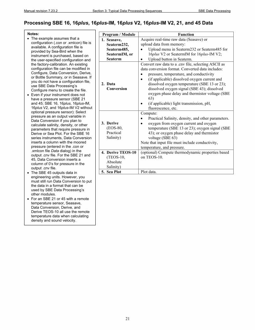
Processing SBE 16, 16plus, 16plus-IM, 16plus V2, 16plus-IM V2, 21, and 45 Data
Program / Module Function 1. Seasave,
Seaterm232, Seaterm485, SeatermIM, or Seaterm
Acquire real-time raw data (Seasave) or upload data from memory: • Upload menu in Seaterm232 or Seaterm485 for
16plus V2 or SeatermIM for 16plus-IM V2; • Upload button in Seaterm.
2. Data Conversion
Convert raw data to a .cnv file, selecting ASCII as data conversion format. Converted data includes: • pressure, temperature, and conductivity • (if applicable) dissolved oxygen current and
dissolved oxygen temperature (SBE 13 or 23); dissolved oxygen signal (SBE 43); dissolved oxygen phase delay and thermistor voltage (SBE 63)
• (if applicable) light transmission, pH, fluorescence, etc.
3. Derive (EOS-80, Practical Salinity)
Compute: • Practical Salinity, density, and other parameters. • oxygen from oxygen current and oxygen
temperature (SBE 13 or 23); oxygen signal (SBE 43); or oxygen phase delay and thermistor voltage (SBE 63)
Note that input file must include conductivity, temperature, and pressure.
4. Derive TEOS-10 (TEOS-10, Absolute Salinity)
(optional) Compute thermodynamic properties based on TEOS-10.
5. Sea Plot Plot data.
Notes: • The example assumes that a
configuration (.con or .xmlcon) file is available. A configuration file is provided by Sea-Bird when the instrument is purchased, based on the user-specified configuration and the factory-calibration. An existing configuration file can be modified in Configure, Data Conversion, Derive, or Bottle Summary, or in Seasave. If you do not have a configuration file, use SBE Data Processing’s Configure menu to create the file.
• Even if your instrument does not have a pressure sensor (SBE 21 and 45; SBE 16, 16plus, 16plus-IM, 16plus V2, and 16plus-IM V2 without optional pressure sensor): Select pressure as an output variable in Data Conversion if you plan to calculate salinity, density, or other parameters that require pressure in Derive or Sea Plot. For the SBE 16 series instruments, Data Conversion inserts a column with the moored pressure (entered in the .con or .xmlcon file Data dialog) in the output .cnv file. For the SBE 21 and 45, Data Conversion inserts a column of 0’s for pressure in the output .cnv file.
• The SBE 45 outputs data in engineering units. However, you must still run Data Conversion to put the data in a format that can be used by SBE Data Processing’s other modules.
• For an SBE 21 or 45 with a remote temperature sensor, Seasave, Data Conversion, Derive, and Derive TEOS-10 all use the remote temperature data when calculating density and sound velocity.
Manual revision 7.23.2 Section 3: Typical Data Processing Sequences SBE Data Processing
22
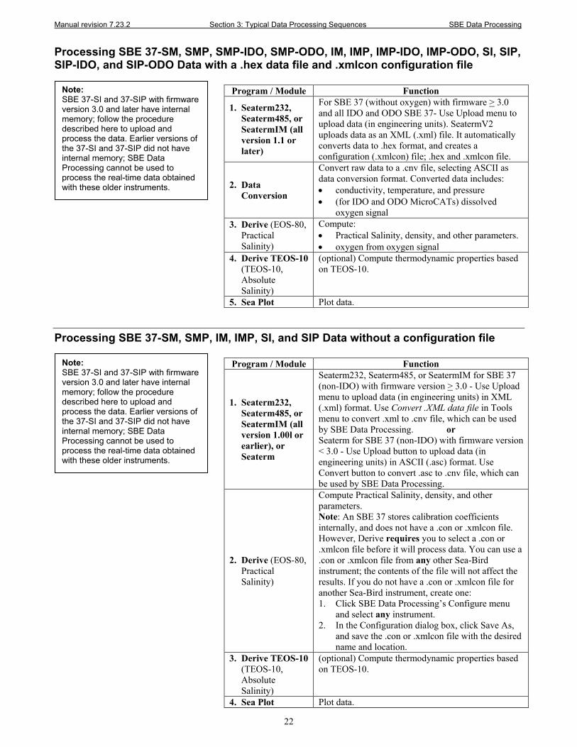
Processing SBE 37-SM, SMP, SMP-IDO, SMP-ODO, IM, IMP, IMP-IDO, IMP-ODO, SI, SIP, SIP-IDO, and SIP-ODO Data with a .hex data file and .xmlcon configuration file
Program / Module Function
1. Seaterm232, Seaterm485, or SeatermIM (all version 1.1 or later)
For SBE 37 (without oxygen) with firmware > 3.0 and all IDO and ODO SBE 37- Use Upload menu to upload data (in engineering units). SeatermV2 uploads data as an XML (.xml) file. It automatically converts data to .hex format, and creates a configuration (.xmlcon) file; .hex and .xmlcon file.
2. Data Conversion
Convert raw data to a .cnv file, selecting ASCII as data conversion format. Converted data includes: • conductivity, temperature, and pressure • (for IDO and ODO MicroCATs) dissolved
oxygen signal 3. Derive (EOS-80,
Practical Salinity)
Compute: • Practical Salinity, density, and other parameters. • oxygen from oxygen signal
4. Derive TEOS-10 (TEOS-10, Absolute Salinity)
(optional) Compute thermodynamic properties based on TEOS-10.
5. Sea Plot Plot data.
Processing SBE 37-SM, SMP, IM, IMP, SI, and SIP Data without a configuration file
Program / Module Function
1. Seaterm232, Seaterm485, or SeatermIM (all version 1.00l or earlier), or Seaterm
Seaterm232, Seaterm485, or SeatermIM for SBE 37 (non-IDO) with firmware version > 3.0 - Use Upload menu to upload data (in engineering units) in XML (.xml) format. Use Convert .XML data file in Tools menu to convert .xml to .cnv file, which can be used by SBE Data Processing. or Seaterm for SBE 37 (non-IDO) with firmware version < 3.0 - Use Upload button to upload data (in engineering units) in ASCII (.asc) format. Use Convert button to convert .asc to .cnv file, which can be used by SBE Data Processing.
2. Derive (EOS-80, Practical Salinity)
Compute Practical Salinity, density, and other parameters. Note: An SBE 37 stores calibration coefficients internally, and does not have a .con or .xmlcon file. However, Derive requires you to select a .con or .xmlcon file before it will process data. You can use a .con or .xmlcon file from any other Sea-Bird instrument; the contents of the file will not affect the results. If you do not have a .con or .xmlcon file for another Sea-Bird instrument, create one: 1. Click SBE Data Processing’s Configure menu
and select any instrument. 2. In the Configuration dialog box, click Save As,
and save the .con or .xmlcon file with the desired name and location.
3. Derive TEOS-10 (TEOS-10, Absolute Salinity)
(optional) Compute thermodynamic properties based on TEOS-10.
4. Sea Plot Plot data.
Note: SBE 37-SI and 37-SIP with firmware version 3.0 and later have internal memory; follow the procedure described here to upload and process the data. Earlier versions of the 37-SI and 37-SIP did not have internal memory; SBE Data Processing cannot be used to process the real-time data obtained with these older instruments.
Note: SBE 37-SI and 37-SIP with firmware version 3.0 and later have internal memory; follow the procedure described here to upload and process the data. Earlier versions of the 37-SI and 37-SIP did not have internal memory; SBE Data Processing cannot be used to process the real-time data obtained with these older instruments.
Manual revision 7.23.2 Section 3: Typical Data Processing Sequences SBE Data Processing
23
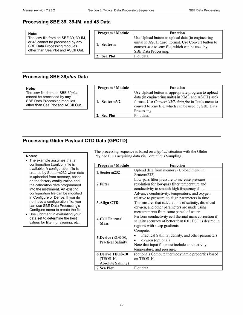
Processing SBE 39, 39-IM, and 48 Data
Program / Module Function
1. Seaterm
Use Upload button to upload data (in engineering units) in ASCII (.asc) format. Use Convert button to convert .asc to .cnv file, which can be used by SBE Data Processing.
2. Sea Plot Plot data.
Processing SBE 39plus Data
Program / Module Function
1. SeatermV2
Use Upload button in appropriate program to upload data (in engineering units) in XML and ASCII (.asc) format. Use Convert XML data file in Tools menu to convert to .cnv file, which can be used by SBE Data Processing.
2. Sea Plot Plot data.
Processing Glider Payload CTD Data (GPCTD)
The processing sequence is based on a typical situation with the Glider Payload CTD acquiring data via Continuous Sampling.
Program / Module Function
1. Seaterm232 Upload data from memory (Upload menu in Seaterm232).
2. Filter Low-pass filter pressure to increase pressure resolution for low-pass filter temperature and conductivity to smooth high frequency data.
3. Align CTD
Advance conductivity, temperature, and oxygen relative to pressure, to align parameters in time. This ensures that calculations of salinity, dissolved oxygen, and other parameters are made using measurements from same parcel of water.
4. Cell Thermal Mass
Perform conductivity cell thermal mass correction if salinity accuracy of better than 0.01 PSU is desired in regions with steep gradients.
5. Derive (EOS-80, Practical Salinity)
Compute: • Practical Salinity, density, and other parameters • oxygen (optional) Note that input file must include conductivity, temperature, and pressure.
6. Derive TEOS-10 (TEOS-10, Absolute Salinity)
(optional) Compute thermodynamic properties based on TEOS-10.
7. Sea Plot Plot data.
Note: The .cnv file from an SBE 39, 39-IM, or 48 cannot be processed by any SBE Data Processing modules other than Sea Plot and ASCII Out.
Notes: • The example assumes that a
configuration (.xmlcon) file is available. A configuration file is created by Seaterm232 when data is uploaded from memory, based on the factory configuration and the calibration data programmed into the instrument. An existing configuration file can be modified in Configure or Derive. If you do not have a configuration file, you can use SBE Data Processing’s Configure menu to create the file.
• Use judgment in evaluating your data set to determine the best values for filtering, aligning, etc.
Note: The .cnv file from an SBE 39plus cannot be processed by any SBE Data Processing modules other than Sea Plot and ASCII Out.
Manual revision 7.23.2 Section 4: Configuring Instrument (Configure) SBE Data Processing
24
Section 4: Configuring Instrument (Configure)
Module Name Module Description
Configure Define instrument configuration and calibration coefficients.
Introduction Configure creates or modifies a configuration (.con or .xmlcon) file to define the instrument configuration and sensor calibration coefficients. The .con or .xmlcon file is used in both SBE Data Processing and in Seasave. Configure is applicable to the following instruments:
• SBE 9plus with SBE 11plus Deck Unit or SBE 17plus Searam (SBE 9plus is listed as the 911/917plus in the Configure menu)
• SBE 16 • SBE 16plus (including 16plus-IM) • SBE 16plus V2 (including 16plus-IM V2) • SBE 19 • SBE 19plus • SBE 19plus V2 • SBE 21 • SBE 25 • SBE 25plus • SBE 37 • SBE 45 • SBE 49 • SBE Glider Payload CTD The discussion of Configure is in five parts:
• Instrument Configuration covers the Configuration dialog box - number and type of sensors on the instrument, etc. - for each of the instruments listed above. Unless noted otherwise, SBE Data Processing supports only one of each brand and type of auxiliary sensor (for example, you cannot specify two Chelsea Minitracka fluorometers, but you can specify a Chelsea Minitracka and a Chelsea UV Aquatracka fluorometer). See the individual sensor descriptions in Calibration Coefficients for Voltage Sensors for those sensors that SBE Data Processing supports in a redundant configuration (two or more of the same sensor interfacing with the CTD).
• Calibration Coefficients for Frequency Sensors covers calculation of coefficients for each type of frequency sensor (temperature, conductivity, Digiquartz pressure, IOW sound velocity, etc.).
• Calibration Coefficients for A/D Count Sensors covers calculation of coefficients for A/D count sensors (temperature and strain gauge pressure) used on the SBE 16plus (and -IM), 16plus (and -IM) V2, 19plus, 19plus V2, 37, and 49.
• Calibration Coefficients for Voltage Sensors covers calculation of coefficients for each type of voltage sensor (strain gauge pressure, oxygen, pH, etc.).
• Calibration Coefficients for RS-232 Sensors covers specification of an Aanderaa Optode, which can be integrated with an SBE 19plus V2.
Notes: • Sea-Bird supplies a .con or
.xmlcon file with each instrument. The file must match the existing instrument configuration and contain current sensor calibration information. Exception: An .xmlcon file is generated by Seaterm232 when you upload data from an SBE Glider Payload CTD; Sea-Bird does not provide the file.
• An existing .con or .xmlcon file can be modified in Configure; in Data Conversion, Derive, or Bottle Summary; or in Seasave.
• Configuration files (.con or .xmlcon) can also be opened, viewed, and modified with DisplayConFile.exe, a utility that is installed in the same folder as SBE Data Processing. Right click on the desired configuration file, select Open With, and select DisplayConFile. This utility is often used at Sea-Bird to quickly open and view a configuration file for troubleshooting purposes, without needing to go through the additional steps of selecting the file in SBE Data Processing or Seasave.
• Appendix II: Configure (.con or .xmlcon) File Format contains a line-by-line description of the contents of the configuration file.
• An SBE 37, 39, 39-IM, 39plus, and 48 stores calibration coefficients internally, and does not have a .con or .xmlcon file.
Manual revision 7.23.2 Section 4: Configuring Instrument (Configure) SBE Data Processing
25
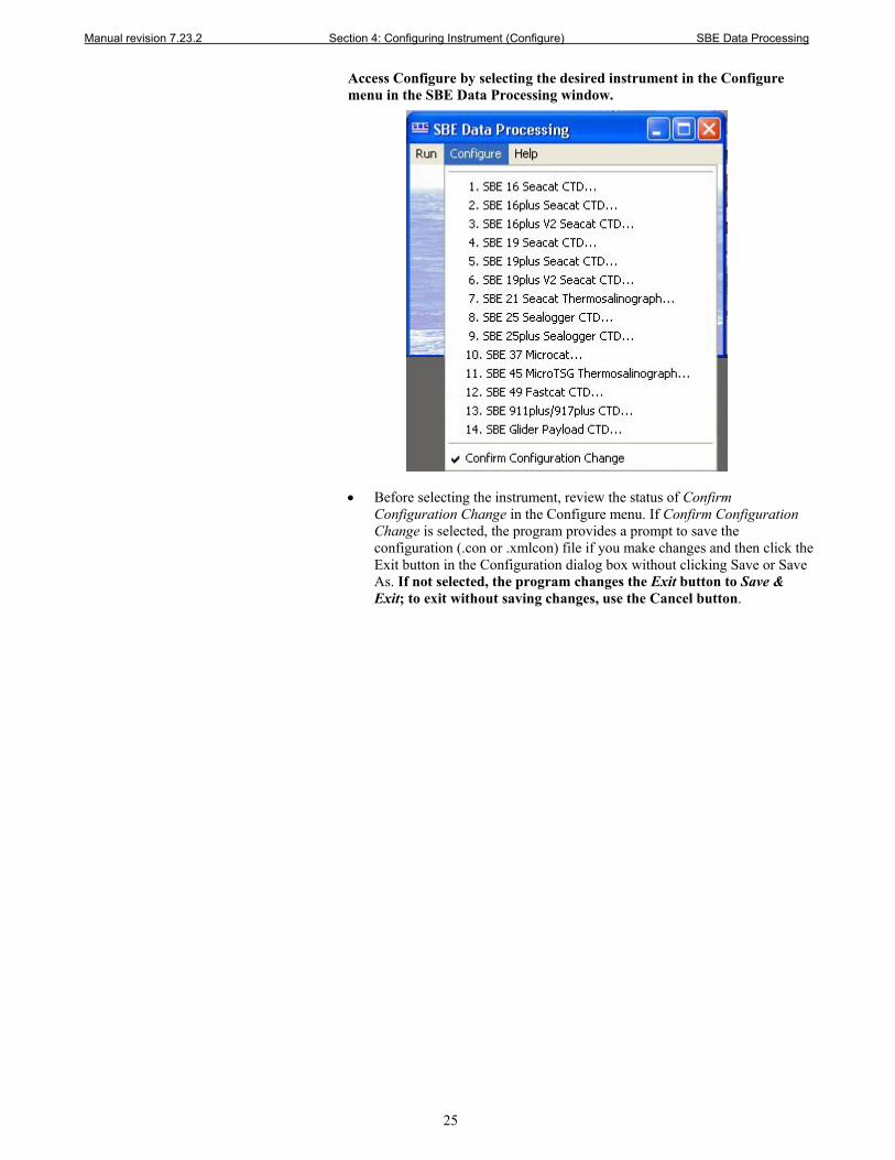
Access Configure by selecting the desired instrument in the Configure menu in the SBE Data Processing window.
• Before selecting the instrument, review the status of Confirm
Configuration Change in the Configure menu. If Confirm Configuration Change is selected, the program provides a prompt to save the configuration (.con or .xmlcon) file if you make changes and then click the Exit button in the Configuration dialog box without clicking Save or Save As. If not selected, the program changes the Exit button to Save & Exit; to exit without saving changes, use the Cancel button.
Manual revision 7.23.2 Section 4: Configuring Instrument (Configure) SBE Data Processing
26
Instrument Configuration
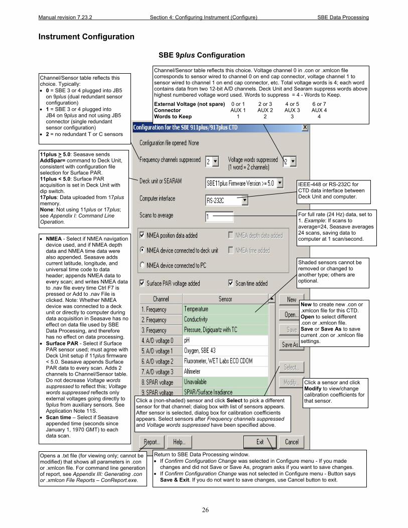
SBE 9plus Configuration
• NMEA - Select if NMEA navigation device used, and if NMEA depth data and NMEA time data were also appended. Seasave adds current latitude, longitude, and universal time code to data header; appends NMEA data to every scan; and writes NMEA data to .nav file every time Ctrl F7 is pressed or Add to .nav File is clicked. Note: Whether NMEA device was connected to a deck unit or directly to computer during data acquisition in Seasave has no effect on data file used by SBE Data Processing, and therefore has no effect on data processing.
• Surface PAR - Select if Surface PAR sensor used; must agree with Deck Unit setup if 11plus firmware < 5.0. Seasave appends Surface PAR data to every scan. Adds 2 channels to Channel/Sensor table. Do not decrease Voltage words suppressed to reflect this; Voltage words suppressed reflects only external voltages going directly to 9plus from auxiliary sensors. See Application Note 11S.
• Scan time – Select if Seasave appended time (seconds since January 1, 1970 GMT) to each data scan.
Click a sensor and click Modify to view/change calibration coefficients for that sensor.
Shaded sensors cannot be removed or changed to another type; others are optional.
IEEE-448 or RS-232C for CTD data interface between Deck Unit and computer.
Channel/Sensor table reflects this choice. Typically: • 0 = SBE 3 or 4 plugged into JB5
on 9plus (dual redundant sensor configuration)
• 1 = SBE 3 or 4 plugged into JB4 on 9plus and not using JB5 connector (single redundant sensor configuration)
• 2 = no redundant T or C sensors
Click a (non-shaded) sensor and click Select to pick a different sensor for that channel; dialog box with list of sensors appears. After sensor is selected, dialog box for calibration coefficients appears. Select sensors after Frequency channels suppressed and Voltage words suppressed have been specified above.
Channel/Sensor table reflects this choice. Voltage channel 0 in .con or .xmlcon file corresponds to sensor wired to channel 0 on end cap connector, voltage channel 1 to sensor wired to channel 1 on end cap connector, etc. Total voltage words is 4; each word contains data from two 12-bit A/D channels. Deck Unit and Searam suppress words above highest numbered voltage word used. Words to suppress = 4 - Words to Keep.
External Voltage (not spare) 0 or 1 2 or 3 4 or 5 6 or 7 Connector AUX 1 AUX 2 AUX 3 AUX 4 Words to Keep 1 2 3 4
New to create new .con or .xmlcon file for this CTD. Open to select different .con or .xmlcon file. Save or Save As to save current .con or .xmlcon file settings.
Return to SBE Data Processing window. • If Confirm Configuration Change was selected in Configure menu - If you made
changes and did not Save or Save As, program asks if you want to save changes. • If Confirm Configuration Change was not selected in Configure menu - Button says
Save & Exit. If you do not want to save changes, use Cancel button to exit.
For full rate (24 Hz) data, set to 1. Example: If scans to average=24, Seasave averages 24 scans, saving data to computer at 1 scan/second.
11plus > 5.0: Seasave sends AddSpar= command to Deck Unit, consistent with configuration file selection for Surface PAR. 11plus < 5.0: Surface PAR acquisition is set in Deck Unit with dip switch. 17plus: Data uploaded from 17plus memory. None: Not using 11plus or 17plus; see Appendix I: Command Line Operation.
Opens a .txt file (for viewing only; cannot be modified) that shows all parameters in .con or .xmlcon file. For command line generation of report, see Appendix III: Generating .con or .xmlcon File Reports – ConReport.exe.
Manual revision 7.23.2 Section 4: Configuring Instrument (Configure) SBE Data Processing
27
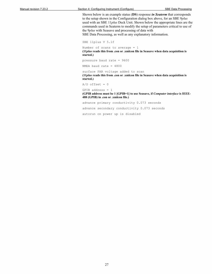
Shown below is an example status (DS) response in Seaterm that corresponds to the setup shown in the Configuration dialog box above, for an SBE 9plus used with an SBE 11plus Deck Unit. Shown below the appropriate lines are the commands used in Seaterm to modify the setup of parameters critical to use of the 9plus with Seasave and processing of data with SBE Data Processing, as well as any explanatory information. SBE 11plus V 5.1f
Number of scans to average = 1 (11plus reads this from .con or .xmlcon file in Seasave when data acquisition is started.)
pressure baud rate = 9600
NMEA baud rate = 4800
surface PAR voltage added to scan (11plus reads this from .con or .xmlcon file in Seasave when data acquisition is started.)
A/D offset = 0
GPIB address = 1 (GPIB address must be 1 [GPIB=1] to use Seasave, if Computer interface is IEEE-488 (GPIB) in .con or .xmlcon file.)
advance primary conductivity 0.073 seconds
advance secondary conductivity 0.073 seconds
autorun on power up is disabled

Manual revision 7.23.2 Section 4: Configuring Instrument (Configure) SBE Data Processing
28
SBE 16 Seacat C-T Recorder Configuration
Shown below is an example status (DS) response in Seaterm that corresponds to the setup shown in the Configuration dialog box above. Shown below the appropriate lines are the commands used in Seaterm to modify the setup of parameters critical to use of the SBE 16 with Seasave and processing of data with SBE Data Processing, as well as any explanatory information. SEACAT V4.0h SERIAL NO. 1814 07/14/95 09:52:52.082
(If pressure sensor installed, pressure sensor information appears here in status response; must match Pressure sensor type in .con or .xmlcon file.)
clk = 32767.789, iop = 103, vmain = 8.9, vlith = 5.9
sample interval = 15 sec (Sample interval [SI] must match Sample interval seconds in .con or .xmlcon file.)
delay before measuring volts = 4 seconds
samples = 0, free = 173880, lwait = 0 msec
SW1 = C2H, battery cutoff = 5.6 volts
no. of volts sampled = 2 (Number of auxiliary voltage sensors enabled [SVn] must match External voltage channels in .con or .xmlcon file.)
mode = normal
logdata = NO
Time between scans. Must agree with SBE 16 setup (SI); see reply from DS.
Select if using with deck unit connected to NMEA navigation device. Seasave adds current latitude, longitude, and universal time code to data header; appends NMEA data to every scan; and writes NMEA data to .nav file every time Ctrl F7 is pressed or Add to .nav File is clicked.
Strain gauge, Digiquartz with or without temperature compensation, or no pressure sensor. If no pressure sensor or Digiquartz without Temp Comp is selected, Data button accesses dialog box to input additional parameter(s) needed to process data.
Click a sensor and click Modify to change calibration coefficients for that sensor.
New to create new .con or .xmlcon file for this CTD. Open to select different .con or .xmlcon file. Save or Save As to save current .con or .xmlcon file settings.
Opens a .txt file (for viewing only; cannot be modified) that shows all parameters in .con or .xmlcon file. For command line generation of report, see Appendix III: Generating .con or .xmlcon File Reports – ConReport.exe.
Channel/Sensor table reflects this choice. Must agree with SBE 16 setup for SVn (n=0, 1, 2, 3, 4); see reply from DS. Voltage channel 0 in .con or .xmlcon file corresponds to sensor wired to channel 0 on end cap connector, voltage channel 1 corresponds to sensor wired to channel 1 on end cap connector, etc.
Shaded sensors cannot be removed or changed to another type of sensor. All others are optional.
Return to SBE Data Processing window. • If Confirm Configuration Change was selected in Configure menu - If you made
changes and did not Save or Save As, program asks if you want to save changes. • If Confirm Configuration Change was not selected in Configure menu - Button says
Save & Exit. If you do not want to save changes, use Cancel button to exit.
See reply from DS. Used to determine strain gauge pressure sensor data format.
Click a (non-shaded) sensor and click Select to pick a different sensor for that channel. A dialog box with a list of sensors appears. Select sensors after number of voltage channels have been specified above.
Select if Seasave appended time (seconds since January 1, 1970 GMT) to each data scan.
Manual revision 7.23.2 Section 4: Configuring Instrument (Configure) SBE Data Processing
29
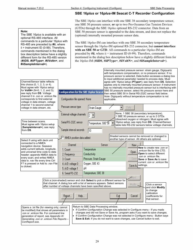
SBE 16plus or 16plus-IM Seacat C-T Recorder Configuration
The SBE 16plus can interface with one SBE 38 secondary temperature sensor, one SBE 50 pressure sensor, or up to two Pro-Oceanus Gas Tension Devices (GTDs) through the SBE 16plus optional RS-232 connector. Data from an SBE 50 pressure sensor is appended to the data stream, and does not replace the (optional) internally mounted pressure sensor data.
The SBE 16plus-IM can interface with one SBE 38 secondary temperature sensor through the 16plus-IM optional RS-232 connector, but cannot interface with an SBE 50 or GTD. All commands to a particular 16plus-IM are preceded by #ii, where ii = instrument ID (0-99). Therefore, commands mentioned in the dialog box description below have a slightly different form for the 16plus-IM (#iiDS, #iiPType=, #iiVoltN=, and #iiSampleInterval=).
Internally mounted pressure sensor: strain gauge, Digiquartz with temperature compensation, or no pressure sensor. If no pressure sensor is selected, Data button accesses a dialog box to input additional parameter needed to process data. Must agree with 16plus setup (PType=); see reply from DS. Selection applies only to internally mounted pressure sensor; if instrument has no internally mounted pressure sensor but is interfacing with SBE 50 pressure sensor, select No pressure sensor here and then select SBE 50 in Serial RS-232C sensor field below. Note: Digiquartz without temperature compensation is not applicable.
Click a sensor and click Modify to change calibration coefficients for that sensor.
New to create new .con or .xmlcon file for this CTD. Open to select different .con or .xmlcon file. Save or Save As to save current .con or .xmlcon file settings.
Channel/Sensor table reflects this choice (0, 1, 2, 3, or 4). Must agree with 16plus setup for VoltN= (N=0, 1, 2, and 3); see reply from DS. Voltage channel 0 in .con or .xmlcon file corresponds to first external voltage in data stream, voltage channel 1 to second external voltage in data stream, etc.
Shaded sensors cannot be removed or changed to another type of sensor. All others are optional.
Return to SBE Data Processing window. • If Confirm Configuration Change was selected in Configure menu - If you made
changes and did not Save or Save As, program asks if you want to save changes. • If Confirm Configuration Change was not selected in Configure menu - Button says
Save & Exit. If you do not want to save changes, use Cancel button to exit.
Select if using with deck unit connected to a NMEA navigation device. Seasave adds current latitude, longitude, and universal time code to data header; appends NMEA data to every scan; and writes NMEA data to .nav file every time Ctrl F7 is pressed or Add to .nav File is clicked.
None, 1 SBE 38 (secondary temperature), 1 SBE 50 pressure sensor, or up to 2 GTDs (dissolved oxygen or nitrogen). Must agree with 16plus setup; see reply from DS. Channel/Sensor table lists RS-232 sensors below voltage channels.
Time between scans. Must agree with 16plus setup (SampleInterval=); see reply from DS.
Click a (non-shaded) sensor and click Select to pick a different sensor for that channel. A dialog box with a list of sensors appears. Select sensors after number of voltage channels have been specified above.
Opens a .txt file (for viewing only; cannot be modified) that shows all parameters in .con or .xmlcon file. For command line generation of report, see Appendix III: Generating .con or .xmlcon File Reports – ConReport.exe.
Note: The SBE 16plus is available with an optional RS-485 interface. All commands to a particular 16plus with RS-485 are preceded by #ii, where ii = instrument ID (0-99). Therefore, commands mentioned in the dialog box description below have a slightly different form for the RS-485 version (#iiDS, #iiPType=, #iiVoltn=, and #iiSampleInterval=).
Manual revision 7.23.2 Section 4: Configuring Instrument (Configure) SBE Data Processing
30
Shown below is an example status (DS) response in Seaterm for a 16plus with standard RS-232 interface that corresponds to the setup shown in the Configuration dialog box above. Shown below the appropriate lines are the commands used in Seaterm to modify the setup of parameters critical to use of the SBE 16plus with Seasave and processing of data with SBE Data Processing, as well as any explanatory information. SBE 16plus V 1.6e SERIAL NO. 4300 03 Mar 2005 14:11:48
vbatt = 10.3, vlith = 8.5, ioper = 62.5 ma, ipump = 21.6 ma, iext01 = 76.2 ma, iserial = 48.2 ma
status = not logging
sample interval = 10 seconds, number of measurements per sample = 2 (Sample interval [SampleInterval=] must match Sample interval seconds in .con or .xmlcon file.)
samples = 823, free = 465210
run pump during sample, delay before sampling = 2.0 seconds
transmit real-time = yes (Real-time data transmission must be enabled [TxRealTime=Y] to acquire data in Seasave.)
battery cutoff = 7.5 volts
pressure sensor = strain gauge, range = 1000.0 (Internal pressure sensor [PType=] must match Pressure sensor type in .con or .xmlcon file.)
SBE 38 = yes, SBE 50 = no, Gas Tension Device = no (Selection/enabling of RS-232 sensors [SBE38=, SBE50=, GTD=, DualGTD=] must match Serial RS-232C sensor in .con or .xmlcon file.)
Ext Volt 0 = yes, Ext Volt 1 = yes, Ext Volt 2 = no, Ext Volt 3 = no (Number of external voltage sensors enabled [Volt0= through Volt3=] must match External voltage channels in .con or .xmlcon file.)
echo commands = yes
output format = raw HEX (Output format must be set to raw Hex [OutputFormat=0] to acquire data in Seasave.)
serial sync mode disabled (Serial sync mode must be disabled [SyncMode=N] to acquire data in Seasave.)
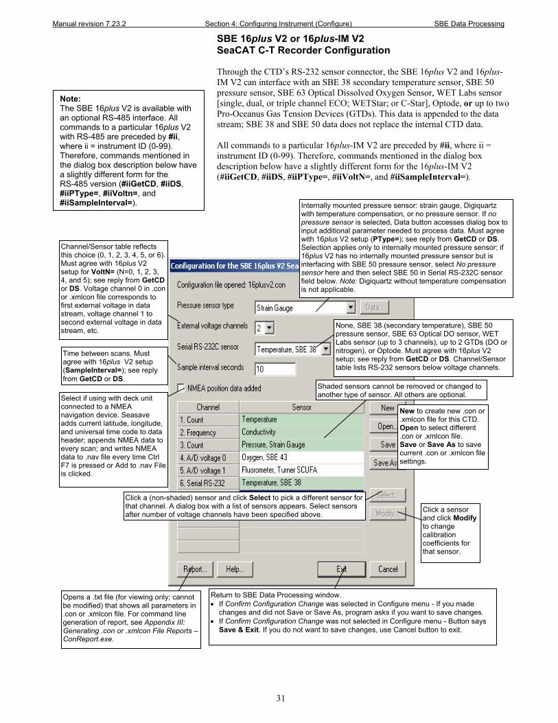
Manual revision 7.23.2 Section 4: Configuring Instrument (Configure) SBE Data Processing
31
SBE 16plus V2 or 16plus-IM V2 SeaCAT C-T Recorder Configuration
Through the CTD’s RS-232 sensor connector, the SBE 16plus V2 and 16plus-IM V2 can interface with an SBE 38 secondary temperature sensor, SBE 50 pressure sensor, SBE 63 Optical Dissolved Oxygen Sensor, WET Labs sensor [single, dual, or triple channel ECO; WETStar; or C-Star], Optode, or up to two Pro-Oceanus Gas Tension Devices (GTDs). This data is appended to the data stream; SBE 38 and SBE 50 data does not replace the internal CTD data.
All commands to a particular 16plus-IM V2 are preceded by #ii, where ii = instrument ID (0-99). Therefore, commands mentioned in the dialog box description below have a slightly different form for the 16plus-IM V2 (#iiGetCD, #iiDS, #iiPType=, #iiVoltN=, and #iiSampleInterval=).
Note: The SBE 16plus V2 is available with an optional RS-485 interface. All commands to a particular 16plus V2 with RS-485 are preceded by #ii, where ii = instrument ID (0-99). Therefore, commands mentioned in the dialog box description below have a slightly different form for the RS-485 version (#iiGetCD, #iiDS, #iiPType=, #iiVoltn=, and #iiSampleInterval=). Internally mounted pressure sensor: strain gauge, Digiquartz
with temperature compensation, or no pressure sensor. If no pressure sensor is selected, Data button accesses dialog box to input additional parameter needed to process data. Must agree with 16plus V2 setup (PType=); see reply from GetCD or DS. Selection applies only to internally mounted pressure sensor; if 16plus V2 has no internally mounted pressure sensor but is interfacing with SBE 50 pressure sensor, select No pressure sensor here and then select SBE 50 in Serial RS-232C sensor field below. Note: Digiquartz without temperature compensation is not applicable.
Click a sensor and click Modify to change calibration coefficients for that sensor.
New to create new .con or .xmlcon file for this CTD. Open to select different .con or .xmlcon file. Save or Save As to save current .con or .xmlcon file settings.
Channel/Sensor table reflects this choice (0, 1, 2, 3, 4, 5, or 6). Must agree with 16plus V2 setup for VoltN= (N=0, 1, 2, 3, 4, and 5); see reply from GetCD or DS. Voltage channel 0 in .con or .xmlcon file corresponds to first external voltage in data stream, voltage channel 1 to second external voltage in data stream, etc.
Shaded sensors cannot be removed or changed to another type of sensor. All others are optional.
Return to SBE Data Processing window. • If Confirm Configuration Change was selected in Configure menu - If you made
changes and did not Save or Save As, program asks if you want to save changes. • If Confirm Configuration Change was not selected in Configure menu - Button says
Save & Exit. If you do not want to save changes, use Cancel button to exit.
Select if using with deck unit connected to a NMEA navigation device. Seasave adds current latitude, longitude, and universal time code to data header; appends NMEA data to every scan; and writes NMEA data to .nav file every time Ctrl F7 is pressed or Add to .nav File is clicked.
None, SBE 38 (secondary temperature), SBE 50 pressure sensor, SBE 63 Optical DO sensor, WET Labs sensor (up to 3 channels), up to 2 GTDs (DO or nitrogen), or Optode. Must agree with 16plus V2 setup; see reply from GetCD or DS. Channel/Sensor table lists RS-232 sensors below voltage channels.
Time between scans. Must agree with 16plus V2 setup (SampleInterval=); see reply from GetCD or DS.
Click a (non-shaded) sensor and click Select to pick a different sensor for that channel. A dialog box with a list of sensors appears. Select sensors after number of voltage channels have been specified above.
Opens a .txt file (for viewing only; cannot be modified) that shows all parameters in .con or .xmlcon file. For command line generation of report, see Appendix III: Generating .con or .xmlcon File Reports – ConReport.exe.
Manual revision 7.23.2 Section 4: Configuring Instrument (Configure) SBE Data Processing
32
Shown below is an example status (DS) response in a terminal program for a 16plus V2 with standard RS-232 interface that corresponds to the setup shown in the Configuration dialog box above. Shown below the appropriate lines are the commands used in the terminal program to modify the setup of parameters critical to use of the SBE 16plus V2 with Seasave and processing of data with SBE Data Processing, as well as any explanatory information.
SBE 16plus V 2.0 SERIAL NO. 6001 24 Oct 2007 14:11:48
vbatt = 10.3, vlith = 8.5, ioper = 62.5 ma, ipump = 21.6 ma, iext01 = 76.2 ma, iserial = 48.2 ma
status = not logging
samples = 0, free = 3463060
sample interval = 10 seconds, number of measurements per sample = 1 (Sample interval [SampleInterval=] must match Sample interval seconds in .con or .xmlcon file.)
pump = run pump during sample, delay before sampling = 2.0 seconds
transmit real-time = yes (Real-time data transmission must be enabled [TxRealTime=Y] to acquire data in Seasave.)
battery cutoff = 7.5 volts
pressure sensor = strain gauge, range = 1000.0 (Internal pressure sensor [PType=] must match Pressure sensor type in .con or .xmlcon file.)
SBE 38 = yes, SBE 50 = no, WETLABS = no, OPTODE = no, SBE63 = no, Gas Tension Device = no (Selection/enabling of RS-232 sensors [SBE38=, SBE50=, WetLabs=, Optode=, SBE63=, GTD=, DualGTD=] must match Serial RS-232C sensor in .con or .xmlcon file.)
Ext Volt 0 = yes, Ext Volt 1 = yes, Ext Volt 2 = no, Ext Volt 3 = no, Ext Volt4 = no, Ext Volt 5 = no (Number of external voltage sensors enabled [Volt0= through Volt5=] must match External voltage channels in .con or .xmlcon file.)
echo characters = yes
output format = raw HEX (Output format must be set to raw Hex [OutputFormat=0] to acquire data in Seasave.)
serial sync mode disabled (Serial sync mode must be disabled [SyncMode=N] to acquire data in Seasave.)
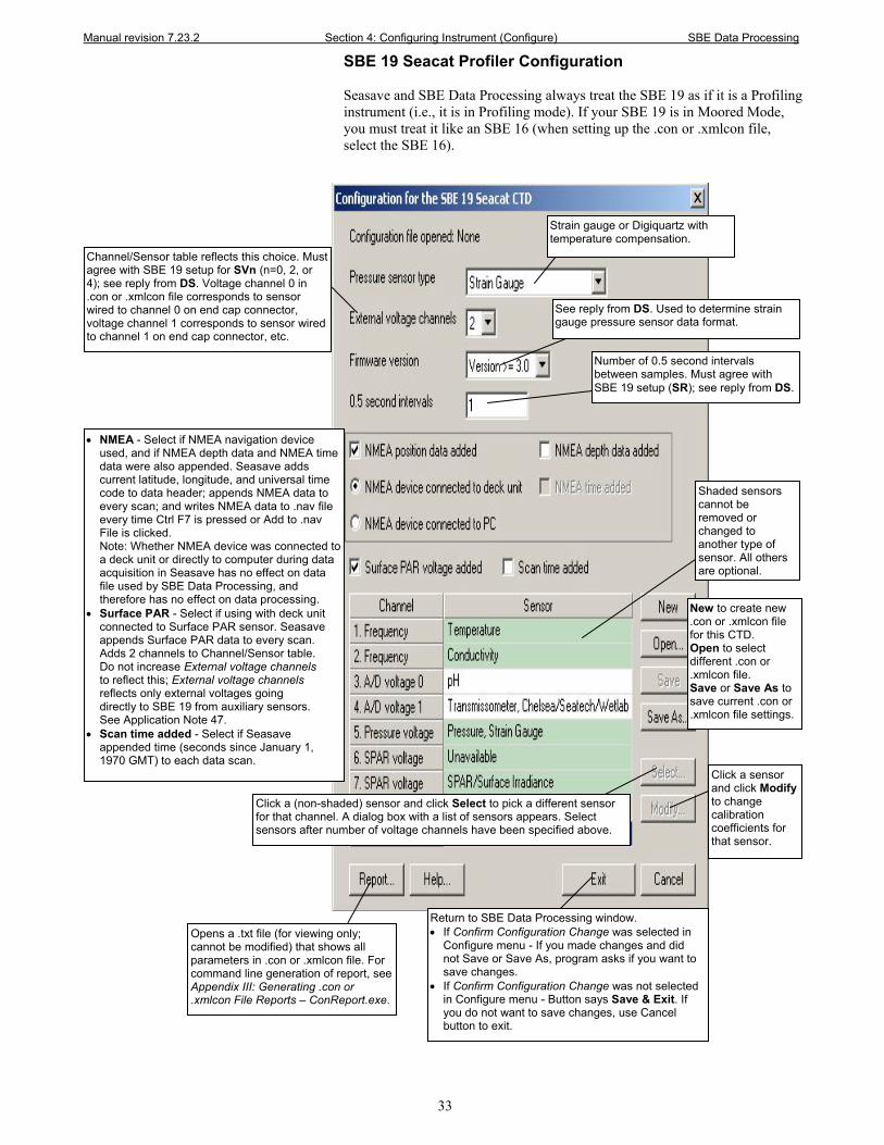
Manual revision 7.23.2 Section 4: Configuring Instrument (Configure) SBE Data Processing
33
SBE 19 Seacat Profiler Configuration
Seasave and SBE Data Processing always treat the SBE 19 as if it is a Profiling instrument (i.e., it is in Profiling mode). If your SBE 19 is in Moored Mode, you must treat it like an SBE 16 (when setting up the .con or .xmlcon file, select the SBE 16).
See reply from DS. Used to determine strain gauge pressure sensor data format.
Number of 0.5 second intervals between samples. Must agree with SBE 19 setup (SR); see reply from DS.
• NMEA - Select if NMEA navigation device used, and if NMEA depth data and NMEA time data were also appended. Seasave adds current latitude, longitude, and universal time code to data header; appends NMEA data to every scan; and writes NMEA data to .nav file every time Ctrl F7 is pressed or Add to .nav File is clicked. Note: Whether NMEA device was connected to a deck unit or directly to computer during data acquisition in Seasave has no effect on data file used by SBE Data Processing, and therefore has no effect on data processing.
• Surface PAR - Select if using with deck unit connected to Surface PAR sensor. Seasave appends Surface PAR data to every scan. Adds 2 channels to Channel/Sensor table. Do not increase External voltage channels to reflect this; External voltage channels reflects only external voltages going directly to SBE 19 from auxiliary sensors. See Application Note 47.
• Scan time added - Select if Seasave appended time (seconds since January 1, 1970 GMT) to each data scan.
Strain gauge or Digiquartz with temperature compensation.
Click a sensor and click Modify to change calibration coefficients for that sensor.
New to create new .con or .xmlcon file for this CTD. Open to select different .con or .xmlcon file. Save or Save As to save current .con or .xmlcon file settings.
Shaded sensors cannot be removed or changed to another type of sensor. All others are optional.
Return to SBE Data Processing window. • If Confirm Configuration Change was selected in
Configure menu - If you made changes and did not Save or Save As, program asks if you want to save changes.
• If Confirm Configuration Change was not selected in Configure menu - Button says Save & Exit. If you do not want to save changes, use Cancel button to exit.
Opens a .txt file (for viewing only; cannot be modified) that shows all parameters in .con or .xmlcon file. For command line generation of report, see Appendix III: Generating .con or .xmlcon File Reports – ConReport.exe.
Click a (non-shaded) sensor and click Select to pick a different sensor for that channel. A dialog box with a list of sensors appears. Select sensors after number of voltage channels have been specified above.
Channel/Sensor table reflects this choice. Must agree with SBE 19 setup for SVn (n=0, 2, or 4); see reply from DS. Voltage channel 0 in .con or .xmlcon file corresponds to sensor wired to channel 0 on end cap connector, voltage channel 1 corresponds to sensor wired to channel 1 on end cap connector, etc.
Manual revision 7.23.2 Section 4: Configuring Instrument (Configure) SBE Data Processing
34
Shown below is an example status (DS) response in Seaterm that corresponds to the setup shown in the Configuration dialog box above. Shown below the appropriate lines are the commands used in Seaterm to modify the setup of parameters critical to use of the SBE 19 with Seasave and processing of data with SBE Data Processing, as well as any explanatory information. SEACAT PROFILER V3.1B SN 936 02/10/94 13:33:23.989
strain gauge pressure sensor: S/N = 12345, range = 1000 psia, tc = 240 (Pressure sensor (strain gauge or Digiquartz) must match Pressure sensor type in .con or .xmlcon file.)
clk = 32767.766 iop = 172 vmain = 8.1 vlith = 5.8
mode = PROFILE ncasts = 0 (Mode must be profile [MP] if setting up .con or .xmlcon file for SBE 19; create .con or .xmlcon file for SBE 16 for SBE 19 in moored mode [MM].)
sample rate = 1 scan every 0.5 seconds (Sample rate [SR] must match 0.5 second intervals in .con or .xmlcon file.)
minimum raw conductivity frequency for pump turn on = 3206 hertz
pump delay = 40 seconds
samples = 0 free = 174126 lwait = 0 msec
battery cutoff = 7.2 volts
number of voltages sampled = 2 (Number of auxiliary voltage sensors enabled [SVn] must match External voltage channels in .con or .xmlcon file.)
logdata = NO
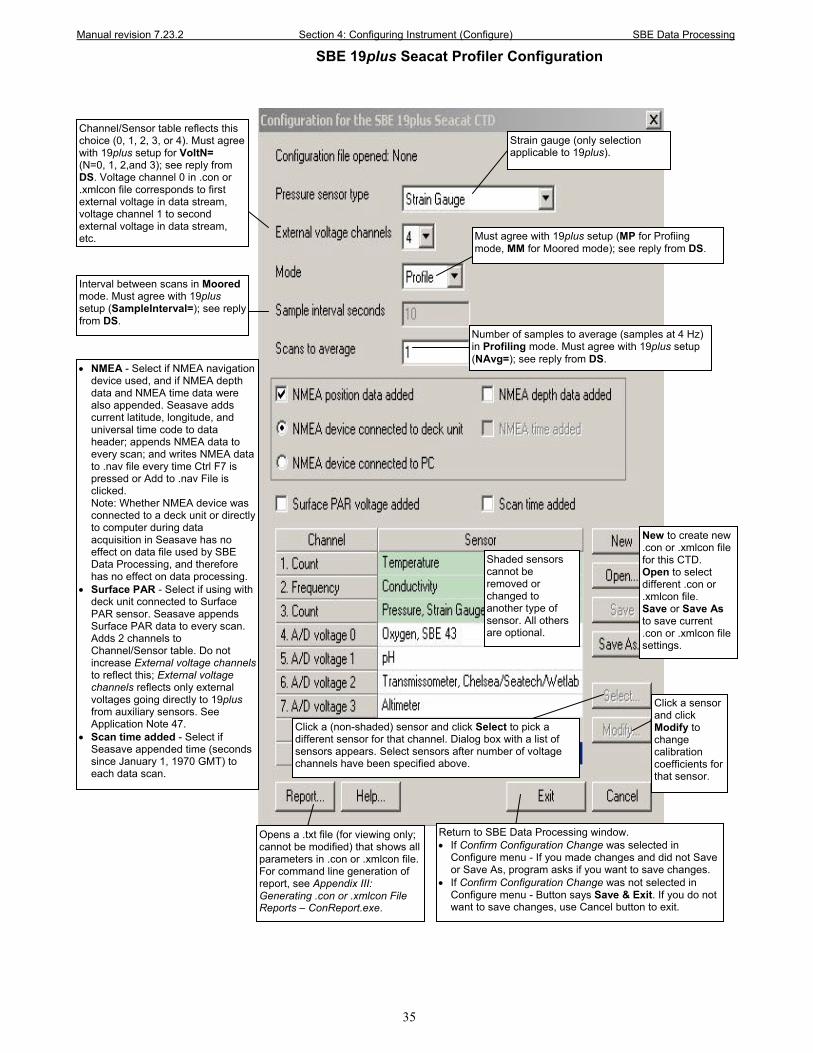
Manual revision 7.23.2 Section 4: Configuring Instrument (Configure) SBE Data Processing
35
SBE 19plus Seacat Profiler Configuration
Must agree with 19plus setup (MP for Profiing mode, MM for Moored mode); see reply from DS.
• NMEA - Select if NMEA navigation device used, and if NMEA depth data and NMEA time data were also appended. Seasave adds current latitude, longitude, and universal time code to data header; appends NMEA data to every scan; and writes NMEA data to .nav file every time Ctrl F7 is pressed or Add to .nav File is clicked. Note: Whether NMEA device was connected to a deck unit or directly to computer during data acquisition in Seasave has no effect on data file used by SBE Data Processing, and therefore has no effect on data processing.
• Surface PAR - Select if using with deck unit connected to Surface PAR sensor. Seasave appends Surface PAR data to every scan. Adds 2 channels to Channel/Sensor table. Do not increase External voltage channels to reflect this; External voltage channels reflects only external voltages going directly to 19plus from auxiliary sensors. See Application Note 47.
• Scan time added - Select if Seasave appended time (seconds since January 1, 1970 GMT) to each data scan.
Strain gauge (only selection applicable to 19plus).
Click a (non-shaded) sensor and click Select to pick a different sensor for that channel. Dialog box with a list of sensors appears. Select sensors after number of voltage channels have been specified above.
Click a sensor and click Modify to change calibration coefficients for that sensor.
New to create new .con or .xmlcon file for this CTD. Open to select different .con or .xmlcon file. Save or Save As to save current .con or .xmlcon file settings.
Channel/Sensor table reflects this choice (0, 1, 2, 3, or 4). Must agree with 19plus setup for VoltN= (N=0, 1, 2,and 3); see reply from DS. Voltage channel 0 in .con or .xmlcon file corresponds to first external voltage in data stream, voltage channel 1 to second external voltage in data stream, etc.
Shaded sensors cannot be removed or changed to another type of sensor. All others are optional.
Return to SBE Data Processing window. • If Confirm Configuration Change was selected in
Configure menu - If you made changes and did not Save or Save As, program asks if you want to save changes.
• If Confirm Configuration Change was not selected in Configure menu - Button says Save & Exit. If you do not want to save changes, use Cancel button to exit.
Interval between scans in Moored mode. Must agree with 19plus setup (SampleInterval=); see reply from DS.
Number of samples to average (samples at 4 Hz) in Profiling mode. Must agree with 19plus setup (NAvg=); see reply from DS.
Opens a .txt file (for viewing only; cannot be modified) that shows all parameters in .con or .xmlcon file. For command line generation of report, see Appendix III: Generating .con or .xmlcon File Reports – ConReport.exe.

Manual revision 7.23.2 Section 4: Configuring Instrument (Configure) SBE Data Processing
36
Shown below is an example status (DS) response in Seaterm that corresponds to the setup shown in the Configuration dialog box above. Shown below the appropriate lines are the commands used in Seaterm to modify the setup of parameters critical to use of the 19plus with Seasave and processing of data with SBE Data Processing, as well as any explanatory information. SeacatPlus V 1.5 SERIAL NO. 4000 22 May 2005 14:02:13
vbatt = 9.6, vlith = 8.6, ioper = 61.2 ma, ipump = 25.5 ma, iext01 = 76.2 ma, iext23 = 65.1 ma
status = not logging
number of scans to average = 1 (Scans to average [NAvg=] must match Scans to Average in .con or .xmlcon file.)
samples = 0, free = 381300, casts = 0
mode = profile, minimum cond freq = 3000, pump delay = 60 sec (Mode [MP for profile or MM for moored] must match Mode in .con or .xmlcon file.)
autorun = no, ignore magnetic switch = no
battery type = ALKALINE, battery cutoff = 7.3 volts
pressure sensor = strain gauge, range = 1000.0 (Pressure sensor [PType=] must match Pressure sensor type in .con or .xmlcon file.)
SBE 38 = no, Gas Tension Device = no (RS-232 sensors (which are used for custom applications only) must be disabled to use Seasave.)
Ext Volt 0 = yes, Ext Volt 1 = yes, Ext Volt 2 = yes, Ext Volt 3 = yes (Number of external voltage sensors enabled [Volt0= through Volt3=] must match External voltage channels in .con or .xmlcon file.)
echo commands = yes
output format = raw Hex (Output format must be set to raw Hex [OutputFormat=0] to acquire data in Seasave.)
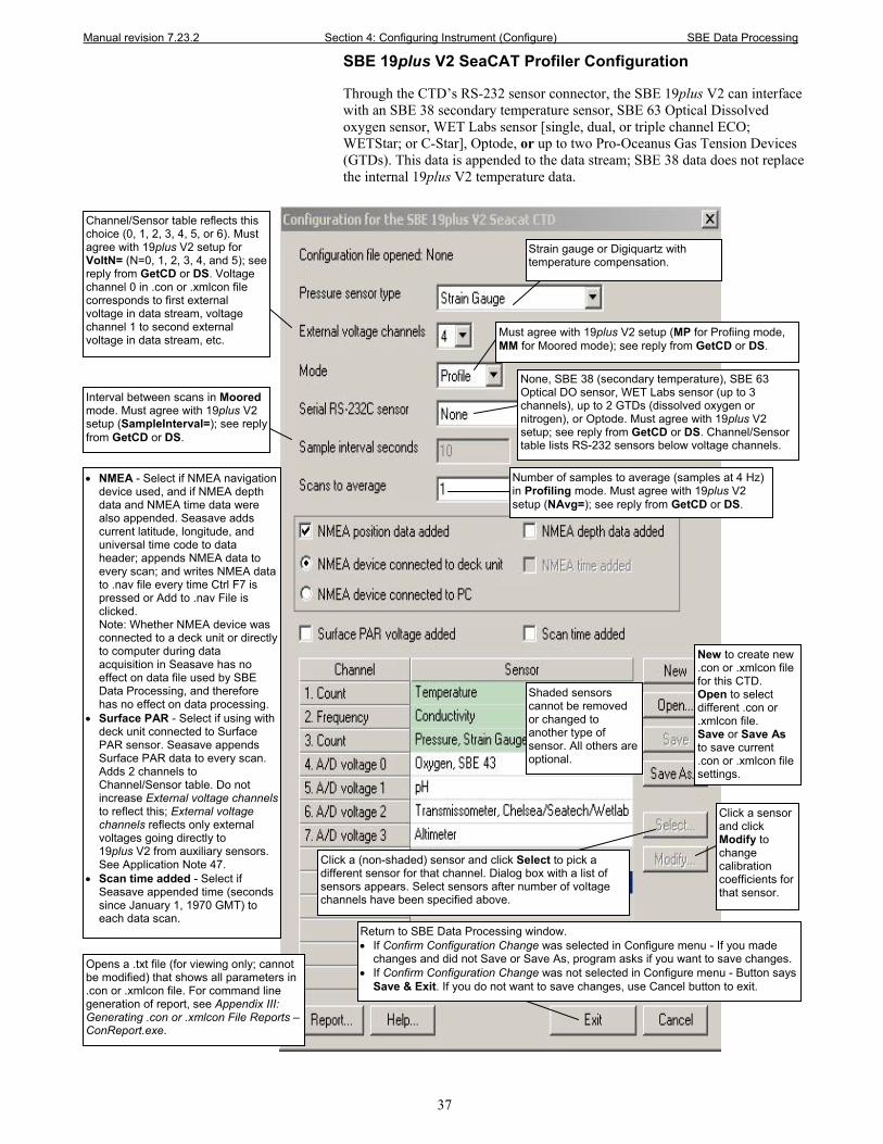
Manual revision 7.23.2 Section 4: Configuring Instrument (Configure) SBE Data Processing
37
SBE 19plus V2 SeaCAT Profiler Configuration
Through the CTD’s RS-232 sensor connector, the SBE 19plus V2 can interface with an SBE 38 secondary temperature sensor, SBE 63 Optical Dissolved oxygen sensor, WET Labs sensor [single, dual, or triple channel ECO; WETStar; or C-Star], Optode, or up to two Pro-Oceanus Gas Tension Devices (GTDs). This data is appended to the data stream; SBE 38 data does not replace the internal 19plus V2 temperature data.
Must agree with 19plus V2 setup (MP for Profiing mode, MM for Moored mode); see reply from GetCD or DS.
• NMEA - Select if NMEA navigation device used, and if NMEA depth data and NMEA time data were also appended. Seasave adds current latitude, longitude, and universal time code to data header; appends NMEA data to every scan; and writes NMEA data to .nav file every time Ctrl F7 is pressed or Add to .nav File is clicked. Note: Whether NMEA device was connected to a deck unit or directly to computer during data acquisition in Seasave has no effect on data file used by SBE Data Processing, and therefore has no effect on data processing.
• Surface PAR - Select if using with deck unit connected to Surface PAR sensor. Seasave appends Surface PAR data to every scan. Adds 2 channels to Channel/Sensor table. Do not increase External voltage channels to reflect this; External voltage channels reflects only external voltages going directly to 19plus V2 from auxiliary sensors. See Application Note 47.
• Scan time added - Select if Seasave appended time (seconds since January 1, 1970 GMT) to each data scan.
Strain gauge or Digiquartz with temperature compensation.
Click a (non-shaded) sensor and click Select to pick a different sensor for that channel. Dialog box with a list of sensors appears. Select sensors after number of voltage channels have been specified above.
Click a sensor and click Modify to change calibration coefficients for that sensor.
New to create new .con or .xmlcon file for this CTD. Open to select different .con or .xmlcon file. Save or Save As to save current .con or .xmlcon file settings.
Channel/Sensor table reflects this choice (0, 1, 2, 3, 4, 5, or 6). Must agree with 19plus V2 setup for VoltN= (N=0, 1, 2, 3, 4, and 5); see reply from GetCD or DS. Voltage channel 0 in .con or .xmlcon file corresponds to first external voltage in data stream, voltage channel 1 to second external voltage in data stream, etc.
Shaded sensors cannot be removed or changed to another type of sensor. All others are optional.
Return to SBE Data Processing window. • If Confirm Configuration Change was selected in Configure menu - If you made
changes and did not Save or Save As, program asks if you want to save changes. • If Confirm Configuration Change was not selected in Configure menu - Button says
Save & Exit. If you do not want to save changes, use Cancel button to exit.
Interval between scans in Moored mode. Must agree with 19plus V2 setup (SampleInterval=); see reply from GetCD or DS.
Number of samples to average (samples at 4 Hz) in Profiling mode. Must agree with 19plus V2 setup (NAvg=); see reply from GetCD or DS.
None, SBE 38 (secondary temperature), SBE 63 Optical DO sensor, WET Labs sensor (up to 3 channels), up to 2 GTDs (dissolved oxygen or nitrogen), or Optode. Must agree with 19plus V2 setup; see reply from GetCD or DS. Channel/Sensor table lists RS-232 sensors below voltage channels.
Opens a .txt file (for viewing only; cannot be modified) that shows all parameters in .con or .xmlcon file. For command line generation of report, see Appendix III: Generating .con or .xmlcon File Reports – ConReport.exe.
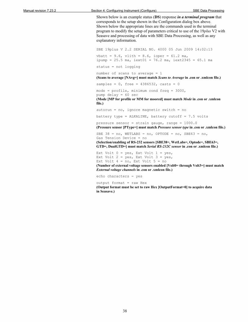
Manual revision 7.23.2 Section 4: Configuring Instrument (Configure) SBE Data Processing
38
Shown below is an example status (DS) response in a terminal program that corresponds to the setup shown in the Configuration dialog box above. Shown below the appropriate lines are the commands used in the terminal program to modify the setup of parameters critical to use of the 19plus V2 with Seasave and processing of data with SBE Data Processing, as well as any explanatory information. SBE 19plus V 2.2 SERIAL NO. 4000 05 Jun 2009 14:02:13
vbatt = 9.6, vlith = 8.6, ioper = 61.2 ma, ipump = 25.5 ma, iext01 = 76.2 ma, iext2345 = 65.1 ma
status = not logging
number of scans to average = 1 (Scans to average [NAvg=] must match Scans to Average in .con or .xmlcon file.)
samples = 0, free = 4386532, casts = 0
mode = profile, minimum cond freq = 3000, pump delay = 60 sec (Mode [MP for profile or MM for moored] must match Mode in .con or .xmlcon file.)
autorun = no, ignore magnetic switch = no
battery type = ALKALINE, battery cutoff = 7.5 volts
pressure sensor = strain gauge, range = 1000.0 (Pressure sensor [PType=] must match Pressure sensor type in .con or .xmlcon file.)
SBE 38 = no, WETLABS = no, OPTODE = no, SBE63 = no, Gas Tension Device = no (Selection/enabling of RS-232 sensors [SBE38=, WetLabs=, Optode=, SBE63=, GTD=, DualGTD=] must match Serial RS-232C sensor in .con or .xmlcon file.)
Ext Volt 0 = yes, Ext Volt 1 = yes, Ext Volt 2 = yes, Ext Volt 3 = yes, Ext Volt 4 = no, Ext Volt 5 = no (Number of external voltage sensors enabled [Volt0= through Volt3=] must match External voltage channels in .con or .xmlcon file.)
echo characters = yes
output format = raw Hex (Output format must be set to raw Hex [OutputFormat=0] to acquire data in Seasave.)
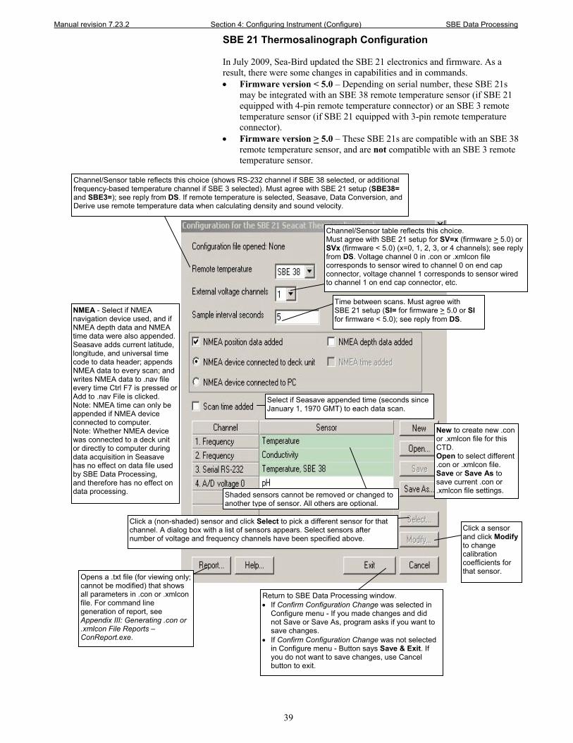
Manual revision 7.23.2 Section 4: Configuring Instrument (Configure) SBE Data Processing
39
SBE 21 Thermosalinograph Configuration
In July 2009, Sea-Bird updated the SBE 21 electronics and firmware. As a result, there were some changes in capabilities and in commands. • Firmware version < 5.0 – Depending on serial number, these SBE 21s
may be integrated with an SBE 38 remote temperature sensor (if SBE 21 equipped with 4-pin remote temperature connector) or an SBE 3 remote temperature sensor (if SBE 21 equipped with 3-pin remote temperature connector).
• Firmware version > 5.0 – These SBE 21s are compatible with an SBE 38 remote temperature sensor, and are not compatible with an SBE 3 remote temperature sensor.
Channel/Sensor table reflects this choice. Must agree with SBE 21 setup for SV=x (firmware > 5.0) or SVx (firmware < 5.0) (x=0, 1, 2, 3, or 4 channels); see reply from DS. Voltage channel 0 in .con or .xmlcon file corresponds to sensor wired to channel 0 on end cap connector, voltage channel 1 corresponds to sensor wired to channel 1 on end cap connector, etc.
NMEA - Select if NMEA navigation device used, and if NMEA depth data and NMEA time data were also appended. Seasave adds current latitude, longitude, and universal time code to data header; appends NMEA data to every scan; and writes NMEA data to .nav file every time Ctrl F7 is pressed or Add to .nav File is clicked. Note: NMEA time can only be appended if NMEA device connected to computer. Note: Whether NMEA device was connected to a deck unit or directly to computer during data acquisition in Seasave has no effect on data file used by SBE Data Processing, and therefore has no effect on data processing.
Click a sensor and click Modify to change calibration coefficients for that sensor.
New to create new .con or .xmlcon file for this CTD. Open to select different .con or .xmlcon file. Save or Save As to save current .con or .xmlcon file settings.
Opens a .txt file (for viewing only; cannot be modified) that shows all parameters in .con or .xmlcon file. For command line generation of report, see Appendix III: Generating .con or .xmlcon File Reports – ConReport.exe.
Channel/Sensor table reflects this choice (shows RS-232 channel if SBE 38 selected, or additional frequency-based temperature channel if SBE 3 selected). Must agree with SBE 21 setup (SBE38= and SBE3=); see reply from DS. If remote temperature is selected, Seasave, Data Conversion, and Derive use remote temperature data when calculating density and sound velocity.
Shaded sensors cannot be removed or changed to another type of sensor. All others are optional.
Return to SBE Data Processing window. • If Confirm Configuration Change was selected in
Configure menu - If you made changes and did not Save or Save As, program asks if you want to save changes.
• If Confirm Configuration Change was not selected in Configure menu - Button says Save & Exit. If you do not want to save changes, use Cancel button to exit.
Click a (non-shaded) sensor and click Select to pick a different sensor for that channel. A dialog box with a list of sensors appears. Select sensors after number of voltage and frequency channels have been specified above.
Time between scans. Must agree with SBE 21 setup (SI= for firmware > 5.0 or SI for firmware < 5.0); see reply from DS.
Select if Seasave appended time (seconds since January 1, 1970 GMT) to each data scan.
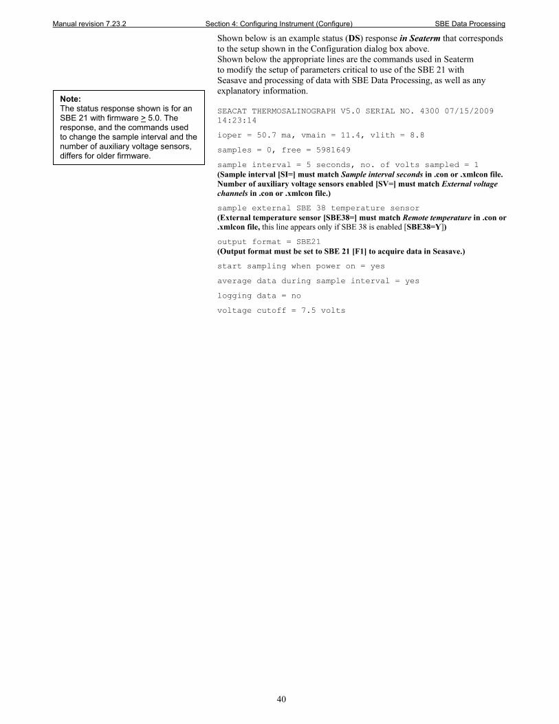
Manual revision 7.23.2 Section 4: Configuring Instrument (Configure) SBE Data Processing
40
Shown below is an example status (DS) response in Seaterm that corresponds to the setup shown in the Configuration dialog box above. Shown below the appropriate lines are the commands used in Seaterm to modify the setup of parameters critical to use of the SBE 21 with Seasave and processing of data with SBE Data Processing, as well as any explanatory information. SEACAT THERMOSALINOGRAPH V5.0 SERIAL NO. 4300 07/15/2009 14:23:14
ioper = 50.7 ma, vmain = 11.4, vlith = 8.8
samples = 0, free = 5981649
sample interval = 5 seconds, no. of volts sampled = 1 (Sample interval [SI=] must match Sample interval seconds in .con or .xmlcon file. Number of auxiliary voltage sensors enabled [SV=] must match External voltage channels in .con or .xmlcon file.)
sample external SBE 38 temperature sensor (External temperature sensor [SBE38=] must match Remote temperature in .con or .xmlcon file, this line appears only if SBE 38 is enabled [SBE38=Y])
output format = SBE21 (Output format must be set to SBE 21 [F1] to acquire data in Seasave.)
start sampling when power on = yes
average data during sample interval = yes
logging data = no
voltage cutoff = 7.5 volts
Note: The status response shown is for an SBE 21 with firmware > 5.0. The response, and the commands used to change the sample interval and the number of auxiliary voltage sensors, differs for older firmware.
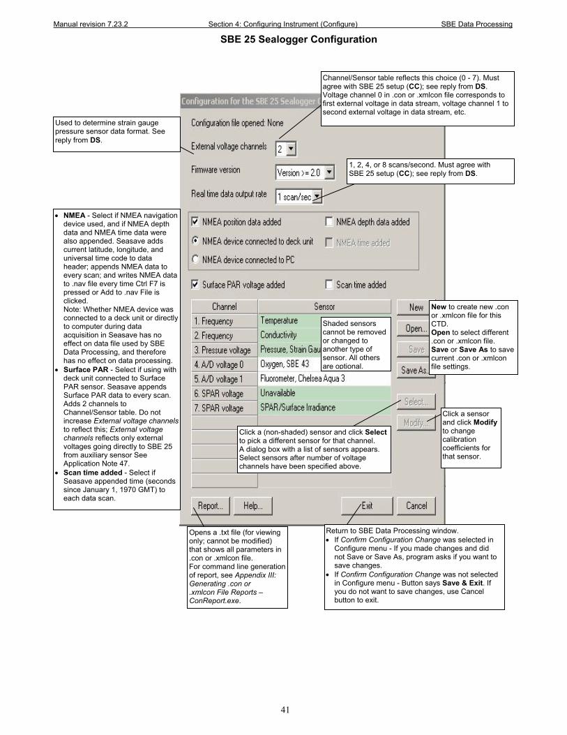
Manual revision 7.23.2 Section 4: Configuring Instrument (Configure) SBE Data Processing
41
SBE 25 Sealogger Configuration
Channel/Sensor table reflects this choice (0 - 7). Must agree with SBE 25 setup (CC); see reply from DS. Voltage channel 0 in .con or .xmlcon file corresponds to first external voltage in data stream, voltage channel 1 to second external voltage in data stream, etc.
Used to determine strain gauge pressure sensor data format. See reply from DS.
• NMEA - Select if NMEA navigation device used, and if NMEA depth data and NMEA time data were also appended. Seasave adds current latitude, longitude, and universal time code to data header; appends NMEA data to every scan; and writes NMEA data to .nav file every time Ctrl F7 is pressed or Add to .nav File is clicked. Note: Whether NMEA device was connected to a deck unit or directly to computer during data acquisition in Seasave has no effect on data file used by SBE Data Processing, and therefore has no effect on data processing.
• Surface PAR - Select if using with deck unit connected to Surface PAR sensor. Seasave appends Surface PAR data to every scan. Adds 2 channels to Channel/Sensor table. Do not increase External voltage channels to reflect this; External voltage channels reflects only external voltages going directly to SBE 25 from auxiliary sensor See Application Note 47.
• Scan time added - Select if Seasave appended time (seconds since January 1, 1970 GMT) to each data scan.
Click a sensor and click Modify to change calibration coefficients for that sensor.
New to create new .con or .xmlcon file for this CTD. Open to select different .con or .xmlcon file. Save or Save As to save current .con or .xmlcon file settings.
Shaded sensors cannot be removed or changed to another type of sensor. All others are optional.
Return to SBE Data Processing window. • If Confirm Configuration Change was selected in
Configure menu - If you made changes and did not Save or Save As, program asks if you want to save changes.
• If Confirm Configuration Change was not selected in Configure menu - Button says Save & Exit. If you do not want to save changes, use Cancel button to exit.
Opens a .txt file (for viewing only; cannot be modified) that shows all parameters in .con or .xmlcon file. For command line generation of report, see Appendix III: Generating .con or .xmlcon File Reports – ConReport.exe.
Click a (non-shaded) sensor and click Select to pick a different sensor for that channel. A dialog box with a list of sensors appears. Select sensors after number of voltage channels have been specified above.
1, 2, 4, or 8 scans/second. Must agree with SBE 25 setup (CC); see reply from DS.

Manual revision 7.23.2 Section 4: Configuring Instrument (Configure) SBE Data Processing
42
Shown below is an example status (DS) response in Seaterm that corresponds to the setup shown in the Configuration dialog box above. Shown below the appropriate lines are the commands used in Seaterm to modify the setup of parameters critical to use of the SBE 25 with Seasave and processing of data with SBE Data Processing, as well as any explanatory information. SBE 25 CTD V 4.1a SN 323 04/26/02 14:02:13
external pressure sensor, range = 5076 psia, tcval = -55
xtal=9437363 clk=32767.107 vmain=10.1 iop=175 vlith=5.6
ncasts=0 samples=0 free = 54980 lwait = 0 msec
stop upcast when CTD ascends 30 % of full scale pressure sensor range (2301 counts)
CTD configuration:
number of scans averaged=1, data stored at 8 scans per second
real time data transmitted at 1 scans per second (real-time data transmission [CC] must match Real time data output rate in .con or .xmlcon file.)
minimum conductivity frequency for pump turn on = 2950
pump delay = 45 seconds
battery type = ALKALINE
2 external voltages sampled (Number of auxiliary voltage sensors enabled [CC] must match External voltage channels in .con or .xmlcon file.)
stored voltage #0 = external voltage 0
stored voltage #1 = external voltage 1
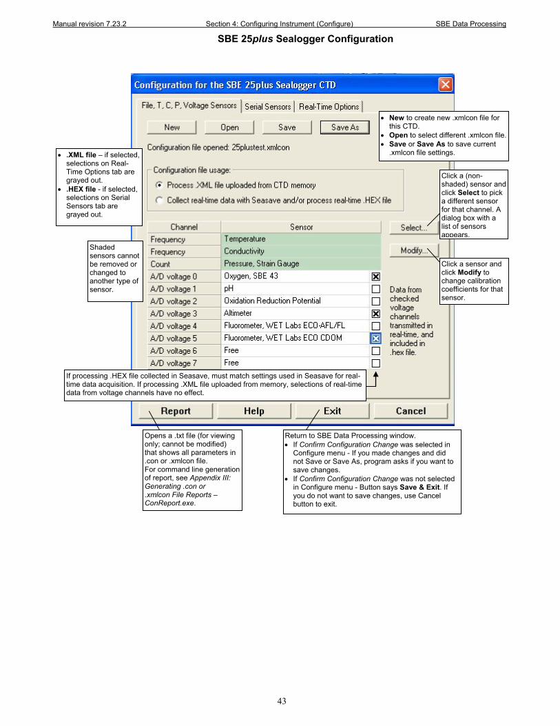
Manual revision 7.23.2 Section 4: Configuring Instrument (Configure) SBE Data Processing
43
SBE 25plus Sealogger Configuration
Return to SBE Data Processing window. • If Confirm Configuration Change was selected in
Configure menu - If you made changes and did not Save or Save As, program asks if you want to save changes.
• If Confirm Configuration Change was not selected in Configure menu - Button says Save & Exit. If you do not want to save changes, use Cancel button to exit.
Opens a .txt file (for viewing only; cannot be modified) that shows all parameters in .con or .xmlcon file. For command line generation of report, see Appendix III: Generating .con or .xmlcon File Reports – ConReport.exe.
• New to create new .xmlcon file for this CTD.
• Open to select different .xmlcon file. • Save or Save As to save current
.xmlcon file settings.
Shaded sensors cannot be removed or changed to another type of sensor.
Click a (non-shaded) sensor and click Select to pick a different sensor for that channel. A dialog box with a list of sensors appears.
Click a sensor and click Modify to change calibration coefficients for that sensor.
• .XML file – if selected, selections on Real-Time Options tab are grayed out.
• .HEX file - if selected, selections on Serial Sensors tab are grayed out.
If processing .HEX file collected in Seasave, must match settings used in Seasave for real-time data acquisition. If processing .XML file uploaded from memory, selections of real-time data from voltage channels have no effect.
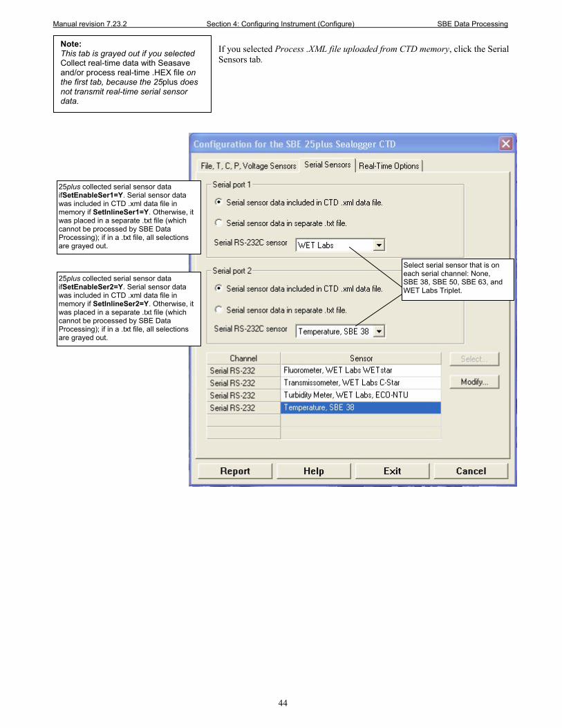
Manual revision 7.23.2 Section 4: Configuring Instrument (Configure) SBE Data Processing
44
If you selected Process .XML file uploaded from CTD memory, click the Serial Sensors tab.
Note: This tab is grayed out if you selected Collect real-time data with Seasave and/or process real-time .HEX file on the first tab, because the 25plus does not transmit real-time serial sensor data.
25plus collected serial sensor data ifSetEnableSer1=Y. Serial sensor data was included in CTD .xml data file in memory if SetInlineSer1=Y. Otherwise, it was placed in a separate .txt file (which cannot be processed by SBE Data Processing); if in a .txt file, all selections are grayed out.
25plus collected serial sensor data ifSetEnableSer2=Y. Serial sensor data was included in CTD .xml data file in memory if SetInlineSer2=Y. Otherwise, it was placed in a separate .txt file (which cannot be processed by SBE Data Processing); if in a .txt file, all selections are grayed out.
Select serial sensor that is on each serial channel: None, SBE 38, SBE 50, SBE 63, and WET Labs Triplet.
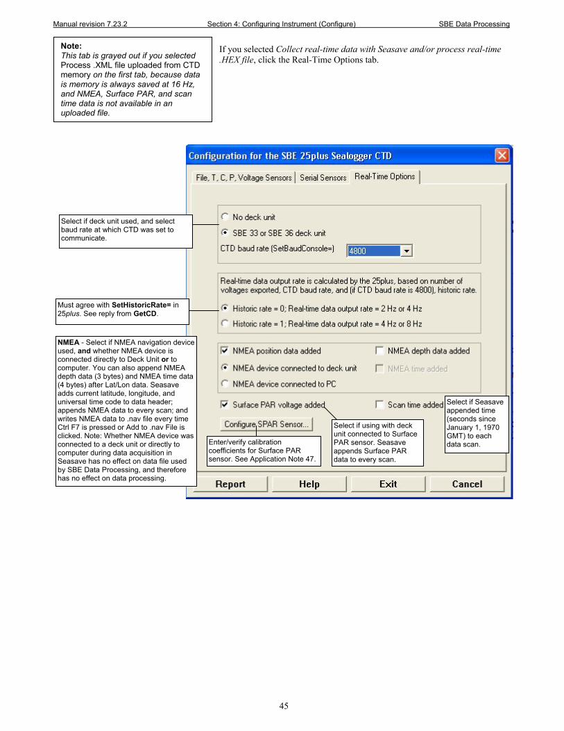
Manual revision 7.23.2 Section 4: Configuring Instrument (Configure) SBE Data Processing
45
If you selected Collect real-time data with Seasave and/or process real-time .HEX file, click the Real-Time Options tab.
Note: This tab is grayed out if you selected Process .XML file uploaded from CTD memory on the first tab, because data is memory is always saved at 16 Hz, and NMEA, Surface PAR, and scan time data is not available in an uploaded file.
Must agree with SetHistoricRate= in 25plus. See reply from GetCD.
NMEA - Select if NMEA navigation device used, and whether NMEA device is connected directly to Deck Unit or to computer. You can also append NMEA depth data (3 bytes) and NMEA time data (4 bytes) after Lat/Lon data. Seasave adds current latitude, longitude, and universal time code to data header; appends NMEA data to every scan; and writes NMEA data to .nav file every time Ctrl F7 is pressed or Add to .nav File is clicked. Note: Whether NMEA device was connected to a deck unit or directly to computer during data acquisition in Seasave has no effect on data file used by SBE Data Processing, and therefore has no effect on data processing.
Select if Seasave appended time (seconds since January 1, 1970 GMT) to each data scan.
Select if using with deck unit connected to Surface PAR sensor. Seasave appends Surface PAR data to every scan.
Enter/verify calibration coefficients for Surface PAR sensor. See Application Note 47.
Select if deck unit used, and select baud rate at which CTD was set to communicate.
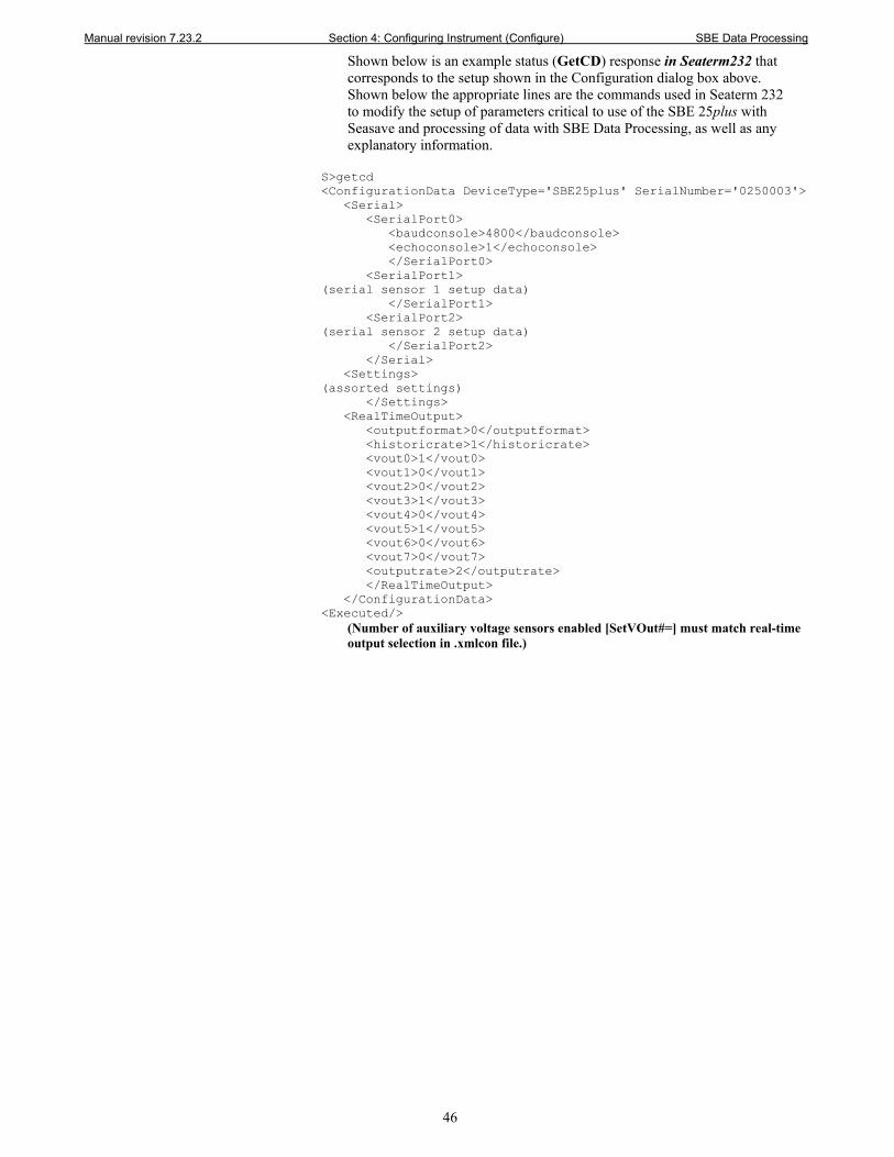
Manual revision 7.23.2 Section 4: Configuring Instrument (Configure) SBE Data Processing
46
Shown below is an example status (GetCD) response in Seaterm232 that corresponds to the setup shown in the Configuration dialog box above. Shown below the appropriate lines are the commands used in Seaterm 232 to modify the setup of parameters critical to use of the SBE 25plus with Seasave and processing of data with SBE Data Processing, as well as any explanatory information.
S>getcd <ConfigurationData DeviceType='SBE25plus' SerialNumber='0250003'> <Serial> <SerialPort0> <baudconsole>4800</baudconsole> <echoconsole>1</echoconsole> </SerialPort0> <SerialPort1> (serial sensor 1 setup data) </SerialPort1> <SerialPort2> (serial sensor 2 setup data) </SerialPort2> </Serial> <Settings> (assorted settings) </Settings> <RealTimeOutput> <outputformat>0</outputformat> <historicrate>1</historicrate> <vout0>1</vout0> <vout1>0</vout1> <vout2>0</vout2> <vout3>1</vout3> <vout4>0</vout4> <vout5>1</vout5> <vout6>0</vout6> <vout7>0</vout7> <outputrate>2</outputrate> </RealTimeOutput> </ConfigurationData> <Executed/>
(Number of auxiliary voltage sensors enabled [SetVOut#=] must match real-time output selection in .xmlcon file.)
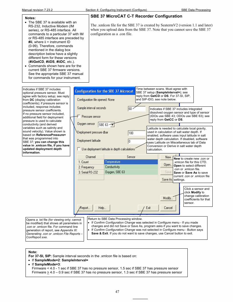
Manual revision 7.23.2 Section 4: Configuring Instrument (Configure) SBE Data Processing
47
SBE 37 MicroCAT C-T Recorder Configuration
The .xmlcon file for the SBE 37 is created by SeatermV2 (version 1.1 and later) when you upload data from the SBE 37. Note that you cannot save the SBE 37 configuration as a .con file.
Notes: • The SBE 37 is available with an
RS-232, Inductive Modem (IM series), or RS-485 interface. All commands to a particular 37 with IM or RS-485 interface are preceded by #ii, where ii = instrument ID (0-99). Therefore, commands mentioned in the dialog box description below have a slightly different form for these versions (#iiGetCD, #iiDS, #iiDC, etc.).
• Commands shown here are for the current SBE 37 firmware versions. See the appropriate SBE 37 manual for commands for your instrument.
Note: For 37-SI, SIP: Sample interval seconds in the .xmlcon file is based on: • If SampleMode=2: SampleInterval= • If SampleMode=3:
Firmware < 4.0 - 1 sec if SBE 37 has no pressure sensor, 1.5 sec if SBE 37 has pressure sensor Firmware > 4.0 – 0.9 sec if SBE 37 has no pressure sensor, 1.3 sec if SBE 37 has pressure sensor
Click a sensor and click Modify to change calibration coefficients for that sensor.
New to create new .con or .xmlcon file for this CTD. Open to select different .con or .xmlcon file. Save or Save As to save current .con or .xmlcon file settings.
Indicates if SBE 37 includes integrated dissolved oxygen sensor and type of sensor (IDOs use SBE 43; ODOs use SBE 63); see reply from GetCC or DS.
Return to SBE Data Processing window. • If Confirm Configuration Change was selected in Configure menu - If you made
changes and did not Save or Save As, program asks if you want to save changes. • If Confirm Configuration Change was not selected in Configure menu - Button says
Save & Exit. If you do not want to save changes, use Cancel button to exit.
Latitude is needed to calculate local gravity, used in calculation of salt water depth. If enabled, software uses input latitude in salt water depth calculation. If disabled, software uses Latitude on Miscellaneous tab of Data Conversion or Derive in salt water depth calculation.
Time between scans. Must agree with SBE 37 setup (SampleInterval=); see reply from GetCD or DS. For 37-SI, SIP, and SIP-IDO, see note below.
Indicates if SBE 37 includes optional pressure sensor. Must agree with factory setup; see reply from DC (display calibration coefficients); if pressure sensor is included, response includes pressure sensor coefficients. If no pressure sensor included, additional field for deployment pressure is used to calculate conductivity (and derived variables such as salinity and sound velocity). Value shown is based on ReferencePressure= that was programmed into SBE 37; you can change this value in .xmlcon file, if you have updated deployment depth information.
Opens a .txt file (for viewing only; cannot be modified) that shows all parameters in .con or .xmlcon file. For command line generation of report, see Appendix III: Generating .con or .xmlcon File Reports – ConReport.exe.

Manual revision 7.23.2 Section 4: Configuring Instrument (Configure) SBE Data Processing
48
Shown below is an example status (DS) response in a terminal program for a SBE 37-SMP-IDO with standard RS-232 interface that corresponds to the setup shown in the Configuration dialog box above. Shown below the appropriate lines are the commands used in the terminal program to modify the setup of parameters critical processing of to SBE 37-SMP-IDO data with SBE Data Processing, as well as any explanatory information.
SBE37SMP-ODO-232 1.0 SERIAL NO. 12345 20 Sep 2012 00:48:50 (‘IDO’ indicates MicroCAT includes integrated oxygen sensor; must match oxygen sensor enable/disable in .xmlcon file.) vMain = 13.31, vLith = 3.19 samplenumber = 1728, free = 522560 not logging, stop command sample interval = 60 seconds (Sample interval [SampleInterval=] must match Sample interval seconds in .xmlcon file.) data format = converted engineering transmit real-time data = yes sync mode = no minimum conductivity frequency = 3000.0 adaptive pump control enabled
If no pressure sensor is installed, a line in the DS response provides user-input reference pressure information; if the pressure sensor is installed, that line is missing (as shown in the above example response). This must match the pressure sensor enable/disable in the .xmlcon file.
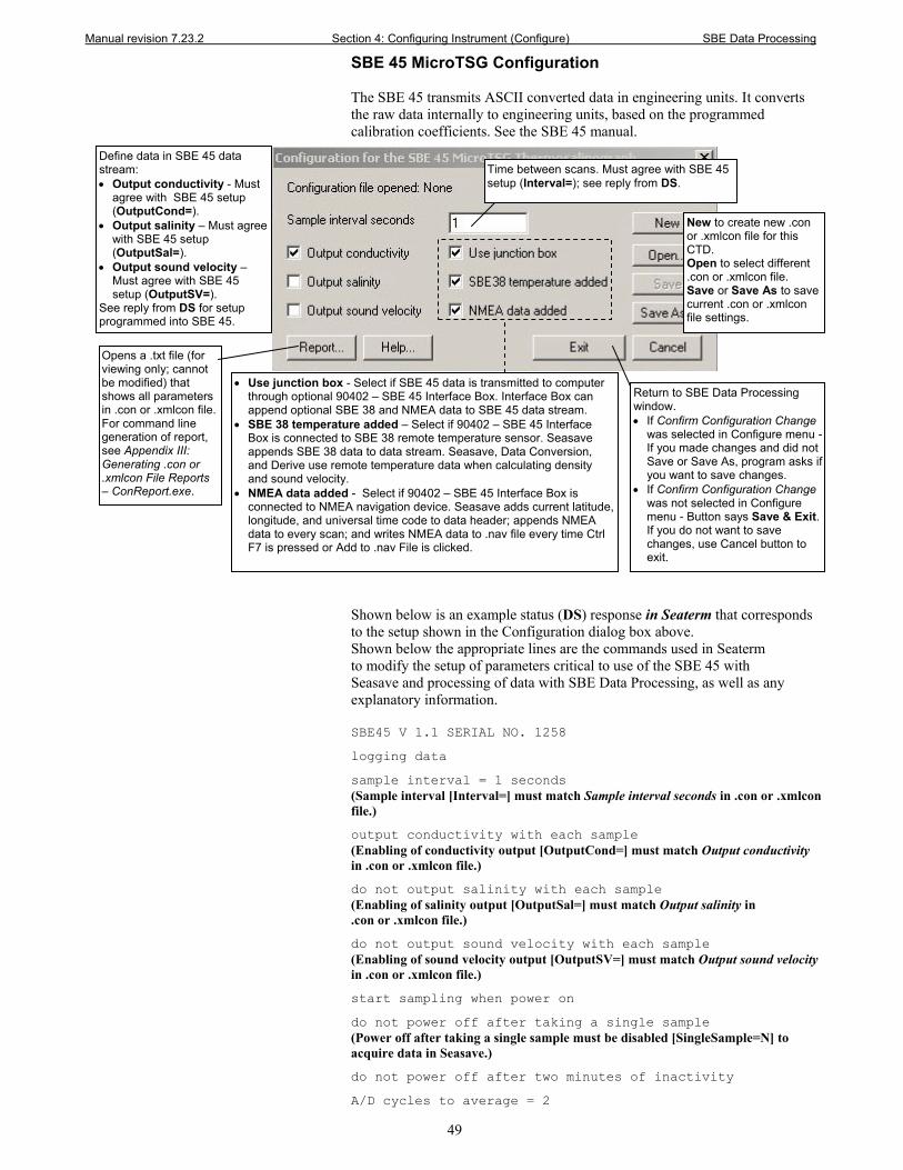
Manual revision 7.23.2 Section 4: Configuring Instrument (Configure) SBE Data Processing
49
SBE 45 MicroTSG Configuration
The SBE 45 transmits ASCII converted data in engineering units. It converts the raw data internally to engineering units, based on the programmed calibration coefficients. See the SBE 45 manual.
Shown below is an example status (DS) response in Seaterm that corresponds to the setup shown in the Configuration dialog box above. Shown below the appropriate lines are the commands used in Seaterm to modify the setup of parameters critical to use of the SBE 45 with Seasave and processing of data with SBE Data Processing, as well as any explanatory information. SBE45 V 1.1 SERIAL NO. 1258
logging data
sample interval = 1 seconds (Sample interval [Interval=] must match Sample interval seconds in .con or .xmlcon file.)
output conductivity with each sample (Enabling of conductivity output [OutputCond=] must match Output conductivity in .con or .xmlcon file.)
do not output salinity with each sample (Enabling of salinity output [OutputSal=] must match Output salinity in .con or .xmlcon file.)
do not output sound velocity with each sample (Enabling of sound velocity output [OutputSV=] must match Output sound velocity in .con or .xmlcon file.)
start sampling when power on
do not power off after taking a single sample (Power off after taking a single sample must be disabled [SingleSample=N] to acquire data in Seasave.)
do not power off after two minutes of inactivity
A/D cycles to average = 2
Define data in SBE 45 data stream: • Output conductivity - Must
agree with SBE 45 setup (OutputCond=).
• Output salinity – Must agree with SBE 45 setup (OutputSal=).
• Output sound velocity – Must agree with SBE 45 setup (OutputSV=).
See reply from DS for setup programmed into SBE 45.
• Use junction box - Select if SBE 45 data is transmitted to computer through optional 90402 – SBE 45 Interface Box. Interface Box can append optional SBE 38 and NMEA data to SBE 45 data stream.
• SBE 38 temperature added – Select if 90402 – SBE 45 Interface Box is connected to SBE 38 remote temperature sensor. Seasave appends SBE 38 data to data stream. Seasave, Data Conversion, and Derive use remote temperature data when calculating density and sound velocity.
• NMEA data added - Select if 90402 – SBE 45 Interface Box is connected to NMEA navigation device. Seasave adds current latitude, longitude, and universal time code to data header; appends NMEA data to every scan; and writes NMEA data to .nav file every time Ctrl F7 is pressed or Add to .nav File is clicked.
New to create new .con or .xmlcon file for this CTD. Open to select different .con or .xmlcon file. Save or Save As to save current .con or .xmlcon file settings.
Return to SBE Data Processing window. • If Confirm Configuration Change
was selected in Configure menu - If you made changes and did not Save or Save As, program asks if you want to save changes.
• If Confirm Configuration Change was not selected in Configure menu - Button says Save & Exit. If you do not want to save changes, use Cancel button to exit.
Time between scans. Must agree with SBE 45 setup (Interval=); see reply from DS.
Opens a .txt file (for viewing only; cannot be modified) that shows all parameters in .con or .xmlcon file. For command line generation of report, see Appendix III: Generating .con or .xmlcon File Reports – ConReport.exe.
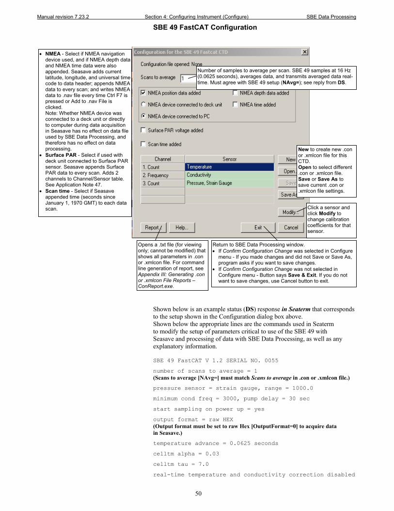
Manual revision 7.23.2 Section 4: Configuring Instrument (Configure) SBE Data Processing
50
SBE 49 FastCAT Configuration
Shown below is an example status (DS) response in Seaterm that corresponds to the setup shown in the Configuration dialog box above. Shown below the appropriate lines are the commands used in Seaterm to modify the setup of parameters critical to use of the SBE 49 with Seasave and processing of data with SBE Data Processing, as well as any explanatory information. SBE 49 FastCAT V 1.2 SERIAL NO. 0055
number of scans to average = 1 (Scans to average [NAvg=] must match Scans to average in .con or .xmlcon file.)
pressure sensor = strain gauge, range = 1000.0
minimum cond freq = 3000, pump delay = 30 sec
start sampling on power up = yes
output format = raw HEX (Output format must be set to raw Hex [OutputFormat=0] to acquire data in Seasave.)
temperature advance = 0.0625 seconds
celltm alpha = 0.03
celltm tau = 7.0
real-time temperature and conductivity correction disabled
Number of samples to average per scan. SBE 49 samples at 16 Hz (0.0625 seconds), averages data, and transmits averaged data real-time. Must agree with SBE 49 setup (NAvg=); see reply from DS.
Click a sensor and click Modify to change calibration coefficients for that sensor.
New to create new .con or .xmlcon file for this CTD. Open to select different .con or .xmlcon file. Save or Save As to save current .con or .xmlcon file settings.
Return to SBE Data Processing window. • If Confirm Configuration Change was selected in Configure
menu - If you made changes and did not Save or Save As, program asks if you want to save changes.
• If Confirm Configuration Change was not selected in Configure menu - Button says Save & Exit. If you do not want to save changes, use Cancel button to exit.
• NMEA - Select if NMEA navigation device used, and if NMEA depth data and NMEA time data were also appended. Seasave adds current latitude, longitude, and universal time code to data header; appends NMEA data to every scan; and writes NMEA data to .nav file every time Ctrl F7 is pressed or Add to .nav File is clicked. Note: Whether NMEA device was connected to a deck unit or directly to computer during data acquisition in Seasave has no effect on data file used by SBE Data Processing, and therefore has no effect on data processing.
• Surface PAR - Select if used with deck unit connected to Surface PAR sensor. Seasave appends Surface PAR data to every scan. Adds 2 channels to Channel/Sensor table. See Application Note 47.
• Scan time - Select if Seasave appended time (seconds since January 1, 1970 GMT) to each data scan.
Opens a .txt file (for viewing only; cannot be modified) that shows all parameters in .con or .xmlcon file. For command line generation of report, see Appendix III: Generating .con or .xmlcon File Reports – ConReport.exe.
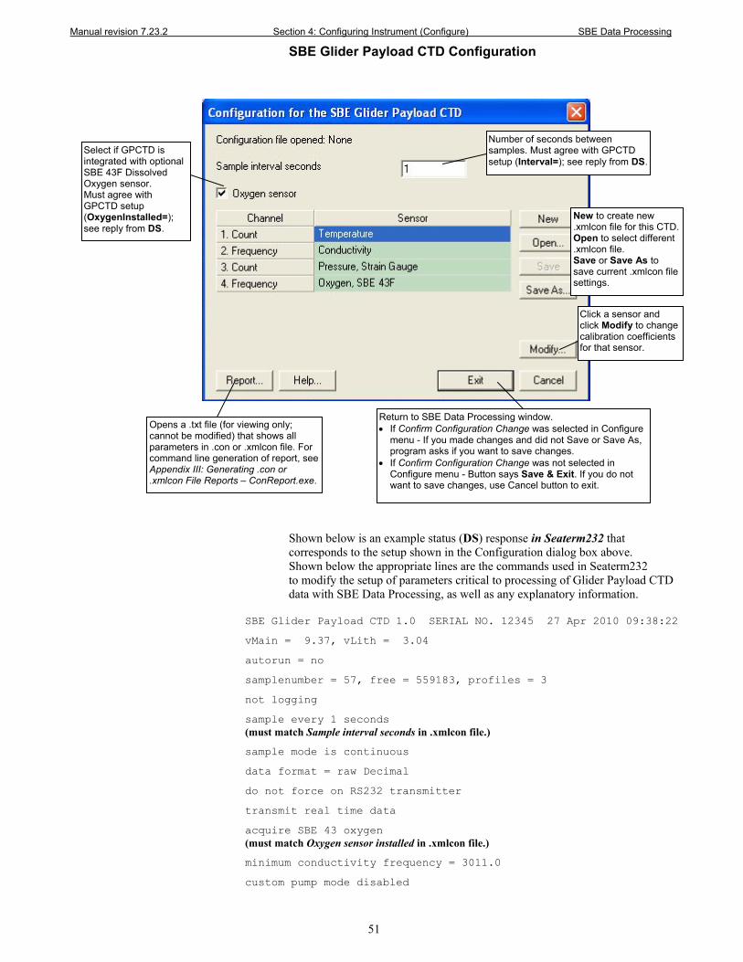
Manual revision 7.23.2 Section 4: Configuring Instrument (Configure) SBE Data Processing
51
SBE Glider Payload CTD Configuration
Shown below is an example status (DS) response in Seaterm232 that corresponds to the setup shown in the Configuration dialog box above. Shown below the appropriate lines are the commands used in Seaterm232 to modify the setup of parameters critical to processing of Glider Payload CTD data with SBE Data Processing, as well as any explanatory information.
SBE Glider Payload CTD 1.0 SERIAL NO. 12345 27 Apr 2010 09:38:22
vMain = 9.37, vLith = 3.04
autorun = no
samplenumber = 57, free = 559183, profiles = 3
not logging
sample every 1 seconds (must match Sample interval seconds in .xmlcon file.)
sample mode is continuous
data format = raw Decimal
do not force on RS232 transmitter
transmit real time data
acquire SBE 43 oxygen (must match Oxygen sensor installed in .xmlcon file.)
minimum conductivity frequency = 3011.0
custom pump mode disabled
Click a sensor and click Modify to change calibration coefficients for that sensor.
New to create new .xmlcon file for this CTD. Open to select different .xmlcon file. Save or Save As to save current .xmlcon file settings.
Return to SBE Data Processing window. • If Confirm Configuration Change was selected in Configure
menu - If you made changes and did not Save or Save As, program asks if you want to save changes.
• If Confirm Configuration Change was not selected in Configure menu - Button says Save & Exit. If you do not want to save changes, use Cancel button to exit.
Select if GPCTD is integrated with optional SBE 43F Dissolved Oxygen sensor. Must agree with GPCTD setup (OxygenInstalled=); see reply from DS.
Opens a .txt file (for viewing only; cannot be modified) that shows all parameters in .con or .xmlcon file. For command line generation of report, see Appendix III: Generating .con or .xmlcon File Reports – ConReport.exe.
Number of seconds between samples. Must agree with GPCTD setup (Interval=); see reply from DS.
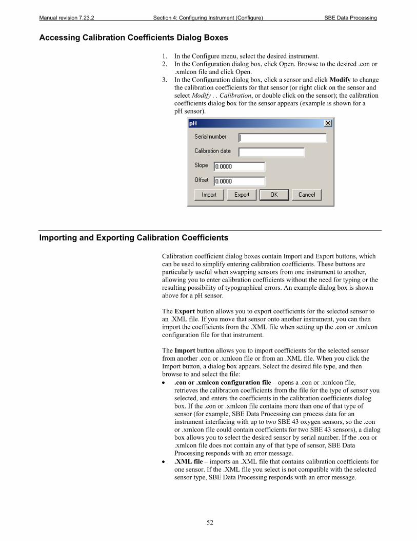
Manual revision 7.23.2 Section 4: Configuring Instrument (Configure) SBE Data Processing
52
Accessing Calibration Coefficients Dialog Boxes 1. In the Configure menu, select the desired instrument. 2. In the Configuration dialog box, click Open. Browse to the desired .con or
.xmlcon file and click Open. 3. In the Configuration dialog box, click a sensor and click Modify to change
the calibration coefficients for that sensor (or right click on the sensor and select Modify . . Calibration, or double click on the sensor); the calibration coefficients dialog box for the sensor appears (example is shown for a pH sensor).
Importing and Exporting Calibration Coefficients
Calibration coefficient dialog boxes contain Import and Export buttons, which can be used to simplify entering calibration coefficients. These buttons are particularly useful when swapping sensors from one instrument to another, allowing you to enter calibration coefficients without the need for typing or the resulting possibility of typographical errors. An example dialog box is shown above for a pH sensor. The Export button allows you to export coefficients for the selected sensor to an .XML file. If you move that sensor onto another instrument, you can then import the coefficients from the .XML file when setting up the .con or .xmlcon configuration file for that instrument. The Import button allows you to import coefficients for the selected sensor from another .con or .xmlcon file or from an .XML file. When you click the Import button, a dialog box appears. Select the desired file type, and then browse to and select the file: • .con or .xmlcon configuration file – opens a .con or .xmlcon file,
retrieves the calibration coefficients from the file for the type of sensor you selected, and enters the coefficients in the calibration coefficients dialog box. If the .con or .xmlcon file contains more than one of that type of sensor (for example, SBE Data Processing can process data for an instrument interfacing with up to two SBE 43 oxygen sensors, so the .con or .xmlcon file could contain coefficients for two SBE 43 sensors), a dialog box allows you to select the desired sensor by serial number. If the .con or .xmlcon file does not contain any of that type of sensor, SBE Data Processing responds with an error message.
• .XML file – imports an .XML file that contains calibration coefficients for one sensor. If the .XML file you select is not compatible with the selected sensor type, SBE Data Processing responds with an error message.
Manual revision 7.23.2 Section 4: Configuring Instrument (Configure) SBE Data Processing
53
Calibration Coefficients for Frequency Sensors
View and/or modify the sensor calibration coefficients by selecting the sensor and clicking the Modify button in the instrument Configuration dialog box. For all calibration dialog boxes, enter the sensor serial number and calibration date. Many sensor calibration equations contain an offset term. Unless noted otherwise, use the offset (default = 0.0) to make small corrections for sensor drift between calibrations. Calibration coefficients are discussed below for each type of sensor. Temperature, conductivity, and Digiquartz pressure sensors are covered first, followed by the remaining frequency sensor types in alphabetical order. Temperature Calibration Coefficients Enter g, h, i, j (or a, b, c, d), and f0 from the calibration sheet. Enter values for slope (default = 1.0) and offset (default = 0.0) to make small corrections for temperature sensor drift between calibrations:
Corrected temperature = (slope * computed temperature) + offset where slope = true temperature span / instrument temperature span offset = (true temperature – instrument reading) * slope; measured at 0 °C
Temperature Slope and Offset Correction Example At true temperature = 0.0 °C, instrument reading = 0.0015 °C At true temperature = 25.0 °C, instrument reading = 25.0005 °C Calculating the slope and offset: Slope = (25.0 – 0.0) / (25.0005 – 0.0015) = + 1.000040002 Offset = (0.0 – 0.0015) * 1.000040002 = - 0.001500060
Sea-Bird temperature sensors usually drift by changing offset, typically resulting in higher temperature readings over time for sensors with serial number less than 1050 and lower temperature readings over time for sensors with serial number greater than 1050. Sea-Bird’s data indicates that the drift is smooth and uniform with time, allowing users to make very accurate corrections based only on pre- and post-cruise laboratory calibrations. Calibration checks at sea are advisable to ensure against sensor malfunction; however, data from reversing thermometers is rarely accurate enough to make calibration corrections that are better than those possible from shore-based laboratory calibrations. Sea-Bird temperature sensors rarely exhibit span errors larger than ± 0.005 °C over the range –5 to +35 °C (0.005 °C/(35 -[-5])C/year = 0.000125 °C/C/year), even after years of drift. A span error that increases more than ± 0.0002 °C/C/year may be a symptom of sensor malfunction.
Notes: • Coefficients g, h, i, j, and f0
provide ITS-90 (T90) temperature; a, b, c, d, and f0 provide IPTS-68 (T68) temperature. The relationship between them is: T68 = 1.00024 T90
• See Application Note 31 for computation of slope and offset correction coefficients from pre- and post-cruise calibrations supplied by Sea-Bird.
• See Calibration Coefficients for A/D Count Sensors below for information on temperature sensors used in the SBE 16plus (and -IM), 16plus (and -IM) V2, 19plus, 19plus V2, 37, and 49.
Manual revision 7.23.2 Section 4: Configuring Instrument (Configure) SBE Data Processing
54
Conductivity Calibration Coefficients Enter g, h, i, j, Ctcor (or a, b, c, d, m) and Cpcor from the calibration sheet. • Cpcor makes a correction for the highly consistent change in dimensions of
the conductivity cell under pressure. The default is the compressibility coefficient for borosilicate glass (-9.57e-08). Some sensors fabricated between 1992 and 1995 (serial numbers between 1100 and 1500) exhibit a compression that is slightly less than pure borosilicate glass. For these sensors, the (hermetic) epoxy jacket on the glass cell is unintentionally strong, creating a composite pressure effect of borosilicate and epoxy. For sensors tested to date, this composite pressure coefficient ranges from -9.57e-08 to -6.90e-08, with the latter value producing a correction to deep ocean salinity of 0.0057 PSU in 5000 dbars pressure (approximately 0.001 PSU per 1000 dbars). Before modifying Cpcor, confirm that the sensor behaves differently from pure borosilicate glass. Sea-Bird can test your cell and calculate Cpcor. Alternatively, test the cell by comparing computed salinity to the salinity of water samples from a range of depths, calculated using an AutoSal.
Enter values for slope (default = 1.0) and offset (default = 0.0) to make small corrections for conductivity sensor drift between calibrations:
Corrected conductivity = (slope * computed conductivity) + offset where slope = true conductivity span / instrument conductivity span offset = (true conductivity – instrument reading) * slope; measured at 0 S/m
Conductivity Slope and Offset Correction Example At true conductivity = 0.0 S/m, instrument reading = -0.00007 S/m At true conductivity = 3.5 S/m, instrument reading = 3.49965 S/m Calculating the slope and offset: Slope = (3.5 – 0.0) / (3.49965 - [- 0.00007]) = + 1.000080006 Offset = (0.0 - [-0.00007]) * 1.000080006 = + 0.000070006
The sensor usually drifts by changing span (slope of the calibration curve), typically resulting in lower conductivity readings over time. Offset error (error at 0 S/m) is usually due to electronics drift, and is typically less than ± 0.0001 S/m per year. Because offsets greater than ± 0.0002 S/m are a symptom of sensor malfunction, Sea-Bird recommends that drift corrections be made by assuming no offset error, unless there is strong evidence to the contrary or a special need. Wide-Range Conductivity Sensors A wide-range conductivity sensor has been modified to provide conductivity readings over a wider range by inserting a precision resistor in series with the conductivity cell. Therefore, the equation used to fit the calibration data is different from the standard equation. The sensor’s documentation includes the equation as well as the cell constant and series resistance to be entered in the program. If the conductivity sensor serial number on the conductivity calibration sheet includes a w (an indication that it is a wide-range sensor; for example, 4216w): 1. After you enter the calibration coefficients and click OK, the Wide Range
Conductivity dialog box appears. 2. Enter the cell constant and series resistance (from the instrument’s
documentation) in the dialog box, and click OK.
Note: See Application Note 31 for computation of slope and offset correction coefficients from pre- and post-cruise calibrations supplied by Sea-Bird or from salinity bottle samples taken at sea during profiling.
Note: Use coefficients g, h, i, j, Ctcor, and Cpcor (if available on calibration sheet) for most accurate results; conductivity for older sensors was calculated based on a, b, c, d, m, and Cpcor.
Note: See Application Note 94 for information on wide-range calibrations.
Manual revision 7.23.2 Section 4: Configuring Instrument (Configure) SBE Data Processing
55
Pressure (Paroscientific Digiquartz) Calibration Coefficients Enter the sets of C, D, and T coefficients from the calibration sheet. Enter zero for any higher-order coefficients that are not listed on the calibration sheet. Enter values for slope (default = 1.0; do not change unless sensor has been recalibrated) and offset (default = 0.0) to make small corrections for sensor drift. • For the SBE 9plus, also enter AD590M and AD590B coefficients from the
configuration sheet. Oxygen (SBE 43I) Calibration Coefficients The SBE 43I is the Integrated Dissolved Oxygen sensor used on the SBE 37 (37-SMP-IDO, 37-IMP-IDO, and 37-SIP-IDO). The calibration coefficients for this sensor are as described for the SBE 43 voltage sensor (see Calculation Coefficients for Voltage Sensors below). Bottles Closed (HB - IOW) Calibration Coefficients No calibration coefficients are entered for this parameter. The number of bottles closed is calculated by Data Conversion based on frequency range. Sound Velocity (IOW) Calibration Coefficients Enter coefficients a0, a1, and a2. Value = a0 + a1 * frequency + a2 * frequency 2
Note: See Calibration Coefficients for A/D Count Sensors below for information on strain gauge pressure sensors used on the SBE 16plus (and -IM), 16plus (and -IM) V2, 19plus, 19plus V2, and 49. See Calibration Coefficients for Voltage Sensors below for information on strain gauge pressure sensors used on other instruments.
Manual revision 7.23.2 Section 4: Configuring Instrument (Configure) SBE Data Processing
56
Calibration Coefficients for A/D Count Sensors
View and/or modify the sensor calibration coefficients by selecting the sensor and clicking the Modify button in the instrument Configuration dialog box. For all calibration dialog boxes, enter the sensor serial number and calibration date. Many sensor calibration equations contain an offset term. Unless noted otherwise, use the offset (default = 0.0) to make small corrections for sensor drift between calibrations. Calibration coefficients are discussed below for each type of sensor: temperature and strain gauge pressure sensor. Temperature Calibration Coefficients For SBE 16plus (and -IM), 16plus (and-IM) V2, 19plus, 19plus V2, 37, and 49: Enter a0, a1, a2, and a3 from the calibration sheet. Enter values for slope (default = 1.0) and offset (default = 0.0) to make small corrections for temperature sensor drift between calibrations:
Corrected temperature = (slope * computed temperature) + offset where slope = true temperature span / instrument temperature span offset = (true temperature – instrument reading) * slope; measured at 0 °C
Temperature Slope and Offset Correction Example At true temperature = 0.0 °C, instrument reading = 0.0015 °C At true temperature = 25.0 °C, instrument reading = 25.0005 °C Calculating the slope and offset: Slope = (25.0 – 0.0) / (25.0005 – 0.0015) = + 1.000040002 Offset = (0.0 – 0.0015) * 1.000040002 = - 0.001500060
Sea-Bird temperature sensors usually drift by changing offset, typically resulting in lower temperature readings over time. Sea-Bird’s data indicates that the drift is smooth and uniform with time, allowing users to make very accurate corrections based only on pre- and post-cruise laboratory calibrations. Calibration checks at sea are advisable to ensure against sensor malfunction; however, data from reversing thermometers is rarely accurate enough to make calibration corrections that are better than those possible from shore-based laboratory calibrations. Sea-Bird temperature sensors rarely exhibit span errors larger than ± 0.005 °C over the range –5 to +35 °C (0.005 °C/(35 -[-5])C/year = 0.000125 °C/C/year), even after years of drift. A span error that increases more than ± 0.0002 °C/C/year may be a symptom of sensor malfunction. Pressure (Strain Gauge) Calibration Coefficients For SBE 16plus (and -IM), 16plus (and IM) V2, 19plus, and 19plus V2 configured with a strain gauge pressure sensor, and for all SBE 37s and 49s: Enter pA0, pA1, pA2, ptempA0, ptempA1, ptempA2, pTCA0, pTCA1, pTCA2, pTCB0, pTCB1, and pTCB2 from the calibration sheet. Offset is normally zero, but may be changed for non-zero sea-surface condition. For example, if the in-air pressure reading is negative, enter an equal positive value.
Notes: • These coefficients provide
ITS-90 (T90) temperature. • See Application Note 31 for
computation of slope and offset correction coefficients from pre- and post-cruise calibrations supplied by Sea-Bird.
Note: See Calibration Coefficients for Voltage Sensors below for information on strain gauge pressure sensors used on other instruments. See Calibration Coefficients for Frequency Sensors above for information on Paroscientific Digiquartz pressure sensors.
Manual revision 7.23.2 Section 4: Configuring Instrument (Configure) SBE Data Processing
57
Calibration Coefficients for Voltage Sensors
View and/or modify the sensor calibration coefficients by selecting the sensor and clicking the Modify button in the instrument Configuration dialog box. For all calibration dialog boxes, enter the sensor serial number and calibration date. Many sensor calibration equations contain an offset term. Unless noted otherwise, use the offset (default = 0.0) to make small corrections for sensor drift between calibrations. Calibration coefficients are discussed below for each type of sensor. Strain gauge pressure sensors are covered first, followed by the remaining voltage sensor types in alphabetical order. Pressure (Strain Gauge) Calibration Coefficients Enter coefficients: • Pressure sensor without temperature compensation
Enter A0, A1, and A2 coefficients from the calibration sheet For older units with a linear fit pressure calibration, enter M (A1) and
B (A0) from the calibration sheet, and set A2 to zero. For all units, offset is normally zero, but may be changed for non-zero
sea-surface condition. For example, if the in-air pressure reading is negative, enter an equal positive value.
• Pressure sensor with temperature compensation Enter ptempA0, ptempA1, ptempA2, pTCA0, pTCA1, pTCA2, pTCB0, pTCB1, pTCB2, pA0, pA1, and pA2 from the calibration sheet.
Altimeter Calibration Coefficients Enter the scale factor and offset. altimeter height = [300 * voltage / scale factor] + offset where scale factor = full scale voltage * 300/full scale range full scale range is dependent on the sensor (e.g., 50m, 100m, etc.) full scale voltage is from calibration sheet (typically 5V) Fluorometer Calibration Coefficients • Biospherical Natural Fluorometer
Enter Cfn (natural fluorescence calibration coefficient), A1, A2, and B from calibration sheet. natural fluorescence Fn = Cfn * 10V production = A1 * Fn / (A2 + PAR) chlorophyll concentration Chl = Fn / (B * PAR) where V is voltage from natural fluorescence sensor
Note: In Seasave, enter the altimeter alarm set point, alarm hysteresis, and minimum pressure to enable alarm.
Note: See Calibration Coefficients for A/D Count Sensors above for information on strain gauge pressure sensors used on the SBE 16plus (and -IM), 16plus (and -IM) V2, 19plus, 19plus V2, and 49. See Calibration Coefficients for Frequency Sensors above for information on Paroscientific Digiquartz pressure sensors.
Note: Unless noted otherwise, SBE Data Processing supports only one of each auxiliary sensor model on a CTD (for example, you cannot specify two Chelsea Minitracka fluorometers, but you can specify a Chelsea Minitracka and a Chelsea UV Aquatracka fluorometer. See the sensor descriptions below for those sensors that SBE Data Processing supports in a redundant configuration (two or more of the same model interfacing with the CTD).
Manual revision 7.23.2 Section 4: Configuring Instrument (Configure) SBE Data Processing
58
• Chelsea Aqua 3 Enter VB, V1, Vacetone, slope, offset, and SF. Concentration (μg/l) = slope*[(10.0(V/SF) - 10.0VB)/(10.0V1 - 10.0Vacetone)]
+ offset where VB, V1, and Vacetone are from calibration sheet Slope (default 1.0) and offset (default 0.0) adjust readings to conform to measured concentrations Scale factor SF = 1.0 if CTD gain is 1; SF = 2 if CTD gain is 2.0 V is output voltage measured by CTD Note: SBE Data Processing can process data for an instrument interfacing with up to two Chelsea Aqua 3 fluorometers.
Chelsea Aqua 3 Example - Calculation of Slope and Offset Current slope = 1.0 and offset = 0.0 Two in-situ samples:
Sample 1 Concentration– from SBE Data Processing = 0.390, from water sample = 0.450 Sample 2 Concentration– from SBE Data Processing = 0.028, from water sample = 0.020
Linear regression to this data yields slope = 1.188 and offset = - 0.013
• Chelsea Minitracka Enter Vacetone, Vacetone100, and offset. Concentration = (100 *[V - Vacetone]/[Vacetone100 - Vacetone]) + offset where Vacetone (voltage with 0 µg/l chlorophyll) and Vacetone100 (voltage with 100 µg/l chlorophyll) are from calibration sheet
• Chelsea UV Aquatracka Enter A and B. Concentration (μg/l) = A * 10.0 V - B where A and B are from calibration sheet V is output voltage measured by CTD Note: SBE Data Processing can process data for an instrument interfacing with up to two Chelsea UV Aquatracka fluorometers.
• Dr Haardt Fluorometer - Chlorophyll a, Phycoerythrin, or
Yellow Substance Enter A0, A1, B0, and B1. These instruments may have automatic switching between high and low gains. Select the gain range switch: Output Voltage Level if the instrument indicates gain by output voltage
level (< 2.5 volts is low gain, > 2.5 volts is high gain) Low gain: value = A0 + (A1 * V) High gain: value = B0 + (B1 * V)
Modulo Bit if the instrument has control lines custom-wired to bits in the SBE 9plus modulo word Bit not set: value = A0 + (A1 * V) Bit set: value = B0 + (B1 * V)
None if the instrument does not change gain value = A0 + (A1 * V)
where V = voltage from sensor
Dr Haardt Voltage Level Switching Examples Example: Chlorophyll a Low range scale = 10 mg/l and Gain = 10/2.5 = 4 mg/l/volt A0 = 0.0 A1 = 4.0 High range scale = 100 mg/l and Gain = 100/2.5 = 40 mg/l/volt B0 = -100 B1 = 40.0
Note: See Application Note 39 for complete description of calculation of Chelsea Aqua 3 calibration coefficients.
Note: See Application Note 61 for complete description of calculation of Chelsea Minitracka calibration coefficients.

Manual revision 7.23.2 Section 4: Configuring Instrument (Configure) SBE Data Processing
59
• Seapoint Enter gain and offset. Concentration = (V * 30/gain) + offset where Gain is dependent on cable used (see cable drawing, pins 5 and 6) Note: SBE Data Processing can process data for an instrument interfacing with up to two Seapoint fluorometers.
• Seapoint Rhodamine
Enter gain and offset. Concentration = (V * 30/gain) + offset where Gain is dependent on cable used (see cable drawing, pins 5 and 6)
• Seapoint Ultraviolet
Enter range and offset. Concentration = (V * range / 5) + offset Note: SBE Data Processing can process data for an instrument interfacing with up to two Seapoint ultraviolet fluorometers.
• Sea Tech and WET Labs Flash Lamp Fluorometer (FLF) Enter scale factor and offset. Concentration = (voltage * scale factor / 5) + offset where Scale factor is dependent on fluorometer range:
Fluorometer Switch-Selectable Range
(milligrams/m3 or micrograms/liter) Scale
Factor
Sea Tech
0 – 3 3 0 – 10 (default) 10
0 - 30 30 0-100 100 0-300 300 0-1000 1000
WET Labs FLF
0 – 100 100 0 – 300 (default) 300
0 - 1000 1000 Offset is calculated by measuring voltage output when the light sensor is completely blocked from the strobe light with an opaque substance such as heavy black rubber: offset = - (scale factor * voltage) / 5
• Turner 10-005 This sensor requires two channels - one for the fluorescence voltage and the other for the range voltage. Make sure to select both when configuring the instrument. For the fluorescence voltage channel, enter scale factor and offset. concentration = [fluorescence voltage * scale factor / (range * 5)] + offset where range is defined in the following table
Range Voltage Range < 0.2 volts 1.0
> 0.2 volts and < 0.55 volts 3.16 > 0.55 volts and < 0.85 volts 10.0
> 0.85 volts 31.0
Note: See Application Note 54 for complete description of calculation of Seapoint fluorometer calibration coefficients.
Notes: • See Application Note 9 for
complete description of calculation of WET Labs FLF and Sea Tech fluorometer calibration coefficients.
• Offset and scale factor may be adjusted to fit a linear regression of fluorometer responses to known chlorophyll a concentrations.
Note: See Application Note 77 for complete description of calculation of Seapoint ultraviolet fluorometer calibration coefficients.
Manual revision 7.23.2 Section 4: Configuring Instrument (Configure) SBE Data Processing
60
• Turner 10-AU-005
Enter full scale voltage, zero point concentration, and full scale concentration from the calibration sheet. concentration = [(1.195 * voltage * (FSC – ZPC)) / FSV] + ZPC where voltage = measured output voltage from fluorometer FSV = full scale voltage; typically 5.0 volts FSC = full scale concentration ZPC = zero point concentration
• Turner Cyclops
Enter scale factor and offset, and select measured parameter (chlorophyll, rhodamine, fluorescein, .phycocyanin, phycoerythrin, CDOM, crude oil, optical brighteners, or turbidity) concentration = (scale factor * voltage) + offset where scale factor = range / 5 volts offset = - scale factor * blank voltage Range and blank voltage are from calibration sheet. Output units are dependent on selected measured parameter. Note: SBE Data Processing can process data for an instrument interfacing with up to two Turner Cyclops fluorometers.
• Turner SCUFA
Enter scale factor, offset, units, mx, my, and b from the calibration sheet. chlorophyll = (scale factor * voltage) + offset corrected chlorophyll = (mx * chlorophyll) + (my * NTU) + b where NTU = results from optional turbidity channel in SCUFA (see Turner SCUFA in OBS equations below) Note: SBE Data Processing can process data for an instrument interfacing with up to two Turner SCUFA sensors.
• WET Labs AC3
This sensor requires two channels - one for fluorometer voltage (listed under fluorometers in the dialog box) and the other for transmissometer voltage (listed under transmissometers). Make sure to select both when configuring the instrument. Enter kv, Vh2o, and A^X. concentration (mg/m3) = kv * (Vout - Vh20) / A^X where Vout = measured output voltage kv = absorption voltage scaling constant (inverse meters/volt) Vh20 = measured voltage using pure water A^X = chlorophyll specific absorption coefficient
Notes: • To enable entry of the mx, my,
and b coefficients, you must first select the Turner SCUFA (OBS/Nephelometer/Turbidity).
• See Application Note 63 for complete description of calculation of Turner SCUFA calibration coefficients.
Note: See Application Note 74 for complete description of calculation of Turner Cyclops fluorometer calibration coefficients.
Manual revision 7.23.2 Section 4: Configuring Instrument (Configure) SBE Data Processing
61
• WET Labs ECO-AFL and ECO-FL Enter Dark Output and scale factor. Concentration (units) = (V – Dark Output) * scale factor where V = in situ voltage output Dark Output = clean water voltage output with black tape on detector Scale factor = multiplier (units/Volt) The calibration sheet lists either: Dark Output and scale factor, OR Vblank (old terminology for Dark Output) and Scale Factor, OR Vblank (old terminology for Dark Output) and Vcopro (voltage output
measured with known concentration of coproporphyrin tetramethyl ester). Determine an initial value for the scale factor by using the chlorophyll concentration corresponding to Vcopro: scale factor = chlorophyll concentration / (Vcopro - Vblank)
Perform calibrations using seawater with phytoplankton populations that are similar to what is expected in situ. Note: SBE Data Processing can process data for an instrument interfacing with up to six ECO-AFL (or ECO-FL) sensors.
• WET Labs ECO CDOM (Colored Dissolved Organic Matter) Enter Dark Output and scale factor. Concentration (ppb) = (V – Dark Output) * Scale Factor where V = in situ voltage output Dark Output = clean water voltage output with black tape on detector Scale Factor = multiplier (ppb/Volt) Calibration sheet lists Dark Output and Vcdom (voltage output measured with known concentration of colored dissolved organic matter). Determine an initial scale factor value by using colored dissolved organic matter concentration corresponding to Vcdom: scale factor = cdom concentration / (Vcdom – Dark Output) Perform calibrations using seawater with CDOM types similar to what is expected in situ. Note: SBE Data Processing can process data for an instrument interfacing with up to six ECO CDOM sensors.
• WET Labs WETStar
Enter Blank Output and Scale Factor. Concentration (units) = (V – Blank Output) * Scale Factor where V = in situ voltage output Blank Output = clean water blank voltage output Scale Factor = multiplier (units/Volt) The calibration sheet lists either: Blank Output and Scale Factor, OR Vblank (old terminology for Blank Output) and Scale Factor, OR Vblank (old terminology for Blank Output) and Vcopro (voltage
output measured with known concentration of coproporphyrin tetramethyl ester). Determine an initial value for the scale factor by using the chlorophyll concentration corresponding to Vcopro: scale factor = chlorophyll concentration / (Vcopro - Vblank)
Perform calibrations using seawater with phytoplankton populations that are similar to what is expected in situ. Note: SBE Data Processing can process data for an instrument interfacing with up to six WET Labs WETStar sensors.
Notes: • Units are dependent on the
substance measured by the fluorometer. For example, units are µg/l for chlorophyll, ppb for Rhodamine, ppt for Phycocyanin, etc.
• For complete description of calibration coefficient calculation, see Application Note 62.
• For ECO-FL-NTU, a second channel is required for turbidity. Set up the second channel as a WET Labs ECO-NTU, as described below for OBS/Nephelometer/Turbidity sensors.
Notes: • Units are dependent on the
substance measured by the fluorometer. For example, units are µg/l for chlorophyll, ppb for Rhodamine, ppt for Phycocyanin, etc.
• For complete description of calibration coefficient calculation, see Application Note 41 for WETStar.

Manual revision 7.23.2 Section 4: Configuring Instrument (Configure) SBE Data Processing
62
Methane Sensor Calibration Coefficients The Franatech(formerly Capsum) METS sensor requires two channels – one for methane concentration and the other for temperature measured by the sensor. Make sure to select both when configuring the instrument. For the concentration channel, enter D, A0, A1, B0, B1, and B2.
Methane concentration = exp {D ln [(B0 + B1 exp ) * ( – )]} [µmol / l]
where Vt = temperature voltage Vm = methane concentration voltage
For the temperature channel, enter T1 and T2. Gas temperature = (Vt * T1) + T2 [°C] OBS/Nephelometer/Turbidity Calibration Coefficients
In general, turbidity sensors are calibrated to a standard (formazin). However, particle size, shape, refraction, etc. in seawater varies. These variations affect the results unless field calibrations are performed on typical water samples.
• Downing & Associates [D&A] OBS-3 Backscatterance Enter gain and offset. output = (volts * gain) + offset where gain = range/5; see calibration sheet for range Note: SBE Data Processing can process data for an instrument interfacing with up to two OBS-3 sensors.
• Downing & Associates [D & A] OBS-3+ Enter A0, A1, and A2. output = A0 + (A1 * V) + (A2 * V2) where V = voltage from sensor (milliVolts) A0, A1, and A2 = calibration coefficients from D & A calibration sheet Note: SBE Data Processing can process data for an instrument interfacing with up to two OBS-3+ sensors.
• Chelsea Enter clear water value and scale factor. turbidity [F.T.U.] = (10.0V – C) / scale factor where V = voltage from sensor See calibration sheet for C (clear water value) and scale factor.
• Dr. Haardt Turbidity Enter A0, A1, B0, and B1. Select the gain range switch: Output Voltage Level if the instrument indicates gain by output voltage
level (< 2.5 volts is low gain, > 2.5 volts is high gain) Low gain: value = A0 + (A1 * V) High gain: value = B0 + (B1 * V)
Modulo Bit if the instrument has control lines custom-wired to bits in the SBE 9plus modulo word Bit not set: value = A0 + (A1 * V) Bit set: value = B0 + (B1 * V)
None if the instrument does not change gain value = A0 + (A1 * V)
where V = voltage from sensor
Note: See Application Note 16 for complete description of calculation of OBS-3 calibration coefficients.
-Vt
B2 1
Vm 1
A0 – A1 * Vt
Note: • See Application Note 81 for
complete description of calculation of OBS-3+ calibration coefficients.
• You can interface to two OBS-3+ sensors, or to both the 1X and 4X ranges on one OBS-3+ sensor, providing two channels of OBS-3+ data.
Manual revision 7.23.2 Section 4: Configuring Instrument (Configure) SBE Data Processing
63
• IFREMER This sensor requires two channels - one for direct voltage and the other for measured voltage. Make sure to select both when configuring the CTD. For the direct voltage channel, enter vm0, vd0, d0, and k. diffusion = [k * (vm – vm0) / (vd – vd0)] – d0 where k = scale factor vm = measured voltage vm0 = measured voltage offset vd = direct voltage vd0 = direct voltage offset d0 = diffusion offset
• Seapoint Turbidity Enter gain setting and scale factor. output = (volts * 500 * scale factor)/gain where Scale factor is from calibration sheet Gain is dependent on cable used (see cable drawing) Note: SBE Data Processing can process data for an instrument interfacing with up to two Seapoint Turbidity sensors.
• Seatech LS6000 and WET Labs LBSS Enter gain setting, slope, and offset. Output = [volts * (range / 5) * slope] + offset where Slope is from calibration sheet. Range is based on sensor ordered (see calibration sheet) and cable-dependent gain (see cable drawing to determine if low or high gain): High Gain: 2.25, 7.5, 75, 225, 33; Low Gain: 7.5, 25, 250, 750, 100 Note: SBE Data Processing can process data for an instrument interfacing with up to two Seatech LS6000 or WET Labs LBSS sensors.
• Turner SCUFA Enter scale factor and offset. NTU = (scale factor * voltage) + offset corrected chlorophyll = (mx * chlorophyll) + (my * NTU) + b where mx, my, and b = coefficients entered for Turner SCUFA fluorometer chlorophyll = results from fluorometer channel in SCUFA (see Turner SCUFA in fluorometer equations above) Note: SBE Data Processing can process data for an instrument interfacing with up to two Turner SCUFA sensors.
• WET Labs ECO-BB Enter Scale Factor and Dark Output. β(Θc) [m -1 sr -1]= (V – Dark Output) * Scale Factor where V = voltage from sensor Scale Factor and Dark Output are from calibration sheet. Note: SBE Data Processing can process data for an instrument interfacing with up to five WET Labs ECO-BB sensors.
• WET Labs ECO-NTU Enter scale factor and Dark Output. NTU = (V – Dark Output) * Scale Factor where V = voltage from sensor Scale Factor and Dark Output are from calibration sheet. Note: SBE Data Processing can process data for an instrument interfacing with up to five WET Labs ECO-NTU sensors.
Oxidation Reduction Potential (ORP) Calibration Coefficients
Enter M, B, and offset (mV). Oxidation reduction potential = [(M * voltage) + B] + offset Enter M and B from calibration sheet.
Note: See Application Note 48 for complete description of calculation of Seapoint Turbidity calibration coefficients.
Note: See Application Note 19 for complete description of calculation of ORP calibration coefficients.
Notes: • To enable entry of the mx, my,
and b coefficients for the SCUFA fluorometer, you must first select the Turner SCUFA (OBS/Nephelometer/Turbidity).
• See Application Note 63 for complete description of calculation of Turner SCUFA calibration coefficients.
Note: See Application Note 87 for complete description of calculation of WET Labs ECO-BB calibration coefficients.
Note: See Application Note 62 for complete description of calculation of WET Labs ECO-NTU calibration coefficients.
Manual revision 7.23.2 Section 4: Configuring Instrument (Configure) SBE Data Processing
64
Oxygen Calibration Coefficients Enter the coefficients, which vary depending on the type of oxygen sensor, from the calibration sheet: • Beckman- or YSI-type sensor (manufactured by Sea-Bird or other
manufacturer) - These sensors require two channels - one for oxygen current (enter m, b, soc, boc, tcor, pcor, tau, and wt) and the other for oxygen temperature (enter k and c). Make sure to select both when configuring the instrument. Note: SBE Data Processing can process data for an instrument interfacing with up to two Beckman- or YSI-type oxygen sensors.
• IOW sensor - These sensors require two channels - one for oxygen current (enter b0 and b1) and the other for oxygen temperature (enter a0, a1, a2, and a3). Make sure to select both when configuring the instrument. Value = b0 + [b1 * (a0 +a1 * T + a2 * T2 + a3 * T3) * C] where T is oxygen temperature voltage, C is oxygen current voltage
• Sea-Bird sensor (SBE 43) - This sensor requires only one channel. In Spring of 2008, Sea-Bird began using a new equation, the Sea-Bird equation, for calibrating the SBE 43. Calibration sheets for SBE 43s calibrated after this date will only include coefficients for the Sea-Bird equation, but our software (Seasave-Win32, Seasave V7, and SBE Data Processing) supports both equations. We recommend that you use the Sea-Bird equation for best results. Sea-Bird: Enter Soc, Voffset, A, B, C, E, Tau20, D1, D2, H1, H2, and H3. OX = Soc * [V + Voffset + tau(T,P) * δV/δt] * OxSOL(T,S) * 1.0 + A*T + B*T2 + C*T3) * e (E*P / K) where - OX = dissolved oxygen concentration (ml/l) - T, P = measured temperature (ºC) and pressure (decibars) from CTD - S = calculated salinity from CTD (PSU) - V = temperature-compensated oxygen signal (volts) - Soc = linear scaling calibration coefficient - Voffset = voltage at zero oxygen signal - tau(T,P) = sensor time constant at temperature and pressure - tau20 = sensor time constant tau(T,P) at 20 C, 1 atmosphere, 0 PSU; slope term in calculation of tau(T,P) - D1, D2 = calibration terms used in calculation of tau(T,P) - δV/δt = time derivative of oxygen signal (volts/sec) - H1, H2, H3 = calibration terms used for hysteresis correction - K = absolute temperature (Kelvin) - Oxsol(T,S) = oxygen saturation (ml/l); a parameterization from Garcia and Gordon (1992) OR Owens-Millard: Enter Soc, Boc, Voffset, tcor, pcor, and tau. OX = [Soc*{(V+Voffset)+(tau* dV/dt)}+Boc*exp(-0.03T)]*exp(tcor*T+pcor*P)*Oxsat(T,S) where OX = dissolved oxygen concentration (ml/l) T = measured temperature from CTD (ºC) P = measured pressure from CTD (decibars) S = calculated salinity from CTD (PSU) V = temperature-compensated oxygen signal (volts) dV/dt = derivative of oxygen signal (volts/sec) Oxsat(T,S) = oxygen saturation (ml/l) Note: SBE Data Processing can process data for an instrument interfacing with up to two SBE 43 oxygen sensors.
Notes: • See Application Notes 13-1 and 13-3
for complete description of calibration coefficients for Beckman- or YSI-type sensors.
• See Application Notes 64 and 64-2 for complete description of SBE 43 calibration coefficients.
• The Tau correction ([tau(T,P) * δV/δt] in the SBE 43 or [tau * doc/dt] in the SBE 13 or 23) improves response of the measured signal in regions of large oxygen gradients. However, this term also amplifies residual noise in the signal (especially in deep water), and in some situations this negative consequence overshadows the gains in signal responsiveness. To perform this correction, select Apply Tau correction on Data Conversion’s or Derive’s Miscellaneous tab.
• If the Tau correction is enabled, oxygen computed by Seasave and Data Conversion differ from values computed by Derive. Both algorithms compute the derivative of the oxygen signal with respect to time, and require a user-input window size: Quick estimate -
Seasave and Data Conversion compute the derivative looking back in time, because they share common code and Seasave cannot use future values while acquiring real-time data.
Most accurate results - Derive uses a centered window (equal number of points before and after scan) to compute the derivative.
In Data Conversion or Derive, the window size is input on the Miscellaneous tab.
• A hysteresis correction can be applied in Data Conversion for the SBE 43. To perform this correction, select Apply hysteresis correction on Data Conversion’s Miscellaneous tab. H1, H2, and H3 coefficients for hysteresis correction (entered in the .con or .xmlcon file) are available on calibration sheets for SBE 43s calibrated after October 2008.
• See Calibration Coefficients for RS-232 Sensors below for the SBE 63 Optical Dissolved Oxygen Sensor and Aanderaa Optode Oxygen sensor.
Manual revision 7.23.2 Section 4: Configuring Instrument (Configure) SBE Data Processing
65
PAR/Irradiance Calibration Coefficients
Underwater PAR Sensor Enter M, B, calibration constant, multiplier, and offset. PAR = [multiplier * (109 * 10(V-B) / M) / calibration constant] + offset where Calibration constant, M, and B are dependent on sensor type; multiplier = 1.0 for output units of μEinsteins/m2 sec • Biospherical PAR sensor
- PAR sensor with built-in log amplifier (QSP-200L, QSP-2300L, QCP-2300L, or MCP-2300)]: Typically, M = 1.0 and B = 0.0. Calibration constant = 10 5 / wet calibration factor from Biospherical calibration sheet. - PAR sensor without built-in log amplifier (QSP-200PD, QSP-2200 (PD), or QCP 2200 (PD)): M and B are taken from Sea-Bird calibration sheet. Calibration constant = CS calibration coefficient from Sea-Bird calibration sheet = 10 9 / calibration coefficient from Biospherical calibration sheet
• LI-COR PAR sensor Calibration constant is LI-COR in water calibration constant. Enter calibration constant, M, and B from calibration sheet.
• Chelsea PAR sensor Calibration constant = 10 9 / 0.01 (for units of microEinsteins/sec–m2) or = 10 9 / 0.04234 (for units of quanta/sec–m2) M = 1.0 / (log e * A1 * 1000) = 1.0 / (0.43429448 * A1 * 1000) B = - M * log e * A0 = - M * 0.43429448 * A0 where A0 and A1 are constants from Chelsea calibration sheet with an equation of form: PAR = A0 + (A1 * mV)
Multiplier can be used to scale output, and is typically set to 1.0. Note: SBE Data Processing can process data for an instrument interfacing with up to two PAR/irradiance sensors. Biospherical Surface PAR Sensor A surface PAR sensor is selected by clicking Surface PAR voltage added in the Configure dialog box. Enter conversion factor and ratio multiplier. pH Calibration Coefficients Enter the slope and offset from the calibration sheet: pH = 7 + (Vout – offset) / (°K * 1.98416e-4 * slope) where °K = temperature in degrees Kelvin Pressure/FGP (voltage output) Calibration Coefficients Enter scale factor and offset. output [Kpa] = (volts * scale factor) + offset where: scale factor = 100 * pressure sensor range [bar] / voltage range [volts] Note: SBE Data Processing can process data for an instrument interfacing with up to eight pressure/fgp sensors.
Notes: • See Application Notes 18-1, 18-2,
and 18-4 for complete description of calculation of pH calibration coefficients.
• Seasoft-DOS < version 4.008 ignored temperature compensation of a pH electrode. The relationship between the two methods is: pH = pH old + (7 – 2087/°K) For older sensors, run pHfit version 2.0 (in Seasoft-DOS) using Vout, pH, and temperature values from the original calibration sheet to compute the new values for offset and slope.
Notes: • See Application Note 11General
for multiplier values for output units other than μEinsteins/m2 sec.
• See Application Notes 11QSP-L (Biospherical sensor with built-in log amplifier), 11QSP-PD (Biospherical sensor without built-in log amplifier), 11Licor (LI-COR sensor), and 11Chelsea for complete description of calculation of calibration coefficients for underwater PAR sensors.
• Selection of Par / Irradiance, Biospherical / Licor as the voltage sensor is also applicable to the Chelsea PAR sensor.
• For complete description of calculation of calibration coefficients for surface PAR, see Application Note 11S (SBE 11plus Deck Unit) or 47 (SBE 33 or 36 Deck Unit).
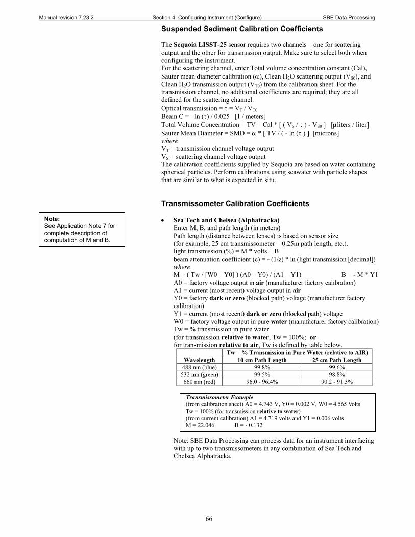
Manual revision 7.23.2 Section 4: Configuring Instrument (Configure) SBE Data Processing
66
Suspended Sediment Calibration Coefficients
The Sequoia LISST-25 sensor requires two channels – one for scattering output and the other for transmission output. Make sure to select both when configuring the instrument. For the scattering channel, enter Total volume concentration constant (Cal), Sauter mean diameter calibration (α), Clean H2O scattering output (VS0), and Clean H2O transmission output (VT0) from the calibration sheet. For the transmission channel, no additional coefficients are required; they are all defined for the scattering channel. Optical transmission = τ = VT / VT0 Beam C = - ln (τ) / 0.025 [1 / meters] Total Volume Concentration = TV = Cal * [ ( VS / τ ) - VS0 ] [µliters / liter] Sauter Mean Diameter = SMD = α * [ TV / ( - ln (τ ) ] [microns] where VT = transmission channel voltage output VS = scattering channel voltage output The calibration coefficients supplied by Sequoia are based on water containing spherical particles. Perform calibrations using seawater with particle shapes that are similar to what is expected in situ. Transmissometer Calibration Coefficients • Sea Tech and Chelsea (Alphatracka)
Enter M, B, and path length (in meters) Path length (distance between lenses) is based on sensor size (for example, 25 cm transmissometer = 0.25m path length, etc.). light transmission (%) = M * volts + B beam attenuation coefficient (c) = - (1/z) * ln (light transmission [decimal]) where M = ( Tw / [W0 – Y0] ) (A0 – Y0) / (A1 – Y1) B = - M * Y1 A0 = factory voltage output in air (manufacturer factory calibration) A1 = current (most recent) voltage output in air Y0 = factory dark or zero (blocked path) voltage (manufacturer factory calibration) Y1 = current (most recent) dark or zero (blocked path) voltage W0 = factory voltage output in pure water (manufacturer factory calibration) Tw = % transmission in pure water (for transmission relative to water, Tw = 100%; or for transmission relative to air, Tw is defined by table below.
Tw = % Transmission in Pure Water (relative to AIR) Wavelength 10 cm Path Length 25 cm Path Length
488 nm (blue) 99.8% 99.6% 532 nm (green) 99.5% 98.8% 660 nm (red) 96.0 - 96.4% 90.2 - 91.3%
Transmissometer Example (from calibration sheet) A0 = 4.743 V, Y0 = 0.002 V, W0 = 4.565 Volts Tw = 100% (for transmission relative to water) (from current calibration) A1 = 4.719 volts and Y1 = 0.006 volts M = 22.046 B = - 0.132
Note: SBE Data Processing can process data for an instrument interfacing with up to two transmissometers in any combination of Sea Tech and Chelsea Alphatracka,
Note: See Application Note 7 for complete description of computation of M and B.
Manual revision 7.23.2 Section 4: Configuring Instrument (Configure) SBE Data Processing
67
• WET Labs AC3 This sensor requires two channels - one for fluorometer voltage (listed under fluorometers in the dialog box) and the other for transmissometer voltage (listed under transmissometers). Make sure to select both when configuring the instrument. Enter Ch2o, Vh2o, VDark, and X from calibration sheet. Beam attenuation = {[log (Vh2o - VDark) - log (V - VDark)] /X} + Ch2o Beam transmission (%) = exp ( -beam attenuation * X) * 100
• WET Labs C-Star
Enter M, B, and path length (in meters) Path length (distance between lenses) is based on sensor size (for example, 25 cm transmissometer = 0.25m path length, etc.). light transmission (%) = M * volts + B beam attenuation coefficient (c) = - (1/z) * ln (light transmission [decimal]) where M = ( Tw / [W0 – Y0] ) (A0 – Y0) / (A1 – Y1) B = - M * Y1 A0 = Vair = factory voltage output in air (manufacturer factory calibration) A1 = current (most recent) voltage output in air Y0 = Vd = factory dark or zero (blocked path) voltage (manufacturer factory calibration) Y1 = current (most recent) dark or zero (blocked path) voltage W0 = Vref = factory voltage output in pure water (manufacturer factory calibration) Tw = % transmission in pure water (for transmission relative to water, Tw = 100%; or for transmission relative to air, Tw is defined by table below.
Tw = % Transmission in Pure Water (relative to AIR) Wavelength 10 cm Path Length 25 cm Path Length
488 nm (blue) 99.8% 99.6% 532 nm (green) 99.5% 98.8% 660 nm (red) 96.0 - 96.4% 90.2 - 91.3%
Transmissometer Example (from calibration sheet) Vair = 4.743 V, Vd = 0.002 V, Vref = 4.565 V Tw = 100% (for transmission relative to water) (from current calibration) A1 = 4.719 volts and Y1 = 0.006 volts M = 22.046 B = - 0.132
Note: SBE Data Processing can process data for an instrument interfacing with up to six WET Labs C-Stars.
Manual revision 7.23.2 Section 4: Configuring Instrument (Configure) SBE Data Processing
68
User Polynomial (for user-defined sensor) Calibration Coefficients The user polynomial allows you to define an equation to relate the sensor output voltage to calculated engineering units, if your sensor is not pre-defined in Sea-Bird software. Enter a0, a1, a2, and a3. Val = a0 + (a1 * V) + (a2 * V2) + (a3 * V3) where: V = voltage from sensor a0, a1, a2, and a3 = user-defined sensor polynomial coefficients If desired, enter the sensor name. This name will appear in the data file header. Note: SBE Data Processing can process data for an instrument interfacing with up to three sensors defined with user polynomials. Example A manufacturer defines the output of their sensor as: NTU = (Vsample – Vblank) * scale factor Set this equal to user polynomial equation and calculate a0, a1, a2, and a3. (Vsample – Vblank) * scale factor = a0 + (a1 * V) + (a2 * V2) + (a3 * V3) Expanding left side of equation and using consistent notation (Vsample = V): scale factor * V – scale factor * Vblank = a0 + (a1 * V) + (a2 * V2) + (a3 * V3) Left side of equation has no V2 or V3 terms, so a2 and a3 are 0; rearranging: (– scale factor * Vblank) + (scale factor * V) = a0 + (a1 * V) a0 = – scale factor * Vblank a1 = scale factor a2 = a3 = 0 Zaps Calibration Coefficients Enter M and B from calibration sheet. z = (M * volts) + B [nmoles]
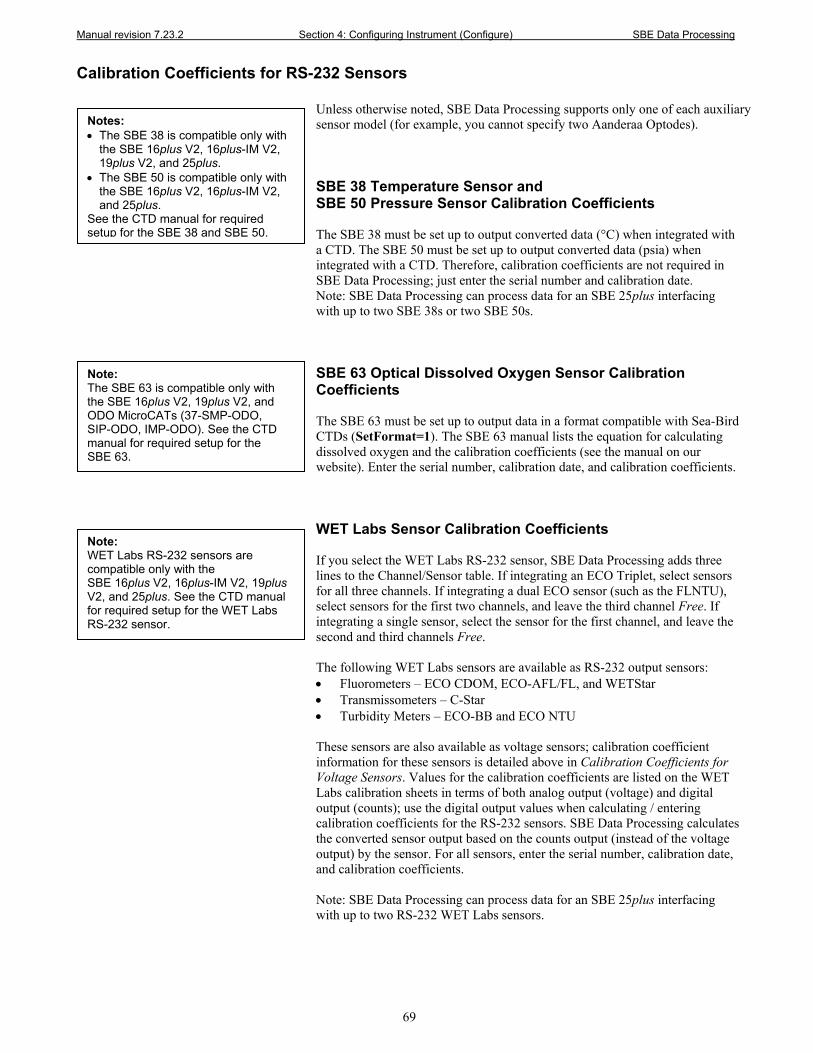
Manual revision 7.23.2 Section 4: Configuring Instrument (Configure) SBE Data Processing
69
Calibration Coefficients for RS-232 Sensors Unless otherwise noted, SBE Data Processing supports only one of each auxiliary sensor model (for example, you cannot specify two Aanderaa Optodes). SBE 38 Temperature Sensor and SBE 50 Pressure Sensor Calibration Coefficients The SBE 38 must be set up to output converted data (°C) when integrated with a CTD. The SBE 50 must be set up to output converted data (psia) when integrated with a CTD. Therefore, calibration coefficients are not required in SBE Data Processing; just enter the serial number and calibration date. Note: SBE Data Processing can process data for an SBE 25plus interfacing with up to two SBE 38s or two SBE 50s. SBE 63 Optical Dissolved Oxygen Sensor Calibration Coefficients The SBE 63 must be set up to output data in a format compatible with Sea-Bird CTDs (SetFormat=1). The SBE 63 manual lists the equation for calculating dissolved oxygen and the calibration coefficients (see the manual on our website). Enter the serial number, calibration date, and calibration coefficients. WET Labs Sensor Calibration Coefficients If you select the WET Labs RS-232 sensor, SBE Data Processing adds three lines to the Channel/Sensor table. If integrating an ECO Triplet, select sensors for all three channels. If integrating a dual ECO sensor (such as the FLNTU), select sensors for the first two channels, and leave the third channel Free. If integrating a single sensor, select the sensor for the first channel, and leave the second and third channels Free. The following WET Labs sensors are available as RS-232 output sensors: • Fluorometers – ECO CDOM, ECO-AFL/FL, and WETStar • Transmissometers – C-Star • Turbidity Meters – ECO-BB and ECO NTU These sensors are also available as voltage sensors; calibration coefficient information for these sensors is detailed above in Calibration Coefficients for Voltage Sensors. Values for the calibration coefficients are listed on the WET Labs calibration sheets in terms of both analog output (voltage) and digital output (counts); use the digital output values when calculating / entering calibration coefficients for the RS-232 sensors. SBE Data Processing calculates the converted sensor output based on the counts output (instead of the voltage output) by the sensor. For all sensors, enter the serial number, calibration date, and calibration coefficients. Note: SBE Data Processing can process data for an SBE 25plus interfacing with up to two RS-232 WET Labs sensors.
Notes: • The SBE 38 is compatible only with
the SBE 16plus V2, 16plus-IM V2, 19plus V2, and 25plus.
• The SBE 50 is compatible only with the SBE 16plus V2, 16plus-IM V2, and 25plus.
See the CTD manual for required setup for the SBE 38 and SBE 50.
Note: WET Labs RS-232 sensors are compatible only with the SBE 16plus V2, 16plus-IM V2, 19plus V2, and 25plus. See the CTD manual for required setup for the WET Labs RS-232 sensor.
Note: The SBE 63 is compatible only with the SBE 16plus V2, 19plus V2, and ODO MicroCATs (37-SMP-ODO, SIP-ODO, IMP-ODO). See the CTD manual for required setup for the SBE 63.
Manual revision 7.23.2 Section 4: Configuring Instrument (Configure) SBE Data Processing
70
GTD Calibration Coefficients The GTD must be set up to output converted data (millibars) when integrated with a CTD. Therefore, calibration coefficients are not required in SBE Data Processing; just enter the serial number and calibration date. Aanderaa Oxygen Optode Calibration Coefficients Enter the serial number, calibration date, and information required for salinity and depth corrections. The internal salinity must match the value you programmed into the Optode (the value is ignored if you do not enable the Salinity correction). If you enable Salinity correction, SBE Data Processing corrects the oxygen output from the Optode based on the actual salinity (calculated from the CTD data). If you enable Depth correction, SBE Data Processing corrects the oxygen output from the Optode based on the depth (calculated from the CTD data).
Notes: • The Optode is compatible only with
the SBE 16plus V2, 16plus-IM V2, and 19plus V2. See the CTD manual for required setup for the Optode.
• See Calibration Coefficients for Voltage Sensors above for voltage-output Oxygen sensors, including the SBE 43.
Notes: • The GTD is compatible only with the
SBE 16plus V2, 16plus-IM V2, and 19plus V2. See the CTD manual for required setup for the GTD.
• SBE Data Processing supports single or dual GTDs.
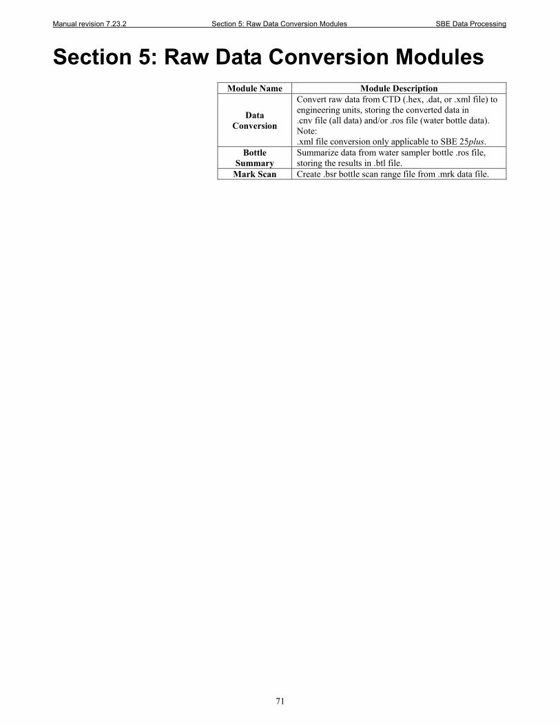
Manual revision 7.23.2 Section 5: Raw Data Conversion Modules SBE Data Processing
71
Section 5: Raw Data Conversion Modules
Module Name Module Description
Data Conversion
Convert raw data from CTD (.hex, .dat, or .xml file) to engineering units, storing the converted data in .cnv file (all data) and/or .ros file (water bottle data). Note: .xml file conversion only applicable to SBE 25plus.
Bottle Summary
Summarize data from water sampler bottle .ros file, storing the results in .btl file.
Mark Scan Create .bsr bottle scan range file from .mrk data file.
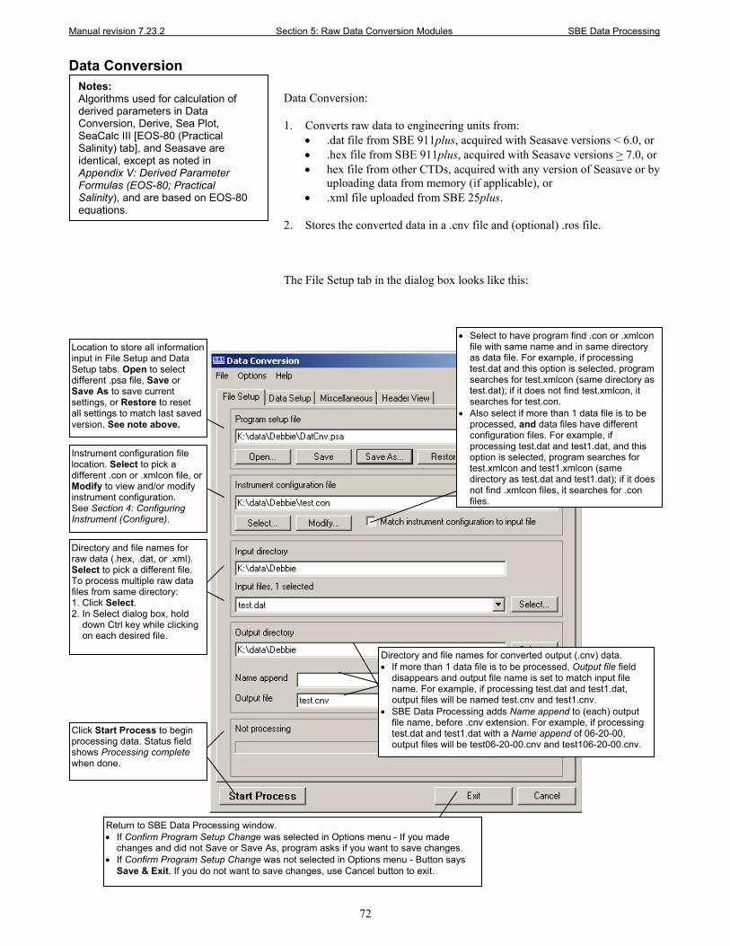
Manual revision 7.23.2 Section 5: Raw Data Conversion Modules SBE Data Processing
72
Data Conversion Data Conversion: 1. Converts raw data to engineering units from:
• .dat file from SBE 911plus, acquired with Seasave versions < 6.0, or • .hex file from SBE 911plus, acquired with Seasave versions > 7.0, or • hex file from other CTDs, acquired with any version of Seasave or by
uploading data from memory (if applicable), or • .xml file uploaded from SBE 25plus.
2. Stores the converted data in a .cnv file and (optional) .ros file. The File Setup tab in the dialog box looks like this:
Notes: Algorithms used for calculation of derived parameters in Data Conversion, Derive, Sea Plot, SeaCalc III [EOS-80 (Practical Salinity) tab], and Seasave are identical, except as noted in Appendix V: Derived Parameter Formulas (EOS-80; Practical Salinity), and are based on EOS-80 equations.
Location to store all information input in File Setup and Data Setup tabs. Open to select different .psa file, Save or Save As to save current settings, or Restore to reset all settings to match last saved version. See note above.
Instrument configuration file location. Select to pick a different .con or .xmlcon file, or Modify to view and/or modify instrument configuration. See Section 4: Configuring Instrument (Configure).
Directory and file names for raw data (.hex, .dat, or .xml). Select to pick a different file. To process multiple raw data files from same directory: 1. Click Select. 2. In Select dialog box, hold
down Ctrl key while clicking on each desired file.
Directory and file names for converted output (.cnv) data. • If more than 1 data file is to be processed, Output file field
disappears and output file name is set to match input file name. For example, if processing test.dat and test1.dat, output files will be named test.cnv and test1.cnv.
• SBE Data Processing adds Name append to (each) output file name, before .cnv extension. For example, if processing test.dat and test1.dat with a Name append of 06-20-00, output files will be test06-20-00.cnv and test106-20-00.cnv.
Click Start Process to begin processing data. Status field shows Processing complete when done.
Return to SBE Data Processing window. • If Confirm Program Setup Change was selected in Options menu - If you made
changes and did not Save or Save As, program asks if you want to save changes. • If Confirm Program Setup Change was not selected in Options menu - Button says
Save & Exit. If you do not want to save changes, use Cancel button to exit.
• Select to have program find .con or .xmlcon file with same name and in same directory as data file. For example, if processing test.dat and this option is selected, program searches for test.xmlcon (same directory as test.dat); if it does not find test.xmlcon, it searches for test.con.
• Also select if more than 1 data file is to be processed, and data files have different configuration files. For example, if processing test.dat and test1.dat, and this option is selected, program searches for test.xmlcon and test1.xmlcon (same directory as test.dat and test1.dat); if it does not find .xmlcon files, it searches for .con files.
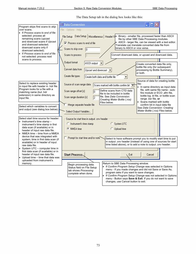
Manual revision 7.23.2 Section 5: Raw Data Conversion Modules SBE Data Processing
73
The Data Setup tab in the dialog box looks like this:
Program skips first scans to skip over scans. • If Process scans to end of file
selected: process all remaining scans (upcast and downcast scans if Upcast and downcast selected; downcast scans only if downcast selected).
• If Process scans to end of file not selected: process next scans to process.
Define scans from CTD data file to be included in bottle file. See Data Conversion: Creating Water Bottle (.ros) Files below.
Begin processing data. Status field on File Setup tab shows Processing complete when done.
Return to SBE Data Processing window. • If Confirm Program Setup Change was selected in Options
menu - If you made changes and did not Save or Save As, program asks if you want to save changes.
• If Confirm Program Setup Change was not selected in Options menu - Button says Save & Exit. If you do not want to save changes, use Cancel button to exit.
Create converted data file only, bottle file only (for subsequent processing by Bottle Summary), or both.
Convert downcast data, or upcast and downcast data.
• Binary - smaller file, processed faster than ASCII file by other SBE Data Processing modules.
• ASCII - larger file, can be viewed with a text editor. Translate can translate converted data file from binary to ASCII or vice versa.
Source of data for creating bottle file: • In same directory as input data
file, with same file name - auto fire module or ECO .afm file, bottle log .bl file, or bottle scan range .bsr file, or
• Scans marked with bottle confirm bit in input data file
See Data Conversion: Creating Water Bottle (.ros) Files below.
Select to have software prompt you to modify start time to put in output .cnv header (instead of using one of sources for start time listed above), or to add a note to output .cnv header.
Select to replace existing header in input file with header in .hdr file. Program looks for a file with a matching name (but .hdr extension) in same directory as input file.
Select which variables to convert and output (see dialog box below).
Select start time source for header: • Instrument’s time stamp –
instrument’s time stamp in first data scan (if available) or in header of input raw data file.
• NMEA time – time from a NMEA device that was integrated with system; time in first data scan (if available) or in header of input raw data file.
• System UTC – computer time in first data scan (if available) or in header of input raw data file.
• Upload time – time that data was uploaded from instrument’s memory.
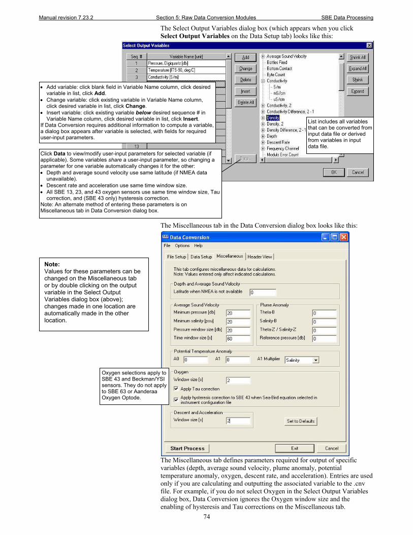
Manual revision 7.23.2 Section 5: Raw Data Conversion Modules SBE Data Processing
74
The Select Output Variables dialog box (which appears when you click Select Output Variables on the Data Setup tab) looks like this:
The Miscellaneous tab in the Data Conversion dialog box looks like this:
The Miscellaneous tab defines parameters required for output of specific variables (depth, average sound velocity, plume anomaly, potential temperature anomaly, oxygen, descent rate, and acceleration). Entries are used only if you are calculating and outputting the associated variable to the .cnv file. For example, if you do not select Oxygen in the Select Output Variables dialog box, Data Conversion ignores the Oxygen window size and the enabling of hysteresis and Tau corrections on the Miscellaneous tab.
• Add variable: click blank field in Variable Name column, click desired variable in list, click Add.
• Change variable: click existing variable in Variable Name column, click desired variable in list, click Change.
• Insert variable: click existing variable below desired sequence # in Variable Name column, click desired variable in list, click Insert.
If Data Conversion requires additional information to compute a variable, a dialog box appears after variable is selected, with fields for required user-input parameters.
List includes all variables that can be converted from input data file or derived from variables in input data file.
Click Data to view/modify user-input parameters for selected variable (if applicable). Some variables share a user-input parameter, so changing a parameter for one variable automatically changes it for the other: • Depth and average sound velocity use same latitude (if NMEA data
unavailable). • Descent rate and acceleration use same time window size. • All SBE 13, 23, and 43 oxygen sensors use same time window size, Tau
correction, and (SBE 43 only) hysteresis correction. Note: An alternate method of entering these parameters is on Miscellaneous tab in Data Conversion dialog box.
Note: Values for these parameters can be changed on the Miscellaneous tab or by double clicking on the output variable in the Select Output Variables dialog box (above); changes made in one location are automatically made in the other location.
Oxygen selections apply to SBE 43 and Beckman/YSI sensors. They do not apply to SBE 63 or Aanderaa Oxygen Optode.
Manual revision 7.23.2 Section 5: Raw Data Conversion Modules SBE Data Processing
75
Data Conversion: Creating Water Bottle (.ros) Files
A .ros water bottle file contains: • data for each scan associated with a bottle firing, and • data for user-selected range of scans before and after each bottle firing Scan range data for creation of a water bottle file can come from: • Scans marked with bottle confirm bit in input data file - if used
- SBE 9plus with an SBE 11plus Deck Unit and G.O. 1015 Rosette, or - SBE 9plus with an SBE 17plus Searam and SBE 32 Carousel Water Sampler. For these systems, the bottle confirm bit in the input (.hex or .dat) data file is set for all scans within a 1.5-second duration after a bottle firing confirmation is received from the water sampler.
• Bottle log (.bl) file - if used Seasave to interface with - SBE 9plus with SBE 11plus Deck Unit and G.O. 1016 Rosette or SBE 32 Carousel Water Sampler, or - SBE 19, 19plus, 19plus V2, 25, or 49 with SBE 33 Deck Unit and SBE 32 Carousel Water Sampler, or - SBE 19, 19plus, 19plus V2, 25, or 49 with SBE 33 Deck Unit and SBE 55 ECO Water Sampler. For these systems, Seasave creates the .bl file. Each time a bottle fire confirmation is received, the bottle sequence number, position, date, time, and beginning and ending scan numbers (1.5-second duration for each bottle) are written to the .bl file.
• Auto Fire Module or ECO (.afm) file - if used - Carousel Auto Fire Module (AFM) with SBE 19, 19plus, 19plus V2, 25, or 50 and SBE 32 Carousel Water Sampler, or - SBE 19, 19plus, 19plus V2, 25, or 50 and SBE 55 ECO Water Sampler (autonomous operation). For these systems, the .afm file contains five scans of data recorded by the AFM or SBE 55 ECO Water Sampler for each bottle firing.
• Bottle scan range (.bsr) file - if used Mark Scan feature in Seasave during data acquisition to create a .mrk file; use Mark Scan to convert the .mrk file to a .bsr file before running Data Conversion. The format for the .bsr file is: beginning scan # for bottle #1, ending scan # for bottle #1 … beginning scan # for last bottle, ending scan # for last bottle Example: test.bsr contains - 1000, 1020 2000, 2020 4000, 4020 The .ros file created using test.bsr would contain scans 1000 - 1020 for bottle #1, 2000 - 2020 for bottle #2, and 4000 - 4020 for bottle #3.
The amount of data written to the .ros file is based on: • Scan range offset - determines the first scan output to the .ros file for
each bottle, relative to the first scan with a confirmation bit set or written to a .afm, .bsr, or .bl file.
• Scan range duration - determines the number of scans output to the .ros file for each bottle.
Example: A bottle confirmation for an SBE 911plus is received at scan 10,000 (scan 10,000 and subsequent scans for 1.5 seconds have confirmation bit set). In Data Conversion, Scan range offset is set to -2 seconds, and Scan range duration is set to 5 seconds. If the scan rate is 24 scans/second, 10,000 - 2 second offset (24 scans/second) = 9,952 9,952 + 5 second duration (24 scans/second) = 10,072 Therefore, scans 9,952 through 10,072 will be written to the .ros file.
Notes: • You may have more than one
source of scan range data available. For example, if Seasave is used with an SBE 911plus and SBE 32 Carousel Water Sampler, a bottle log (.bl) file is created. Additionally, if you used the Mark Scan feature in Seasave, a .mrk file is created.
• If scan range data is defined by a .afm file, Data Conversion creates a .bl file (same name as input data file, with .bl extension). The .bl file is used when processing the water bottle data in Bottle Summary.
• You can create a .bsr file in a text editor if scan range data is not available in any of these forms.
Manual revision 7.23.2 Section 5: Raw Data Conversion Modules SBE Data Processing
76
Data Conversion: Notes and General Information Data Conversion was written to accommodate most sensors that have been installed on Sea-Bird products. See the configuration page at the beginning of your instrument manual for the sensors that were installed on your system.
• If you plan to process the data with other modules, select only the primary variables to be converted, and then use Derive to compute derived parameters such as salinity, density, sound velocity, and oxygen.
• If desired, you can select the same variable multiple times for the output .cnv file. If you do, data processing operations on that variable in other modules will use the last occurrence of the variable in the file. Example: Select Primary Conductivity, Primary Temperature, Pressure, and Primary Conductivity (again) for output variables (columns 1, 2, 3, and 4 respectively). Then, if you run Cell Thermal Mass, it will correct the conductivity in column 4 only, leaving column 1 uncorrected; you could plot the corrected and uncorrected conductivity to see the changes. If you then run Derive to calculate salinity, it will use the corrected conductivity in column 4 in the salinity calculation.
• If you will use Derive to compute: Salinity, density, or other parameters that depend on salinity -
include pressure, temperature, and conductivity in the output file. For a moored instrument without optional pressure sensor (SBE 16, 16plus, 16plus-IM, 16plus V2, or 16plus-IM V2), if you select pressure as an output variable, Data Conversion inserts a column with the moored pressure (entered in the configuration file Data dialog) in the output .cnv file. For a thermosalinograph (SBE 21 or 45), if you select pressure as an output variable, Data Conversion inserts a column of 0’s for the pressure in the output .cnv file. The pressure column is needed for Derive to calculate salinity, density, etc.
Oxygen - include in the output file (along with pressure, temperature, and conductivity) For SBE 13 or 23 - oxygen current and oxygen temperature For SBE 43 - oxygen value
• If you will use Bin Average: With depth bins - include depth in the output file With pressure bins - include pressure in the output file
• Pressure temperature is computed using a backward-looking, 30-second running average, to prevent bit transitions in pressure temperature from causing small jumps in computed pressure. Because the heavily insulated pressure sensor has a thermal time constant on the order of one hour, the 30-second average does not significantly alter the computed pressure temperature.
• Oxygen, descent rate, and acceleration computed by Seasave and Data Conversion are somewhat different from values computed by Derive, because the algorithms calculate the derivative of the signal (oxygen signal for oxygen, pressure signal for descent rate and acceleration) with respect to time, using a linear regression to determine the slope. Seasave and Data Conversion compute the derivative looking backward in time, since they share common code and Seasave cannot use future values while acquiring data in real time. Derive uses a centered window (equal number of points before and after the scan; time window size is user input) to obtain a better estimate of the derivative. Use Seasave and Data Conversion to obtain a quick look at oxygen, descent rate, and acceleration; use Derive to obtain the most accurate values.
• For an SBE 21 or 45 with a remote temperature sensor, Seasave, Data Conversion, Derive, and Derive TEOS-10 all use the remote temperature data when calculating density and sound velocity.
Note: If you choose to compute derived parameters in Data Conversion, note that the algorithms are the same as used in Derive (with the exception of the oxygen, descent rate, and acceleration calculations); see Appendix V: Derived Parameter Formulas for algorithms for derived variables.
Manual revision 7.23.2 Section 5: Raw Data Conversion Modules SBE Data Processing
77
Data Conversion has the following /x parameters when run from the Command Line Options dialog box, from the command line, or with batch file processing:
/x Parameter Description /xdatcnv:skipN N = number of scans to skip.
/xdatcnv:pump For SBE 911plus, do not output scans if pump status = off.
/xdatcnv:nomatch Disable matching of header information to .con or .xmlcon configuration file - program continues to run even if there is a discrepancy in header information.
See Appendix I: Command Line Options, Command Line Operation, and Batch File Processing for details on using parameters. Data Conversion adds the following to the data file header for a .cnv converted data file:
Label Description
Nquan
Number of columns (fields) of converted data. Note: Data Conversion automatically adds 1 field to number selected by user (i.e., if user selects 3 variables to convert, then nquan=4). This added field, initially set to 0, is used by Loop Edit to mark bad scans.
Nvalues Number of scans converted.
Units Specified (indicates units are specified separately for each variable).
Name n Sensor (and units) associated with data in column n. Span n Span (highest - lowest value) of data in column n. Interval Scan rate (seconds).
Start_time Data start time.
Bad_flag For information only; value that Loop Edit and Wild Edit will use to mark bad scans and bad data values.
Sensors Sensor description, serial number, and calibration date and coefficients, all in XML format.
Datcnv_date Date and time that module was run. Also shows how many columns of data output (not including flag column).
Datcnv_in Input .hex (or .dat) data file and .con or .xmlcon configuration file.
Datcnv_skipover Number of scans to skip over in processing. Datcnv_ox_
hysteresis_correction Whether hysteresis correction was performed on oxygen data.
Datcnv_ox_tau_ correction Whether tau correction was performed on oxygen data.
File type Selected output file type - ASCII or binary. Data Conversion adds the following to the data file header for a .ros water bottle file:
Label Description
Nquan
Number of columns (fields) of converted data. Note: Data Conversion automatically adds 1 field to number selected by user (i.e., if user selects 3 variables to convert, then nquan=4). This added field, initially set to 0, is used by Loop Edit to mark bad scans.
Nvalues Number of scans converted.
Units Specified (indicates units are specified separately for each variable).
Name n Sensor (and units) associated with data in column n. Interval Scan rate (seconds).
Start_time Data start time.
Sensors Sensor description, serial number, and calibration date and coefficients, all in XML format.
Datcnv_date Date and time that module was run.
Datcnv_in Input .hex (or .dat) data file and .con or .xmlcon configuration file.
Datcnv_bottle_ scan_range_source
Source of data for creating bottle file, and scan range offset and duration.
Datcnv_scans_ per_bottle
Number of data scans/bottle in .ros file; based on scan range offset and duration, and CTD sampling rate
Notes: • Each SBE Data Processing
module that modifies a .cnv file adds information to the header and updates nquan, nvalues, name n, span n, interval, and file_type, as applicable.
• Calibration coefficients were added to the file header for a .cnv file and for a .ros water bottle file in SBE Data Processing version 7.19.
Manual revision 7.23.2 Section 5: Raw Data Conversion Modules SBE Data Processing
78
Bottle Summary
Bottle Summary reads a .ros file created by Data Conversion and writes a bottle data summary to a .btl file. The .ros file must contain (as a minimum) temperature, pressure, and conductivity (or salinity). The output .btl file includes: • Bottle position, optional bottle serial number, and date/time • User-selected derived variables - computed for each bottle from mean
values of input variables (temperature, pressure, conductivity, etc.) • User-selected averaged variables - computed for each bottle from
input variables The maximum number of scans processed per bottle is 1440. In addition to the .ros input file: • If a .bl file (same name as input data file, with .bl extension) is found in
the input file directory, Bottle Summary uses bottle position data from the .bl file. The bottle position data defines the bottle firing sequence - the .bl file contains the bottle firing sequence number, bottle position, date and time, and beginning and ending scan number for each bottle.
• If a .sn file (same name as input data file, with .sn extension) is found in
the input file directory, bottle serial numbers are inserted between the bottle position and date/time columns in the .btl file output. The format for the .sn file is: Bottle position, serial number (with a comma separating the two fields)
Note: You can create a .sn file in a text editor.
Note: Bottle Summary was previously called Rosette Summary.
Note: A .bl file is created by: • Seasave, during real-time data
acquisition, or • Data Conversion, if the source of
scan rage data was a .afm file.
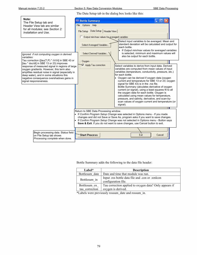
Manual revision 7.23.2 Section 5: Raw Data Conversion Modules SBE Data Processing
79
The Data Setup tab in the dialog box looks like this:
Bottle Summary adds the following to the data file header:
Label* Description Bottlesum_date Date and time that module was run.
Bottlesum_in Input .ros bottle data file and .con or .xmlcon configuration file.
Bottlesum_ox_ tau_correction
Tau correction applied to oxygen data? Only appears if oxygen is derived.
*Labels were previously rossum_date and rossum_in.
Note: The File Setup tab and Header View tab are similar for all modules; see Section 2: Installation and Use.
Select input variables to be averaged. Mean and standard deviation will be calculated and output for each bottle. • If Output min/max values for averaged variables
is selected, minimum and maximum values will also be output for each bottle.
Return to SBE Data Processing window. • If Confirm Program Setup Change was selected in Options menu - If you made
changes and did not Save or Save As, program asks if you want to save changes. • If Confirm Program Setup Change was not selected in Options menu - Button says
Save & Exit. If you do not want to save changes, use Cancel button to exit.
Begin processing data. Status field on File Setup tab shows Processing complete when done.
Select variables to derive from input data. Derived variables are computed from mean values of input variables (temperature, conductivity, pressure, etc.) for each bottle. • Oxygen can be derived if oxygen data (oxygen
current and temperature for SBE 13 or 23; oxygen signal for SBE 43) is in the .ros file. Bottle Summary calculates derivative of oxygen current (or signal), using a least squares fit to all the oxygen data for each bottle. Oxygen is calculated using mean values for temperature, pressure, and salinity, derivative, and scan-by-scan values of oxygen current and temperature (or signal).
Ignored if not computing oxygen in derived variables: Tau correction ([tau(T,P) * δV/δt] in SBE 43 or [tau * doc/dt] in SBE 13 or 23) improves response of measured signal in regions of large oxygen gradients. However, this term also amplifies residual noise in signal (especially in deep water), and in some situations this negative consequence overshadows gains in signal responsiveness.
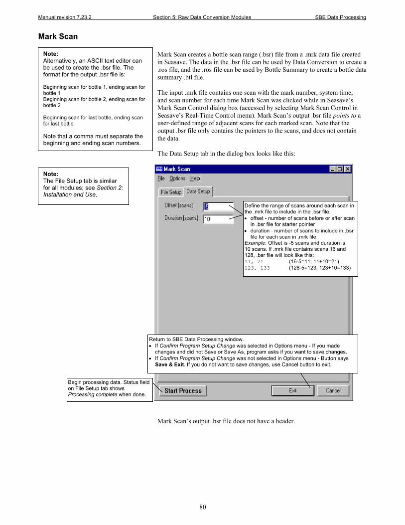
Manual revision 7.23.2 Section 5: Raw Data Conversion Modules SBE Data Processing
80
Mark Scan Mark Scan creates a bottle scan range (.bsr) file from a .mrk data file created in Seasave. The data in the .bsr file can be used by Data Conversion to create a .ros file, and the .ros file can be used by Bottle Summary to create a bottle data summary .btl file. The input .mrk file contains one scan with the mark number, system time, and scan number for each time Mark Scan was clicked while in Seasave’s Mark Scan Control dialog box (accessed by selecting Mark Scan Control in Seasave’s Real-Time Control menu). Mark Scan’s output .bsr file points to a user-defined range of adjacent scans for each marked scan. Note that the output .bsr file only contains the pointers to the scans, and does not contain the data. The Data Setup tab in the dialog box looks like this:
Mark Scan’s output .bsr file does not have a header.
Note: Alternatively, an ASCII text editor can be used to create the .bsr file. The format for the output .bsr file is: Beginning scan for bottle 1, ending scan for bottle 1 Beginning scan for bottle 2, ending scan for bottle 2 . Beginning scan for last bottle, ending scan for last bottle Note that a comma must separate the beginning and ending scan numbers.
Define the range of scans around each scan in the .mrk file to include in the .bsr file. • offset - number of scans before or after scan
in .bsr file for starter pointer • duration - number of scans to include in .bsr
file for each scan in .mrk file Example: Offset is -5 scans and duration is 10 scans. If .mrk file contains scans 16 and 128, .bsr file will look like this: 11, 21 (16-5=11; 11+10=21) 123, 133 (128-5=123; 123+10=133)
Return to SBE Data Processing window. • If Confirm Program Setup Change was selected in Options menu - If you made
changes and did not Save or Save As, program asks if you want to save changes. • If Confirm Program Setup Change was not selected in Options menu - Button says
Save & Exit. If you do not want to save changes, use Cancel button to exit.
Begin processing data. Status field on File Setup tab shows Processing complete when done.
Note: The File Setup tab is similar for all modules; see Section 2: Installation and Use.
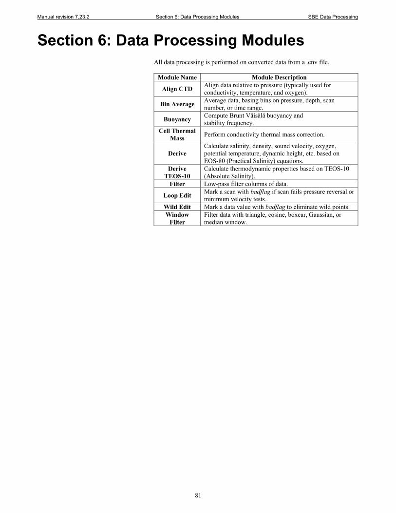
Manual revision 7.23.2 Section 6: Data Processing Modules SBE Data Processing
81
Section 6: Data Processing Modules
All data processing is performed on converted data from a .cnv file.
Module Name Module Description
Align CTD Align data relative to pressure (typically used for conductivity, temperature, and oxygen).
Bin Average Average data, basing bins on pressure, depth, scan number, or time range.
Buoyancy Compute Brunt Väisälä buoyancy and stability frequency.
Cell Thermal Mass Perform conductivity thermal mass correction.
Derive Calculate salinity, density, sound velocity, oxygen, potential temperature, dynamic height, etc. based on EOS-80 (Practical Salinity) equations.
Derive TEOS-10
Calculate thermodynamic properties based on TEOS-10 (Absolute Salinity).
Filter Low-pass filter columns of data.
Loop Edit Mark a scan with badflag if scan fails pressure reversal or minimum velocity tests.
Wild Edit Mark a data value with badflag to eliminate wild points. Window
Filter Filter data with triangle, cosine, boxcar, Gaussian, or median window.
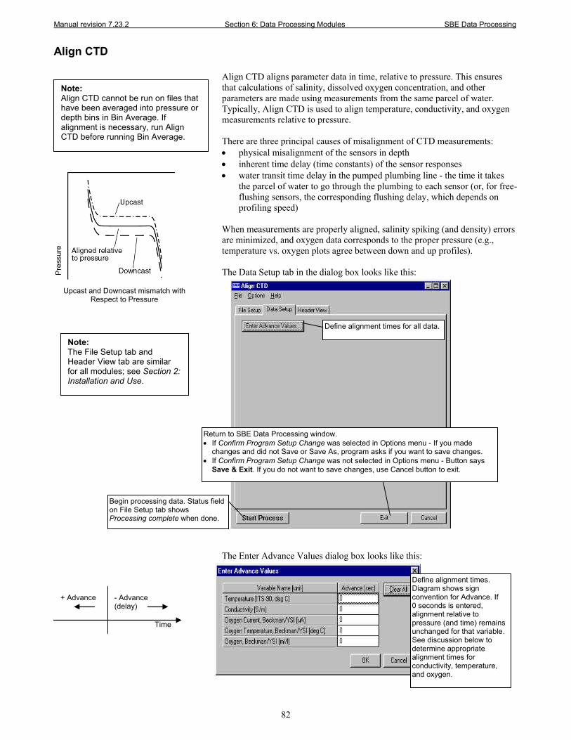
Manual revision 7.23.2 Section 6: Data Processing Modules SBE Data Processing
82
Align CTD Align CTD aligns parameter data in time, relative to pressure. This ensures that calculations of salinity, dissolved oxygen concentration, and other parameters are made using measurements from the same parcel of water. Typically, Align CTD is used to align temperature, conductivity, and oxygen measurements relative to pressure. There are three principal causes of misalignment of CTD measurements: • physical misalignment of the sensors in depth • inherent time delay (time constants) of the sensor responses • water transit time delay in the pumped plumbing line - the time it takes
the parcel of water to go through the plumbing to each sensor (or, for free-flushing sensors, the corresponding flushing delay, which depends on profiling speed)
When measurements are properly aligned, salinity spiking (and density) errors are minimized, and oxygen data corresponds to the proper pressure (e.g., temperature vs. oxygen plots agree between down and up profiles). The Data Setup tab in the dialog box looks like this:
The Enter Advance Values dialog box looks like this:
Define alignment times. Diagram shows sign convention for Advance. If 0 seconds is entered, alignment relative to pressure (and time) remains unchanged for that variable. See discussion below to determine appropriate alignment times for conductivity, temperature, and oxygen.
Note: Align CTD cannot be run on files that have been averaged into pressure or depth bins in Bin Average. If alignment is necessary, run Align CTD before running Bin Average.
- Advance (delay)
+ Advance
Time
Upcast and Downcast mismatch with Respect to Pressure
Define alignment times for all data.
Return to SBE Data Processing window. • If Confirm Program Setup Change was selected in Options menu - If you made
changes and did not Save or Save As, program asks if you want to save changes. • If Confirm Program Setup Change was not selected in Options menu - Button says
Save & Exit. If you do not want to save changes, use Cancel button to exit.
Begin processing data. Status field on File Setup tab shows Processing complete when done.
Note: The File Setup tab and Header View tab are similar for all modules; see Section 2: Installation and Use.
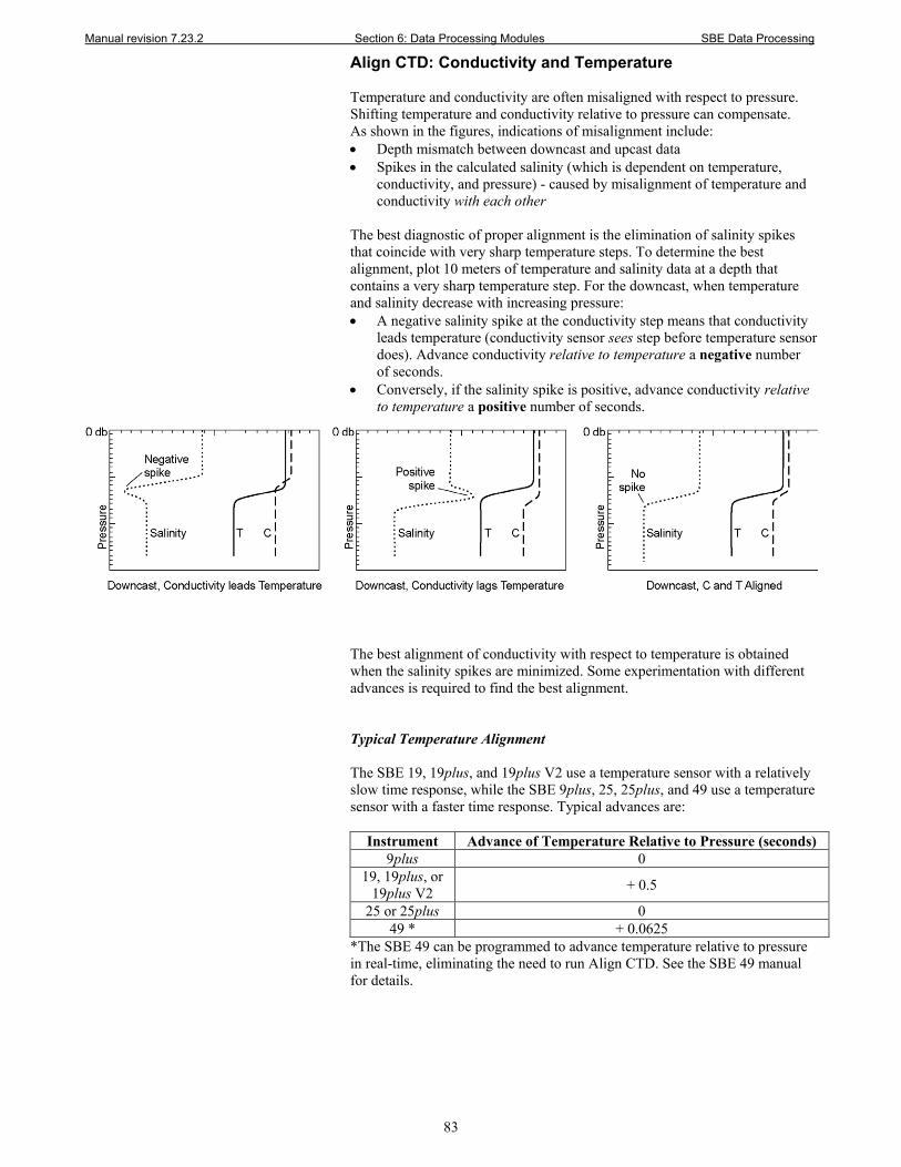
Manual revision 7.23.2 Section 6: Data Processing Modules SBE Data Processing
83
Align CTD: Conductivity and Temperature Temperature and conductivity are often misaligned with respect to pressure. Shifting temperature and conductivity relative to pressure can compensate. As shown in the figures, indications of misalignment include: • Depth mismatch between downcast and upcast data • Spikes in the calculated salinity (which is dependent on temperature,
conductivity, and pressure) - caused by misalignment of temperature and conductivity with each other
The best diagnostic of proper alignment is the elimination of salinity spikes that coincide with very sharp temperature steps. To determine the best alignment, plot 10 meters of temperature and salinity data at a depth that contains a very sharp temperature step. For the downcast, when temperature and salinity decrease with increasing pressure: • A negative salinity spike at the conductivity step means that conductivity
leads temperature (conductivity sensor sees step before temperature sensor does). Advance conductivity relative to temperature a negative number of seconds.
• Conversely, if the salinity spike is positive, advance conductivity relative to temperature a positive number of seconds.
The best alignment of conductivity with respect to temperature is obtained when the salinity spikes are minimized. Some experimentation with different advances is required to find the best alignment. Typical Temperature Alignment The SBE 19, 19plus, and 19plus V2 use a temperature sensor with a relatively slow time response, while the SBE 9plus, 25, 25plus, and 49 use a temperature sensor with a faster time response. Typical advances are:
Instrument Advance of Temperature Relative to Pressure (seconds) 9plus 0
19, 19plus, or 19plus V2 + 0.5
25 or 25plus 0 49 * + 0.0625
*The SBE 49 can be programmed to advance temperature relative to pressure in real-time, eliminating the need to run Align CTD. See the SBE 49 manual for details.
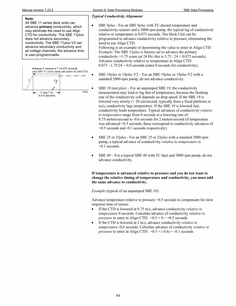
Manual revision 7.23.2 Section 6: Data Processing Modules SBE Data Processing
84
Typical Conductivity Alignment • SBE 9plus - For an SBE 9plus with TC-ducted temperature and
conductivity sensors and a 3000-rpm pump, the typical lag of conductivity relative to temperature is 0.073 seconds. The Deck Unit can be programmed to advance conductivity relative to pressure, eliminating the need to run Align CTD. Following is an example of determining the value to enter in Align CTD: Example: The SBE 11plus is factory-set to advance the primary conductivity +1.75 scans (at 24 Hz, this is 1.75 / 24 = 0.073 seconds). Advance conductivity relative to temperature in Align CTD: 0.073 - 1.75/24 = 0.0 seconds (enter 0 seconds for conductivity).
• SBE 19plus or 19plus V2 – For an SBE 19plus or 19plus V2 with a
standard 2000-rpm pump, do not advance conductivity.
• SBE 19 (not plus) – For an unpumped SBE 19, the conductivity measurement may lead or lag that of temperature, because the flushing rate of the conductivity cell depends on drop speed. If the SBE 19 is lowered very slowly (< 20 cm/second, typically from a fixed platform or ice), conductivity lags temperature. If the SBE 19 is lowered fast, conductivity leads temperature. Typical advances of conductivity relative to temperature range from 0 seconds at a lowering rate of 0.75 meters/second to -0.6 seconds for 2 meters/second (if temperature was advanced +0.5 seconds, these correspond to conductivity advances of +0.5 seconds and -0.1 seconds respectively).
• SBE 25 or 25plus - For an SBE 25 or 25plus with a standard 2000-rpm
pump, a typical advance of conductivity relative to temperature is +0.1 seconds.
• SBE 49 – For a typical SBE 49 with TC duct and 3000 rpm pump, do not
advance conductivity.
If temperature is advanced relative to pressure and you do not want to change the relative timing of temperature and conductivity, you must add the same advance to conductivity. Example (typical of an unpumped SBE 19): Advance temperature relative to pressure +0.5 seconds to compensate for slow response time of sensor. • If the CTD is lowered at 0.75 m/s, advance conductivity relative to
temperature 0 seconds. Calculate advance of conductivity relative to pressure to enter in Align CTD: +0.5 + 0 = +0.5 seconds
• If the CTD is lowered at 2 m/s, advance conductivity relative to temperature -0.6 seconds. Calculate advance of conductivity relative to pressure to enter in Align CTD: +0.5 + (-0.6) = -0.1 seconds
Note: All SBE 11 series deck units can advance primary conductivity, which may eliminate the need to use Align CTD for conductivity. The SBE 11plus does not advance secondary conductivity. The SBE 11plus V2 can advance secondary conductivity and all voltage channels; the advance time is user-programmable.
Manual revision 7.23.2 Section 6: Data Processing Modules SBE Data Processing
85
Align CTD: Oxygen
Oxygen data is also systematically delayed with respect to pressure. The two primary causes are the long time constant of the oxygen sensor (for the SBE 43, ranging from 2 seconds at 25 ºC to approximately 5 seconds at 0 ºC) and an additional delay from the transit time of water in the pumped plumbing line. As with temperature and conductivity, you can compensate for this delay by shifting oxygen data relative to pressure. Typical advances for the SBE 43, 13, or 23 are:
Instrument Advance of Oxygen Relative to Pressure (seconds) 9plus +2 to +5
19plus or 19plus V2 +3 to +7
19 (not plus) +3 to +7 (pumped), +1 to +5 (unpumped) 25 or 25plus +3 to +7
Align CTD adds the following to the data file header:
Label Description Alignctd_date Date and time that module was run. Alignctd_in Input .cnv converted data file.
Alignctd_adv Variables aligned and their respective alignment times.
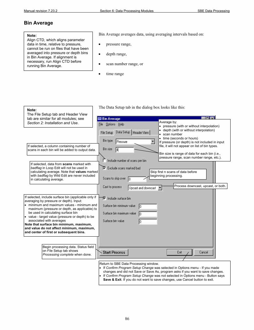
Manual revision 7.23.2 Section 6: Data Processing Modules SBE Data Processing
86
Bin Average Bin Average averages data, using averaging intervals based on: • pressure range, • depth range, • scan number range, or • time range The Data Setup tab in the dialog box looks like this:
Note: Align CTD, which aligns parameter data in time, relative to pressure, cannot be run on files that have been averaged into pressure or depth bins in Bin Average. If alignment is necessary, run Align CTD before running Bin Average.
Average by: • pressure (with or without interpolation) • depth (with or without interpolation) • scan number • time (seconds or hours) If pressure (or depth) is not included in input file, it will not appear on list of bin types. Bin size is range of data for each bin (i.e., pressure range, scan number range, etc.).
If selected, data from scans marked with badflag in Loop Edit will not be used in calculating average. Note that values marked with badflag by Wild Edit are never included in calculating average.
Process downcast, upcast, or both.
If selected, a column containing number of scans in each bin will be added to output data.
If selected, include surface bin (applicable only if averaging by pressure or depth). Input: • minimum and maximum values - minimum and
maximum (pressure or depth, as applicable) to be used in calculating surface bin
• value - target value (pressure or depth) to be associated with averages
Note that surface bin minimum, maximum, and value do not affect minimum, maximum, and center of first or subsequent bins.
Skip first n scans of data before beginning processing.
Return to SBE Data Processing window. • If Confirm Program Setup Change was selected in Options menu - If you made
changes and did not Save or Save As, program asks if you want to save changes. • If Confirm Program Setup Change was not selected in Options menu - Button says
Save & Exit. If you do not want to save changes, use Cancel button to exit.
Begin processing data. Status field on File Setup tab shows Processing complete when done.
Note: The File Setup tab and Header View tab are similar for all modules; see Section 2: Installation and Use.
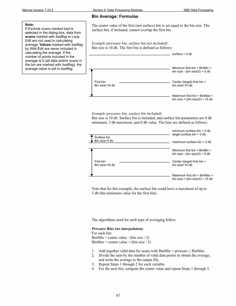
Manual revision 7.23.2 Section 6: Data Processing Modules SBE Data Processing
87
Bin Average: Formulas The center value of the first (not surface) bin is set equal to the bin size. The surface bin, if included, cannot overlap the first bin. Example (pressure bin, surface bin not included): Bin size is 10 db. The first bin is defined as follows:
Example (pressure bin, surface bin included): Bin size is 10 db. Surface bin is included, and surface bin parameters are 0 db minimum, 3 db maximum, and 0 db value. The bins are defined as follows:
Note that for this example, the surface bin could have a maximum of up to 5 db (the minimum value for the first bin). The algorithms used for each type of averaging follow. Pressure Bins (no interpolation) For each bin: BinMin = center value - (bin size / 2) BinMax = center value + (bin size / 2) 1. Add together valid data for scans with BinMin < pressure < BinMax. 2. Divide the sum by the number of valid data points to obtain the average,
and write the average to the output file. 3. Repeat Steps 1 through 2 for each variable. 4. For the next bin, compute the center value and repeat Steps 1 through 3.
Note: If Exclude scans marked bad is selected in the dialog box, data from scans marked with badflag in Loop Edit are not used in calculating average. Values marked with badflag by Wild Edit are never included in calculating the average. If the number of points included in the average is 0 (all data and/or scans in the bin are marked with badflag), the average value is set to badflag.
Center (target) first bin = bin size=10 db
First bin Bin size=10 db
surface = 0 db
Minimum first bin = BinMin = bin size - (bin size/2) = 5 db
Maximum first bin = BinMax = bin size + (bin size/2) = 15 db
Center (target) first bin = bin size=10 db
First bin Bin size=10 db
minimum surface bin = 0 db target surface bin = 0 db
Minimum first bin = BinMin = bin size - (bin size/2) = 5 db
Maximum first bin = BinMax = bin size + (bin size/2) = 15 db
maximum surface bin = 3 db Surface bin Bin size=3 db
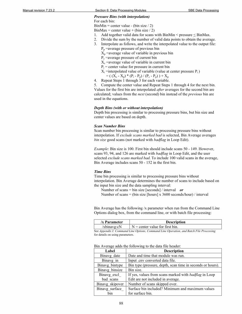
Manual revision 7.23.2 Section 6: Data Processing Modules SBE Data Processing
88
Pressure Bins (with interpolation) For each bin: BinMin = center value - (bin size / 2) BinMax = center value + (bin size / 2) 1. Add together valid data for scans with BinMin < pressure < BinMax. 2. Divide the sum by the number of valid data points to obtain the average. 3. Interpolate as follows, and write the interpolated value to the output file:
Pp =average pressure of previous bin Xp =average value of variable in previous bin Pc =average pressure of current bin Xc =average value of variable in current bin Pi = center value for pressure in current bin Xi =interpolated value of variable (value at center pressure Pi ) = ( (Xc - Xp) * (Pi - Pp) / (Pc - Pp) ) + Xp
4. Repeat Steps 1 through 3 for each variable. 5. Compute the center value and Repeat Steps 1 through 4 for the next bin. Values for the first bin are interpolated after averages for the second bin are calculated; values from the next (second) bin instead of the previous bin are used in the equations. Depth Bins (with or without interpolation) Depth bin processing is similar to processing pressure bins, but bin size and center values are based on depth. Scan Number Bins Scan number bin processing is similar to processing pressure bins without interpolation. If exclude scans marked bad is selected, Bin Average averages bin size good scans (not marked with badflag in Loop Edit). Example: Bin size is 100. First bin should include scans 50 - 149. However, scans 93, 94, and 126 are marked with badflag in Loop Edit, and the user selected exclude scans marked bad. To include 100 valid scans in the average, Bin Average includes scans 50 - 152 in the first bin. Time Bins Time bin processing is similar to processing pressure bins without interpolation. Bin Average determines the number of scans to include based on the input bin size and the data sampling interval:
Number of scans = bin size [seconds] / interval or Number of scans = (bin size [hours] x 3600 seconds/hour) / interval
Bin Average has the following /x parameter when run from the Command Line Options dialog box, from the command line, or with batch file processing:
/x Parameter Description /xbinavg:cN N = center value for first bin.
See Appendix I: Command Line Options, Command Line Operation, and Batch File Processing for details on using parameters. Bin Average adds the following to the data file header:
Label Description Binavg_date Date and time that module was run. Binavg_in Input .cnv converted data file.
Binavg_bintype Bin type (pressure, depth, scan time in seconds or hours). Binavg_binsize Bin size. Binavg_excl_
bad_scans If yes, values from scans marked with badflag in Loop Edit are not included in average.
Binavg_skipover Number of scans skipped over. Binavg_surface_
bin Surface bin included? Minimum and maximum values for surface bin.
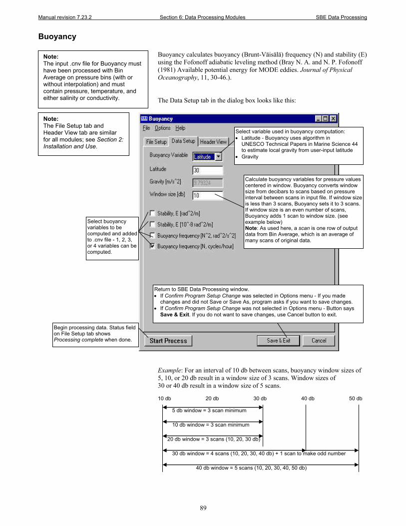
Manual revision 7.23.2 Section 6: Data Processing Modules SBE Data Processing
89
Buoyancy Buoyancy calculates buoyancy (Brunt-Väisälä) frequency (N) and stability (E) using the Fofonoff adiabatic leveling method (Bray N. A. and N. P. Fofonoff (1981) Available potential energy for MODE eddies. Journal of Physical Oceanography, 11, 30-46.). The Data Setup tab in the dialog box looks like this:
Example: For an interval of 10 db between scans, buoyancy window sizes of 5, 10, or 20 db result in a window size of 3 scans. Window sizes of 30 or 40 db result in a window size of 5 scans.
Note: The input .cnv file for Buoyancy must have been processed with Bin Average on pressure bins (with or without interpolation) and must contain pressure, temperature, and either salinity or conductivity.
Select variable used in buoyancy computation: • Latitude - Buoyancy uses algorithm in
UNESCO Technical Papers in Marine Science 44 to estimate local gravity from user-input latitude
• Gravity
Select buoyancy variables to be computed and added to .cnv file - 1, 2, 3, or 4 variables can be computed.
Calculate buoyancy variables for pressure values centered in window. Buoyancy converts window size from decibars to scans based on pressure interval between scans in input file. If window size is less than 3 scans, Buoyancy sets it to 3 scans. If window size is an even number of scans, Buoyancy adds 1 scan to window size. (see example below) Note: As used here, a scan is one row of output data from Bin Average, which is an average of many scans of original data.
Return to SBE Data Processing window. • If Confirm Program Setup Change was selected in Options menu - If you made
changes and did not Save or Save As, program asks if you want to save changes. • If Confirm Program Setup Change was not selected in Options menu - Button says
Save & Exit. If you do not want to save changes, use Cancel button to exit.
Begin processing data. Status field on File Setup tab shows Processing complete when done.
Note: The File Setup tab and Header View tab are similar for all modules; see Section 2: Installation and Use.
40 db window = 5 scans (10, 20, 30, 40, 50 db)
30 db window = 4 scans (10, 20, 30, 40 db) + 1 scan to make odd number
20 db window = 3 scans (10, 20, 30 db)
10 db window = 3 scan minimum
5 db window = 3 scan minimum
10 db 20 db 30 db 40 db 50 db
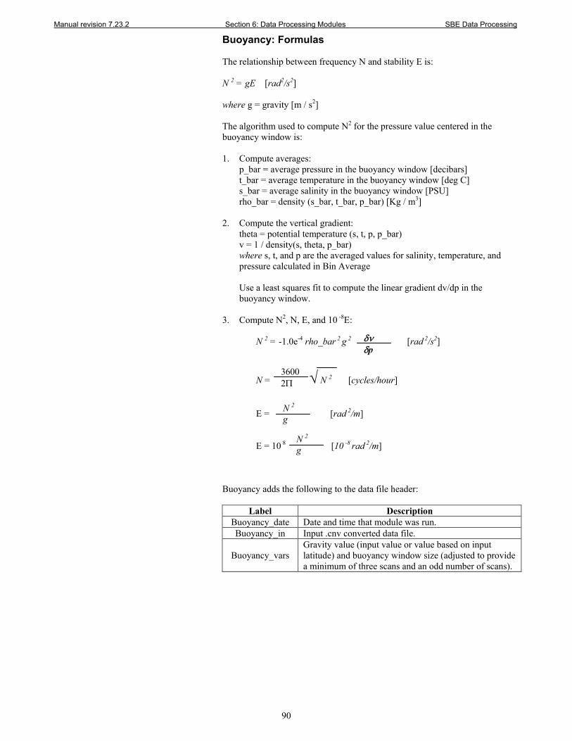
Manual revision 7.23.2 Section 6: Data Processing Modules SBE Data Processing
90
Buoyancy: Formulas The relationship between frequency N and stability E is: N 2 = gE [rad2/s2] where g = gravity [m / s2] The algorithm used to compute N2 for the pressure value centered in the buoyancy window is: 1. Compute averages:
p_bar = average pressure in the buoyancy window [decibars] t_bar = average temperature in the buoyancy window [deg C] s_bar = average salinity in the buoyancy window [PSU] rho_bar = density (s_bar, t_bar, p_bar) [Kg / m3]
2. Compute the vertical gradient:
theta = potential temperature (s, t, p, p_bar) v = 1 / density(s, theta, p_bar) where s, t, and p are the averaged values for salinity, temperature, and pressure calculated in Bin Average
Use a least squares fit to compute the linear gradient dv/dp in the buoyancy window.
3. Compute N2, N, E, and 10 -8E: N 2 = -1.0e-4 rho_bar 2 g 2 [rad 2/s2]
N = √ N 2 [cycles/hour] E = [rad 2/m] E = 10 8 [10 -8 rad 2/m] Buoyancy adds the following to the data file header:
Label Description Buoyancy_date Date and time that module was run. Buoyancy_in Input .cnv converted data file.
Buoyancy_vars Gravity value (input value or value based on input latitude) and buoyancy window size (adjusted to provide a minimum of three scans and an odd number of scans).
N 2 g
3600 2Π
N 2 g
δν δp
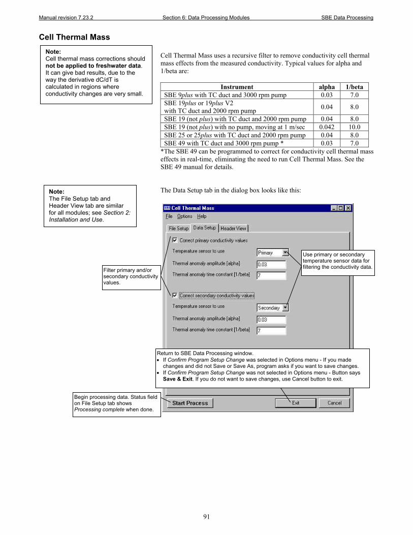
Manual revision 7.23.2 Section 6: Data Processing Modules SBE Data Processing
91
Cell Thermal Mass Cell Thermal Mass uses a recursive filter to remove conductivity cell thermal mass effects from the measured conductivity. Typical values for alpha and 1/beta are:
Instrument alpha 1/beta SBE 9plus with TC duct and 3000 rpm pump 0.03 7.0 SBE 19plus or 19plus V2 with TC duct and 2000 rpm pump 0.04 8.0
SBE 19 (not plus) with TC duct and 2000 rpm pump 0.04 8.0 SBE 19 (not plus) with no pump, moving at 1 m/sec 0.042 10.0 SBE 25 or 25plus with TC duct and 2000 rpm pump 0.04 8.0 SBE 49 with TC duct and 3000 rpm pump * 0.03 7.0
*The SBE 49 can be programmed to correct for conductivity cell thermal mass effects in real-time, eliminating the need to run Cell Thermal Mass. See the SBE 49 manual for details. The Data Setup tab in the dialog box looks like this:
Filter primary and/or secondary conductivity values.
Use primary or secondary temperature sensor data for filtering the conductivity data.
Return to SBE Data Processing window. • If Confirm Program Setup Change was selected in Options menu - If you made
changes and did not Save or Save As, program asks if you want to save changes. • If Confirm Program Setup Change was not selected in Options menu - Button says
Save & Exit. If you do not want to save changes, use Cancel button to exit.
Begin processing data. Status field on File Setup tab shows Processing complete when done.
Note: The File Setup tab and Header View tab are similar for all modules; see Section 2: Installation and Use.
Note: Cell thermal mass corrections should not be applied to freshwater data. It can give bad results, due to the way the derivative dC/dT is calculated in regions where conductivity changes are very small.

Manual revision 7.23.2 Section 6: Data Processing Modules SBE Data Processing
92
Cell Thermal Mass: Formulas The algorithm used is: a = 2 * alpha / (sample interval * beta + 2) b = 1 - (2 * a / alpha) dc/dT = 0.1 * (1 + 0.006 * [temperature - 20]) dT = temperature - previous temperature ctm [S/m] = -1.0 * b * previous ctm + a * (dc/dT) * dT where sample interval is measured in seconds and temperature in °C ctm is calculated in S/m If the input file contains conductivity in units other than S/m, Cell Thermal Mass applies the following scale factors to the calculated ctm: ctm [mS/cm] = ctm [S/m] * 10.0 ctm [µS/cm] = ctm [S/m] * 10000.0 corrected conductivity = c + ctm To determine the values for alpha and beta, see: Lueck, R.G., 1990: Thermal Inertia of Conductivity Cells: Theory., American Meteorological Society Oct 1990, 741-755. Cell Thermal Mass adds the following to the data file header:
Label Description Celltm_date Date and time that module was run. Celltm_in Input .cnv converted data file.
Celltm_alpha Value used for alpha. Celltm_tau Value used for 1/beta.
Celltm_temp_sensor _use_for_cond
Temperature sensor for primary conductivity filter, temperature sensor for secondary conductivity filter.
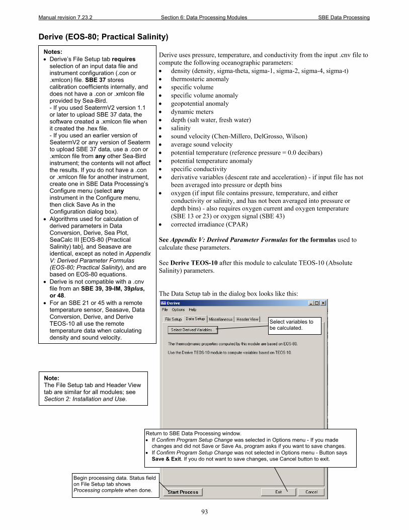
Manual revision 7.23.2 Section 6: Data Processing Modules SBE Data Processing
93
Derive (EOS-80; Practical Salinity) Derive uses pressure, temperature, and conductivity from the input .cnv file to compute the following oceanographic parameters: • density (density, sigma-theta, sigma-1, sigma-2, sigma-4, sigma-t) • thermosteric anomaly • specific volume • specific volume anomaly • geopotential anomaly • dynamic meters • depth (salt water, fresh water) • salinity • sound velocity (Chen-Millero, DelGrosso, Wilson) • average sound velocity • potential temperature (reference pressure = 0.0 decibars) • potential temperature anomaly • specific conductivity • derivative variables (descent rate and acceleration) - if input file has not
been averaged into pressure or depth bins • oxygen (if input file contains pressure, temperature, and either
conductivity or salinity, and has not been averaged into pressure or depth bins) - also requires oxygen current and oxygen temperature (SBE 13 or 23) or oxygen signal (SBE 43)
• corrected irradiance (CPAR) See Appendix V: Derived Parameter Formulas for the formulas used to calculate these parameters. See Derive TEOS-10 after this module to calculate TEOS-10 (Absolute Salinity) parameters. The Data Setup tab in the dialog box looks like this:
Notes: • Derive’s File Setup tab requires
selection of an input data file and instrument configuration (.con or .xmlcon) file. SBE 37 stores calibration coefficients internally, and does not have a .con or .xmlcon file provided by Sea-Bird. - If you used SeatermV2 version 1.1 or later to upload SBE 37 data, the software created a .xmlcon file when it created the .hex file. - If you used an earlier version of SeatermV2 or any version of Seaterm to upload SBE 37 data, use a .con or .xmlcon file from any other Sea-Bird instrument; the contents will not affect the results. If you do not have a .con or .xmlcon file for another instrument, create one in SBE Data Processing’s Configure menu (select any instrument in the Configure menu, then click Save As in the Configuration dialog box).
• Algorithms used for calculation of derived parameters in Data Conversion, Derive, Sea Plot, SeaCalc III [EOS-80 (Practical Salinity) tab], and Seasave are identical, except as noted in Appendix V: Derived Parameter Formulas (EOS-80; Practical Salinity), and are based on EOS-80 equations.
• Derive is not compatible with a .cnv file from an SBE 39, 39-IM, 39plus, or 48.
• For an SBE 21 or 45 with a remote temperature sensor, Seasave, Data Conversion, Derive, and Derive TEOS-10 all use the remote temperature data when calculating density and sound velocity.
Note: The File Setup tab and Header View tab are similar for all modules; see Section 2: Installation and Use.
Select variables to be calculated.
Return to SBE Data Processing window. • If Confirm Program Setup Change was selected in Options menu - If you made
changes and did not Save or Save As, program asks if you want to save changes. • If Confirm Program Setup Change was not selected in Options menu - Button says
Save & Exit. If you do not want to save changes, use Cancel button to exit.
Begin processing data. Status field on File Setup tab shows Processing complete when done.
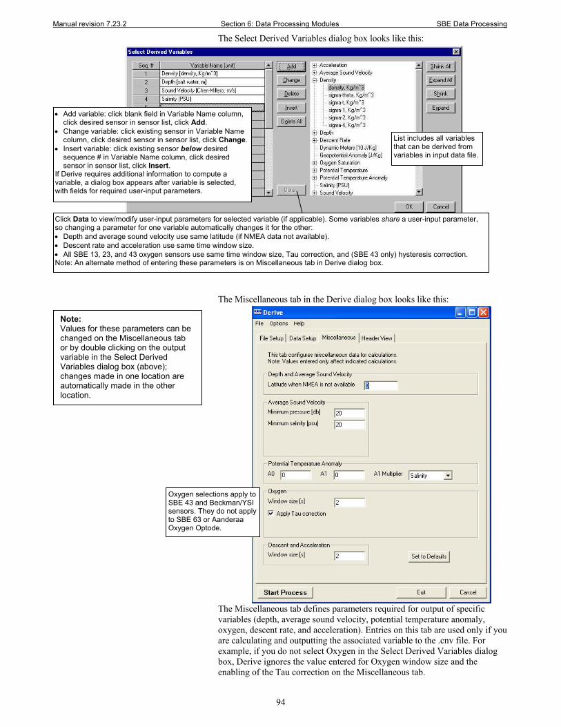
Manual revision 7.23.2 Section 6: Data Processing Modules SBE Data Processing
94
The Select Derived Variables dialog box looks like this:
The Miscellaneous tab in the Derive dialog box looks like this:
The Miscellaneous tab defines parameters required for output of specific variables (depth, average sound velocity, potential temperature anomaly, oxygen, descent rate, and acceleration). Entries on this tab are used only if you are calculating and outputting the associated variable to the .cnv file. For example, if you do not select Oxygen in the Select Derived Variables dialog box, Derive ignores the value entered for Oxygen window size and the enabling of the Tau correction on the Miscellaneous tab.
Note: Values for these parameters can be changed on the Miscellaneous tab or by double clicking on the output variable in the Select Derived Variables dialog box (above); changes made in one location are automatically made in the other location.
Oxygen selections apply to SBE 43 and Beckman/YSI sensors. They do not apply to SBE 63 or Aanderaa Oxygen Optode.
Click Data to view/modify user-input parameters for selected variable (if applicable). Some variables share a user-input parameter, so changing a parameter for one variable automatically changes it for the other: • Depth and average sound velocity use same latitude (if NMEA data not available). • Descent rate and acceleration use same time window size. • All SBE 13, 23, and 43 oxygen sensors use same time window size, Tau correction, and (SBE 43 only) hysteresis correction. Note: An alternate method of entering these parameters is on Miscellaneous tab in Derive dialog box.
• Add variable: click blank field in Variable Name column, click desired sensor in sensor list, click Add.
• Change variable: click existing sensor in Variable Name column, click desired sensor in sensor list, click Change.
• Insert variable: click existing sensor below desired sequence # in Variable Name column, click desired sensor in sensor list, click Insert.
If Derive requires additional information to compute a variable, a dialog box appears after variable is selected, with fields for required user-input parameters.
List includes all variables that can be derived from variables in input data file.
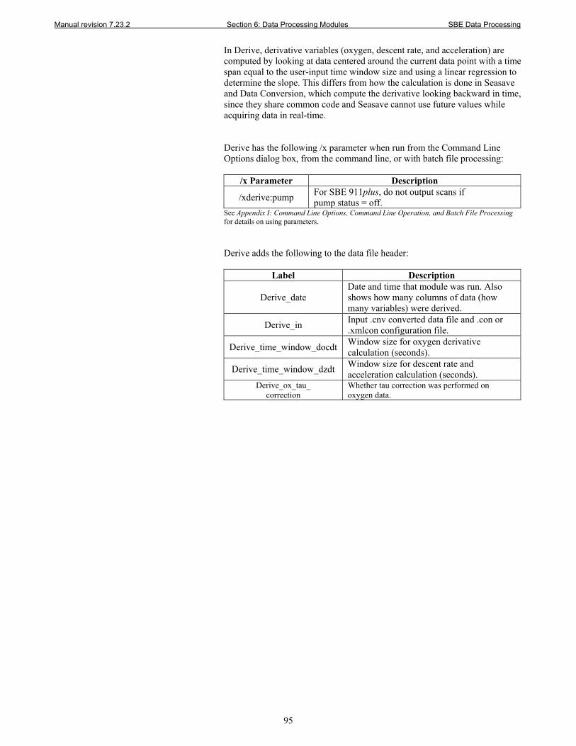
Manual revision 7.23.2 Section 6: Data Processing Modules SBE Data Processing
95
In Derive, derivative variables (oxygen, descent rate, and acceleration) are computed by looking at data centered around the current data point with a time span equal to the user-input time window size and using a linear regression to determine the slope. This differs from how the calculation is done in Seasave and Data Conversion, which compute the derivative looking backward in time, since they share common code and Seasave cannot use future values while acquiring data in real-time. Derive has the following /x parameter when run from the Command Line Options dialog box, from the command line, or with batch file processing:
/x Parameter Description
/xderive:pump For SBE 911plus, do not output scans if pump status = off.
See Appendix I: Command Line Options, Command Line Operation, and Batch File Processing for details on using parameters. Derive adds the following to the data file header:
Label Description
Derive_date Date and time that module was run. Also shows how many columns of data (how many variables) were derived.
Derive_in Input .cnv converted data file and .con or .xmlcon configuration file.
Derive_time_window_docdt Window size for oxygen derivative calculation (seconds).
Derive_time_window_dzdt Window size for descent rate and acceleration calculation (seconds).
Derive_ox_tau_ correction
Whether tau correction was performed on oxygen data.
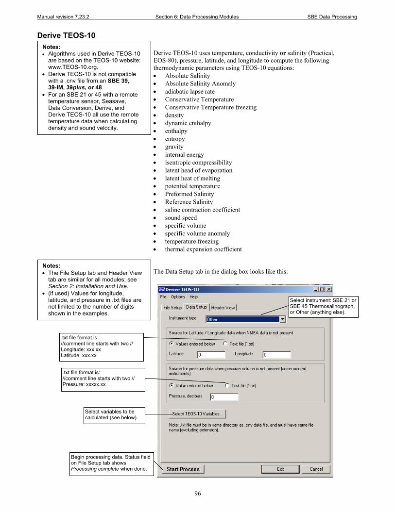
Manual revision 7.23.2 Section 6: Data Processing Modules SBE Data Processing
96
Derive TEOS-10 Derive TEOS-10 uses temperature, conductivity or salinity (Practical, EOS-80), pressure, latitude, and longitude to compute the following thermodynamic parameters using TEOS-10 equations: • Absolute Salinity • Absolute Salinity Anomaly • adiabatic lapse rate • Conservative Temperature • Conservative Temperature freezing • density • dynamic enthalpy • enthalpy • entropy • gravity • internal energy • isentropic compressibility • latent head of evaporation • latent heat of melting • potential temperature • Preformed Salinity • Reference Salinity • saline contraction coefficient • sound speed • specific volume • specific volume anomaly • temperature freezing • thermal expansion coefficient The Data Setup tab in the dialog box looks like this:
Notes: • Algorithms used in Derive TEOS-10
are based on the TEOS-10 website: www.TEOS-10.org.
• Derive TEOS-10 is not compatible with a .cnv file from an SBE 39, 39-IM, 39plus, or 48.
• For an SBE 21 or 45 with a remote temperature sensor, Seasave, Data Conversion, Derive, and Derive TEOS-10 all use the remote temperature data when calculating density and sound velocity.
Notes: • The File Setup tab and Header View
tab are similar for all modules; see Section 2: Installation and Use.
• (if used) Values for longitude, latitude, and pressure in .txt files are not limited to the number of digits shown in the examples.
Select variables to be calculated (see below).
Begin processing data. Status field on File Setup tab shows Processing complete when done.
Select instrument: SBE 21 or SBE 45 Thermosalinograph, or Other (anything else).
.txt file format is: //comment line starts with two // Longitude: xxx.xx Latitude: xxx.xx
.txt file format is: //comment line starts with two // Pressure: xxxxx.xx
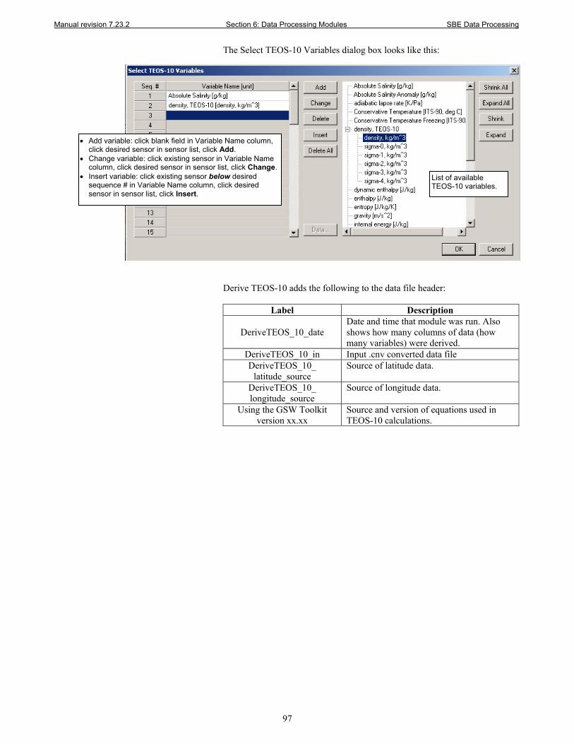
Manual revision 7.23.2 Section 6: Data Processing Modules SBE Data Processing
97
The Select TEOS-10 Variables dialog box looks like this:
Derive TEOS-10 adds the following to the data file header:
Label Description
DeriveTEOS_10_date Date and time that module was run. Also shows how many columns of data (how many variables) were derived.
DeriveTEOS_10_in Input .cnv converted data file DeriveTEOS_10_
latitude_source Source of latitude data.
DeriveTEOS_10_ longitude_source
Source of longitude data.
Using the GSW Toolkit version xx.xx
Source and version of equations used in TEOS-10 calculations.
• Add variable: click blank field in Variable Name column, click desired sensor in sensor list, click Add.
• Change variable: click existing sensor in Variable Name column, click desired sensor in sensor list, click Change.
• Insert variable: click existing sensor below desired sequence # in Variable Name column, click desired sensor in sensor list, click Insert.
List of available TEOS-10 variables.
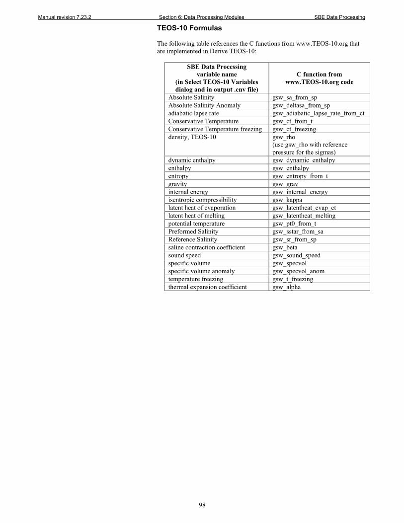
Manual revision 7.23.2 Section 6: Data Processing Modules SBE Data Processing
98
TEOS-10 Formulas The following table references the C functions from www.TEOS-10.org that are implemented in Derive TEOS-10:
SBE Data Processing variable name
(in Select TEOS-10 Variables dialog and in output .cnv file)
C function from www.TEOS-10.org code
Absolute Salinity gsw_sa_from_sp Absolute Salinity Anomaly gsw_deltasa_from_sp adiabatic lapse rate gsw_adiabatic_lapse_rate_from_ct Conservative Temperature gsw_ct_from_t Conservative Temperature freezing gsw_ct_freezing density, TEOS-10 gsw_rho
(use gsw_rho with reference pressure for the sigmas)
dynamic enthalpy gsw_dynamic_enthalpy enthalpy gsw_enthalpy entropy gsw_entropy_from_t gravity gsw_grav internal energy gsw_internal_energy isentropic compressibility gsw_kappa latent heat of evaporation gsw_latentheat_evap_ct latent heat of melting gsw_latentheat_melting potential temperature gsw_pt0_from_t Preformed Salinity gsw_sstar_from_sa Reference Salinity gsw_sr_from_sp saline contraction coefficient gsw_beta sound speed gsw_sound_speed specific volume gsw_specvol specific volume anomaly gsw_specvol_anom temperature freezing gsw_t_freezing thermal expansion coefficient gsw_alpha
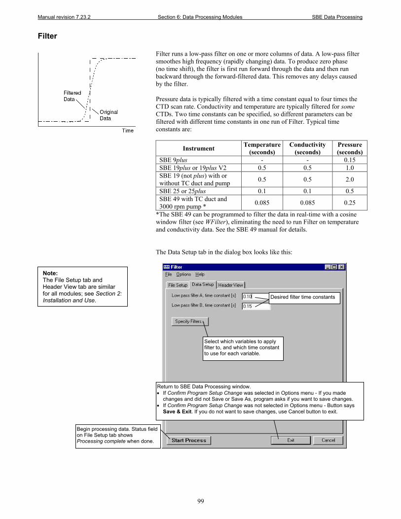
Manual revision 7.23.2 Section 6: Data Processing Modules SBE Data Processing
99
Filter Filter runs a low-pass filter on one or more columns of data. A low-pass filter smoothes high frequency (rapidly changing) data. To produce zero phase (no time shift), the filter is first run forward through the data and then run backward through the forward-filtered data. This removes any delays caused by the filter. Pressure data is typically filtered with a time constant equal to four times the CTD scan rate. Conductivity and temperature are typically filtered for some CTDs. Two time constants can be specified, so different parameters can be filtered with different time constants in one run of Filter. Typical time constants are:
Instrument Temperature (seconds)
Conductivity (seconds)
Pressure (seconds)
SBE 9plus - - 0.15 SBE 19plus or 19plus V2 0.5 0.5 1.0 SBE 19 (not plus) with or without TC duct and pump 0.5 0.5 2.0
SBE 25 or 25plus 0.1 0.1 0.5 SBE 49 with TC duct and 3000 rpm pump * 0.085 0.085 0.25
*The SBE 49 can be programmed to filter the data in real-time with a cosine window filter (see WFilter), eliminating the need to run Filter on temperature and conductivity data. See the SBE 49 manual for details. The Data Setup tab in the dialog box looks like this:
Select which variables to apply filter to, and which time constant to use for each variable.
Desired filter time constants
Return to SBE Data Processing window. • If Confirm Program Setup Change was selected in Options menu - If you made
changes and did not Save or Save As, program asks if you want to save changes. • If Confirm Program Setup Change was not selected in Options menu - Button says
Save & Exit. If you do not want to save changes, use Cancel button to exit.
Begin processing data. Status field on File Setup tab shows Processing complete when done.
Note: The File Setup tab and Header View tab are similar for all modules; see Section 2: Installation and Use.
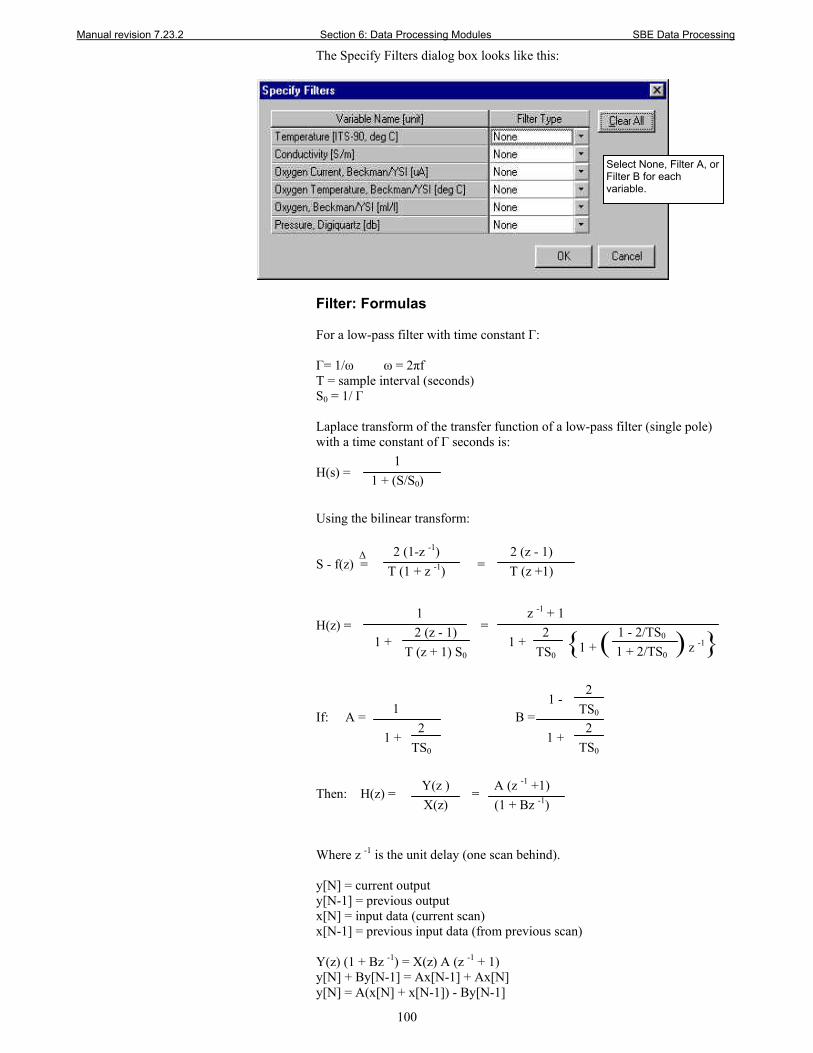
Manual revision 7.23.2 Section 6: Data Processing Modules SBE Data Processing
100
The Specify Filters dialog box looks like this:
Filter: Formulas For a low-pass filter with time constant Γ: Γ= 1/ω ω = 2πf T = sample interval (seconds) S0 = 1/ Γ Laplace transform of the transfer function of a low-pass filter (single pole) with a time constant of Γ seconds is: H(s) = Using the bilinear transform: S - f(z) = = H(z) = = If: A = B = Then: H(z) = = Where z -1 is the unit delay (one scan behind). y[N] = current output y[N-1] = previous output x[N] = input data (current scan) x[N-1] = previous input data (from previous scan) Y(z) (1 + Bz -1) = X(z) A (z -1 + 1) y[N] + By[N-1] = Ax[N-1] + Ax[N] y[N] = A(x[N] + x[N-1]) - By[N-1]
1 1 + (S/S0)
2 (1-z -1) T (1 + z -1)
2 (z - 1) T (z +1)
Δ
1 2 (z - 1)
T (z + 1) S0 1 +
z -1 + 1 2
TS0 1 + {1 + ( ) z -1} 1 - 2/TS0
1 + 2/TS0
1 2
TS0 1 +
2 TS0
1 +
2 TS0
1 -
A (z -1 +1) (1 + Bz -1)
Y(z ) X(z)
Select None, Filter A, or Filter B for each variable.
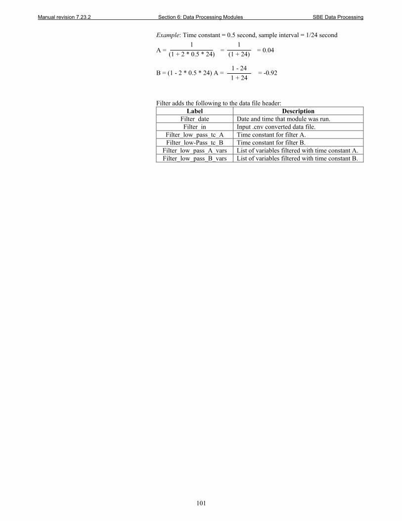
Manual revision 7.23.2 Section 6: Data Processing Modules SBE Data Processing
101
Example: Time constant = 0.5 second, sample interval = 1/24 second A = = = 0.04 B = (1 - 2 * 0.5 * 24) A = = -0.92 Filter adds the following to the data file header:
Label Description Filter_date Date and time that module was run. Filter_in Input .cnv converted data file.
Filter_low_pass_tc_A Time constant for filter A. Filter_low-Pass_tc_B Time constant for filter B.
Filter_low_pass_A_vars List of variables filtered with time constant A. Filter_low_pass_B_vars List of variables filtered with time constant B.
1 (1 + 2 * 0.5 * 24)
1 (1 + 24)
1 - 24 1 + 24
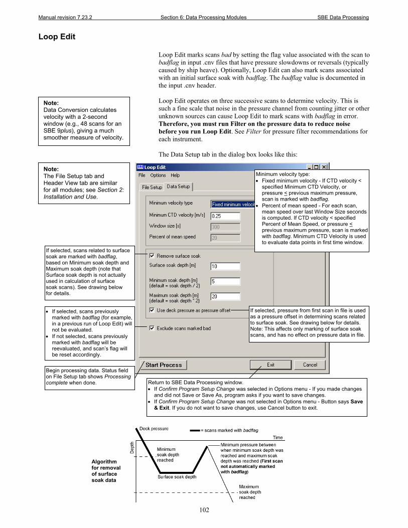
Manual revision 7.23.2 Section 6: Data Processing Modules SBE Data Processing
102
Loop Edit Loop Edit marks scans bad by setting the flag value associated with the scan to badflag in input .cnv files that have pressure slowdowns or reversals (typically caused by ship heave). Optionally, Loop Edit can also mark scans associated with an initial surface soak with badflag. The badflag value is documented in the input .cnv header. Loop Edit operates on three successive scans to determine velocity. This is such a fine scale that noise in the pressure channel from counting jitter or other unknown sources can cause Loop Edit to mark scans with badflag in error. Therefore, you must run Filter on the pressure data to reduce noise before you run Loop Edit. See Filter for pressure filter recommendations for each instrument. The Data Setup tab in the dialog box looks like this:
Note: Data Conversion calculates velocity with a 2-second window (e.g., 48 scans for an SBE 9plus), giving a much smoother measure of velocity.
Note: The File Setup tab and Header View tab are similar for all modules; see Section 2: Installation and Use.
• If selected, scans previously marked with badflag (for example, in a previous run of Loop Edit) will not be evaluated.
• If not selected, scans previously marked with badflag will be reevaluated, and scan’s flag will be reset accordingly.
Minimum velocity type: • Fixed minimum velocity - If CTD velocity <
specified Minimum CTD Velocity, or pressure < previous maximum pressure, scan is marked with badflag.
• Percent of mean speed - For each scan, mean speed over last Window Size seconds is computed. If CTD velocity < specified Percent of Mean Speed, or pressure < previous maximum pressure, scan is marked with badflag. Minimum CTD Velocity is used to evaluate data points in first time window.
Return to SBE Data Processing window. • If Confirm Program Setup Change was selected in Options menu - If you made changes
and did not Save or Save As, program asks if you want to save changes. • If Confirm Program Setup Change was not selected in Options menu - Button says Save
& Exit. If you do not want to save changes, use Cancel button to exit.
Begin processing data. Status field on File Setup tab shows Processing complete when done.
If selected, scans related to surface soak are marked with badflag, based on Minimum soak depth and Maximum soak depth (note that Surface soak depth is not actually used in calculation of surface soak scans). See drawing below for details.
If selected, pressure from first scan in file is used as a pressure offset in determining scans related to surface soak. See drawing below for details. Note: This affects only marking of surface soak scans, and has no effect on pressure data in file.
Algorithm for removal of surface soak data
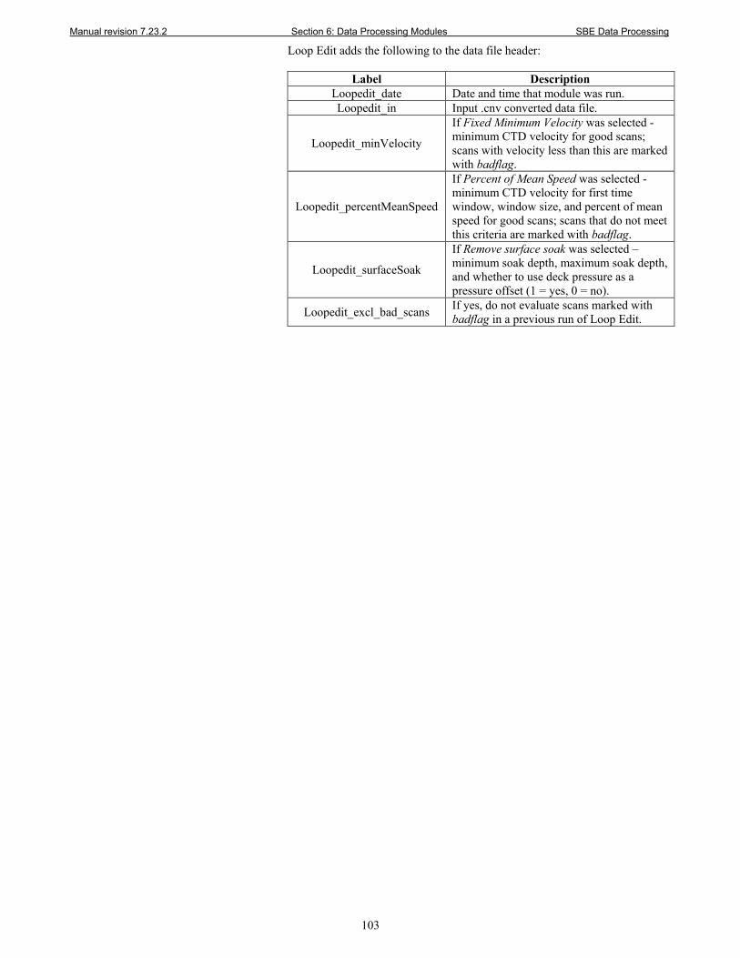
Manual revision 7.23.2 Section 6: Data Processing Modules SBE Data Processing
103
Loop Edit adds the following to the data file header:
Label Description Loopedit_date Date and time that module was run. Loopedit_in Input .cnv converted data file.
Loopedit_minVelocity
If Fixed Minimum Velocity was selected - minimum CTD velocity for good scans; scans with velocity less than this are marked with badflag.
Loopedit_percentMeanSpeed
If Percent of Mean Speed was selected - minimum CTD velocity for first time window, window size, and percent of mean speed for good scans; scans that do not meet this criteria are marked with badflag.
Loopedit_surfaceSoak
If Remove surface soak was selected – minimum soak depth, maximum soak depth, and whether to use deck pressure as a pressure offset (1 = yes, 0 = no).
Loopedit_excl_bad_scans If yes, do not evaluate scans marked with badflag in a previous run of Loop Edit.
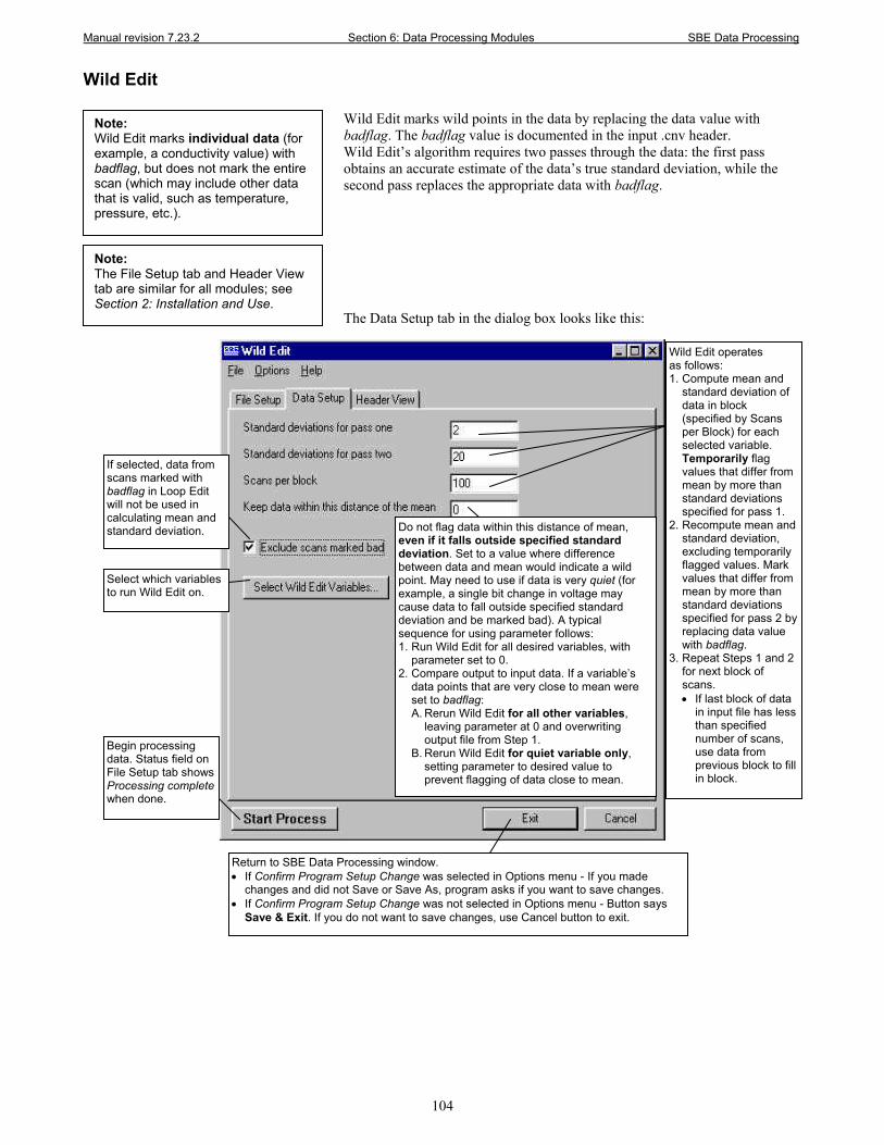
Manual revision 7.23.2 Section 6: Data Processing Modules SBE Data Processing
104
Wild Edit Wild Edit marks wild points in the data by replacing the data value with badflag. The badflag value is documented in the input .cnv header. Wild Edit’s algorithm requires two passes through the data: the first pass obtains an accurate estimate of the data’s true standard deviation, while the second pass replaces the appropriate data with badflag. The Data Setup tab in the dialog box looks like this:
Note: Wild Edit marks individual data (for example, a conductivity value) with badflag, but does not mark the entire scan (which may include other data that is valid, such as temperature, pressure, etc.).
If selected, data from scans marked with badflag in Loop Edit will not be used in calculating mean and standard deviation.
Select which variables to run Wild Edit on.
Wild Edit operates as follows: 1. Compute mean and
standard deviation of data in block (specified by Scans per Block) for each selected variable. Temporarily flag values that differ from mean by more than standard deviations specified for pass 1.
2. Recompute mean and standard deviation, excluding temporarily flagged values. Mark values that differ from mean by more than standard deviations specified for pass 2 by replacing data value with badflag.
3. Repeat Steps 1 and 2 for next block of scans. • If last block of data
in input file has less than specified number of scans, use data from previous block to fill in block.
Do not flag data within this distance of mean, even if it falls outside specified standard deviation. Set to a value where difference between data and mean would indicate a wild point. May need to use if data is very quiet (for example, a single bit change in voltage may cause data to fall outside specified standard deviation and be marked bad). A typical sequence for using parameter follows: 1. Run Wild Edit for all desired variables, with
parameter set to 0. 2. Compare output to input data. If a variable’s
data points that are very close to mean were set to badflag: A. Rerun Wild Edit for all other variables,
leaving parameter at 0 and overwriting output file from Step 1.
B. Rerun Wild Edit for quiet variable only, setting parameter to desired value to prevent flagging of data close to mean.
Return to SBE Data Processing window. • If Confirm Program Setup Change was selected in Options menu - If you made
changes and did not Save or Save As, program asks if you want to save changes. • If Confirm Program Setup Change was not selected in Options menu - Button says
Save & Exit. If you do not want to save changes, use Cancel button to exit.
Begin processing data. Status field on File Setup tab shows Processing complete when done.
Note: The File Setup tab and Header View tab are similar for all modules; see Section 2: Installation and Use.
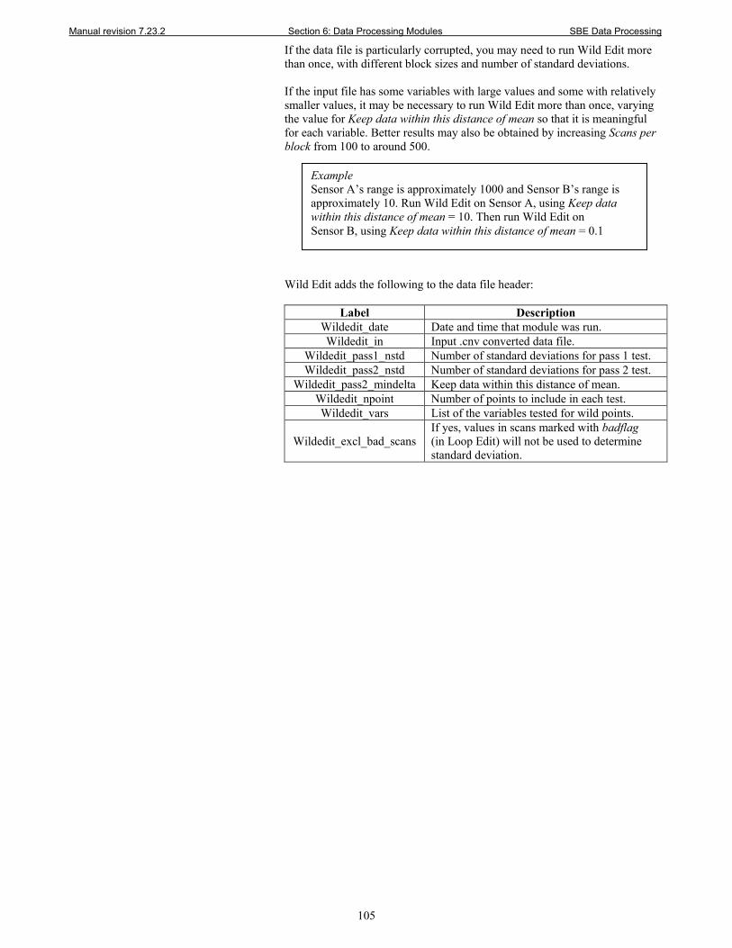
Manual revision 7.23.2 Section 6: Data Processing Modules SBE Data Processing
105
If the data file is particularly corrupted, you may need to run Wild Edit more than once, with different block sizes and number of standard deviations. If the input file has some variables with large values and some with relatively smaller values, it may be necessary to run Wild Edit more than once, varying the value for Keep data within this distance of mean so that it is meaningful for each variable. Better results may also be obtained by increasing Scans per block from 100 to around 500.
Wild Edit adds the following to the data file header:
Label Description
Wildedit_date Date and time that module was run. Wildedit_in Input .cnv converted data file.
Wildedit_pass1_nstd Number of standard deviations for pass 1 test. Wildedit_pass2_nstd Number of standard deviations for pass 2 test.
Wildedit_pass2_mindelta Keep data within this distance of mean. Wildedit_npoint Number of points to include in each test. Wildedit_vars List of the variables tested for wild points.
Wildedit_excl_bad_scans If yes, values in scans marked with badflag (in Loop Edit) will not be used to determine standard deviation.
Example Sensor A’s range is approximately 1000 and Sensor B’s range is approximately 10. Run Wild Edit on Sensor A, using Keep data within this distance of mean = 10. Then run Wild Edit on Sensor B, using Keep data within this distance of mean = 0.1
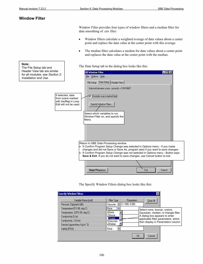
Manual revision 7.23.2 Section 6: Data Processing Modules SBE Data Processing
106
Window Filter Window Filter provides four types of window filters and a median filter for data smoothing of .cnv files: • Window filters calculate a weighted average of data values about a center
point and replace the data value at the center point with this average. • The median filter calculates a median for data values about a center point
and replaces the data value at the center point with the median. The Data Setup tab in the dialog box looks like this:
The Specify Window Filters dialog box looks like this:
Select none, boxcar, cosine, Gaussian, median, or triangle filter. A dialog box appears to enter applicable filter parameters, which then display in Parameters column.
If selected, data from scans marked with badflag in Loop Edit will not be used.
Select which variables to run Window Filter on, and specify the filters.
Return to SBE Data Processing window. • If Confirm Program Setup Change was selected in Options menu - If you made
changes and did not Save or Save As, program asks if you want to save changes. • If Confirm Program Setup Change was not selected in Options menu - Button says
Save & Exit. If you do not want to save changes, use Cancel button to exit.
Note: The File Setup tab and Header View tab are similar for all modules; see Section 2: Installation and Use.
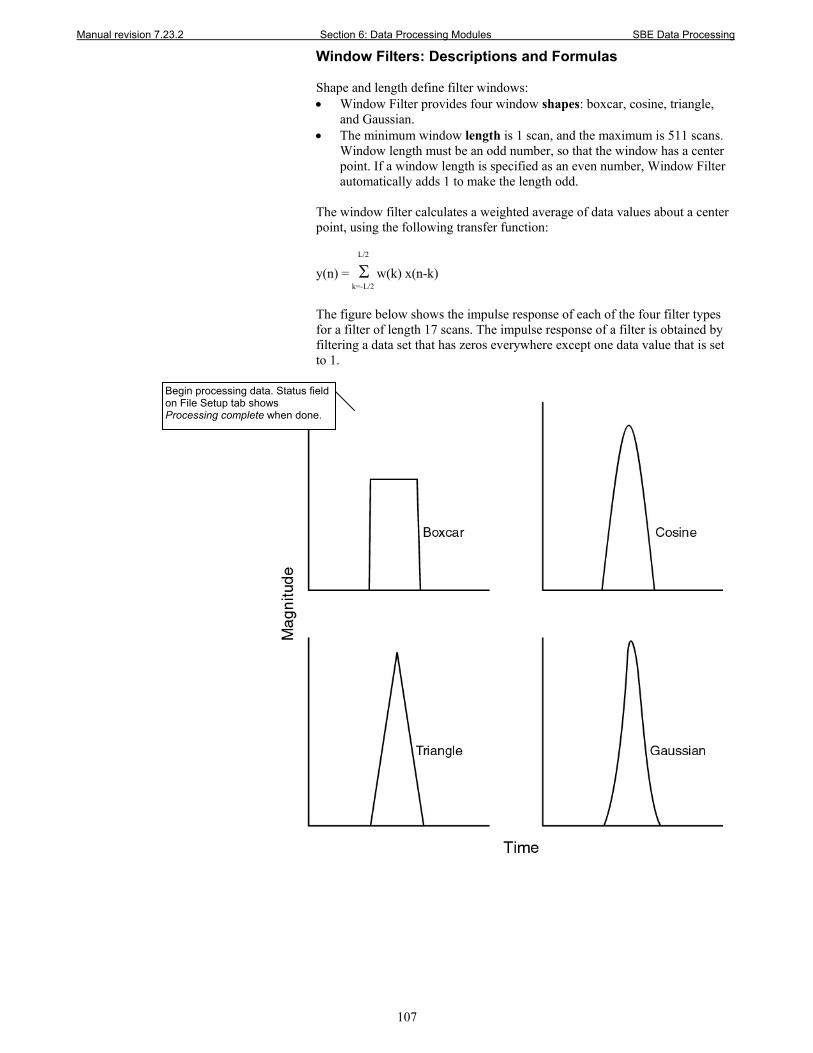
Manual revision 7.23.2 Section 6: Data Processing Modules SBE Data Processing
107
Window Filters: Descriptions and Formulas Shape and length define filter windows: • Window Filter provides four window shapes: boxcar, cosine, triangle,
and Gaussian. • The minimum window length is 1 scan, and the maximum is 511 scans.
Window length must be an odd number, so that the window has a center point. If a window length is specified as an even number, Window Filter automatically adds 1 to make the length odd.
The window filter calculates a weighted average of data values about a center point, using the following transfer function: L/2
y(n) = Σ w(k) x(n-k) k=-L/2
The figure below shows the impulse response of each of the four filter types for a filter of length 17 scans. The impulse response of a filter is obtained by filtering a data set that has zeros everywhere except one data value that is set to 1.
Begin processing data. Status field on File Setup tab shows Processing complete when done.
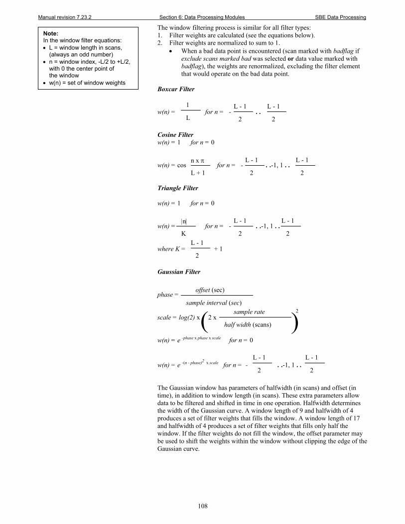
Manual revision 7.23.2 Section 6: Data Processing Modules SBE Data Processing
108
The window filtering process is similar for all filter types: 1. Filter weights are calculated (see the equations below). 2. Filter weights are normalized to sum to 1.
• When a bad data point is encountered (scan marked with badflag if exclude scans marked bad was selected or data value marked with badflag), the weights are renormalized, excluding the filter element that would operate on the bad data point.
Boxcar Filter w(n) = for n = - . . Cosine Filter w(n) = 1 for n = 0 w(n) = cos for n = - . .-1, 1 . . Triangle Filter w(n) = 1 for n = 0 w(n) = for n = - . .-1, 1 . . where K = + 1 Gaussian Filter phase = scale = log(2) x 2 x w(n) = e -phase x phase x scale for n = 0 w(n) = e -(n - phase)2 x scale for n = - . .-1, 1 . . The Gaussian window has parameters of halfwidth (in scans) and offset (in time), in addition to window length (in scans). These extra parameters allow data to be filtered and shifted in time in one operation. Halfwidth determines the width of the Gaussian curve. A window length of 9 and halfwidth of 4 produces a set of filter weights that fills the window. A window length of 17 and halfwidth of 4 produces a set of filter weights that fills only half the window. If the filter weights do not fill the window, the offset parameter may be used to shift the weights within the window without clipping the edge of the Gaussian curve.
Note: In the window filter equations: • L = window length in scans,
(always an odd number) • n = window index, -L/2 to +L/2,
with 0 the center point of the window
• w(n) = set of window weights
1
L
L - 1
2
L - 1
2
n x π
L + 1
L - 1
2
L - 1
2
|n|
K
L - 1
2
L - 1
2 L - 1
2
offset (sec)
sample interval (sec) sample rate
half width (scans) ( ) 2
L - 1
2
L - 1
2
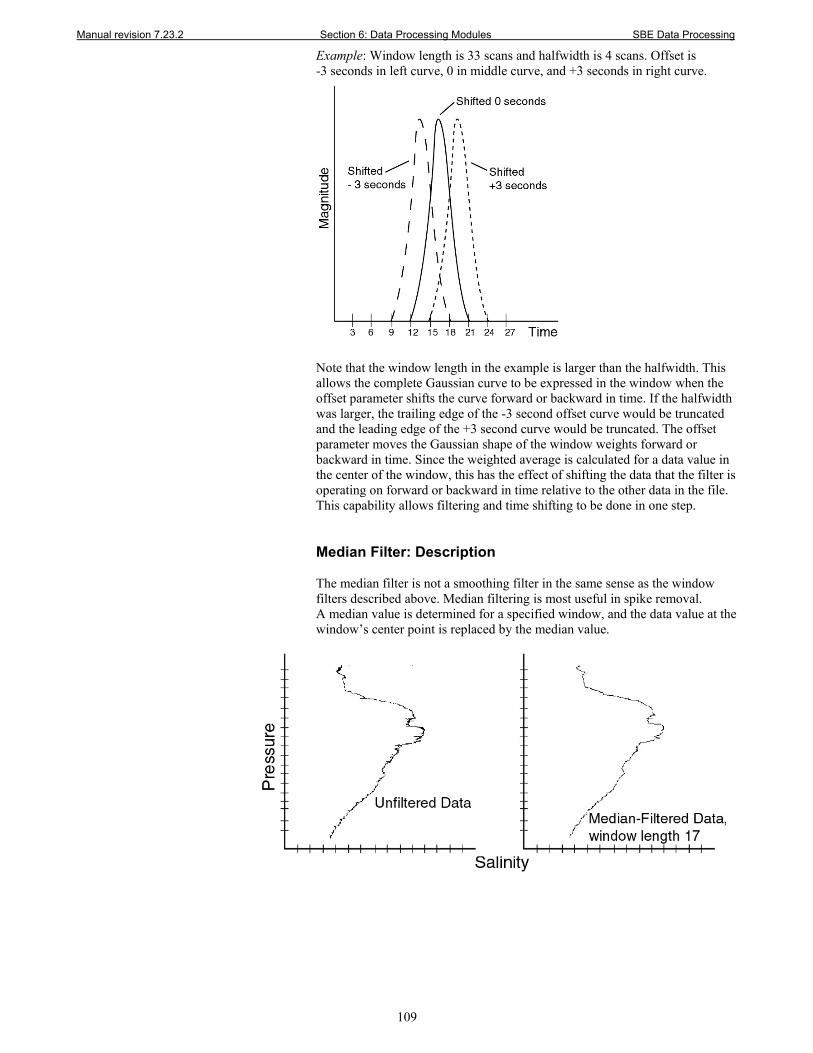
Manual revision 7.23.2 Section 6: Data Processing Modules SBE Data Processing
109
Example: Window length is 33 scans and halfwidth is 4 scans. Offset is -3 seconds in left curve, 0 in middle curve, and +3 seconds in right curve.
Note that the window length in the example is larger than the halfwidth. This allows the complete Gaussian curve to be expressed in the window when the offset parameter shifts the curve forward or backward in time. If the halfwidth was larger, the trailing edge of the -3 second offset curve would be truncated and the leading edge of the +3 second curve would be truncated. The offset parameter moves the Gaussian shape of the window weights forward or backward in time. Since the weighted average is calculated for a data value in the center of the window, this has the effect of shifting the data that the filter is operating on forward or backward in time relative to the other data in the file. This capability allows filtering and time shifting to be done in one step. Median Filter: Description The median filter is not a smoothing filter in the same sense as the window filters described above. Median filtering is most useful in spike removal. A median value is determined for a specified window, and the data value at the window’s center point is replaced by the median value.
Manual revision 7.23.2 Section 6: Data Processing Modules SBE Data Processing
110
Window Filter has the following /x parameter when run from the Command Line Options dialog box, from the command line, or with batch file processing:
/x Parameter Description
/xwfilter:diff Output difference between original and filtered value instead of outputting filtered value.
See Appendix I: Command Line Options, Command Line Operation, and Batch File Processing for details on using parameters. Window Filter adds the following to the data file header:
Label Description Wfilter_date Date and time that module was run. Wfilter_in Input .cnv converted data file.
Wfilter_excl_ bad_scans
If yes, values in scans marked with badflag in Loop Edit will not be used.
Wfilter_action Data channel identifier, filter type, filter parameters.
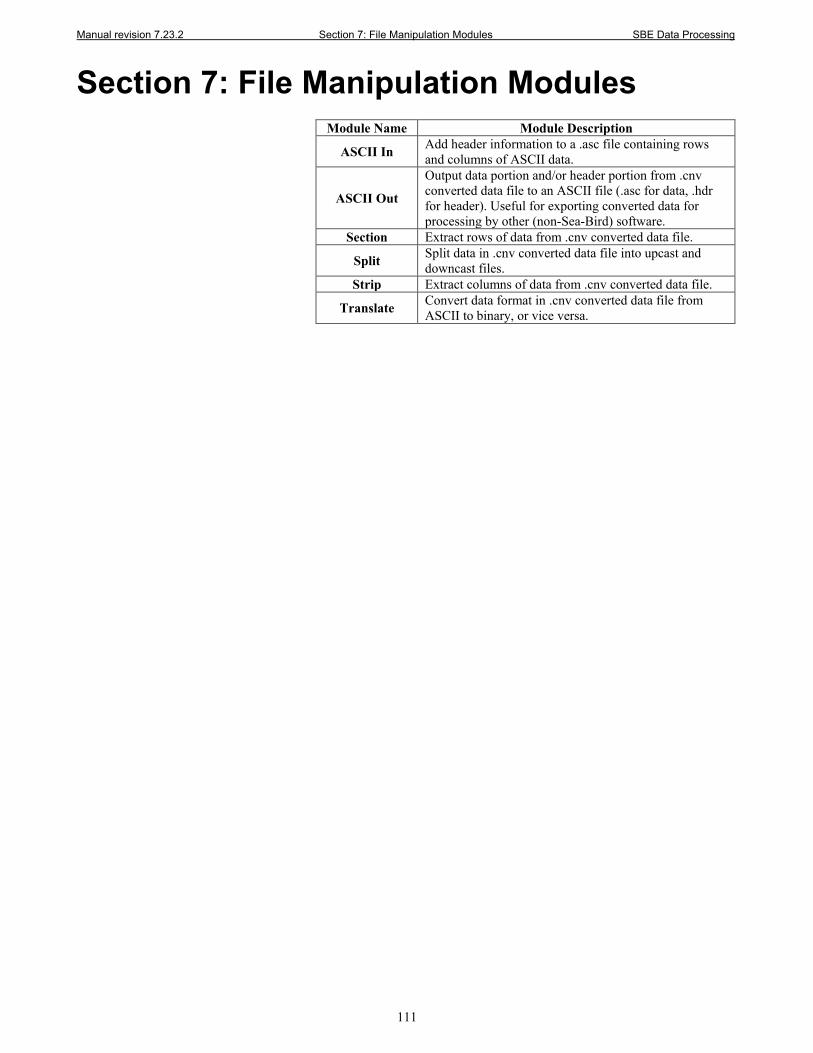
Manual revision 7.23.2 Section 7: File Manipulation Modules SBE Data Processing
111
Section 7: File Manipulation Modules
Module Name Module Description
ASCII In Add header information to a .asc file containing rows and columns of ASCII data.
ASCII Out
Output data portion and/or header portion from .cnv converted data file to an ASCII file (.asc for data, .hdr for header). Useful for exporting converted data for processing by other (non-Sea-Bird) software.
Section Extract rows of data from .cnv converted data file.
Split Split data in .cnv converted data file into upcast and downcast files.
Strip Extract columns of data from .cnv converted data file.
Translate Convert data format in .cnv converted data file from ASCII to binary, or vice versa.
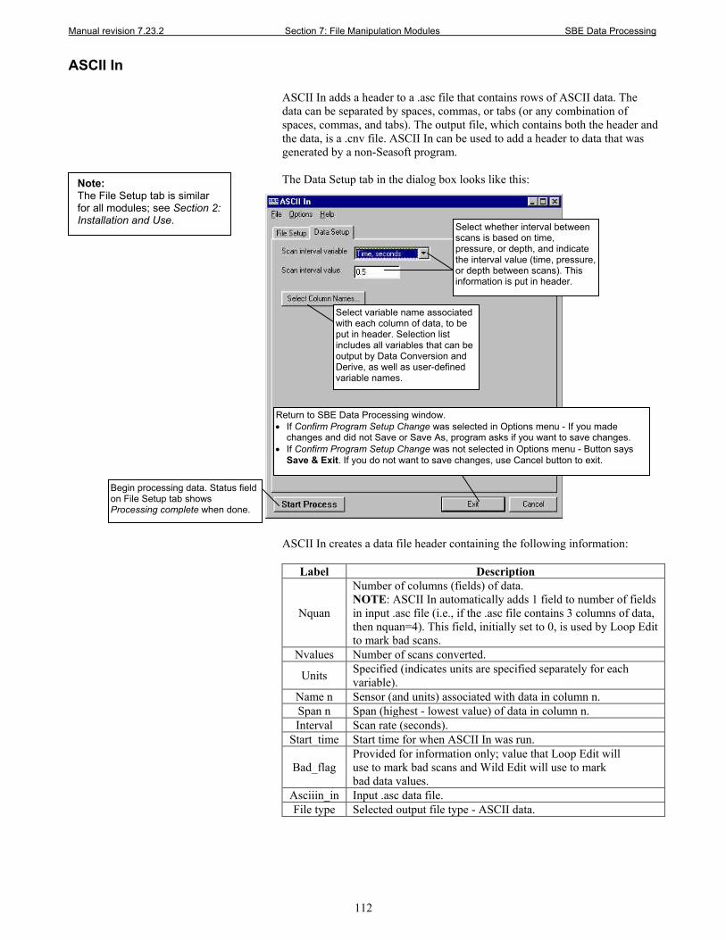
Manual revision 7.23.2 Section 7: File Manipulation Modules SBE Data Processing
112
ASCII In ASCII In adds a header to a .asc file that contains rows of ASCII data. The data can be separated by spaces, commas, or tabs (or any combination of spaces, commas, and tabs). The output file, which contains both the header and the data, is a .cnv file. ASCII In can be used to add a header to data that was generated by a non-Seasoft program. The Data Setup tab in the dialog box looks like this:
ASCII In creates a data file header containing the following information:
Label Description
Nquan
Number of columns (fields) of data. NOTE: ASCII In automatically adds 1 field to number of fields in input .asc file (i.e., if the .asc file contains 3 columns of data, then nquan=4). This field, initially set to 0, is used by Loop Edit to mark bad scans.
Nvalues Number of scans converted.
Units Specified (indicates units are specified separately for each variable).
Name n Sensor (and units) associated with data in column n. Span n Span (highest - lowest value) of data in column n. Interval Scan rate (seconds).
Start_time Start time for when ASCII In was run.
Bad_flag Provided for information only; value that Loop Edit will use to mark bad scans and Wild Edit will use to mark bad data values.
Asciiin_in Input .asc data file. File type Selected output file type - ASCII data.
Select variable name associated with each column of data, to be put in header. Selection list includes all variables that can be output by Data Conversion and Derive, as well as user-defined variable names.
Select whether interval between scans is based on time, pressure, or depth, and indicate the interval value (time, pressure, or depth between scans). This information is put in header.
Return to SBE Data Processing window. • If Confirm Program Setup Change was selected in Options menu - If you made
changes and did not Save or Save As, program asks if you want to save changes. • If Confirm Program Setup Change was not selected in Options menu - Button says
Save & Exit. If you do not want to save changes, use Cancel button to exit.
Begin processing data. Status field on File Setup tab shows Processing complete when done.
Note: The File Setup tab is similar for all modules; see Section 2: Installation and Use.
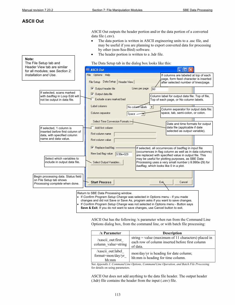
Manual revision 7.23.2 Section 7: File Manipulation Modules SBE Data Processing
113
ASCII Out ASCII Out outputs the header portion and/or the data portion of a converted data file (.cnv). • The data portion is written in ASCII engineering units to a .asc file, and
may be useful if you are planning to export converted data for processing by other (non-Sea-Bird) software.
• The header portion is written to a .hdr file. The Data Setup tab in the dialog box looks like this:
ASCII Out has the following /x parameter when run from the Command Line Options dialog box, from the command line, or with batch file processing:
/x Parameter Description
/xascii_out:first_ column_value=string
string = value (maximum of 11 characters) placed in each row of column inserted before first column of data.
/xascii_out:label_ format=mon/day/yr_
hh:mm
mon/day/yr is heading for date column; hh:mm is heading for time column.
See Appendix I: Command Line Options, Command Line Operation, and Batch File Processing for details on using parameters. ASCII Out does not add anything to the data file header. The output header (.hdr) file contains the header from the input (.cnv) file.
Note: The File Setup tab and Header View tab are similar for all modules; see Section 2: Installation and Use.
If selected, scans marked with badflag in Loop Edit will not be output in data file.
Column label for output data file: Top of file, Top of each page, or No column labels.
If columns are labeled at top of each page, form feed character is inserted after selected number of lines/page.
If selected, all occurrences of badflag in input file (occurrences in flag column as well as in data columns) are replaced with specified value in output file. This may be useful for plotting purposes, as SBE Data Processing uses a very small number (-9.990e-29) for badflag, which looks like 0 in a plot.
Column separator for output data file: space, tab, semi-colon, or colon.
If selected, 1 column is inserted before first column of data, with specified column name and data value.
Return to SBE Data Processing window. • If Confirm Program Setup Change was selected in Options menu - If you made
changes and did not Save or Save As, program asks if you want to save changes. • If Confirm Program Setup Change was not selected in Options menu - Button says
Save & Exit. If you do not want to save changes, use Cancel button to exit.
Date and time formats for output data file (applicable if date selected as output variable).
Begin processing data. Status field on File Setup tab shows Processing complete when done.
Select which variables to include in output data file.
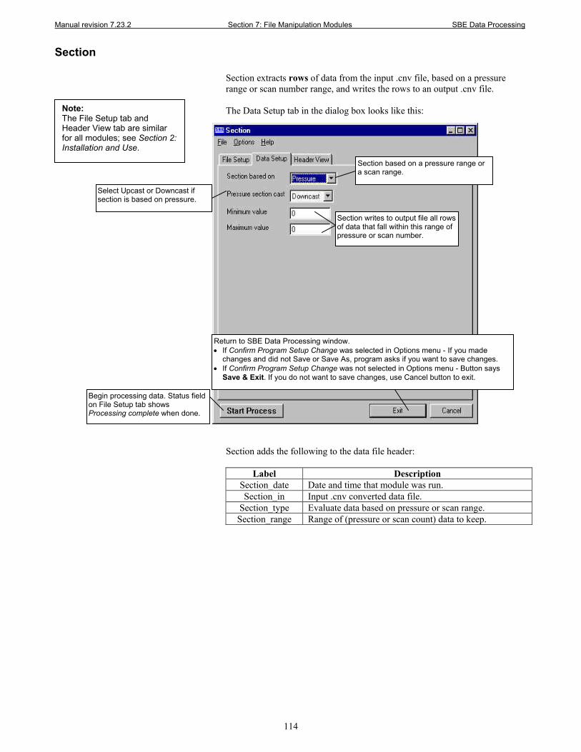
Manual revision 7.23.2 Section 7: File Manipulation Modules SBE Data Processing
114
Section Section extracts rows of data from the input .cnv file, based on a pressure range or scan number range, and writes the rows to an output .cnv file. The Data Setup tab in the dialog box looks like this:
Section adds the following to the data file header:
Label Description Section_date Date and time that module was run. Section_in Input .cnv converted data file.
Section_type Evaluate data based on pressure or scan range. Section_range Range of (pressure or scan count) data to keep.
Select Upcast or Downcast if section is based on pressure.
Section based on a pressure range or a scan range.
Section writes to output file all rows of data that fall within this range of pressure or scan number.
Return to SBE Data Processing window. • If Confirm Program Setup Change was selected in Options menu - If you made
changes and did not Save or Save As, program asks if you want to save changes. • If Confirm Program Setup Change was not selected in Options menu - Button says
Save & Exit. If you do not want to save changes, use Cancel button to exit.
Begin processing data. Status field on File Setup tab shows Processing complete when done.
Note: The File Setup tab and Header View tab are similar for all modules; see Section 2: Installation and Use.
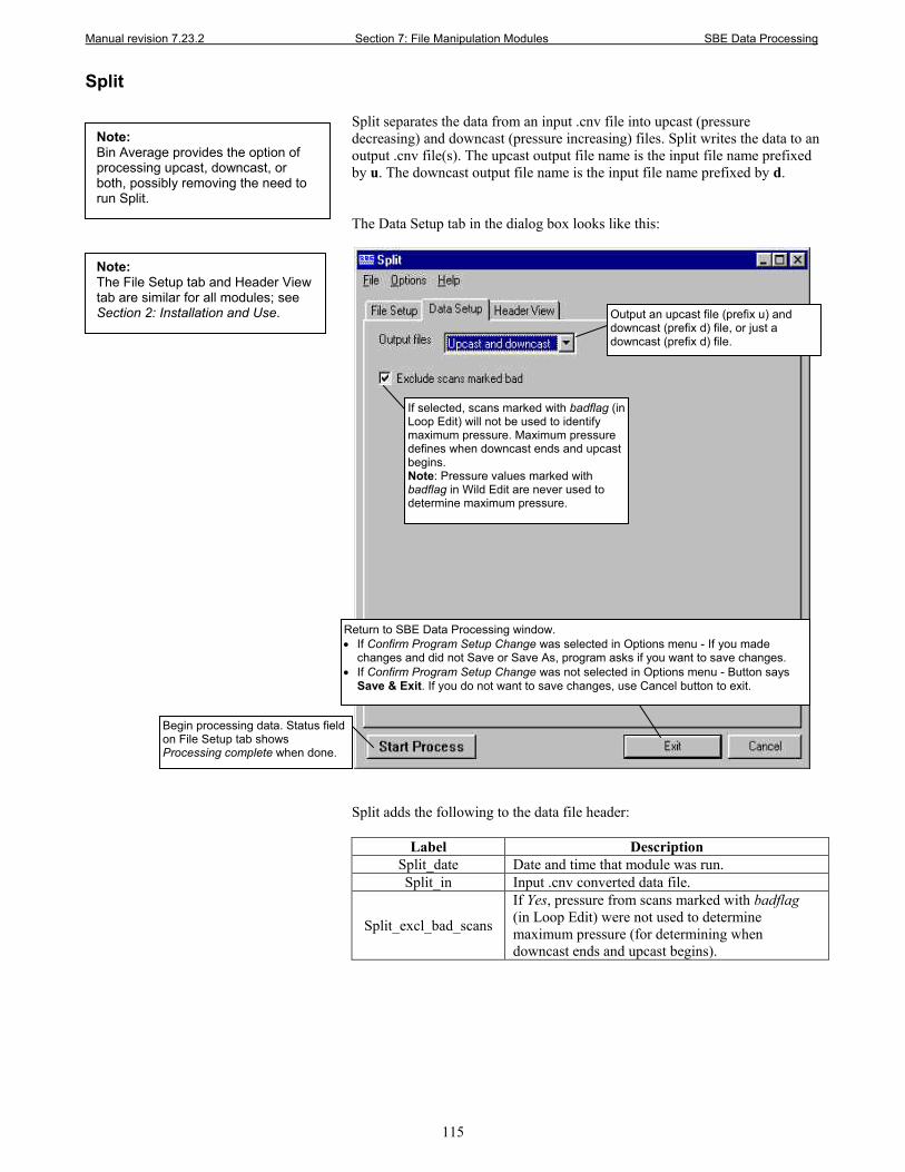
Manual revision 7.23.2 Section 7: File Manipulation Modules SBE Data Processing
115
Split Split separates the data from an input .cnv file into upcast (pressure decreasing) and downcast (pressure increasing) files. Split writes the data to an output .cnv file(s). The upcast output file name is the input file name prefixed by u. The downcast output file name is the input file name prefixed by d. The Data Setup tab in the dialog box looks like this:
Split adds the following to the data file header:
Label Description Split_date Date and time that module was run. Split_in Input .cnv converted data file.
Split_excl_bad_scans
If Yes, pressure from scans marked with badflag (in Loop Edit) were not used to determine maximum pressure (for determining when downcast ends and upcast begins).
Note: Bin Average provides the option of processing upcast, downcast, or both, possibly removing the need to run Split.
Output an upcast file (prefix u) and downcast (prefix d) file, or just a downcast (prefix d) file.
If selected, scans marked with badflag (in Loop Edit) will not be used to identify maximum pressure. Maximum pressure defines when downcast ends and upcast begins. Note: Pressure values marked with badflag in Wild Edit are never used to determine maximum pressure.
Return to SBE Data Processing window. • If Confirm Program Setup Change was selected in Options menu - If you made
changes and did not Save or Save As, program asks if you want to save changes. • If Confirm Program Setup Change was not selected in Options menu - Button says
Save & Exit. If you do not want to save changes, use Cancel button to exit.
Begin processing data. Status field on File Setup tab shows Processing complete when done.
Note: The File Setup tab and Header View tab are similar for all modules; see Section 2: Installation and Use.
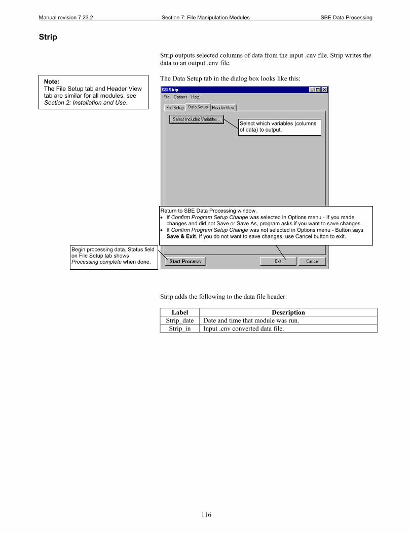
Manual revision 7.23.2 Section 7: File Manipulation Modules SBE Data Processing
116
Strip Strip outputs selected columns of data from the input .cnv file. Strip writes the data to an output .cnv file. The Data Setup tab in the dialog box looks like this:
Strip adds the following to the data file header:
Label Description Strip_date Date and time that module was run. Strip_in Input .cnv converted data file.
Select which variables (columns of data) to output.
Return to SBE Data Processing window. • If Confirm Program Setup Change was selected in Options menu - If you made
changes and did not Save or Save As, program asks if you want to save changes. • If Confirm Program Setup Change was not selected in Options menu - Button says
Save & Exit. If you do not want to save changes, use Cancel button to exit.
Begin processing data. Status field on File Setup tab shows Processing complete when done.
Note: The File Setup tab and Header View tab are similar for all modules; see Section 2: Installation and Use.
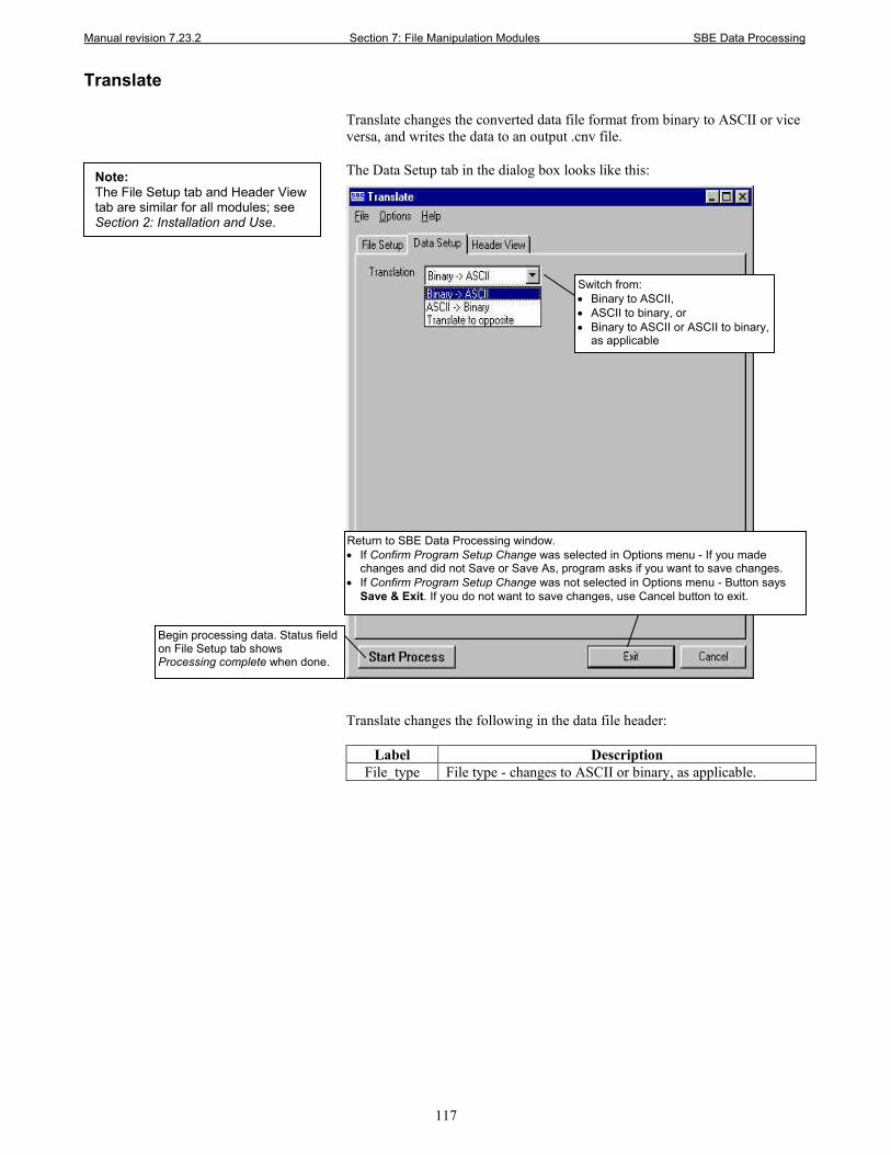
Manual revision 7.23.2 Section 7: File Manipulation Modules SBE Data Processing
117
Translate Translate changes the converted data file format from binary to ASCII or vice versa, and writes the data to an output .cnv file. The Data Setup tab in the dialog box looks like this:
Translate changes the following in the data file header:
Label Description File_type File type - changes to ASCII or binary, as applicable.
Switch from: • Binary to ASCII, • ASCII to binary, or • Binary to ASCII or ASCII to binary,
as applicable
Return to SBE Data Processing window. • If Confirm Program Setup Change was selected in Options menu - If you made
changes and did not Save or Save As, program asks if you want to save changes. • If Confirm Program Setup Change was not selected in Options menu - Button says
Save & Exit. If you do not want to save changes, use Cancel button to exit.
Begin processing data. Status field on File Setup tab shows Processing complete when done.
Note: The File Setup tab and Header View tab are similar for all modules; see Section 2: Installation and Use.
Manual revision 7.23.2 Section 8: Data Plotting Module – Sea Plot SBE Data Processing
118
Section 8: Data Plotting Module – Sea Plot
Sea Plot can be used to plot C, T, and P, as well as derived variables and data from auxiliary sensors, from any converted .cnv data file. Sea Plot can: • Plot up to 5 variables on one plot, with a single X axis and up to four
Y axes or a single Y axis and up to four X axes.
• Plot any variable on a linear or logarithmic scale (logarithmic scale not applicable to TS plots).
• Derive and plot derived salinity and/or derived density, if conductivity, temperature, and pressure data are in the input file. This allows you to skip running Derive if salinity and density are the only derived parameters you are interested in. Alternatively, you can calculate and plot derived salinity and/or derived density even if salinity and density are already in the input file; the values may differ because of processing steps performed on C, T, or P after Derive was run. Note that the calculations for derived salinity and derived density are based on EOS-80 equations (Practical Salinity). For TEOS-10 (Absolute Salinity), you must calculate the parameters in Derive TEOS-10 before plotting with Sea Plot.
• Plot time series data; the time scale selections include Julian Days, elapsed time in hours, minutes, or seconds, or date and time.
• Create contour plots, generating density (sigma-t or sigma-theta) or thermosteric anomaly contours on temperature-salinity (TS) plots.
• Process and plot multiple input files that contain the same variables and with the same setup parameters, each on their own plot, allowing the user to quickly switch the view from one file to the next.
• Process and plot multiple input files that contain the same variables on an overlay plot, allowing the user to view multiple sets of data at the same time. If desired, the user can offset each file on the plot to create a waterfall plot.
• Zoom in on plot features.
• Send plots to a printer, save plots to the clipboard for insertion in another program (such as Microsoft Word), or save plots as graphic files in bitmap, metafile, or JPEG format.
• Run in batch processing mode. See Appendix I: Command Line Options,
Command Line Operation, and Batch File Processing. The Sea Plot dialog box differs somewhat from the other SBE Data Processing modules. Each tab of the Sea Plot dialog box is described below, as well as options for viewing, printing, and saving a plot.
Notes: • Converted data (.cnv) files are
typically created in Data Conversion and manipulated in other SBE Data Processing modules. Sea Plot can plot data at any point after Data Conversion has been run. - For SBE 37 (firmware < 3.0), 39, 39-IM, and 48, a converted (.cnv) data file is created from an uploaded .asc file using the Convert button in Seaterm’s Toolbar. - For SBE 39plus, a converted (.cnv) data file is created from an uploaded .xml file using Convert .XML data file in SeatermV2’s Tools menu.
• Algorithms for calculation of derived parameters in Data Conversion, Derive, Sea Plot, SeaCalc III [EOS-80 (Practical Salinity) tab], and Seasave are identical, except as noted in Appendix V: Derived Parameter Formulas (EOS-80; Practical Salinity), and are based on EOS-80 equations.
• Calculation of Absolute Salinity and associated parameters (TEOS-10) is available in Derive TEOS-10 and SeaCalc III [TEOS-10 (Absolute Salinity) tab]. Once they are calculated in Derive TEOS-10, they can be plotted in Sea Plot. See Section 6: Data Processing Modules and Section 9: Miscellaneous Module – SeaCalc III.
Note: When plotting date and time, the following restrictions apply: • On the Plot Setup tab, select Single
X – Multiple Y or Single X – Multiple Y, Overlay for plot type
• On the X Axis tab, select Julian days or Elapsed time for the variable, and select Show as Date/Time.
• On the X Axis tab, do not select Reverse scale direction.
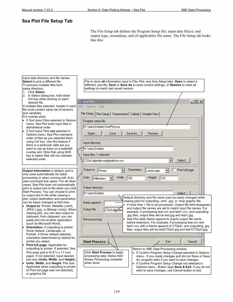
Manual revision 7.23.2 Section 8: Data Plotting Module – Sea Plot SBE Data Processing
119
Sea Plot File Setup Tab The File Setup tab defines the Program Setup file; input data file(s); and output type, orientation, and (if applicable) file name. The File Setup tab looks like this:
Output Information is default, and is only used automatically for batch processing or when running with Auto start command line option. For all other cases, Sea Plot does not automatically print or output plot to file when you click Start Process. You can choose to print or output plot to file while viewing a plot; output destination and parameters can be easily changed at that time. • Output to: Printer, Metafile (.wmf),
JPEG (.jpg), or Bitmap (.bmp). When viewing plot, you can also output to clipboard; from clipboard, you can paste plot into another application (such as Microsoft Word).
• Orientation: if outputting to printer. Driver default, Landscape, or Portrait. If Driver default selected, orientation determined by default for printer you select.
• Print full page: Applicable for outputting to printer. If selected, Sea Plot sizes plot to fit 81/2 x 11 inch paper. If not selected, input desired plot size (Units, Width, and Height).
• Units, Width, and Height: Plot size. Applicable when outputting to printer (if Print full page was not selected), or graphics file.
Return to SBE Data Processing window. • If Confirm Program Setup Change selected in Options
menu - If you made changes and did not Save or Save As, program asks if you want to save changes.
• If Confirm Program Setup Change not selected in Options menu - Button says Save & Exit. If you do not want to save changes, use Cancel button to exit.
Default directory and file name (can be easily changed while viewing plot) for outputting .wmf, .jpg, or .bmp graphic file. • If more than 1 file to be processed, Output file field disappears
and output file names are set to match input file names. For example, if processing test.cnv and test1.cnv, and outputting .jpg files, output files will be test.jpg and test1.jpg.
• Sea Plot adds Name append to (each) output file name, before extension. For example, if processing test.cnv and test1.cnv with a Name append of CTDpH, and outputting .jpg files, output files will be testCTDpH.jpg and test1CTDpH.jpg.
Click Start Process to begin processing data. Status field shows Processing complete when done.
Input data directory and file names. Select to pick a different file. To process multiple files from same directory: 1. Click Select. 2. In Select dialog box, hold down
Ctrl key while clicking on each desired file.
If multiple files selected, header in each file must contain same set of sensors and variables. For overlay plots: • If Sort Input Files selected in Options
menu: Sea Plot sorts input files in alphabetical order.
• If Sort Input Files not selected in Options menu: Sea Plot maintains order of files as you selected them using Ctrl key. Use this feature if there is a particular data set you want to use as base on a waterfall overlay plot. Note that using Shift key to select files will not maintain selected order.
File to store all information input in File, Plot, and Axis Setup tabs. Open to select a different .psa file, Save or Save As to save current settings, or Restore to reset all settings to match last saved version.
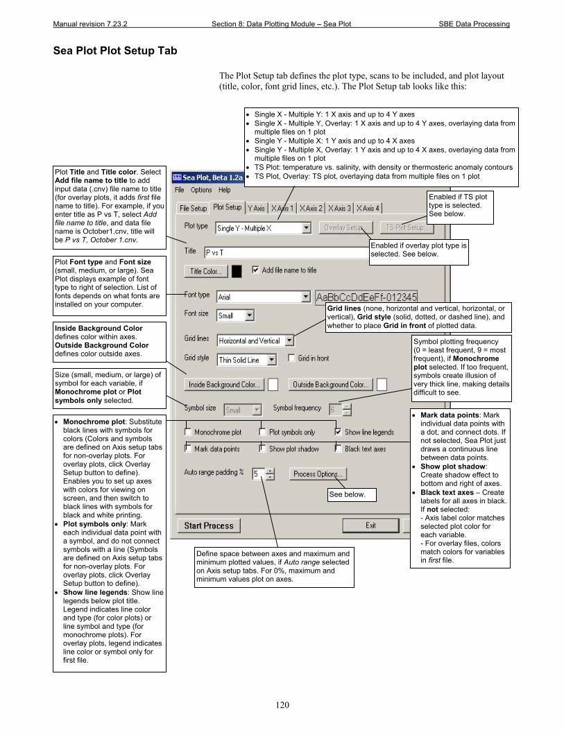
Manual revision 7.23.2 Section 8: Data Plotting Module – Sea Plot SBE Data Processing
120
Sea Plot Plot Setup Tab The Plot Setup tab defines the plot type, scans to be included, and plot layout (title, color, font grid lines, etc.). The Plot Setup tab looks like this:
• Single X - Multiple Y: 1 X axis and up to 4 Y axes • Single X - Multiple Y, Overlay: 1 X axis and up to 4 Y axes, overlaying data from
multiple files on 1 plot • Single Y - Multiple X: 1 Y axis and up to 4 X axes • Single Y - Multiple X, Overlay: 1 Y axis and up to 4 X axes, overlaying data from
multiple files on 1 plot • TS Plot: temperature vs. salinity, with density or thermosteric anomaly contours • TS Plot, Overlay: TS plot, overlaying data from multiple files on 1 plot Plot Title and Title color. Select
Add file name to title to add input data (.cnv) file name to title (for overlay plots, it adds first file name to title). For example, if you enter title as P vs T, select Add file name to title, and data file name is October1.cnv, title will be P vs T, October 1.cnv.
Plot Font type and Font size (small, medium, or large). Sea Plot displays example of font type to right of selection. List of fonts depends on what fonts are installed on your computer. Grid lines (none, horizontal and vertical, horizontal, or
vertical), Grid style (solid, dotted, or dashed line), and whether to place Grid in front of plotted data. Inside Background Color
defines color within axes. Outside Background Color defines color outside axes.
See below.
Size (small, medium, or large) of symbol for each variable, if Monochrome plot or Plot symbols only selected.
Symbol plotting frequency (0 = least frequent, 9 = most frequent), if Monochrome plot selected. If too frequent, symbols create illusion of very thick line, making details difficult to see.
• Monochrome plot: Substitute black lines with symbols for colors (Colors and symbols are defined on Axis setup tabs for non-overlay plots. For overlay plots, click Overlay Setup button to define). Enables you to set up axes with colors for viewing on screen, and then switch to black lines with symbols for black and white printing.
• Plot symbols only: Mark each individual data point with a symbol, and do not connect symbols with a line (Symbols are defined on Axis setup tabs for non-overlay plots. For overlay plots, click Overlay Setup button to define).
• Show line legends: Show line legends below plot title. Legend indicates line color and type (for color plots) or line symbol and type (for monochrome plots). For overlay plots, legend indicates line color or symbol only for first file.
Define space between axes and maximum and minimum plotted values, if Auto range selected on Axis setup tabs. For 0%, maximum and minimum values plot on axes.
• Mark data points: Mark individual data points with a dot, and connect dots. If not selected, Sea Plot just draws a continuous line between data points.
• Show plot shadow: Create shadow effect to bottom and right of axes.
• Black text axes – Create labels for all axes in black. If not selected: - Axis label color matches selected plot color for each variable. - For overlay files, colors match colors for variables in first file.
Enabled if overlay plot type is selected. See below.
Enabled if TS plot type is selected. See below.
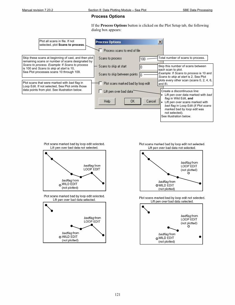
Manual revision 7.23.2 Section 8: Data Plotting Module – Sea Plot SBE Data Processing
121
Process Options If the Process Options button is clicked on the Plot Setup tab, the following dialog box appears:
Plot all scans in file. If not selected, plot Scans to process.
Total number of scans to process. Skip these scans at beginning of cast, and then plot remaining scans or number of scans designated by Scans to process. Example: If Scans to process is 100 and Scans to skip at start is 10, Sea Plot processes scans 10 through 109.
Skip this number of scans between each scan to plot. Example: If Scans to process is 10 and Scans to skip at start is 2, Sea Plot plots every other scan (scans 0, 2, 4, 6, and 8). Plot scans that were marked with bad flag in
Loop Edit. If not selected, Sea Plot omits those data points from plot. See illustration below. Create a discontinuous line:
• Lift pen over data marked with bad flag in Wild Edit, and
• Lift pen over scans marked with bad flag in Loop Edit (if Plot scans marked bad by loop edit was not selected).
See illustration below.
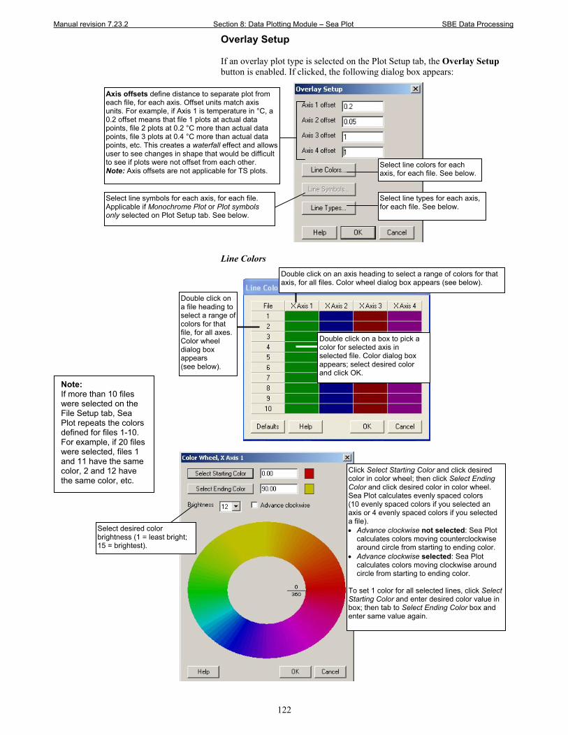
Manual revision 7.23.2 Section 8: Data Plotting Module – Sea Plot SBE Data Processing
122
Overlay Setup If an overlay plot type is selected on the Plot Setup tab, the Overlay Setup button is enabled. If clicked, the following dialog box appears:
Line Colors
Click Select Starting Color and click desired color in color wheel; then click Select Ending Color and click desired color in color wheel. Sea Plot calculates evenly spaced colors (10 evenly spaced colors if you selected an axis or 4 evenly spaced colors if you selected a file). • Advance clockwise not selected: Sea Plot
calculates colors moving counterclockwise around circle from starting to ending color.
• Advance clockwise selected: Sea Plot calculates colors moving clockwise around circle from starting to ending color.
To set 1 color for all selected lines, click Select Starting Color and enter desired color value in box; then tab to Select Ending Color box and enter same value again.
Select desired color brightness (1 = least bright; 15 = brightest).
Note: If more than 10 files were selected on the File Setup tab, Sea Plot repeats the colors defined for files 1-10. For example, if 20 files were selected, files 1 and 11 have the same color, 2 and 12 have the same color, etc.
Select line types for each axis, for each file. See below.
Select line colors for each axis, for each file. See below.
Axis offsets define distance to separate plot from each file, for each axis. Offset units match axis units. For example, if Axis 1 is temperature in °C, a 0.2 offset means that file 1 plots at actual data points, file 2 plots at 0.2 °C more than actual data points, file 3 plots at 0.4 °C more than actual data points, etc. This creates a waterfall effect and allows user to see changes in shape that would be difficult to see if plots were not offset from each other. Note: Axis offsets are not applicable for TS plots.
Select line symbols for each axis, for each file. Applicable if Monochrome Plot or Plot symbols only selected on Plot Setup tab. See below.
Double click on a file heading to select a range of colors for that file, for all axes. Color wheel dialog box appears (see below).
Double click on a box to pick a color for selected axis in selected file. Color dialog box appears; select desired color and click OK.
Double click on an axis heading to select a range of colors for that axis, for all files. Color wheel dialog box appears (see below).
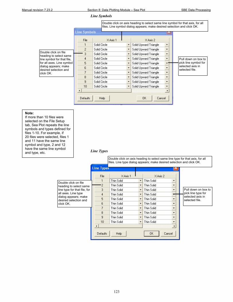
Manual revision 7.23.2 Section 8: Data Plotting Module – Sea Plot SBE Data Processing
123
Line Symbols
Line Types
Note: If more than 10 files were selected on the File Setup tab, Sea Plot repeats the line symbols and types defined for files 1-10. For example, if 20 files were selected, files 1 and 11 have the same line symbol and type, 2 and 12 have the same line symbol and type, etc.
Double click on axis heading to select same line symbol for that axis, for all files. Line symbol dialog appears; make desired selection and click OK.
Double click on file heading to select same line symbol for that file, for all axes. Line symbol dialog appears; make desired selection and click OK.
Pull down on box to pick line symbol for selected axis in selected file.
Double click on axis heading to select same line type for that axis, for all files. Line type dialog appears; make desired selection and click OK.
Double click on file heading to select same line type for that file, for all axes. Line type dialog appears; make desired selection and click OK.
Pull down on box to pick line type for selected axis in selected file.
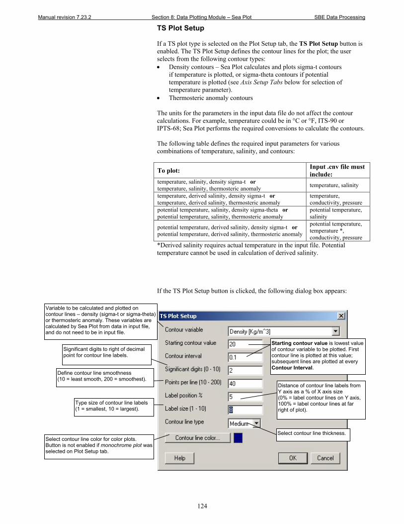
Manual revision 7.23.2 Section 8: Data Plotting Module – Sea Plot SBE Data Processing
124
TS Plot Setup If a TS plot type is selected on the Plot Setup tab, the TS Plot Setup button is enabled. The TS Plot Setup defines the contour lines for the plot; the user selects from the following contour types: • Density contours – Sea Plot calculates and plots sigma-t contours
if temperature is plotted, or sigma-theta contours if potential temperature is plotted (see Axis Setup Tabs below for selection of temperature parameter).
• Thermosteric anomaly contours The units for the parameters in the input data file do not affect the contour calculations. For example, temperature could be in °C or °F, ITS-90 or IPTS-68; Sea Plot performs the required conversions to calculate the contours. The following table defines the required input parameters for various combinations of temperature, salinity, and contours:
To plot: Input .cnv file must include:
temperature, salinity, density sigma-t or temperature, salinity, thermosteric anomaly temperature, salinity
temperature, derived salinity, density sigma-t or temperature, derived salinity, thermosteric anomaly
temperature, conductivity, pressure
potential temperature, salinity, density sigma-theta or potential temperature, salinity, thermosteric anomaly
potential temperature, salinity
potential temperature, derived salinity, density sigma-t or potential temperature, derived salinity, thermosteric anomaly
potential temperature, temperature *, conductivity, pressure
*Derived salinity requires actual temperature in the input file. Potential temperature cannot be used in calculation of derived salinity. If the TS Plot Setup button is clicked, the following dialog box appears:
Variable to be calculated and plotted on contour lines – density (sigma-t or sigma-theta) or thermosteric anomaly. These variables are calculated by Sea Plot from data in input file, and do not need to be in input file.
Significant digits to right of decimal point for contour line labels.
Starting contour value is lowest value of contour variable to be plotted. First contour line is plotted at this value; subsequent lines are plotted at every Contour Interval.
Distance of contour line labels from Y axis as a % of X axis size (0% = label contour lines on Y axis, 100% = label contour lines at far right of plot).
Type size of contour line labels (1 = smallest, 10 = largest).
Select contour line thickness.
Define contour line smoothness (10 = least smooth, 200 = smoothest).
Select contour line color for color plots. Button is not enabled if monochrome plot was selected on Plot Setup tab.
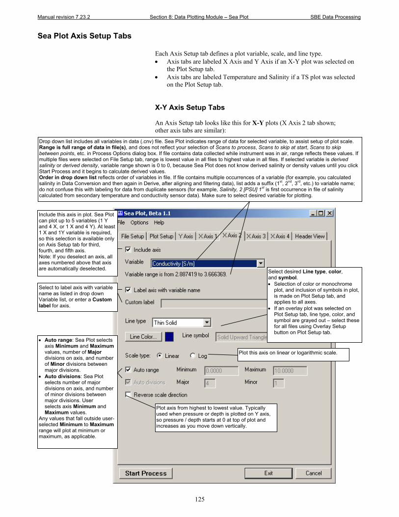
Manual revision 7.23.2 Section 8: Data Plotting Module – Sea Plot SBE Data Processing
125
Sea Plot Axis Setup Tabs Each Axis Setup tab defines a plot variable, scale, and line type. • Axis tabs are labeled X Axis and Y Axis if an X-Y plot was selected on
the Plot Setup tab. • Axis tabs are labeled Temperature and Salinity if a TS plot was selected
on the Plot Setup tab. X-Y Axis Setup Tabs An Axis Setup tab looks like this for X-Y plots (X Axis 2 tab shown; other axis tabs are similar):
Include this axis in plot. Sea Plot can plot up to 5 variables (1 Y and 4 X, or 1 X and 4 Y). At least 1 X and 1Y variable is required, so this selection is available only on Axis Setup tab for third, fourth, and fifth axis. Note: If you deselect an axis, all axes numbered above that axis are automatically deselected.
Drop down list includes all variables in data (.cnv) file. Sea Plot indicates range of data for selected variable, to assist setup of plot scale. Range is full range of data in file(s), and does not reflect your selection of Scans to process, Scans to skip at start, Scans to skip between points, etc. in Process Options dialog box. If file contains data collected while instrument was in air, range reflects these values. If multiple files were selected on File Setup tab, range is lowest value in all files to highest value in all files. If selected variable is derived salinity or derived density, variable range shown is 0 to 0, because Sea Plot does not know derived salinity or density values until you click Start Process and it begins to calculate derived values. Order in drop down list reflects order of variables in file. If file contains multiple occurrences of a variable (for example, you calculated salinity in Data Conversion and then again in Derive, after aligning and filtering data), list adds a suffix (1st, 2nd, 3rd, etc.) to variable name; do not confuse this with labeling for data from duplicate sensors (for example, Salinity, 2 [PSU] 1st is first occurrence in file of salinity calculated from secondary temperature and conductivity sensor data). Make sure to select desired variable for plotting.
• Auto range: Sea Plot selects axis Minimum and Maximum values, number of Major divisions on axis, and number of Minor divisions between major divisions.
• Auto divisions: Sea Plot selects number of major divisions on axis, and number of minor divisions between major divisions. User selects axis Minimum and Maximum values.
Any values that fall outside user-selected Minimum to Maximum range will plot at minimum or maximum, as applicable.
Select to label axis with variable name as listed in drop down Variable list, or enter a Custom label for axis.
Select desired Line type, color, and symbol. • Selection of color or monochrome
plot, and inclusion of symbols in plot, is made on Plot Setup tab, and applies to all axes.
• If an overlay plot was selected on Plot Setup tab, line type, color, and symbol are grayed out – select these for all files using Overlay Setup button on Plot Setup tab.
Plot axis from highest to lowest value. Typically used when pressure or depth is plotted on Y axis, so pressure / depth starts at 0 at top of plot and increases as you move down vertically.
Plot this axis on linear or logarithmic scale.
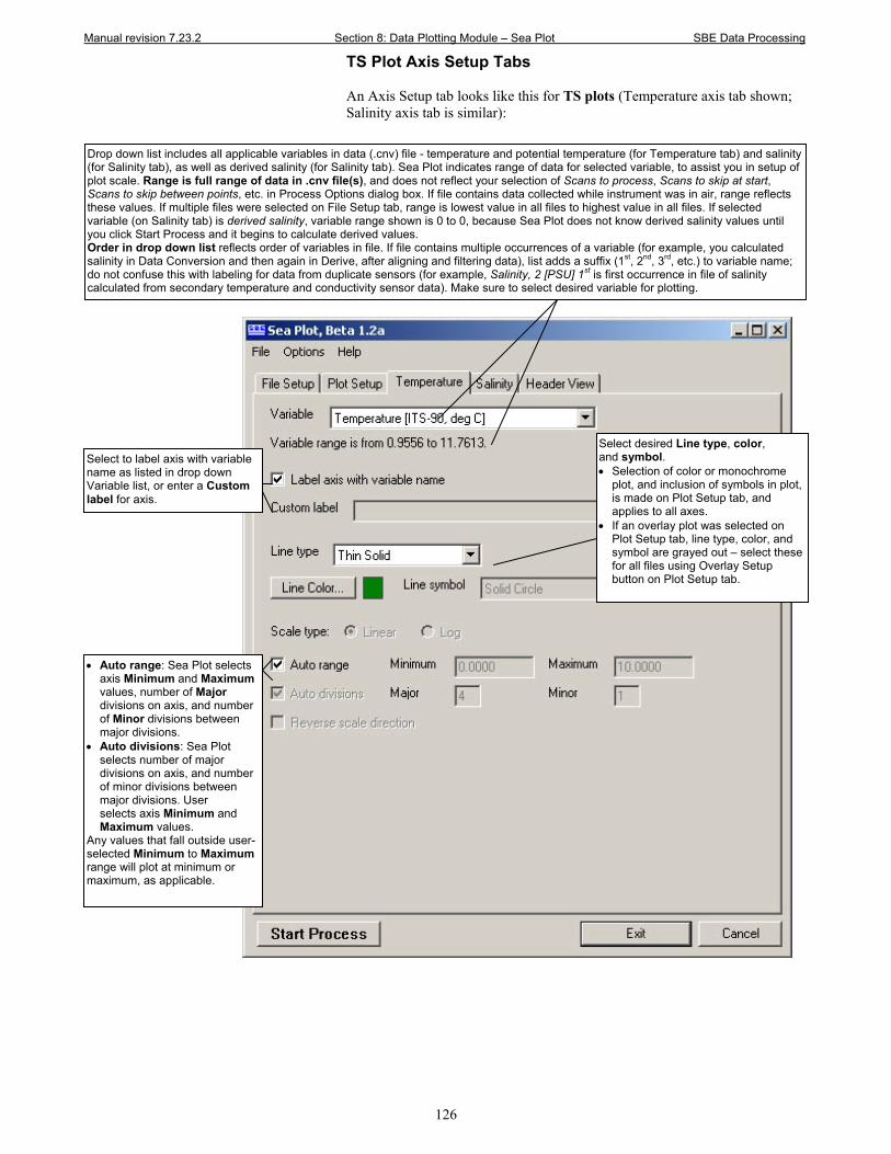
Manual revision 7.23.2 Section 8: Data Plotting Module – Sea Plot SBE Data Processing
126
TS Plot Axis Setup Tabs An Axis Setup tab looks like this for TS plots (Temperature axis tab shown; Salinity axis tab is similar):
Drop down list includes all applicable variables in data (.cnv) file - temperature and potential temperature (for Temperature tab) and salinity (for Salinity tab), as well as derived salinity (for Salinity tab). Sea Plot indicates range of data for selected variable, to assist you in setup of plot scale. Range is full range of data in .cnv file(s), and does not reflect your selection of Scans to process, Scans to skip at start, Scans to skip between points, etc. in Process Options dialog box. If file contains data collected while instrument was in air, range reflects these values. If multiple files were selected on File Setup tab, range is lowest value in all files to highest value in all files. If selected variable (on Salinity tab) is derived salinity, variable range shown is 0 to 0, because Sea Plot does not know derived salinity values until you click Start Process and it begins to calculate derived values. Order in drop down list reflects order of variables in file. If file contains multiple occurrences of a variable (for example, you calculated salinity in Data Conversion and then again in Derive, after aligning and filtering data), list adds a suffix (1st, 2nd, 3rd, etc.) to variable name; do not confuse this with labeling for data from duplicate sensors (for example, Salinity, 2 [PSU] 1st is first occurrence in file of salinity calculated from secondary temperature and conductivity sensor data). Make sure to select desired variable for plotting.
• Auto range: Sea Plot selects axis Minimum and Maximum values, number of Major divisions on axis, and number of Minor divisions between major divisions.
• Auto divisions: Sea Plot selects number of major divisions on axis, and number of minor divisions between major divisions. User selects axis Minimum and Maximum values.
Any values that fall outside user-selected Minimum to Maximum range will plot at minimum or maximum, as applicable.
Select to label axis with variable name as listed in drop down Variable list, or enter a Custom label for axis.
Select desired Line type, color, and symbol. • Selection of color or monochrome
plot, and inclusion of symbols in plot, is made on Plot Setup tab, and applies to all axes.
• If an overlay plot was selected on Plot Setup tab, line type, color, and symbol are grayed out – select these for all files using Overlay Setup button on Plot Setup tab.
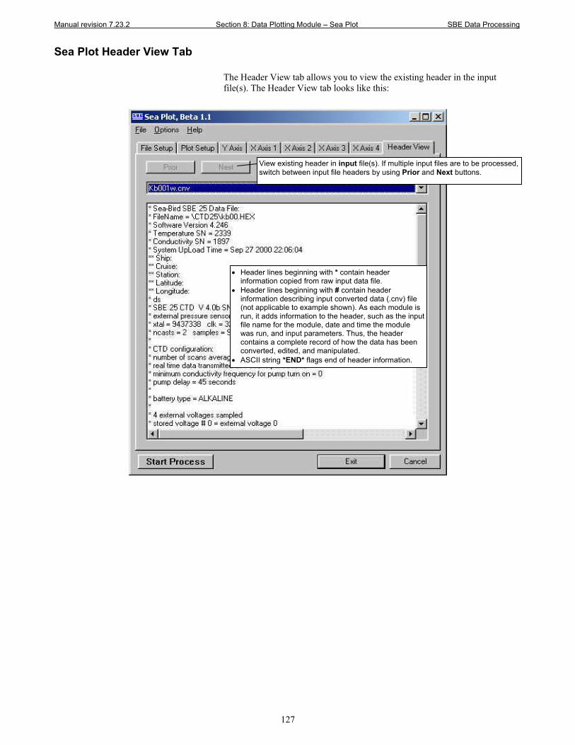
Manual revision 7.23.2 Section 8: Data Plotting Module – Sea Plot SBE Data Processing
127
Sea Plot Header View Tab The Header View tab allows you to view the existing header in the input file(s). The Header View tab looks like this:
View existing header in input file(s). If multiple input files are to be processed, switch between input file headers by using Prior and Next buttons.
• Header lines beginning with * contain header information copied from raw input data file.
• Header lines beginning with # contain header information describing input converted data (.cnv) file (not applicable to example shown). As each module is run, it adds information to the header, such as the input file name for the module, date and time the module was run, and input parameters. Thus, the header contains a complete record of how the data has been converted, edited, and manipulated.
• ASCII string *END* flags end of header information.
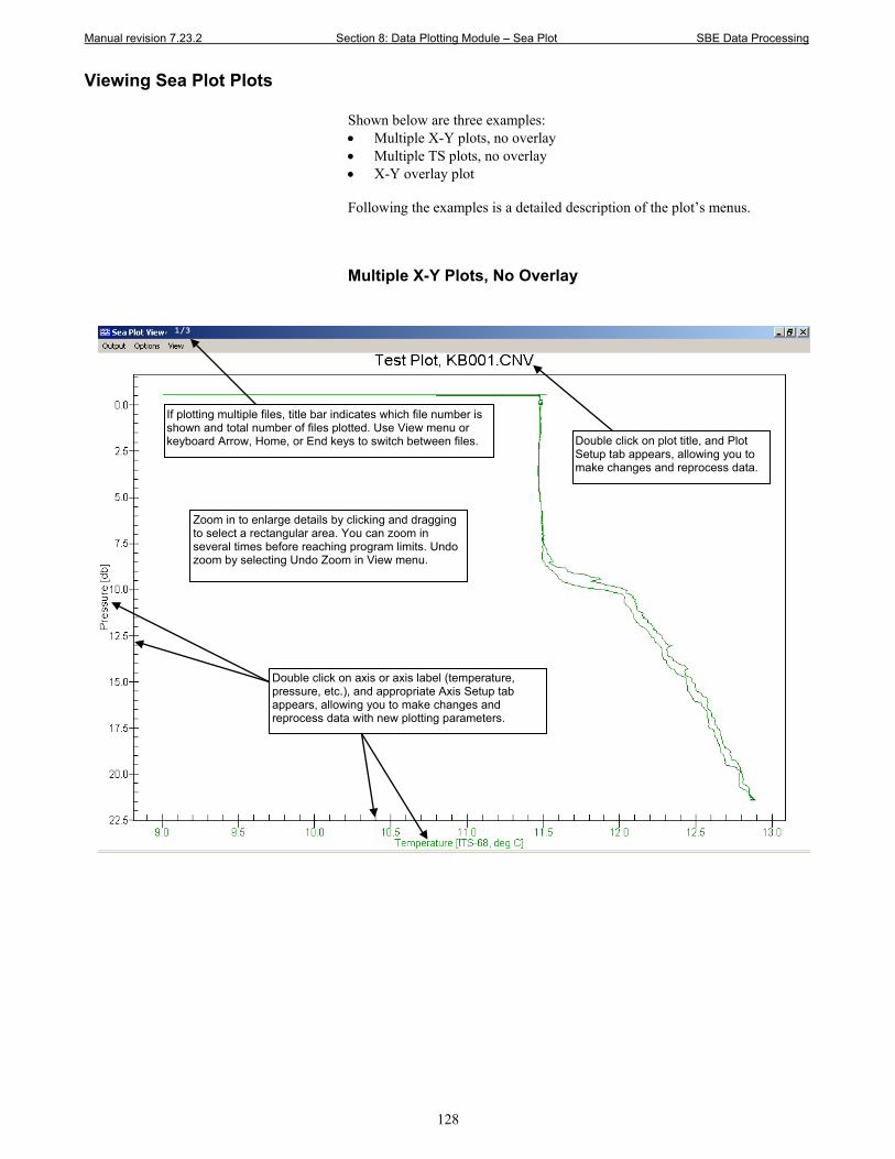
Manual revision 7.23.2 Section 8: Data Plotting Module – Sea Plot SBE Data Processing
128
Viewing Sea Plot Plots Shown below are three examples: • Multiple X-Y plots, no overlay • Multiple TS plots, no overlay • X-Y overlay plot Following the examples is a detailed description of the plot’s menus. Multiple X-Y Plots, No Overlay
Zoom in to enlarge details by clicking and dragging to select a rectangular area. You can zoom in several times before reaching program limits. Undo zoom by selecting Undo Zoom in View menu.
, 1/3
If plotting multiple files, title bar indicates which file number is shown and total number of files plotted. Use View menu or keyboard Arrow, Home, or End keys to switch between files.
Double click on axis or axis label (temperature, pressure, etc.), and appropriate Axis Setup tab appears, allowing you to make changes and reprocess data with new plotting parameters.
Double click on plot title, and Plot Setup tab appears, allowing you to make changes and reprocess data.
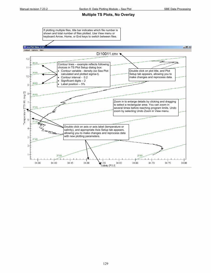
Manual revision 7.23.2 Section 8: Data Plotting Module – Sea Plot SBE Data Processing
129
Multiple TS Plots, No Overlay
Zoom in to enlarge details by clicking and dragging to select a rectangular area. You can zoom in several times before reaching program limits. Undo zoom by selecting Undo Zoom in View menu.
Contour lines – example reflects following choices in TS Plot Setup dialog box: • Contour variable - density (so Sea Plot
calculated and plotted sigma-t). • Contour interval - 0.2 • Significant digits – 2 • Label position – 5%
Double click on axis or axis label (temperature or salinity), and appropriate Axis Setup tab appears, allowing you to make changes and reprocess data with new plotting parameters.
Double click on plot title, and Plot Setup tab appears, allowing you to make changes and reprocess data.
If plotting multiple files, title bar indicates which file number is shown and total number of files plotted. Use View menu or keyboard Arrow, Home, or End keys to switch between files.
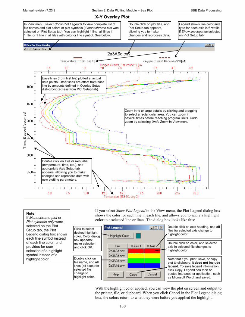
Manual revision 7.23.2 Section 8: Data Plotting Module – Sea Plot SBE Data Processing
130
X-Y Overlay Plot
If you select Show Plot Legend in the View menu, the Plot Legend dialog box shows the color for each line in each file, and allows you to apply a highlight color to a selected line or lines. The dialog box looks like this:
With the highlight color applied, you can view the plot on screen and output to the printer, file, or clipboard. When you click Cancel in the Plot Legend dialog box, the colors return to what they were before you applied the highlight.
Note: If Monochrome plot or Plot symbols only were selected on the Plot Setup tab, the Plot Legend dialog box shows each line symbol instead of each line color, and provides for user selection of a highlight symbol instead of a highlight color.
In View menu, select Show Plot Legends to view complete list of file names and plot colors or plot symbols (if monochrome plot was selected on Plot Setup tab). You can highlight 1 line, all lines in 1 file, or 1 line in all files with color or line symbol. See below.
Base lines (from first file) plotted at actual data points. Other lines are offset from base line by amounts defined in Overlay Setup dialog box (access from Plot Setup tab).
Zoom in to enlarge details by clicking and dragging to select a rectangular area. You can zoom in several times before reaching program limits. Undo zoom by selecting Undo Zoom in View menu.
Double click on axis or axis label (temperature, time, etc.), and appropriate Axis Setup tab appears, allowing you to make changes and reprocess data with new plotting parameters.
Double click on plot title, and Plot Setup tab appears, allowing you to make changes and reprocess data.
Legend shows line color and type for each axis in first file if Show line legends selected on Plot Setup tab.
Double click on axis heading, and all files for selected axis change to highlight color.
Double click on color, and selected axis in selected file changes to highlight color.
Double click on file name, and all lines (all axes) for selected file change to highlight color.
Click to select desired highlight color. Color dialog box appears; make selection and click OK.
Note that if you print, save, or copy plot to clipboard, it does not include legend. To save legend information, click Copy. Legend can then be pasted into another application, such as Microsoft Word, and saved.
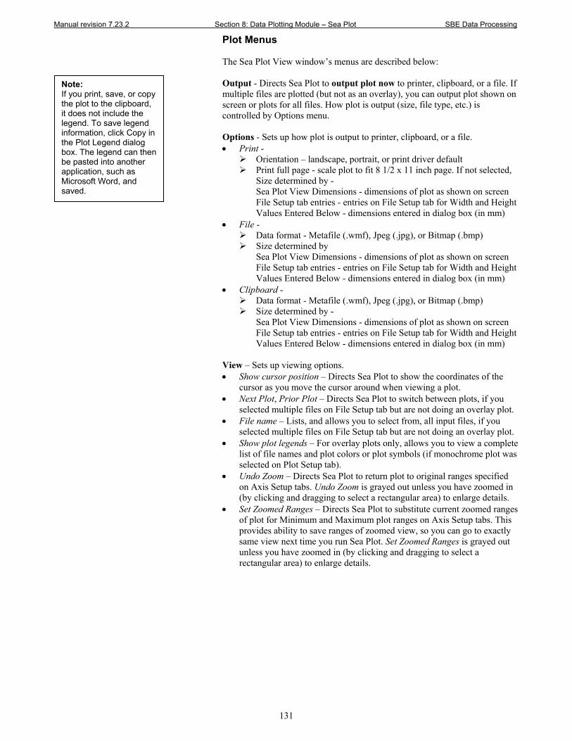
Manual revision 7.23.2 Section 8: Data Plotting Module – Sea Plot SBE Data Processing
131
Plot Menus The Sea Plot View window’s menus are described below: Output - Directs Sea Plot to output plot now to printer, clipboard, or a file. If multiple files are plotted (but not as an overlay), you can output plot shown on screen or plots for all files. How plot is output (size, file type, etc.) is controlled by Options menu. Options - Sets up how plot is output to printer, clipboard, or a file. • Print -
Orientation – landscape, portrait, or print driver default Print full page - scale plot to fit 8 1/2 x 11 inch page. If not selected,
Size determined by - Sea Plot View Dimensions - dimensions of plot as shown on screen File Setup tab entries - entries on File Setup tab for Width and Height Values Entered Below - dimensions entered in dialog box (in mm)
• File - Data format - Metafile (.wmf), Jpeg (.jpg), or Bitmap (.bmp) Size determined by
Sea Plot View Dimensions - dimensions of plot as shown on screen File Setup tab entries - entries on File Setup tab for Width and Height Values Entered Below - dimensions entered in dialog box (in mm)
• Clipboard - Data format - Metafile (.wmf), Jpeg (.jpg), or Bitmap (.bmp) Size determined by -
Sea Plot View Dimensions - dimensions of plot as shown on screen File Setup tab entries - entries on File Setup tab for Width and Height Values Entered Below - dimensions entered in dialog box (in mm)
View – Sets up viewing options. • Show cursor position – Directs Sea Plot to show the coordinates of the
cursor as you move the cursor around when viewing a plot. • Next Plot, Prior Plot – Directs Sea Plot to switch between plots, if you
selected multiple files on File Setup tab but are not doing an overlay plot. • File name – Lists, and allows you to select from, all input files, if you
selected multiple files on File Setup tab but are not doing an overlay plot. • Show plot legends – For overlay plots only, allows you to view a complete
list of file names and plot colors or plot symbols (if monochrome plot was selected on Plot Setup tab).
• Undo Zoom – Directs Sea Plot to return plot to original ranges specified on Axis Setup tabs. Undo Zoom is grayed out unless you have zoomed in (by clicking and dragging to select a rectangular area) to enlarge details.
• Set Zoomed Ranges – Directs Sea Plot to substitute current zoomed ranges of plot for Minimum and Maximum plot ranges on Axis Setup tabs. This provides ability to save ranges of zoomed view, so you can go to exactly same view next time you run Sea Plot. Set Zoomed Ranges is grayed out unless you have zoomed in (by clicking and dragging to select a rectangular area) to enlarge details.
Note: If you print, save, or copy the plot to the clipboard, it does not include the legend. To save legend information, click Copy in the Plot Legend dialog box. The legend can then be pasted into another application, such as Microsoft Word, and saved.
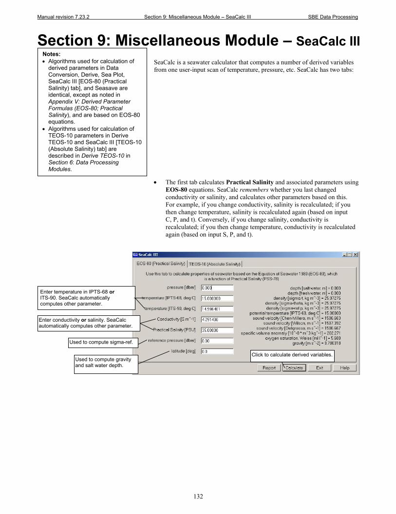
Manual revision 7.23.2 Section 9: Miscellaneous Module – SeaCalc III SBE Data Processing
132
Section 9: Miscellaneous Module – SeaCalc III
SeaCalc is a seawater calculator that computes a number of derived variables from one user-input scan of temperature, pressure, etc. SeaCalc has two tabs: • The first tab calculates Practical Salinity and associated parameters using
EOS-80 equations. SeaCalc remembers whether you last changed conductivity or salinity, and calculates other parameters based on this. For example, if you change conductivity, salinity is recalculated; if you then change temperature, salinity is recalculated again (based on input C, P, and t). Conversely, if you change salinity, conductivity is recalculated; if you then change temperature, conductivity is recalculated again (based on input S, P, and t).
Notes: • Algorithms used for calculation of
derived parameters in Data Conversion, Derive, Sea Plot, SeaCalc III [EOS-80 (Practical Salinity) tab], and Seasave are identical, except as noted in Appendix V: Derived Parameter Formulas (EOS-80; Practical Salinity), and are based on EOS-80 equations.
• Algorithms used for calculation of TEOS-10 parameters in Derive TEOS-10 and SeaCalc III [TEOS-10 (Absolute Salinity) tab] are described in Derive TEOS-10 in Section 6: Data Processing Modules.
Enter temperature in IPTS-68 or ITS-90. SeaCalc automatically computes other parameter.
Enter conductivity or salinity. SeaCalc automatically computes other parameter.
Click to calculate derived variables.
Used to compute sigma-ref.
Used to compute gravity and salt water depth.
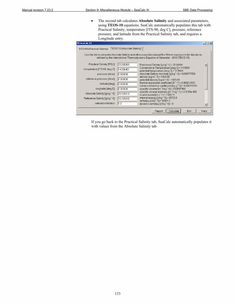
Manual revision 7.23.2 Section 9: Miscellaneous Module – SeaCalc III SBE Data Processing
133
• The second tab calculates Absolute Salinity and associated parameters,
using TEOS-10 equations. SeaCalc automatically populates this tab with Practical Salinity, temperature [ITS-90, deg C], pressure, reference pressure, and latitude from the Practical Salinity tab, and requires a Longitude entry.
If you go back to the Practical Salinity tab, SeaCalc automatically populates it with values from the Absolute Salinity tab.
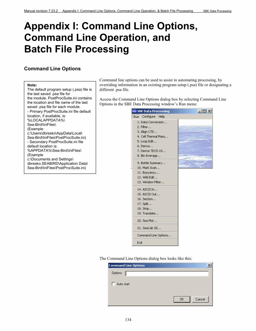
Manual revision 7.23.2 Appendix I: Command Line Options, Command Line Operation, & Batch File Processing SBE Data Processing
134
Appendix I: Command Line Options, Command Line Operation, and Batch File Processing
Command Line Options Command line options can be used to assist in automating processing, by overriding information in an existing program setup (.psa) file or designating a different .psa file. Access the Command Line Options dialog box by selecting Command Line Options in the SBE Data Processing window’s Run menu:
The Command Line Options dialog box looks like this:
Note: The default program setup (.psa) file is the last saved .psa file for the module. PostProcSuite.ini contains the location and file name of the last saved .psa file for each module. - Primary PostProcSuite.ini file default location, if available, is: %LOCALAPPDATA%\ Sea-Bird\IniFiles\ (Example c:\Users\dbresko\AppData\Local\ Sea-Bird\IniFiles\PostProcSuite.ini) - Secondary PostProcSuite.ini file default location is: %APPDATA%\Sea-Bird\IniFiles\ (Example c:\Documents and Settings\ dbresko.SEABIRD\Application Data\ Sea-Bird\IniFiles\PostProcSuite.ini)
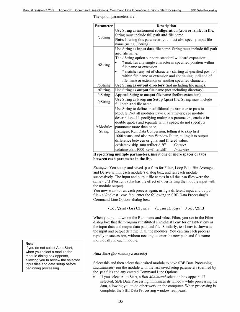
Manual revision 7.23.2 Appendix I: Command Line Options, Command Line Operation, & Batch File Processing SBE Data Processing
135
The option parameters are: Parameter Description
/cString
Use String as instrument configuration (.con or .xmlcon) file. String must include full path and file name. Note: If using this parameter, you must also specify input file name (using /iString).
/iString
Use String as input data file name. String must include full path and file name. The /iString option supports standard wildcard expansion: • ? matches any single character in specified position within
file name or extension. • * matches any set of characters starting at specified position
within file name or extension and continuing until end of file name or extension or another specified character.
/oString Use String as output directory (not including file name). /fString Use String as output file name (not including directory). /aString Append String to output file name (before extension).
/pString Use String as Program Setup (.psa) file. String must include full path and file name.
/xModule: String
Use String to define an additional parameter to pass to Module. Not all modules have x parameters; see module descriptions. If specifying multiple x parameters, enclose in double quotes and separate with a space; do not specify x parameter more than once. Example: Run Data Conversion, telling it to skip first 1000 scans, and also run Window Filter, telling it to output difference between original and filtered value: /x“datcnv:skip1000 wfilter:diff” Correct /xdatcnv:skip1000 /xwfilter:diff Incorrect
If specifying multiple parameters, insert one or more spaces or tabs between each parameter in the list. Example: You set up and saved .psa files for Filter, Loop Edit, Bin Average, and Derive within each module’s dialog box, and ran each module successively. The input and output file names in all the .psa files were the same - c:\1st\test.cnv (this has the effect of overwriting the module input with the module output). You now want to run each process again, using a different input and output file - c:\2nd\test1.cnv. You enter the following in SBE Data Processing’s Command Line Options dialog box:
/ic:\2nd\test1.cnv /ftest1.cnv /oc:\2nd
When you pull down on the Run menu and select Filter, you see in the Filter dialog box that the program substituted c:\2nd\test1.cnv for c:\1st\test.cnv as the input data and output data path and file. Similarly, test1.cnv is shown as the input and output data file in all the modules. You can run each process rapidly in succession, without needing to enter the new path and file name individually in each module. Auto Start (for running a module) Select this and then select the desired module to have SBE Data Processing automatically run the module with the last saved setup parameters (defined by the .psa file) and any entered Command Line Options. • If you select Auto Start, a Run Minimized selection box appears. If
selected, SBE Data Processing minimizes its window while processing the data, allowing you to do other work on the computer. When processing is complete, the SBE Data Processing window reappears.
Note: If you do not select Auto Start, when you select a module the module dialog box appears, allowing you to review the selected input files and data setup before beginning processing.
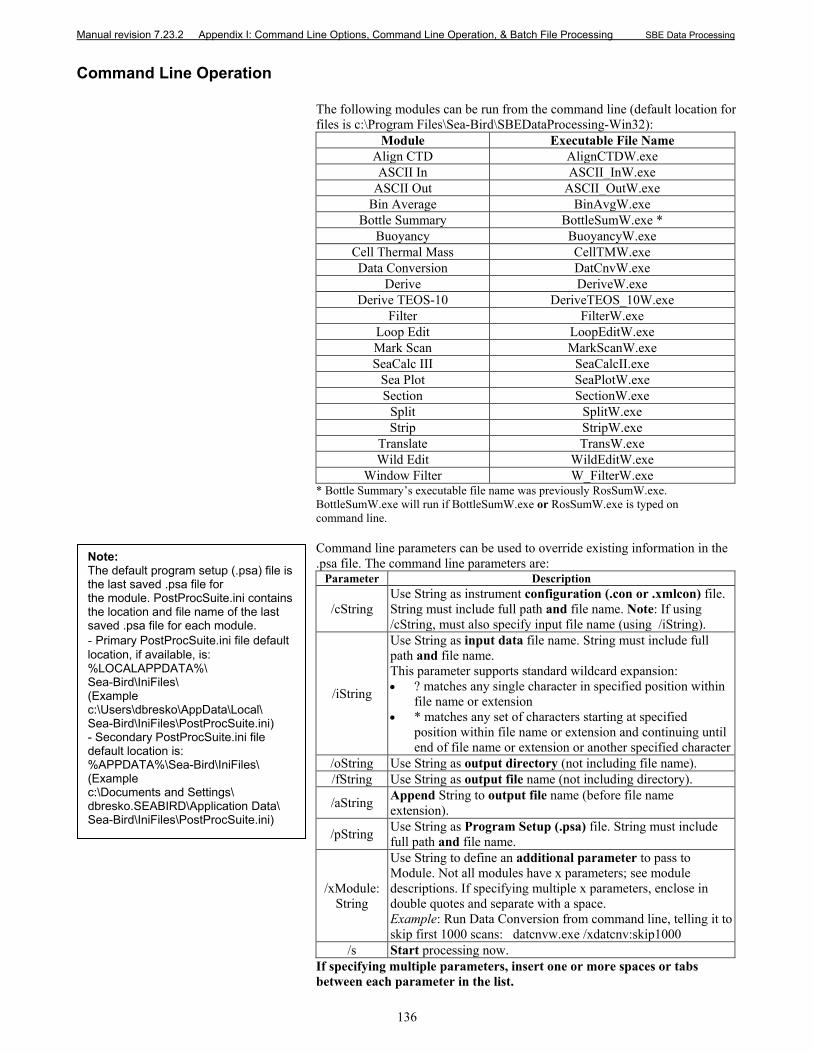
Manual revision 7.23.2 Appendix I: Command Line Options, Command Line Operation, & Batch File Processing SBE Data Processing
136
Command Line Operation The following modules can be run from the command line (default location for files is c:\Program Files\Sea-Bird\SBEDataProcessing-Win32):
Module Executable File Name Align CTD AlignCTDW.exe ASCII In ASCII_InW.exe
ASCII Out ASCII_OutW.exe Bin Average BinAvgW.exe
Bottle Summary BottleSumW.exe * Buoyancy BuoyancyW.exe
Cell Thermal Mass CellTMW.exe Data Conversion DatCnvW.exe
Derive DeriveW.exe Derive TEOS-10 DeriveTEOS_10W.exe
Filter FilterW.exe Loop Edit LoopEditW.exe Mark Scan MarkScanW.exe SeaCalc III SeaCalcII.exe
Sea Plot SeaPlotW.exe Section SectionW.exe
Split SplitW.exe Strip StripW.exe
Translate TransW.exe Wild Edit WildEditW.exe
Window Filter W_FilterW.exe * Bottle Summary’s executable file name was previously RosSumW.exe. BottleSumW.exe will run if BottleSumW.exe or RosSumW.exe is typed on command line. Command line parameters can be used to override existing information in the .psa file. The command line parameters are:
Parameter Description
/cString Use String as instrument configuration (.con or .xmlcon) file. String must include full path and file name. Note: If using /cString, must also specify input file name (using /iString).
/iString
Use String as input data file name. String must include full path and file name. This parameter supports standard wildcard expansion: • ? matches any single character in specified position within
file name or extension • * matches any set of characters starting at specified
position within file name or extension and continuing until end of file name or extension or another specified character
/oString Use String as output directory (not including file name). /fString Use String as output file name (not including directory).
/aString Append String to output file name (before file name extension).
/pString Use String as Program Setup (.psa) file. String must include full path and file name.
/xModule: String
Use String to define an additional parameter to pass to Module. Not all modules have x parameters; see module descriptions. If specifying multiple x parameters, enclose in double quotes and separate with a space. Example: Run Data Conversion from command line, telling it to skip first 1000 scans: datcnvw.exe /xdatcnv:skip1000
/s Start processing now. If specifying multiple parameters, insert one or more spaces or tabs between each parameter in the list.
Note: The default program setup (.psa) file is the last saved .psa file for the module. PostProcSuite.ini contains the location and file name of the last saved .psa file for each module. - Primary PostProcSuite.ini file default location, if available, is: %LOCALAPPDATA%\ Sea-Bird\IniFiles\ (Example c:\Users\dbresko\AppData\Local\ Sea-Bird\IniFiles\PostProcSuite.ini) - Secondary PostProcSuite.ini file default location is: %APPDATA%\Sea-Bird\IniFiles\ (Example c:\Documents and Settings\ dbresko.SEABIRD\Application Data\ Sea-Bird\IniFiles\PostProcSuite.ini)
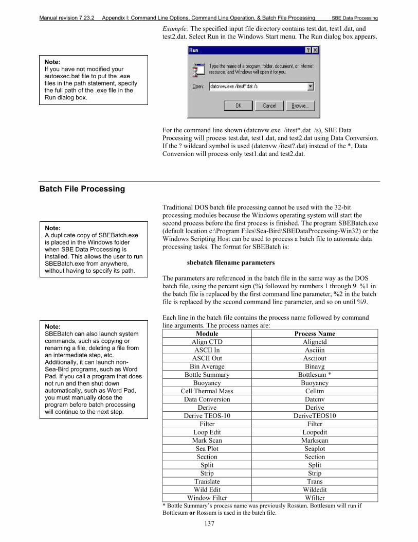
Manual revision 7.23.2 Appendix I: Command Line Options, Command Line Operation, & Batch File Processing SBE Data Processing
137
Example: The specified input file directory contains test.dat, test1.dat, and test2.dat. Select Run in the Windows Start menu. The Run dialog box appears.
For the command line shown (datcnvw.exe /itest*.dat /s), SBE Data Processing will process test.dat, test1.dat, and test2.dat using Data Conversion. If the ? wildcard symbol is used (datcnvw /itest?.dat) instead of the *, Data Conversion will process only test1.dat and test2.dat.
Batch File Processing Traditional DOS batch file processing cannot be used with the 32-bit processing modules because the Windows operating system will start the second process before the first process is finished. The program SBEBatch.exe (default location c:\Program Files\Sea-Bird\SBEDataProcessing-Win32) or the Windows Scripting Host can be used to process a batch file to automate data processing tasks. The format for SBEBatch is:
sbebatch filename parameters The parameters are referenced in the batch file in the same way as the DOS batch file, using the percent sign (%) followed by numbers 1 through 9. %1 in the batch file is replaced by the first command line parameter, %2 in the batch file is replaced by the second command line parameter, and so on until %9. Each line in the batch file contains the process name followed by command line arguments. The process names are:
Module Process Name Align CTD Alignctd ASCII In Asciiin
ASCII Out Asciiout Bin Average Binavg
Bottle Summary Bottlesum * Buoyancy Buoyancy
Cell Thermal Mass Celltm Data Conversion Datcnv
Derive Derive Derive TEOS-10 DeriveTEOS10
Filter Filter Loop Edit Loopedit Mark Scan Markscan
Sea Plot Seaplot Section Section
Split Split Strip Strip
Translate Trans Wild Edit Wildedit
Window Filter Wfilter * Bottle Summary’s process name was previously Rossum. Bottlesum will run if Bottlesum or Rossum is used in the batch file.
Note: If you have not modified your autoexec.bat file to put the .exe files in the path statement, specify the full path of the .exe file in the Run dialog box.
Note: A duplicate copy of SBEBatch.exe is placed in the Windows folder when SBE Data Processing is installed. This allows the user to run SBEBatch.exe from anywhere, without having to specify its path.
Note: SBEBatch can also launch system commands, such as copying or renaming a file, deleting a file from an intermediate step, etc. Additionally, it can launch non- Sea-Bird programs, such as Word Pad. If you call a program that does not run and then shut down automatically, such as Word Pad, you must manually close the program before batch processing will continue to the next step.
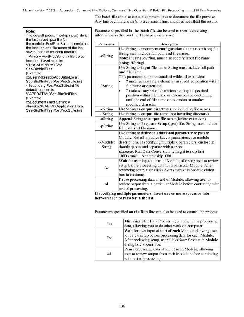
Manual revision 7.23.2 Appendix I: Command Line Options, Command Line Operation, & Batch File Processing SBE Data Processing
138
The batch file can also contain comment lines to document the file purpose. Any line beginning with @ is a comment line, and does not affect the results. Parameters specified in the batch file can be used to override existing information in the .psa file. These parameters are:
Parameter Description
/cString
Use String as instrument configuration (.con or .xmlcon) file. String must include full path and file name. Note: If using /cString, must also specify input file name (using /iString).
/iString
Use String as input file name. String must include full path and file name. This parameter supports standard wildcard expansion: • ? matches any single character in specified position within
file name or extension • * matches any set of characters starting at specified
position within file name or extension and continuing until the end of file name or extension or another specified character
/oString Use String as output directory (not including file name). /fString Use String as output file name (not including directory). /aString Append String to output file name (before extension).
/pString Use String as Program Setup (.psa) file. String must include full path and file name.
/xModule: String
Use String to define an additional parameter to pass to Module. Not all modules have x parameters; see module descriptions. If specifying multiple x parameters, enclose in double quotes and separate with a space. Example: Run Data Conversion, telling it to skip first 1000 scans: /xdatcnv:skip1000
/w
Wait for user input at start of Module, allowing user to review setup before processing data for a particular Module. After reviewing setup, user clicks Start Process in Module dialog box to continue.
/d Pause processing data at end of Module, allowing user to review output from a particular Module before continuing with rest of processing.
If specifying multiple parameters, insert one or more spaces or tabs between each parameter in the list. Parameters specified on the Run line can also be used to control the process:
#m Minimize SBE Data Processing window while processing data, allowing you to do other work on computer.
#w
Wait for user input at start of each Module, allowing user to review setup before processing data for each Module. After reviewing setup, user clicks Start Process in Module dialog box to continue.
#d Pause processing data at end of each Module, allowing user to review output from each Module before continuing with rest of processing.
Note: The default program setup (.psa) file is the last saved .psa file for the module. PostProcSuite.ini contains the location and file name of the last saved .psa file for each module. - Primary PostProcSuite.ini file default location, if available, is: %LOCALAPPDATA%\ Sea-Bird\IniFiles\ (Example c:\Users\dbresko\AppData\Local\ Sea-Bird\IniFiles\PostProcSuite.ini) - Secondary PostProcSuite.ini file default location is: %APPDATA%\Sea-Bird\IniFiles\ (Example c:\Documents and Settings\ dbresko.SEABIRD\Application Data\ Sea-Bird\IniFiles\PostProcSuite.ini)
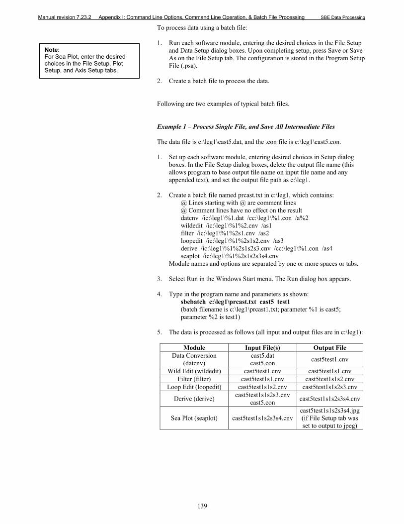
Manual revision 7.23.2 Appendix I: Command Line Options, Command Line Operation, & Batch File Processing SBE Data Processing
139
To process data using a batch file: 1. Run each software module, entering the desired choices in the File Setup
and Data Setup dialog boxes. Upon completing setup, press Save or Save As on the File Setup tab. The configuration is stored in the Program Setup File (.psa).
2. Create a batch file to process the data. Following are two examples of typical batch files. Example 1 – Process Single File, and Save All Intermediate Files The data file is c:\leg1\cast5.dat, and the .con file is c:\leg1\cast5.con. 1. Set up each software module, entering desired choices in Setup dialog
boxes. In the File Setup dialog boxes, delete the output file name (this allows program to base output file name on input file name and any appended text), and set the output file path as c:\leg1.
2. Create a batch file named prcast.txt in c:\leg1, which contains:
@ Lines starting with @ are comment lines @ Comment lines have no effect on the result datcnv /ic:\leg1\%1.dat /cc:\leg1\%1.con /a%2 wildedit /ic:\leg1\%1%2.cnv /as1 filter /ic:\leg1\%1%2s1.cnv /as2 loopedit /ic:\leg1\%1%2s1s2.cnv /as3 derive /ic:\leg1\%1%2s1s2s3.cnv /cc:\leg1\%1.con /as4 seaplot /ic:\leg1\%1%2s1s2s3s4.cnv
Module names and options are separated by one or more spaces or tabs.
3. Select Run in the Windows Start menu. The Run dialog box appears. 4. Type in the program name and parameters as shown:
sbebatch c:\leg1\prcast.txt cast5 test1 (batch filename is c:\leg1\prcast1.txt; parameter %1 is cast5; parameter %2 is test1)
5. The data is processed as follows (all input and output files are in c:\leg1):
Module Input File(s) Output File Data Conversion
(datcnv) cast5.dat cast5.con cast5test1.cnv
Wild Edit (wildedit) cast5test1.cnv cast5test1s1.cnv Filter (filter) cast5test1s1.cnv cast5test1s1s2.cnv
Loop Edit (loopedit) cast5test1s1s2.cnv cast5test1s1s2s3.cnv
Derive (derive) cast5test1s1s2s3.cnv cast5.con cast5test1s1s2s3s4.cnv
Sea Plot (seaplot) cast5test1s1s2s3s4.cnv cast5test1s1s2s3s4.jpg (if File Setup tab was set to output to jpeg)
Note: For Sea Plot, enter the desired choices in the File Setup, Plot Setup, and Axis Setup tabs.
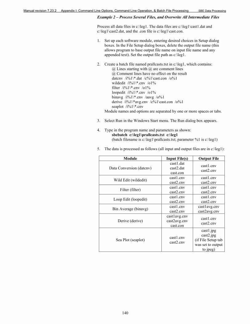
Manual revision 7.23.2 Appendix I: Command Line Options, Command Line Operation, & Batch File Processing SBE Data Processing
140
Example 2 – Process Several Files, and Overwrite All Intermediate Files Process all data files in c:\leg1. The data files are c:\leg1\cast1.dat and c:\leg1\cast2.dat, and the .con file is c:\leg1\cast.con. 1. Set up each software module, entering desired choices in Setup dialog
boxes. In the File Setup dialog boxes, delete the output file name (this allows program to base output file name on input file name and any appended text). Set the output file path as c:\leg1.
2. Create a batch file named prallcasts.txt in c:\leg1, which contains:
@ Lines starting with @ are comment lines @ Comment lines have no effect on the result datcnv /i%1\*.dat /c%1\cast.con /o%1 wildedit /i%1\*.cnv /o1% filter /i%1\*.cnv /o1% loopedit /i%1\*.cnv /o1% binavg /i%1\*.cnv /aavg /o%1 derive /i%1\*avg.cnv /c%1\cast.con /o%1 seaplot /i%1\*.cnv
Module names and options are separated by one or more spaces or tabs.
3. Select Run in the Windows Start menu. The Run dialog box appears. 4. Type in the program name and parameters as shown:
sbebatch c:\leg1\prallcasts.txt c:\leg1 (batch filename is c:\leg1\prallcasts.txt; parameter %1 is c:\leg1)
5. The data is processed as follows (all input and output files are in c:\leg1):
Module Input File(s) Output File
Data Conversion (datcnv) cast1.dat cast2.dat cast.con
cast1.cnv cast2.cnv
Wild Edit (wildedit) cast1.cnv cast2.cnv
cast1.cnv cast2.cnv
Filter (filter) cast1.cnv cast2.cnv
cast1.cnv cast2.cnv
Loop Edit (loopedit) cast1.cnv cast2.cnv
cast1.cnv cast2.cnv
Bin Average (binavg) cast1.cnv cast2.cnv
cast1avg.cnv cast2avg.cnv
Derive (derive) cast1avg.cnv cast2avg.cnv
cast.con
cast1.cnv cast2.cnv
Sea Plot (seaplot) cast1.cnv cast2.cnv
cast1.jpg cast2.jpg
(if File Setup tab was set to output
to jpeg)
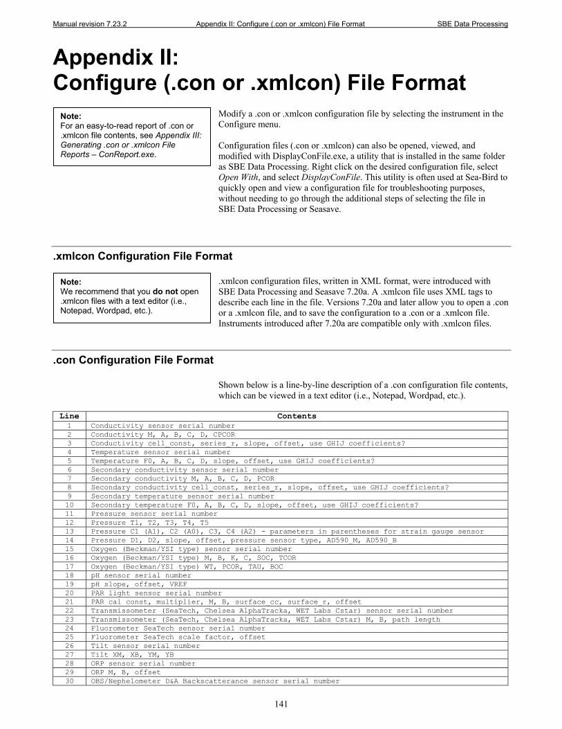
Manual revision 7.23.2 Appendix II: Configure (.con or .xmlcon) File Format SBE Data Processing
141
Appendix II: Configure (.con or .xmlcon) File Format
Modify a .con or .xmlcon configuration file by selecting the instrument in the Configure menu. Configuration files (.con or .xmlcon) can also be opened, viewed, and modified with DisplayConFile.exe, a utility that is installed in the same folder as SBE Data Processing. Right click on the desired configuration file, select Open With, and select DisplayConFile. This utility is often used at Sea-Bird to quickly open and view a configuration file for troubleshooting purposes, without needing to go through the additional steps of selecting the file in SBE Data Processing or Seasave.
.xmlcon Configuration File Format .xmlcon configuration files, written in XML format, were introduced with SBE Data Processing and Seasave 7.20a. A .xmlcon file uses XML tags to describe each line in the file. Versions 7.20a and later allow you to open a .con or a .xmlcon file, and to save the configuration to a .con or a .xmlcon file. Instruments introduced after 7.20a are compatible only with .xmlcon files.
.con Configuration File Format Shown below is a line-by-line description of a .con configuration file contents, which can be viewed in a text editor (i.e., Notepad, Wordpad, etc.).
Line Contents 1 Conductivity sensor serial number 2 Conductivity M, A, B, C, D, CPCOR 3 Conductivity cell_const, series_r, slope, offset, use GHIJ coefficients? 4 Temperature sensor serial number 5 Temperature F0, A, B, C, D, slope, offset, use GHIJ coefficients? 6 Secondary conductivity sensor serial number 7 Secondary conductivity M, A, B, C, D, PCOR 8 Secondary conductivity cell_const, series_r, slope, offset, use GHIJ coefficients? 9 Secondary temperature sensor serial number 10 Secondary temperature F0, A, B, C, D, slope, offset, use GHIJ coefficients? 11 Pressure sensor serial number 12 Pressure T1, T2, T3, T4, T5 13 Pressure C1 (A1), C2 (A0), C3, C4 (A2) - parameters in parentheses for strain gauge sensor 14 Pressure D1, D2, slope, offset, pressure sensor type, AD590_M, AD590_B 15 Oxygen (Beckman/YSI type) sensor serial number 16 Oxygen (Beckman/YSI type) M, B, K, C, SOC, TCOR 17 Oxygen (Beckman/YSI type) WT, PCOR, TAU, BOC 18 pH sensor serial number 19 pH slope, offset, VREF 20 PAR light sensor serial number 21 PAR cal const, multiplier, M, B, surface_cc, surface_r, offset 22 Transmissometer (SeaTech, Chelsea AlphaTracka, WET Labs Cstar) sensor serial number 23 Transmissometer (SeaTech, Chelsea AlphaTracka, WET Labs Cstar) M, B, path length 24 Fluorometer SeaTech sensor serial number 25 Fluorometer SeaTech scale factor, offset 26 Tilt sensor serial number 27 Tilt XM, XB, YM, YB 28 ORP sensor serial number 29 ORP M, B, offset 30 OBS/Nephelometer D&A Backscatterance sensor serial number
Note: For an easy-to-read report of .con or .xmlcon file contents, see Appendix III: Generating .con or .xmlcon File Reports – ConReport.exe.
Note: We recommend that you do not open .xmlcon files with a text editor (i.e., Notepad, Wordpad, etc.).
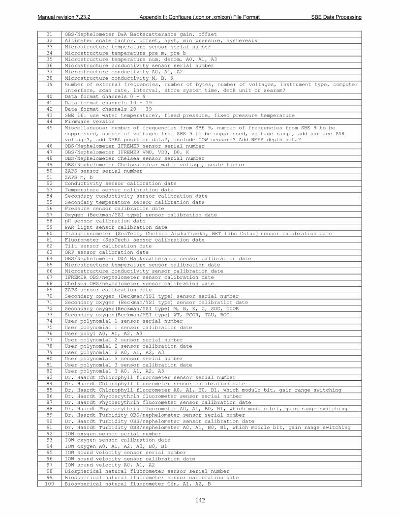
Manual revision 7.23.2 Appendix II: Configure (.con or .xmlcon) File Format SBE Data Processing
142
31 OBS/Nephelometer D&A Backscatterance gain, offset 32 Altimeter scale factor, offset, hyst, min pressure, hysteresis 33 Microstructure temperature sensor serial number 34 Microstructure temperature pre_m, pre_b 35 Microstructure temperature num, denom, A0, A1, A3 36 Microstructure conductivity sensor serial number 37 Microstructure conductivity A0, A1, A2 38 Microstructure conductivity M, B, R 39 Number of external frequencies, number of bytes, number of voltages, instrument type, computer
interface, scan rate, interval, store system time, deck unit or searam? 40 Data format channels 0 - 9 41 Data format channels 10 - 19 42 Data format channels 20 - 39 43 SBE 16: use water temperature?, fixed pressure, fixed pressure temperature 44 Firmware version 45 Miscellaneous: number of frequencies from SBE 9, number of frequencies from SBE 9 to be
suppressed, number of voltages from SBE 9 to be suppressed, voltage range, add surface PAR voltage?, add NMEA position data?, include IOW sensors? Add NMEA depth data?
46 OBS/Nephelometer IFREMER sensor serial number 47 OBS/Nephelometer IFREMER VM0, VD0, D0, K 48 OBS/Nephelometer Chelsea sensor serial number 49 OBS/Nephelometer Chelsea clear water voltage, scale factor 50 ZAPS sensor serial number 51 ZAPS m, b 52 Conductivity sensor calibration date 53 Temperature sensor calibration date 54 Secondary conductivity sensor calibration date 55 Secondary temperature sensor calibration date 56 Pressure sensor calibration date 57 Oxygen (Beckman/YSI type) sensor calibration date 58 pH sensor calibration date 59 PAR light sensor calibration date 60 Transmissometer (SeaTech, Chelsea AlphaTracka, WET Labs Cstar) sensor calibration date 61 Fluorometer (SeaTech) sensor calibration date 62 Tilt sensor calibration date 63 ORP sensor calibration date 64 OBS/Nephelometer D&A Backscatterance sensor calibration date 65 Microstructure temperature sensor calibration date 66 Microstructure conductivity sensor calibration date 67 IFREMER OBS/nephelometer sensor calibration date 68 Chelsea OBS/nephelometer sensor calibration date 69 ZAPS sensor calibration date 70 Secondary oxygen (Beckman/YSI type) sensor serial number 71 Secondary oxygen (Beckman/YSI type) sensor calibration date 72 Secondary oxygen(Beckman/YSI type) M, B, K, C, SOC, TCOR 73 Secondary oxygen(Beckman/YSI type) WT, PCOR, TAU, BOC 74 User polynomial 1 sensor serial number 75 User polynomial 1 sensor calibration date 76 User poly1 A0, A1, A2, A3 77 User polynomial 2 sensor serial number 78 User polynomial 2 sensor calibration date 79 User polynomial 2 A0, A1, A2, A3 80 User polynomial 3 sensor serial number 81 User polynomial 3 sensor calibration date 82 User polynomial 3 A0, A1, A2, A3 83 Dr. Haardt Chlorophyll fluorometer sensor serial number 84 Dr. Haardt Chlorophyll fluorometer sensor calibration date 85 Dr. Haardt Chlorophyll fluorometer A0, A1, B0, B1, which modulo bit, gain range switching 86 Dr. Haardt Phycoerythrin fluorometer sensor serial number 87 Dr. Haardt Phycoerythrin fluorometer sensor calibration date 88 Dr. Haardt Phycoerythrin fluorometer A0, A1, B0, B1, which modulo bit, gain range switching 89 Dr. Haardt Turbidity OBS/nephelometer sensor serial number 90 Dr. Haardt Turbidity OBS/nephelometer sensor calibration date 91 Dr. Haardt Turbidity OBS/nephelometer A0, A1, B0, B1, which modulo bit, gain range switching 92 IOW oxygen sensor serial number 93 IOW oxygen sensor calibration date 94 IOW oxygen A0, A1, A2, A3, B0, B1 95 IOW sound velocity sensor serial number 96 IOW sound velocity sensor calibration date 97 IOW sound velocity A0, A1, A2 98 Biospherical natural fluorometer sensor serial number 99 Biospherical natural fluorometer sensor calibration date 100 Biospherical natural fluorometer Cfn, A1, A2, B
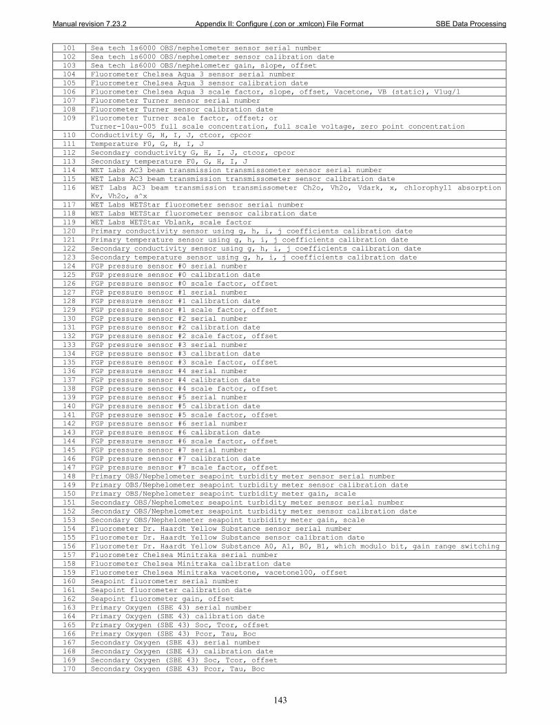
Manual revision 7.23.2 Appendix II: Configure (.con or .xmlcon) File Format SBE Data Processing
143
101 Sea tech ls6000 OBS/nephelometer sensor serial number 102 Sea tech ls6000 OBS/nephelometer sensor calibration date 103 Sea tech ls6000 OBS/nephelometer gain, slope, offset 104 Fluorometer Chelsea Aqua 3 sensor serial number 105 Fluorometer Chelsea Aqua 3 sensor calibration date 106 Fluorometer Chelsea Aqua 3 scale factor, slope, offset, Vacetone, VB (static), V1ug/l 107 Fluorometer Turner sensor serial number 108 Fluorometer Turner sensor calibration date 109 Fluorometer Turner scale factor, offset; or
Turner-10au-005 full scale concentration, full scale voltage, zero point concentration 110 Conductivity G, H, I, J, ctcor, cpcor 111 Temperature F0, G, H, I, J 112 Secondary conductivity G, H, I, J, ctcor, cpcor 113 Secondary temperature F0, G, H, I, J 114 WET Labs AC3 beam transmission transmissometer sensor serial number 115 WET Labs AC3 beam transmission transmissometer sensor calibration date 116 WET Labs AC3 beam transmission transmissometer Ch2o, Vh2o, Vdark, x, chlorophyll absorption
Kv, Vh2o, a^x 117 WET Labs WETStar fluorometer sensor serial number 118 WET Labs WETStar fluorometer sensor calibration date 119 WET Labs WETStar Vblank, scale factor 120 Primary conductivity sensor using g, h, i, j coefficients calibration date 121 Primary temperature sensor using g, h, i, j coefficients calibration date 122 Secondary conductivity sensor using g, h, i, j coefficients calibration date 123 Secondary temperature sensor using g, h, i, j coefficients calibration date 124 FGP pressure sensor #0 serial number 125 FGP pressure sensor #0 calibration date 126 FGP pressure sensor #0 scale factor, offset 127 FGP pressure sensor #1 serial number 128 FGP pressure sensor #1 calibration date 129 FGP pressure sensor #1 scale factor, offset 130 FGP pressure sensor #2 serial number 131 FGP pressure sensor #2 calibration date 132 FGP pressure sensor #2 scale factor, offset 133 FGP pressure sensor #3 serial number 134 FGP pressure sensor #3 calibration date 135 FGP pressure sensor #3 scale factor, offset 136 FGP pressure sensor #4 serial number 137 FGP pressure sensor #4 calibration date 138 FGP pressure sensor #4 scale factor, offset 139 FGP pressure sensor #5 serial number 140 FGP pressure sensor #5 calibration date 141 FGP pressure sensor #5 scale factor, offset 142 FGP pressure sensor #6 serial number 143 FGP pressure sensor #6 calibration date 144 FGP pressure sensor #6 scale factor, offset 145 FGP pressure sensor #7 serial number 146 FGP pressure sensor #7 calibration date 147 FGP pressure sensor #7 scale factor, offset 148 Primary OBS/Nephelometer seapoint turbidity meter sensor serial number 149 Primary OBS/Nephelometer seapoint turbidity meter sensor calibration date 150 Primary OBS/Nephelometer seapoint turbidity meter gain, scale 151 Secondary OBS/Nephelometer seapoint turbidity meter sensor serial number 152 Secondary OBS/Nephelometer seapoint turbidity meter sensor calibration date 153 Secondary OBS/Nephelometer seapoint turbidity meter gain, scale 154 Fluorometer Dr. Haardt Yellow Substance sensor serial number 155 Fluorometer Dr. Haardt Yellow Substance sensor calibration date 156 Fluorometer Dr. Haardt Yellow Substance A0, A1, B0, B1, which modulo bit, gain range switching 157 Fluorometer Chelsea Minitraka serial number 158 Fluorometer Chelsea Minitraka calibration date 159 Fluorometer Chelsea Minitraka vacetone, vacetone100, offset 160 Seapoint fluorometer serial number 161 Seapoint fluorometer calibration date 162 Seapoint fluorometer gain, offset 163 Primary Oxygen (SBE 43) serial number 164 Primary Oxygen (SBE 43) calibration date 165 Primary Oxygen (SBE 43) Soc, Tcor, offset 166 Primary Oxygen (SBE 43) Pcor, Tau, Boc 167 Secondary Oxygen (SBE 43) serial number 168 Secondary Oxygen (SBE 43) calibration date 169 Secondary Oxygen (SBE 43) Soc, Tcor, offset 170 Secondary Oxygen (SBE 43) Pcor, Tau, Boc
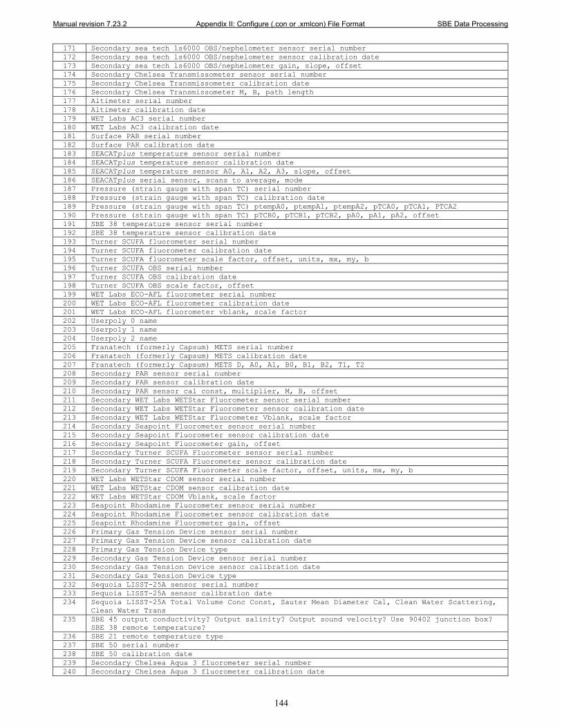
Manual revision 7.23.2 Appendix II: Configure (.con or .xmlcon) File Format SBE Data Processing
144
171 Secondary sea tech ls6000 OBS/nephelometer sensor serial number 172 Secondary sea tech ls6000 OBS/nephelometer sensor calibration date 173 Secondary sea tech ls6000 OBS/nephelometer gain, slope, offset 174 Secondary Chelsea Transmissometer sensor serial number 175 Secondary Chelsea Transmissometer calibration date 176 Secondary Chelsea Transmissometer M, B, path length 177 Altimeter serial number 178 Altimeter calibration date 179 WET Labs AC3 serial number 180 WET Labs AC3 calibration date 181 Surface PAR serial number 182 Surface PAR calibration date 183 SEACATplus temperature sensor serial number 184 SEACATplus temperature sensor calibration date 185 SEACATplus temperature sensor A0, A1, A2, A3, slope, offset 186 SEACATplus serial sensor, scans to average, mode 187 Pressure (strain gauge with span TC) serial number 188 Pressure (strain gauge with span TC) calibration date 189 Pressure (strain gauge with span TC) ptempA0, ptempA1, ptempA2, pTCA0, pTCA1, PTCA2 190 Pressure (strain gauge with span TC) pTCB0, pTCB1, pTCB2, pA0, pA1, pA2, offset 191 SBE 38 temperature sensor serial number 192 SBE 38 temperature sensor calibration date 193 Turner SCUFA fluorometer serial number 194 Turner SCUFA fluorometer calibration date 195 Turner SCUFA fluorometer scale factor, offset, units, mx, my, b 196 Turner SCUFA OBS serial number 197 Turner SCUFA OBS calibration date 198 Turner SCUFA OBS scale factor, offset 199 WET Labs ECO-AFL fluorometer serial number 200 WET Labs ECO-AFL fluorometer calibration date 201 WET Labs ECO-AFL fluorometer vblank, scale factor 202 Userpoly 0 name 203 Userpoly 1 name 204 Userpoly 2 name 205 Franatech (formerly Capsum) METS serial number 206 Franatech (formerly Capsum) METS calibration date 207 Franatech (formerly Capsum) METS D, A0, A1, B0, B1, B2, T1, T2 208 Secondary PAR sensor serial number 209 Secondary PAR sensor calibration date 210 Secondary PAR sensor cal const, multiplier, M, B, offset 211 Secondary WET Labs WETStar Fluorometer sensor serial number 212 Secondary WET Labs WETStar Fluorometer sensor calibration date 213 Secondary WET Labs WETStar Fluorometer Vblank, scale factor 214 Secondary Seapoint Fluorometer sensor serial number 215 Secondary Seapoint Fluorometer sensor calibration date 216 Secondary Seapoint Fluorometer gain, offset 217 Secondary Turner SCUFA Fluorometer sensor serial number 218 Secondary Turner SCUFA Fluorometer sensor calibration date 219 Secondary Turner SCUFA Fluorometer scale factor, offset, units, mx, my, b 220 WET Labs WETStar CDOM sensor serial number 221 WET Labs WETStar CDOM sensor calibration date 222 WET Labs WETStar CDOM Vblank, scale factor 223 Seapoint Rhodamine Fluorometer sensor serial number 224 Seapoint Rhodamine Fluorometer sensor calibration date 225 Seapoint Rhodamine Fluorometer gain, offset 226 Primary Gas Tension Device sensor serial number 227 Primary Gas Tension Device sensor calibration date 228 Primary Gas Tension Device type 229 Secondary Gas Tension Device sensor serial number 230 Secondary Gas Tension Device sensor calibration date 231 Secondary Gas Tension Device type 232 Sequoia LISST-25A sensor serial number 233 Sequoia LISST-25A sensor calibration date 234 Sequoia LISST-25A Total Volume Conc Const, Sauter Mean Diameter Cal, Clean Water Scattering,
Clean Water Trans 235 SBE 45 output conductivity? Output salinity? Output sound velocity? Use 90402 junction box?
SBE 38 remote temperature? 236 SBE 21 remote temperature type 237 SBE 50 serial number 238 SBE 50 calibration date 239 Secondary Chelsea Aqua 3 fluorometer serial number 240 Secondary Chelsea Aqua 3 fluorometer calibration date
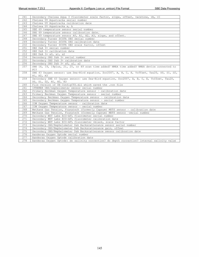
Manual revision 7.23.2 Appendix II: Configure (.con or .xmlcon) File Format SBE Data Processing
145
241 Secondary Chelsea Aqua 3 fluorometer scale factor, slope, offset, vacetone, vb, v1 242 Chelsea UV Aquatracka serial number 243 Chelsea UV Aquatracka calibration date 244 Chelsea UV Aquatracka a, b 245 SBE 49 temperature sensor serial number 246 SBE 49 temperature sensor calibration date. 247 SBE 49 temperature sensor A0, A1, A2, A3, slope, and offset. 248 Secondary Turner SCUFA OBS serial number 249 Secondary Turner SCUFA OBS calibration date 250 Secondary Turner SCUFA OBS scale factor, offset 251 OBS D&A 3+ serial number 252 OBS D&A 3+ calibration date 253 OBS D&A 3+ a0, a1, a2 254 Secondary OBS D&A 3+ serial number 255 Secondary OBS D&A 3+ calibration date 256 Secondary OBS D&A 3+ a0, a1, a2 257 SBE 16, 19, 19plus, 21, 25, or 49 scan time added? NMEA time added? NMEA device connected to
PC? 258 SBE 43 Oxygen sensor: use Sea-Bird equation, Soc2007, A, B, C, E, Voffset, Tau20, D0, D1, D2,
H1, H2, H3 259 Secondary SBE 43 Oxygen sensor: use Sea-Bird equation, Soc2007, A, B, C, E, Voffset, Tau20,
D0, D1, D2, H1, H2, H3 260 File version of SB_ConfigCTD.dll which saved the .con file 261 IFREMER OBS/nephelometer sensor serial number 262 Primary Beckman Oxygen Temperature sensor – calibration date 263 Primary Beckman Oxygen Temperature sensor – serial number 264 Secondary Beckman Oxygen Temperature sensor – calibration date 265 Secondary Beckman Oxygen Temperature sensor – serial number 266 IOW Oxygen Temperature sensor – calibration date 267 IOW Oxygen Temperature sensor – serial number 268 Methane Gas Tension, Franatech (formerly Capsum) METS sensor – calibration date 269 Methane Gas Tension, Franatech (formerly Capsum) METS sensor –serial number 270 Secondary WET Labs ECO-AFL fluorometer serial number 271 Secondary WET Labs ECO-AFL fluorometer calibration date 272 Secondary WET Labs ECO-AFL fluorometer vblank, scale factor 273 Secondary OBS/Nephelometer D&A Backscatterance sensor serial number 274 Secondary OBS/Nephelometer D&A Backscatterance gain, offset 275 Secondary OBS/Nephelometer D&A Backscatterance sensor calibration date 276 Aanderaa Oxygen Optode serial number 277 Aanderaa Oxygen Optode calibration date 278 Aanderaa Oxygen Optode: do salinity correction? do depth correction? internal salinity value
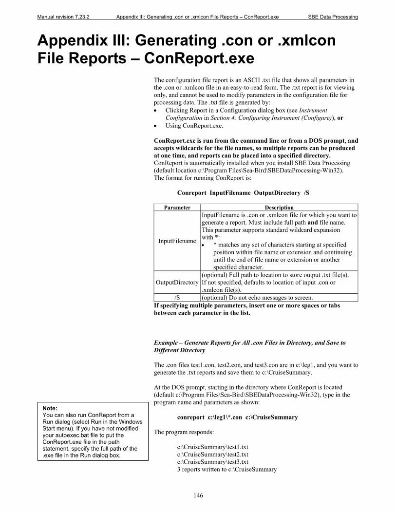
Manual revision 7.23.2 Appendix III: Generating .con or .xmlcon File Reports – ConReport.exe SBE Data Processing
146
Appendix III: Generating .con or .xmlcon File Reports – ConReport.exe
The configuration file report is an ASCII .txt file that shows all parameters in the .con or .xmlcon file in an easy-to-read form. The .txt report is for viewing only, and cannot be used to modify parameters in the configuration file for processing data. The .txt file is generated by: • Clicking Report in a Configuration dialog box (see Instrument
Configuration in Section 4: Configuring Instrument (Configure)), or • Using ConReport.exe. ConReport.exe is run from the command line or from a DOS prompt, and accepts wildcards for the file names, so multiple reports can be produced at one time, and reports can be placed into a specified directory. ConReport is automatically installed when you install SBE Data Processing (default location c:\Program Files\Sea-Bird\SBEDataProcessing-Win32). The format for running ConReport is:
Conreport InputFilename OutputDirectory /S
Parameter Description
InputFilename
InputFilename is .con or .xmlcon file for which you want to generate a report. Must include full path and file name. This parameter supports standard wildcard expansion with *: • * matches any set of characters starting at specified
position within file name or extension and continuing until the end of file name or extension or another specified character.
OutputDirectory (optional) Full path to location to store output .txt file(s). If not specified, defaults to location of input .con or .xmlcon file(s).
/S (optional) Do not echo messages to screen. If specifying multiple parameters, insert one or more spaces or tabs between each parameter in the list. Example – Generate Reports for All .con Files in Directory, and Save to Different Directory The .con files test1.con, test2.con, and test3.con are in c:\leg1, and you want to generate the .txt reports and save them to c:\CruiseSummary. At the DOS prompt, starting in the directory where ConReport is located (default c:\Program Files\Sea-Bird\SBEDataProcessing-Win32), type in the program name and parameters as shown:
conreport c:\leg1\*.con c:\CruiseSummary The program responds:
c:\CruiseSummary\test1.txt c:\CruiseSummary\test2.txt c:\CruiseSummary\test3.txt 3 reports written to c:\CruiseSummary
Note: You can also run ConReport from a Run dialog (select Run in the Windows Start menu). If you have not modified your autoexec.bat file to put the ConReport.exe file in the path statement, specify the full path of the .exe file in the Run dialog box.
Manual revision 7.23.2 Appendix IV: Software Problems SBE Data Processing
147
Appendix IV: Software Problems
Considerable effort has been made to test and check this software before its release. However, because of the wide range of instruments that Sea-Bird produces (and interfaces with) and the many applications that these instruments are used in, there may be software problems that have not been discovered and corrected. If a problem occurs, please contact us via phone (425-643-9866), email ([email protected]), or fax (425-643-9954) with the following information: • Instrument serial number • Version of the software originally shipped with the instrument • Version of the software you are attempting to run • Complete description of the problem you are having If the problem involves the configuration or setup of the software, in most cases a phone call to Sea-Bird will be sufficient to solve the problem. If you phone, we would appreciate it if you would be ready to run the software during the phone conversation. If the problem involves data processing, you may be asked to send a sample of the data to Sea-Bird for evaluation.
Manual revision 7.23.2 Appendix V: Derived Parameter Formulas (EOS-80; Practical Salinity) SBE Data Processing
148
Appendix V: Derived Parameter Formulas (EOS-80; Practical Salinity)
For formulas for the calculation of conductivity, temperature, and pressure, see the calibration sheets for your instrument. Formulas for the computation of salinity, density, potential temperature, specific volume anomaly, and sound velocity were obtained from "Algorithms for computation of fundamental properties of seawater", by N.P. Fofonoff and R.C Millard Jr.; Unesco technical papers in marine science #44, 1983. • Temperature used for calculating derived variables is IPTS-68, except as
noted. Following the recommendation of JPOTS, T68 is assumed to be 1.00024 * T90 (-2 to 35 °C).
• Salinity is PSS-78 (Practical Salinity) (see Application Note 14: 1978 Practical Salinity Scale). By definition, PSS-78 is valid only in the range of 2 to 42 psu. Sea-Bird uses the PSS-78 algorithm in our software, without regard to those limitations on the valid range. Unesco technical papers in marine science 62 "Salinity and density of seawater: Tables for high salinities (42 to 50)" provides a method for calculating salinity in the higher range (http://unesdoc.unesco.org/images/0009/000964/096451mb.pdf).
Equations / descriptions are provided for the following parameters:
• density (density, sigma-theta, sigma-1, sigma-2, sigma-4, sigma-t) • thermosteric anomaly • specific volume • specific volume anomaly • geopotential anomaly • dynamic meters • depth (salt water, fresh water) • seafloor depth (salt water, fresh water) • Practical Salinity (psu) • sound velocity (Chen-Millero, DelGrosso, Wilson) • average sound velocity • potential temperature (reference pressure = 0.0 decibars) • potential temperature anomaly • plume anomaly • specific conductivity • oxygen (if input file contains pressure, temperature, and either
conductivity or salinity, and has not been averaged into pressure or depth bins) - also requires oxygen signal (for SBE 43), oxygen current and oxygen temperature (for SBE 13 or 23), or oxygen phase and thermistor voltage (SBE 63)
• oxygen saturation • oxygen percent saturation • nitrogen saturation • derivative variables (descent rate and acceleration) - if input file has not
been averaged into pressure or depth bins • corrected irradiance (CPAR)
Notes: • Algorithms used for calculation of
derived parameters in Data Conversion, Derive, Sea Plot, SeaCalc III [EOS-80 (Practical Salinity) tab], and Seasave are identical, except as noted in this section, and are based on EOS-80 equations (Practical Salinity).
• Calculation of Absolute Salinity and associated parameters (TEOS-10) is available in Derive TEOS-10 and SeaCalc III [TEOS-10 (Absolute Salinity) tab]. Once they are calculated in Derive TEOS-10, they can be plotted in Sea Plot. See Section 6: Data Processing Modules and Section 9: Miscellaneous Module – SeaCalc III.
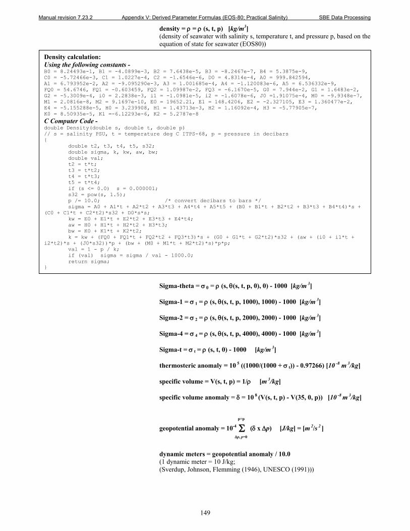
Manual revision 7.23.2 Appendix V: Derived Parameter Formulas (EOS-80; Practical Salinity) SBE Data Processing
149
density = ρ = ρ (s, t, p) [kg/m3] (density of seawater with salinity s, temperature t, and pressure p, based on the equation of state for seawater (EOS80))
Sigma-theta = σ θ = ρ (s, θ(s, t, p, 0), 0) - 1000 [kg/m 3] Sigma-1 = σ 1 = ρ (s, θ(s, t, p, 1000), 1000) - 1000 [kg/m 3] Sigma-2 = σ 2 = ρ (s, θ(s, t, p, 2000), 2000) - 1000 [kg/m 3] Sigma-4 = σ 4 = ρ (s, θ(s, t, p, 4000), 4000) - 1000 [kg/m 3] Sigma-t = σ t = ρ (s, t, 0) - 1000 [kg/m 3]
thermosteric anomaly = 10 5 ((1000/(1000 + σ t)) - 0.97266) [10 -8 m 3/kg] specific volume = V(s, t, p) = 1/ρ [m 3/kg] specific volume anomaly = δ = 10 8 (V(s, t, p) - V(35, 0, p)) [10 -8 m 3/kg] p=p
geopotential anomaly = 10-4 Σ (δ x ∆p) [J/kg] = [m 2/s 2 ]
∆p, p=0
dynamic meters = geopotential anomaly / 10.0 (1 dynamic meter = 10 J/kg; (Sverdup, Johnson, Flemming (1946), UNESCO (1991)))
Density calculation: Using the following constants - B0 = 8.24493e-1, B1 = -4.0899e-3, B2 = 7.6438e-5, B3 = -8.2467e-7, B4 = 5.3875e-9, C0 = -5.72466e-3, C1 = 1.0227e-4, C2 = -1.6546e-6, D0 = 4.8314e-4, A0 = 999.842594, A1 = 6.793952e-2, A2 = -9.095290e-3, A3 = 1.001685e-4, A4 = -1.120083e-6, A5 = 6.536332e-9, FQ0 = 54.6746, FQ1 = -0.603459, FQ2 = 1.09987e-2, FQ3 = -6.1670e-5, G0 = 7.944e-2, G1 = 1.6483e-2, G2 = -5.3009e-4, i0 = 2.2838e-3, i1 = -1.0981e-5, i2 = -1.6078e-6, J0 =1.91075e-4, M0 = -9.9348e-7, M1 = 2.0816e-8, M2 = 9.1697e-10, E0 = 19652.21, E1 = 148.4206, E2 = -2.327105, E3 = 1.360477e-2, E4 = -5.155288e-5, H0 = 3.239908, H1 = 1.43713e-3, H2 = 1.16092e-4, H3 = -5.77905e-7, K0 = 8.50935e-5, K1 =-6.12293e-6, K2 = 5.2787e-8
C Computer Code - double Density(double s, double t, double p) // s = salinity PSU, t = temperature deg C ITPS-68, p = pressure in decibars { double t2, t3, t4, t5, s32; double sigma, k, kw, aw, bw; double val; t2 = t*t; t3 = t*t2; t4 = t*t3; t5 = t*t4; if (s <= 0.0) s = 0.000001; s32 = pow(s, 1.5); p /= 10.0; /* convert decibars to bars */ sigma = A0 + A1*t + A2*t2 + A3*t3 + A4*t4 + A5*t5 + (B0 + B1*t + B2*t2 + B3*t3 + B4*t4)*s + (C0 + C1*t + C2*t2)*s32 + D0*s*s; kw = E0 + E1*t + E2*t2 + E3*t3 + E4*t4; aw = H0 + H1*t + H2*t2 + H3*t3; bw = K0 + K1*t + K2*t2; k = kw + (FQ0 + FQ1*t + FQ2*t2 + FQ3*t3)*s + (G0 + G1*t + G2*t2)*s32 + (aw + (i0 + i1*t + i2*t2)*s + (J0*s32))*p + (bw + (M0 + M1*t + M2*t2)*s)*p*p; val = 1 - p / k; if (val) sigma = sigma / val - 1000.0; return sigma; }

Manual revision 7.23.2 Appendix V: Derived Parameter Formulas (EOS-80; Practical Salinity) SBE Data Processing
150
depth = [m] (When you select salt water depth as a derived variable, SBE Data Processing prompts you to input the latitude, which is needed to calculate local gravity. It uses the user-input value, unless latitude is written in the input data file header [from a NMEA navigation device]. If latitude is in the input file header, SBE Data Processing uses the header value, and ignores the user-input latitude.).
seafloor depth = depth + altimeter reading [m]
Depth calculation: C Computer Code – // Depth double Depth(int dtype, double p, double latitude) // dtype = fresh water or salt water, p = pressure in decibars, latitude in degrees { double x, d, gr; if (dtype == FRESH_WATER) /* fresh water */ d = p * 1.019716; else { /* salt water */ x = sin(latitude / 57.29578); x = x * x; gr = 9.780318 * (1.0 + (5.2788e-3 + 2.36e-5 * x) * x) + 1.092e-6 * p; d = (((-1.82e-15 * p + 2.279e-10) * p - 2.2512e-5) * p + 9.72659) * p; if (gr) d /= gr; } return(d); }
Note: You can also enter the latitude on the Miscellaneous tab in Data Conversion or Derive, as applicable.
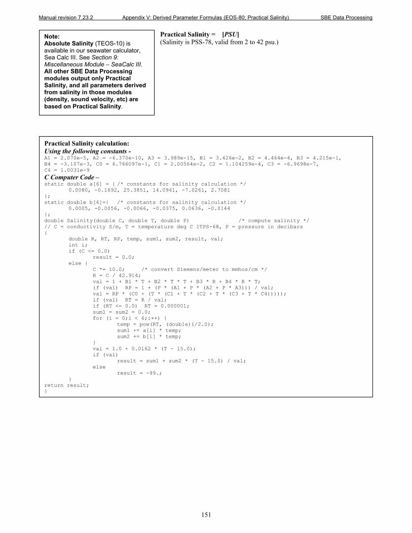
Manual revision 7.23.2 Appendix V: Derived Parameter Formulas (EOS-80; Practical Salinity) SBE Data Processing
151
Practical Salinity = [PSU] (Salinity is PSS-78, valid from 2 to 42 psu.)
Practical Salinity calculation: Using the following constants - A1 = 2.070e-5, A2 = -6.370e-10, A3 = 3.989e-15, B1 = 3.426e-2, B2 = 4.464e-4, B3 = 4.215e-1, B4 = -3.107e-3, C0 = 6.766097e-1, C1 = 2.00564e-2, C2 = 1.104259e-4, C3 = -6.9698e-7, C4 = 1.0031e-9
C Computer Code – static double a[6] = { /* constants for salinity calculation */ 0.0080, -0.1692, 25.3851, 14.0941, -7.0261, 2.7081 }; static double b[6]={ /* constants for salinity calculation */ 0.0005, -0.0056, -0.0066, -0.0375, 0.0636, -0.0144 }; double Salinity(double C, double T, double P) /* compute salinity */ // C = conductivity S/m, T = temperature deg C ITPS-68, P = pressure in decibars { double R, RT, RP, temp, sum1, sum2, result, val; int i; if (C <= 0.0) result = 0.0; else { C *= 10.0; /* convert Siemens/meter to mmhos/cm */ R = C / 42.914; val = 1 + B1 * T + B2 * T * T + B3 * R + B4 * R * T; if (val) RP = 1 + (P * (A1 + P * (A2 + P * A3))) / val; val = RP * (C0 + (T * (C1 + T * (C2 + T * (C3 + T * C4))))); if (val) RT = R / val; if (RT <= 0.0) RT = 0.000001; sum1 = sum2 = 0.0; for (i = 0;i < 6;i++) { temp = pow(RT, (double)i/2.0); sum1 += a[i] * temp; sum2 += b[i] * temp; } val = 1.0 + 0.0162 * (T - 15.0); if (val) result = sum1 + sum2 * (T - 15.0) / val; else result = -99.; } return result; }
Note: Absolute Salinity (TEOS-10) is available in our seawater calculator, Sea Calc III. See Section 9: Miscellaneous Module – SeaCalc III. All other SBE Data Processing modules output only Practical Salinity, and all parameters derived from salinity in those modules (density, sound velocity, etc) are based on Practical Salinity.
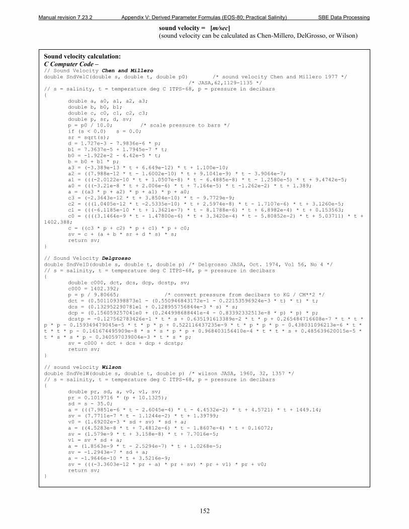
Manual revision 7.23.2 Appendix V: Derived Parameter Formulas (EOS-80; Practical Salinity) SBE Data Processing
152
sound velocity = [m/sec] (sound velocity can be calculated as Chen-Millero, DelGrosso, or Wilson)
Sound velocity calculation: C Computer Code – // Sound Velocity Chen and Millero double SndVelC(double s, double t, double p0) /* sound velocity Chen and Millero 1977 */ /* JASA,62,1129-1135 */ // s = salinity, t = temperature deg C ITPS-68, p = pressure in decibars { double a, a0, a1, a2, a3; double b, b0, b1; double c, c0, c1, c2, c3; double p, sr, d, sv; p = p0 / 10.0; /* scale pressure to bars */ if (s < 0.0) s = 0.0; sr = sqrt(s); d = 1.727e-3 - 7.9836e-6 * p; b1 = 7.3637e-5 + 1.7945e-7 * t; b0 = -1.922e-2 - 4.42e-5 * t; b = b0 + b1 * p; a3 = (-3.389e-13 * t + 6.649e-12) * t + 1.100e-10; a2 = ((7.988e-12 * t - 1.6002e-10) * t + 9.1041e-9) * t - 3.9064e-7; a1 = (((-2.0122e-10 * t + 1.0507e-8) * t - 6.4885e-8) * t - 1.2580e-5) * t + 9.4742e-5; a0 = (((-3.21e-8 * t + 2.006e-6) * t + 7.164e-5) * t -1.262e-2) * t + 1.389; a = ((a3 * p + a2) * p + a1) * p + a0; c3 = (-2.3643e-12 * t + 3.8504e-10) * t - 9.7729e-9; c2 = (((1.0405e-12 * t -2.5335e-10) * t + 2.5974e-8) * t - 1.7107e-6) * t + 3.1260e-5; c1 = (((-6.1185e-10 * t + 1.3621e-7) * t - 8.1788e-6) * t + 6.8982e-4) * t + 0.153563; c0 = ((((3.1464e-9 * t - 1.47800e-6) * t + 3.3420e-4) * t - 5.80852e-2) * t + 5.03711) * t + 1402.388; c = ((c3 * p + c2) * p + c1) * p + c0; sv = c + (a + b * sr + d * s) * s; return sv; } // Sound Velocity Delgrosso double SndVelD(double s, double t, double p) /* Delgrosso JASA, Oct. 1974, Vol 56, No 4 */ // s = salinity, t = temperature deg C ITPS-68, p = pressure in decibars { double c000, dct, dcs, dcp, dcstp, sv; c000 = 1402.392; p = p / 9.80665; /* convert pressure from decibars to KG / CM**2 */ dct = (0.501109398873e1 - (0.550946843172e-1 - 0.22153596924e-3 * t) * t) * t; dcs = (0.132952290781e1 + 0.128955756844e-3 * s) * s; dcp = (0.156059257041e0 + (0.244998688441e-4 - 0.83392332513e-8 * p) * p) * p; dcstp = -0.127562783426e-1 * t * s + 0.635191613389e-2 * t * p + 0.265484716608e-7 * t * t * p * p - 0.159349479045e-5 * t * p * p + 0.522116437235e-9 * t * p * p * p - 0.438031096213e-6 * t * t * t * p - 0.161674495909e-8 * s * s * p * p + 0.968403156410e-4 * t * t * s + 0.485639620015e-5 * t * s * s * p - 0.340597039004e-3 * t * s * p; sv = c000 + dct + dcs + dcp + dcstp; return sv; } // sound velocity Wilson double SndVelW(double s, double t, double p) /* wilson JASA, 1960, 32, 1357 */ // s = salinity, t = temperature deg C ITPS-68, p = pressure in decibars { double pr, sd, a, v0, v1, sv; pr = 0.1019716 * (p + 10.1325); sd = s - 35.0; a = (((7.9851e-6 * t - 2.6045e-4) * t - 4.4532e-2) * t + 4.5721) * t + 1449.14; sv = (7.7711e-7 * t - 1.1244e-2) * t + 1.39799; v0 = (1.69202e-3 * sd + sv) * sd + a; a = ((4.5283e-8 * t + 7.4812e-6) * t - 1.8607e-4) * t + 0.16072; sv = (1.579e-9 * t + 3.158e-8) * t + 7.7016e-5; v1 = sv * sd + a; a = (1.8563e-9 * t - 2.5294e-7) * t + 1.0268e-5; sv = -1.2943e-7 * sd + a; a = -1.9646e-10 * t + 3.5216e-9; sv = (((-3.3603e-12 * pr + a) * pr + sv) * pr + v1) * pr + v0; return sv; }
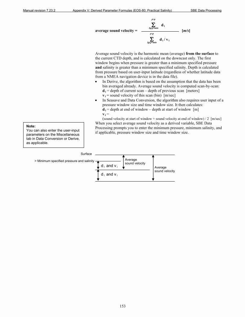
Manual revision 7.23.2 Appendix V: Derived Parameter Formulas (EOS-80; Practical Salinity) SBE Data Processing
153
average sound velocity = [m/s] Average sound velocity is the harmonic mean (average) from the surface to the current CTD depth, and is calculated on the downcast only. The first window begins when pressure is greater than a minimum specified pressure and salinity is greater than a minimum specified salinity. Depth is calculated from pressure based on user-input latitude (regardless of whether latitude data from a NMEA navigation device is in the data file). • In Derive, the algorithm is based on the assumption that the data has been
bin averaged already. Average sound velocity is computed scan-by-scan: d i = depth of current scan – depth of previous scan [meters] v i = sound velocity of this scan (bin) [m/sec]
• In Seasave and Data Conversion, the algorithm also requires user input of a pressure window size and time window size. It then calculates: d i = depth at end of window – depth at start of window [m] v i = (sound velocity at start of window + sound velocity at end of window) / 2 [m/sec]
When you select average sound velocity as a derived variable, SBE Data Processing prompts you to enter the minimum pressure, minimum salinity, and if applicable, pressure window size and time window size.
Surface
> Minimum specified pressure and salinity d i and v i
Average sound velocity
Average sound velocity
d i and v i
Σ d i ∆p,p=min
p=p
Σ d i / v i ∆p,p=min
p=p
Note: You can also enter the user-input parameters on the Miscellaneous tab in Data Conversion or Derive, as applicable.
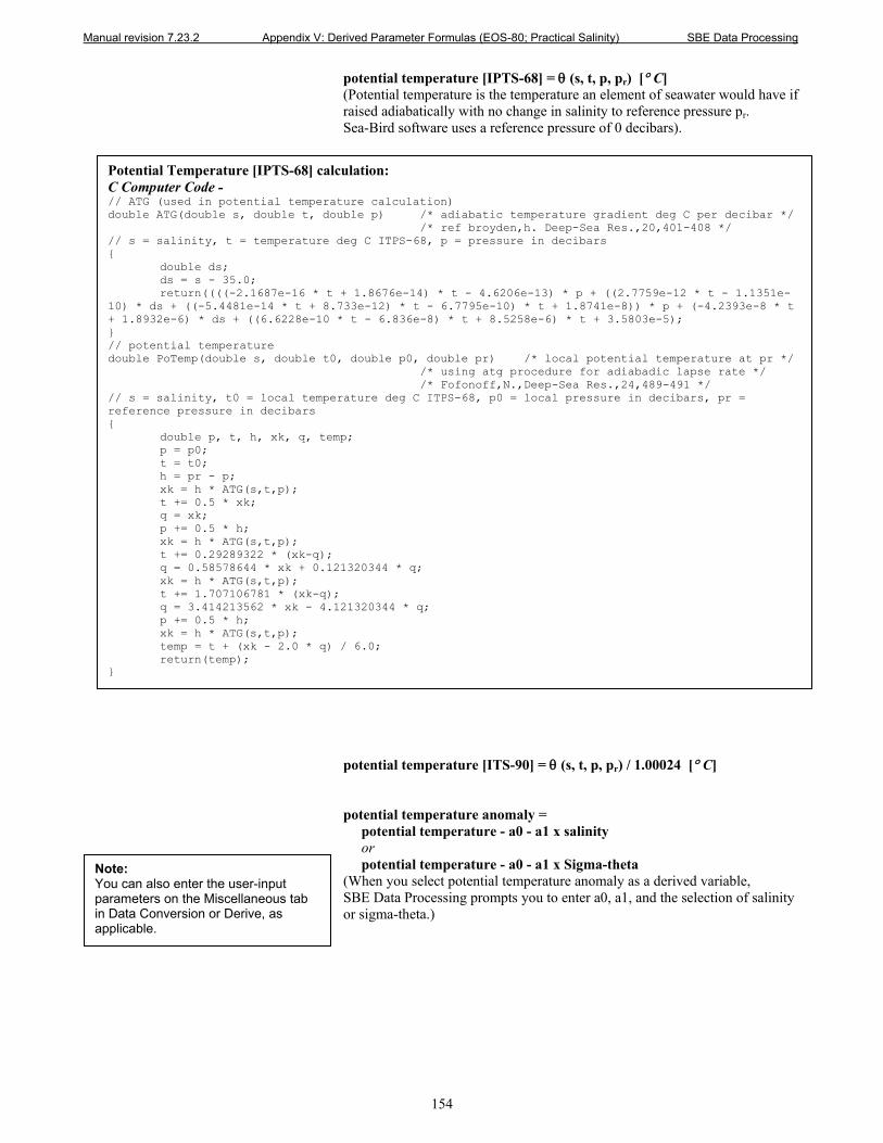
Manual revision 7.23.2 Appendix V: Derived Parameter Formulas (EOS-80; Practical Salinity) SBE Data Processing
154
potential temperature [IPTS-68] = θ (s, t, p, pr) [° C] (Potential temperature is the temperature an element of seawater would have if raised adiabatically with no change in salinity to reference pressure pr. Sea-Bird software uses a reference pressure of 0 decibars).
potential temperature [ITS-90] = θ (s, t, p, pr) / 1.00024 [° C] potential temperature anomaly = potential temperature - a0 - a1 x salinity or potential temperature - a0 - a1 x Sigma-theta (When you select potential temperature anomaly as a derived variable, SBE Data Processing prompts you to enter a0, a1, and the selection of salinity or sigma-theta.)
Potential Temperature [IPTS-68] calculation: C Computer Code - // ATG (used in potential temperature calculation) double ATG(double s, double t, double p) /* adiabatic temperature gradient deg C per decibar */ /* ref broyden,h. Deep-Sea Res.,20,401-408 */ // s = salinity, t = temperature deg C ITPS-68, p = pressure in decibars { double ds; ds = s - 35.0; return((((-2.1687e-16 * t + 1.8676e-14) * t - 4.6206e-13) * p + ((2.7759e-12 * t - 1.1351e-10) * ds + ((-5.4481e-14 * t + 8.733e-12) * t - 6.7795e-10) * t + 1.8741e-8)) * p + (-4.2393e-8 * t + 1.8932e-6) * ds + ((6.6228e-10 * t - 6.836e-8) * t + 8.5258e-6) * t + 3.5803e-5); } // potential temperature double PoTemp(double s, double t0, double p0, double pr) /* local potential temperature at pr */ /* using atg procedure for adiabadic lapse rate */ /* Fofonoff,N.,Deep-Sea Res.,24,489-491 */ // s = salinity, t0 = local temperature deg C ITPS-68, p0 = local pressure in decibars, pr = reference pressure in decibars { double p, t, h, xk, q, temp; p = p0; t = t0; h = pr - p; xk = h * ATG(s,t,p); t += 0.5 * xk; q = xk; p += 0.5 * h; xk = h * ATG(s,t,p); t += 0.29289322 * (xk-q); q = 0.58578644 * xk + 0.121320344 * q; xk = h * ATG(s,t,p); t += 1.707106781 * (xk-q); q = 3.414213562 * xk - 4.121320344 * q; p += 0.5 * h; xk = h * ATG(s,t,p); temp = t + (xk - 2.0 * q) / 6.0; return(temp); }
Note: You can also enter the user-input parameters on the Miscellaneous tab in Data Conversion or Derive, as applicable.
Manual revision 7.23.2 Appendix V: Derived Parameter Formulas (EOS-80; Practical Salinity) SBE Data Processing
155
plume anomaly = potential temperature (s, t, p, Reference Pressure) – Theta-B – Theta-Z / Salinity-Z * (salinity – Salinity-B) (When you select plume anomaly as a derived variable, SBE Data Processing prompts you to enter Theta-B, Salinity-B, Theta-Z / Salinity-Z, and Reference Pressure.) The plume anomaly equation is based on work in hydrothermal vent plumes. The algorithm used for identifying hydrothermal vent plumes uses potential temperature, gradient conditions in the region, vent salinity, and ambient seawater conditions adjacent to the vent. This function is specific to hydrothermal vent plumes, and more specifically, temperature and potential density anomalies. It is not a generic function for plume tracking (for example, not for wastewater plumes). One anomaly for one region and application does not necessarily apply to another type of anomaly in another region for a different application. The terms are specific to corrections for hydrothermal vent salinity and local hydrographic features near vents. They are likely not relevant to other applications in this exact form. If looking at wastewater plumes, you need to derive your own anomaly function that is specific to what it is you are looking for and that is defined to differentiate between surrounding waters and the wastewater plume waters. specific conductivity = (C * 10,000) / (1 + A * [T – 25]) [microS/cm] (C = conductivity (S/m), T = temperature (° C), A = thermal coefficient of conductivity for a natural salt solution [0.019 - 0.020]; Sea-Bird software uses 0.020.)
Notes: • You can also enter the user-input
parameters on the Miscellaneous tab in Data Conversion; plume anomaly is not available as a derived variable in Derive.
• Reference: Baker, E.T., Feely, R.A., Mottl, M.J., Sansone, F. T., Wheat, C.G., Resing, J.A., Lupton, J.E., "Hydrothermal plumes along the East Pacific Rise, 8° 40′ to 11° 50′ N: Plume distribution and relationship to the apparent magmatic budget", Earth and Planetary Science Letters 128 (1994) 1-17.
Manual revision 7.23.2 Appendix V: Derived Parameter Formulas (EOS-80; Practical Salinity) SBE Data Processing
156
Oxygen [ml/l] is calculated as described in Application Note 64: SBE 43 Dissolved Oxygen Sensor or Application Note 13-1: SBE 13, 23, 30 Dissolved Oxygen Sensor Calibration & Deployment. When you select oxygen as a derived variable, Data Conversion prompts you to enter the window size (seconds), and asks if you want to apply the Tau correction and the hysteresis correction: • Tau correction – The Tau correction ([tau(T,P)*δV/δt] in SBE 43 or
[tau*doc/dt] in SBE 13 or 23) improves response of the measured signal in regions of large oxygen gradients. However, this term also amplifies residual noise in the signal (especially in deep water); in some situations this negative consequence overshadows gains in signal responsiveness. If the Tau correction is enabled, oxygen computed by Seasave and Data Conversion is somewhat different from values computed by Derive. Both algorithms compute the derivative of the oxygen signal with respect to time (with a user-input window size for calculating the derivative), using a linear regression to determine the slope. Seasave and Data Conversion compute the derivative looking backward in time, since they share common code and Seasave cannot use future values of oxygen while acquiring data in real time. Derive uses a centered window (equal number of points before and after the scan) to obtain a better estimate of the derivative. Use Seasave and Data Conversion to obtain a quick look at oxygen values; use Derive to obtain the most accurate values.
• Hysteresis correction (SBE 43 only, when using Sea-Bird equation) - Under extreme pressure, changes can occur in gas permeable Teflon membranes that affect their permeability characteristics. Some of these changes (plasticization and amorphous/crystalinity ratios) have long time constants and depend on the sensor’s time-pressure history. These slow processes result in hysteresis in long, deep casts. The hysteresis correction algorithm (using H1, H2, and H3 coefficients entered for the SBE 43 in the .con or .xmlcon file) operates through the entire data profile and corrects the oxygen voltage values for changes in membrane permeability as pressure varies. At each measurement, the correction to the membrane permeability is calculated based on the current pressure and how long the sensor spent at previous pressures. Hysteresis responses of membranes on individual SBE 43 sensors are very similar, and in most cases the default hysteresis parameters provide the accuracy specification of 2% of true value. For users requiring higher accuracy (±1 µmol/kg), the parameters can be fine-tuned, if a complete profile (descent and ascent) made preferably to greater than 3000 meters is available. H1, the effect’s amplitude, has a default of -0.033, but can range from -0.02 to -0.05 between sensors. H2, the effect’s non-linear component, has a default of 5000, and is a second-order parameter that does not require tuning between sensors. H3, the effect’s time constant, has a default of 1450 seconds, but can range from 1200 to 2000. Hysteresis can be eliminated by alternately adjusting H1 and H3 in the .con or .xmlcon file during analysis of the complete profile. Once established, these parameters should be stable, and can be used without adjustment on other casts with the same SBE 43.
When you select oxygen as a derived variable, Derive prompts you to enter the window size (seconds), and asks if you want to apply the Tau correction (described above for Data Conversion). You cannot apply the hysteresis correction in Derive, to prevent users from applying the correction to oxygen voltage in Data Conversion and then applying it again in Derive, providing erroneous results. oxygen [µmoles/kg] = oxygen [ml/l] Sigma-theta + 1000
44660
Note: You can also enter the oxygen window size, and enable / disable the Tau and hysteresis corrections, on the Miscellaneous tab in Data Conversion or Derive, as applicable.
Note: The hysteresis correction can be performed to calculate and output oxygen voltage and/or calculated oxygen (ml/l, etc.) in Data Conversion. Hysteresis-corrected voltage from Data Conversion can be further processed in other modules (such as Align CTD) before calculating oxygen values (ml/l, etc.) in Derive.
Note: Oxygen [ml/l] for the SBE 63 Optical Dissolved Oxygen Sensor is calculated as described in its manual. Tau and hysteresis corrections are not applicable to the SBE 63.
Manual revision 7.23.2 Appendix V: Derived Parameter Formulas (EOS-80; Practical Salinity) SBE Data Processing
157
Oxygen saturation is the theoretical saturation limit of the water at the local temperature and salinity value, but with local pressure reset to zero (1 atmosphere). This calculation represents what the local parcel of water could have absorbed from the atmosphere when it was last at the surface (p=0) but at the same (T,S) value. Oxygen saturation can be calculated as Garcia and Gordon, or Weiss –
Garcia and Gordon: Oxsol(T,S) = exp {A0 + A1(Ts) + A2(Ts) 2 + A3(Ts) 3 + A4(Ts) 4 + A5(Ts) 5 + S * [B0 + B1(Ts) + B2(Ts) 2 + B3(Ts) 3] + C0(S) 2} where • Oxsol(T,S) = oxygen saturation value (ml/l) • S = salinity (psu) • T = water temperature (ITS-90, oC) • Ts = ln [(298.15 – T) / (273.15 + T)] • A0 = 2.00907 A1 = 3.22014 A2 = 4.0501
A3 = 4.94457 A4 = - 0.256847 A5 = 3.88767 • B0 = -0.00624523 B1 = -0.00737614
B2 = -0.010341 B3 = -0.00817083 • C0 = -0.000000488682
Weiss: Oxsat(T,S) = exp {[A1 + A2 * (100/Ta) + A3 * ln(Ta/100) + A4 * ( Ta/100)] + S * [B1 + B2 * (Ta/100) + B3 * (Ta/100)2 ]} where • Oxsat(T,S) = oxygen saturation value (ml/l) • S = salinity (psu) • T = water temperature (IPTS-68, oC) • Ta = absolute water temperature (T + 273.15) • A1 = -173.4292 A2 = 249.6339 A3 = 143.3483 A4 = -21.8492 • B1 = -0.033096 B2 = 0.014259 B3 = -0.00170 Oxygen, percent saturation is the ratio of calculated oxygen to oxygen saturation, in percent: (Oxygen / Oxygen saturation) * 100%. The Oxygen Saturation value used in this calculation is the value that was used in the Oxygen calculation – • SBE 43 -if you selected the Sea-Bird equation in the .con or .xmlcon file,
the software uses the Garcia and Gordon Oxsol in this ratio; if you selected the Owens-Millard equation in the .con or .xmlcon file, the software uses the Weiss Oxsat in this ratio.
• SBE 13, 23, or 30 – the software uses the Weiss Oxsat for this ratio. Nitrogen saturation is the theoretical saturation limit of the water at the local temperature and salinity value, but with local pressure reset to zero (1 atmosphere). This calculation represents what the local parcel of water could have absorbed from the atmosphere when it was last at the surface (p=0) but at the same (T,S) value. N2sat(T,S) = exp {[A1 + A2 * (100/Ta) + A3 * ln(Ta/100) + A4 * (Ta/100) ] + S * [B1 + B2 * (Ta/100) + B3 * (Ta/100) 2 ]} where • N2Sat(T,S) = nitrogen saturation value (ml/l) • S = salinity (psu) • T = water temperature (oC) • Ta = absolute water temperature (oC + 273.15) • A1 = -172.4965 A2 = 248.4262 A3 = 143.0738 A4 = -21.7120 • B1 = -0.049781 B2 = 0.025018 B3 = -0.0034861
Notes: • The oxygen saturation equation
based on work from Garcia and Gordon (1992) reduces error in the Weiss (1970) parameterization at cold temperatures.
• As implemented in Sea-Bird software, the Garcia and Gordon equation is valid for -5 < T < 50 and 0 < S < 60. Outside of those ranges, the software returns a value of -99 for Oxsol.
• As implemented in Sea-Bird software, the Weiss equation is valid for -2 < T < 40 and 0 < S < 42. Outside of those ranges, the software returns a value of -99 for Oxsat.
Note: The nitrogen saturation equation is based on work from Weiss (1970).
Manual revision 7.23.2 Appendix V: Derived Parameter Formulas (EOS-80; Practical Salinity) SBE Data Processing
158
Descent rate and acceleration are computed by calculating the derivative of the pressure signal with respect to time (with a user-input window size for calculating the derivative), using a linear regression to determine the slope. Values computed by Seasave and Data Conversion are somewhat different from values computed by Derive. Seasave and Data Conversion compute the derivative looking backward in time (with a user-input window size), since they share common code and Seasave cannot use future values of pressure while acquiring data in real time. Derive uses a centered window (equal number of points before and after the scan; user-input window size) to obtain a better estimate of the derivative. Use Seasave and Data Conversion to obtain a quick look at descent rate and acceleration; use Derive to obtain the most accurate values. (When you select descent rate or acceleration as a derived variable, SBE Data Processing prompts you to enter the window size (seconds).)
Corrected Irradiance [CPAR] = 100 * ratio multiplier * underwater PAR / surface PAR [%] (Ratio multiplier = scaling factor used for comparing light fields of disparate intensity, input in .con or .xmlcon file entry for surface PAR sensor; Underwater PAR = underwater PAR data; Surface PAR = surface PAR data)
Note: You can also enter the descent rate and acceleration window size on the Miscellaneous tab in Data Conversion or Derive, as applicable.
Note: For complete description of ratio multiplier, see Application Note 11S (SBE 11plus Deck Unit) or 47 (SBE 33 or 36 Deck Unit).
Manual revision 7.23.2 Appendix VI: Output Variable Names SBE Data Processing
159
Appendix VI: Output Variable Names
This appendix provides a list of output variable names. The names vary, depending on whether you are viewing header information in a data file or viewing real-time data in Seasave. • Headers generated by modules in SBE Data Processing show
‘Short name: Full name’ in header. Example: # name 0 = prdM: Pressure, Strain Gauge [db] (# name 0 indicates that this is the header for the first data column; prdM is the Short name used in the software coding; Pressure, Strain Gauge [db] is the more descriptive Full name)
• Seasave’s scrolled display shows a ‘Friendly name’ in heading. Example: pr M (this is the Friendly name for Pressure, Strain Gauge [db]; pr indicates pressure and M indicates metric units)
• Seasave’s fixed display and plot display show 'Full name’. Example: Pressure, Strain Gauge [db] (this is the Full name)
For CTDs that support redundant sensors: Unless noted otherwise, derived variables are calculated only from primary sensor(s). Example: Sound Velocity [Chen-Millero, m/s] can be calculated from both primary and secondary temperature and conductivity sensors on an SBE 9plus (which supports secondary temperature and conductivity sensors), as indicated by the presence of both Sound Velocity [Chen-Millero, m/s] and Sound Velocity,2 [Chen-Millero, m/s] in the table. However, Average Sound Velocity [Chen-Millero, m/s] can only be calculated from the primary temperature and conductivity sensors (there is no entry for this variable with a 2). For some parameters, there are multiple entries in the table with the same meaning for the user (but different meanings for the software). Example: Short names of c_S/m, cond0S/m, and c0S/m all have long names of Conductivity [S/m]; these parameters all provide conductivity in S/m. However, the short names are different because of differences in the conductivity equation used by the software in the calculation (equation varies, depending on the CTD). All variable selections can be made in Seasave and in SBE Data Processing’s Derive module, except as noted. The list is in two parts: • Practical Salinity and related thermodynamic parameters (EOS-80), and
auxiliary sensor data • Absolute Salinity and related thermodynamic parameters (calculated in
and output by SBE Data Processing’s Derive TEOS-10 module)
Note: The Notes/Comments column in the table below indicates 1st sensor, 2nd sensor, etc. For parameters calculated from multiple sensors (for example, salinity is a function of temperature, conductivity, and pressure), 1st refers to the 1st sensor T-C pair, 2nd refers to the secondary T-C pair.
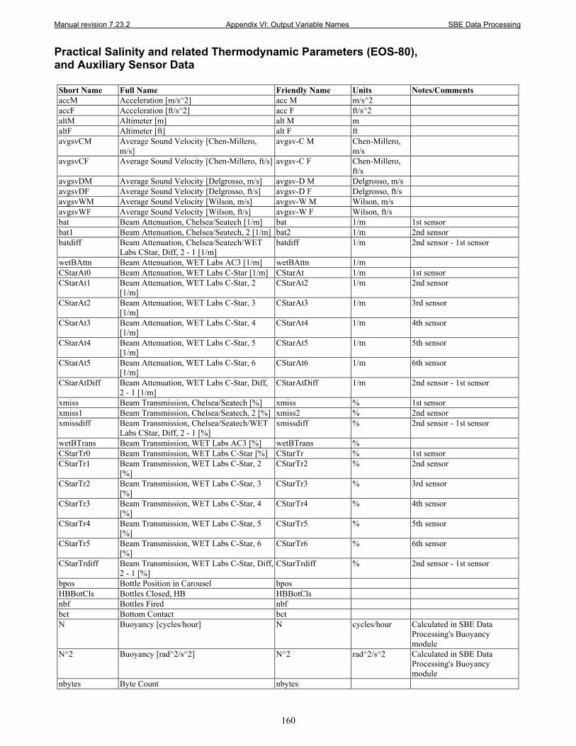
Manual revision 7.23.2 Appendix VI: Output Variable Names SBE Data Processing
160
Practical Salinity and related Thermodynamic Parameters (EOS-80), and Auxiliary Sensor Data
Short Name Full Name Friendly Name Units Notes/Comments accM Acceleration [m/s^2] acc M m/s^2 accF Acceleration [ft/s^2] acc F ft/s^2 altM Altimeter [m] alt M m altF Altimeter [ft] alt F ft avgsvCM Average Sound Velocity [Chen-Millero,
m/s] avgsv-C M Chen-Millero,
m/s
avgsvCF Average Sound Velocity [Chen-Millero, ft/s] avgsv-C F Chen-Millero, ft/s
avgsvDM Average Sound Velocity [Delgrosso, m/s] avgsv-D M Delgrosso, m/s avgsvDF Average Sound Velocity [Delgrosso, ft/s] avgsv-D F Delgrosso, ft/s avgsvWM Average Sound Velocity [Wilson, m/s] avgsv-W M Wilson, m/s avgsvWF Average Sound Velocity [Wilson, ft/s] avgsv-W F Wilson, ft/s bat Beam Attenuation, Chelsea/Seatech [1/m] bat 1/m 1st sensor bat1 Beam Attenuation, Chelsea/Seatech, 2 [1/m] bat2 1/m 2nd sensor batdiff Beam Attenuation, Chelsea/Seatech/WET
Labs CStar, Diff, 2 - 1 [1/m] batdiff 1/m 2nd sensor - 1st sensor
wetBAttn Beam Attenuation, WET Labs AC3 [1/m] wetBAttn 1/m CStarAt0 Beam Attenuation, WET Labs C-Star [1/m] CStarAt 1/m 1st sensor CStarAt1 Beam Attenuation, WET Labs C-Star, 2
[1/m] CStarAt2 1/m 2nd sensor
CStarAt2 Beam Attenuation, WET Labs C-Star, 3 [1/m]
CStarAt3 1/m 3rd sensor
CStarAt3 Beam Attenuation, WET Labs C-Star, 4 [1/m]
CStarAt4 1/m 4th sensor
CStarAt4 Beam Attenuation, WET Labs C-Star, 5 [1/m]
CStarAt5 1/m 5th sensor
CStarAt5 Beam Attenuation, WET Labs C-Star, 6 [1/m]
CStarAt6 1/m 6th sensor
CStarAtDiff Beam Attenuation, WET Labs C-Star, Diff, 2 - 1 [1/m]
CStarAtDiff 1/m 2nd sensor - 1st sensor
xmiss Beam Transmission, Chelsea/Seatech [%] xmiss % 1st sensor xmiss1 Beam Transmission, Chelsea/Seatech, 2 [%] xmiss2 % 2nd sensor xmissdiff Beam Transmission, Chelsea/Seatech/WET
Labs CStar, Diff, 2 - 1 [%] xmissdiff % 2nd sensor - 1st sensor
wetBTrans Beam Transmission, WET Labs AC3 [%] wetBTrans % CStarTr0 Beam Transmission, WET Labs C-Star [%] CStarTr % 1st sensor CStarTr1 Beam Transmission, WET Labs C-Star, 2
[%] CStarTr2 % 2nd sensor
CStarTr2 Beam Transmission, WET Labs C-Star, 3 [%]
CStarTr3 % 3rd sensor
CStarTr3 Beam Transmission, WET Labs C-Star, 4 [%]
CStarTr4 % 4th sensor
CStarTr4 Beam Transmission, WET Labs C-Star, 5 [%]
CStarTr5 % 5th sensor
CStarTr5 Beam Transmission, WET Labs C-Star, 6 [%]
CStarTr6 % 6th sensor
CStarTrdiff Beam Transmission, WET Labs C-Star, Diff, 2 - 1 [%]
CStarTrdiff % 2nd sensor - 1st sensor
bpos Bottle Position in Carousel bpos HBBotCls Bottles Closed, HB HBBotCls nbf Bottles Fired nbf bct Bottom Contact bct N Buoyancy [cycles/hour] N cycles/hour Calculated in SBE Data
Processing's Buoyancy module
N^2 Buoyancy [rad^2/s^2] N^2 rad^2/s^2 Calculated in SBE Data Processing's Buoyancy module
nbytes Byte Count nbytes
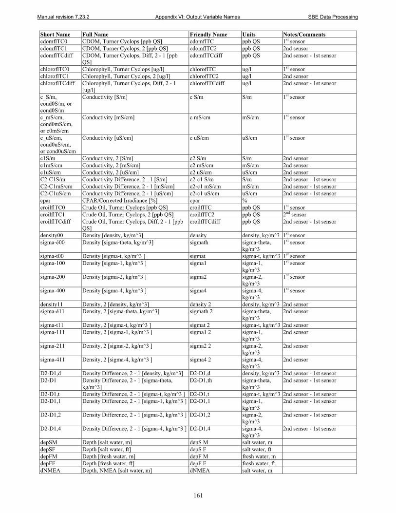
Manual revision 7.23.2 Appendix VI: Output Variable Names SBE Data Processing
161
Short Name Full Name Friendly Name Units Notes/Comments cdomflTC0 CDOM, Turner Cyclops [ppb QS] cdomflTC ppb QS 1st sensor cdomflTC1 CDOM, Turner Cyclops, 2 [ppb QS] cdomflTC2 ppb QS 2nd sensor cdomflTCdiff CDOM, Turner Cyclops, Diff, 2 - 1 [ppb
QS] cdomflTCdiff ppb QS 2nd sensor - 1st sensor
chloroflTC0 Chlorophyll, Turner Cyclops [ug/l] chloroflTC ug/l 1st sensor chloroflTC1 Chlorophyll, Turner Cyclops, 2 [ug/l] chloroflTC2 ug/l 2nd sensor chloroflTCdiff Chlorophyll, Turner Cyclops, Diff, 2 - 1
[ug/l] chloroflTCdiff ug/l 2nd sensor - 1st sensor
c_S/m, cond0S/m, or cond0S/m
Conductivity [S/m] c S/m S/m 1st sensor
c_mS/cm, cond0mS/cm, or c0mS/cm
Conductivity [mS/cm] c mS/cm mS/cm 1st sensor
c_uS/cm, cond0uS/cm, or cond0uS/cm
Conductivity [uS/cm] c uS/cm uS/cm 1st sensor
c1S/m Conductivity, 2 [S/m] c2 S/m S/m 2nd sensor c1mS/cm Conductivity, 2 [mS/cm] c2 mS/cm mS/cm 2nd sensor c1uS/cm Conductivity, 2 [uS/cm] c2 uS/cm uS/cm 2nd sensor C2-C1S/m Conductivity Difference, 2 - 1 [S/m] c2-c1 S/m S/m 2nd sensor - 1st sensor C2-C1mS/cm Conductivity Difference, 2 - 1 [mS/cm] c2-c1 mS/cm mS/cm 2nd sensor - 1st sensor C2-C1uS/cm Conductivity Difference, 2 - 1 [uS/cm] c2-c1 uS/cm uS/cm 2nd sensor - 1st sensor cpar CPAR/Corrected Irradiance [%] cpar % croilflTC0 Crude Oil, Turner Cyclops [ppb QS] croilflTC ppb QS 1st sensor croilflTC1 Crude Oil, Turner Cyclops, 2 [ppb QS] croilflTC2 ppb QS 2nd sensor croilflTCdiff Crude Oil, Turner Cyclops, Diff, 2 - 1 [ppb
QS] croilflTCdiff ppb QS 2nd sensor - 1st sensor
density00 Density [density, kg/m^3] density density, kg/m^3 1st sensor sigma-é00 Density [sigma-theta, kg/m^3] sigmath sigma-theta,
kg/m^3 1st sensor
sigma-t00 Density [sigma-t, kg/m^3 ] sigmat sigma-t, kg/m^3 1st sensor sigma-100 Density [sigma-1, kg/m^3 ] sigma1 sigma-1,
kg/m^3 1st sensor
sigma-200 Density [sigma-2, kg/m^3 ] sigma2 sigma-2, kg/m^3
1st sensor
sigma-400 Density [sigma-4, kg/m^3 ] sigma4 sigma-4, kg/m^3
1st sensor
density11 Density, 2 [density, kg/m^3] density 2 density, kg/m^3 2nd sensor sigma-é11 Density, 2 [sigma-theta, kg/m^3] sigmath 2 sigma-theta,
kg/m^3 2nd sensor
sigma-t11 Density, 2 [sigma-t, kg/m^3 ] sigmat 2 sigma-t, kg/m^3 2nd sensor sigma-111 Density, 2 [sigma-1, kg/m^3 ] sigma1 2 sigma-1,
kg/m^3 2nd sensor
sigma-211 Density, 2 [sigma-2, kg/m^3 ] sigma2 2 sigma-2, kg/m^3
2nd sensor
sigma-411 Density, 2 [sigma-4, kg/m^3 ] sigma4 2 sigma-4, kg/m^3
2nd sensor
D2-D1,d Density Difference, 2 - 1 [density, kg/m^3] D2-D1,d density, kg/m^3 2nd sensor - 1st sensor D2-D1 Density Difference, 2 - 1 [sigma-theta,
kg/m^3] D2-D1,th sigma-theta,
kg/m^3 2nd sensor - 1st sensor
D2-D1,t Density Difference, 2 - 1 [sigma-t, kg/m^3 ] D2-D1,t sigma-t, kg/m^3 2nd sensor - 1st sensor D2-D1,1 Density Difference, 2 - 1 [sigma-1, kg/m^3 ] D2-D1,1 sigma-1,
kg/m^3 2nd sensor - 1st sensor
D2-D1,2 Density Difference, 2 - 1 [sigma-2, kg/m^3 ] D2-D1,2 sigma-2, kg/m^3
2nd sensor - 1st sensor
D2-D1,4 Density Difference, 2 - 1 [sigma-4, kg/m^3 ] D2-D1,4 sigma-4, kg/m^3
2nd sensor - 1st sensor
depSM Depth [salt water, m] depS M salt water, m depSF Depth [salt water, ft] depS F salt water, ft depFM Depth [fresh water, m] depF M fresh water, m depFF Depth [fresh water, ft] depF F fresh water, ft dNMEA Depth, NMEA [salt water, m] dNMEA salt water, m
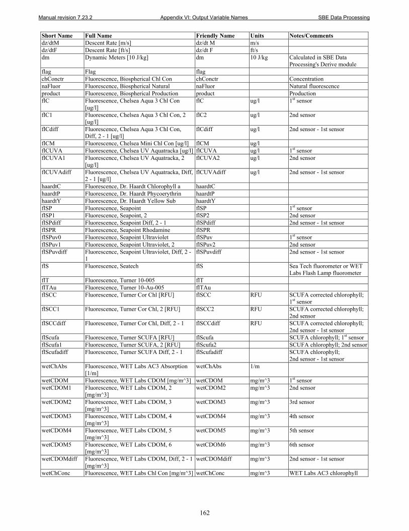
Manual revision 7.23.2 Appendix VI: Output Variable Names SBE Data Processing
162
Short Name Full Name Friendly Name Units Notes/Comments dz/dtM Descent Rate [m/s] dz/dt M m/s dz/dtF Descent Rate [ft/s] dz/dt F ft/s dm Dynamic Meters [10 J/kg] dm 10 J/kg Calculated in SBE Data
Processing's Derive module flag Flag flag chConctr Fluorescence, Biospherical Chl Con chConctr Concentration naFluor Fluorescence, Biospherical Natural naFluor Natural fluorescence product Fluorescence, Biospherical Production product Production flC Fluorescence, Chelsea Aqua 3 Chl Con
[ug/l] flC ug/l 1st sensor
flC1 Fluorescence, Chelsea Aqua 3 Chl Con, 2 [ug/l]
flC2 ug/l 2nd sensor
flCdiff Fluorescence, Chelsea Aqua 3 Chl Con, Diff, 2 - 1 [ug/l]
flCdiff ug/l 2nd sensor - 1st sensor
flCM Fluorescence, Chelsea Mini Chl Con [ug/l] flCM ug/l flCUVA Fluorescence, Chelsea UV Aquatracka [ug/l] flCUVA ug/l 1st sensor flCUVA1 Fluorescence, Chelsea UV Aquatracka, 2
[ug/l] flCUVA2 ug/l 2nd sensor
flCUVAdiff Fluorescence, Chelsea UV Aquatracka, Diff, 2 - 1 [ug/l]
flCUVAdiff ug/l 2nd sensor - 1st sensor
haardtC Fluorescence, Dr. Haardt Chlorophyll a haardtC haardtP Fluorescence, Dr. Haardt Phycoerythrin haardtP haardtY Fluorescence, Dr. Haardt Yellow Sub haardtY flSP Fluorescence, Seapoint flSP 1st sensor flSP1 Fluorescence, Seapoint, 2 flSP2 2nd sensor flSPdiff Fluorescence, Seapoint Diff, 2 - 1 flSPdiff 2nd sensor - 1st sensor flSPR Fluorescence, Seapoint Rhodamine flSPR flSPuv0 Fluorescence, Seapoint Ultraviolet flSPuv 1st sensor flSPuv1 Fluorescence, Seapoint Ultraviolet, 2 flSPuv2 2nd sensor flSPuvdiff Fluorescence, Seapoint Ultraviolet, Diff, 2 -
1 flSPuvdiff 2nd sensor - 1st sensor
flS Fluorescence, Seatech flS Sea Tech fluorometer or WET Labs Flash Lamp fluorometer
flT Fluorescence, Turner 10-005 flT flTAu Fluorescence, Turner 10-Au-005 flTAu flSCC Fluorescence, Turner Cor Chl [RFU] flSCC RFU SCUFA corrected chlorophyll;
1st sensor flSCC1 Fluorescence, Turner Cor Chl, 2 [RFU] flSCC2 RFU SCUFA corrected chlorophyll;
2nd sensor flSCCdiff Fluorescence, Turner Cor Chl, Diff, 2 - 1 flSCCdiff RFU SCUFA corrected chlorophyll;
2nd sensor - 1st sensor flScufa Fluorescence, Turner SCUFA [RFU] flScufa SCUFA chlorophyll; 1st sensor flScufa1 Fluorescence, Turner SCUFA, 2 [RFU] flScufa2 SCUFA chlorophyll; 2nd sensor flScufadiff Fluorescence, Turner SCUFA Diff, 2 - 1 flScufadiff SCUFA chlorophyll;
2nd sensor - 1st sensor wetChAbs Fluorescence, WET Labs AC3 Absorption
[1/m] wetChAbs 1/m
wetCDOM Fluorescence, WET Labs CDOM [mg/m^3] wetCDOM mg/m^3 1st sensor wetCDOM1 Fluorescence, WET Labs CDOM, 2
[mg/m^3] wetCDOM2 mg/m^3 2nd sensor
wetCDOM2 Fluorescence, WET Labs CDOM, 3 [mg/m^3]
wetCDOM3 mg/m^3 3rd sensor
wetCDOM3 Fluorescence, WET Labs CDOM, 4 [mg/m^3]
wetCDOM4 mg/m^3 4th sensor
wetCDOM4 Fluorescence, WET Labs CDOM, 5 [mg/m^3]
wetCDOM5 mg/m^3 5th sensor
wetCDOM5 Fluorescence, WET Labs CDOM, 6 [mg/m^3]
wetCDOM6 mg/m^3 6th sensor
wetCDOMdiff Fluorescence, WET Labs CDOM, Diff, 2 - 1 [mg/m^3]
wetCDOMdiff mg/m^3 2nd sensor - 1st sensor
wetChConc Fluorescence, WET Labs Chl Con [mg/m^3] wetChConc mg/m^3 WET Labs AC3 chlorophyll
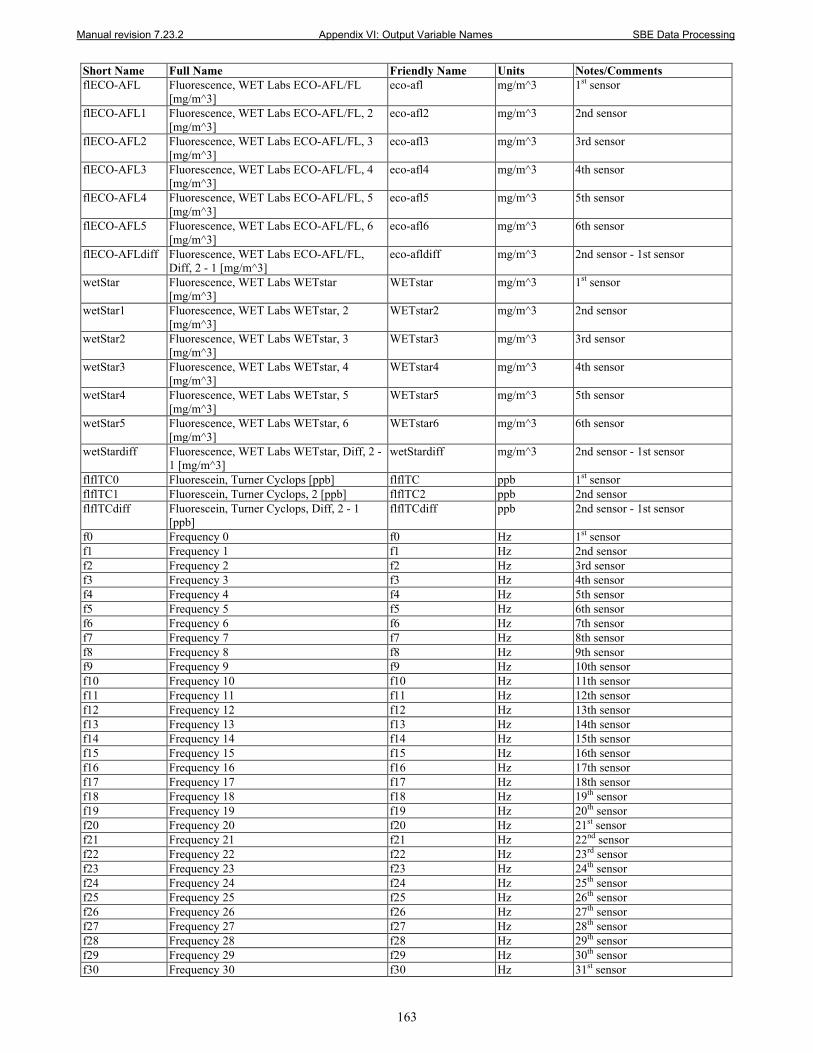
Manual revision 7.23.2 Appendix VI: Output Variable Names SBE Data Processing
163
Short Name Full Name Friendly Name Units Notes/Comments flECO-AFL Fluorescence, WET Labs ECO-AFL/FL
[mg/m^3] eco-afl mg/m^3 1st sensor
flECO-AFL1 Fluorescence, WET Labs ECO-AFL/FL, 2 [mg/m^3]
eco-afl2 mg/m^3 2nd sensor
flECO-AFL2 Fluorescence, WET Labs ECO-AFL/FL, 3 [mg/m^3]
eco-afl3 mg/m^3 3rd sensor
flECO-AFL3 Fluorescence, WET Labs ECO-AFL/FL, 4 [mg/m^3]
eco-afl4 mg/m^3 4th sensor
flECO-AFL4 Fluorescence, WET Labs ECO-AFL/FL, 5 [mg/m^3]
eco-afl5 mg/m^3 5th sensor
flECO-AFL5 Fluorescence, WET Labs ECO-AFL/FL, 6 [mg/m^3]
eco-afl6 mg/m^3 6th sensor
flECO-AFLdiff Fluorescence, WET Labs ECO-AFL/FL, Diff, 2 - 1 [mg/m^3]
eco-afldiff mg/m^3 2nd sensor - 1st sensor
wetStar Fluorescence, WET Labs WETstar [mg/m^3]
WETstar mg/m^3 1st sensor
wetStar1 Fluorescence, WET Labs WETstar, 2 [mg/m^3]
WETstar2 mg/m^3 2nd sensor
wetStar2 Fluorescence, WET Labs WETstar, 3 [mg/m^3]
WETstar3 mg/m^3 3rd sensor
wetStar3 Fluorescence, WET Labs WETstar, 4 [mg/m^3]
WETstar4 mg/m^3 4th sensor
wetStar4 Fluorescence, WET Labs WETstar, 5 [mg/m^3]
WETstar5 mg/m^3 5th sensor
wetStar5 Fluorescence, WET Labs WETstar, 6 [mg/m^3]
WETstar6 mg/m^3 6th sensor
wetStardiff Fluorescence, WET Labs WETstar, Diff, 2 - 1 [mg/m^3]
wetStardiff mg/m^3 2nd sensor - 1st sensor
flflTC0 Fluorescein, Turner Cyclops [ppb] flflTC ppb 1st sensor flflTC1 Fluorescein, Turner Cyclops, 2 [ppb] flflTC2 ppb 2nd sensor flflTCdiff Fluorescein, Turner Cyclops, Diff, 2 - 1
[ppb] flflTCdiff ppb 2nd sensor - 1st sensor
f0 Frequency 0 f0 Hz 1st sensor f1 Frequency 1 f1 Hz 2nd sensor f2 Frequency 2 f2 Hz 3rd sensor f3 Frequency 3 f3 Hz 4th sensor f4 Frequency 4 f4 Hz 5th sensor f5 Frequency 5 f5 Hz 6th sensor f6 Frequency 6 f6 Hz 7th sensor f7 Frequency 7 f7 Hz 8th sensor f8 Frequency 8 f8 Hz 9th sensor f9 Frequency 9 f9 Hz 10th sensor f10 Frequency 10 f10 Hz 11th sensor f11 Frequency 11 f11 Hz 12th sensor f12 Frequency 12 f12 Hz 13th sensor f13 Frequency 13 f13 Hz 14th sensor f14 Frequency 14 f14 Hz 15th sensor f15 Frequency 15 f15 Hz 16th sensor f16 Frequency 16 f16 Hz 17th sensor f17 Frequency 17 f17 Hz 18th sensor f18 Frequency 18 f18 Hz 19th sensor f19 Frequency 19 f19 Hz 20th sensor f20 Frequency 20 f20 Hz 21st sensor f21 Frequency 21 f21 Hz 22nd sensor f22 Frequency 22 f22 Hz 23rd sensor f23 Frequency 23 f23 Hz 24th sensor f24 Frequency 24 f24 Hz 25th sensor f25 Frequency 25 f25 Hz 26th sensor f26 Frequency 26 f26 Hz 27th sensor f27 Frequency 27 f27 Hz 28th sensor f28 Frequency 28 f28 Hz 29th sensor f29 Frequency 29 f29 Hz 30th sensor f30 Frequency 30 f30 Hz 31st sensor
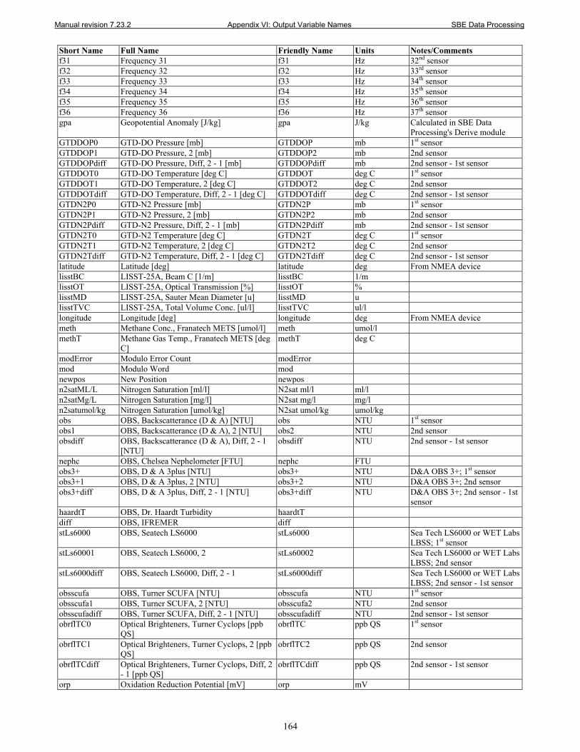
Manual revision 7.23.2 Appendix VI: Output Variable Names SBE Data Processing
164
Short Name Full Name Friendly Name Units Notes/Comments f31 Frequency 31 f31 Hz 32nd sensor f32 Frequency 32 f32 Hz 33rd sensor f33 Frequency 33 f33 Hz 34th sensor f34 Frequency 34 f34 Hz 35th sensor f35 Frequency 35 f35 Hz 36th sensor f36 Frequency 36 f36 Hz 37th sensor gpa Geopotential Anomaly [J/kg] gpa J/kg Calculated in SBE Data
Processing's Derive module GTDDOP0 GTD-DO Pressure [mb] GTDDOP mb 1st sensor GTDDOP1 GTD-DO Pressure, 2 [mb] GTDDOP2 mb 2nd sensor GTDDOPdiff GTD-DO Pressure, Diff, 2 - 1 [mb] GTDDOPdiff mb 2nd sensor - 1st sensor GTDDOT0 GTD-DO Temperature [deg C] GTDDOT deg C 1st sensor GTDDOT1 GTD-DO Temperature, 2 [deg C] GTDDOT2 deg C 2nd sensor GTDDOTdiff GTD-DO Temperature, Diff, 2 - 1 [deg C] GTDDOTdiff deg C 2nd sensor - 1st sensor GTDN2P0 GTD-N2 Pressure [mb] GTDN2P mb 1st sensor GTDN2P1 GTD-N2 Pressure, 2 [mb] GTDN2P2 mb 2nd sensor GTDN2Pdiff GTD-N2 Pressure, Diff, 2 - 1 [mb] GTDN2Pdiff mb 2nd sensor - 1st sensor GTDN2T0 GTD-N2 Temperature [deg C] GTDN2T deg C 1st sensor GTDN2T1 GTD-N2 Temperature, 2 [deg C] GTDN2T2 deg C 2nd sensor GTDN2Tdiff GTD-N2 Temperature, Diff, 2 - 1 [deg C] GTDN2Tdiff deg C 2nd sensor - 1st sensor latitude Latitude [deg] latitude deg From NMEA device lisstBC LISST-25A, Beam C [1/m] lisstBC 1/m lisstOT LISST-25A, Optical Transmission [%] lisstOT % lisstMD LISST-25A, Sauter Mean Diameter [u] lisstMD u lisstTVC LISST-25A, Total Volume Conc. [ul/l] lisstTVC ul/l longitude Longitude [deg] longitude deg From NMEA device meth Methane Conc., Franatech METS [umol/l] meth umol/l methT Methane Gas Temp., Franatech METS [deg
C] methT deg C
modError Modulo Error Count modError mod Modulo Word mod newpos New Position newpos n2satML/L Nitrogen Saturation [ml/l] N2sat ml/l ml/l n2satMg/L Nitrogen Saturation [mg/l] N2sat mg/l mg/l n2satumol/kg Nitrogen Saturation [umol/kg] N2sat umol/kg umol/kg obs OBS, Backscatterance (D & A) [NTU] obs NTU 1st sensor obs1 OBS, Backscatterance (D & A), 2 [NTU] obs2 NTU 2nd sensor obsdiff OBS, Backscatterance (D & A), Diff, 2 - 1
[NTU] obsdiff NTU 2nd sensor - 1st sensor
nephc OBS, Chelsea Nephelometer [FTU] nephc FTU obs3+ OBS, D & A 3plus [NTU] obs3+ NTU D&A OBS 3+; 1st sensor obs3+1 OBS, D & A 3plus, 2 [NTU] obs3+2 NTU D&A OBS 3+; 2nd sensor obs3+diff OBS, D & A 3plus, Diff, 2 - 1 [NTU] obs3+diff NTU D&A OBS 3+; 2nd sensor - 1st
sensor haardtT OBS, Dr. Haardt Turbidity haardtT diff OBS, IFREMER diff stLs6000 OBS, Seatech LS6000 stLs6000 Sea Tech LS6000 or WET Labs
LBSS; 1st sensor stLs60001 OBS, Seatech LS6000, 2 stLs60002 Sea Tech LS6000 or WET Labs
LBSS; 2nd sensor stLs6000diff OBS, Seatech LS6000, Diff, 2 - 1 stLs6000diff Sea Tech LS6000 or WET Labs
LBSS; 2nd sensor - 1st sensor obsscufa OBS, Turner SCUFA [NTU] obsscufa NTU 1st sensor obsscufa1 OBS, Turner SCUFA, 2 [NTU] obsscufa2 NTU 2nd sensor obsscufadiff OBS, Turner SCUFA, Diff, 2 - 1 [NTU] obsscufadiff NTU 2nd sensor - 1st sensor obrflTC0 Optical Brighteners, Turner Cyclops [ppb
QS] obrflTC ppb QS 1st sensor
obrflTC1 Optical Brighteners, Turner Cyclops, 2 [ppb QS]
obrflTC2 ppb QS 2nd sensor
obrflTCdiff Optical Brighteners, Turner Cyclops, Diff, 2 - 1 [ppb QS]
obrflTCdiff ppb QS 2nd sensor - 1st sensor
orp Oxidation Reduction Potential [mV] orp mV
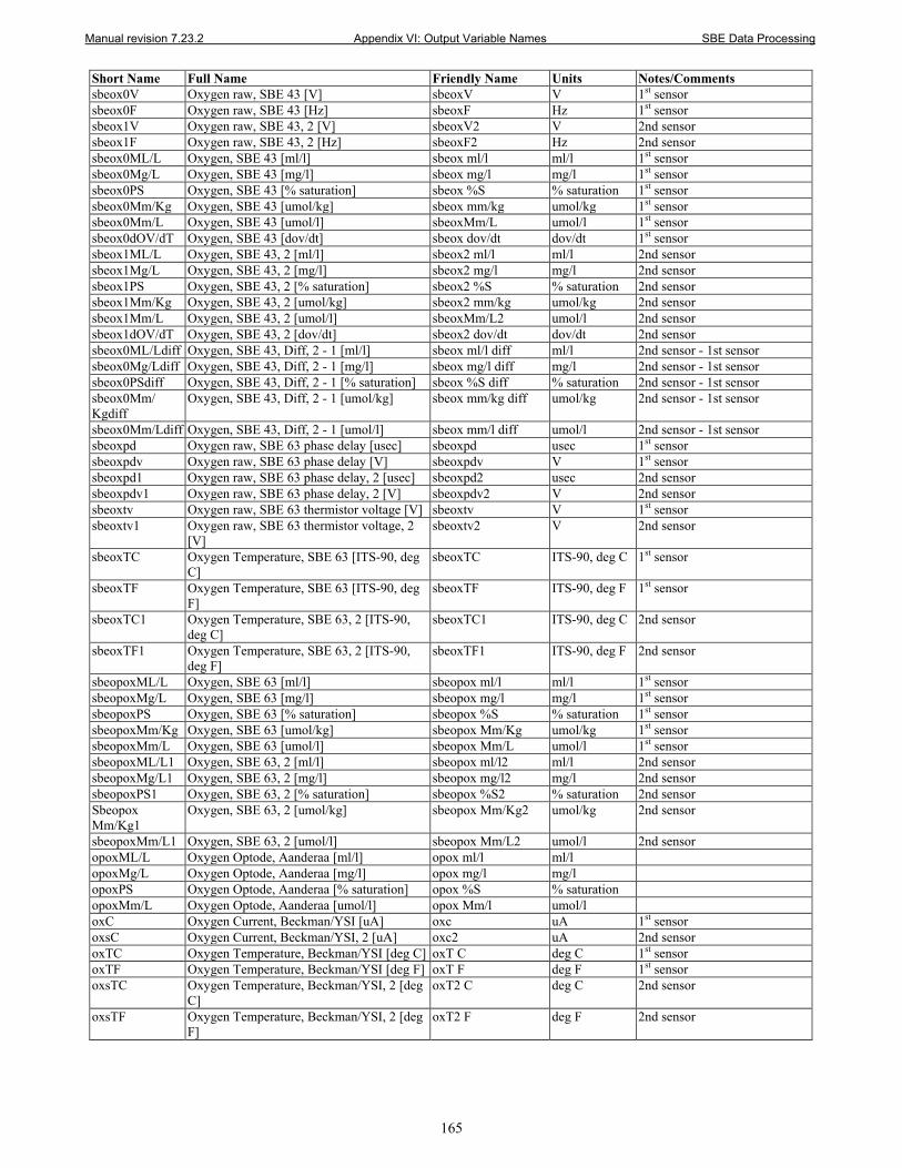
Manual revision 7.23.2 Appendix VI: Output Variable Names SBE Data Processing
165
Short Name Full Name Friendly Name Units Notes/Comments sbeox0V Oxygen raw, SBE 43 [V] sbeoxV V 1st sensor sbeox0F Oxygen raw, SBE 43 [Hz] sbeoxF Hz 1st sensor sbeox1V Oxygen raw, SBE 43, 2 [V] sbeoxV2 V 2nd sensor sbeox1F Oxygen raw, SBE 43, 2 [Hz] sbeoxF2 Hz 2nd sensor sbeox0ML/L Oxygen, SBE 43 [ml/l] sbeox ml/l ml/l 1st sensor sbeox0Mg/L Oxygen, SBE 43 [mg/l] sbeox mg/l mg/l 1st sensor sbeox0PS Oxygen, SBE 43 [% saturation] sbeox %S % saturation 1st sensor sbeox0Mm/Kg Oxygen, SBE 43 [umol/kg] sbeox mm/kg umol/kg 1st sensor sbeox0Mm/L Oxygen, SBE 43 [umol/l] sbeoxMm/L umol/l 1st sensor sbeox0dOV/dT Oxygen, SBE 43 [dov/dt] sbeox dov/dt dov/dt 1st sensor sbeox1ML/L Oxygen, SBE 43, 2 [ml/l] sbeox2 ml/l ml/l 2nd sensor sbeox1Mg/L Oxygen, SBE 43, 2 [mg/l] sbeox2 mg/l mg/l 2nd sensor sbeox1PS Oxygen, SBE 43, 2 [% saturation] sbeox2 %S % saturation 2nd sensor sbeox1Mm/Kg Oxygen, SBE 43, 2 [umol/kg] sbeox2 mm/kg umol/kg 2nd sensor sbeox1Mm/L Oxygen, SBE 43, 2 [umol/l] sbeoxMm/L2 umol/l 2nd sensor sbeox1dOV/dT Oxygen, SBE 43, 2 [dov/dt] sbeox2 dov/dt dov/dt 2nd sensor sbeox0ML/Ldiff Oxygen, SBE 43, Diff, 2 - 1 [ml/l] sbeox ml/l diff ml/l 2nd sensor - 1st sensor sbeox0Mg/Ldiff Oxygen, SBE 43, Diff, 2 - 1 [mg/l] sbeox mg/l diff mg/l 2nd sensor - 1st sensor sbeox0PSdiff Oxygen, SBE 43, Diff, 2 - 1 [% saturation] sbeox %S diff % saturation 2nd sensor - 1st sensor sbeox0Mm/ Kgdiff
Oxygen, SBE 43, Diff, 2 - 1 [umol/kg] sbeox mm/kg diff umol/kg 2nd sensor - 1st sensor
sbeox0Mm/Ldiff Oxygen, SBE 43, Diff, 2 - 1 [umol/l] sbeox mm/l diff umol/l 2nd sensor - 1st sensor sbeoxpd Oxygen raw, SBE 63 phase delay [usec] sbeoxpd usec 1st sensor sbeoxpdv Oxygen raw, SBE 63 phase delay [V] sbeoxpdv V 1st sensor sbeoxpd1 Oxygen raw, SBE 63 phase delay, 2 [usec] sbeoxpd2 usec 2nd sensor sbeoxpdv1 Oxygen raw, SBE 63 phase delay, 2 [V] sbeoxpdv2 V 2nd sensor sbeoxtv Oxygen raw, SBE 63 thermistor voltage [V] sbeoxtv V 1st sensor sbeoxtv1 Oxygen raw, SBE 63 thermistor voltage, 2
[V] sbeoxtv2 V 2nd sensor
sbeoxTC Oxygen Temperature, SBE 63 [ITS-90, deg C]
sbeoxTC ITS-90, deg C 1st sensor
sbeoxTF Oxygen Temperature, SBE 63 [ITS-90, deg F]
sbeoxTF ITS-90, deg F 1st sensor
sbeoxTC1 Oxygen Temperature, SBE 63, 2 [ITS-90, deg C]
sbeoxTC1 ITS-90, deg C 2nd sensor
sbeoxTF1 Oxygen Temperature, SBE 63, 2 [ITS-90, deg F]
sbeoxTF1 ITS-90, deg F 2nd sensor
sbeopoxML/L Oxygen, SBE 63 [ml/l] sbeopox ml/l ml/l 1st sensor sbeopoxMg/L Oxygen, SBE 63 [mg/l] sbeopox mg/l mg/l 1st sensor sbeopoxPS Oxygen, SBE 63 [% saturation] sbeopox %S % saturation 1st sensor sbeopoxMm/Kg Oxygen, SBE 63 [umol/kg] sbeopox Mm/Kg umol/kg 1st sensor sbeopoxMm/L Oxygen, SBE 63 [umol/l] sbeopox Mm/L umol/l 1st sensor sbeopoxML/L1 Oxygen, SBE 63, 2 [ml/l] sbeopox ml/l2 ml/l 2nd sensor sbeopoxMg/L1 Oxygen, SBE 63, 2 [mg/l] sbeopox mg/l2 mg/l 2nd sensor sbeopoxPS1 Oxygen, SBE 63, 2 [% saturation] sbeopox %S2 % saturation 2nd sensor Sbeopox Mm/Kg1
Oxygen, SBE 63, 2 [umol/kg] sbeopox Mm/Kg2 umol/kg 2nd sensor
sbeopoxMm/L1 Oxygen, SBE 63, 2 [umol/l] sbeopox Mm/L2 umol/l 2nd sensor opoxML/L Oxygen Optode, Aanderaa [ml/l] opox ml/l ml/l opoxMg/L Oxygen Optode, Aanderaa [mg/l] opox mg/l mg/l opoxPS Oxygen Optode, Aanderaa [% saturation] opox %S % saturation opoxMm/L Oxygen Optode, Aanderaa [umol/l] opox Mm/l umol/l oxC Oxygen Current, Beckman/YSI [uA] oxc uA 1st sensor oxsC Oxygen Current, Beckman/YSI, 2 [uA] oxc2 uA 2nd sensor oxTC Oxygen Temperature, Beckman/YSI [deg C] oxT C deg C 1st sensor oxTF Oxygen Temperature, Beckman/YSI [deg F] oxT F deg F 1st sensor oxsTC Oxygen Temperature, Beckman/YSI, 2 [deg
C] oxT2 C deg C 2nd sensor
oxsTF Oxygen Temperature, Beckman/YSI, 2 [deg F]
oxT2 F deg F 2nd sensor
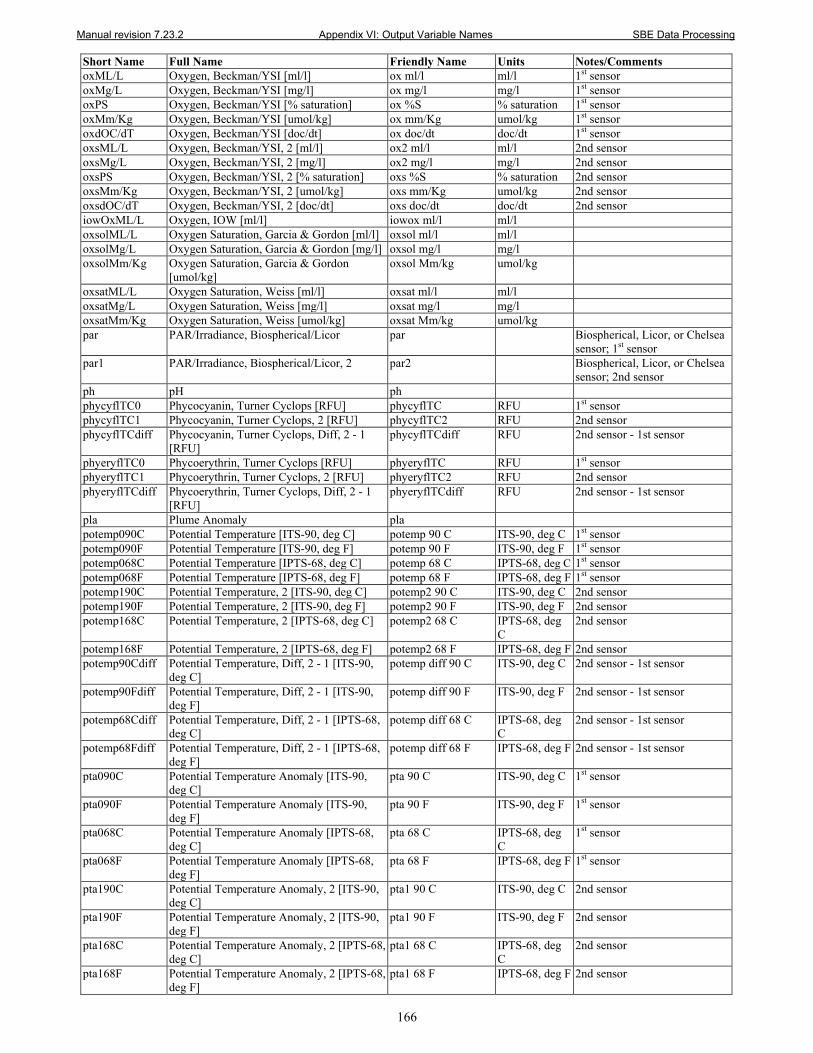
Manual revision 7.23.2 Appendix VI: Output Variable Names SBE Data Processing
166
Short Name Full Name Friendly Name Units Notes/Comments oxML/L Oxygen, Beckman/YSI [ml/l] ox ml/l ml/l 1st sensor oxMg/L Oxygen, Beckman/YSI [mg/l] ox mg/l mg/l 1st sensor oxPS Oxygen, Beckman/YSI [% saturation] ox %S % saturation 1st sensor oxMm/Kg Oxygen, Beckman/YSI [umol/kg] ox mm/Kg umol/kg 1st sensor oxdOC/dT Oxygen, Beckman/YSI [doc/dt] ox doc/dt doc/dt 1st sensor oxsML/L Oxygen, Beckman/YSI, 2 [ml/l] ox2 ml/l ml/l 2nd sensor oxsMg/L Oxygen, Beckman/YSI, 2 [mg/l] ox2 mg/l mg/l 2nd sensor oxsPS Oxygen, Beckman/YSI, 2 [% saturation] oxs %S % saturation 2nd sensor oxsMm/Kg Oxygen, Beckman/YSI, 2 [umol/kg] oxs mm/Kg umol/kg 2nd sensor oxsdOC/dT Oxygen, Beckman/YSI, 2 [doc/dt] oxs doc/dt doc/dt 2nd sensor iowOxML/L Oxygen, IOW [ml/l] iowox ml/l ml/l oxsolML/L Oxygen Saturation, Garcia & Gordon [ml/l] oxsol ml/l ml/l oxsolMg/L Oxygen Saturation, Garcia & Gordon [mg/l] oxsol mg/l mg/l oxsolMm/Kg Oxygen Saturation, Garcia & Gordon
[umol/kg] oxsol Mm/kg umol/kg
oxsatML/L Oxygen Saturation, Weiss [ml/l] oxsat ml/l ml/l oxsatMg/L Oxygen Saturation, Weiss [mg/l] oxsat mg/l mg/l oxsatMm/Kg Oxygen Saturation, Weiss [umol/kg] oxsat Mm/kg umol/kg par PAR/Irradiance, Biospherical/Licor par Biospherical, Licor, or Chelsea
sensor; 1st sensor par1 PAR/Irradiance, Biospherical/Licor, 2 par2 Biospherical, Licor, or Chelsea
sensor; 2nd sensor ph pH ph phycyflTC0 Phycocyanin, Turner Cyclops [RFU] phycyflTC RFU 1st sensor phycyflTC1 Phycocyanin, Turner Cyclops, 2 [RFU] phycyflTC2 RFU 2nd sensor phycyflTCdiff Phycocyanin, Turner Cyclops, Diff, 2 - 1
[RFU] phycyflTCdiff RFU 2nd sensor - 1st sensor
phyeryflTC0 Phycoerythrin, Turner Cyclops [RFU] phyeryflTC RFU 1st sensor phyeryflTC1 Phycoerythrin, Turner Cyclops, 2 [RFU] phyeryflTC2 RFU 2nd sensor phyeryflTCdiff Phycoerythrin, Turner Cyclops, Diff, 2 - 1
[RFU] phyeryflTCdiff RFU 2nd sensor - 1st sensor
pla Plume Anomaly pla potemp090C Potential Temperature [ITS-90, deg C] potemp 90 C ITS-90, deg C 1st sensor potemp090F Potential Temperature [ITS-90, deg F] potemp 90 F ITS-90, deg F 1st sensor potemp068C Potential Temperature [IPTS-68, deg C] potemp 68 C IPTS-68, deg C 1st sensor potemp068F Potential Temperature [IPTS-68, deg F] potemp 68 F IPTS-68, deg F 1st sensor potemp190C Potential Temperature, 2 [ITS-90, deg C] potemp2 90 C ITS-90, deg C 2nd sensor potemp190F Potential Temperature, 2 [ITS-90, deg F] potemp2 90 F ITS-90, deg F 2nd sensor potemp168C Potential Temperature, 2 [IPTS-68, deg C] potemp2 68 C IPTS-68, deg
C 2nd sensor
potemp168F Potential Temperature, 2 [IPTS-68, deg F] potemp2 68 F IPTS-68, deg F 2nd sensor potemp90Cdiff Potential Temperature, Diff, 2 - 1 [ITS-90,
deg C] potemp diff 90 C ITS-90, deg C 2nd sensor - 1st sensor
potemp90Fdiff Potential Temperature, Diff, 2 - 1 [ITS-90, deg F]
potemp diff 90 F ITS-90, deg F 2nd sensor - 1st sensor
potemp68Cdiff Potential Temperature, Diff, 2 - 1 [IPTS-68, deg C]
potemp diff 68 C IPTS-68, deg C
2nd sensor - 1st sensor
potemp68Fdiff Potential Temperature, Diff, 2 - 1 [IPTS-68, deg F]
potemp diff 68 F IPTS-68, deg F 2nd sensor - 1st sensor
pta090C Potential Temperature Anomaly [ITS-90, deg C]
pta 90 C ITS-90, deg C 1st sensor
pta090F Potential Temperature Anomaly [ITS-90, deg F]
pta 90 F ITS-90, deg F 1st sensor
pta068C Potential Temperature Anomaly [IPTS-68, deg C]
pta 68 C IPTS-68, deg C
1st sensor
pta068F Potential Temperature Anomaly [IPTS-68, deg F]
pta 68 F IPTS-68, deg F 1st sensor
pta190C Potential Temperature Anomaly, 2 [ITS-90, deg C]
pta1 90 C ITS-90, deg C 2nd sensor
pta190F Potential Temperature Anomaly, 2 [ITS-90, deg F]
pta1 90 F ITS-90, deg F 2nd sensor
pta168C Potential Temperature Anomaly, 2 [IPTS-68, deg C]
pta1 68 C IPTS-68, deg C
2nd sensor
pta168F Potential Temperature Anomaly, 2 [IPTS-68, deg F]
pta1 68 F IPTS-68, deg F 2nd sensor
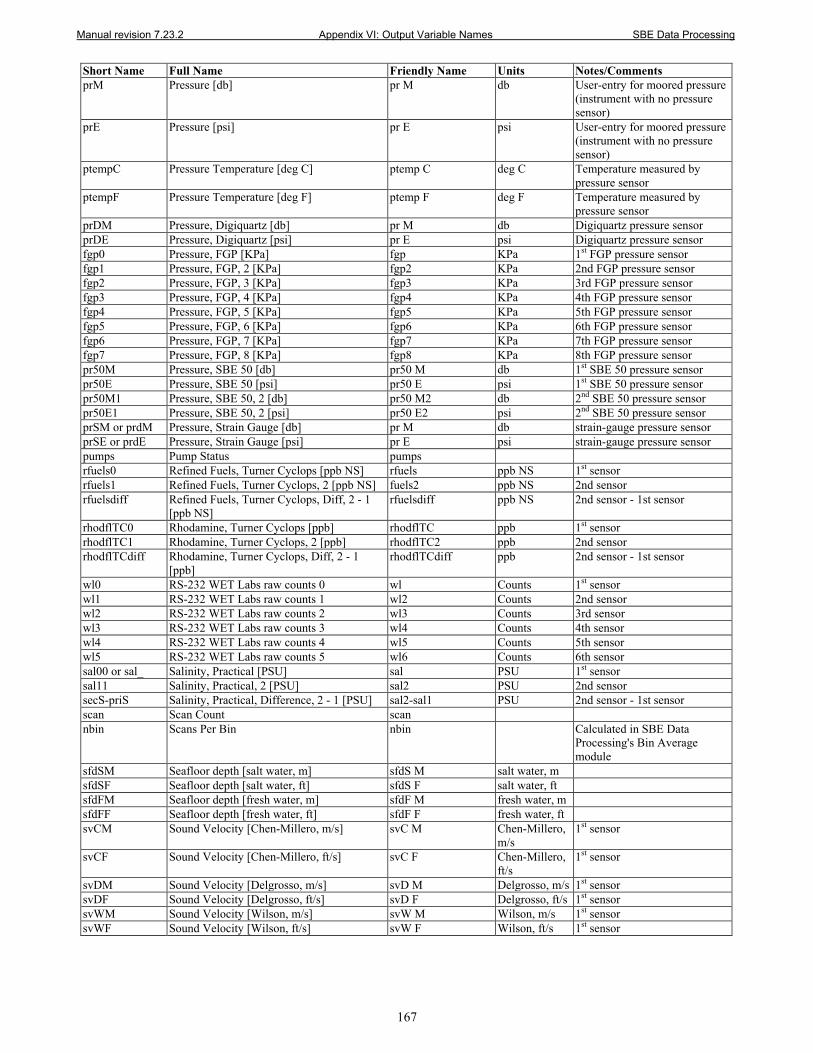
Manual revision 7.23.2 Appendix VI: Output Variable Names SBE Data Processing
167
Short Name Full Name Friendly Name Units Notes/Comments prM Pressure [db] pr M db User-entry for moored pressure
(instrument with no pressure sensor)
prE Pressure [psi] pr E psi User-entry for moored pressure (instrument with no pressure sensor)
ptempC Pressure Temperature [deg C] ptemp C deg C Temperature measured by pressure sensor
ptempF Pressure Temperature [deg F] ptemp F deg F Temperature measured by pressure sensor
prDM Pressure, Digiquartz [db] pr M db Digiquartz pressure sensor prDE Pressure, Digiquartz [psi] pr E psi Digiquartz pressure sensor fgp0 Pressure, FGP [KPa] fgp KPa 1st FGP pressure sensor fgp1 Pressure, FGP, 2 [KPa] fgp2 KPa 2nd FGP pressure sensor fgp2 Pressure, FGP, 3 [KPa] fgp3 KPa 3rd FGP pressure sensor fgp3 Pressure, FGP, 4 [KPa] fgp4 KPa 4th FGP pressure sensor fgp4 Pressure, FGP, 5 [KPa] fgp5 KPa 5th FGP pressure sensor fgp5 Pressure, FGP, 6 [KPa] fgp6 KPa 6th FGP pressure sensor fgp6 Pressure, FGP, 7 [KPa] fgp7 KPa 7th FGP pressure sensor fgp7 Pressure, FGP, 8 [KPa] fgp8 KPa 8th FGP pressure sensor pr50M Pressure, SBE 50 [db] pr50 M db 1st SBE 50 pressure sensor pr50E Pressure, SBE 50 [psi] pr50 E psi 1st SBE 50 pressure sensor pr50M1 Pressure, SBE 50, 2 [db] pr50 M2 db 2nd SBE 50 pressure sensor pr50E1 Pressure, SBE 50, 2 [psi] pr50 E2 psi 2nd SBE 50 pressure sensor prSM or prdM Pressure, Strain Gauge [db] pr M db strain-gauge pressure sensor prSE or prdE Pressure, Strain Gauge [psi] pr E psi strain-gauge pressure sensor pumps Pump Status pumps rfuels0 Refined Fuels, Turner Cyclops [ppb NS] rfuels ppb NS 1st sensor rfuels1 Refined Fuels, Turner Cyclops, 2 [ppb NS] fuels2 ppb NS 2nd sensor rfuelsdiff Refined Fuels, Turner Cyclops, Diff, 2 - 1
[ppb NS] rfuelsdiff ppb NS 2nd sensor - 1st sensor
rhodflTC0 Rhodamine, Turner Cyclops [ppb] rhodflTC ppb 1st sensor rhodflTC1 Rhodamine, Turner Cyclops, 2 [ppb] rhodflTC2 ppb 2nd sensor rhodflTCdiff Rhodamine, Turner Cyclops, Diff, 2 - 1
[ppb] rhodflTCdiff ppb 2nd sensor - 1st sensor
wl0 RS-232 WET Labs raw counts 0 wl Counts 1st sensor wl1 RS-232 WET Labs raw counts 1 wl2 Counts 2nd sensor wl2 RS-232 WET Labs raw counts 2 wl3 Counts 3rd sensor wl3 RS-232 WET Labs raw counts 3 wl4 Counts 4th sensor wl4 RS-232 WET Labs raw counts 4 wl5 Counts 5th sensor wl5 RS-232 WET Labs raw counts 5 wl6 Counts 6th sensor sal00 or sal_ Salinity, Practical [PSU] sal PSU 1st sensor sal11 Salinity, Practical, 2 [PSU] sal2 PSU 2nd sensor secS-priS Salinity, Practical, Difference, 2 - 1 [PSU] sal2-sal1 PSU 2nd sensor - 1st sensor scan Scan Count scan nbin Scans Per Bin nbin Calculated in SBE Data
Processing's Bin Average module
sfdSM Seafloor depth [salt water, m] sfdS M salt water, m sfdSF Seafloor depth [salt water, ft] sfdS F salt water, ft sfdFM Seafloor depth [fresh water, m] sfdF M fresh water, m sfdFF Seafloor depth [fresh water, ft] sfdF F fresh water, ft svCM Sound Velocity [Chen-Millero, m/s] svC M Chen-Millero,
m/s 1st sensor
svCF Sound Velocity [Chen-Millero, ft/s] svC F Chen-Millero, ft/s
1st sensor
svDM Sound Velocity [Delgrosso, m/s] svD M Delgrosso, m/s 1st sensor svDF Sound Velocity [Delgrosso, ft/s] svD F Delgrosso, ft/s 1st sensor svWM Sound Velocity [Wilson, m/s] svW M Wilson, m/s 1st sensor svWF Sound Velocity [Wilson, ft/s] svW F Wilson, ft/s 1st sensor
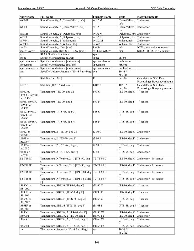
Manual revision 7.23.2 Appendix VI: Output Variable Names SBE Data Processing
168
Short Name Full Name Friendly Name Units Notes/Comments svCM1 Sound Velocity, 2 [Chen-Millero, m/s] svC2 M Chen-Millero,
m/s 2nd sensor
svCF1 Sound Velocity, 2 [Chen-Millero, ft/s] svC2 F Chen-Millero, ft/s
2nd sensor
svDM1 Sound Velocity, 2 [Delgrosso, m/s] svD2 M Delgrosso, m/s 2nd sensor svDF1 Sound Velocity, 2 [Delgrosso, ft/s] svD2 F Delgrosso, ft/s 2nd sensor svWM1 Sound Velocity, 2 [Wilson, m/s] svW2 M Wilson, m/s 2nd sensor svWF1 Sound Velocity, 2 [Wilson, ft/s] svW2 F Wilson, ft/s 2nd sensor iowSv Sound Velocity, IOW [m/s] iowSv m/s IOW sound velocity sensor sbeSv-iowSv Sound Velocity Diff, SBE - IOW [m/s] svSbeC-svIOW m/s SBE CTD - IOW SV sensor spar SPAR/Surface Irradiance spar specc Specific Conductance [uS/cm] specc uS/cm speccumhoscm Specific Conductance [umhos/cm] speccumhoscm umhos/cm speccmsm Specific Conductance [mS/cm] speccmsm mS/cm speccmmhoscm Specific Conductance [mmhos/cm] speccmmhoscm mmhos/cm sva Specific Volume Anomaly [10^-8 * m^3/kg] sva 10^-8 *
m^3/kg
E Stability [rad^2/m] E rad^2/m Calculated in SBE Data Processing's Buoyancy module
E10^-8 Stability [10^-8 * rad^2/m] E10^-8 10^-8 * rad^2/m
Calculated in SBE Data Processing's Buoyancy module
t090Cm, t4990C, tnc90C, or tv290C
Temperature [ITS-90, deg C] t 90 C ITS-90, deg C 1st sensor
t090F, t4990F, tnc90F, or tv290F
Temperature [ITS-90, deg F] t 90 F ITS-90, deg F 1st sensor
t068C, t4968C, tnc68C, or tv268C
Temperature [IPTS-68, deg C] t 68 C IPTS-68, deg C
1st sensor
t068F, t4968F, tnc68F, or tv268F
Temperature [IPTS-68, deg F] t 68 F IPTS-68, deg F 1st sensor
t190C or tnc290C
Temperature, 2 [ITS-90, deg C] t2 90 C ITS-90, deg C 2nd sensor
t190F or tnc290F
Temperature, 2 [ITS-90, deg F] t2 90 F ITS-90, deg F 2nd sensor
t168C or tnc268C
Temperature, 2 [IPTS-68, deg C] t2 68 C IPTS-68, deg C
2nd sensor
t168F or tnc268F
Temperature, 2 [IPTS-68, deg F] t2 68 F IPTS-68, deg F 2nd sensor
T2-T190C Temperature Difference, 2 - 1 [ITS-90, deg C]
T2-T1 90 C ITS-90, deg C 2nd sensor - 1st sensor
T2-T190F Temperature Difference, 2 - 1 [ITS-90, deg F]
T2-T1 90 F ITS-90, deg F 2nd sensor - 1st sensor
T2-T168C Temperature Difference, 2 - 1 [IPTS-68, deg C]
T2-T1 68 C IPTS-68, deg C
2nd sensor - 1st sensor
T2-T168F Temperature Difference, 2 - 1 [IPTS-68, deg F]
T2-T1 68 F IPTS-68, deg F 2nd sensor - 1st sensor
t3890C or t38_90C
Temperature, SBE 38 [ITS-90, deg C] t38 90 C ITS-90, deg C 1st sensor
t3890F or t38_90F
Temperature, SBE 38 [ITS-90, deg F] t38 90 F ITS-90, deg F 1st sensor
t3868C or t38_68C
Temperature, SBE 38 [IPTS-68, deg C] t38 68 C IPTS-68, deg C
1st sensor
t3868F or t38_68F
Temperature, SBE 38 [IPTS-68, deg F] t38 68 F IPTS-68, deg F 1st sensor
t3890C1 Temperature, SBE 38, 2 [ITS-90, deg C] t38 90 C2 ITS-90, deg C 2nd sensor t3890F1 Temperature, SBE 38, 2 [ITS-90, deg F] t38 90 F2 ITS-90, deg F 2nd sensor t3868C1 Temperature, SBE 38, 2 [IPTS-68, deg C] t38 68 C2 IPTS-68, deg
C 2nd sensor
t3868F1 Temperature, SBE 38, 2 [IPTS-68, deg F] t38 68 F2 IPTS-68, deg F 2nd sensor tsa Thermosteric Anomaly [10^-8 * m^3/kg] tsa 10^-8 *
m^3/kg
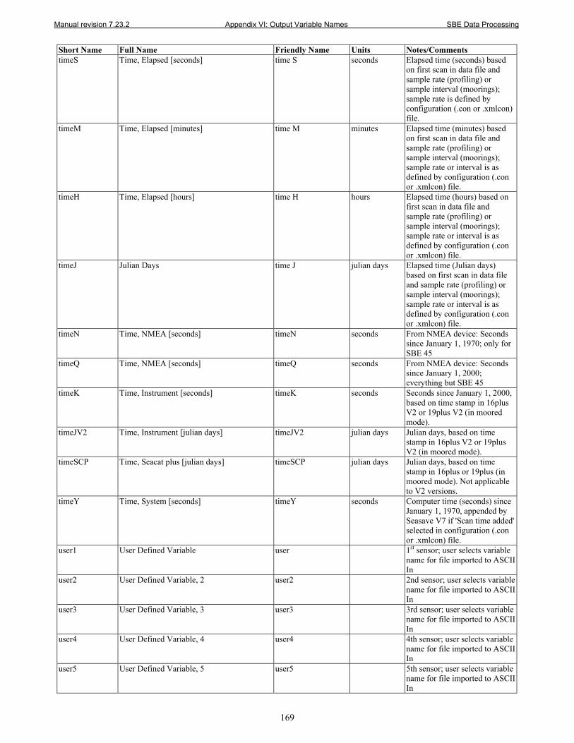
Manual revision 7.23.2 Appendix VI: Output Variable Names SBE Data Processing
169
Short Name Full Name Friendly Name Units Notes/Comments timeS Time, Elapsed [seconds] time S seconds Elapsed time (seconds) based
on first scan in data file and sample rate (profiling) or sample interval (moorings); sample rate is defined by configuration (.con or .xmlcon) file.
timeM Time, Elapsed [minutes] time M minutes Elapsed time (minutes) based on first scan in data file and sample rate (profiling) or sample interval (moorings); sample rate or interval is as defined by configuration (.con or .xmlcon) file.
timeH Time, Elapsed [hours] time H hours Elapsed time (hours) based on first scan in data file and sample rate (profiling) or sample interval (moorings); sample rate or interval is as defined by configuration (.con or .xmlcon) file.
timeJ Julian Days time J julian days Elapsed time (Julian days) based on first scan in data file and sample rate (profiling) or sample interval (moorings); sample rate or interval is as defined by configuration (.con or .xmlcon) file.
timeN Time, NMEA [seconds] timeN seconds From NMEA device: Seconds since January 1, 1970; only for SBE 45
timeQ Time, NMEA [seconds] timeQ seconds From NMEA device: Seconds since January 1, 2000; everything but SBE 45
timeK Time, Instrument [seconds] timeK seconds Seconds since January 1, 2000, based on time stamp in 16plus V2 or 19plus V2 (in moored mode).
timeJV2 Time, Instrument [julian days] timeJV2 julian days Julian days, based on time stamp in 16plus V2 or 19plus V2 (in moored mode).
timeSCP Time, Seacat plus [julian days] timeSCP julian days Julian days, based on time stamp in 16plus or 19plus (in moored mode). Not applicable to V2 versions.
timeY Time, System [seconds] timeY seconds Computer time (seconds) since January 1, 1970, appended by Seasave V7 if 'Scan time added' selected in configuration (.con or .xmlcon) file.
user1 User Defined Variable user 1st sensor; user selects variable name for file imported to ASCII In
user2 User Defined Variable, 2 user2 2nd sensor; user selects variable name for file imported to ASCII In
user3 User Defined Variable, 3 user3 3rd sensor; user selects variable name for file imported to ASCII In
user4 User Defined Variable, 4 user4 4th sensor; user selects variable name for file imported to ASCII In
user5 User Defined Variable, 5 user5 5th sensor; user selects variable name for file imported to ASCII In
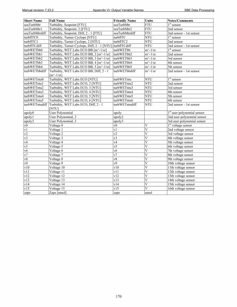
Manual revision 7.23.2 Appendix VI: Output Variable Names SBE Data Processing
170
Short Name Full Name Friendly Name Units Notes/Comments seaTurbMtr Turbidity, Seapoint [FTU] seaTurbMtr FTU 1st sensor seaTurbMtr1 Turbidity, Seapoint, 2 [FTU] seaTurbMtr2 FTU 2nd sensor seaTurbMtrdiff Turbidity, Seapoint, Diff, 2 - 1 [FTU] seaTurbMtrdiff FTU 2nd sensor - 1st sensor turbflTC0 Turbidity, Turner Cyclops [NTU] turbflTC NTU 1st sensor turbflTC1 Turbidity, Turner Cyclops, 2 [NTU] turbflTC2 NTU 2nd sensor turbflTCdiff Turbidity, Turner Cyclops, Diff, 2 - 1 [NTU] turbflTCdiff NTU 2nd sensor - 1st sensor turbWETbb0 Turbidity, WET Labs ECO BB [m^-1/sr] turbWETbb m^-1/sr 1st sensor turbWETbb1 Turbidity, WET Labs ECO BB, 2 [m^-1/sr] turbWETbb2 m^-1/sr 2nd sensor turbWETbb2 Turbidity, WET Labs ECO BB, 3 [m^-1/sr] turbWETbb3 m^-1/sr 3rd sensor turbWETbb3 Turbidity, WET Labs ECO BB, 4 [m^-1/sr] turbWETbb4 m^-1/sr 4th sensor turbWETbb4 Turbidity, WET Labs ECO BB, 5 [m^-1/sr] turbWETbb5 m^-1/sr 5th sensor turbWETbbdiff Turbidity, WET Labs ECO BB, Diff, 2 - 1
[m^-1/sr] turbWETbbdiff m^-1/sr 2nd sensor - 1st sensor
turbWETntu0 Turbidity, WET Labs ECO [NTU] turbWETntu NTU 1st sensor turbWETntu1 Turbidity, WET Labs ECO, 2 [NTU] turbWETntu2 NTU 2nd sensor turbWETntu2 Turbidity, WET Labs ECO, 3 [NTU] turbWETntu3 NTU 3rd sensor turbWETntu3 Turbidity, WET Labs ECO, 4 [NTU] turbWETntu4 NTU 4th sensor turbWETntu4 Turbidity, WET Labs ECO, 5 [NTU] turbWETntu5 NTU 5th sensor turbWETntu5 Turbidity, WET Labs ECO, 6 [NTU] turbWETntu6 NTU 6th sensor turbWETntudiff Turbidity, WET Labs ECO, Diff, 2 - 1
[NTU] turbWETntudiff NTU 2nd sensor - 1st sensor
upoly0 User Polynomial upoly 1st user polynomial sensor upoly1 User Polynomial, 2 upoly2 2nd user polynomial sensor upoly2 User Polynomial, 3 upoly3 3rd user polynomial sensor v0 Voltage 0 v0 V 1st voltage sensor v1 Voltage 1 v1 V 2nd voltage sensor v2 Voltage 2 v2 V 3rd voltage sensor v3 Voltage 3 v3 V 4th voltage sensor v4 Voltage 4 v4 V 5th voltage sensor v5 Voltage 5 v5 V 6th voltage sensor v6 Voltage 6 v6 V 7th voltage sensor v7 Voltage 7 v7 V 8th voltage sensor v8 Voltage 8 v8 V 9th voltage sensor v9 Voltage 9 v9 V 10th voltage sensor v10 Voltage 10 v10 V 11th voltage sensor v11 Voltage 11 v11 V 12th voltage sensor v12 Voltage 12 v12 V 13th voltage sensor v13 Voltage 13 v13 V 14th voltage sensor v14 Voltage 14 v14 V 15th voltage sensor v15 Voltage 15 v15 V 16th voltage sensor zaps Zaps [nmol] zaps nmol
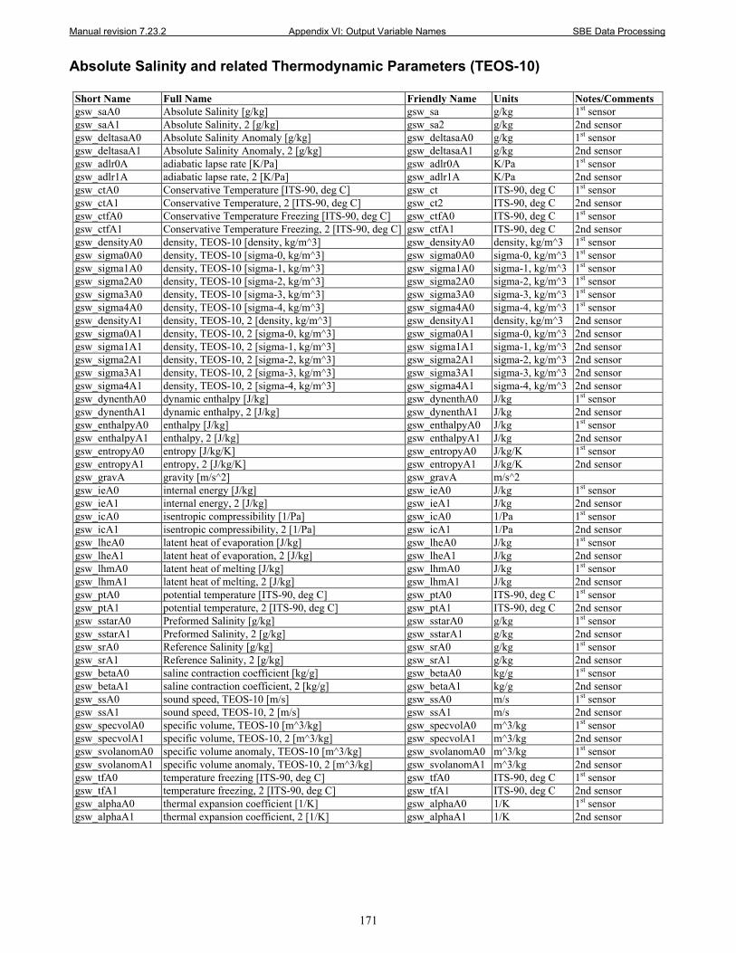
Manual revision 7.23.2 Appendix VI: Output Variable Names SBE Data Processing
171
Absolute Salinity and related Thermodynamic Parameters (TEOS-10)
Short Name Full Name Friendly Name Units Notes/Comments gsw_saA0 Absolute Salinity [g/kg] gsw_sa g/kg 1st sensor gsw_saA1 Absolute Salinity, 2 [g/kg] gsw_sa2 g/kg 2nd sensor gsw_deltasaA0 Absolute Salinity Anomaly [g/kg] gsw_deltasaA0 g/kg 1st sensor gsw_deltasaA1 Absolute Salinity Anomaly, 2 [g/kg] gsw_deltasaA1 g/kg 2nd sensor gsw_adlr0A adiabatic lapse rate [K/Pa] gsw_adlr0A K/Pa 1st sensor gsw_adlr1A adiabatic lapse rate, 2 [K/Pa] gsw_adlr1A K/Pa 2nd sensor gsw_ctA0 Conservative Temperature [ITS-90, deg C] gsw_ct ITS-90, deg C 1st sensor gsw_ctA1 Conservative Temperature, 2 [ITS-90, deg C] gsw_ct2 ITS-90, deg C 2nd sensor gsw_ctfA0 Conservative Temperature Freezing [ITS-90, deg C] gsw_ctfA0 ITS-90, deg C 1st sensor gsw_ctfA1 Conservative Temperature Freezing, 2 [ITS-90, deg C] gsw_ctfA1 ITS-90, deg C 2nd sensor gsw_densityA0 density, TEOS-10 [density, kg/m^3] gsw_densityA0 density, kg/m^3 1st sensor gsw_sigma0A0 density, TEOS-10 [sigma-0, kg/m^3] gsw_sigma0A0 sigma-0, kg/m^3 1st sensor gsw_sigma1A0 density, TEOS-10 [sigma-1, kg/m^3] gsw_sigma1A0 sigma-1, kg/m^3 1st sensor gsw_sigma2A0 density, TEOS-10 [sigma-2, kg/m^3] gsw_sigma2A0 sigma-2, kg/m^3 1st sensor gsw_sigma3A0 density, TEOS-10 [sigma-3, kg/m^3] gsw_sigma3A0 sigma-3, kg/m^3 1st sensor gsw_sigma4A0 density, TEOS-10 [sigma-4, kg/m^3] gsw_sigma4A0 sigma-4, kg/m^3 1st sensor gsw_densityA1 density, TEOS-10, 2 [density, kg/m^3] gsw_densityA1 density, kg/m^3 2nd sensor gsw_sigma0A1 density, TEOS-10, 2 [sigma-0, kg/m^3] gsw_sigma0A1 sigma-0, kg/m^3 2nd sensor gsw_sigma1A1 density, TEOS-10, 2 [sigma-1, kg/m^3] gsw_sigma1A1 sigma-1, kg/m^3 2nd sensor gsw_sigma2A1 density, TEOS-10, 2 [sigma-2, kg/m^3] gsw_sigma2A1 sigma-2, kg/m^3 2nd sensor gsw_sigma3A1 density, TEOS-10, 2 [sigma-3, kg/m^3] gsw_sigma3A1 sigma-3, kg/m^3 2nd sensor gsw_sigma4A1 density, TEOS-10, 2 [sigma-4, kg/m^3] gsw_sigma4A1 sigma-4, kg/m^3 2nd sensor gsw_dynenthA0 dynamic enthalpy [J/kg] gsw_dynenthA0 J/kg 1st sensor gsw_dynenthA1 dynamic enthalpy, 2 [J/kg] gsw_dynenthA1 J/kg 2nd sensor gsw_enthalpyA0 enthalpy [J/kg] gsw_enthalpyA0 J/kg 1st sensor gsw_enthalpyA1 enthalpy, 2 [J/kg] gsw_enthalpyA1 J/kg 2nd sensor gsw_entropyA0 entropy [J/kg/K] gsw_entropyA0 J/kg/K 1st sensor gsw_entropyA1 entropy, 2 [J/kg/K] gsw_entropyA1 J/kg/K 2nd sensor gsw_gravA gravity [m/s^2] gsw_gravA m/s^2 gsw_ieA0 internal energy [J/kg] gsw_ieA0 J/kg 1st sensor gsw_ieA1 internal energy, 2 [J/kg] gsw_ieA1 J/kg 2nd sensor gsw_icA0 isentropic compressibility [1/Pa] gsw_icA0 1/Pa 1st sensor gsw_icA1 isentropic compressibility, 2 [1/Pa] gsw_icA1 1/Pa 2nd sensor gsw_lheA0 latent heat of evaporation [J/kg] gsw_lheA0 J/kg 1st sensor gsw_lheA1 latent heat of evaporation, 2 [J/kg] gsw_lheA1 J/kg 2nd sensor gsw_lhmA0 latent heat of melting [J/kg] gsw_lhmA0 J/kg 1st sensor gsw_lhmA1 latent heat of melting, 2 [J/kg] gsw_lhmA1 J/kg 2nd sensor gsw_ptA0 potential temperature [ITS-90, deg C] gsw_ptA0 ITS-90, deg C 1st sensor gsw_ptA1 potential temperature, 2 [ITS-90, deg C] gsw_ptA1 ITS-90, deg C 2nd sensor gsw_sstarA0 Preformed Salinity [g/kg] gsw_sstarA0 g/kg 1st sensor gsw_sstarA1 Preformed Salinity, 2 [g/kg] gsw_sstarA1 g/kg 2nd sensor gsw_srA0 Reference Salinity [g/kg] gsw_srA0 g/kg 1st sensor gsw_srA1 Reference Salinity, 2 [g/kg] gsw_srA1 g/kg 2nd sensor gsw_betaA0 saline contraction coefficient [kg/g] gsw_betaA0 kg/g 1st sensor gsw_betaA1 saline contraction coefficient, 2 [kg/g] gsw_betaA1 kg/g 2nd sensor gsw_ssA0 sound speed, TEOS-10 [m/s] gsw_ssA0 m/s 1st sensor gsw_ssA1 sound speed, TEOS-10, 2 [m/s] gsw_ssA1 m/s 2nd sensor gsw_specvolA0 specific volume, TEOS-10 [m^3/kg] gsw_specvolA0 m^3/kg 1st sensor gsw_specvolA1 specific volume, TEOS-10, 2 [m^3/kg] gsw_specvolA1 m^3/kg 2nd sensor gsw_svolanomA0 specific volume anomaly, TEOS-10 [m^3/kg] gsw_svolanomA0 m^3/kg 1st sensor gsw_svolanomA1 specific volume anomaly, TEOS-10, 2 [m^3/kg] gsw_svolanomA1 m^3/kg 2nd sensor gsw_tfA0 temperature freezing [ITS-90, deg C] gsw_tfA0 ITS-90, deg C 1st sensor gsw_tfA1 temperature freezing, 2 [ITS-90, deg C] gsw_tfA1 ITS-90, deg C 2nd sensor gsw_alphaA0 thermal expansion coefficient [1/K] gsw_alphaA0 1/K 1st sensor gsw_alphaA1 thermal expansion coefficient, 2 [1/K] gsw_alphaA1 1/K 2nd sensor
Manual revision 7.23.2 Index SBE Data Processing
172
Index . .afm file · 15 .asc file · 15 .bl file · 15 .bmp file · 15 .bsr file · 15 .btl file · 15 .cnv file · 15 .con file · 15, 24, 141
reports · 146 SBE 16 · 28 SBE 16plus · 29 SBE 16plus V2 · 31 SBE 16plus-IM · 29 SBE 16plus-IM V2 · 31 SBE 19 · 33 SBE 19plus · 35 SBE 19plus V2 · 37 SBE 21 · 39 SBE 25 · 41 SBE 45 · 49 SBE 49 · 50 SBE 911plus · 26 SBE 917plus · 26
.dat file · 15
.hdr file · 15
.hex file · 15
.ini file · 15
.jpg file · 15
.mrk file · 15
.psa file · 15
.ros file · 15
.txt file · 15
.wmf file · 15
.xml file · 15
.xmlcon file · 15, 24, 141 reports · 146 SBE 16 · 28 SBE 16plus · 29 SBE 16plus V2 · 31 SBE 16plus-IM · 29 SBE 16plus-IM V2 · 31 SBE 19 · 33 SBE 19plus · 35 SBE 19plus V2 · 37 SBE 21 · 39 SBE 25 · 41 SBE 25plus · 43 SBE 37 · 47 SBE 45 · 49 SBE 49 · 50 SBE 911plus · 26 SBE 917plus · 26 SBE Glider Payload CTD · 51
A A/D count sensors · 56 Absolute Salinity · 96 Acceleration · 158 Algorithms · 148
Align CTD · 82 Altimeter · 57 ASCII In · 112 ASCII Out · 113 Average · 86 Average sound velocity · 153
B Batch file processing · 137 Bin Average · 86 Bottle Summary · 78 Bugs · 147 Buoyancy · 89
C Calculator
seawater · 132 Calibration coefficients · 52
A/D count sensors · 56 altimeter · 57 bottles closed · 55 conductivity · 54 exporting · 52 fluorometer · 57 frequency sensors · 53 GTD · 70 importing · 52 methane · 62 OBS/Nephelometer/Turbidity · 62 optode · 70 oxidation reduction potential · 63 oxygen · 55, 64 PAR/irradiance · 65 pH · 65 pressure · 55, 56, 57 pressure/FGP · 65 RS-232 sensors · 69 SBE 38 · 69 SBE 50 · 69 SBE 63 · 69 sound velocity · 55 suspended sediment · 66 temperature · 53, 56 transmissometer · 66 user polynomial · 68 voltage sensors · 57 WET Labs C-Star · 69 WET Labs ECO · 69 WET Labs WETStar · 69 Zaps · 68
Cell Thermal Mass · 91 Command line operation · 136 Command line options · 134 Compatibility issues · 147 Conductivity · 54
specific · 155 Configuration
calibration coefficients · 52 calibration coefficients – RS-232 sensors · 69 file · 15, 24, 141, 146
Manual revision 7.23.2 Index SBE Data Processing
173
Configure · 24
calibration coefficients – A/D count sensors · 56 calibration coefficients - frequency sensors · 53 calibration coefficients - voltage sensors · 57 Glider Payload CTD · 51 SBE 16 · 28 SBE 16plus · 29 SBE 16plus V2 · 31 SBE 16plus-IM · 29 SBE 16plus-IM V2 · 31 SBE 19 · 33 SBE 19plus · 35 SBE 19plus V2 · 37 SBE 21 · 39 SBE 25 · 41 SBE 25plus · 43 SBE 37 · 47 SBE 45 · 49 SBE 49 · 50 SBE 911plus · 26 SBE 917plus · 26
ConReport.exe · 146 Contour · 118 Corrected irradiance · 158 C-Star · 69
D Data Conversion · 72 Data processing · 18 Density · 149 Depth · 150
seafloor · 150 Derive · 93 Derive TEOS-10 · 96 Derived parameter formulas · 148 Descent rate · 158 Dynamic meters · 149
E ECO · 69 Editing data files · 18 EOS-80 · 93 Exporting calibration coefficients · 52
F FGP · 65 File extensions · 15 File formats · 15 Filter · 99 Fluorometer · 57 Formulas · 148 Frequency sensors · 53
G Geopotential anomaly · 149 Glider Payload CTD · 23, 51 GTD · 70
H Headings · 159
I Importing calibration coefficients · 52 Installation · 9 Instrument configuration · 141, 146 Irradiance · 65, 158
L Limited liability statement · 2 Loop Edit · 102
M Mark Scan · 80 Methane · 62 Modules · 8
dialog box · 11
N Nephelometer · 62 Nitrogen saturation · 157
O OBS · 62 Optode · 70 ORP · 63 Oxidation reduction potential · 63 Oxygen · 64, 156 Oxygen saturation · 157 Oxygen solubility · 157
P PAR · 65, 158 Parameter formulas · 148 Parameter names · 159 pH · 65 Plot · 118 Plume anomaly · 155 PostProcSuite.ini file · 15 Potential temperature · 154 Potential temperature anomaly · 154 Practical salinity · 93 Pressure · 55, 56, 57, 65 Processing data · 18 Processing sequence
Glider Payload CTD · 23 profiling CTDs · 20, 23 SBE 16 · 21 SBE 16plus · 21 SBE 16plus V2 · 21 SBE 16plus-IM · 21 SBE 16plus-IM V2 · 21 SBE 19 · 20 SBE 19plus · 20, 23 SBE 19plus V2 · 20 SBE 21 · 21 SBE 25 · 20 SBE 25plus · 20 SBE 37 · 22 SBE 39 · 23 SBE 39-IM · 23 SBE 39plus · 23
Manual revision 7.23.2 Index SBE Data Processing
174
SBE 45 · 21 SBE 48 · 23 SBE 49 · 20 SBE 911plus · 20
Profiling CTDs · 20, 23
R Reports
.con or .xmlcon file · 146 Rosette Summary · 78 RS-232 sensors · 69
S Salinity · 151 Saturation · 157 SBE 16 · 21, 28 SBE 16plus · 21, 29 SBE 16plus V2 · 21, 31 SBE 16plus-IM · 21, 29 SBE 16plus-IM V2 · 21, 31 SBE 19 · 20, 33 SBE 19plus · 20, 35 SBE 19plus V2 · 20, 37 SBE 21 · 21, 39 SBE 25 · 20, 41 SBE 25plus · 20, 43 SBE 37 · 22, 47 SBE 38 · 69 SBE 39 · 23 SBE 39-IM · 23 SBE 39plus · 23 SBE 45 · 21, 49 SBE 48 · 23 SBE 49 · 20, 50 SBE 50 · 69 SBE 63 · 69 SBE 911plus · 20, 26 SBE 917plus · 26 SBE Data Processing
Align CTD · 82 ASCII In · 112 ASCII Out · 113 Bin Average · 86 Bottle Summary · 78 Buoyancy · 89 Cell Thermal Mass · 91 Configure · See Configure creating water bottle files · 75 Data Conversion · 72 Derive · 93 Derive TEOS-10 · 96 File Setup tab · 13 Filter · 99 getting started · 10 Header View tab · 13 Loop Edit · 102 Mark Scan · 80 module dialog box · 11 modules · 8 problems · 147 Rosette Summary · 78 SeaCalc III · 132 Section · 114 Split · 115
Strip · 116 Translate · 117 use · 10 Wild Edit · 104 window · 10 Window Filter · 106
Sea Plot · 118 SeaCalc III · 132 Seafloor depth · 150 Seasoft
file extensions · 15 file formats · 15 programs · 6
Section · 114 Sigma-1 · 149 Sigma-2 · 149 Sigma-4 · 149 Sigma-t · 149 Sigma-theta · 149 Software
problems · 147 Solubility · 157 Sound velocity · 55, 152
average · 153 Specific conductivity · 155 Specific volume · 149 Specific volume anomaly · 149 Split · 115 Strip · 116 Summary · 6 Surface PAR · 158 Suspended sediment · 66
T Temperature · 53, 56
potential · 154 TEOS-10 · 132 Thermosteric anomaly · 149 Translate · 117 Transmissometer · 66 Troubleshooting · 147 TS plot · 118 Turbidity · 62
U Updates · 9 User polynomial · 68
V Variable names · 159 Velocity · 158 Voltage sensors · 57
W Water bottle files · 75 WETStar · 69 Wild Edit · 104 Window Filter · 106
Z Zaps · 68