SATISFYING URBAN LAWN WATER REQUIREMENTS

FROM ON-SITE RETENTION

by

JAMES CLINTON WALKER, B.S.C.E.

A THESIS

IN

CIVIL ENGINEERING

Submitted to the Graduate Faculty of Texas Tech University in Partial Fulfillment of the Requirements for

the Degree of

MASTER OF SCIENCE

IN

CIVIL ENGINEERING

Approved

August, 1986

/ • lO o. -- f ACXNOWLEDOvlENTS

I would like to give my sineara thanks to my eommittaa

chairman, Dr, B. J, Claborn, who sparked my interest in the

field of water rasoureas anginaaring and for all his help

toward tha eompletlon of this thesis. I would also like to

thank tha other members of my eommittaa. Dr. R, H. Ramsey

III and Dr. L. V. Urban, for thair help.

I am most grateful to my parents Jim and Louisa

Walker, Without thair hard work, support, and lova this

eould navar have baan aeeomp1ishad.

i i

TABLE OF CONTENTS

ACKNOWLEDGMENTS i i

LIST OF TABLES v

LIST OF FIGURES vi

I, INTRODUCTION 1

II. LITERATURE REVIEW 4

Irrigation Management Praetieas . . . . 4

Evapotranspirat ion 5

Percolation 11

Soil Moisture Storage 12

Praeipi tat ion 16

Irrigation 16

Irrigation Effieianey 17

Storage Devices 18

III. LAWN IRRIGATION AND STORAGE REQUIREMENTS

BY COMPUTER SIMULATION 19

Evapotranspiration 20

Effective Praeipitation 29

Soil Moisture Storage 29

Pereolation 31

Irrigation Required 32

Cistern Storage 33

1 i i

1 V

IV. RESULTS 35

V. CONCLUSIONS AND RECOMENDATIONS 46

Conelusions 46

Reeomandations 47

Other Conservation Considerations . . . 49

LIST OF REFERENCES 51

APPENDICES 55

A. COMPUTER 40DEL 56

B. DESIGN EXAMPLE 60

C. ECONOMIC ANALYSIS 6 3

LIST OF TABLES

1. Comparison of Tueson and Lubboek Water Use by

Turf Grass , 25

2, Results of Design Example 41

3. Eeonomie Comparison of Cistern Alternatives . , , 43

4, 1986 Water Rate Structure for Lubboek Texas . . , 44

LIST OF FIGURES

1. Available Water Profile 14

2. Percent Available Water Extracted 15

3. Soil Moisture Balance 21

4. Potential Evapotranspirat ion by Modified Penman . 24

5. Consumptive Use 26

6. Crop Growth Coefficient, K^ 27

7. Probability of Failure 37

8. Required Storage Volume as a Function of

Impervious Area and Risk 39

9. Retention Volume Design Curves 40

10, Retention Volume Design Example 62

vi

CHAPTER I

INTRODUCTION

Most water supplies of tha arid and semi-arid regions

of the United States have limited lifetimes. Many of these

areas rely almost solely on water from aquifer formations

that are being mined of their water because of minimal

amounts of natural recharge. Water is a major factor in

the soeio-eeonomi e growth of these areas and as these

eonmunities grow so does their demand for water. As a

result, the search for more water and for alternatives to

its use has begun in most arid and semi-arid regions.

In all areas of use, water conservation has taken on

new meaning. Agriculture and industry have made major

advancements in water conservation, naeessitatad by

ineraasing water costs. Increases in cost result from the

tremendous expense involved with the development of new

sources and the rising costs of treatment and distribution,

Inereased costs and resource scarcity eonsiderations

neeassitata attention to conservation praetiees in the

urban environment.

Devices such as flow rate and reduction attachments to

water fixtures in the home are available for residential

users to save water. However, these save small quantities

of water and are used only by a small percentage of the

homeowners.

Factors influencing the amount of residential water

use are climate, water availability, metering, residential

density, and the eeonomie status of the homeowners (Cottar

at al., 1974), Linawaavar, in his 1967 landmark paper,

reported an average use per dwelling per day of 433 gallons

in the western states. Lawn irrigation aeeounts for

approximately one-half of all urban water use annually

(Borrelli et al,, 1981), This suggests lawn Irrigation is

a primary candidate for urban water conservation

praetlees.

Lawn irrigation demands are seasonal in nature causing

peak flow requirements during sunrmer months. Peak rates

establish design criteria for the municipal water system.

By decreasing peak flow rates, cost savings can be

obtai ned.

Most preeipitation in urban areas appears as runoff

from the landscape and impervious areas. This runoff also

causes stormwater management problems.

On residential lots in arid and semi-arid regions

enough praeipi tation is available for maintenance of some

lawn area, but preeipitation often oceurs at the wrong time

of the year. Storage of excess preeipitation is an obvious

teehnieal solution to this problem. This study addresses

3

the teehnieal and eeonomie feasibility of on-site storage

of these waters.

The specific objectives of this research are to:

1) Determine irrigation requirements for urban

lawns sufficient to maintain the aesthetic

appeal of tha lawn,

2) Determine the amount of rainfall that ean be

captured and saved for irrigation purposes,

3) Determine the size of storage container

(cistern) required for residential lot, and

4) Determine the eeonomie feasibility with or

without monetary additional incentives.

Information necessary to meet the first objective is

available from the literature and is reviewed in Chapter

II. A daily simulation model has been written to

aeeomplish the second and third objectives. This model is

described in Chapter III. Results of the application of

this model to elimatie conditions for Lubboek, Texas are

discussed in Chapter IV. These results, together with the

water rate structure for Lubboek are used in the

feasibility analysis.

CHAPTER II

LITERATURE REVIEW

Preeipitation raaehing tha lawn will infiltrate into

the soil or runoff to become part of the stormwater

management problem. Water infiltrated becomes available for

use by the lawn, or percolates through the root zone and is

lost to the plants. This chapter reviews literature

pertinent to the management of lawn irrigation and to the

physical processes Involved in the use of water by the

I awn.

Irrigation Management Praetiees

The primary purpose of irrigation is to maintain tha

soil moisture in a range that permits plants to adsorb water

(Pair, 1975 ) . Deficit irrigation oeeurs when the plant is

given less available water than its maximum uptake rate.

Limiting the available water ean be detrimental and even

fatal to the plant. But, If carefully controlled, maximum

crop yields ean oeeur and at the same time use less water.

Decisions about irrigation management are often made without

considering the effects of deficit irrigation (Martin et

al., 1984). Kneebone et al. (1979) showed that application

of water above evaporative demands was wasteful and that

erops, specifically turf grass, can be grown with

considerably less water. Factors that interact to determine

water use by turf grass are; the grass itself (Biran et al.,

1981); the microclimate conditions (Jensen, 1980); the soil

(Kneebone et al., 1979); and the management praetiees

(Feldhake et al., 1984; Biran at al., 1981). These were

reported by Borrelli at al, (1981).

Evapotranspirat ion

ET is tha sum of water evaporated from the soil and the

amount of transpiration from the plant. Potential ET is the

ET rate when water is not a limiting factor. Numerous

studies on ET have been performed and there are many methods

available to estimate its magnitude. ET rates are difficult

to determine because of the many factors which influence ET.

The most important factors are leaf area, stage of crop

growth, climate, and tha soil (Pair, 1975), Most methods

contain valid features but no existing method is universally

adequate when modeling meteorological data (Borrelli et al,,

1985).

The fundamental equation to begin with in ET estimates

is tha Penman equation. Penman's original work In 1948

studied evaporation that occurred from open water, bare

soil, and grass. He reasoned that two requirements had to

be met in order for evaporation to oeeur. The first

6

requirement was the input of energy to provide for the

latent heat of vaporization. The second, which he termed

sink strength, accounted for tha disposition of the vapor.

Both the sink strength and energy balance are included in

his original equation which states;

E Q = (H A + 0.27 Ea) / ( A + 0.27) (1)

where, E Q = evaporation rate in mm/day,

H = net radiant energy available at the

surface, cal/cm2/day,

A = temperature dependent constant, and

EQ - expressed as the "drying power" of

air, including the vapor pressure

deficit and a function of wind speed

(Penman, 1948).

The Penman equation incorporates many parameters including

solar radiation, wind speed, and relative humidity which are

termed secondary weather parameters. While obtaining a high

degree of accuracy, + 10 percent of actual ET (Doorenbos et

al., 1977), a major disadvantage is that values of these

secondary weather parameters are often unavailable at the

location where ET estimates are needed.

A modification to the original Penman equation was

developed at the Texas A & M University Agricultural

Research Extension Center located near Lubboek, Texas.

Their Modified Penman equation is;

1 Q.27 ETp = 0,00673 A + 0.27 (Rn) + A+ 0.27 (15.36)

( 1 + 0.01 W) (e s - ed) (2)

ETp = potential evapotranspiration,

mm/day,

Rn = net solar radiation * Rfaetor»

ea1/cm^/day,

^factor = adjustment for solar radiation

based on the day of the year,

e's = (esmax " smin)/ 2, millibars,

®smax» ®smin ~ saturation vapor pressure

for maximum and minimum

temperatures, respectfully,

mi I I i bars,

e^ = [ esmax^"^^-^ • "' relative humidity)

+ ^smin (minimum relative

humidi ty)] / 2, mi I 1ibars,

W = average wind speed, miles/day,

and,

A = temperature dependent slope

cons tant

(Gregory, 1982).

ET rate prediction methods that use principally

temperature data are widely used and accepted. Soma of the

8

mora common forms using temperature are the original Blaney-

Criddle method, the Soil Conservation Service (SCS) (Soil

Conservation Service, 1970), and the United Nations Food and

Agriculture Organization (FAO) (Allen et al,, 1986)

modifications to the Blaney-Criddle formula.

The original Blaney-Criddle formula was developed to

compute consumptive use using mean air temperature, the

percentage of daytime hours, and relative humidity. The

equation was later modified by Blaney and Criddle erasing

the humidity term to compute consumptive use (Blaney et al,,

1965). Consumptive use is equal to potential ET which is

defined as the amount of water lost through ET when the

amount of available water is not a limiting factor. That

is, the plant always has an adequate supply of water. The

Blaney-Criddle formula may be written as;

U = F * K (3)

where, F = t • p / 100

t = mean air temperature in degrees

Fahrenhei t;

p = percent daylight hours; and

K = kt * kc

kt = climatic coefficient, 0.0173t - 0.314;

kc = crop growth coefficient

(Soil Conservation Service, 1970).

9

Assumptions include:

1) seasonal consumptive use (U) varies directly

with the consumptive use factor (F);

2) actively growing crops have adequate water

throughout the growing season;

3) soil fertility is uniform;

4) the yields of forage crops vary only with the

length of growing season (Blaney et al.,

1965).

The Blaney-Criddle method has been used worldwide, espe­

cially in the western United States (Gregory, 1982).

Because different areas can have the same consumptive use

factor and at the same time have different ET rates, the

estimates using Blaney-CriddIe are usually given a ± 25

percent margin of error (Doorenbos et al., 1977).

A study in Idaho by Allen et al. (1986) used the FAO

Blaney-Criddle formula. The difference between the original

and the FAO version is that "correction factors" are used to

adjust for local weather and climatic conditions. Allen et

al. (1986) calibrated and compared the results of the FAO

Blaney-Criddle formula to the Penman equation and to daily

lysimeter measurements of alfalfa ET, The FAO Blaney-

Crlddle formula was shown to give excellent estimates of ET,

when locally calibrated, compared to the field measurements

and to the Penman equation using secondary weather para­

meters.

10

Borrelli et al. (1981) studied turf grass consumptive

use in an urban environment. Field measurements with

lysimeters were used to calibrate the SCS version of the

Blaney-Criddle formula. Research areas were located in

Wyoming, Colorado, Arizona, and California. Several

varieties of turf grass were used. Both a high and low

management regime were used in the study. High management

plots were those receiving frequent mowing, irrigation, and

fertilizer application. The low management plots were cared

for in accordance with the estimated degree of care by the

average homeowner. Mantel 1 (1966) and Dernoeden et al,

(1978) found that management practices ean significantly

affect turf grass quality especially under drought eondl-

t ions.

In addition to determining the consumptive use of

turf grass in urban environments, Borrelli et al. (1981)

also developed values for the crop growth coefficient, k^,

for each grass tested. The crop growth coefficient, kc,

relates the crop ET, in this case turf grass, to a reference

crop ET, usually alfalfa. Crop growth coefficients vary

according to climate, crop characteristics, length of

growing season, and time of planting (Doorenbos et al.,

1977). Borrelli et al. (1981) also stated that kc has a

meteorological component which is not completely represen­

tative of the crop.

11

Research by Feldhake et al. (1983) studied changes in

ET rates with respect to urban environments and management

practices. They found that actual turf grass ET can vary

greatly from predictions based on the regional climate.

Trees, shrubs, fences, and buildings influence wind velocity

and direction which can cause significant variation in ET

rates making them very site specific (Davenport, 1965;

Danielson et al,, 1979).

Percolat i on

Percolation is defined as the amount of water that

passes completely through the root zone. Pereolation will

occur when the infiltrated water summed with the water

already In the soil exceeds field capacity. Field capacity

is technically defined as having 0.3 bars of soil water

suction or is more commonly described as the amount of soil

water remaining after free drainage has occurred. Free

drainage is usually considered complete after two days. In

the modeling studies by Steichen et al. (1984) and Martin et

al. (1984) both divided the soil into layers. Martin et al.

(1984) simulated soil moisture distribution using six

layers. The first layer was 2 inches thick, the second and

third were 4 and 6 inches respectfully, and the other layers

were 12 inches each. Excess water was made available for

crop use for one day and then was assumed to drain.

Steichen et al. (1984) separated the soil into two layers.

12

When field capacity was reached the excess water cascaded to

the next layer after two days.

The amount of percolation, which is assumed to be

permanently lost from the system, depends on the storage

volume of the soil and the depth of soil modeled. The rate

at which water moves down through the soil depends largely

on the structure of the soil and the type of soil, e.g.,

sand, loam, and clay. Soil structure is the grouping or

arrangement of soil particles and influences percolation

rates by changing the porosity of the soil. Porosity Is the

amount of void space between the soil particles. Sandy

soils percolate water faster than clayey soils because sandy

soil has larger particles and larger pore openings than

c lay.

Soil Moisture Storage

The water storage capacity of soil is dependent upon

many factors. Water is physically held in the soil by

gravitational, capillary, and hygroscopic forces. Gravi­

tational water Is that water In excess of field capacity

which drains. Capillary water is water held In the soil

and is available to plants. Hygroscopic water is a

molecular layer bound to the soil particles (Brady, 1984).

The available soil moisture for crop use, the capillary

water, ranges between field capacity, previously defined,

13

and the permanent wilting point (Pair, 1975). The permanent

wilting point is usually defined at 15 bars of soil water

suction, but more descriptively is the point at which the

plant can no longer extract moisture from the soil. Martin

et al. (1984) found that in the upper 20 inches of a silty

clay loam, corn eould extract moisture down to the permanent

wilting point, (see Figure 1.) They also determined that,

below about 20 inches, the moisture extracted by the corn

decreased linearly to field capacity.

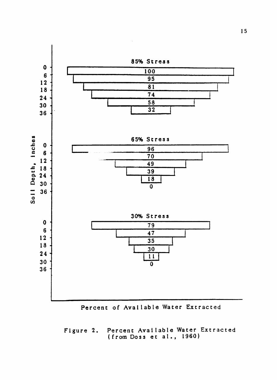
Research conducted by Doss et al. (1960) estimated the

amount of moisture removed by various types of turf grasses

at different depths based on root concentrations. Root

distribution was determined by 3-inch core samples, soil

profile samples, and soil moisture extraction patterns.

Their research included three soil moisture regimes. Soil

moisture stress was established at 30 percent, 65 percent,

and 85 percent of the total available moisture In the top 24

inches of soil. With each type of turf grass, including

common bermuda, the rooting depth decreased as soil moisture

increased, (see Figure 2.) Also, between species of turf

grass, the greatest variation of root depth was 6 inches and

this difference occurred in the soil moisture regime with

the greatest stress. They found the upper foot of soil to

be the most important with respect to soil moisture extrac­

tion because It contains approximately 76 percent of the

root s.

14

CO

4)

U C

0) o OS

u 3

O

cn

o

o. 4)

Q

0.10 0

10

20-

30-

« 40-1 CO

50-

60-»

Volumetric Moisture Content, decimal

0.15 0.20 0.25 0.30 0.35

Field Capacity

Plant Extractable Water Limit

-15 -1/4

Soil Moisture Potential, bars

Figure 1. Avallable Water Profile (from Martin et al., 1984)

15

0 6 12 Id 24 30 36

«0

Ji

u c

• JB ^4

a 4) a —

o en

0 6

12 18 24 30 36

0 6 12 Id

24

30 36

85% Stress

100 95 81 74 58 32

65% Stress

96 70 49 39 18

30% Stress

79 47 35

30 11

Percent of Available Water Extracted

Figure 2. Percent Available Water Extracted (from Doss et al., 1960)

16

Precipi tat ion

The amount of precipitation that does infiltrate into

the soil for plant use is termed effective precipitation.

The amount of effective precipitation is usually computed as

what remains after subtracting the amount of interception

storage and runoff from the total amount of precipitation

received. However, the amount of interception and runoff

can vary according to; 1) total precipitation, 2) intensity

of precipitation, 3) intake rate of soil, 4) water-holding

capacity of the soil, 5) ET rate of the crop, and 6) timing

of precipitation in relation to irrigation (Pair, 1975).

Both Steichen et al. (1984) and Martin et al. (1984) used

the SCS method to determine runoff in their models. How­

ever, only Steichen et al. (1984) accounted for interception

by initially subtracting 0.1 inches from the daily precipl-

tat ion.

I rr igat ion

"Irrigation is the quantity of water, exclusive of

precipitation, required to maintain the desired soil

moisture" (Pair, 1975). Aesthetic quality of the turf grass

is the primary objective of the Irrigation applied to the

lawn. Feldhake et al. (1984) studied the effects of

turf grass quality In Colorado when ET was reduced below the

maximum rate by deficit irrigation. Steichen et al. (1984)

said that ET declines linearly to zero at the permanent

17

wilting point when soil moisture falls below 0.3 of the

available water capacity. Feldhake et al. (1984) explained

that, when ET is reduced to 73 percent of maximum rate by

deficit irrigation, there was only a small decrease in lawn

quality. Lawn quality was evaluated as the percent live

blomass visible from the canopy. Their results support the

fact that the major effect of 27 percent deficit irrigation

Is a decrease In plant growth and that the aesthetic

characteristics decrease because increased stress causes

further damage to the plant. Feldhake et al. (1984) also

noted that the 27 percent decrease In observed Colorado may

be different for other climatic conditions.

Irrigation Efficiency

Irrigation efficiency is the ratio of the amount of water

that reaches the root zone for crop use to the quantity

applied. Most homeowners use sprinkler Irrigation to water

their lawns. Water lost in sprinkler Irrigation results

from evaporation of the spray, evaporation from the soil

surface, interception storage, sprinkler overlap, runoff,

and percolation (Pair, 1975). Sprinkler efficiencies can

change from day to day. Work at the Redfield, South Dakota

Experiment Station (1954) found that sprinkler Irrigation

efficiencies can range from 65 to 95 percent. Frost et al.

(1956) determined that for all weather conditions, doubling

the wind velocity approximately doubles the Irrigation

18

losses. They also determined that most of the losses are

directly related to the vapor pressure deficit. Another

study performed at Lubbock by Gerst et al. (1982a) found

that greater evaporation losses occurred from sprinklers

with lower flow rates, suggesting that the type of sprinkler

used can also effect the irrigation efficiency.

Storage Devices

Literature as it pertains to permanent storage in this

context Is virtually nonexistent. Blendermann (1979)

suggested the use of a dry well to act as a detention

container for roof runoff. The stormwater then leached Into

the soil. The main objective of his study was to dispose of

the water and not to retain it for some use. Other material

found discussed the capture of precipitation with the

intention of improving stormwater management, not for

conservation purposes.

CHAPTER I I I

LAWN IRRIGATION AND STORAGE REQUIREMENTS

BY COMPUTER SIMULATION

The purpose of this chapter is to explain the

methodology used to develop the computer model. Each aspect

of the model is separated by subheadings. The computer

model will determine the amount of Irrigation required to

maintain a green lawn and to determine the storage volume

required for the cistern.

A continuous hydrologlc simulation model of crop water

requirements was developed by Steichen et al, (1984) to

evaluate the risk of insufficient water for supplemental

irrigation. They suggested that to access the reliability

of a system designed to reduce risk, an observation of

system interactions must comprise at least 25 years of data

including one or two significant droughts. Their procedure,

a mass balance, or in this case a soil water balance, was

considered a valid approach from an engineering standpoint

to solve a problem of this type. Another computer model by

Martin et al. (1984) was developed to simulate the effects

of deficit irrigation on a crop. They also used a dally

19

20

soil moisture balance to estimate moisture stress as it

affected crop yields.

The soil moisture balance, shown in Figure 3, includes

water entering or leaving the system. The sum of water

input minus the water output Is equal to the change In

storage of the system with respect to time. This is shown

in Equation 4, which forms the basis of the computer

s imuI at i on.

Z Input - I Output = A Storage / A Time (4)

The storage system is the soil profile. The time step was

chosen to be one day because most hydrologlc data is

available on a daily basis. Bermuda grass is used in this

study because it is the most prevalent turf grass in the

desert southwest (Kneebone et al., 1979). The soil moisture

balance is used as the overall modeling technique, (see

Figure 3.)

Evapotranspiration

ET is moisture lost through evaporation from the soil

and the moisture transpired through the leaves of plants.

As shown in Chapter II, many accepted methods are available

to estimate water loss through ET. Most of these methods

have been developed to estimate agricultural crops, rather

than for turf grasses in an urban environment as is needed

21

EFTECTIVE PRECIPITATION EVAPOTRANSPIRATION IRRIGATION

^ 4 /

AVAILABLE STORAGE

PERCOLATION

Figure 3, Soil Moisture Balance

22

in this study. The study by Borrelli et al. (1981) was done

in several climatic regions in the United States on various

types of turf grasses in urban environments. Different lawn

management schemes were used and consumptive use was

determined by field measurement. The study site used by

Borrelli et al. (1981) that most closely represents the

climate of Lubbock, Texas is Tucson, Arizona. The Blaney-

Criddle crop growth coefficient, kc, for several varieties

of turf grass was determined from measured consumptive use

in Tucson. The values used in this study are from the

Tucson study for common bermuda grass under the low

management regime to represent average homeowner lawn care.

In order to use the consumptive use values found in the

Tueson study, a method was required to adjust for the

difference in climate between Lubbock and Tueson. Although

a wide range of methods are available, a choice of the

method was based on; 1) range of valid application; 2)

c1imatologicaIly similar to Lubbock, Texas; and, 3)

availability of the data required. On this basis, the Texas

A & M Modified Penman Method was chosen to relate the two

sites. (Gregory, 1984).

The Modified Penman method was chosen because it was

developed in the Lubbock area and incorporates solar

radiation, maximum and minimum temperature, maximum and

minimum relative humidity, and wind into the ET estimate.

Average monthly climatic data was gathered for both Tucson

23

and Lubbock over the ten year period 1971-1980, Solar

radiation values, determined from a table In Jensen et al.

(1973), are based on the latitude at each site. The average

monthly potential ET's for Tucson and for Lubboek were

determined by utilization of the Modified Penman equation.

Equation 2. The monthly potential ET's for Tucson and for

Lubboek are shown graphically in Figure 4.

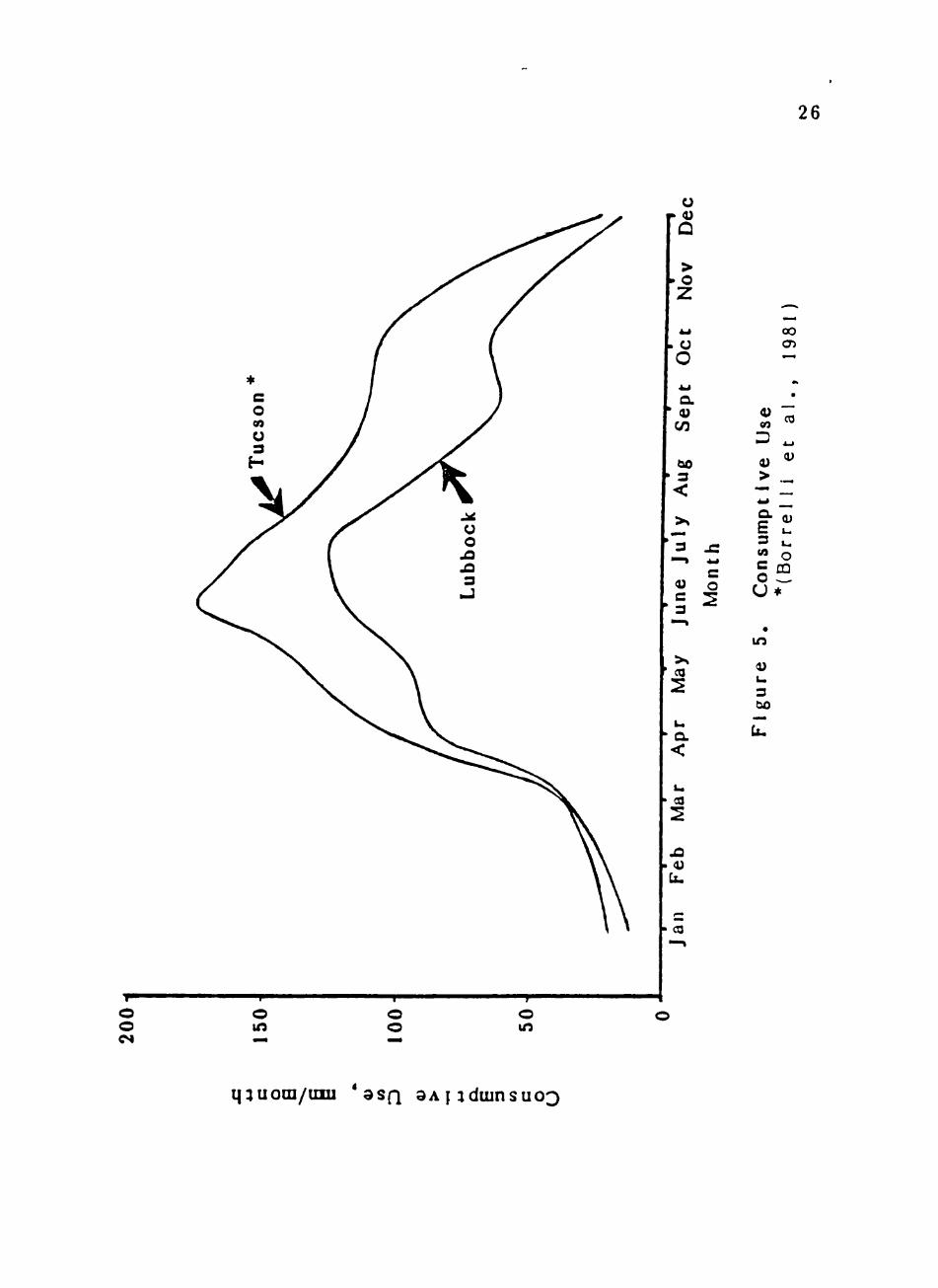
The monthly consumptive use for Lubboek was determined

by comparison of the ET found by the Modified Penman

equation for both Lubboek and Tucson. Equation 5 was used

to compute consumptive use for Lubboek.

CULubboek = ^^Tueson (^TLubbock / ETjucson) ^5)

CU = consumptive use

ET = potential evapotranspiration

The values for each term in Equation 5 are shown in Table 1

and Figure 5.

Using the consumptive use values for Lubbock, found by

Equation 5, the monthly crop growth coefficient in the

Blaney-Criddle method was determined. A similar deter­

mination was made using the low management data from the

Tucson study. Both sets of values are plotted In Figure 6.

Both curves differ significantly from the usual smooth shape

of crop growth coefficient plots (Soil Conservation Service,

1970). However, in a personal communication with Garrett

24

r- —p-o Oi -r-

00

- 1 — - T -

u 0) Q > o Z

. o O

Q.

00 3

<

C 4) O

E 2

2

o. <

CO

c 00

c O

CO

c CO c k4 CO

*- e o c o. a; CO CL >

CO ^ ^

c o

o > Q- J3

0)

3

Xep/uiu *uoi 58J idsuBJiodBAg l e p u s i o j

25

TABLE 1

Comparison of Tucson and Lubbock Water Use by Turf Grass

(mm/month)

MONTH

Jan

Feb

Mar

Apr

May

June

July

Aug

Sept

Oct

Nov

Dec

^^Tucs

127

155

204

267

322

363

278

249

251

223

171

143

ETLubbock^ CUxueson*^ CULubbock"*

95 20 15

20

37

88

96

247 178 121

122

204

224

230

26

37

105

134

227

182

142

143

102

151

124

111

110

81

123

91

63

71

49

105 26 19

^ Determined by Modified Pemnan, Equation 2, using climate data for Tueson, Arizona, 1971-1980.

2 Determined by Modified Penman, Equation 2, using climate data for Lubbock, Texas, 1971-1980.

3 Field measurements by Borrelli et al. (1981),

^ Consumptive use for Lubboek, Texas determined by Equa t i on 5.

26

O

o o o o

—r-o in

o r <u

Q

> L o Z

4 i 4

. U O .hi

a. ' 0) CO

tjo 3

<

>% . 3

" ^

0) c 3

" ^

CO

2

u a. <

u OJ

2 ^ <U

ix.

^

c o

—

(XD cn -^

M

.

3 ^ 4) ^ > .„

.farf

fj

Co

ns

u

*(B

or

• i n

V L. 3 (30

iZ

• CO

q^uom/um ' S S Q aAnduinsuoQ

27

o

—r-CO

—r-

u F (U

Q

> • o Z

A j

o o ^ 4

Q. ' <U CO

eio 3

<

>» — 3

"~* V c a "^

> N

n "2.

1 .

ex <

u fl

^

^ <u

U-

c CO

^ 4 ^

c o IE

" 4-1

c 0)

—" o — V M

V M

<u o

U r^

-» > o u

o Q. O L .

u •

CO

L.

3 bO

U,

"-* CO C75

"^ • k

. — CO

i J

a> . - M

— "^ <D u L .

o CQ • — •

if

in

o o

> M u 3 i 0 | j j 3 0 3 qiAvoJo dojo

28

Gill, Assistant Professor in Park Administration and

Landscape Architecture at Texas Tech University (1986), he

felt that these erratic values were the result of the lawn

management techniques used in the field study. Feldhake et

al. (1984) also found that under drought conditions,

management practices have a significant effect on turf grass

quality. Due to the erratic nature of the plot, weekly

values were determined graphically from the monthly values

in Figure 5, for use in the model.

Dally consumptive use estimates for Lubboek were

obtained using the Blaney-Criddle method. Meteorological

data was obtained from the Lubbock International Airport

weather station, which contained the longest and most

complete set of daily precipitation and maximum and minimum

temperature measurements in the area. Seventy years of

dally data were used covering the period 1914-1983. The

percent daylight hours is a function of the latitude of the

site being evaluated. Monthly values of percent daylight

hours, obtained from a table (Soil Conservation Service,

1970), were converted to weekly values to increase the

model's accuracy. Weekly crop growth coefficients were

determined as explained earlier. Weekly values of both

percent daylight hours and the crop growth coefficient, k^,

were required on a daily basis because a daily simulation

was used. The change was made by assigning Julian days to

represent the weekly values of the percent daytime hours and

29

kc values throughout the year. These changes enabled the

model to determine daily ET estimates.

Effective Precipitation

The methods used in similar studies to determine the

amount of effective precipitation are as varied as those for

ET estimates. As shown in Chapter II, some studies have

used the SCS method to compute the amount of runoff together

with an estimate of the interception storage. (Steichen et

al., 1984; Martin et al., 1984). Lubboek receives two types

of rainfall, thunderstorms and low intensity frontal storms,

and each occur at fairly predictable times of the year.

Because of this, assumed effective precipitation factors are

used for each type of storm depending on the day of the

year. Between May 15 and October 15 the effective

precipitation was assumed to be 40 percent of the total

preeipitation due to the high intensity thunderstorm

activity encountered during this part of the year. The

remainder of the year was assumed to experience 80 percent

effectiveness of the total precipitation due to low inten­

sity showers and snow melt.

Soil Moisture Storage

The amount of available water stored for plant use is

dependent on the type of soil. Water is available for use

30

by plants between the field capacity moisture content and

the moisture content at permanent wilting point. This

difference is known as the available water capacity of a

given sol 1.

Soil types are heterogeneous and vary from point to

point even within the same lawn. An Amari1lo-Urban land

complex was chosen for use in this study because it is

representative of the urban soils in the Lubbock area (Soil

Conservation Service, 1979). The Amari1 Io-Urban land

complex soil is approximately 55 percent Amarlllo soil, 35

percent urban land, and 10 percent other soils. The

permeability of this soil is between 2 to 6 Inches per hour

for the top 14 inches and 0.6 to 2 inches per hour below 14

inches. The available water capacity for the top 14 inches

ranges between 0.11 to 0.15 inches per inch and below 14

inches from 0.14 to 0.18 inches per inch (Soil Conservation

Service, 1979).

Feldhake et al. (1984) showed that turf grasses, when

moisture stressed up to 27 percent of the ET rate, suffered

little loss in aesthetic appeal. Moisture Is extracted at

various depths depending on the amount of stress placed on

the plant (Doss et al,, 1960), To determine the depth of

soil to be used in the model, the depth at which soil water

was extracted by bermuda grass roots was needed. Doss et

al. (1960) found that common bermuda grass placed under a

31

moisture stress of 30 percent of the available capacity

extracted only 11 percent of its total moisture below 24

inches of soil. Their study was done using a fairly uniform

soil throughout the tested depth, whereas the soils in

Lubboek have two distinct horizons with different available

water capacities in each. Available capacity is greater in

the lower horizon than in the upper layer. Because of this,

24 inches of soil was considered to be the active zone of

moisture availability and appropriate for the model.

The median values in the range of available water

capacity for both soil horizons was used. Summing the top

14 inches and then that in the 14 to 24 inches depth layer,

the available water capacity of the modeled soil profile was

found to be 3.43 inches.

PercoI at ion

Pereolation for the model was defined as the amount of

water that passed through the top 24 inches of soil.

Pereolation will occur when the Infiltrated water summed

with the amount of moisture already In the soil exceeds the

field capacity. After field capacity is reached in the

profile the amount of percolation will equal the amount of

Infiltrated water. The assumption was made that, as excess

water enters the soil, a like amount drains at the same rate

from the bottom of the 24 inch storage zone. While not

32

strictly correct, this assumption is adequate for the

mode 1.

I rr igat ion Requi red

The amount of irrigation required is the remaining

unknown variable in the soil moisture balance. Maintenance

of green color in the turf is the objective of the lawn

irrigation. Irrigation will be required during the growing

season to maintain good turf quality when the soil moisture

falls below 70 percent of the available water capacity as

shown by Felhake et al. (1984). Turf growth In Lubbock

generally begins about April 15th (Mertes et al., 1984).

Therefore, between April 1st and October 1st the percent

stress placed on the turf is 30 percent of the available

water capacity. During the rest of the year, the turf is

usually brown in color and irrigation would not make a

difference. For this reason, in the winter months the

percent stress was increased to 50 percent of the available

water capacity.

The amount of effective irrigation received is the

amount required to increase the soil moisture to field

capacity. Assuming most homeowners use sprinkler Irriga­

tion, an irrigation efficiency of 85 percent was used to

determine the total amount of water applied. This 85

percent sprinkler efficiency is an assumed value which can

33

range from 95 to 65 percent (Refield, South Dakota Expt.

Sta., 1954).

Cistern Storage

The simulation also includes a daily cheek on the amount

of water put into or removed from a cistern located on the

residential lot. Input to the cistern is obtained from

captured precipitation and the output is the amount of

irrigation required. To account for different sizes in

collection and application areas for each lot, the

noneontribut1ng and nonconsumptive areas, such as sidewalks

and patios, were subtracted from the total area. The ratio

of the amount of Impervious contributing area to the total

remaining area was termed the percent impervious area.

Equation 6 was used to compute the volume of storage In

Inches remaining at the end of each daily time step.

StOEnd = (%Imp)Prec(I) - ( 1-%Imp)Irr(I) + Stoint (6)

Stoint = cistern storage beginning of time step

StOEnd = cistern storage end of time step

Prec(I) = precipitation that day

Irr(I) = irrigation that day

%Imp = percent impervious

All variables, except percent Impervious area, are in units

of inches per unit area, which ean be converted to volume by

34

multiplying by the area covered. The initial cistern volume

was assumed empty at the beginning of the 70 year period of

record.

The completed model, shown in Appendix A, was run using

infinite and finite storage capacities. Finite storage

produced spills of excess water, while Infinite storage

volume prevented such losses. This was done to determine,

when using a certain size cistern, the protection achieved

from dependence on municipally supplied water for irriga­

tion.

CHAPTER IV

RESULTS

The model described in Chapter III was used to evaluate

the lawn irrigation requirements for Lubboek, Texas for the

period 1914-1983. The results of this analysis are

discussed in this chapter.

Input variables to the computer model are the percent

impervious area, as used in Equation 6, and the amount of

available cistern storage. The amount of impervious area

ranged from 10 percent to 90 percent in increments of 10

percent. For each of the nine values of percent impervious

area, available cistern storage was set at one, two, and

five inches and at infinite storage. All values In the

model, except percent impervious area, possess the units of

depth in inches, which can be converted to volume by

multiplying by the amount of total effective area.

Output generated from the computer model include

Irrigation required, water level in the cistern, amount of

overflow or spill from the cistern, and the amount of

treated water supplied from the city to meet irrigation

requi rement s.

35

36

Analysis of the output began by assembling the

generated values to represent the amounts of each variable

summed over the entire year of daily input. In this way,

for each set of values of percent impervious area and

available storage the amounts of spill and treated water

supplied were compiled. Over the seventy year period of

record, precipitation averaged 18.9 inches per year, and the

amount of irrigation required averaged 24.3 inches per year.

The maximum and minimum irrigation requirements were 30.1

and 14.9 inches, respectfully. A general "rule of thumb"

for irrigation in the Lubbock area is one inch per week

during the growing season which is approximately 24 weeks

long.

For each value of percent impervious area a computer

run of every tested available storage value was done. For

each set of input data, the number of years in which

irrigation is supplied from the city was determined.

Dividing the number of years when city water was required by

the total number of years examined, provided the percent

failure of the system.

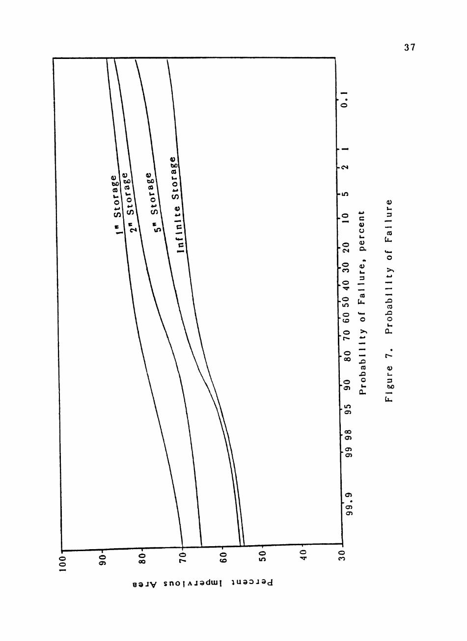
A probability graph was then developed for each set of

Input variables. Plots were completed for each value of

available cistern storage using the percent impervious area

versus the percent failure, (see Figure 7.)

The retention volume design curve was developed by

plotting the amount of storage in inches per unit area

37

o o o

c

- i n

. o

o CM

o eo u

3 O —

4_t

c 0)

u Urn

a. • k

0) L ^

0) L. 3

, CO

tl-

VhM

o >%

in

o CO

o o

o _ CO

o o

in 05

OO

CJJ

o O O

o in

I

o

CO

o

3 u bO 0. —

o CO

o a J V s n o | A j a d u j i l u a o j ^ d

38

versus the percent Impervious area from the probability

plots, (see Figure 8.) Isobars of the percent probability

of failure range from 50 percent to no failure. For

example, points for the 5 percent design curve were found by

reading the required impervious area from the ordinate

corresponding to the 5 percent probability for each storage

depth, (see Figure 7.)

For greater ease in determining cistern volumes the

storage scale was converted to gallons per square foot of

total effective area, (see Figure 9.) Total effective area

is the area of the lot remaining after subtracting the areas

that neither contribute to the cistern storage or present a

demand for irrigation. Such areas Include sidewalks and

patios, etc. Also, as previously defined, the percent

impervious area is the area of the lot that contributes

water to the cistern divided by the total effective area.

An example to determine cistern volume Is shown in Appendix

B. The results of the example are shown in Table 2 for

different probabilities of failure.

The cost of the cistern is determined by its size. As

shown in Appendix B, as the amount of protection from having

to irrigate with city water increases so does the volume and

cost of the cistern.

Several alternate types of cisterns are available and

have had an eeonomie analysis performed, (see Appendix C.)

One such alternative Is to build a basement under the house

39

15n

CO

u CO

^ 10-

c 3

E 3

5-

0-J ^ >-50 60 70 80

Percent Impervious Area 90 100

Figure 8. Required Storage Volume as a Function of Impervious Area and Risk

40

1 . 5 T

ca

>

o 0)

0)

CO

o

1.0-

CO ^^ •9 C

o

00 bO

e 3 o

> o bO CO u O

CO

0.5-

^ V 50 60 70 80 Total Eff-ectlve Area, percent

90 100

Figure 9. Retention Volume Design Curves

41

TABLE 2

Results of Design Example

Possible Storage Volume Required ^ai '"re (gallons)

5% 10,864

10% 8,848

20% 7,616

50% 5,264

42

with a wall partitioning the space into cistern and living

space. This arrangement Is not directly compared to other

alternatives on the basis of economics. However, a basement

is offered here as an alternative because a homeowner that

wants a basement might also consider installation of a

ci s tern.

Two alternatives that are compared economically are a

formed-in-pI ace concrete box and a fiberglass container.

Details of this comparison are shown In Appendix C and

sunmarized in Table 3. At the time of this writing, the

cost of a fiberglass tank is less than one formed of

concrete.

The remaining economic analysis depends on the savings

to the homeowner with respect to his water bill. The

current water rate structure of Lubboek is shown in Table 4.

Based on this declining rate system and Linaweaver's (1967)

annual average sprinkler use per dwelling unit per day of

186 gallons (Linaweaver, 1967), the average homeowner only

spends approximately $130 each year for lawn Irrigation in

Lubbock. By saving the homeowner only a portion of this

cost each year with this system, the economic shortcomings

of installing a cistern, whose initial costs range from

$5,000 to $8,000, is self-evident.

The results show that while a cistern used to capture

preeipitation for irrigation to maintain aesthetic

appearances is technically feasible, the economic

43

TABLE 3

Economic Comparison of Cistern Alternatives

Size of Ci stern Cistern 6,000 8,000 10,000

Alternative gal Ions gal Ions gal Ions

Formed-1n-place Concrete $8,325 $10,426 $12,246

Fiberglass Tank $5,013 $6,390 $7,337

44

TABLE 4

1986 Water Rate Structure for Lubbock Texas*

First 1,000 gallons $5.46 (minimum)

Next 49,000 gallons $1.13 /lOOO gal.

Next 200,000 gallons $ .97 /lOOO gal.

Over 250,000 gallons $ .91 /lOOO gal.

*Lubbock Power and Light

45

difficulties render this system's application extremely

IImi ted.

CHAPTER V

CONCLUSIONS AND RECONMENDATI ONS

The purpose of this chapter is to review the initial

objectives set forth in chapter I and to discuss each

objective as it pertains to the results of this research.

The final segment of this chapter is devoted to

recommendations to improve the application of this research

and to assist in the solution to the problem that brought

about this research: water use efficiency and conservation

in the arid and semi-arid urban environment.

Conelus i ons

The first objective of this research was to determine

the irrigation requirement for urban lawns that will

maintain a healthy green color. Using the soil moisture

balance simulation model the Irrigation required for

Lubbock, Texas was determined to average 24 inches per year.

This value agrees with common irrigation values for the

area.

The second objective established was to determine the

amount of rainfall available for capture and storage in the

cistern. Rainfall varies from year to year; the simulation

46

47

indicated adequate rainfall is available if large storage

volumes and large percent impervious areas are present.

This is shown in Figure 8.

Determining the size and type of cistern was the third

objective. The size of cistern is based on the probability

of failure determined by the previous two objectives.

Storage requirements depend on acceptable levels of risk,

and are shown in Figure 8.

The economic analysis indicated the savings in annual

expenditures for water in Lubbock, Texas are inadequate to

entice a homeowner to install a cistern at present water

cos t s.

Several types of cisterns are available for possible

use. Currently, fiberglass containers offer greater cost

savings as well as giving residential builders an easier

alternative to complicated structural work. Perhaps in the

future new technology can be applied to this problem.

Cost of accessories required for the cistern including

piping from gutters to cistern, a pump and power source, and

piping from the pump to irrigation equipment were not

included in the economic analysis.

Recoirmendat ions

Although the system is not presently financially

attractive, this research does have future application as

economic changes occur. The computer model can be modified

48

for other areas by using precipitation and temperature data

of the area and by adjusting the coefficients to values

representative of the site. The retention volume design

curves generated through this research can also be easily

used by the homeowner to determine the amount of money spent

for the cistern compared to the need of having to use

municipal water to irrigate.

Consideration of benefits accruing to the municipality

were beyond the scope of this study. Inclusion of these

benefits should be the topic of a follow up study to

determine the degree of participation warranted on the part

of the city.

Water harvesting in this study was limited to

impervious area. Additional harvesting from the lawn areas

is possible by shaping the area to drain to the cistern. A

study including this source should prove useful.

Quality of water In the cistern was beyond the scope of

this study. In many locations the quality of this water

will exceed that available from the city. Quality

deterioration in the cistern may also occur. The economic

impact of water quality in this plan should be studied.

An area of future research is to study a cistern system

for apartments and commercial buildings. Apartments and

commercial buildings usually have large amounts of

Impervious area compared to the amount of area that requires

49

irrigation. Also, the aesthetic appearance of these areas

is very important.

Other Conservation Considerations

A method of conservation is to Increase the efficiency

of Irrigation. Gerst et al, (1982b) found that irrigating

with heavy applications infrequently not only decreased the

losses through evaporation, but also increased the storage

of rainfall In the soil. Different forms of irrigation are

also available which can increase efficiency. Knowing when

to irrigate might be the best tool of all to Increase

efficiency. Installing tens Iometers, moisture blocks, or

other methods to determine soil moisture can aid the

homeowner in knowing when the lawn requires irrigation.

An increase in the cost of municipal water Is a must if

this system is to be used. Linaweaver et al. (1967) showed

that the cost of water to the homeowner had a definite

influence on the amount of water used and how it was used.

A substantial increase in Lubbock water rates will be

required to make this system attractive to the homeowner.

A city may wish to offer monetary incentives in the

form of reduced rates or tax adjustment to recognize savings

in capital costs occurring due to cistern use. These

savings occur because the city will not need to expand its

supply, treatment, and distribution systems as soon if new

residential areas are equipped with cisterns. This Is true

50

when the cistern uses some city water, if this use is

restricted by the installation of an orifice in the city

supply line to reduce peak demands.

The costs of water will certainly increase as supplies

diminish and treatment and distribution costs rise. As the

cost of water increases, each consumer will look at

different ways to conserve water. For this reason, research

of this type must be offered as an alternative to help

extend the life of our most precious resource.

LIST OF REFERENCES

Al len, Richard G. , and Wi I 1 lam O. Prui tt. "Rational Use of the FAO Blaney-Criddle Formula." Journal of Irrigation and Drainage Engineering ASCE Vol. 112 No. 2 May 1986: 139-155.

Biran, I. et al. "Water Consumption and Growth Rate of 11 Turfgrasses as Affected by ^Mowing Height, Irrigation Frequency, and Soil Moisture." Agronomy Journal Vol. 73 January-February 1981: 85-89.

Blaney, H. F., and Hansen E. G. "Consumptive Use and Water Requirements in New Mexico." Technical Report, New Mexico State Engineer 1965: 23-27.

Blendermann, Louis. Controlled Storm Water Drainage New York: Industrial Press Inc., 1979.

Borrelli, John, Marvin J. Dvoraeek, and Eugene P. Foerster. "Water Use by Turfgrasses: A Study of Deficit Irrigation and Esthetics." A Proposal to Investigate Dept. of Ag. Eng. Texas Tech Univ. 1985.

Borrelli, John et al. "Blaney-CrIddle Coefficients for Western Turf Grasses." Journal of Irrigation and Drainage Engineering ASCE Vol. 107 No. IR4 December 1981: 333-341.

Brady, NyIe C. The Nature and Properties of Soils 9th ed. New York: Maemillan, 1984.

Danielson, R. E., W. E. Hart, C. M, Feldhake, and P. M. Haw. "Water Requirements for Urban Lawns." Complet ion Report to OWRT Project B-035-WYO. 1979,

Davenport, D. C, "Versatility of a Small Grass Transpiro-meter," University of Nottingham School of Agriculture Report. 1965.

Dernoeden, P. H. and J, D, Butler, "Drought Resistance of Kentucky Bluegrass Cultlvars," Horticulture Science Vol, 13 June 1978: 667-668,

51

52

Doorenbos, J, and W. O, Pruitt, "Guidelines for Predicting Crop Water Requirements." Food and Agriculture Organization of the United Nations Vol. 24 1977: 30-TsT

Doss, Basil D., D. A. Ashley, and O. L. Bennett. "Effect of Soil Moisture Regime on Root Distribution of Warm Season Forage Species." Agronomy Journal Vol. 52 1960: 569-572.

Feldhake, C. M., R. E. Danielson, and J. D. Butler. "Turfgrass Evapotranspiration. I. Factors Influencing Rate in Urban Environments." Agronomy Journal Vol. 75 September-October 1983: 824-830.

Feldhake, C. M., R. E. Danielson, and J. D. Butler. "Turfgrass Evapotranspiration. II. Responses to Deficit Irrigation." Agronomy Journal Vol. 76 January-February 1984: 85-89.

Frost, K. R. and H. C. Schwalen. "Sprinkler Evaporation Losses." Agricultural Engineering Vol. 36 1956: 526-528.

Gerst, M. D., R. L. Postma, and C. W. Wendt. "Distribution and Application Losses from Home Lawn Sprinklers Under Field Conditions." Urban Water Conservation Research at Lubbock, 1981. The Texas Agricultural Experiment Station Technical Report No. 82-2, 1982a.

Gerst, M. D., R. L. Postma, and C. W. Wendt. "Comparison of Three Different Irrigation Regimes on Water Use Efficiency in Turf." Urban Water Conservation Research at Lubbock, 1981. The Texas Agricultural Experiment Station Technical Report No. 82-2, 1982b.

Gill, Garrett. Assistant Professor of Landscape Architecture, Texas Tech University. Personal Communication. 1986.

Gregory, David R. "The Influence of Evapotranspiration Rates and Cropping Sequences in Sizing Large Scale Land Application Systems," M, S, Thesis, Texas Tech University 1982,

Jensen, Marvin E,, ed. Consumptive Use of Water and Irrigation Water Requirements New York: American Society of Civil Engineers 1973: 22-23,

53

Kneebone, William R. and Ian L. Pepper, "Water Requirements for Urban Lawns." Project Completion Report to Office of Water Research and Technology Project B-035-WYO Wyoming Water Resources Research Institute. September 1979.

Kneebone, William R. and Ian L. Pepper. "Consumptive Use by Sub-irrigated Turfgrass under Desert Conditions." Agronomy Journal Vol. 74 May-June 1982: 419-423.

Linaweaver, F. P., John C. Geyer, and Jerome B. Wolff. "A Study of Residential Water Use." Federal Housing Administration Technical Studies Program U.S. Government Printing Office, Washington D.C. 1967.

Mahoney, William D. , ed. Building Construction Cost Data, Kingston, Ma,: R. S. Means Company, Inc. 1985.

Mantell, A. "Effect of Irrigation Fequency and Nitrogen Fertilization on Growth and Water Use of a Kikuyugrass Lawn." Agronomy Journal Vol. 58 1966: 559-561.

Martin, Derrel L., Darrell G. Watts, and James R. Gllley. "Model and Production Function for Irrigation Management." Journal of Irrigation and Drainage Engineering ASCE Vol. 110 No. 2 June 1984: 149-163.

Mertes, J. D. and Bill Claborn. "Planning and Design Strategies for Increasing Water Conservation and Water Use Efficiency in Urban Landscapes in Semi-Arid Environments." Water Resources Center, Texas Tech University. 1984.

Pair, Claude H. ed. Sprinkler Irrigation 4th ed. Maryland: The I rrigat ion Associat ion, 1975.

Penman, H. L. "Natural Evaporation from Open Water, Bare Soil, and Grass." Proc. of the Royal Society Series A Vol. 193: 120-145.

Redfield, South Dakota Expt. Sta. Cir. 107. Irrigation Research in the James River Basin. A Five Year Progress Report. 1954. Soil Conservation Service. "Irrigation Water Requirements." Technical Release No. 21 USDA-Soil Conservation Service, Engineering Division. 1970.

Soil Conservation Service. Soil Survey of Lubbock County Texas. United States Department of Agriculture. 1979.

54

Steichen, James M. , and Jerome J. Zovne. "Supplemental Irrigation Storage Reliability." Journal of Irrigation and Drainage Engineering ASCE Vol. 110 No. 1 March 1984: 35-45.

APPENDICES

COMPUTER MODEL

B: DESIGN EXAMPLE

ECONOMIC ANALYSIS

55

APPENDIX A: COMPUTER MODEL

Computer model used to simulate evapotranspiration and

cistern storage using precipitation and maximum and minimum

temperature data.

1000 INPUT "PERCENT IfvlPERVIOUS AREA "; IMPER 1010 INPUT "STORAGE LIMIT ";STOLIMIT 1020 OPEN "I",#1,"JCW0UT",'DAILY PRECIPITATION DATA 1030 OPEN "I",#2,"JCW20UT",'DAILY ^MX TEIVPERATURE DATA 1040 OPEN "I",#3,"A:JCV\DUT3",'DAILY MIN TEMPEF^TURE DATA 1050 OPEN "O",#5,"IRR.OUT",'OUTPUT FILE 1060 REM READ IN VALUES FOR DAYSA/DNTH, % DAYLIGHT HRS AND

Kc 1070 DIM DPM( 12) ,PDL(52) ,KC(52) 1080 FOR B=l TO 12 1090 READ DPM(B) 1100 NEXT B 1110 DATA 31,28,31,30,31,30,31,31,30,31,30,31 1120 FOR B=l TO 52 1130 READ KC(B) 1140 NEXT B 1150 DATA .64,.644,.646,.645,.642,.637,.624,.6,.57, .555,

.551,.582,.8,.,868,.875 1160 DATA .868,.83,.71,.662,.64,,625,.617,.61,.607,.604,

.602,.601,.598,.59,.575 1170 DATA .552,.515,.488,.47,.46,.455,.458,.475,.525,.61,

.7,.8,.9,1,1.08,1.09 1180 DATA 1.06,.9,.72,.63,.62,.622 1190 FOR B=l TO 52 1200 READ PDL(B) 1210 NEXT B 1220 DATA 1.648,1.652,1.648,1.638,1.62,1.604,1.601,1.615.

1 685 1 83 1 922 1 955 1230 DATA 1.978!l!994!2!oi2,2.038,2.105,2.188,2.218,2.231,

2 231 2 229 2 227 1240 DATA 2.227,2.234,2.25,2.261,2.268,2.261,2.245,2.218.

2 183 2 144 2 095 2 04 1250 DATA 1.991,1.938,1.908,1.892,1.871,1.846,1.809,1.763,

1.708, 1.655, 1.629 1260 DATA 1.62,1.613,1.611,1.613,1.615,1.622

56

57

1270 RBA READ IN VALUES FOR PRECIPITATION AND MAX & MIN TEMPERATURES

1280 YEAR=1913,'INITIAL YEAR OF DATA 1290 DIM PREC(366) ,MAXT(366),MINT(366) ,IRR(366),TEMP(366) ,

K(366) 1300 DIM F(366),EVAP(366),D(366),EFFP(366) 1310 YEAR=YEAR+1 1320 JDAY=0

REM INPUT FORMAT DEPENDS ON DATA FORMAT 1330 FOR M0NTH=1 TO 12 1340 J=DPM(MONTH) 1350 IF INT(YEAR/4)*4=YEAR AND M0NTH=2 THEN J=29 1360 IF M0NTH>9 THEN 1410 1370 INPUT #1 ,DUM,DUMB,'DUMVIY VARIABLES DUE TO DATA 1380 INPUT #2,DUM,DUMB, STATION NUMBERS' 1390 INPUT #3,DUM,DUV1B 1400 GOTO 1440 1410 INPUT #1,DUM 1420 INPUT #2,DLM 1430 INPUT #3,DUM 1440 FOR 1=1 TO 10 1450 JDAY=JDAY+1 1460 INPUT #1,PREC(JDAY) 1470 INPUT #2,MAXT(JDAY) 1480 INPUT #3,MINT(JDAY) 1490 NEXT I 1500 IF M0NTH>9 THEN 1550 1510 INPUT #1 ,DUM,DUMB 1520 INPUT #2,DUM,DUMB 1530 INPUT #3,DUM,DUMB 1540 GOTO 1580 1550 INPUT #1,DUM 1560 INPUT #2,DUM 1570 INPUT #3,DUM 1580 FOR 1=11 TO 20 1590 JDAY=JDAY+1 1600 INPUT #1,PREC(JDAY) 1610 INPUT #2,M\XT(JDAY) 1620 INPUT #3,MINT(JDAY) 1630 NEXT 1 1640 IF M0NTH>9 THEN 1690 1650 INPUT #1 ,DUVl,DUMB 1660 INPUT #2,DUM,DUMB 1670 INPUT #3,DUM,DUIVB 1680 GOTO 1720 1690 INPUT #1,DUM 1700 INPUT #2,DUM 1710 INPUT #3,DUM 1720 FOR 1=2 1 TO J 1730 JDAY=JDAY+1 1740 INPUT #1,PREC(JDAY)

58

1750 INPUT #2,MAXT(JDAY) 1760 INPUT #3,MINT(JDAY) 1770 NEXT I 1780 NEXT MONTH 1790 REM CHECK FOR LEAP YEAR 1800 IF INT(YEAR/4)*4=YEAR THEN TD=366:GOTO 1830 1810 TD=365,'TD=TOTAL DAYS OF YEAR 1820 REM DETERMINE EVAPOTRANSPIRATION FOR BLANEY-CR IDDLE

METHOD 1830 FOR 1=1 TO TD 1840 IDAY=I 1850 IF 1=365 OR 1=366 THEN IDAY=364 1860 TEMPi I) = (MAXT( I)+MINT( I) )/2 1870 IF TD=366 AND 1=60 THEN IDAY=IDAY-1 1880 K( I)=KC( INT( ( IDAY-1 )/7 ) + 1) •( . 0 1 73*TE]VP( I)-.314) 1890 F(I)=TEMP(I)*PDL(INT((IDAY-1)/7)+1)/100 1900 EVAP(I)=K(I)*F(I)/7 1910 NEXT I 1920 REM DETERMINE IRRIGATION REQUIREMENTS FROM WATER

BALANCE 1930 Sl=3.42,'S1=INITAL STORAGE IN INCHES 1940 FOR 1=1 TO TD

REM DAY NUMBER STRESS AND EFF PREC VALUES MAY REQUIRE SOME MODIFICATIONS

REM S2=FINAL STORAGE 1950 IF I>90 AND I<270 THEN STRESS=.7:ELSE STRESS=.5 I960 IF I>135 AND I<288 THEN EFFP(I)=.4*PREC(I):GOTO

1980 1970 EFFP(I)=.8*PREC(I) 1980 D(I)=Sl-3.42+EFFP(I) 1990 IF D(I)<0 OR EFFP(I)=0 THEN D(I)=0 2000 S2=EFFP(I)+Sl-EVAP(I)-D(I)

REM 3.42 VALUE REPRESENTS AVAIL CAPACITY OF SOIL, IN INCHES

2010 IF S2>=STRESS*3.42 THEN Sl=S2:GOTO 2050 2020 IRR(I)=3.42-S2 2030 S1=3.42 2040 CIJMIRR=CUMIRR+IRR( I) 2050 ANND=ANND+D(I) 2060 ST0END=IMPER*PREC( I )-(l-IMPER )*IRR(I)+STOINT 2070 IF STOEND>STOLIMIT THEN SPILL=STOEND-

STOLIMIT:ELSE GOTO 2100 2080 STOEND=STOLIMIT 2090 SUMSPILL = SUvlSPILL + SPILL 2100 IF STOEND>STOHlGH THEN STOHlGH=STOEND 2 110 IF STOEND<STOLOW THEN STOL0W= STOE JD 2120 IF STOE:X>-0 Tiii-:. 2 170 2 130 TAP=STOEND 2140 STOINT=0 2150 SU /fTAP = SUvfTAP+TAP 2160 GOTO 2180

59

2170 STOINT=STOEND 2180 ANNIRR=ANNIRR+IRR( I ) 2190 ANNEFFP=ANNEFFP+EFFP(I) 2 200 NEXT I 2210 PRINT #5,YEAR,SUMrAP,SLMSPILL 2220 ANND=0 2230 ANNIRR=0 2240 ANNEFFP=0 2250 STOHIGH=-500 2260 STOLa^=500 2270 TAP = 0 2280 SUMrAP=0 2290 SUMSPILL=0 2300 REM CLEAR VARIABLES 2310 FOR 1=1 TO TD 2320 EVAP(I)=0 2330 EFFP(I)=0 2340 D(I)=0 2350 IRR(I)=0 2360 NEXT I 2370 IF YEAR=1984 THEN END 2380 PRINT YEAR 2390 GOTO 1310

APPENDIX B: DESIGN EXAMPLE

This appendix is an example to demonstrate how to use

the results determined by this research.

140 ft.

( l - Lawn Area

yii - Contributing Area

0 - No Contribution or Demand Total Lot Area = 80' x 140' = 11,200 sq ft

Contributing Area = 7,250 sq ft

Non-contributing Area = 700 sq ft

Total Effective Lot Area = 11,200 - 700 = 10,500 sq ft

Percent Effective Area = 7,250/10,500 x 100 = 69%

60

61

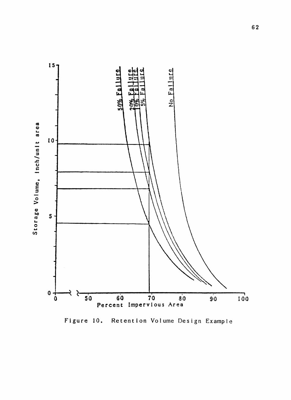
Read storage per unit area from Figure 10 at different values of percent failure.

Percent Storage from graph Storage Volume

FalIure (gallons/sq ft) (gallons)

5% 0.97 10,864

10% 0.79 8,848

20% 0.68 7,616

50% 0.47 5,264

62

I5n

CO

u c

93

E 3 O

>

V bo CO La

o CO

50 60 70 80 Percent Impervious Area

90 100

Figure 10. Retention Volume Design Example

APPENDIX C: ECONOMIC ANALYSIS

This appendix shows the unit prices and results of the

economic analysis for the cistern alternatives.

Formed-in-pI ace Concrete: Excavation d) $3.42/cy* Forms in place

Floor pad @ $6.15/sfsa Wal Is (D $6.50/sfsa CeiIing @ $9.25/sfsa

Reinforcing steel Floor pad - 3 Ib/cy @ $915/ton Walls - 24 Ib/cy @$930/ton Ceiling - 40 Ib/cy @ $1025/ton

Concrete (3000 psi) @ $54/cy Backfill - 12" lifts @$3.90/cy Asphalt coating (D $1.68/sfsa

•(Mahoney et al., 1985)

FibergI ass tank: Cost of tank

10,000 gal. @ $5050 8,000 gal. @ $4425 6,000 gal. @ $3795

Cost of shipment @ $800/16,000 gal. Excavation @ $3.42/cy BackfI I 1 @ $3.90/cy Peagravel for fill @ $17/cy delivered

•(XERXES Corp., telephone conversation)

Comparison of Alternatives Size of Ci s tern

Cistern 6,000 8,000 10.000 Al ternat Ive gal Ions gal Ions FJ l Ions

Formed-i n-pI ace Concrete $8,325 $10,426 $12,246

Flberg lass Tank $5,013 $6,390 $7,337

63

64

1986 Water Rate Structure for Lubbock, Texas

First 1,000 gal. $5.46 (minimum) Next 49,000 gal. $1.13 /looO gal. Next 200,000 gal. $ .97 /lOOO gal. Over 250,000 gal. $ .91 /lOOO gal.

Average sprinkler use per dwelling = 186 gal/day = 67,890 gal/day

Average annual irrigation expense = 12(5.46) + [(76.89 -12)(1.13)1

= $128.68 per year

PERMISSION TO COPY

In presenting this thesis in partial fulfillment of the

requirements for a master's degree at Texas Tech University, I agree

that the Library and my major department shall make it freely avail­

able for research purposes. Permission to copy this thesis for

bcholatly purposes luay be granted by the Director of the Library or

my major professor. It is understood that any copying or publication

of this thesis for financial gain shall not be allowed without my

further written permission and that any user may be liable for copy­

right infringement.

Disagree (Permission not granted) Agree (Permission granted)

A d/J^ UJjL^ Student's signature Student's signature

Date Date