SASEG 6B Introduction to Analysis of Variance (ANOVA)
22
SASEG 6B – Introduction to Analysis of Variance (ANOVA) (Fall 2015) Sources (adapted with permission)- T. P. Cronan, Jeff Mullins, Ron Freeze and David E. Douglas Course and Classroom Notes Enterprise Systems, Sam M. Walton College of Business, University of Arkansas, Fayetteville Microsoft Enterprise Consortium IBM Academic Initiative SAS ® Multivariate Statistics Course Notes & Workshop, 2010 SAS ® Advanced Business Analytics Course Notes & Workshop, 2010 Microsoft ® Notes Teradata ® University Network For educational uses only - adapted from sources with permission. No part of this publication may be reproduced, stored in a retrieval system, or transmitted, in any form or by any means, electronic, mechanical, photocopying, or otherwise, without the prior written permission from the author/presenter.
Transcript of SASEG 6B Introduction to Analysis of Variance (ANOVA)

SASEG 6B – Introduction to Analysis of Variance (ANOVA)
(Fall 2015)
Sources (adapted with permission)-
T. P. Cronan, Jeff Mullins, Ron Freeze and David E. Douglas Course and Classroom Notes
Enterprise Systems, Sam M. Walton College of Business, University of Arkansas, Fayetteville
Microsoft Enterprise Consortium
IBM Academic Initiative
SAS® Multivariate Statistics Course Notes & Workshop, 2010
SAS® Advanced Business Analytics Course Notes & Workshop, 2010
Microsoft® Notes
Teradata® University Network
For educational uses only - adapted from sources with permission. No part of this publication may be
reproduced, stored in a retrieval system, or transmitted, in any form or by any means, electronic,
mechanical, photocopying, or otherwise, without the prior written permission from the author/presenter.

2
One-Way ANOVA
Analysis of variance (ANOVA) is a statistical technique used to compare the means of two or more
groups of observations or treatments. For this type of problem, you have a
continuous dependent variable, or response variable
discrete independent variable also called a predictor or explanatory variable.
20
Objectives Analyze differences between population means
using the Linear Models task.
Verify the assumptions of analysis of variance.
20
21
OverviewAre there any differences among the population means?
21
Response
Continuous
Predictor
Categorical
One-Way
ANOVA

3
A t-test can be thought of as a special case of ANOVA: if you analyze the difference between means
using ANOVA, you get the same results as with a t-test. It just looks different in the output. Performing a
two-group mean comparison test in the Linear Models task gives you access to different graphical and
assessment tools than performing it in the t Test task.
When there are three or more levels for the grouping variable, a simple approach is to run a series of
t-tests between all the pairs of levels. For example, you might be interested in T-cell counts in patients
taking three medications (including one placebo). You could simply run a t-test for each pair of
medications. A more powerful approach is to analyze all the data simultaneously. The model is the same,
but it is now called a one-way analysis of variance (ANOVA), and the test statistic is the F ratio, rather
than the Student’s t value.
22
Research Questions for One-Way ANOVADo accountants, on average, earn more than teachers?*
*Isn’t this a case for a t-test?
22
23
Research Questions for One-Way ANOVADo people treated with one of two new drugs have higher
average T-cell counts than people in the control group?
23
Placebo Treatment 1
Treatment 2

4
24
Research Questions for One-Way ANOVADo people spend different amounts depending on which
type of credit card they have?
24
25
Research Questions for One-Way ANOVADoes the type of fertilizer used affect the average weight
of garlic grown at the Montana Gourmet Garlic ranch?
25

5
Example: Christin and Nicole own Montana Gourmet Garlic, a company that grows garlic using
organic methods. They specialize in hardneck varieties. Knowing a little about experimental
methods, they design an experiment to test whether growth of the garlic is affected by the type
of fertilizer used. They limit their experimentation to a Rocambole variety called Spanish
Roja. They test three different organic fertilizers and one chemical fertilizer (as a control).
They blind themselves to the fertilizer (in other words, they design the experiment in such a
way that they do not even know which fertilizer is in which container) by using containers with
numbers 1 through 4. One acre of farmland is set aside for the experiment. It is divided into
32 beds. They randomly assign fertilizers to beds. At harvest, they calculate the average
weight of garlic bulbs in each of the beds. The data is in the MGGarlic data set.
The variables in the data set are
Fertilizer The type of fertilizer used (1 through 4)
BulbWt The average garlic bulb weight (in pounds) in the bed
Cloves The average number of cloves on each bulb
BedID A randomly assigned bed identification number
26
Garlic Example
26

6
Exercise - Descriptive Statistics across Groups
Obtain summary statistics and a box and whisker plot for the MGGARLIC data set.
1. Open the MGGARLIC data set.
2. Select Tasks Describe Summary Statistics….
3. Select BulbWeight as the analysis variable and Fertilizer as the classification variable.
4. Under Plots, check Box and whisker.
7
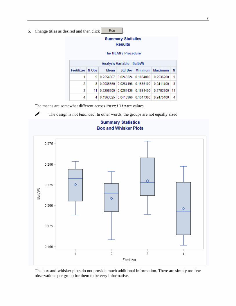
5. Change titles as desired and then click .
The means are somewhat different across Fertilizer values.
The design is not balanced. In other words, the groups are not equally sized.
The box-and-whisker plots do not provide much additional information. There are simply too few
observations per group for them to be very informative.

8
Small differences between sample means are usually present. The objective is to determine whether these
differences are significant. In other words, is the difference more than what might be expected to occur by
chance?
The assumptions for ANOVA are
independent observations
normally distributed error for each treatment
equal error variances across treatments.
28
The ANOVA Hypothesis
28
H0: F1=F2=F3=F4H1: F1 ≠ F2 or F1 ≠ F3
or F1 ≠ F4 or F2 ≠ F3
or F2 ≠ F4 or F3 ≠ F4

9
In ANOVA, the corrected total sum of squares is partitioned into two parts, the Model Sum of
Squares and the Error Sum of Squares.
Model Sum of Squares (SSM) the variability explained by the independent variable and therefore
represented by the between treatment sums of squares.
Error Sum of Squares (SSE) the variability not explained by the independent variable. Also
referred to as within treatment variability or residual sum of
squares.
Total Sum of Squares (SST) the overall variability in the response variable.
SST=SSM + SSE.
29
Partitioning Variability in ANOVA
29
Total
Variability
Variability
between GroupsVariability
within Groups

10
As its name implies, analysis of variance analyzes the variances of the data to determine whether there is
a difference between the group means. ANOVA compares the portion of variation in the response variable
attributable to the grouping variable to the portion of variability left unexplained. Another way to say this
is that ANOVA compares the sample variance under the null and alternative hypotheses.
Between Group Variation the weighted (by group size) sum of the squared differences between the
mean for each group and the overall mean, 2YYn ii . This measure is
also referred to as the Model Sum of Squares (SSM).
Within Group Variation the sum of the squared differences between each observed value and the
mean for its group, 2iij YY . This measure is also referred to as the
Error Sum of Squares (SSE).
Total Variation the sum of the squared differences between each observed value and the
overall mean, 2YYij . This measure is also referred to as the
Total Sum of Squares (SST).
30
Sums of Squares
30
Total
Variation
(SST)Within Group
Variation
(SSE)
Between Group
Variation (SSM)

11
The model, Yik = + I + ik, is just one way of representing the relationship between the dependent
and independent variables in ANOVA.
Yik the kth value of the response variable for the ith treatment.
the overall population mean of the response, for instance garlic bulb weight.
i the difference between the population mean of the ith treatment and the overall mean, . This
is referred to as the effect of treatment i.
ik the difference between the observed value of the kth observation in the ith group and the mean
of the ith group. This is called the error term.
SAS uses a parameterization of categorical variables that will not directly estimate the values
of the parameters in the model shown.
The researchers are interested only in these four specific fertilizers. In some references this would
be considered a fixed effect, as opposed to a random effect. Random effects are not covered in this
course.
35
The ANOVA Model
35
Yik = + i + ik
BulbWt = + + Base
LevelFertilizer
Unaccounted
for Variation

12
ANOVA Assumptions
The validity of the p-values depends on the data meeting the assumptions for ANOVA. Therefore, it is
good practice to verify those assumptions in the process of performing the analysis of group differences.
Independence implies that the ijs in the theoretical model are uncorrelated. The independence assumption
should be verified with good data collection. In some cases, residuals can be used to verify this
assumption.
The errors are assumed to be normally distributed for every group or treatment.
One assumption of ANOVA is approximately equal error variances for each treatment. Although you can
get an idea about the equality of variances by looking at the descriptive statistics and plots of the data, you
should also consider a formal test for homogeneity of variances. The SAS code has a homogeneity of
variance test option for one-way ANOVA.
36
Assumptions for ANOVA
36
Observations are independent.
Errors are normally distributed.
All groups have equal response variances.

13
37
The Linear Models Task
37
38
Assessing ANOVA Assumptions Good data collection methods help ensure the
independence assumption.
Diagnostic plots can be used to verify the assumption
that error is approximately normally distributed.
The Linear Models task produces a hypothesis test to
check for equal variances. H0 for this hypothesis test
is that the variances are equal for all populations.
38

14
The residuals from the ANOVA are calculated as (the actual value – the predicted value). These residuals
can be examined with the Distribution Analysis task to determine normality. With a reasonably sized
sample and approximately equal groups (balanced design), only severe departures from normality are
considered a problem. Residual values sum to 0 in ANOVA. Their distribution approximates the
distribution of error in the model.
In ANOVA with more than one predictor variable, homogeneity of variance test options are unavailable.
In those circumstances, you can plot the residuals against their predicted values to verify that the
variances are equal. The result will be a set of vertical lines equal to the number of groups. If the lines are
approximately the same height, the variances are approximately equal. Descriptive statistics can also be
used to determine whether the variances are equal.
39
Predicted and Residual ValuesThe predicted value in ANOVA is the group mean.
A residual is the difference between the observed value
of the response and the predicted value of the response
variable.
39

15
Exercise - The Linear Models task
Perform ANOVA to test whether the mean bulb weight of garlic is different across different
fertilizers.
1. Click the Input Data tab of the task flow to expose the MGGARLIC data set.
2. Select Tasks (or Analyze) ANOVA Linear Models….
3. Under Data, assign BulbWeight and Fertilizer to the task roles of dependent variable and
classification variable, respectively.

16
4. Under Model, click Fertilizer and then click .
The Class and quantitative variables pane was populated by the selection
of task roles.

17
5. Under Model Options, uncheck Type I and Show parameter estimates.
6. Click .
Turn your attention to the first page of the output, which specifies the number of levels and the values of
the class variable, and the number of observations read versus the number of observations used. These
values are the same because there are no missing values for any variable in the model. If any row has
missing data for a predictor or response variable, that row is dropped from the analysis.

18
The second page of the output contains all of the information that is needed to test the equality of the
treatment means. It is divided into three parts:
the analysis of variance table
descriptive information
information about the class variable in the model
Look at each of these parts separately.
In general, degrees of freedom (DF) can be thought of as the number of independent pieces of
information.
Model DF is the number of treatments minus 1.
Corrected total DF is the sample size minus 1.
Error DF is the sample size minus the number of treatments (or the difference between the corrected
total DF and the Model DF.
Mean squares are calculated by taking sums of squares and dividing by the corresponding degrees of
freedom. They can be thought of as variances.
Mean square for error (MSE) is an estimate of 2, the constant variance assumed for all treatments.
If i = j, for all i j, then the mean square for the model (MSM) is also an estimate of 2.
If i j, for any i j, then MSM estimates 2 plus a positive constant.
MSE
MSMF .
Variance is the traditional measure of precision. Mean Square Error (MSE) is the traditional
measure of accuracy used by statisticians. MSE is equal to variance plus bias-squared. Because
the expected value of the sample mean x equals the population mean (), MSE equals the
variance.
Based on the above, if the F statistic is significantly larger than 1, it supports rejecting the null hypothesis,
concluding that the treatment means are not equal.

19
The F statistic and corresponding p-value are reported in the analysis of variance table. Because the
reported p-value (0.1432) is greater than 0.05, you conclude that there is no statistically significant
difference between the means.
The coefficient of determination, R2, denoted in this table as R-Square, is a measure of the proportion of
variability explained by the independent variables in the analysis. This statistic is calculated as
SST
SSMR 2
The value of R2 is between 0 and 1. The value is
close to 0 if the independent variables do not explain much variability in the data
close to 1 if the independent variables explain a relatively large proportion of variability in the data.
Although values of R2 closer to 1 are preferred, judging the magnitude of R2 depends on the context of the
problem.
The coefficient of variation (denoted Coeff Var) expresses the root MSE (the estimate of the standard
deviation for all treatments) as a percent of the mean. It is a unitless measure that is useful in comparing
the variability of two sets of data with different units of measure.
The BulbWt Mean is the mean of all of the data values in the variable BulbWt without regard to
Fertilizer.
Some interpret the R2 value as the “proportion of variance accounted for by the model”. Therefore, one
might say that in this model, Fertilizer explains about 17% of the variability of BulbWt.
For a one-way analysis of variance (only one classification variable), the information about the class
variable in the model is an exact duplicate of the model line of the analysis of variance table.
It is good practice to look at your diagnostic plots to check for the validity of your ANOVA
assumptions. The rest of the output is dedicated to verifying those statistical assumptions for
inference tests.

20
The graph above is a mosaic of plots having to do with residuals from the ANOVA model. You will focus
on the left three in this analysis.
The plot at the upper left is a Residual by Predicted plot. Essentially, you are looking for a random scatter
within each group. Any patterns or trends in this plot can indicate model assumption violations.
To check the normality assumption, look at the Quantile-Quantile plot at center left. There appears to be
no severe departure from normality because the observations all lie close to the diagonal reference line.
This conclusion is not contradicted by the residual histogram at the lower left.

21
46
Steps for ANOVA SummaryNull Hypothesis: All means are equal.
Alternative Hypothesis: At least one mean is different
from another.
1. Produce descriptive statistics.
2. Verify assumptions.
– Independence
– Errors are normally distributed
– Variances are equal for all groups
3. Examine the p-value on the ANOVA table. If the
p-value is less than alpha, reject the null hypothesis.
46

22
Another Exercise
1. Analyzing Data in a Completely Randomized Design
Consider an experiment to study four types of advertising: local newspaper ads, local radio ads,
in-store salespeople, and in-store displays. The country is divided into 144 locations, and 36 locations
are randomly assigned to each type of advertising. The level of sales is measured for each region in
thousands of dollars. You want to see whether the average sales are significantly different for various
types of advertising.
The ads data set contains data for these variables:
Ad type of advertising
Sales level of sales in thousands of dollars
a. Examine the data using the Summary Statistics task. What information can you obtain from
looking at the data?
b. Test the hypothesis that the means are equal. Be sure to check that the assumptions of the analysis
method you choose are met. What conclusions can you reach at this point in your analysis?