SAR Imaging of Moving Targets via Compressive Sensing

8/10/2019 SAR Imaging of Moving Targets via Compressive Sensing

http://slidepdf.com/reader/full/sar-imaging-of-moving-targets-via-compressive-sensing 1/13

1

SAR Imaging of Moving Targets via Compressive Sensing

Jun Wang, Gang Li, Hao Zhang, Xiqin Wang

Department of Electronic Engineering, Tsinghua University, Beijing 100084, China

Emails: [email protected], {gangli, haozhang, wangxq_ee}@tsinghua.edu.cn

Abstract

An algorithm based on compressive sensing (CS) is proposed for synthetic aperture radar (SAR) imaging of moving

targets. The received SAR echo is decomposed into the sum of basis sub-signals, which are generated by discretizing the

target spatial domain and velocity domain and synthesizing the SAR received data for every discretized spatial position and

velocity candidate. In this way, the SAR imaging problem is converted into sub-signal selection problem. In the case that

moving targets are sparsely distributed in the observed scene, their reflectivities, positions and velocities can be obtained by

using the CS technique. It is shown that, compared with traditional algorithms, the target image obtained by the proposed

algorithm has higher resolution and lower side-lobe while the required number of measurements can be an order of

magnitude less than that by sampling at Nyquist sampling rate. Moreover, multiple targets with different speeds can be

imaged simultaneously, so the proposed algorithm has higher efficiency.

Index Terms

Synthetic Aperture Radar, Compressive Sensing, Moving Target

1.

Introduction

Synthetic aperture radar (SAR) has been widely used for stationary scene imaging via matched filtering and discrete

Fourier transform (DFT). Recently, moving target imaging has attracted much attention. However, the image of moving

targets in the observed scene may be displaced and blurred in the azimuth direction because of the motion of targets. Many

algorithms have been proposed to deal with this problem. One class of algorithms is based on the estimation of target motion

parameters [1-9], e.g., the Doppler rate and the Doppler frequency centroid which are related to the velocities along the range

and azimuth directions, respectively. Another class of algorithms combines data reformatting with high order Doppler history

analysis, i.e., the Keystone transform [10], the second Keystone transform [11] or the Doppler Keystone transform [12] is

used to correct the range cell migration of target, and then the time-frequency analysis [20] or polynomial phase analysis



2

[21-22] is used to compensate the high order terms in the Doppler history. All the algorithms above convert moving target

imaging problem to static target imaging problem by compensating the error caused by the target motion, and then the

algorithms for stationary scene imaging, e.g., the Range- Doppler algorithm, can be used for imagery formation. Since the

Range-Doppler algorithm is based on matched filtering and DFT, the resolutions of final image in the range and azimuth

directions are limited by the bandwidth of transmitted signal and the length of the synthetic aperture, respectively. And high

side-lobes arise due to the DFT window effect. Moreover, the required Nyquist-rate sampling may cause huge data amount to

achieve high resolution. In addition, in above algorithms it is needed to deal with different targets respectively when there are

multiple targets with different speeds.

Recently, the compressive sensing (CS) theory [13-15] has been used in a variety of areas for its excellent performance on

reconstruction of sparse signals. Consider an equation y =Φx , where x is an unknown k -sparse signal of length N

(k -sparse means that x has k large elements), Φ is a M N measurement matrix, and y is the measurement vector of

length M . The CS theory states that x can be reconstructed by ( log ) M O k N measurements with high probability [13-15].

CS has already been applied to SAR imaging of static targets [16-18]. However, the algorithms in [16-18] are not suitable for

SAR imaging of moving targets due to the motion-induced phase error.

In this paper, we propose an algorithm of SAR imaging of moving targets based on the CS technique. We use the matching

pursuit strategy to formulate the SAR imaging problem as a basis sub-signal selection problem, where the basis sub-signals

are produced by discretizing the extended target space (here the extended target space is defined as a four-dimensional

domain spanned by range and azimuth positions and range and azimuth velocities) and synthesizing the SAR data for every

discretized spatial position and velocity candidate in the extended target space. There are two assumptions we make here.

First, all targets maintain uniform motion in the observation time. Second, the discretized target space is sparse, i.e., the

number of targets is much less than the size of discretized target space. By using the CS technique, the spatial positions and

the velocities of the targets can be reconstructed with a relatively small number of random measurements. Compared with

traditional DFT-based algorithms of moving target imaging, the proposed algorithm can obtain higher resolution and lower

side-lobe with fewer measurements. Moreover, multiple targets with different speeds can be simultaneously imaged by using

our algorithm and thus the imaging efficiency can be improved.

The remainder of this letter is organized as follows. The SAR signal model of moving targets is discussed in Section 2. The

proposed algorithm is formulated in Section 3. Numerical examples are provided in Section 4.



3

Notation: Vectors and matrices are denoted by boldface letters; all vectors are column vectors; ( )T denotes the transpose

operation;1

and2

denotes l 1 and l 2 norms, respectively; ( )vec generates a column vector by stacking the columns of a

matrix one underneath the other in sequence, e.g., for a M × N matrix X,

2nd column of1st column of th column of

(1,1), (2,1), , ( ,1), (1,2), (2,2), , ( ,2), , (1, ), (2, ), , ( , )

T vec

N

M M N N M N

XX X

X X X X X X X X X X

2.

SAR signal model of moving targets

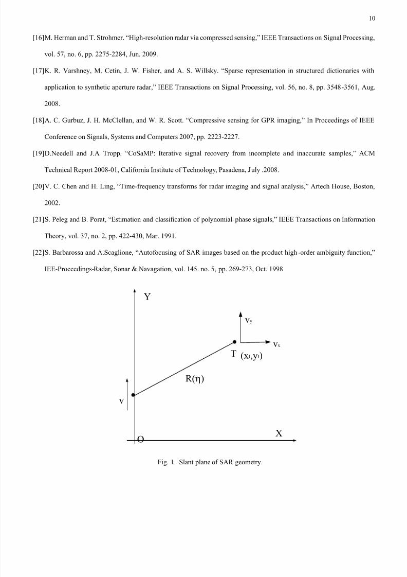
The typical side-looking SAR geometry is illustrated in Fig. 1. X -axis and Y -axis are range and azimuth directions,

respectively. The radar platform flies along Y -axis with constant speed v , and a point target T moves with constant range

speed xv and azimuth speed

yv , which lies in ( , )t t x y at 0 , here is the azimuth time (or slow time). Suppose that the

radar platform lies in (0,0) at 0 .

Assume that the radar transmits a chirp signal, then the baseband echo from T is:

2

0( , ) ( , ) ( 2 ( ) ) ( ) exp[ ( 2 ( ) ) ] exp[ 4 ( ) ]t t t t r a c r b s R c j K R c j f R c , (1)

where is the range time (or fast time),r

is the range envelope which is determined by the transmitted signal, anda

is

the azimuth envelope which is determined by the beam of the radar antenna,0 f is the carrier frequency,

t is the reflectivity

of T, ( , )t s corresponds to the received echo from a target which has the same position and speed with T while the

reflectivity is 1.c is the zero-Doppler time of the target which can be expressed as t

c

y

y

v v

, ( ) R is the instantaneous

distance from the radar to the target and it can be expressed as

2 2( ) ( ) ( ( ) )t x t y

R x v y v v , (2)

An approximate expression of (2) can be obtained by using the first two terms in the Taylor expansion atc :

2

2( )

( ) ( ) ( )2

y

t x c c

t

v v

R x v x

, (3)

We perform range compression on (1) and then the signal can be expressed as

2

20( )4

( , ) ( 2 ( ) ) ( ) exp{ [ ( ) ( ) ]}2

y

rc t r a c t x c c

t

v v f b p R c j x v

c x

, (4)

where ( )r p denotes the profile of the range-compressed signal, for example, ifr

is a rectangular envelope, thenr

p is a



4

sinc function.

It is clear that, 1) the range cell migration may occur if the variance of ( ) R during the observation duration is larger than

the range resolution; 2) the last term of the phase in (4) induces the time-varying Doppler frequency and will cause the final

image blurred. The goal of motion compensation is to correct both of the range cell migration and the time-varying Doppler

frequency. Once this is done, the focused image of the target can be directly obtained by performing the Fourier transform in

terms of .

From (1) we can express the SAR echo from the observed scene as

,( , ) ( , ) ( , ) x yb x y s dxdy , (5)

where ,( , )

x y s is the received echo from the target with reflectivity 1 located at ( , ) x y when 0 (see(1)), ( ) denotes

the reflectivities of possible targets. That is to say, if there is a target located at ( , ) x y when 0 , ( , ) x y denotes the

reflectivity of this target; if there is no target at the position ( , ) x y when 0 , ( , ) 0 x y . Here, we define ( ) as

reflectivity profile. In (5) ( , ) x y constitutes the target spaceT

which lies in the product space [ , ] [ , ]i f i f

x x y y . Here

( , )i i x y and ( , ) f f x y denotes the initial and final positions of the target space of interest along each axis, respectively. The

goal is to retrieve the profile ( ) that indicate the reflectivities and the positions of all possible targets (i.e., the image of the

target space) using the measurements ( , )b .

Normally we work with the discrete version of (5). If the measurements and the image (i.e., the reflectivity profile ( ) ) can

be expressed as vectors, a discretized reflectivity profile σ is related to the sampled measurement vector b through a matrix.

However, ,( , )

x y s can not be determined because the speed of the target located at ( , ) x y is unknown. A method to solve

this problem is to increase the dimensions of the target space. Consider the extended target space ,T e which lies in the

product space , , , ,[ , ] [ , ] [ , ] [ , ]i f i f x i x f y i y f x x y y v v v v . Here , ,( , )

x i y iv v and , ,( , )

x f y f v v denotes the minimum and maximum

velocity candidates of the extended target space along range and azimuth velocity axis, respectively. Thus the received echo

can be expressed as

, , ,( , ) ( , , , ) ( , ) x y x y x y v v x y

b x y v v s dxdydv dv , (6)

where ( ) is the reflectivity profile of the extended target space,, , ,

( , ) x y x y v v

s is the received echo from one target which is

located at ( , ) x y at 0 with reflectivity 1 and whose range and azimuth speeds are x

v and yv , respectively (see(1) and



5

(3)). From (1), (3) and (6) one can see that targets with different positions or speeds provide different contributions on the

measurements ( , )b , which implies that the moving target can be uniquely determined in the extended target space [5].

Once the energy distribution of the extended target space is obtained, the sub-space ( , ) x y and the sub-space ( , ) x yv v show

the positions and the velocities of all possible targets, respectively. In what follows, we describe how to recover the extended

target space ( , , , ) x y x y v v from the measurements ( , )b .

3. CS for SAR moving target imaging

First we discretize the extended target space ,T e as a four dimensional space of size

1 2 N N P Q , where1 2, , N N P and

Q are the numbers of discretized values of , , x x y v and y

v , respectively. The bin sizes of , , x x y v and y

v are , ,r a r and

a , respectively.

If motion parameters of a moving target match the coordinates 1 2( , , , )n n p q in the discretized extended target space, from

(2) we can directly obtain the distance from the radar to the target:

1 2

2 2

( , , , ) 1 2( ( ) ( ) ) ( ( ) ( ( ) ) )

n n p q x y R x n v p y n v q v , (7)

where1 1( ) i r x n x n ,

2 2( ) i a y n y n , ,( ) x x i r

v p v p , ,( ) y y i a

v q v q .

Suppose that the reflectivity of the target is 1, and then the baseband echo can be expressed as (see (1) and (6)):

1 2 1 2

1 2 1 2 1 2

( , , , ) ( ), ( ), ( ), ( )

2

( , , , ) ( , , , ) 0 ( , , , )

( , ) ( , )

( 2 ( ) ) ( ) exp[ ( 2 ( ) ) ] exp[ 4 ( ) ]

x yn n p q x n y n v p v q

r n n p q a c r n n p q n n p q

d s

R c j K R c j f R c

, (8)

We define (8) as the sub-signal corresponding to the coordinates1 2( , , , )n n p q . Thus, the SAR received echo of the

observed scene can be expressed as the sum of all sub-signals (see(6)):

1 2

1 2

1 2

1 1 11

1 2 ( , , , )

0 0 0 0

( , ) ( , , , ) ( , ) N N Q P

n n p q

n n p q

b a n n p q d

, (9)

where 1 2 1 2( , , , ) ( ( ), ( ), ( ), ( )) x ya n n p q x n y n v p v q . Suppose that 1 2

( , , , )a n n p q is the1 2( , , , )n n p q th element of a , and thus a

is a 1 2 N N P Q reflectivity profile matrix.

Assume that the range and azimuth sample rates are s

f anda

f respectively, the range and azimuth sample numbers are

r N and

a N respectively. Thus, the SAR received echo can be discretized as a

r a N N matrix, and its ( , )m n th element is

1 2

1 2

1 2

1 1 11

1 2 ( , , , )

0 0 0 0

( , ) ( , , , ) ( , ) N N Q P

m n n n p q m n

n n p q

b a n n p q d

, (10)



6

where0

/m s

m f , /n a

n f ,0

/ (2 )i

x c .

Let b isr a

N N matrix whose ( , )m n th element is ( , )m n

b , and let1 2( , , , )n n p q

d is ar a

N N matrix whose ( , )m n th

element is1 2( , , , ) ( , )n n p q m nd . Vectorize all

1 2( , , , )n n p qd for n1=0, … , N 1-1, n2=0, … , N 2-1, p=0, … , P -1, q=0, … ,Q-1 and

arrange all of them as a matrix Φ :

1 2 1 2(0,0,0,0) ( , , , ) ( 1, 1, 1, 1)[ , , , , ]vec vec vec

n n p q N N P Q Φ d d d , (11)

where1 2( , , , )

vec

n n p qd is a vector of length

r a N N , which is the vectorization of1 2( , , , )n n p q

d , Φ is a1 2r a

N N N N PQ matrix. Thus (9)

can be expressed as

vec vec b Φ a , (12)

where veca and vec

b are vectorizations of a and b , whose sizes are1 2 1 N N PQ and 1r a N N , respectively. All

1 2( , , , )

vec

n n p qd for

n1=0, … , N 1-1, n2=0, … , N 2-1, p=0, … , P -1, q=0, … ,Q-1, are called sub-signals, and thus the solution of (12) can be

considered as the sub-signal selection problem, which can be solved by the CS technique.

According to the CS theory [13-15], if veca is a k-sparse vector,

1 2[ log( )] M O k N N PQ measurements are enough to

reconstruct veca . Consider |vec

M b as randomly selected M elements of vecb , i.e., the mth element of |vec

M b is them

th

element of vecb , where

m are integers for 1,2, ,m M and

1 21 M r a N N . |

M Φ means a

1 2 M N N PQ

matrix whose mth row is them

th row of Φ . Then by randomly selecting M elements from vecb and corresponding M rows

from Φ , (12) can be rewritten as

| |vec vec

M M b Φ a , (13)

which can be solved by

minimize1

veca , subject to

2| |vec vec

M M b Φ a , (14)

where is the error threshold. The solution (14) can be obtained by using the CoSaMP algorithm [19]. Then the reflectivity

profile a can be obtained. Thus the correct sub-signals that really contribute to the received SAR echo are selected and the

projection coefficients of the SAR echo on these sub-signals are solved. The positions and reflectivities of the targets directly

represent the SAR final image, and meanwhile the velocities of the targets are also known. It is clear that1 2k N N since the

observed scene is sparse, and in general N 1 N 2< N r N a, thusr ak N N .

1 2[ log( )] M O k N N PQ , sor a

M N N which means

the measurements in the proposed algorithm are much fewer than that in the traditional algorithm.



7

4. Numerical Examples

In this section, we use simulated data to verify the feasibility and effectiveness of the proposed algorithm. Parameters of

the SAR system are shown in Table I. The size of the observed scene is 15m 15m , and the velocity in each direction is

limited in (-10m/s,10m/s) . The bins of the dimensions of the extended target space are 0.5m, 0.5m, 2m/s and 2m/s,

respectively, i.e., 0.5mr a

, 2m/sr a , and thus the extended target space is a 31 31 11 11 four-dimensional

space, i.e.,1 2 31 N N , 11 P Q . The radar platform transmits chirp signal and suppose that the range and azimuth

envelopes are both rectangular envelopes.

A. Feasibility

Suppose that there are three targets with reflectivity 1 in the observed scene. The first target is static, the second one is

moving along range direction with speed 10m/s, and the third one is moving with range speed 4m/s and azimuth speed 4m/s.

When 0 , the three target are located in (4m, 2.5m), (7.5m, 10m) and (11.5m, 8m) as illustrated in Fig. 2(a).

Firstly, the imaging result by the traditional algorithm is shown. The range sample number 1213r

N and the azimuth

sample number 595a N , so the measurement number of the traditional algorithm is N r N a=721735. The motion parameters

of the three targets are estimated by the range cell migration correction and the high order Doppler phase compensation as

done in [12]. Then the imaging result of the Range-Doppler algorithm is illustrated in Fig. 2(b). We can see that the image is

blurred due to the poor resolution and the high side-lobe.

Then the imaging result by the proposed algorithm is shown. Randomly select =100 M measurements from the SAR echo

vecb , and then solve (14) using the CoSaMP algorithm [19]. The imaging result is illustrated in Fig. 2(c). Compared with Fig.

2(b), the resolution is significantly improved and the side-lobe is removed, meanwhile the measurements are reduced from

721735 to 100. Another point to note is that the traditional algorithm [12] needs to estimate motion parameters of each target

one by one for above three targets. Thus, the proposed algorithm is more efficient in the case of multiple targets with different

velocities.

B. Ef fect of the number of measurements

An important measure of CS technique is the successful recovery probability, plotted in Fig. 3 as a function of the number

of measurements for a varying number of targets (sparsity level P ), i.e., 1-4. The positions and speeds of targets in the

observed scene are randomly generated. For each point on the plot, 200 trials of the proposed algorithm are run. Suppose that



8

ˆvec

a is the solution of the reflectivity profile veca by (14), then if

2 2ˆ 0.1vec vec vec a a a , the image is counted as a

successful recovery. The number of successful recoveries over 200 trials yields the probability of successful recovery (PSR)

in terms of the measurement and the sparsity level P . It can be observed that increasing the sparsity level P , i.e., the number

of targets, requires more measurements for the same level of PSR. Moreover, even for P =4, 60 measurements are enough to

achieve high PSR, which is still far less than the 721735 measurements needed for traditional algorithms.

C. Ef fect of the noise

To analyze the effect of versus (additive) noise level, the algorithm is applied to the received SAR data with SNRs from -15

to 35dB. The number of the targets is 1 whose position and speed are generated randomly. Fig. 4 shows the PSR as a function

of SNR for varying number of measurements. For each point on the plot, 100 trials of the proposed algorithm are run. It can

be observed that increasing the number of measurements allows the method to perform at lower SNR values. Even with small

number of measurements, i.e., 20, high successful recovery rates can be obtained with SNRs more than 15dB.

5. Conclusion

This paper proposes a CS-based algorithm for SAR imaging of moving targets. The received SAR echo is decomposed as

the sum of many basis sub-signals that are generated by discretizing the target spatial domain and velocity domain and

synthesizing the SAR received data for every discretized spatial position and velocity candidate. By using the CS technique,

the correct sub-signals that contribute to the received SAR echo are selected and the projection coefficients of the SAR echo

on these sub-signals are solved. The positions and reflectivities of the targets directly represent the SAR final image, and

meanwhile the velocities of the targets are also obtained. Numerical examples show that, compared with traditional

algorithms based on Doppler phase analysis and DFT, the proposed algorithm can obtain better imagery quality with higher

resolution and lower side-lobe. Moreover, the measurements used by the proposed algorithm are much fewer. In addition,

multiple targets with different velocities can be imaged simultaneously and thus the proposed algorithm has higher

efficiency.

References

[1] S. Werness, W. Carrara, L. Joyce, and D. Franczak, “Moving target imaging algorithm for SAR data,” IEEE

Transactions on Aerospace and Electronic Systems, vol.26, no.1, pp. 57-67, Jan.1990.



9

[2] M. Kirscht, “Detection and imaging of arbitrarily moving targets with single-channal SAR,” IEE Proceedings - Radar,

Sonar & Naigation, vol.150, no.1, pp.7-11, Feb.2003.

[3]

P.A.C. Marques and J.M.B. Dias, “Velocity estimation of fast moving targets using a single SAR sensor,” IEEE

Transactions on Aerospace and Electronic Systems, vol.41, no.1, pp. 75-89, Jan.2005.

[4]

P.A.C. Marques and J.M.B. Dias, “Moving target processing in SAR spatial domain,” IEEE Transactions on Aerospace

and Electronic Systems, vol.43, no.3, pp. 864-874,Jul.2007.

[5] G. Li, X.-G. Xia, J. Xu, and Y.- N. Peng, “A velocity estimation algorithm of moving targets using single antenna SAR ,”

IEEE Transactions on Aerospace and Electronic Systems, vol.45, no.3, pp. 1052-1062,Jul.2009.

[6] S. Barbarossa, “Detection and imaging of moving objects with synthetic aperture radar,” IEE Proceedings -.F, vol.139,

no.1, pp.79-97, Feb.1992.

[7]

M. Soumekh, “Reconnaissance with ultra wideband UHF synthetic aperture radar,” IEEE Signal Processing Magazine,

vol. 12, no.4, pp.21-40, Jul.1995.

[8] V.C. Chen and L. Hao, “Joint time-frequency analysis for radar signal and image processing,” IEEE Signal Processing

Magazine, vol. 16, no. 2, pp.81-93, Mar. 1999

[9] G. Wang, X.-G. Xia, and V.C. Chen, “Dual-speed SAR imaging of moving targets,” IEEE Transactions on Aerospace

and Electronic Systems, vol.42, no.1, pp.368-379, Jan.2006.

[10]

R.P. Perry, R.C. Dipietro, and R.L. Fante, “SAR maging of moving targets,” IEEE Transaction on Aerospace and

Electronic Systems, vol.35, no.1, pp.188-200, Jan.1999.

[11] F. Zhou, R. Wu, M. Xing, and Z. Bao, “Approach for single channel SAR ground moving target imaging and motion

parameter estimation”, IET Radar, Sonar & Navigation, vol.1, no.1, pp.59-66, Feb.2007.

[12]

G. Li, X.-G. Xia, and Y.-N.Peng, “Doppler Keystone Transform for SAR imaging of moving Targets,” IEEE

Geoscience and Remote Sensing Letters, vol. 5, no. 4, pp. 573-577, Oct. 2008.

[13]

E.J. Candes, J. Romberg, and T. Tao, “Robust uncertanity principles: exact signal reconstruction from highly incomplete

frequency information,” IEEE Transactions on Information Theory, vol.52, pp. 489-509, 2006.

[14]

D.L.Donoho, “Compressive sensing,” IEEE Transactions on Information Theory, vol.52, no.4, pp. 1289-1306, 2006.

[15]

R. Baraniuk and P. Steeghs. “Compressive radar imaging,” In Proceedings of IEEE Radar Conference 2007, pp.

128-133.



10

[16] M. Herman and T. Strohmer. “High-resolution radar via compressed sensing,” IEEE Transactions on Signal Processing,

vol. 57, no. 6, pp. 2275-2284, Jun. 2009.

[17]

K. R. Varshney, M. Cetin, J. W. Fisher, and A. S. Willsky. “Sparse representation in structured dictionaries with

application to synthetic aperture radar,” IEEE Transactions on Signal Processing, vol. 56, no. 8, pp. 3548-3561, Aug.

2008.

[18] A. C. Gurbuz, J. H. McClellan, and W. R. Scott. “Compressive sensing for GPR imaging,” In Proceedings of IEEE

Conference on Signals, Systems and Computers 2007, pp. 2223-2227.

[19] D.Needell and J.A Tropp, “CoSaMP: Iterative signal recovery from incomplete and inaccurate samples,” ACM

Technical Report 2008-01, California Institute of Technology, Pasadena, July .2008.

[20] V. C. Chen and H. Ling, “Time-frequency transforms for radar imaging and signal analysis,” Artech House, Boston,

2002.

[21] S. Peleg and B. Porat, “Estimation and classification of polynomial- phase signals,” IEEE Transactions on Information

Theory, vol. 37, no. 2, pp. 422-430, Mar. 1991.

[22] S. Barbarossa and A.Scaglione, “Autofocusing of SAR images based on the product high -order ambiguity function,”

IEE-Proceedings-Radar, Sonar & Navagation, vol. 145. no. 5, pp. 269-273, Oct. 1998

Y

XO

v

vy

vx

T (xt,yt)

R()

Fig. 1. Slant plane of SAR geometry.



11

Range

A z i m u t h

0 5 10 15

0

5

10

150

0.1

0.2

0.3

0.4

0.5

0.6

0.7

0.8

0.9

1

(a)

Range

A

z i m u t h

0 5 10 15

0

5

10

15

0.1

0.2

0.3

0.4

0.5

0.6

0.7

0.8

0.9

1

(b)



12

Range

A z i m u t h

0 5 10 15

0

5

10

150

0.1

0.2

0.3

0.4

0.5

0.6

0.7

0.8

0.9

1

(c)

Fig. 2. (a)The observed scene; (b) The imaging result by the traditional DFT-based algorithm; (c) The imaging result by the

proposed algorithm.

0 10 20 30 40 50 60 70 800

0.2

0.4

0.6

0.8

1

M

P S R

P=1

P=2

P=3

P=4

Fig. 3 The probability of successful recovery (PSR) vs. the number of measurements ( M ) for varying number of targets ( P )

in the target space.



13

-15 -10 -5 0 5 10 15 20 25 30 350

0.2

0.4

0.6

0.8

1

SNR

P S R

M=20

M=40

M=100

M=200

Fig. 4 The probability of successful recovery (PSR) vs. SNR for varying number of measurements M

TABLE I

PARAMETERS OF THE SAR SYSTEM

Scene center range 30km Platform speed 250m/s

Pluse width

10us Carrier frequency 9.375GHz

Transmitted signal bandwidth 100MHz Antenna length 2m

Radar sampling rate 120MHz Radar wavelength 0.032m

Pulse repitition frequency 300Hz

SAR Imaging of Moving Targets via Compressive Sensing

Documents

Transcript of SAR Imaging of Moving Targets via Compressive Sensing