SALES FORECAST INACCURACY AND INVENTORY … · · 2010-07-15Usually a high turnover ratio...
68
SALES FORECAST INACCURACY AND INVENTORY TURNOVER PERFORMANCE: AN EMPIRICAL ANALYSIS OF U.S. RETAIL SECTOR A THESIS SUBMITTED TO THE DEPARTMENT OF INDUSTRIAL ENGINEERING AND THE INSTITUTE OF ENGINEERING AND SCIENCE OF BILKENT UNIVERSITY IN PARTIAL FULFILLMENT OF THE REQUIREMENTS FOR THE DEGREE OF MASTER OF SCIENCE By Gülşah Hançerlioğulları July, 2010
Transcript of SALES FORECAST INACCURACY AND INVENTORY … · · 2010-07-15Usually a high turnover ratio...

SALES FORECAST INACCURACY AND INVENTORY
TURNOVER PERFORMANCE: AN EMPIRICAL
ANALYSIS OF U.S. RETAIL SECTOR
A THESIS
SUBMITTED TO THE DEPARTMENT OF INDUSTRIAL
ENGINEERING
AND THE INSTITUTE OF ENGINEERING AND SCIENCE
OF BILKENT UNIVERSITY
IN PARTIAL FULFILLMENT OF THE REQUIREMENTS
FOR THE DEGREE OF
MASTER OF SCIENCE
By
Gülşah Hançerlioğulları
July, 2010

ii
I certify that I have read this thesis and that in my opinion it is full adequate, in scope
and in quality, as a dissertation for the degree of Master of Science.
___________________________________
Asst. Prof. Dr. Alper Şen (Advisor)
I certify that I have read this thesis and that in my opinion it is full adequate, in scope
and in quality, as a dissertation for the degree of Master of Science.
___________________________________
Prof. Dr. Nesim Erkip
I certify that I have read this thesis and that in my opinion it is full adequate, in scope
and in quality, as a dissertation for the degree of Master of Science.
______________________________________
Asst. Prof. Dr. Nagihan Çömez
Approved for the Institute of Engineering and Science
____________________________________
Prof. Dr. Levent Onural
Director of Institute of Engineering and Science
iii
ABSTRACT
SALES FORECAST INACCURACY AND INVENTORY
TURNOVER PERFORMANCE: AN EMPIRICAL ANALYSIS OF
U.S. RETAIL SECTOR
Gülşah Hançerlioğulları
M.S. in Industrial Engineering
Advisor: Asst. Prof. Dr. Alper Şen
July, 2010
We develop an empirical model to investigate the impact of various financial
measures on inventory turnover performance. In particular, we used inaccuracy of
quarterly sales forecasts as a proxy for demand uncertainty and study its impact on
firm level inventory turnover ratios. The model is implemented on a sample financial
data for 304 publicly listed U.S. retail firms for the 25-year period 1985-2009.
Controlling for the effects of retail sub-segments and year, it is found that inventory
turnover is negatively correlated with mean absolute percentage error in sales
forecast and gross margin, and positively correlated with capital intensity and sales
surprise. In addition to providing managerial insights regarding the determinants of a
major operational performance metric, our results can also be used to benchmark a
retailer’s inventory performance against its competitors.
Keywords: Inventory turnover, retail operations, sales forecast

iv
ÖZET
A.B.D PERAKENDE SEKTÖRÜNDE SATIŞ TAHMİN HATASI VE
ENVANTER DÖNÜŞ HIZI PERFORMANSININ AMPİRİK ANALİZİ
Gülşah Hançerlioğulları
Endüstri Mühendisliği, Yüksek Lisans
Tez Yöneticisi: Yrd. Doç. Dr. Alper Şen
Temmuz, 2010
Bu çalışmada, çeşitli finansal ölçütlerin envanter dönüş hızı performansı üzerindeki
etkisini araştırmak için ampirik model geliştirilmiştir. Özellikle, talepteki
belirsizliğini ifade etmek için çeyrek dönemlik satış tahminlerindeki hata kullanılıp,
bunun envanter dönüş hızına olan etkisi araştırılmıştır. 1985-2009 yılları arasında
Amerika Birleşik Devletleri’nde, halka açık, farklı sektörlerde yer alan 304 adet
perakende şirketinin finansal bilgileri incelendi. Perakende sektörü ve zamanın etkisi
kontrol edilerek, envanter dönüş hızının çeyrek dönemlik satış tahminlerindeki
ortalama mutlak hata ve brüt kâr oranı ile negatif; sermaye büyüklüğü ve sürpriz satış
terimiyle pozitif korelasyonu gözlenmiştir. Yönetimsel uygulamalara ışık tutmanın
yanı sıra; sonuçlarımız firmalar arası envanter performansını karşılaştırmak üzere de
kullanılabilir.
Anahtar Kelimeler: Envanter dönüş hızı, perakende operasyonları, satış tahmini

v
To my parents…

vi
Acknowledgement
First and foremost, I would like to express my sincere gratitude to my advisor Asst.
Prof. Dr. Alper Şen for his invaluable support, attention, guidance throughout the
study, as well as for his patience and insight.
I would like to extend my special gratitude to my dissertation committee, Prof. Dr.
Nesim Erkip and Asst. Prof. Dr. Nagihan Çömez for devoting their valuable time to
read and review this thesis and their substantial suggestions.
I would also like to thank my colleague and friend Esra Ağca from Virginia Tech for
working with us in this project and providing us the data.
I am deeply grateful to my family for their encouragement support and unbending
love not only throughout this study, but also throughout my life. I feel very lucky to
have such a wonderful family.
Many thanks to my friends Ardıç Çorapsız, Ece Demirci and Hatice Çalık for their
moral support and help during my graduate study. I am also thankful to my
officemates and classmates Pelin Damcı, Gökçe Akın, Korhan Aras, Yiğit Saç, Esra
Koca, Can Öz, Emre Uzun and all of friends I failed to mention here for their
friendship and support.

vii
TABLE OF CONTENTS
CHAPTER 1: INTRODUCTION .......................................................................................... 1
CHAPTER 2: LITERATURE REVIEW ................................................................................... 6
CHAPTER 3: DATA DESCRIPTION AND DEFINITION OF VARIABLES ..................... 10
CHATER 4: HYPOTHESIS DEVELOPMENT ...................................................................... 20
4.1. Gross Margin ................................................................................................................. 20
4.2. Capital Intensity ............................................................................................................ 21
4.3. Sales Surprise ................................................................................................................ 21
4.4. Mean Absolute Percentage Error in Sales Forecast ...................................................... 22
CHAPTER 5: EMPIRICAL MODEL ...................................................................................... 26
5.1. Model 1 ......................................................................................................................... 28
5.2. Model 2 ......................................................................................................................... 30
5.3. Model 3 ......................................................................................................................... 30
5.4. Model 4 ......................................................................................................................... 31
5.5. Model 5 ......................................................................................................................... 31

viii
CHAPTER 6: NUMERICAL ANALYSIS ............................................................................. 33
CHAPTER 7: CONCLUSION ................................................................................................ 52
ix
LIST OF FIGURES
Figure 1: Annual inventory turnover ratio vs. annual gross margin for four retailers .............. 3
Figure 2: The illustration of apparel and accessory stores ...................................................... 46
Figure 3: The illustration of catalog, mail-order houses ......................................................... 46
Figure 4: The illustration of department stores ....................................................................... 47
Figure 5: The illustration of drug and proprietary stores ........................................................ 47
Figure 6: The illustration of food stores.................................................................................. 48
Figure 7: The illustration of hobby, toy, and game shops....................................................... 48
Figure 8: The illustration of home furniture and equipment stores ........................................ 49
Figure 9: The illustration of jewelry stores ............................................................................. 49
Figure 10: The illustration of radio, TV, consumer electronics stores ................................... 50
Figure 11: The illustration of variety stores ............................................................................ 50

x
LIST OF TABLES
Table 1: Classification of Retail Segments ............................................................................. 11
Table 2: Notation .................................................................................................................... 13
Table 3: Notation for Holt’s method ....................................................................................... 15
Table 4: Summary statistics of the variables for each segment .............................................. 16
Table 5: Notation for Winter’s method .................................................................................. 17
Table 6: The best , and for each segment ..................................................................... 23
Table 7: The best , and for the some of the firms ......................................................... 24
Table 8: Models, Levels and Explanatory Variables .............................................................. 27
Table 9: Notation for the regression models ........................................................................... 29
Table 10: Coefficients’ Estimates for Model 1.1 .................................................................... 35
Table 11: Coefficients’ Estimates for Model 1.2 .................................................................... 35
Table 12: Coefficients’ Estimates for Model 1.3 .................................................................... 36
Table 13: Coefficients’ Estimates for Model 1.4 .................................................................... 36
Table 14: Coefficients’ Estimates for Model 2.1 .................................................................... 38
Table 15: Coefficients’ Estimates for Model 2.2 .................................................................... 38
Table 16: Coefficients’ Estimates for Model 2.3 .................................................................... 38
Table 17: Coefficients’ Estimates for Model 2.4 .................................................................... 38
xi
Table 18: Coefficients’ Estimates for Model 3.1 .................................................................... 40
Table 19: Coefficients’ Estimates for Model 3.2 .................................................................... 40
Table 20: Coefficients’ Estimates for Model 3.3 ................................................................... 41
Table 21: Coefficients’ Estimates for Model 3.4 .................................................................... 41
Table 22: Coefficients’ Estimates for Model 4.1 .................................................................... 43
Table 23: Coefficients’ Estimates for Model 4.2 .................................................................... 43
Table 24: Coefficients’ Estimates for Model 4.3 ................................................................... 43
Table 25: Coefficients’ Estimates for Model 4.4 ................................................................... 43
Table 26: Coefficients’ Estimates for Model 5.1 .................................................................... 44
Table 27: Coefficients’ Estimates for Model 5.2 .................................................................... 44
Table 28: Coefficients’ Estimates for Model 5.3 ................................................................... 44
Table 29: Coefficients’ Estimates for Model 5.4 ................................................................... 44

1
Chapter 1
INTRODUCTION
Inventories represent the stocks of raw materials, work-in process items and finished
goods that are kept to meet customer orders. Higher demand uncertainty, product
variety, and customer service levels put increased pressure on managers to increase
inventories. On the other hand, since 1980s, many changes in industry appear which
tend to reduce inventories such as improvements in information technology, adoption
of just-in-time, outsourcing, etc. Thus, keeping right levels of inventory is crucial in
order to meet customer commitments while minimizing cost.
Inventory turnover rate is the ratio of cost of goods sold to average inventory level. It
measures the number of times inventory sold or replaced in a period. Inventory
turnover ratio is perhaps the most widely used metric to measure a company’s
operational performance. Since inventory turnover ratio scales inventory to sales, it
can be used for evaluating performance progress over time and comparing the
inventory performance across the firms.
2
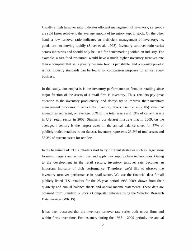
Usually a high turnover ratio indicates efficient management of inventory, i.e. goods
are sold faster relative to the average amount of inventory kept in stock. On the other
hand, a low turnover ratio indicates an inefficient management of inventory, i.e.
goods are not moving rapidly (Silver et al., 1998). Inventory turnover ratio varies
across industries and should only be used for benchmarking within an industry. For
example, a fast-food restaurant would have a much higher inventory turnover rate
than a company that sells jewelry because food is perishable, and obviously jewelry
is not. Industry standards can be found for comparison purposes for almost every
business.
In this study, our emphasis is the inventory performance of firms in retailing since
major fraction of the assets of a retail firm is inventory. Thus, retailers pay great
attention to the inventory productivity, and always try to improve their inventory
management processes to reduce the inventory levels. Gaur et al.(2005) state that
inventories represent, on average, 36% of the total assets and 53% of current assets
in U.S. retail sector in 2003. Similarly our dataset illustrate that in 2009, on the
average, inventory is the largest asset on the annual balance sheet for 57% of
publicly traded retailers in our dataset. Inventory represents 23.5% of total assets and
58.3% of current assets for retailers.
In the beginning of 1990s, retailers start to try different strategies such as larger store
formats, mergers and acquisitions, and apply new supply chain technologies. Owing
to the development in the retail sectors, inventory turnover rate becomes an
important indicator of their performance. Therefore, we’d like to observe the
inventory turnover performance in retail sector. We use the financial data for all
publicly listed U.S. retailers for the 25-year period 1985-2009, drawn from their
quarterly and annual balance sheets and annual income statements. These data are
obtained from Standard & Poor’s Compustat database using the Wharton Research
Data Services (WRDS).
It has been observed that the inventory turnover rate varies both across firms and
within firms over time. For instance, during the 1985 – 2009 periods, the annual
3
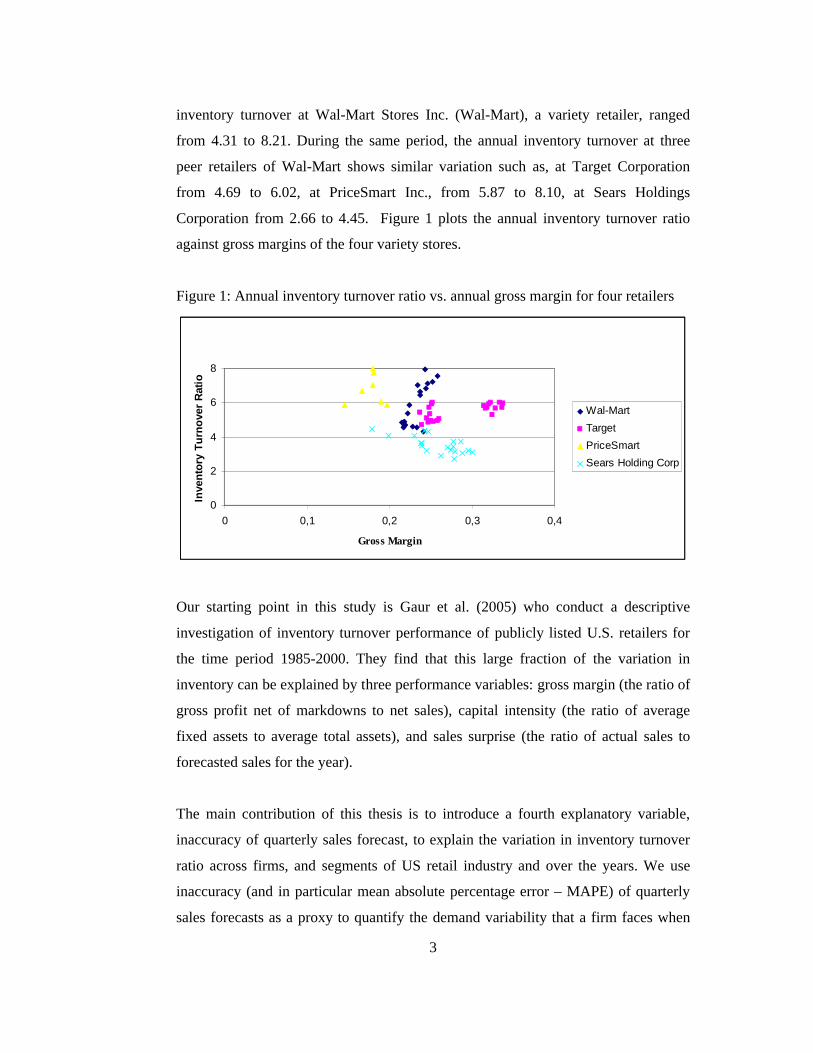
inventory turnover at Wal-Mart Stores Inc. (Wal-Mart), a variety retailer, ranged
from 4.31 to 8.21. During the same period, the annual inventory turnover at three
peer retailers of Wal-Mart shows similar variation such as, at Target Corporation
from 4.69 to 6.02, at PriceSmart Inc., from 5.87 to 8.10, at Sears Holdings
Corporation from 2.66 to 4.45. Figure 1 plots the annual inventory turnover ratio
against gross margins of the four variety stores.
Figure 1: Annual inventory turnover ratio vs. annual gross margin for four retailers
0
2
4
6
8
0 0,1 0,2 0,3 0,4
Gross Margin
Inve
nto
ry T
urn
ove
r R
atio
Wal-Mart
Target
PriceSmart
Sears Holding Corp
Our starting point in this study is Gaur et al. (2005) who conduct a descriptive
investigation of inventory turnover performance of publicly listed U.S. retailers for
the time period 1985-2000. They find that this large fraction of the variation in
inventory can be explained by three performance variables: gross margin (the ratio of
gross profit net of markdowns to net sales), capital intensity (the ratio of average
fixed assets to average total assets), and sales surprise (the ratio of actual sales to
forecasted sales for the year).
The main contribution of this thesis is to introduce a fourth explanatory variable,
inaccuracy of quarterly sales forecast, to explain the variation in inventory turnover
ratio across firms, and segments of US retail industry and over the years. We use
inaccuracy (and in particular mean absolute percentage error – MAPE) of quarterly
sales forecasts as a proxy to quantify the demand variability that a firm faces when

4
making inventory decisions and test the hypothesis that it as a significant impact on
annual inventory turnover ratios in retail firms. We use Winter’s triple exponential
smoothing method and apply it individually by optimizing its three parameters to
obtain the forecast for each firm. While forecast inaccuracy of quarterly sales of a
firm may not be a direct indication of the amount of demand variability that it is
exposed to its individual items due to aggregation, we use this measure in the
absence of detailed demand data. This thesis also extends the study in Gaur et al.
(2005) to a more recent and larger data set and tests to see whether the three
hypotheses in Gaur et al. (2005) prevail with this data. In addition, we also comment
on which retail firms operate successfully and which do not according to the
differences between actual inventory turnover rates and inventory turnover rates that
are predicted by the regression models that we develop.
The main results of this thesis are as follows. First, we show that mean absolute
percentage error in quarterly sales forecast is negatively correlated with inventory
turnover ratio in most of the retail segments. On the average, a 1% increase in MAPE
is associated with a 0.01% decrease in inventory turnover. Second, we re-test the
hypotheses in Gaur et al. (2005) regarding gross margin, capital intensity and sales
surprise on our real world data set and find that inventory turnover is negatively
correlated with gross margin, and positively correlated with capital intensity and
sales surprise. On the average, in our data set, a 1% increase in gross margin is
associated with a 0.34% decrease in inventory turnover (statistically significant at
p<0.00001). Moreover, a 1% increase in capital intensity is associated with a 0.21%
increase in inventory turnover, and a 1% increase in sales surprise is associated with
a 0.10% increase in inventory turnover. These results are consistent with those
obtained by Gaur et al. (2005). We believe that our study might be useful for retail
managers to assess inventory turnover performance across firms and for a firm over
time, and to benchmark it against the competing firms in industry.
The rest of this thesis is organized as follows. In Chapter 2, relevant literature is
summarized. Chapter 3 describes the data set and defines the performance variables
used throughout this thesis. In Chapter 4, our hypotheses to relate inventory turnover

5
with gross margin, capital intensity, sales surprise and mean absolute percentage
error in forecasts are presented. In Chapter 5, the empirical model is provided.
Following that, in Chapter 6, we provide the numerical analysis. A general
conclusion of the study is presented in Chapter 7.

6
Chapter 2
LITERATURE REVIEW
This chapter consists of a review of literature related to our study. The impacts of
operational changes on financial and operational performance have been studied
recently. Nevertheless, the numbers of empirical studies on these topics are scarce.
We begin with the study of Rajagopalan and Malhotra (2001) who study the trends in
materials, work-in process and finished-goods inventory ratios for the 20
manufacturing industries for the period 1961 to 1964. They find that in a majority of
industry sectors, raw material and work-in-process inventories decreased from 1961
to 1994. Yet, finished-goods inventories decreased in some industry sectors and
increased in some others but did not show any overall trend. Authors show that total
manufacturing inventory ratios improved at a higher rate during the pre-1980 period
as compared with post-1980 period.

7
Hendricks and Singhal (2003) report that supply chain glitches, which resulted in
production or shipment delays, decrease the shareholder value. Their results are
based on a sample of 519 supply chain glitches that were publicly announced during
1989-2000. It is observed that larger firms’ stock market reaction to supply chain
glitches is less negative, and firms with higher growth prospects experience a more
negative stock market reaction.
Hendricks and Singhal (2005) later examine the association between supply chain
glitches and operating performance measures such as net sales, cost, inventory, etc.
for the period of 1992-1999. Authors observe that these performance measures do
not improve at least two years after the glitch announcement; hence firms do not
recover quickly. It is determined that announcement of glitches are negatively
correlated with net sales, inventory performance, profitability.
Similar to the study of Rajagopalan and Malhotra (2001), in an attempt to understand
the trends in inventory levels for each of raw material inventory, work-in-process
inventory and finished-good inventory, Chen at al. (2005) examine the inventories of
publicly traded American manufacturing companies for the period 1981 to 2000.
Authors observe the decline in raw material and work-in-process inventories;
nevertheless, finished-goods inventory remained the same. As a result, majority of
manufacturing firms in the United States reduced their inventories. In addition, the
authors also find that firms with high inventories have poor long-term stock returns;
firms with low inventories have unusually good long-term stock performance.
Chen et al. (2007) investigate whether the inventory turnover for U.S. retailers and
wholesale firms have improved or not over the period from 1981 to 2004. They find
that the average inventory that the firms carry decrease in manufacturing and
wholesale firms, so wholesale firms increased their inventory turnover year by year.
On the other hand, until 1995, inventory turnover ratios of retail firms remain stable.
After 1995, retail firms started to improve the inventory turnover. Similar to Chen et
al. (2005), it is stated that if the inventory performance of a company is poorer than
the average, the firm has poor long-term stock market performance.
8
Boute et al. (2007) analyze differences in inventory turnover between manufacturing,
wholesale and retail sectors. They only consider the year 2004, since their study aims
to express cross-sectional differences. The data was extracted from Bel-First which
contains statistics on Belgian and Luxembourg companies. They find that type of
production process affects work-in process inventory. They further state that
inventory turnover is significantly higher in retailer than wholesale.
Rumyantsev and Netessine (2007) analyze the panel data of a sample of 722 firms
and find that better earnings are associated with responsive inventory management.
They find that firms operating with demand uncertainty, longer lead times, and
higher gross margins have larger inventories.
Aghazadeh (2009) presents the correlation between company’s annual inventory
turnover and its performance in retail industry. Using an empirical model, the author
finds that future stock performance could be predicted by an indicator, which is the
variance of annual inventory turnover of the firms. Various firms in different
segments are analyzed in terms of their inventory turnover ratios. The author
concludes that if managers are able to control inventory turnover, both stock
performance and management quality of firms’ are affected positively.
Our main motivation in this study is the paper by Gaur et al. (2005) who analyze the
inventory turnover performance in the retail industry. They use financial data for 311
publicly listed retail firms for the period 1985-2000. The correlation of inventory
turnover with gross margin, capital intensity and sales surprise are investigated. They
develop several empirical models to test and strengthen their hypotheses. The basic
results of their study are as follows: Inventory turnover is negatively correlated with
the gross margin, positively correlated with the capital intensity with some
exceptions, and positively correlated with the sales surprise. Time trends in inventory
turnover and adjusted inventory turnover are computed as well. They find that
inventory turnover in retailing industry declined from 1985-2000.
9
As an extension of the Gaur et al. (2005), Gaur and Kesavan (2007) observe the
impact of firm size and sales growth rate on inventory turnover performance in retail
industry. Authors find that inventory turnover is positively correlated with sales
growth rate and growth rate is correlated with firm size. They use the 353 publicly
listed retail firms for the period 1985-2003. Re-testing the hypotheses in Gaur et al.
(2005) with larger and recent data set, they further obtain consistent results with
Gaur et al. (2005), and demonstrate that inventory turnover is negatively correlated
with gross margin, positively correlated with capital intensity, and positively
correlated with sales surprise.
In most of these studies, the data typically used are obtained from the Standard &
Poor’s Compustat database, U.S. Census Bureau or LexisNexis.
Our main contribution in this study is to develop a metric to quantify the sales
forecast inaccuracy that a firm faces and use this metric to understand the impact of
demand variability on that firm’s inventory turnover performance. In particular, we
use Winter’s triple exponential method to obtain forecasts, and mean absolute
percentage error (MAPE) to quantify forecast inaccuracy. Our regression models are
similar in sprit to Gaur et al. (2005): in addition to gross margin, capital intensity,
and sales surprise, we include MAPE of quarterly sales forecasts as an explanatory
variable and analyze its impact. Our data source is similar to Gaur et al. (2005),
except that we include years 2001-2009 in our analysis. Our results show that in most
of the sub-segments of US retail industry, MAPE is negatively correlated with
inventory turnover ratio. In many sub-segments, introducing MAPE helps to explain
more of the variability of inventory turnover ratio across firms and across years. We
believe that our models can be effectively used to understand the impact of various
factors on inventory performance and to benchmark a firm’s inventory performance
against its competitors in the marketplace.
.
10
Chapter 3
DATA DESCRIPTION AND
DEFINITION OF VARIABLES
We use the financial data for all publicly listed U.S. retailers for the 25-year period
1985-2009, which we drew from “Compustat North America – Quarterly Updates”
and “Compustat North America – Annually Updated”. These data are obtained from
Standard & Poor’s Compustat database using Wharton Research Data Services
(WRDS).
A four-digit Standard Industry Classification (SIC) code is assigned to each firm
according to its primary industry segment by the U.S. Department of Commerce. Our
data set includes 10 segments in the retailing industry. 5 segments correspond to
unique four-digit SIC codes. For example, the SIC code 5311 represents
“Department Stores”, 5912 represents “Drug and Proprietary Stores”, 5944
represents “Jewelry Stores”, 5945 to “Hobby, Toy, and Game Shops”, and 5961 to
“Catalog, Mail-Order Houses”. On the other hand, in the remaining 5 segments,
similar to Gaur et al. (2005), we group together firms in similar product groups, as
there are substantial overlaps among their products. For instance, all firms with SIC
11
codes between 5600-5699 are collected in a segment called apparel and accessories.
The SIC code 5600 represents the category “Apparel and Accessory Stores”, “5621
represents “Women’s Clothing Stores”, 5651 to “Family Clothing Stores”, and 5661
to “Shoe Stores”. Similarly, we group together supermarket chains and grocery
stores, the SIC code 5400 represents “Food Stores”, 5411 to “Grocery Stores”, etc.
This grouping enables to increase the number of degrees of freedom by estimating
one set of coefficients for all apparel and accessory stores instead of estimating
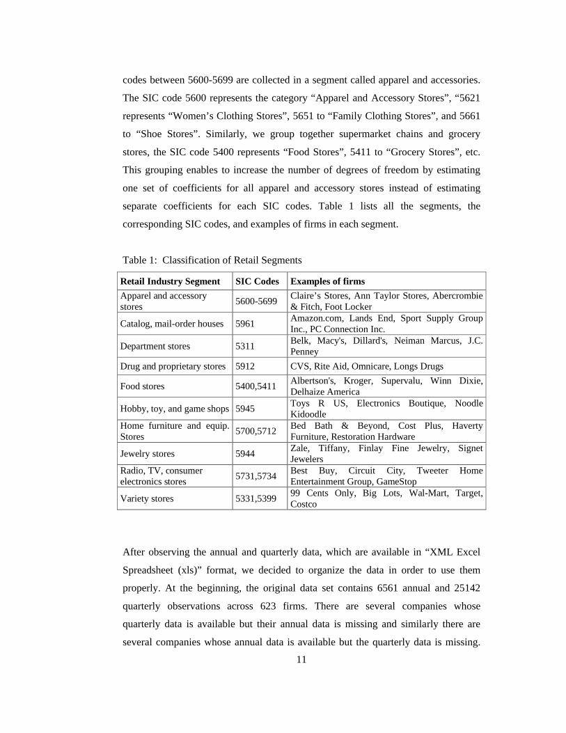
separate coefficients for each SIC codes. Table 1 lists all the segments, the
corresponding SIC codes, and examples of firms in each segment.
Table 1: Classification of Retail Segments
Retail Industry Segment SIC Codes Examples of firms
Apparel and accessory stores
5600-5699Claire’s Stores, Ann Taylor Stores, Abercrombie & Fitch, Foot Locker
Catalog, mail-order houses 5961Amazon.com, Lands End, Sport Supply Group Inc., PC Connection Inc.
Department stores 5311Belk, Macy's, Dillard's, Neiman Marcus, J.C. Penney
Drug and proprietary stores 5912 CVS, Rite Aid, Omnicare, Longs Drugs
Food stores 5400,5411Albertson's, Kroger, Supervalu, Winn Dixie, Delhaize America
Hobby, toy, and game shops 5945Toys R US, Electronics Boutique, Noodle Kidoodle
Home furniture and equip. Stores
5700,5712Bed Bath & Beyond, Cost Plus, Haverty Furniture, Restoration Hardware
Jewelry stores 5944Zale, Tiffany, Finlay Fine Jewelry, Signet Jewelers
Radio, TV, consumer electronics stores
5731,5734Best Buy, Circuit City, Tweeter Home Entertainment Group, GameStop
Variety stores 5331,539999 Cents Only, Big Lots, Wal-Mart, Target, Costco
After observing the annual and quarterly data, which are available in “XML Excel
Spreadsheet (xls)” format, we decided to organize the data in order to use them
properly. At the beginning, the original data set contains 6561 annual and 25142
quarterly observations across 623 firms. There are several companies whose
quarterly data is available but their annual data is missing and similarly there are
several companies whose annual data is available but the quarterly data is missing.

12
Since our study needs both annul and quarterly data and we want to obtain realistic
and sensible results, we eliminated the firms that have neither annual nor quarterly
data set.
While organizing the quarterly data set, we follow several steps in Microsoft Visual
Basic. Primarily, there are 4 fiscal quarters per year. In the quarter data, both the
fiscal quarters and the corresponding fiscal years are available. Normally, it is
expected that a fiscal year starts with fiscal quarter “1”, and it follows as “2”, “3” and
ends with fiscal quarter “4”. However, there are some years that do not obey this
rule. What we do is, check whether each firm’s available fiscal quarters of the years
follow this rule or not. If not, delete the data corresponding to these years. Then, we
exclude the firms that had missing data other than at the beginning or the end of their
fiscal years. If the firms had missing data at the beginning or end of the measurement
period, delete just the related years. The reason for these missing data might be
bankruptcy filings, and subsequent emergence from bankruptcy. Further, for any sub-
period during 1985-2003, we omit from our data set the firms that have less than
seven consecutive years of data available for more accurate results. After completing
the elimination process in the quarterly data, we revise the annual data accordingly.
After organizing the data set as above, it is observed that the numbers of annual
observations are 4236; quarterly observations are 16944 across 304 firms. Following
this, we compute the performance variables. The computation of sales forecasts,
using Holt’s and Winter’s Method, require at least two years of sales data at the
beginning of each time series. Therefore, the first two years data could not be used in
the analysis and we omit the first two years of data of each firm.
Our final data set contains 3628 annual, 14512 quarterly observations across 304
firms, and an average of 11.93 years of data per firm. Gaur et al. (2005) use financial
data for publicly listed U.S. retailers for the 16-year period 1985-2000. Although our
study consider the 25-year period 1985-2009, the number of firms that are observed
are less in our case. Their final data set contains 3407 annual observations across 311
firms.
13
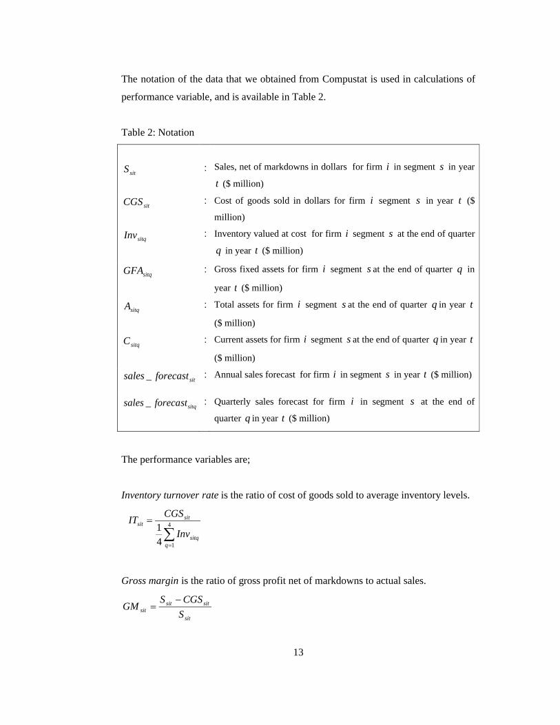
The notation of the data that we obtained from Compustat is used in calculations of
performance variable, and is available in Table 2.
Table 2: Notation
The performance variables are;
Inventory turnover rate is the ratio of cost of goods sold to average inventory levels.
4
14
1
qsitq
sitsit
Inv
CGSIT
Gross margin is the ratio of gross profit net of markdowns to actual sales.
sit
sitsitsit S
CGSSGM
sitS : Sales, net of markdowns in dollars for firm i in segment s in year
t ($ million)
sitCGS : Cost of goods sold in dollars for firm i segment s in year t ($
million)
sitqInv : Inventory valued at cost for firm i segment s at the end of quarter
q in year t ($ million)
sitqGFA : Gross fixed assets for firm i segment s at the end of quarter q in
year t ($ million)
sitqA : Total assets for firm i segment s at the end of quarter q in year t
($ million)
sitqC : Current assets for firm i segment s at the end of quarter q in year t
($ million)
sitforecastsales _ : Annual sales forecast for firm i in segment s in year t ($ million)
sitqforecastsales _ : Quarterly sales forecast for firm i in segment s at the end of
quarter q in year t ($ million)

14
Capital intensity is the ratio of average fixed assets to average total assets.
4
1
4
1
4
1
qsitq
qsitq
qsitq
sit
GFAInv
GFA
CI
Gross fixed assets, sitqGFA = sitqsitq CA
Sales surprise is the ratio of actual sales to expected sales for the year.
sit
sitsit forecastsales
SSS
_
Mean Absolute Percentage Error (quarterly) is a measure of accuracy in a fitted
timed series
100_
sitq
sitqsitq
qsit S
forecastsalesSMAPE
Mean Absolute Percentage Error (annual),
4
14
1
qsitqsit MAPEMAPE
The annual sales forecasts are estimated using Holt’s double exponential smoothing
method which allows for simultaneous smoothing on the time series and the linear
trend. The method requires the specification of smoothing constants and . It uses
two smoothing equations: one for the value of the series (the intercept) and one for
the trend (the slope) respectively. We use the formulations of Holt’s method given by
Nahmias (2005) with the notations that are provided below. Table 3 lists the
definition of the parameters used in Holt’s method.

15
Table 3: Notation for Holt’s Method
))(1( 1,1, tsitsisitsit TGSG
1,1, )1()( tsitsisitsit TGGT , where (0 < < 1) and (0 < < 1) .
The 1-step-ahead forecast made in period t-1, which is denoted by sitforecastsales _
is given by
1,1,_ tsitsisit TGforecastsales
Initialization Procedure for Holt’s Method
In order to get the method started, we have to have initial estimates for the slope and
the intercept.
sitsit Sforecastsales _
sitsit SG
sittsisit SST 1,
The quarterly sales forecast are estimated using Winter’s triple exponential
smoothing method and has the advantage of being easy to update new data becomes
available. The length of the season is N periods, and the method requires the
specification of smoothing constants , and .
In our study, as there are 4 quarters in each year, the length of the season is 4 periods
(N=4). We use the formulations of Winter’s method given by Nahmias (2005) with
the notations that are provided below. Table 4 lists the definition of the parameters
used in Winter’s method.
sitG : Value of the intercept for firm i in segment s in year t ($ million)
sitT : Value of the slope for firm i in segment s in year t ($ million)
: Smoothing constant for the intercept
: Smoothing constant for the slope
16
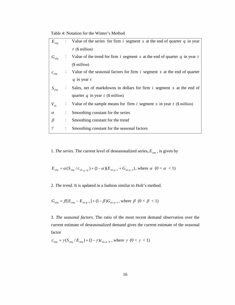
Table 4: Notation for the Winter’s Method
1. The series. The current level of deseasonalized series, sitqE , is given by
))(1()/( 1,1,, qsitqsitNqsitsitqsitq GEcSE , where (0 < < 1)
2. The trend. It is updated in a fashion similar to Holt’s method.
1,1, )1(][ qsitqsitsitqsitq GEEG , where (0 < < 1)
3. The seasonal factors. The ratio of the most recent demand observation over the
current estimate of deseasonalized demand gives the current estimate of the seasonal
factor
Nqsitsitqsitqsitq cESc ,)1()/( , where (0 < < 1)
sitqE : Value of the series for firm i segment s at the end of quarter q in year
t ($ million)
sitqG : Value of the trend for firm i segment s at the end of quarter q in year t
($ million)
sitqc : Value of the seasonal factors for firm i segment s at the end of quarter
q in year t
sitqS : Sales, net of markdowns in dollars for firm i segment s at the end of
quarter q in year t ($ million)
sitV : Value of the sample means for firm i segment s in year t ($ million)
: Smoothing constant for the series
: Smoothing constant for the trend
: Smoothing constant for the seasonal factors
17
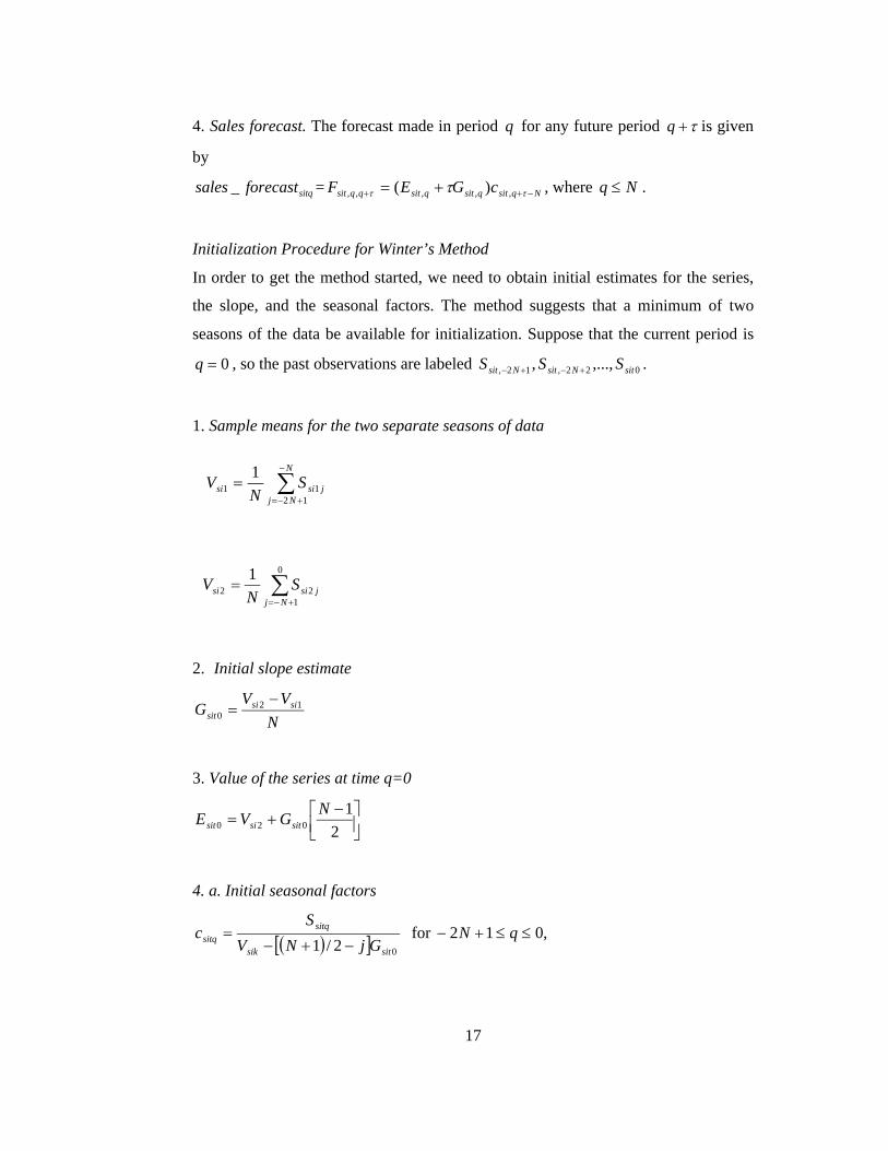
4. Sales forecast. The forecast made in period q for any future period q is given
by
sitqforecastsales _ = Nqsitqsitqsitqqsit cGEF ,,,,, )( , where Nq .
Initialization Procedure for Winter’s Method
In order to get the method started, we need to obtain initial estimates for the series,
the slope, and the seasonal factors. The method suggests that a minimum of two
seasons of the data be available for initialization. Suppose that the current period is
0q , so the past observations are labeled 022,12, ,...,, sitNsitNsit SSS .
1. Sample means for the two separate seasons of data
0
122
1
Njjsisi S
NV
2. Initial slope estimate
N
VVG sisi
sit12
0
3. Value of the series at time q=0
2
1020
NGVE sitsisit
4. a. Initial seasonal factors
02/1 sitsik
sitqsitq GjNV
Sc
for ,012 qN
N
Njjsisi S
NV
1211
1

18
where 1k for the first season(year), 2k for the second season(year), and j is the
period(quarter) of the season(year). That is, 1j for 12 Nq and 1 Nq ;
2j for 22 Nq and 2 Nq , and so on.
b. Average seasonal forecasts assuming that exactly two seasons of initial data
2,...,
20,
01,12,
1,sitNsit
sitNsitNsit
Nsit
ccc
ccc
c. Normalize the seasonal factors
Nc
cc
N
ksikj
sitjsitj .
1
0
for 01 jN
Here, using quarterly closing values, average inventory, average gross fixed assets,
quarterly sales forecast are computed so as to control for systematic seasonal changes
in these variables during the year. The method for obtaining the annual sales forecast
and quarterly sales forecast will be described in Chapter 4.
Table 5 shows the descriptive statistics for each retailing segment for the
performance variables by listing the mean, median and standard deviation. For the
variety stores, for instance, the average inventory turnover rate for variety is 4.154,
the standard deviation (stated in parenthesis) is 2.398 and the median inventory rate
is 3.448. It is detected that food retailers have the lowest mean gross margin of 0.25
and the highest mean inventory turnover of 11.38. On the contrary, jewelry stores
have the highest mean gross margin of 0.41 and the lowest mean inventory turns of
2.32.

19
Retail Industry Segment
SIC codesNumber of firms
Number of annual observations
Average annual sales($ million)
Average inventory turnover
Average gross margin
Average capital intensity
Average sales surprise
Average mean abs. perc. error
Median Inventory Turnover
Median Gross Margin
Median Capital Intensity
Median Sales Surprise
Median mean abs. perc. error
Apparel and accessory stores 5600-5699 73 935 1,536.658 4.111 0.362 0.240 1.015
0.0653.942 0.357 0.224 1.001 0.048
(1.691) (0.099) (0.116) (0.282) (0.06)Catalog, mail-order houses 5961 39 380 830.261 8.741 0.360 0.288 1.077
0.1285.612 0.371 0.225 0.225 0.07
(7.828) (0.154) (0.213) (0.555) (0.109)
Department stores 5311 21 289 4,775.720 3.222 0.334 0.268 1.058 0.055 3.141 0.348 0.275 1.005 0.037(0.816) (0.074) (0.087) (0.375) (0.046)
Drug and proprietary stores 5912 23 267 6,593.223 9.574 0.261 0.286 1.21
0.0745.367 0.275 0.223 1.017 0.04
(12.305) (0.079) (0.223) (1.33) (0.145)
Food stores 5400,5411 54 674 6,896.458 11.379 0.252 0.420 1.022 0.107 10.423 0.262 0.421 0.999 0.03(4.487) (0.078) (0.128) (0.201) (1.349)
Hobby, toy, and game shops 5945 7 80 3,117.592 2.652 0.322 0.171 0.930
0.0962.429 0.343 0.146 1.003 0.047
(0.905) (0.096) (0.103) (0.555) (0.16)Home furniture and equip. stores 5700,5712 19 232 846.137 3.942 0.395 0.229 1.02
0.0642.979 0.405 0.195 1.008 0.048
(5.132) (0.085) (0.132) (0.16) (0.05)
Jewelry stores 5944 14 163 691.170 2.323 0.411 0.125 1.027 0.121 1.340 0.470 0.110 0.999 0.072(4.303) (0.144) (0.068) (0.242) (0.19)
Radio, TV,consumer electronics stores 5731,5734 17 201 3,586.531 3.776 0.317 0.155 1.028 0.079 3.659 0.289 0.139 1.014 0.054
(1.382) (0.103) (0.082) (0.200) (0.08)
Variety stores 5331,5399 37 407 14,669.962 4.154 0.285 0.196 1.013 0.056 3.448 0.279 0.171 1.008 0.039(2.398) (0.084) (0.114) (0.188) (0.06)
Table 5: Summary statistics of the variables for each segment
20
Chapter 4
HYPOTHESIS DEVELOPMENT
In this chapter, we set up hypotheses to relate inventory turnover to gross margin,
capital intensity, sales surprise and mean absolute percentage error in seasonal sales
forecast using data for 304 publicly listed U.S. retailers for the period 1985-2009.
Gaur et al. (2005) study the correlation of inventory turnover with gross margin,
capital intensity and sales surprise for the period 1985-2000. In their paper, gross
margin, capital intensity, and sales surprise are defined as shown in the previous
chapter. In this study, we study the impact of quarterly sales forecast inaccuracy, as
measured with mean absolute percentage error, on inventory turnover ratio.
4.1. Gross Margin
Hypothesis 1. Inventory turnover is negatively correlated with gross margin.
Gross margin is the proportion of gross profit net of markdowns (difference between
actual sales and the production costs excluding taxation, interest payments, payroll)
to actual sales. It represents the percentage of total sales revenue that the firm retains

21
after incurring the direct costs. The higher the gross margin has, the more efficient
company is. Retailers would be inclined to carry more inventory for products with
higher gross margins as they would want to reduce or eliminate the number of stock-
outs. Gaur et al. (2005) test this hypothesis using the data from period 1985-2009.
Using larger and more recent data set, we would like to detect consistency and
compare the current results to them.
4.1. Capital Intensity
Hypothesis 2. Inventory turnover is positively correlated with capital intensity.
Capital intensity specifies how much money is invested to produce one dollar of
sales revenue. Therefore, retailers with high capital intensity mean investing more on
information technology, machinery, management systems, etc. which increase their
efficiency in operations. The companies can follow and meet the customers’
demands easily and it is easy to increase their productivity and customer satisfaction
which affects the inventory turnover positively. Again, this hypothesis is tested in
Gaur et al. (2005) and we would like to retest it with a larger and more current
dataset.
4.2. Sales Surprise
Hypothesis 3. Inventory turnover is positively correlated with sales surprise.
Sales surprise is ratio of actual sales to sales forecast. Sales surprise will increase if
the demand is underestimated which means that actual sales are higher than the sales
forecast. Since the actual sales are more in quantity, the average inventory level
decreases which would lead to a one time increase in the inventory turnover ratio for
that year. Alternatively, if the sales surprise is small, we would have a one time
reduction increase in the inventory turnover for that year as there would be an
inventory build-up.
22
We follow Gaur et al. (2005) and use Holt’s method to calculate sales forecasts. In
Holt’s method, and values need to optimized for best forecast accuracy. The
forecast errors for several values of and are compared by Gaur et al. (2005),
and it is observed that 75.0 and 75.0 give the best forecasts. Although we
do not have completely same data set, we use the same smoothing constant values in
our analysis.
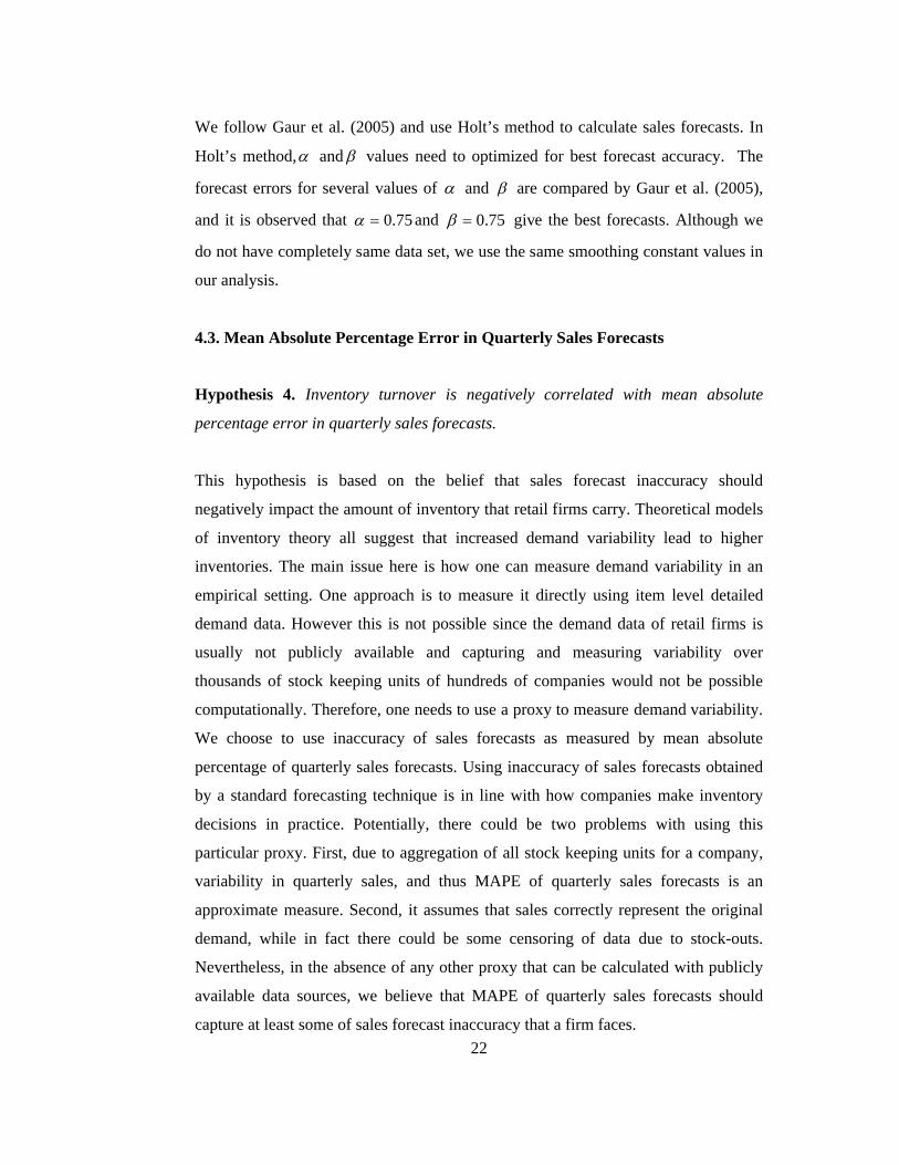
4.3. Mean Absolute Percentage Error in Quarterly Sales Forecasts
Hypothesis 4. Inventory turnover is negatively correlated with mean absolute
percentage error in quarterly sales forecasts.
This hypothesis is based on the belief that sales forecast inaccuracy should
negatively impact the amount of inventory that retail firms carry. Theoretical models
of inventory theory all suggest that increased demand variability lead to higher
inventories. The main issue here is how one can measure demand variability in an
empirical setting. One approach is to measure it directly using item level detailed
demand data. However this is not possible since the demand data of retail firms is
usually not publicly available and capturing and measuring variability over
thousands of stock keeping units of hundreds of companies would not be possible
computationally. Therefore, one needs to use a proxy to measure demand variability.
We choose to use inaccuracy of sales forecasts as measured by mean absolute
percentage of quarterly sales forecasts. Using inaccuracy of sales forecasts obtained
by a standard forecasting technique is in line with how companies make inventory
decisions in practice. Potentially, there could be two problems with using this
particular proxy. First, due to aggregation of all stock keeping units for a company,
variability in quarterly sales, and thus MAPE of quarterly sales forecasts is an
approximate measure. Second, it assumes that sales correctly represent the original
demand, while in fact there could be some censoring of data due to stock-outs.
Nevertheless, in the absence of any other proxy that can be calculated with publicly
available data sources, we believe that MAPE of quarterly sales forecasts should
capture at least some of sales forecast inaccuracy that a firm faces.
23
Since quarterly sales forecast data includes seasonality, as stated in Chapter 3, we
estimate sales forecasts from available data using Winter’s triple exponential
smoothing method. We compared the forecast errors for 125 different values of
, and . All combinations of 0.1, 0.3, 0.5, 0.7, 0.9, for , and are observed
((0.1,0.1,0.1), (0.1,0.1,0.3), (0.1,0.1,0.5),…(0.9,0.9,0.9)) so that we have to run the
macro code 125 times. In order to decide the best , and pair for our models, we
try several approaches.
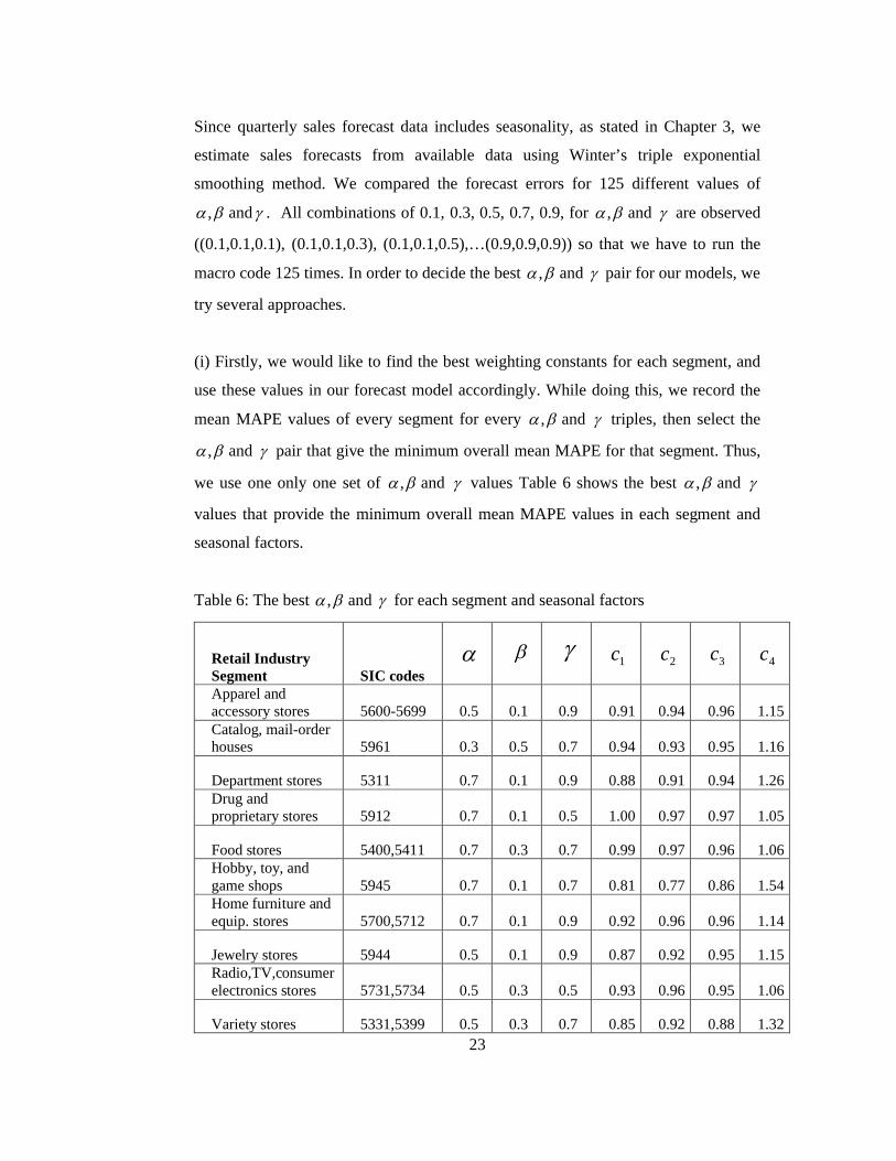
(i) Firstly, we would like to find the best weighting constants for each segment, and
use these values in our forecast model accordingly. While doing this, we record the
mean MAPE values of every segment for every , and triples, then select the
, and pair that give the minimum overall mean MAPE for that segment. Thus,
we use one only one set of , and values Table 6 shows the best , and
values that provide the minimum overall mean MAPE values in each segment and
seasonal factors.
Table 6: The best , and for each segment and seasonal factors
Retail Industry Segment SIC codes
1c 2c 3c 4c
Apparel and accessory stores 5600-5699 0.5 0.1 0.9 0.91 0.94 0.96 1.15Catalog, mail-order houses 5961 0.3 0.5 0.7 0.94 0.93 0.95 1.16
Department stores 5311 0.7 0.1 0.9 0.88 0.91 0.94 1.26Drug and proprietary stores 5912 0.7 0.1 0.5 1.00 0.97 0.97 1.05
Food stores 5400,5411 0.7 0.3 0.7 0.99 0.97 0.96 1.06Hobby, toy, and game shops 5945 0.7 0.1 0.7 0.81 0.77 0.86 1.54Home furniture and equip. stores 5700,5712 0.7 0.1 0.9 0.92 0.96 0.96 1.14
Jewelry stores 5944 0.5 0.1 0.9 0.87 0.92 0.95 1.15Radio,TV,consumer electronics stores 5731,5734 0.5 0.3 0.5 0.93 0.96 0.95 1.06
Variety stores 5331,5399 0.5 0.3 0.7 0.85 0.92 0.88 1.32
24
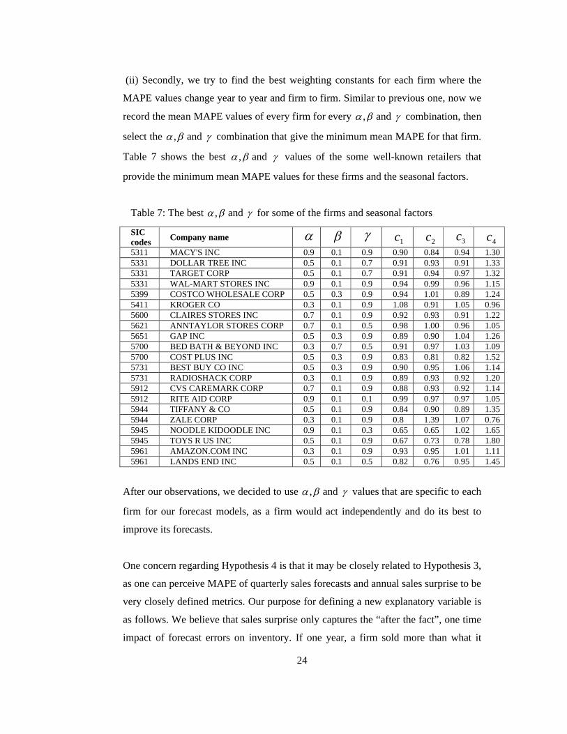
(ii) Secondly, we try to find the best weighting constants for each firm where the
MAPE values change year to year and firm to firm. Similar to previous one, now we
record the mean MAPE values of every firm for every , and combination, then
select the , and combination that give the minimum mean MAPE for that firm.
Table 7 shows the best , and values of the some well-known retailers that
provide the minimum mean MAPE values for these firms and the seasonal factors.
Table 7: The best , and for some of the firms and seasonal factors
SIC codes
Company name 1c 2c 3c 4c
5311 MACY'S INC 0.9 0.1 0.9 0.90 0.84 0.94 1.305331 DOLLAR TREE INC 0.5 0.1 0.7 0.91 0.93 0.91 1.335331 TARGET CORP 0.5 0.1 0.7 0.91 0.94 0.97 1.325331 WAL-MART STORES INC 0.9 0.1 0.9 0.94 0.99 0.96 1.155399 COSTCO WHOLESALE CORP 0.5 0.3 0.9 0.94 1.01 0.89 1.245411 KROGER CO 0.3 0.1 0.9 1.08 0.91 1.05 0.965600 CLAIRES STORES INC 0.7 0.1 0.9 0.92 0.93 0.91 1.225621 ANNTAYLOR STORES CORP 0.7 0.1 0.5 0.98 1.00 0.96 1.055651 GAP INC 0.5 0.3 0.9 0.89 0.90 1.04 1.265700 BED BATH & BEYOND INC 0.3 0.7 0.5 0.91 0.97 1.03 1.095700 COST PLUS INC 0.5 0.3 0.9 0.83 0.81 0.82 1.525731 BEST BUY CO INC 0.5 0.3 0.9 0.90 0.95 1.06 1.145731 RADIOSHACK CORP 0.3 0.1 0.9 0.89 0.93 0.92 1.205912 CVS CAREMARK CORP 0.7 0.1 0.9 0.88 0.93 0.92 1.145912 RITE AID CORP 0.9 0.1 0.1 0.99 0.97 0.97 1.055944 TIFFANY & CO 0.5 0.1 0.9 0.84 0.90 0.89 1.355944 ZALE CORP 0.3 0.1 0.9 0.8 1.39 1.07 0.765945 NOODLE KIDOODLE INC 0.9 0.1 0.3 0.65 0.65 1.02 1.655945 TOYS R US INC 0.5 0.1 0.9 0.67 0.73 0.78 1.805961 AMAZON.COM INC 0.3 0.1 0.9 0.93 0.95 1.01 1.115961 LANDS END INC 0.5 0.1 0.5 0.82 0.76 0.95 1.45
After our observations, we decided to use , and values that are specific to each
firm for our forecast models, as a firm would act independently and do its best to
improve its forecasts.
One concern regarding Hypothesis 4 is that it may be closely related to Hypothesis 3,
as one can perceive MAPE of quarterly sales forecasts and annual sales surprise to be
very closely defined metrics. Our purpose for defining a new explanatory variable is
as follows. We believe that sales surprise only captures the “after the fact”, one time
impact of forecast errors on inventory. If one year, a firm sold more than what it

25
projected, its inventory would be less than what it would projected. Alternatively, if
the firm sold less than what it projected, its inventory would be more than it would
be projected. With MAPE of quarterly forecasts, we would like to measure the
impact of demand variability on a firm’s decisions. If a firm knows that it is exposed
to high forecast inaccuracy (or high demand variability), it would stock more safety
stock to maintain its service level (which is assumed to be high in retail).
Alternatively, if the firm’s forecasts are usually accurate, it would not plan for too
much stock.
Despite these arguments, however, we still need to understand the correlation
between these two metrics as both are based on actual and forecasted values of
demand. Table 8 shows the correlation coefficients’ estimates and the statistics for
different segments. At 0.01 level, there is significant correlation between these two
metrics only for the drug and propriety stores (positive correlation) and variety stores
(negative correlation).
Table 8: Pearson Correlation of Sales Surprise and Mean Absolute Percentage Error
Retail Industry Segment SIC Codes Estimate P-value
Apparel and accessory stores 5600-5699 -0,003 0,918
Catalog, mail-order houses 5961 0,086 0,095
Department stores 5311 0,1 0,09
Drug and proprietary stores 5912 0,161 0,008
Food stores 5400,5411 0,03 0,443
Hobby, toy, and game shops 5945 -0,273 0,015
Home furniture and equip. stores 5700,5712 -0,027 0,681
Jewelry stores 5944 -0,142 0,07
Radio,TV, consumer electronics stores 5731,5734 -0,077 0,277
Variety stores 5331,5399 -0,129 0,009

26
Chapter 5
EMPIRICAL MODEL
We propose 5 models to test our hypotheses so as to draw further insights and better
estimation than in Gaur et al. (2005). In each of the 5 models, we use different sets of
explanatory variables, different combination of parameters, like gross margin, sitGM ,
capital intensity, sitCI , sales surprise, sitSS , and mean absolute percentage error,
sitMAPE . The results of these different combinations of parameters and models, are
compared in Chapter 6.
Until we finalize our data set, we try several data sets to observe different scenarios.
We estimate the sub models with values of (1) only mean absolute percentage error
lagged by one year (2) gross margin, capital intensity, sales surprise and mean
absolute percentage error lagged by one year, (3) mean absolute percentage error
values obtained by the scenario (i) in Chapter 4, (4) mean absolute percentage error
values obtained by the scenario (ii) in Chapter 4.
27
The final data set that we use is (4), in which mean absolute percentage error values
are obtained by the scenario (ii) and are not lagged.
We now provide the regression models that we use in our study.
Models
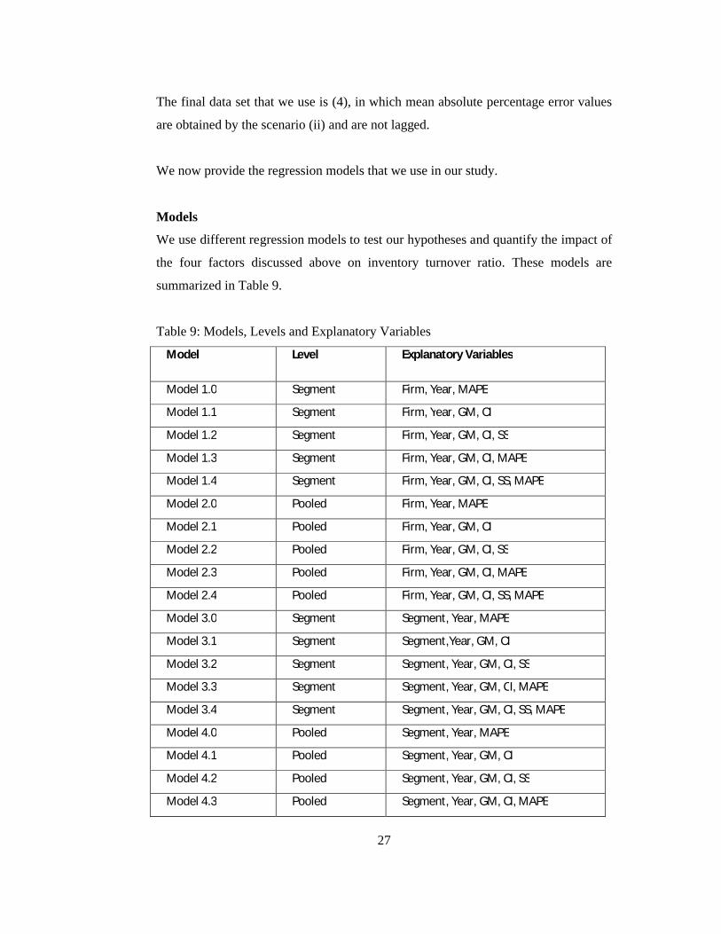
We use different regression models to test our hypotheses and quantify the impact of
the four factors discussed above on inventory turnover ratio. These models are
summarized in Table 9.
Table 9: Models, Levels and Explanatory Variables
Model Level Explanatory Variables
Model 1.0 Segment Firm, Year, MAPE
Model 1.1 Segment Firm, Year, GM, CI
Model 1.2 Segment Firm, Year, GM, CI, SS
Model 1.3 Segment Firm, Year, GM, CI, MAPE
Model 1.4 Segment Firm, Year, GM, CI, SS, MAPE
Model 2.0 Pooled Firm, Year, MAPE
Model 2.1 Pooled Firm, Year, GM, CI
Model 2.2 Pooled Firm, Year, GM, CI, SS
Model 2.3 Pooled Firm, Year, GM, CI, MAPE
Model 2.4 Pooled Firm, Year, GM, CI, SS, MAPE
Model 3.0 Segment Segment, Year, MAPE
Model 3.1 Segment Segment,Year, GM, CI
Model 3.2 Segment Segment, Year, GM, CI, SS
Model 3.3 Segment Segment, Year, GM, CI, MAPE
Model 3.4 Segment Segment, Year, GM, CI, SS, MAPE
Model 4.0 Pooled Segment, Year, MAPE
Model 4.1 Pooled Segment, Year, GM, CI
Model 4.2 Pooled Segment, Year, GM, CI, SS
Model 4.3 Pooled Segment, Year, GM, CI, MAPE

28
Model 4.4 Pooled Segment, Year, GM, CI, SS, MAPE
Model 5.0 Pooled Year, MAPE
Model 5.1 Pooled Year, GM, CI
Model 5.2 Pooled Year, GM, CI, SS
Model 5.3 Pooled Year, GM, CI, MAPE
Model 5.4 Pooled Year, GM, CI, SS, MAPE
Model 1 uses firm and time specific fixed effects because we desire to control the
impacts of these to our regression model. For each segment, regression models are
run separately as the coefficients of estimates depend on segments.
Model 2 again use firm and time specific fixed effects; however, regression analysis
is not carried out separately for each segment and segment specific coefficient
estimates are not used. Now, the coefficients of estimate of a variable, GM for
instance, are same for all the segments. Consequently, the coefficient of estimation
for GM, CI, SS, and MAPE do not depend on the segments.
Model 3 uses segment and time specific fixed effects, and similar to Model 1,
segment specific coefficient estimates are used. With the help of this model, we can
compare the significance of firm specific effects with segment specific effects.
Similar to Model 3, Model 4 uses segment and time specific fixed effects;
nevertheless, segment specific coefficient estimates are not used, as Model 2. Pooled
coefficients of the variables GM, CI, SS, and MAPE are used as a replacement for
segmentwise coefficients. We test whether coefficients of the variables change across
segments.
To control for the fixed effects, Model 5 includes just time specific fixed effects.
Like Model 2 and Model 4, we do not carry out regression analysis separately for
each segment; as a result, segment specific coefficient estimates are not used. The
definition of the variables and the coefficients used in these 5 models are available in
Table 10.

29
5.1. Model 1
In this model, we control the effects of time (year) and firms in each segment while
estimating how GM, CI, SS, and MAPE influence a firm’s IT. Hence, it is better to
use tc as a time-specific fixed effect, iF as a firm-specific fixed effects.
We would like to observe the effects of sales surprise and mean absolute percentage
error to our models; therefore, (1.1) includes neither sales surprise nor mean absolute
percentage error. Equation (1.1) just examines GM’s and CI’s effects on IT. In the
Models (1.2) and (1.3), SS and MAPE are put into models respectively to compare
their effects. In Model (1.1), both SS and MAPE variables are considered together.
The results of Models (1.1)-(1.2) and (1.1)-(1.3) are compared at first. Then, (1.2)-
(1.4) and (1.3)-(1.4) are evaluated respectively in Chapter 6.
Not only in Models (1.1), (1.2), (1.3), (1.4) but also in the other Models (2.1),
(2.2),…, (5.4), we expect that 0, 11 bbs and 0, 22 bbs , 0, 33 bbs , 0, 44 bbs owing
to the hypotheses that we state in Chapter 4.
Table 10: Notation for the regression models
iF : Time-invariant firm-specific fixed effect for firm i
sF : Time-invariant segment-specific fixed effect for segment s
tc : Year-specific fixed effect for year t
1sb : coefficient of sitGMln for segment s
2sb : coefficient of sitCIln for segment s
3sb : coefficient of sitSSln for segment s
4sb : coefficient of sitMAPEln for segment s
1b : coefficient of sitGMln
2b : coefficient of sitCIln
30
3b : coefficient of sitSSln
4b : coefficient of sitMAPEln
sit : error term for segment s , firm i , year t
sitsitstisit MAPEbcFIT lnln 4 (1.0)
sitsitssitstisit CIbGMbcFIT lnlnln 21 (1.1)
sitsitssitssitstisit SSbCIbGMbcFIT lnlnlnln 321 (1.2)
sitsitssitssitstisit MAPEbCIbGMbcFIT lnlnlnln 421 (1.3)
sitsitssitssitssitstisit MAPEbSSbCIbGMbcFIT lnlnlnlnln 4321 (1.4)
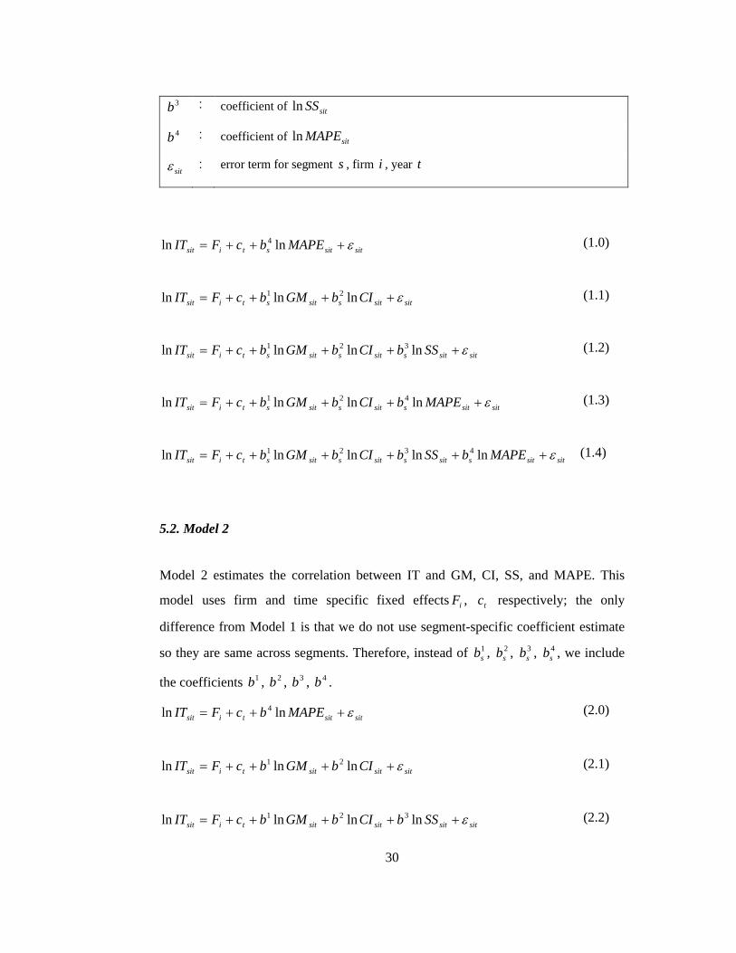
5.2. Model 2
Model 2 estimates the correlation between IT and GM, CI, SS, and MAPE. This
model uses firm and time specific fixed effects iF , tc respectively; the only
difference from Model 1 is that we do not use segment-specific coefficient estimate
so they are same across segments. Therefore, instead of 1sb , 2
sb , 3sb , 4
sb , we include
the coefficients 1b , 2b , 3b , 4b .
sitsittisit MAPEbcFIT lnln 4 (2.0)
sitsitsittisit CIbGMbcFIT lnlnln 21 (2.1)
sitsitsitsittisit SSbCIbGMbcFIT lnlnlnln 321 (2.2)

31
sitsitsitsittisit MAPEbCIbGMbcFIT lnlnlnln 421 (2.3)
sitsitsitsitsittisit MAPEbSSbCIbGMbcFIT lnlnlnlnln 4321 (2.4)
5.3. Model 3
Model 3 uses segment specific fixed effects sF , time specific fixed effects tc and
segment specific coefficient estimates 1sb , 2
sb , 3sb , 4
sb .
sitsitstssit MAPEbcFIT lnln 4 (3.0)
sitsitssitstssit CIbGMbcFIT lnlnln 21 (3.1)
sitsitssitssitstssit SSbCIbGMbcFIT lnlnlnln 321 (3.2)
sitsitssitssitstssit MAPEbCIbGMbcFIT lnlnlnln 421 (3.3)
sitsitssitssitssitstssit MAPEbSSbCIbGMbcFIT lnlnlnlnln 4321 (3.4)
5.4. Model 4
Model 4 uses segment specific fixed effects sF , time specific fixed effects tc and
similar to Model 2, pooled coefficients estimates 1b , 2b , 3b , 4b .
sitsittssit MAPEbcFIT lnln 4 (4.0)
sitsitsittssit CIbGMbcFIT lnlnln 21 (4.1)

32
sitsitsitsittssit SSbCIbGMbcFIT lnlnlnln 321 (4.2)
sitsitsitsittssit MAPEbCIbGMbcFIT lnlnlnln 421 (4.3)
sitsitsitsitsittssit MAPEbSSbCIbGMbcFIT lnlnlnlnln 4321 (4.4)
5.5 Model 5
Here, time specific fixed effects tc , and pooled coefficients estimates 1b , 2b , 3b , 4b
(similar to Model 2 and 4) are considered.
sitsittsit MAPEbcIT lnln 4 (5.0)
sitsitsittsit CIbGMbcIT lnlnln 21 (5.1)
sitsitsitsittsit SSbCIbGMbcIT lnlnlnln 321 (5.2)
sitsitsitsittsit MAPEbCIbGMbcIT lnlnlnln 421 (5.3)
sitsitsitsitsittsit MAPEbSSbCIbGMbcIT lnlnlnlnln 4321 (5.4)

33
Chapter 6
NUMERICAL RESULTS
We begin with the analysis of correlation between merely inventory turnover rate
and mean absolute percentage error. Before observing the different combinations of
explanatory variables, we look at the effect of mean absolute percentage error on
inventory turnover rate in each of the 5 models. Model 1.0, Model 2.0, Model 3.0,
Model 4.0 and Model 5.0 are the sub-models that are used to test the hypotheses.
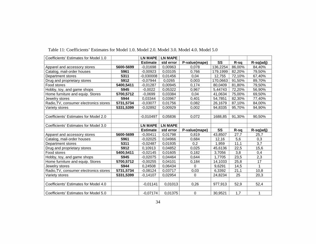
Table 11 shows the coefficients’ estimates and statistics of the sub-models that are
mentioned above. It is observed that in most of the case, inventory turnover is
negatively correlated with mean absolute percentage error in quarterly sales forecast.
The other 4 versions of Model 1 are denoted as Model 1.1, Model 1.2, Model 1.3,
and Model 1.4. In Model 1.1, the effects of gross margin and capital intensity on
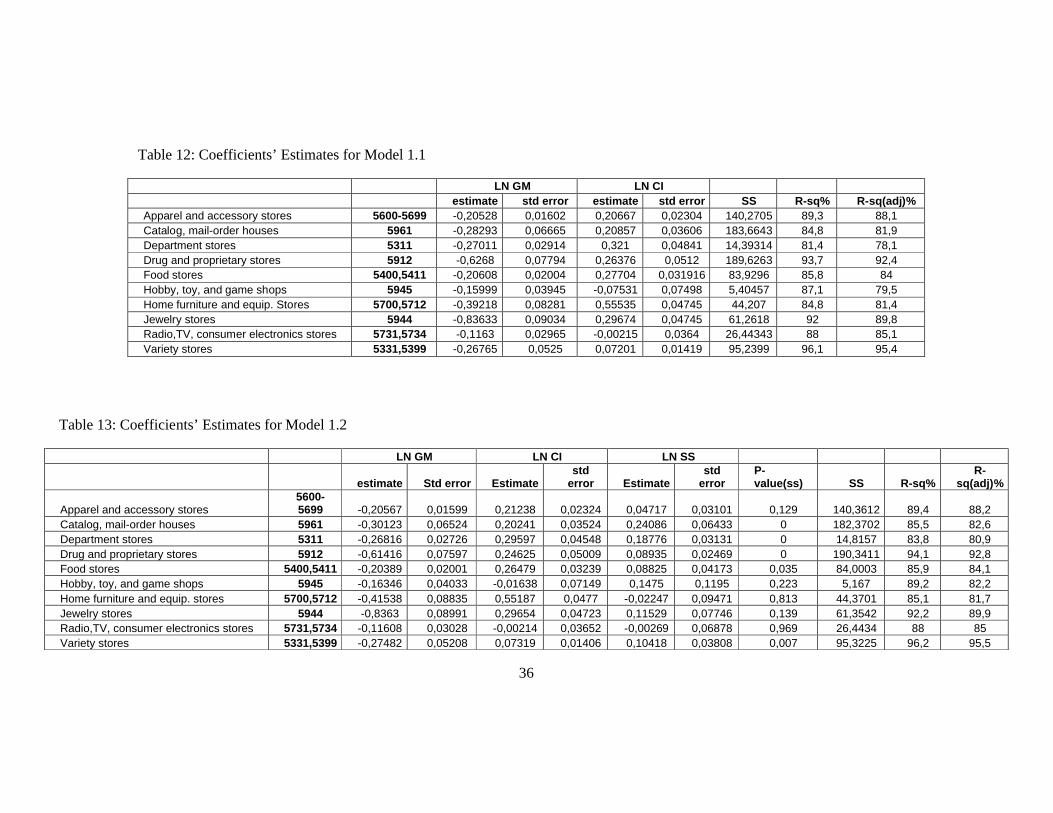
inventory turnover ratio are observed. Table 12 shows the coefficients’ estimates and
statistics of the Model 1.1. It is realized that in all segments, the coefficients
estimates of gross margin are negative, 01 sb . Except two segments, with SIC codes
5945 and 5731, 5734 “Hobby, toy, and game shops” and “Radio, TV, consumer
34
Coefficients' Estimates for Model 1.0 LN MAPE LN MAPEEstimate std error P-value(mape) SS R-sq R-sq(adj)
Apparel and accessory stores 5600-5699 -0,01698 0,00963 0,078 136,2254 86,00% 84,40%Catalog, mail-order houses 5961 -0,00923 0,03105 0,766 179,1999 82,20% 79,50%Department stores 5311 -0,030008 0,01456 0,04 12,755 72,10% 67,40%Drug and proprietary stores 5912 -0,07944 0,0265 0,003 170,0663 91,50% 89,70%Food stores 5400,5411 -0,01287 0,00945 0,174 80,0409 81,80% 79,50%Hobby, toy, and game shops 5945 -0,0022 0,05322 0,967 5,44743 72,20% 56,90%Home furniture and equip. Stores 5700,5712 -0,0699 0,03384 0,04 41,0634 75,00% 69,50%Jewelry stores 5944 0,03344 0,03967 0,401 54,7851 82,30% 77,40%Radio,TV, consumer electronics stores 5731,5734 -0,03077 0,01756 0,082 26,1679 87,10% 84,00%Variety stores 5331,5399 -0,02892 0,00929 0,002 94,8335 95,70% 94,90%
Coefficients' Estimates for Model 2.0 -0,010497 0,05836 0,072 1688,85 91,30% 90,50%
Coefficients' Estimates for Model 3.0 LN MAPE LN MAPEEstimate std error P-value(mape) SS R-sq R-sq(adj)
Apparel and accessory stores 5600-5699 -0,00411 0,01798 0,819 43,8507 27,7 25,7Catalog, mail-order houses 5961 -0,02025 0,04966 0,684 12,16 5,6 0,3Department stores 5311 -0,02487 0,01935 0,2 1,959 11,1 3,7Drug and proprietary stores 5912 0,10913 0,04852 0,025 45,6136 22,5 15,6Food stores 5400,5411 -0,02145 0,01605 0,182 3,7056 3,8 0,4Hobby, toy, and game shops 5945 -0,02075 0,04464 0,644 1,7705 23,5 2,3Home furniture and equip. Stores 5700,5712 -0,00255 0,04101 0,184 14,1033 25,8 17Jewelry stores 5944 0,24508 0,06434 0 9,6291 14,5 1Radio,TV, consumer electronics stores 5731,5734 -0,08124 0,03717 0,03 6,3392 21,1 10,8Variety stores 5331,5399 -0,14107 0,02954 0 24,8234 25 20,3
Coefficients' Estimates for Model 4.0 -0,01141 0,01013 0,26 977,913 52,9 52,4
Coefficients' Estimates for Model 5.0 -0,07174 0,01375 0 30,9521 1,7 1
Table 11: Coefficients’ Estimates for Model 1.0, Model 2.0, Model 3.0, Model 4.0, Model 5.0
35
electronic stores” respectively, coefficients estimates of capital intensity are
positive 02 sb .
These results support Hypotheses 1 and 2. A %1 increase in gross margin leads to
decrease in gross margin in all segments; however, the amount of this decrease varies
across segment.
Table 13 shows the results of Model 1.2, where the performance variable sales
surprise is added to regression model. Again, we observe the negative correlation
between gross margin and inventory turnover in all segments; positive correlation
between capital intensity and inventory turnover; positive correlation between sales
surprise and inventory turnover for eight of the ten segments. Comparing the
Adjusted R-Square values of Models 1.1 and 1.2, we detect that for nine of the ten
segments, these values increase, which is expected. The highest increase in Adjusted
R-Square value (R-sq(adj)) is recognized in the “Hobby, toy, and game shops”
segment. The reason for comparing these two sub models in terms of their Adjusted
R-Square values is that it is generally considered to be an accurate goodness-of-fit
measure.
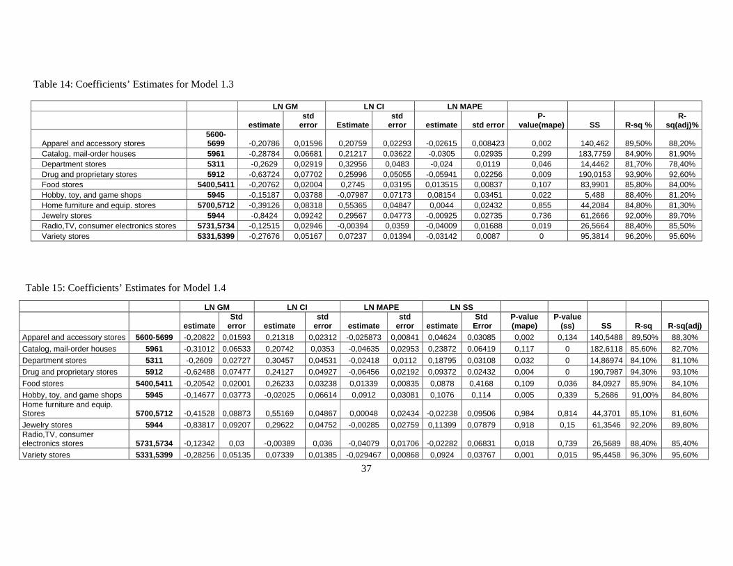
We include the performance variable, mean absolute percentage error, instead of
sales surprise in the Model 1.3. The coefficients’ of the gross margin and capital
intensity are consistent with the previous models. Moreover, segmentwise estimates
of the coefficient of sitMAPEln supports the Hypothesis 4, 03 sb , for seven of the
ten segments. The detailed coefficients’ estimates are available in Table 14. When
we compare the R-sq(adj) values of (1.1) and (1.3), we observe that the values
remain same in “Catalog-mail order houses” and “food stores” segments; slight
decrease in “Jewelry stores” and “Home furniture and equipment stores”. On the
other hand, for six of the ten segments, increase in R-sq(adj) value is noticed. Once
more, highest increase in R-sq(adj) is recognized in the “Hobby, toy, and game
shops” segment.
36
LN GM LN CIestimate std error estimate std error SS R-sq% R-sq(adj)%
Apparel and accessory stores 5600-5699 -0,20528 0,01602 0,20667 0,02304 140,2705 89,3 88,1Catalog, mail-order houses 5961 -0,28293 0,06665 0,20857 0,03606 183,6643 84,8 81,9Department stores 5311 -0,27011 0,02914 0,321 0,04841 14,39314 81,4 78,1Drug and proprietary stores 5912 -0,6268 0,07794 0,26376 0,0512 189,6263 93,7 92,4Food stores 5400,5411 -0,20608 0,02004 0,27704 0,031916 83,9296 85,8 84Hobby, toy, and game shops 5945 -0,15999 0,03945 -0,07531 0,07498 5,40457 87,1 79,5Home furniture and equip. Stores 5700,5712 -0,39218 0,08281 0,55535 0,04745 44,207 84,8 81,4Jewelry stores 5944 -0,83633 0,09034 0,29674 0,04745 61,2618 92 89,8Radio,TV, consumer electronics stores 5731,5734 -0,1163 0,02965 -0,00215 0,0364 26,44343 88 85,1Variety stores 5331,5399 -0,26765 0,0525 0,07201 0,01419 95,2399 96,1 95,4
LN GM LN CI LN SS
estimate Std error Estimate std
error Estimatestd
errorP-value(ss) SS R-sq%
R-sq(adj)%
Apparel and accessory stores5600-5699 -0,20567 0,01599 0,21238 0,02324 0,04717 0,03101 0,129 140,3612 89,4 88,2
Catalog, mail-order houses 5961 -0,30123 0,06524 0,20241 0,03524 0,24086 0,06433 0 182,3702 85,5 82,6Department stores 5311 -0,26816 0,02726 0,29597 0,04548 0,18776 0,03131 0 14,8157 83,8 80,9Drug and proprietary stores 5912 -0,61416 0,07597 0,24625 0,05009 0,08935 0,02469 0 190,3411 94,1 92,8Food stores 5400,5411 -0,20389 0,02001 0,26479 0,03239 0,08825 0,04173 0,035 84,0003 85,9 84,1Hobby, toy, and game shops 5945 -0,16346 0,04033 -0,01638 0,07149 0,1475 0,1195 0,223 5,167 89,2 82,2Home furniture and equip. stores 5700,5712 -0,41538 0,08835 0,55187 0,0477 -0,02247 0,09471 0,813 44,3701 85,1 81,7Jewelry stores 5944 -0,8363 0,08991 0,29654 0,04723 0,11529 0,07746 0,139 61,3542 92,2 89,9Radio,TV, consumer electronics stores 5731,5734 -0,11608 0,03028 -0,00214 0,03652 -0,00269 0,06878 0,969 26,4434 88 85Variety stores 5331,5399 -0,27482 0,05208 0,07319 0,01406 0,10418 0,03808 0,007 95,3225 96,2 95,5
Table 12: Coefficients’ Estimates for Model 1.1
Table 13: Coefficients’ Estimates for Model 1.2
37
:
LN GM LN CI LN MAPE LN SS
estimateStd
error estimate std
error estimatestd
error estimateStd
ErrorP-value(mape)
P-value(ss) SS R-sq R-sq(adj)
Apparel and accessory stores 5600-5699 -0,20822 0,01593 0,21318 0,02312 -0,025873 0,00841 0,04624 0,03085 0,002 0,134 140,5488 89,50% 88,30%
Catalog, mail-order houses 5961 -0,31012 0,06533 0,20742 0,0353 -0,04635 0,02953 0,23872 0,06419 0,117 0 182,6118 85,60% 82,70%
Department stores 5311 -0,2609 0,02727 0,30457 0,04531 -0,02418 0,0112 0,18795 0,03108 0,032 0 14,86974 84,10% 81,10%
Drug and proprietary stores 5912 -0,62488 0,07477 0,24127 0,04927 -0,06456 0,02192 0,09372 0,02432 0,004 0 190,7987 94,30% 93,10%
Food stores 5400,5411 -0,20542 0,02001 0,26233 0,03238 0,01339 0,00835 0,0878 0,4168 0,109 0,036 84,0927 85,90% 84,10%
Hobby, toy, and game shops 5945 -0,14677 0,03773 -0,02025 0,06614 0,0912 0,03081 0,1076 0,114 0,005 0,339 5,2686 91,00% 84,80%Home furniture and equip. Stores 5700,5712 -0,41528 0,08873 0,55169 0,04867 0,00048 0,02434 -0,02238 0,09506 0,984 0,814 44,3701 85,10% 81,60%
Jewelry stores 5944 -0,83817 0,09207 0,29622 0,04752 -0,00285 0,02759 0,11399 0,07879 0,918 0,15 61,3546 92,20% 89,80%Radio,TV, consumer electronics stores 5731,5734 -0,12342 0,03 -0,00389 0,036 -0,04079 0,01706 -0,02282 0,06831 0,018 0,739 26,5689 88,40% 85,40%
Variety stores 5331,5399 -0,28256 0,05135 0,07339 0,01385 -0,029467 0,00868 0,0924 0,03767 0,001 0,015 95,4458 96,30% 95,60%
LN GM LN CI LN MAPE
estimatestd
error Estimate std
error estimate std errorP-
value(mape) SS R-sq %R-
sq(adj)%
Apparel and accessory stores5600-5699 -0,20786 0,01596 0,20759 0,02293 -0,02615 0,008423 0,002 140,462 89,50% 88,20%
Catalog, mail-order houses 5961 -0,28784 0,06681 0,21217 0,03622 -0,0305 0,02935 0,299 183,7759 84,90% 81,90%Department stores 5311 -0,2629 0,02919 0,32956 0,0483 -0,024 0,0119 0,046 14,4462 81,70% 78,40%Drug and proprietary stores 5912 -0,63724 0,07702 0,25996 0,05055 -0,05941 0,02256 0,009 190,0153 93,90% 92,60%Food stores 5400,5411 -0,20762 0,02004 0,2745 0,03195 0,013515 0,00837 0,107 83,9901 85,80% 84,00%Hobby, toy, and game shops 5945 -0,15187 0,03788 -0,07987 0,07173 0,08154 0,03451 0,022 5,488 88,40% 81,20%Home furniture and equip. stores 5700,5712 -0,39126 0,08318 0,55365 0,04847 0,0044 0,02432 0,855 44,2084 84,80% 81,30%Jewelry stores 5944 -0,8424 0,09242 0,29567 0,04773 -0,00925 0,02735 0,736 61,2666 92,00% 89,70%Radio,TV, consumer electronics stores 5731,5734 -0,12515 0,02946 -0,00394 0,0359 -0,04009 0,01688 0,019 26,5664 88,40% 85,50%Variety stores 5331,5399 -0,27676 0,05167 0,07237 0,01394 -0,03142 0,0087 0 95,3814 96,20% 95,60%
Table 14: Coefficients’ Estimates for Model 1.3
Table 15: Coefficients’ Estimates for Model 1.4

38
In addition to gross margin and capital intensity, Model 1.4 includes the performance
variables sales surprise and mean absolute percentage error. All the coefficients’
estimates support the Hypotheses 1, 2, 3 and 4 where 01 sb and 02 sb , 03 sb ,
04 sb . Table 15 lists the detailed statistics of Model 1.4. Except “Home furniture
and equipment stores” segment, all the R-sq(adj) values are both higher in Model 1.4
and Model 1.3 than Model 1.2. Greatest improvement in R-sq(adj) is recognized in
the “Hobby, toy, and game shops” segment.
Instead of segment-specific coefficients, pooled coefficients are used in Model 2 to
test the hypotheses. There are 4 other versions of this model in which we perform
different combinations of the parameters, sitGM , sitCI , sitSS , sitMAPE as Model 1.
The overall fit of Models 2.1, 2.2, 2.3, and 2.4 are statistically significant. Table 16
shows the coefficients’ estimates for Model 2.1. Here, as we state in the previous
chapter, the coefficients of estimation do not vary segment to segment. The pooled
coefficients for sitGMln is -0.26653, sitCIln is 0.23001, and strongly support
Hypothesis 1 and Hypothesis 2 respectively.
Model 2.2 supports the Hypotheses 1, 2 and 3. We observe that Adjusted R-Square
value in Model 2.2 is higher compared to Model 2.1. For eight of the ten segments,
R-Sq(adj) value in Model 2.2 is greater than R-Sq(adj) values in Model 1.2. Table 17
shows the statistics for Model 2.2.
Model 2.3 supports the Hypotheses 1, 2 and 4. We observe that Adjusted R-Square
value in Model 2.3 is same as Model 2.1. Furthermore, Model 2.3 is not as
statistically significant as Model 2.2. Table 18 shows the statistics for Model 2.3.
The pooled coefficients for sitGMln , sitCIln , sitSSln , sitMAPEln in Model 2.4 prove
that all hypotheses are supported. Adjusted R-Square value in Model 2.4 is higher
compared to Model 2.1, 2.2 and 2.3. Except two segments, “Drug and proprietary
stores” and “Variety stores”, R-Sq(adj) value in Model 2.4 is greater than R-Sq(adj)
values in Model 1.4. The statistics for Model 2.4 are available in Table 19.

39
LN GM LN CI
estimateStd
error Estimate Std
error SS R-sq% R-sq(adj)%-0,26653 0,0119 0,23001 0,01088 1718,866 93,2 92,6
Table 17: Coefficients’ Estimates for Model 2.2
LN GM LN CI LN SS
estimateStd
error Estimate Std
error Estimatestd
errorP-value(ss) SS R-sq%
R-sq(adj)%
-0,26664 0,0118 0,22818 0,01079 0,10845 0,01353 0 1714,802 93,4 92,7
Table 18: Coefficients’ Estimates for Model 2.3
LN GM LN CI LN MAPE
Estimatestd
error estimate Std
error Estimatestd
errorP-
value(mape) SS R-sq %R-
sq(adj)%-0,26732 0,1678 0,23115 0,01087 -0,01593 0,00516 0,002 1719,226 93,30% 92,60%
Table 19: Coefficients’ Estimates for Model 2.4
LN GM LN CI LN MAPE LN SS
Estimatestd
error Estimate Std
error Estimatestd
error estimatestd
errorP-value(mape)
P-value(ss) SS R-sq
R-sq(adj)
-0,2675 0,01179 0,2293 0,01078 -0,01666 0,00511 0,10786 0,01351 0,001 0 1715,193 93,40% 92,80%
Table 16: Coefficients’ Estimates for Model 2.1
40
To compare the significance of firm-specific fixed effects with segmentwise fixed
effect, Model 3 is developed. Similar to the first two models, there are 4 other
versions of Model 3. This model is functional and provides better estimation than
Model 1, since it contains fewer parameters. Tables 20, 21, 22 and 23 show the
statistics for Models 3.1, 3.2, 3.3 and 3.4 respectively. All the hypotheses stated in
Chapter 4 are supported significantly by these models.
From Model 3.1, it is realized that in all segments, the coefficients estimates of gross
margin are negative, 01 sb and coefficients estimates of capital intensity are
positive 02 sb , which are similar results with Model 1.1. One primary difference
between two Models is that 3.1 gives more precise estimation, hence segment-
specific fixed effects are statistically significant.
For Model 3.2, the segmentwise estimates of the coefficient of sitGMln , sitCIln ,
sitSSln support Hypotheses 1, 2 and 3. R-Sq(adj) values in Model 3.2 is greater than
R-Sq(adj) values in Model 3.1. After comparing Models 3.2 and 3.1, we detect that
greatest improvements in R-sq(adj) are recognized in the “Department stores”
segments.
The R-Sq(adj) values in Model 3.3 is better than both in Model 3.1 and 3.2 so we
can state that mean absolute percentage error is a better determinant of inventory
turnover ratio than sales surprise. Comparing Models 3.3 and 3.1, we detect that
greatest improvements in R-sq(adj) are recognized in the “Home furniture and
equipment stores” segments.
The Model 3.4 includes all the performance variables in a single model. Majority of
coefficients’ estimates support the Hypotheses 1, 2, 3 and 4 where 01 sb and
02 sb , 03 sb , 04 sb .

41
LN GM LN CI
estimate std error estimate std error SS R-sq% R-sq(adj)%
Apparel and accessory stores 5600-5699 -0,33828 0,02418 0,42252 0,02057 85,0174 54,1 52,8
Catalog, mail-order houses 5961 -0,92767 0,04897 0,38078 0,03106 122,5417 56,6 53,8
Department stores 5311 -0,23953 0,03547 0,21942 0,0303 6,67982 37,8 32,4
Drug and proprietary stores 5912 -0,97683 0,07499 0,52488 0,04081 152,712 75,5 73,1
Food stores 5400,5411 -0,27067 0,02856 0,44865 0,03961 24,6429 25,2 22,4
Hobby, toy, and game shops 5945 -0,29864 0,0557 0,1332 0,04323 3,09766 49,9 29
Home furniture and equip. Stores 5700,5712 -0,7058 0,1195 0,46785 0,05934 18,6956 35,9 28
Jewelry stores 5944 -1,02336 0,05794 0,41576 0,05531 51,5386 77,4 73,7
Radio,TV, consumer electronics stores 5731,5734 -0,38833 0,04928 0,17543 0,05185 12,79006 42,5 34,7
Variety stores 5331,5399 -1,02621 0,03806 0,27281 0,01795 80,8728 81,6 80,4
Table 21: Coefficients’ Estimates for Model 3.2
LN GM LN CI LN SS
Estimate Std error estimate std
error estimatestd
errorP-value(ss) SS
R-sq%
R-sq(adj)%
Apparel and accessory stores 5600-5699 -0,33824 0,02409 0,42688 0,02056 0,02782 0,05991 0,129 85,7215 54,6 53,2Catalog, mail-order houses 5961 -0,93809 0,04781 0,37393 0,03041 0,30622 0,09501 0,001 124,8305 58,5 55,7Department stores 5311 -0,23243 0,03497 0,21911 0,02981 0,17551 0,05614 0 7,07261 40 34,5Drug and proprietary stores 5912 -0,96325 0,07401 0,51845 0,04026 0,13012 0,04467 0 154,3935 76,3 73,9Food stores 5400,5411 -0,27152 0,02857 0,45204 0,03975 -0,08945 0,08809 0,035 24,7592 25,3 22,4Hobby, toy, and game shops 5945 -0,31607 0,05569 0,13213 0,04224 0,3642 0,2142 0,095 3,00693 51,9 29,7Home furniture and equip. Stores 5700,5712 -0,7546 0,1251 0,48378 0,06048 0,2405 0,1815 0,813 19,0796 36,6 28,5Jewelry stores 5944 -1,01705 0,05763 0,40603 0,05518 0,214 0,1224 0,139 51,8642 77,9 74,1Radio,TV, consumer electronics stores 5731,5734 -0,39553 0,04932 0,1745 0,05166 0,2081 0,1361 0,969 13,01774 43,3 35,2Variety stores 5331,5399 -1,02428 0,03785 0,27236 0,01785 0,1759 0,07504 0,007 81,1336 81,9 80,6
Table 20: Coefficients’ Estimates for Model 3.1

42
LN GM LN GM LN CI LN CI LN MAPE LN MAPE LN SS LN SS
estimateStderror
estimate std
errorestimate
stderror
estimatestderror
P-value(mape)
P-value(ss)
SS R-sq% R-sq(adj)%
Apparel and accessory stores5600-5699
-0,33917 0,02421 0,42658 0,02058 -0,0059 0,01443 0,02813 0,05994 0,683 0,639 85,7347 54,6 53,2
Catalog, mail-order houses 5961 -0,94879 0,04725 0,37667 0,02999 -0,11315 0,03405 0,33818 0,09417 0,001 0 127,5251 59,8 56,9Department stores 5311 -0,24435 0,0346 0,22095 0,02932 -0,05019 0,01593 0,19637 0,05561 0,002 0 7,45877 42,2 36,7Drug and proprietary stores 5912 -1,01193 0,07171 0,50523 0,03854 -0,03766 0,02666 0,05463 0,07655 0,159 0,476 145,8107 78,4 76,3Food stores 5400,5411 -0,273 0,0285 0,45591 0,03967 -0,03063 0,01414 -0,08443 0,08787 0,031 0,337 25,2852 25,8 22,9Hobby, toy, and game shops 5945 -0,25369 0,06017 0,17253 0,04434 0,10328 0,04536 0,2269 0,2147 0,027 0,296 3,26368 56,4 35Home furniture and equip. Stores
5700,5712 -0,7739 0,1178 0,52463 0,05639 0,19853 0,03412 0,2411 0,2067 0 0,245 25,5085 49,4 42,6
Jewelry stores 5944 -0,97911 0,06508 0,42261 0,05666 0,04693 0,03768 0,2351 0,1234 0,215 0,059 52,0288 78,2 74,2Radio, TV, consumer electronics stores
5731,5734 -0,40108 0,04825 0,18258 0,05056 -0,09466 0,0313 0,1567 0,1341 0,003 0,244 13,8686 46,1 38,1
Variety stores 5331,5399 -1,01002 0,03759 0,26658 0,0177 -0,04918 0,01473 0,14626 0,07458 0,001 0,051 81,6488 82,4 81,1
LN GM LN CI LN MAPE
Estimatestd
error estimate std
error estimatestd
errorP-value(mape) SS R-sq % R-sq(adj)%
Apparel and accessory stores 5600-5699 -0,33897 0,0243 0,42228 0,0206 -0,00441 0,01448 0,761 85,0248 54,1 52,8
Catalog, mail-order houses 5961 -0,93293 0,04886 0,38356 0,03099 -0,06154 0,03368 0,068 123,4174 57 54,1
Department stores 5311 -0,25059 0,0355 0,22104 0,02995 -0,0435 0,01615 0,008 6,97406 39,4 33,9
Drug and proprietary stores 5912 -1,0176 0,0712 0,50474 0,03849 -0,03427 0,0262 0,192 145.7241 78,4 76,2
Food stores 5400,5411 -0,27221 0,02848 0,45275 0,03954 -0,03099 0,01414 0,029 25,1816 25,7 22,9
Hobby, toy, and game shops 5945 -0,26558 0,05848 0,15718 0,04504 0,06703 0,04098 0,108 3,24434 52,3 31,1
Home furniture and equip. Stores 5700,5712 -0,7472 0,1157 0,51913 0,05624 0,20172 0,03404 0 25,3301 49,1 42,4
Jewelry stores 5944 -0,99389 0,06523 0,42961 0,05708 0,03707 0,03768 0,327 51,6433 77,6 73,7
Radio,TV, consumer electronics stores 5731,5734 -0,39602 0,0481 0,18366 0,05061 -0,09929 0,03108 0,002 13,7415 45,7 38
Variety stores 5331,5399 -1,0106 0,03773 0,26655 0,01776 -0,05262 0,01468 0 81,4711 82,2 81
Table 22: Coefficients’ Estimates for Model 3.3
Table 23: Coefficients’ Estimates for Model 3.4
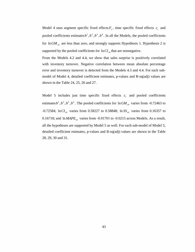
43
Model 4 uses segment specific fixed effects sF , time specific fixed effects tc and
pooled coefficients estimates 1b , 2b , 3b , 4b . In all the Models, the pooled coefficients
for sitGMln are less than zero, and strongly supports Hypothesis 1. Hypothesis 2 is
supported by the pooled coefficients for sitCIln that are nonnegative.
From the Models 4.2 and 4.4, we show that sales surprise is positively correlated
with inventory turnover. Negative correlation between mean absolute percentage
error and inventory turnover is detected from the Models 4.3 and 4.4. For each sub-
model of Model 4, detailed coefficient estimates, p-values and R-sq(adj) values are
shown in the Table 24, 25, 26 and 27.
Model 5 includes just time specific fixed effects tc and pooled coefficients
estimates 1b , 2b , 3b , 4b . The pooled coefficients for sitGMln varies from -0.72463 to
-0.72584; sitCIln varies from 0.58227 to 0.58848; sitSSln varies from 0.16357 to
0.16718; and sitMAPEln varies from -0.01701 to -0.0215 across Models. As a result,
all the hypotheses are supported by Model 5 as well. For each sub-model of Model 5,
detailed coefficient estimates, p-values and R-sq(adj) values are shown in the Table
28, 29, 30 and 31.
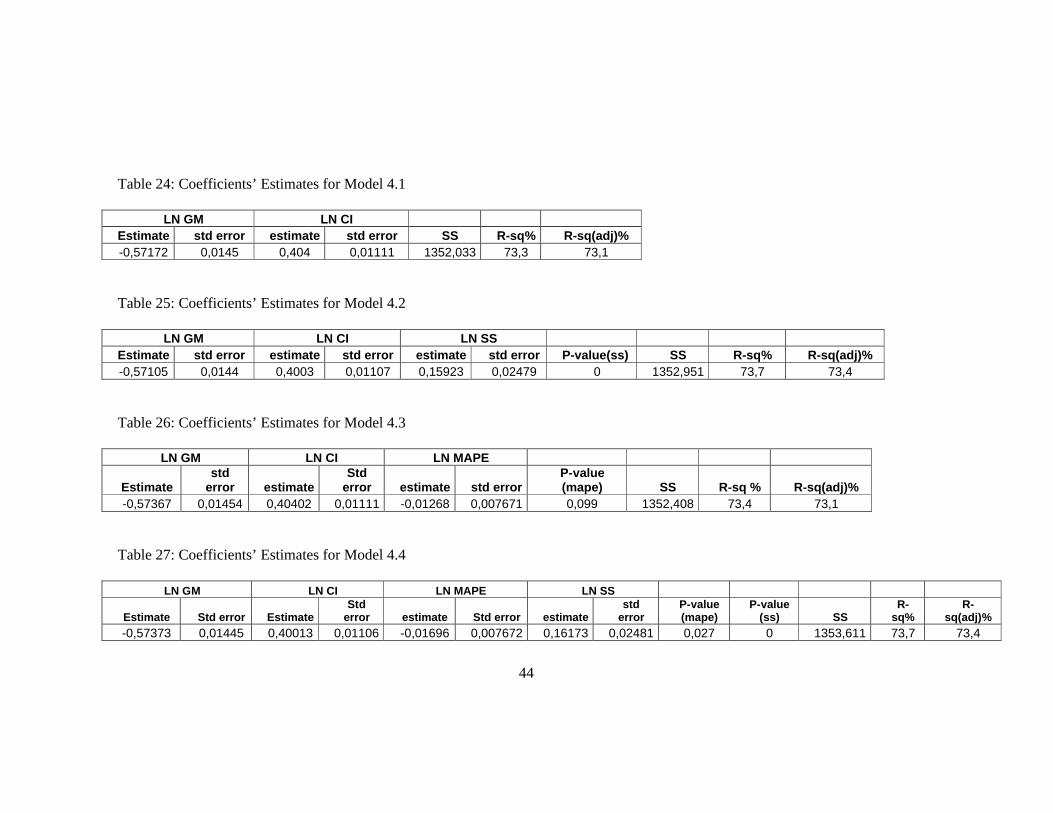
44
Table 24: Coefficients’ Estimates for Model 4.1
LN GM LN CIEstimate std error estimate std error SS R-sq% R-sq(adj)%-0,57172 0,0145 0,404 0,01111 1352,033 73,3 73,1
Table 25: Coefficients’ Estimates for Model 4.2
LN GM LN CI LN SSEstimate std error estimate std error estimate std error P-value(ss) SS R-sq% R-sq(adj)%-0,57105 0,0144 0,4003 0,01107 0,15923 0,02479 0 1352,951 73,7 73,4
Table 26: Coefficients’ Estimates for Model 4.3
LN GM LN CI LN MAPE
Estimatestd
error estimate Std
error estimate std errorP-value(mape) SS R-sq % R-sq(adj)%
-0,57367 0,01454 0,40402 0,01111 -0,01268 0,007671 0,099 1352,408 73,4 73,1
Table 27: Coefficients’ Estimates for Model 4.4
LN GM LN CI LN MAPE LN SS
Estimate Std error Estimate Std
error estimate Std error estimatestd
errorP-value(mape)
P-value(ss) SS
R-sq%
R-sq(adj)%
-0,57373 0,01445 0,40013 0,01106 -0,01696 0,007672 0,16173 0,02481 0,027 0 1353,611 73,7 73,4
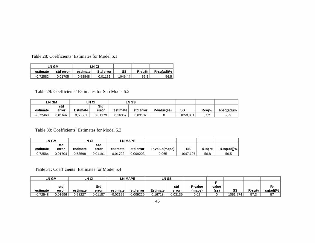
45
LN GM LN CI
estimate std error estimate Std error SS R-sq% R-sq(adj)%
-0,72582 0,01705 0,58848 0,01183 1046,44 56,8 56,5
Table 29: Coefficients’ Estimates for Sub Model 5.2
LN GM LN CI LN SS
estimatestd
error Estimate Std
error estimate std error P-value(ss) SS R-sq% R-sq(adj)%
-0,72463 0,01697 0,58561 0,01179 0,16357 0,03137 0 1050,081 57,2 56,9
Table 30: Coefficients’ Estimates for Model 5.3
LN GM LN CI LN MAPE
estimatestd
error estimate Std
error estimate std error P-value(mape) SS R-sq % R-sq(adj)%
-0,72584 0,01704 0,58598 0,01191 -0,01702 0,009203 0,065 1047,197 56,8 56,5
LN GM LN CI LN MAPE LN SS
estimatestd
error estimate Std
error estimate std error Estimatestd
errorP-value(mape)
P-value(ss) SS R-sq%
R-sq(adj)%
-0,72548 0,01696 0,58227 0,01187 -0,02155 0,009229 0,16718 0,03139 0,02 0 1051,274 57,3 57
Table 28: Coefficients’ Estimates for Model 5.1
Table 31: Coefficients’ Estimates for Model 5.4

46
After finding the coefficients of estimations for each sub problem, we decide to
calculate ~
ln sitIT to observe the variation from sitITln . The firm, whose
~
lnln sitsit ITIT value is above zero, is considered to perform better than the others.
Conversely, if ~
lnln sitsit ITIT value is below zero, the inventory performance of the
firm is below the benchmark.
In order to calculate ~
ln sitIT , we use the coefficient estimates of Model 3.4, i.e.,
sitssitssitssitstssit MAPEbSSbCIbGMbcFIT ln~
ln~
ln~
ln~
ln 4321~
(3.4)
After we calculate ~
lnln sitsit ITIT values for each firm in ten segments, we observe
the distribution of these values by years for all segments, and illustrate them in
Figure 2 through 11. We further present some well-known retailers’ status to give
insight into how well they are operating their inventory systems. It is observed that
the highest ~
lnln sitsit ITIT value is in “Catalog, mail-order houses” segment; the
lowest value is in “Home furniture and equipment stores” segment.
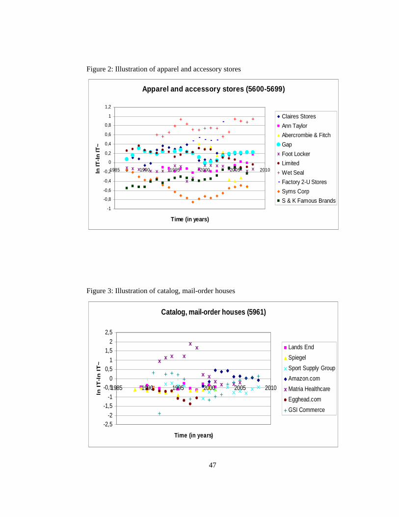
47
Figure 2: Illustration of apparel and accessory stores
Apparel and accessory stores (5600-5699)
-1
-0,8
-0,6
-0,4
-0,2
0
0,2
0,4
0,6
0,8
1
1,2
1985 1990 1995 2000 2005 2010
Time (in years)
ln IT
-ln
IT
~
Claires Stores
Ann Taylor
Abercrombie & Fitch
Gap
Foot Locker
Limited
Wet Seal
Factory 2-U Stores
Syms Corp
S & K Famous Brands
Figure 3: Illustration of catalog, mail-order houses
Catalog, mail-order houses (5961)
-2,5-2
-1,5-1
-0,50
0,51
1,52
2,5
1985 1990 1995 2000 2005 2010
Time (in years)
ln I
T-l
n I
T~
Lands End
Spiegel
Sport Supply Group
Amazon.com
Matria Healthcare
Egghead.com
GSI Commerce
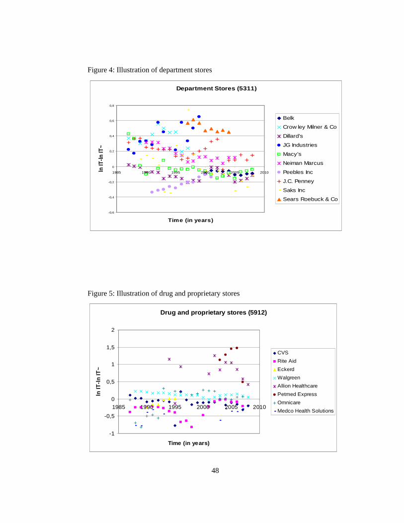
48
Figure 4: Illustration of department stores
Department Stores (5311)
-0,6
-0,4
-0,2
0
0,2
0,4
0,6
0,8
1985 1990 1995 2000 2005 2010
Time (in years)
ln IT
-ln IT
~
Belk
Crow ley Milner & Co
Dillard's
JG Industries
Macy's
Neiman Marcus
Peebles Inc
J.C. Penney
Saks Inc
Sears Roebuck & Co
Figure 5: Illustration of drug and proprietary stores
Drug and proprietary stores (5912)
-1
-0,5
0
0,5
1
1,5
2
1985 1990 1995 2000 2005 2010
Time (in years)
ln IT
-ln
IT~
CVS
Rite Aid
Eckerd
Walgreen
Allion Healthcare
Petmed Express
Omnicare
Medco Health Solutions

49
Figure 6: Illustration of food stores
Food Stores (5400,5411)
-1,5
-1
-0,5
0
0,5
1
1,5
1985 1990 1995 2000 2005 2010
Time (in years)
ln I
T-l
n I
T~
Hannaford Brothers
Kroger
Safeway
Supervalu
Albertsons
General Nutrition
Roundy's
Western Beef
Village Super Market
Figure 7: Illustration of hobby, toy, and game shops
Hobby, toy, and game shops (5945)
-0,8
-0,6
-0,4
-0,2
0
0,2
0,4
0,6
0,8
1985 1990 1995 2000 2005 2010
Time (in years)
ln IT
-ln
IT~
A.C. Moore Arts & Crafts
Electronics Boutique
Lionel
Michaels Stores
Noodle Kidoodle
Rag Shops
Toys R US
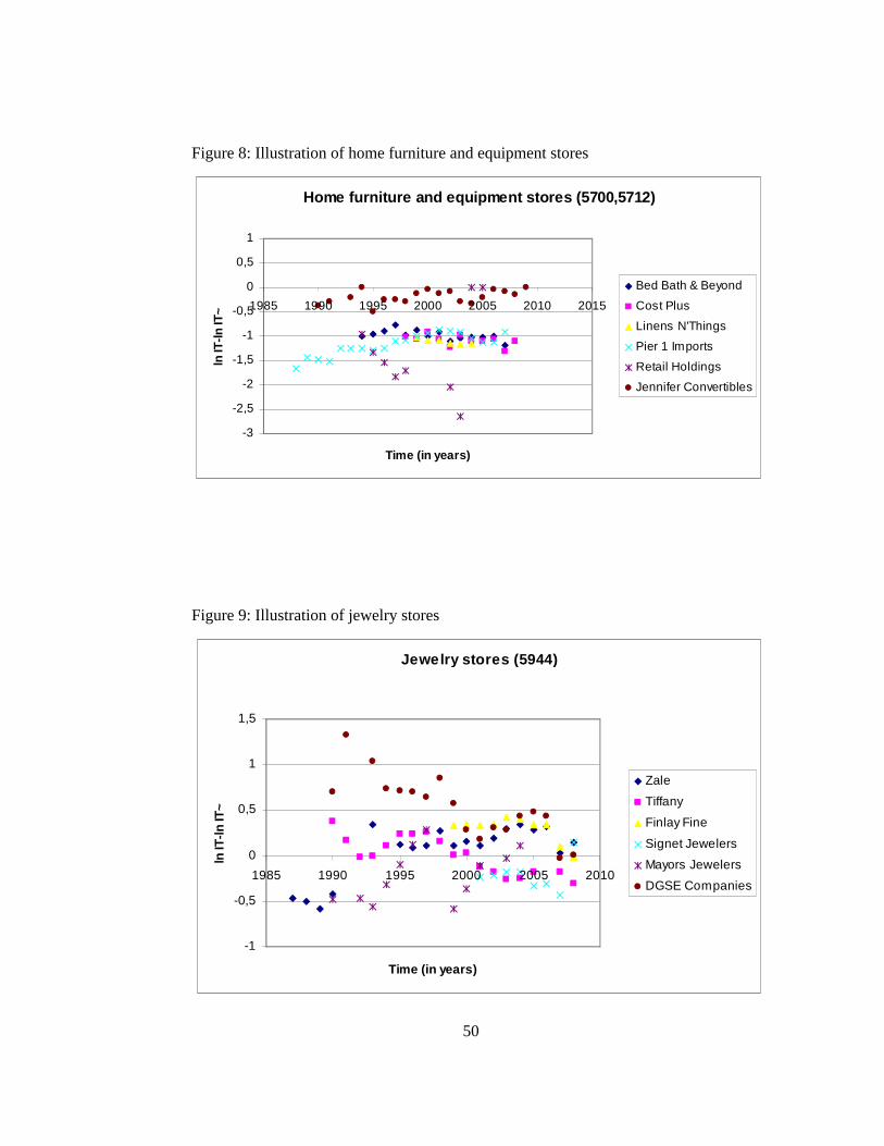
50
Figure 8: Illustration of home furniture and equipment stores
Home furniture and equipment stores (5700,5712)
-3
-2,5
-2
-1,5
-1
-0,5
0
0,5
1
1985 1990 1995 2000 2005 2010 2015
Time (in years)
ln IT
-ln
IT~
Bed Bath & Beyond
Cost Plus
Linens N'Things
Pier 1 Imports
Retail Holdings
Jennifer Convertibles
Figure 9: Illustration of jewelry stores
Jewelry stores (5944)
-1
-0,5
0
0,5
1
1,5
1985 1990 1995 2000 2005 2010
Time (in years)
ln IT
-ln
IT~
Zale
Tiffany
Finlay Fine
Signet Jewelers
Mayors Jewelers
DGSE Companies

51
Figure 10: Illustration of Radio, TV, consumer electronic stores
Radio, TV, consumer electronics stores (5731,5734)
-1,4
-1,2
-1
-0,8
-0,6
-0,4
-0,2
0
0,2
0,4
0,6
1985 1990 1995 2000 2005 2010
Time (in years)
ln IT
-ln
IT~
Best Buy
Circuit City
Good Guys
Harvey Electronics
Intertan
Radioshack
CompUSA
Figure 11: Illustration of variety stores
Variety Stores (5331, 5399)
-1,2
-1
-0,8
-0,6
-0,4
-0,2
0
0,2
0,4
0,6
1985 1990 1995 2000 2005 2010
Time (in years)
ln I
T-l
n I
T~
Wal-Mart
Target
Big Lots
Dollar Tree
Mccrory Corp
99 Cents Only
Sears Holdings Corp
Luria & Son Inc
Service Merchandise Co

52
To sum up, all of our hypotheses are supported by the regression models that are
provided above. We show that mean absolute percentage error in quarterly sales
forecast is negatively correlated with inventory turnover ratio in most of the retail
segments. In order to detect in which segment mean absolute percentage error is
effective, we compare the following models: Model 1.1 to Model 1.3, Model 3.1 to
Model 3.3, Model 1.2 to Model 1.4, and Model 3.2 to Model 3.4.
Model 1.1 vs. Model 1.3: After we add the MAPE as an explanatory variable to the
Model 1.1, we obtain Model 1.3. The largest increase in R-sq (adj) is observed in
“Hobby, toy, and game shops”. Increase in R-sq (adj) is also seen in segments
“Radio, TV, consumer electronics stores”, “Variety stores” and “Department stores”.
Model 3.1 vs. Model 3.3: After we add the MAPE as an explanatory variable to the
Model 3.1, we obtain Model 3.3. The largest increase in R-sq (adj) is observed in
“Home furniture and equipment stores”. Increase in R-sq (adj) is also seen in
segments “Jewelry stores”, “Variety stores” and “Hobby, toy, and game shops”.
Model 1.2 vs. Model 1.4: After we add the MAPE as an explanatory variable to the
Model 1.2, we obtain Model 1.4. The largest increase in R-sq (adj) is again observed
in “Hobby, toy, and game shops”. Hypothesis 4 is strongly supported by the
segments “Radio, TV, consumer electronics stores”, “Variety stores” and
“Department stores”.
Model 3.2 vs. Model 3.4: After we add the MAPE as an explanatory variable to the
Model 3.2, we obtain Model 3.4. The largest increase in R-sq (adj) is observed in
“Hobby, toy, and game shops”. We also detect that hypothesis 4 is supported by the
segments “Home furniture and equipment stores”, “Radio, TV, consumer electronics
stores”, and “Department stores”.
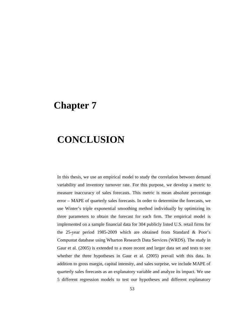
53
Chapter 7
CONCLUSION
In this thesis, we use an empirical model to study the correlation between demand
variability and inventory turnover rate. For this purpose, we develop a metric to
measure inaccuracy of sales forecasts. This metric is mean absolute percentage
error – MAPE of quarterly sales forecasts. In order to deterrmine the forecasts, we
use Winter’s triple exponential smoothing method individually by optimizing its
three parameters to obtain the forecast for each firm. The empirical model is
implemented on a sample financial data for 304 publicly listed U.S. retail firms for
the 25-year period 1985-2009 which are obtained from Standard & Poor’s
Compustat database using Wharton Research Data Services (WRDS). The study in
Gaur et al. (2005) is extended to a more recent and larger data set and tests to see
whether the three hypotheses in Gaur et al. (2005) prevail with this data. In
addition to gross margin, capital intensity, and sales surprise, we include MAPE of
quarterly sales forecasts as an explanatory variable and analyze its impact. We use
5 different regression models to test our hypotheses and different explanatory
54
variables in each of these models to understand the impact of four explanatory
variables on inventory turnover ratio. The first model uses firm and time specific
fixed effects because we desire to control the impacts of these to our regression
model. The second model uses firm and time specific fixed effects as well;
however, regression analysis is not carried out separately for each segment. The
third model uses segment and time specific fixed effects to compare the
significance of firm specific effects with segment specific effects. The fourth
model uses segment and time specific fixed effects; nevertheless, regression
analysis is not carried out separately for each segment. The last model uses just
time specific fixed effects, and we do not carry out regression analysis separately
for each segment.
Some key conclusions and insights drawn from these studies are as follows. We
observe that in most of the sub-segments, except “Hobby, toy, and game shops”,
“Home furniture and equipment stores”, of US retail industry, MAPE is negatively
correlated with inventory turnover ratio. In many sub-segments, introducing MAPE
helps to explain more of the variability of inventory turnover ratio across firms and
across years. Furthermore, our results show that inventory turnover is negatively
correlated with gross margin, and positively correlated with capital intensity and
sales surprise which are consistent with those obtained by Gaur et al. (2005). In
addition, according to the differences between actual inventory turnover rates and
inventory turnover rates that are predicted by the regression models that we
develop, we present some well-known retailers’ status to give insight into how well
they are operating their inventory systems.
The study can be extended in many ways. One should investigate to see whether a
more proper measure can be developed for demand variability. In this study, we
use a statistical time series forecasting method to calculate the forecasts and their
errors. An alternative way could be to use the forecasts that are developed by the
firms or by independent financial analysts. Forecasts that are developed by the
financial analysts are currently available, but only partially. A different approach
could be to use other proxies such as number of SKUs a retailer manages to

55
measure demand uncertainty. One can investigate the public availability of such
data to develop better measures and to better understand the impact of demand
uncertainty on retailer inventories. One of the explanatory variable, sales surprise
which is the ratio of actual sales to sales forecast could be calculated with quarterly
data as mean absolute percentage error, and the results of these could be compared.

56
BIBLIOGRAPHY
1. Aghazadeh S. (2009), “The impact of Inventory Turnover Ratio on
Companies’ Stock Performance in the Retail Industry”, International Journal of
Services, Economics and Management, 1 (4), 414-426.
2. Boute R. N., Lambrecht M. R., Lambrechts O., Sterckx P. (2007), “An
analysis of Inventory Turnover in the Belgian Manufacturing Industry, Wholesale
and Retail and Financial Impact of Inventory Reduction”, Working paper,
Department of Applied Economics, Catholic University of Leuven.
3. Chen H., Frank M. Z., Wu O. Q. (2005), “What actually happened to the
inventories of American companies between 1981 and 2000?”, Management
Science, 51 (7), 1015-1031.
4. Chen H., Frank M. Z., Wu O. Q. (2007), “U.S. retail and wholesale inventory
performance from 1981 to 2004”, Manufacturing & Service Operations
Management, 9 (4), 430-456.
5. Gaur V., Fisher M. L., Raman A. (2005), “An econometric analysis of
inventory performance in retail services”, Management Science, 51 (2), 181-194.
57
6. Gaur V., Kesavan S. (2009), “The effects of firm size and sales growth rate
on inventory turnover performance in the U.S. retail sector”, Retail Supply Chain
Management, 1-28.
7. Hendricks K. B., Singhal V. R. (2003), “The effect of supply chain glitches
on shareholder wealth”, Journal of Operations Management, 21 (5), 501-522.
8. Hendricks K. B., Singhal V. R. (2005), “Association between supply chain
glitches and operating performance”, Management Science, 51 (5), 695-711.
9. Nahmias S. (2005), Production and operations analysis, McGraw-Hill/Irvin,
New York.
10. Rajagopalan S. and Malhotra A. (2001), “Have U.S. manufacturing
inventories really decreased? An empirical study”, Manufacturing Service
Operations Management, 3 (1), 14-24.
11. Rumyantsev S., Netessine S. (2007), “What can be learned from classical
inventory models? A cross-industry exploratory investigation”, Manufacturing &
Service Operations Management, 9 (4), 409-429.
12. Silver E. A., Pyke D. F., Peterson R. (1998), Inventory Management and
Production Planning Scheduling, Wiley, New York.
13. Wharton Research Data Service (WRDS). (2009), University of
Pennsylvania. Retrieved on December 31, 2009.