BPEA Conference Drafts, March 23–24, 2017

Safety, liquidity, and the natural rate of interest

Marco Del Negro, Federal Reserve Bank of New York

Domenico Giannone, Federal Reserve Bank of New York

Marc Giannoni, Federal Reserve Bank of New York

Andrea Tambalotti, Federal Reserve Bank of New York

Safety, Liquidity, and the Natural Rate of Interest

Marco Del Negro, Domenico Giannone, Marc P. Giannoni, Andrea Tambalotti∗

Federal Reserve Bank of New York

March 21, 2017

Abstract

Why are interest rates so low in the Unites States? We find that they are low

mostly because the premium for safety and liquidity has increased since the late 1990s.

We reach this conclusion using two complementary perspectives: a flexible time-series

model of trends in Treasury and corporate yields, inflation, and long-term survey ex-

pectations, and a medium-scale DSGE model. We discuss the implications of this

finding for the natural rate of interest.

JEL CLASSIFICATION: E43, E44, C32, C11, C54

KEY WORDS: Natural Rate of Interest, r∗, DSGE Models, Liquidity, Safety, Convenience Yield

∗Prepared for the March 2017 Brookings Conference on Economic Activity. Correspondence: Marco DelNegro (marco.delnegro@ny.frb.org), Domenico Giannone (domenico.giannone@ny.frb.org), Marc P.Giannoni (marc.giannoni@ny.frb.org), Andrea Tambalotti (andrea.tambalotti@ny.frb.org): ResearchDepartment, Federal Reserve Bank of New York, 33 Liberty Street, New York NY 10045. We are grateful toJim Stock for his guidance, to Fernando Duarte, Ken West, Jonathan Wright, and especially our discussants,John Williams and Cynthia Wu, for terrific comments, and to Todd Clark and Egon Zakrajsek for sharingtheir data. We also thank Brandyn Bok, Daniele Caratelli, Abhi Gupta, Pearl Li, and Erica Moszkowskifor excellent research assistance. The views expressed in this paper are those of the authors and do notnecessarily reflect the position of the Federal Reserve Bank of New York or the Federal Reserve System.

1

Interest rates have been persistently at or near historical lows in many advanced economies

at least since the Great Recession. In the United States, short-term interest rates have only

recently risen above their effective lower bound, while 10-year nominal Treasury bond yields

have hovered around 2 percent since mid-2011. In comparison, 10-year yields averaged 6.7

percent in the 1990s and 4.5 percent in the first decade of the 2000s (in real terms, sub-

tracting survey expectations of long run inflation, these numbers are 3.8 and 2.4 percent,

respectively). The causes and macroeconomic consequences of this secular decline in inter-

est rates have been widely discussed, even re-awakening the specter of secular stagnation, a

chronic economic malaise characterized by low growth and low rates of return (e.g. Hansen,

1939; Summers, 2014). As shown by Kiley and Roberts (this issue), the decline in interest

rates poses important challenges for monetary policy, but it also matters for fiscal policy and

for our understanding of the nature of business cycles.

In this paper, we contribute to the debate on the extent of the secular decline in interest

rates, and on its fundamental drivers, from two complementary perspectives. First, we

estimate a flexible time-series model to extract the permanent component of the real interest

rate from data on the nominal returns of bonds with various maturities and with different

degrees of liquidity and safety, as well as data on inflation and long-run survey expectations

of inflation and nominal rates. We also use this model to decompose the overall trend

in interest rates into some of its fundamental drivers. Second, we estimate a medium-

scale dynamic stochastic general equilibrium (DSGE) model that features nominal, real and

financial frictions. This model provides a structural view of the underlying forces driving

interest rates, which is complementary to that provided by the less restricted time-series

model. Remarkably, the two models provide a very consistent view of the low frequency

movements in the real interest rate, and of its underlying sources.

The common thread running through these two empirical exercises is that they both focus

on recovering the properties of the natural rate of interest, or r∗t for short. This concept was

originally proposed by Wicksell (1898) and it has been formalized in the context of modern

macroeconomics by Woodford (2003). We define r∗t as the real return to an asset with the

same safety/liquidity attributes as a 3-month US Treasury bill in a counterfactual economy

without nominal rigidities. To the extent that these rigidities are the main source of the real

effects of monetary policy, as they are in our DSGE model, the natural rate of interest is the

counterfactual rate that would be observed “in the absence” of monetary policy. Therefore,

it summarizes the real forces driving the movements in interest rates, abstracting from the

influence of monetary policy decisions. We emphasize the safety/liquidity properties of r∗t

2

because central banks’ operational targets are generally returns on short-term liquid/safe

assets. If r∗ is meant to be a benchmark for monetary policy, it better be associated with

the return of an asset that possesses such attributes.

Our main findings can be summarized as follows. First, the time-series and the DSGE

models recover very similar estimates of the low-frequency component of the natural rate.

According to both models, this trend was fairly stable around 2 to 2.5 percent from the early

1960s to the mid-1990s, reached a peak in the late 1990s, and has been declining steadily

since then. We estimate its current level to be between 1 and 1.5 percent. Second, the main

drivers of this decline are rising premia for the liquidity and safety of Treasury bonds, what

Krishnamurthy and Vissing-Jorgensen (2012) refer to as the convenience yield. The rise in

the convenience yield explains almost one percent of the decline in the natural rate, and is

very precisely estimated. This finding adds to a growing body of recent evidence, which we

discuss below, showing that Treasury bonds are valued not only for their pecuniary return,

but also for their attributes of liquidity and safety. We arrive at this result by comparing

the trends in yields on securities that are less liquid and less safe than Treasuries, such

as Aaa and Baa corporate bonds, following Krishnamurthy and Vissing-Jorgensen (2012)’s

empirical strategy: the returns on corporate bonds appear to have had much less of a secular

decline than those on Treasuries, if at all. A version of the model that also includes data on

consumption suggests that a persistent decline in its growth rate over the same period might

account for most of the remaining trend decline in the real interest rate, although its exact

contribution is statistically uncertain. Finally, our third finding is that, in the estimated

DSGE model, safety and liquidity factors are also the main drivers of the low frequency

movements in the natural rate. Moreover, they have important implications for its cyclical

component, and for business cycles more broadly.

The paper’s novel contribution is its identification of the convenience yield as a key driver

of the trend in the natural rate of interest. To fix ideas on the relationship between the two,

it is useful to start from the Euler equation for investing in a liquid, safe, short-term nominal

government security, such as a 3-month US Treasury bill carrying a nominal return Rt:

1 = Et

[1 +Rt

1 + πt+1

(1 + CYt+1)Mt+1

], (1)

where πt is inflation and Mt+1 is the stochastic discount factor, which in textbook formu-

lations would be the marginal rate of substitution between consumption in two successive

periods βu′(ct+1)/u′(ct). Expression (1) is a standard Euler equation, except for the pres-

ence of the convenience yield term (1 + CYt+1). This is the premium associated with the

3

special liquidity and safety characteristics of the Treasury security relative to assets with

the same pecuniary payoff, but no such special attributes.1 Therefore, an increase in the

convenience yield depresses the safe real rate of return, for a given stochastic discount fac-

tor, since investors will be willing to accept a lower pecuniary return in exchange for the

higher convenience. Similarly, in the counterfactual economy without nominal rigidities, an

increase in the convenience yield will depress the natural rate of interest.2 In the long run,

this implies that trends in the convenience yield may drive trends in r∗t . This is the main

hypothesis we explore quantitatively in this paper.

Our two approaches to estimating r∗ are related to the popular model of Laubach and

Williams (2003) (henceforth LW). Their framework can be viewed both as a restricted version

of our VAR, as well as a less tightly parametrized version of our DSGE model. As in our

VAR, LW focus on the low frequency component of the natural rate, which they also model

as an I(1) process. However, by assuming that r∗t is a linear function of the growth rate of

trend output, they impose more restrictions than in our VAR. The main drawback of their

framework compared to a fully specified DSGE model is that the latter provides a more

precise notion of the counterfactual that defines the natural rate, as detailed in Section III.

Laubach and Williams (2016) update their earlier estimates of the natural rate. They find a

more dramatic decline in r∗ than the long-run rate identified by our VAR model during the

Great Recession and in the years that followed it.3 However, their estimate tracks relatively

closely a shorter-term r∗, such as the 5-year forward natural rate implied by our DSGE

model, since the early 1980s. We compare their estimated natural rate and the one resulting

from our DSGE model in Section III.B.

1As Greenwood et al. (2015) put it, the recent literature “documents significant deviations from the

predictions of standard asset pricing models — patterns that can be thought of as reflecting money-like

convenience services — in the pricing of Treasury securities generally, and in the pricing of short-term T-

bills more specifically.” Krishnamurthy and Vissing-Jorgensen (2012) measure the historical convenience

yield on Treasuries and show that it has been sizable, averaging 73 basis points per year. From a theoretical

point of view, they model the convenience yield as arising from agents deriving direct utility from holding

safe/liquid assets. In Kiyotaki and Moore (2012) the liquidity-related component of the convenience yield

arises from so-called liquidity (or resaleability) constraints facing actors in financial markets: liquid assets

are valued as they relax such constraints. In equation (1) we introduce the convenience yield following the

specification in Kiyotaki and Moore (2012).2Del Negro et al. (2017) discuss the impact on r∗t of the liquidity shocks experienced after the Lehman

crisis.3Several other recent papers use unobserved component models to estimate a trend in the real interest

rate, including Kiley (2015); Pescatori and Turunen (2015); Johannsen and Mertens (2016).

4

The extremely low levels of interest rates since the Great Recession have received a great

deal of attention, and various explanations have been proposed. Laubach and Williams

(2016) attribute a large fraction of the secular decline in the natural rate to a fall in the

growth rate of trend output. Other authors, however, are more skeptical of such a tight

connection. Looking at cross-country data starting in the 19th century, Hamilton et al.

(2015) find only a tenuous link between r∗ and output growth. For the U.S., this relationship

can only go so far given that rates were high in the 1970s and 1980s when productivity growth

was low, and they started declining in the 1990s, when productivity accelerated.

A second class of explanations for the low rates has focused on factors that can be ex-

pected to shift desired saving and investment.4 The most prominent is arguably the ongoing

demographic transition. For instance, Carvalho et al. (2016) and Gagnon et al. (2016) ar-

gue changes in the dependency ratio due to increased life expectancy and slower population

growth can have potentially significant repercussions on aggregate saving, while Favero et al.

(2016) argue that demographic factors help predict bond yields. Another factor contributing

to higher desired saving and hence to lower interest rates is rising inequality, since richer

households tend to save more out of marginal income. However, Auclert and Rognlie (2016)

point out that, in general equilibrium, the fall in the interest rate tends to result in a boom in

investment and output, which is clearly not a feature of the current environment. Increased

uncertainty also has the potential to both increase precautionary saving and to depress in-

vestment through the channels emphasized by Bloom (2009). Moreover, the decline in the

price of capital associated with rapid investment-specific technical change, by reducing the

amount of saving needed to finance each unit of capital, might create an imbalance between

desired saving and investment that would put downward pressure on the interest rate (e.g.,

Eichengreen, 2015).

A third class of explanations for the prevalence of low rates in the US and around

the world since the financial crisis revolves around the idea of secular stagnation, which

presumes a permanent aggregate demand deficiency, or equivalently an imbalance between

desired saving and investment, which cannot be cleared by a sufficient fall in the real interest

rate. Such a barrier to lower real rates can be connected most naturally to a binding

zero lower bound, as in Eggertsson and Mehrotra (2014), where real rates are permanently

pushed against this barrier by a deleveraging shock interacted with an overlapping generation

structure.

4Rachel and Smith (2015) provide a comprehensive overview of this literature.

5

In contrast to all these explanations, our analysis emphasizes the role of spreads between

Treasury and corporate bonds. We uncover a prominent role for low frequency movements in

the convenience yield in accounting for the observed decline in real interest rates which was

previously largely ignored in the literature on r∗.5 Our findings are very much in line with the

recent literature discussing the causes and the macroeconomic consequences of the shortage

of safe assets (e.g., Bernanke et al., 2011; Caballero and Krishnamurthy, 2009; Caballero,

2010; Caballero and Farhi, 2014; Caballero et al., 2015; Gourinchas and Rey, 2016).6 One

implication of this shortage is that the yield of safe assets, relative to assets that are less safe,

should have seen a secular decline, consistently with what we find.7 Interestingly, Gourinchas

and Rey (2016) reach very similar conclusions to ours using a very different approach based

on the determinants of the consumption-to-wealth ratio.

This shortage of safe assets is of course related to the saving glut hypothesis first proposed

by Bernanke (2005). According to this view, the current account imbalances that grew from

the late 1990s to just before the Great Recession, and the globally low rates that accompanied

them, were the result of a massive shift in desired saving in developing economies following

the Asian crisis of 1997. This glut did not translate into a generic demand for assets, but into

a specific one for safe (and liquid) assets. Bernanke et al. (2011) provide evidence that from

2003 to 2007 foreign investors acquired substantial amounts of U.S. Treasuries, Agency debt,

and Agency-sponsored mortgage-backed securities. Greenwood et al., 2016 show that foreign

holdings of money-like claims produce in the U.S. have risen sharply since the early 2000s.

In Caballero (2010)’s words: “...there is a connection between the safe-assets imbalance and

the more visible global imbalances: The latter were caused by the funding countries’ demand

for financial assets in excess of their ability to produce them (...), but this gap is particularly

acute for safe assets since emerging markets have very limited institutional capability to

5Kiley (2015) includes a corporate spread as an exogenous variable in his analysis, since it helps to

forecast output. He finds that this modification to the LW specification reduces the estimated movements

in r∗ around the Great Recession. Pescatori and Turunen (2015) find that proxies for the demand for safe

assets help to explain some of the (cyclical) movements in their estimate of r∗, especially since the late 1990s.6See Gorton (2016) for a definition of safe assets and for a broad discussion of their role in economics.

Hall (2016) takes a related but slightly different perspective, as he emphasizes heterogeneity in beliefs and

risk aversion, and how changes in the wealth distribution in favor of more risk averse/pessimistic investors

can lead to a decline in the real rate on safe securities.7Caballero and Farhi (2014) also show that the expected return on stocks is currently much higher than

the yield of safe assets, consistently with their theory. Our empirical analysis is arguably more direct in that

the safety premium is only one of the determinants of the stock market risk premium, while we are able to

identify the convenience yield more sharply using spreads.

6

produce these assets.”

While much of the macroeconomic literature mentioned above emphasizes safety, we

also stress the role of liquidity. Liquidity has long played a prominent role in finance.8 For

instance, Fleckenstein et al. (2014) provide evidence of what they call the “TIPS-Treasury

bond puzzle,” that is, significant differences in prices between Treasury bonds of various

maturities and inflation-swapped Treasury Inflation-Protected Securities (TIPS) of the same

maturities.9 Starting with Kiyotaki and Moore (2012), liquidity has also been incorporated in

modern macroeconomic models to study its role for business cycles and the Great Recession.10

We show that the liquidity convenience yield plays an important role in explaining why

interest rates on liquid assets are currently low, and argue more broadly that for both secular

trends and cyclical movements in interest rate liquidity plays a role that is as important as

that of safety.11

The remainder of the paper proceeds as follows. Section I introduces the empirical model,

a VAR with common trends, and Section II uses this framework to estimate trends in interest

rates. Section III briefly describes the DSGE model and presents the results. Section IV

concludes.

I A VAR with Common Trends

The model is given by the measurement equation

yt = Λyt + yt, (2)

where yt is an n× 1 vector of observables, yt is a q × 1 vector of trends, with q ≤ n, Λ(λ) is

a n× q matrix of loadings which is restricted and depends on the vector of free parameters

8See Longstaff et al. (2004), Acharya and Pedersen (2005), Longstaff et al. (2005), Amihud et al. (2006),

Garleanu and Pedersen (2011), Amihud et al. (2012), and Fleckenstein et al. (2014) among many others.9Specifically, they find that the price of a Treasury bond and an inflation-swapped TIPS issue exactly

replicating the cash flows of the Treasury bond can differ by more than $20 per $100 notional – a difference

that, they argue, is orders of magnitude larger than the transaction costs of executing the arbitrage strategy.10See for instance, Kurlat (2013), Bigio (2015), Ajello (forthcoming), Del Negro et al. (2017), Cui and

Radde (2014), and Guerron-Quintana and Jinnai (2015).11Our VAR and DSGE models treat safety and liquidity as essentially independent factors, which we try

to distinguish empirically by looking at the returns on assets with different characteristics. However, safety

and liquidity are clearly interrelated. For instance, in Kurlat (2013) market freezes (illiquidity) take place

precisely because agents are uncertain about the safety of the assets in the market.

7

λ, and yt is an n × 1 vector of stationary components. The rank of Λ, which is equal to q,

determines the number of common trends, and the number of cointegrating relationships is

therefore n− q. Both yt and yt are latent and evolve according to a random walk

yt = yt−1 + et (3)

and a VAR

Φ(L)yt = εt, (4)

respectively, where Φ(L) = I −p∑l=1

ΦlLl and the Φl’s are n×n matrices, and the (q+n)× 1

vector of shocks (e′t, ε′t)′ is independently and identically distributed according to(

et

εt

)∼ N

((0q

0n

),

(Σe 0

0 Σε

)), (5)

with the Σ.’s being conforming positive definite matrices, and where N (., .) denotes the

multivariate Gaussian distribution. Equations (3) and (4) represent the transition equations

in the state space model. The initial conditions y0 and y0:−p+1 = (y′0, .., y′−p+1)′ are distributed

according to

y0 ∼ N (y0, V 0), y0:−p+1 ∼ N (0, V (Φ,Σε)) (6)

where V (Φ,Σε) is the unconditional variance of y0:−p+1 implied by (4).12 Constants or

deterministic trends can be easily accommodated into this framework. The procedure also

straightforwardly accommodates missing observations.

The model above is essentially Villani (2009)’s VAR model, except that his deterministic

trend is replaced by the stochastic trend (3). It also corresponds to the multivariate trend-

cycle decomposition described in Stock and Watson (1988) (equation 2.4) with the important

difference that the shocks affecting the trend and the cycle are orthogonal to one another

(in Watson (1986)’s parlance, our model is an “independent trend/cycle decomposition”).

In a nutshell, the model is a multivariate extension of a standard unobserved component

model (e.g.,Watson (1986), Stock and Watson (2007), Kozicki and Tinsley (2012)). Recently,

Crump et al. (2016) and Johannsen and Mertens (2016) have also estimated models that are

very similar to ours.13

12We impose stationarity to the VAR (4), as discussed below, so that V (Φ,Σε) is always well defined.13Crump et al. (2016) estimate the parameters by maximizing the likelihood. Johannsen and Mertens

(2016) use a Gibbs sampler, like we do, but impose that the elements of the matrix Λ are known. Johannsen

and Mertens (2016)’s sophisticated model allows for stochastic volatility in the shocks distribution and for

8

The priors for the VAR coefficients Φ = (Φ1, . . . ,Φp)′ and the covariance matrices Σε

and Σe have standard form, namely

p(ϕ|Σε) = N (vec(Φ),Σε ⊗ Ω)I(ϕ), p(Σε) = IW(κε, (κε + n+ 1)Σε),

p(Σe) = IW(κe, (κe + q + 1)Σe), (7)

where ϕ = vec(Φ), IW(κ, (κ+n+ 1)Σ) denotes the inverse Wishart distribution with mode

Σ and κ degrees of freedom, and I(ϕ) is an indicator function which is equal to zero if

the VAR is explosive (some of the roots of Φ(L) are less than one) and to one otherwise.14

The prior for λ is given by p(λ), the product of independent Beta, Gamma, or Gaussian

distributions for each element of the vector λ (all the details, as well as the actual values

used in the prior, are given below, when discussing the application).

The model (2) through (6) is a linear Gaussian state-space model. Therefore, it is

straightforward to estimate efficiently in spite of the large size of the state space using

modern simulation smoothing techniques (Carter and Kohn, 1994, or Durbin and Koopman,

2002). Section A in the Appendix describes the Gibbs sampler, which accommodates VARs

of any size and with any estimated cointegrating relationship.

II Estimating and Decomposing the Trend in rt

In this section, we estimate the trend in the return on safe and liquid assets rt and analyze its

determinants. We do so using the VAR discussed in Section I with data on nominal Treasury

yields at different maturities, as well as inflation, inflation expectations, and measures of

credit spreads associated with liquidity and safety. Under the generally accepted assumption

that the gap between the observed real rate rt and the natural rate r∗t is stationary, we can

learn about the trend in the latter, which we denote by r∗t , by conducting inference on rt.

This is the strategy pursued in this section. As we will show in Section III, the trend in rt

explicit treatment of the zero lower bound on nominal rates. Our model can certainly be amended to

accommodate the former, along the lines of Del Negro and Primiceri (2015), and in principle also the latter,

following Johannsen and Mertens (2016)’s approach.14 The inverse-Wishart distribution with parameters κ and (κ+m+ 1)Σ is given by

p(Σ;κ, (κ+m+ 1)Σ) =|(κ+m+ 1)Σ|κ/2

2mκ/2Γ(κ/2)|Σ|−(r+κ+1)/2 exp

(−κ+m+ 1

2tr(Σ−1Σ)

),

where m is the size of Σ. Under this parametrization Σ is the mode and κ are the degrees of freedom.

9

estimated using the VAR nearly coincides with the low frequency component of the natural

rate of interest obtained from the DSGE model, corroborating this assumption.15

We start the exposition in Section II.A with a very simple specification that only includes

data on nominal yields for Treasuries with short (3-month) and long (20-year) maturity, and

on inflation and its expectations. This is the minimum amount of information needed to

identify the trend in the real interest rate separately from that in inflation. We use both

short and long-term bond yields because we are interested in a trend that is common across

maturities, and because the long-term yield continues to provide information on that trend

even over the years in which the short-term rate is constrained by the zero lower bound.16

The trend in the real interest rate estimated in this simple model falls by about one-and-a-

quarter percentage points from the late 1990s to the end of 2016. This estimated decline,

displayed in Table 1, is very robust across specifications, and always significant.

Section II.B presents a richer model that also includes data on Baa and Aaa corporate

bond yields. The spreads between these yields and those of Treasuries of comparable matu-

rity allow us to identify trends in liquidity and safety, and hence in the overall convenience

yield on Treasury yields. Our main finding is that these trends account for a large and

statistically significant fraction of the trend decline in rt—about 90 basis points. In Section

II.C we also include data on consumption growth to verify the extent to which trends in

this variable might account for some of the secular movements in the interest rate, as a

textbook Euler equation would suggest. We find some evidence of a connection between the

two trends, although this relationship is not sharply estimated.

Finally, Section II.D explores the robustness of the main results to several alternative

specifications. The prominent role of the convenience yield in driving the real interest rate

lower over the last two decades remains a robust finding across all these specifications.

15Although very common, the assumption of a stationary interest rate gap, or that monetary policy cannot

affect the growth rate of the economy in the long-run, is not entirely uncontroversial. For instance, it is

violated in models featuring endogenous growth with nominal rigidities (e.g. Benigno and Fornaro, 2016).

Perhaps more importantly, equation (3) implies that trends evolve smoothly over time. Therefore, our

approach cannot capture abrupt shifts from one long-run regime to another, as envisioned for example in

the theory of Secular Stagnation (e.g., Summers, 2014; Eggertsson and Mehrotra, 2014).16In principle, we could use many more maturities, but doing so would require taking a stance on the

possible presence of different trends at different maturities, a task that is beyond the scope of this paper.

10

Table 1: Change in Trends, 1998Q1-2016Q4

(1) (2) (3) (4)

Baseline Conv.Yield Liq.+Safe. Consumption

rt-1.29∗∗

[-1.70, -0.85]

(-2.07, -0.43)

-1.27∗∗

[-1.60, -0.92]

(-1.91, -0.56)

-1.30∗∗

[-1.63 -0.95]

(-1.95, -0.60)

-1.40∗∗

[-1.84, -0.92]

(-2.23, -0.43)

mt-0.34

[-0.65, -0.02]

(-0.96, 0.29)

-0.33

[-0.65, -0.01]

(-0.95, 0.31)

-0.61

[-1.04, -0.15]

(-1.45, 0.30)

gt-0.56

[-0.98, -0.13]

(-1.37, 0.29)

βt-0.04

[-0.21, 0.12]

(-0.37, 0.29)

−cyt-0.93∗∗

[-1.14, -0.71]

(-1.35, -0.49)

-0.97∗∗

[-1.18, -0.75]

(-1.40, -0.53)

-0.78∗∗

[-0.99, -0.57]

(-1.20, -0.36)

−cyst(safety)

-0.45∗∗

[-0.60, -0.31]

(-0.74, -0.16)

-0.33∗∗

[-0.47, -0.18]

(-0.61, -0.04)

−cylt(liquidity)

-0.52∗∗

[-0.65, -0.38]

(-0.77, -0.24)

-0.45∗∗

[-0.58, -0.32]

(-0.71, -0.19)

∆ct-0.80

[-1.38, -0.21]

(-1.91, 0.39)

Note: The table shows the change in the trends for the different specifications described in Sections II.A (baseline model:column (1)), II.B (convenience yield model: column (2); safety and liquidity model: column (3)), and II.C (consumption:column (4)). For each trend, the table shows the posterior median, the 68 (square bracket) and 95 (round bracket) percentposterior coverage intervals. The ∗∗ symbol indicates that the decline is significant, in that the 95 percent coverage intervalsdo not include zero.

II.A Extracting rt from Nominal Treasury Yields and Inflation

Model Specification. Call Rτ,t the net yield on a nominal Treasury of maturity τ (with τ

expressed in quarters). Following the VAR (2) of Section I, we decompose the term structure

11

as the sum of a trend Rτ,t and a stationary component Rτ,t

Rτ,t = Rτ,t + Rτ,t. (8)

Define rt as the net real return on an asset that is as liquid and safe as a 3-month

Treasury bill, and that therefore satisfies

Et [(1 + rt) (1 + CYt+1)Mt+1] = 1 (9)

where Mt+1 is the stochastic discount factor. Assuming that the Fisher equation holds in

the long run, we can decompose the trend in the nominal short-term rate as

R1,t = rt + πt,

where rt and πt are the trends in the real interest rate and in inflation, respectively. For a

nominal 3-month bill (τ = 1) we can therefore write equation (8) as

R1,t = rt + πt + R1,t. (10)

From (10) we cannot separately disentangle movements in rt and πt.17 We address this

problem by extracting the nominal trend πt from inflation πt (measured as log changes in

the GDP deflator) and, whenever available, inflation expectations obtained from surveys πet

using an unobserved component model a la Stock and Watson (1999):

πt = πt + πt,

πet = πt + πet .(11)

In principle expressions (10) and (11) are enough to conduct inference on rt. However,

we do not want to use short rates information for the zero lower bound (henceforth, ZLB)

period given the concern that these may distort our inference on the trends. Therefore, we

do not use data on R1,t after 2008Q3. Moreover, inference on trends can be made sharper by

using two additional sources of information: long-maturity Treasury yields and forecasters’

expectations of long-run averages of the short-term rate.

If the expectation hypothesis were correct, long-maturity Treasuries would indeed be the

ideal observable for extracting trends, being simply averages of expected short-term rates. Of

course, the expectation hypothesis does not hold, and movements in the term premium are

17Cieslak and Povala (2015) also allow for a persistent inflation component in an empirical model of

nominal Treasury yields.

12

key drivers of yields. We model possible trends in the nominal term premium by including an

exogenous component tpt. We use the yield on 20-year Treasuries as a measure of long-term

yields and model it as

R80,t = rt + πt + tpt + R80,t, (12)

where R80,t captures stationary movements in long term yields.18 Recall that we allow for a

correlation in the innovations to the trend, hence expressions (10) and (12) do not necessarily

imply that trends in rt, πt, or tpt are independent. However, since we impose a fairly strong

prior that the correlation matrix is diagonal, Section II.D explores the possibility that trends

in inflation might affect the term premium by introducing a term premium component that

is proportional to trends in inflation γtpπt with γtp > 0.

Finally, inspired by Crump et al. (2016), we also use forecasters’ expectations of long-run

averages of the short-term rate, which we call Re1,t, and model them as

Re1,t = rt + πt + Re

1,t. (13)

The system of equations (10) through (13) can be expressed as the VAR (2), where

yt =(πt, π

et , R1,t, R80,t, R

e1,t

)and yt =

(rt, πt, tpt

)evolve according to (3), and the station-

ary components(πt, π

et , R1,t, R80,t, R

e1,t

)evolve according to (4). Note that we impose only

two, arguably quite natural, cointegrating restrictions: one between inflation and inflation

expectations, and another one between short-term interest rates and their expectations. We

estimate this model using as observables annualized PCE inflation, long-run (10-year av-

erages) PCE inflation expectations, the 3-month Treasury Bill rate, the long-run (10-year

averages) expectations for the 3-month Treasury Bill rate, and the 20-year Treasury constant

maturity rate.19 With the exception of long-run expectations, all the data are available from

18Several papers (most recently Johannsen and Mertens, 2016) assume that the term premium is stationary.

We have also considered a constant term premium and found the results to be robust. We use the 20-year

yield because that is the natural counterpart in terms of maturity for the corporate bonds we will use in the

next section (see Krishnamurthy and Vissing-Jorgensen, 2012). Results obtained using the 10-year yield are

very similar.19Annualized PCE inflation, the 3-month Treasury Bill rate and the 20-year Treasury constant matu-

rity rate are available from FRED and their mnemonics are DPCERD3Q086SBEA, TB3MS, and GS20,

respectively. The long-run PCE inflation expectations are obtained from the Survey of Professional Fore-

casters (henceforth, SPF) from 2007 onward, while from 1970 to 2006 we use the survey-based long-run (5-

to 10-year-ahead) PCE inflation expectations series of the Federal Reserve Board of Governors FRB/US

econometric model. This same dataset is employed by Clark and Doh (2014), and we are grateful to Todd

Clark for making the data available. The long-run expectations for the 3-month Treasury Bill rate are also

13

1954Q1 to 2016Q4. We use the period 1954Q1-1959Q4 as presample and estimate the model

over the sample 1960Q1-2016Q4. Because of the zero lower bound on interest rates, we treat

the short-term rate as unobservable from 2008Q4 onward.

The prior for Σe, the variance covariance matrix of the innovations to the trends yt, is

very conservative, in the sense of limiting the amount of variation that it attributes to the

trends. The matrix Σε is therefore diagonal with elements equal to 1/400, which imply that

a priori the standard deviation of the expected change in the trend over one century is only

one percentage point. For the trend in inflation, we use a higher, but still conservative,

prior of 1/200 (one percentage point in fifty years).20 In addition, these priors are quite

tight, as we set κe = 100. As shown below, these conservative priors do not prevent us from

finding trends where these are clearly present, such as in inflation or in the convenience yield.

Moreover, the robustness section shows that with a looser prior we simply let yt capture some

higher frequency movements, with not much impact on the substantive results.

The prior for the VAR parameters describing the components yt is a standard Minnesota

prior with the hyperparameter for the overall tightness equal to the commonly used value of

.2 (see Giannone et al., 2015), except that of course the prior for the “own-lag” parameter

is centered at zero rather than one, as we are describing stationary processes.21 The initial

conditions y0

for the trend components yt are set at presample averages for inflation, the

real rate, and the term spread (2, .5, and 1 for π0, r0, and tp0, respectively), with V 0 being

the identity matrix. Finally, the VAR uses five lags (p = 5).

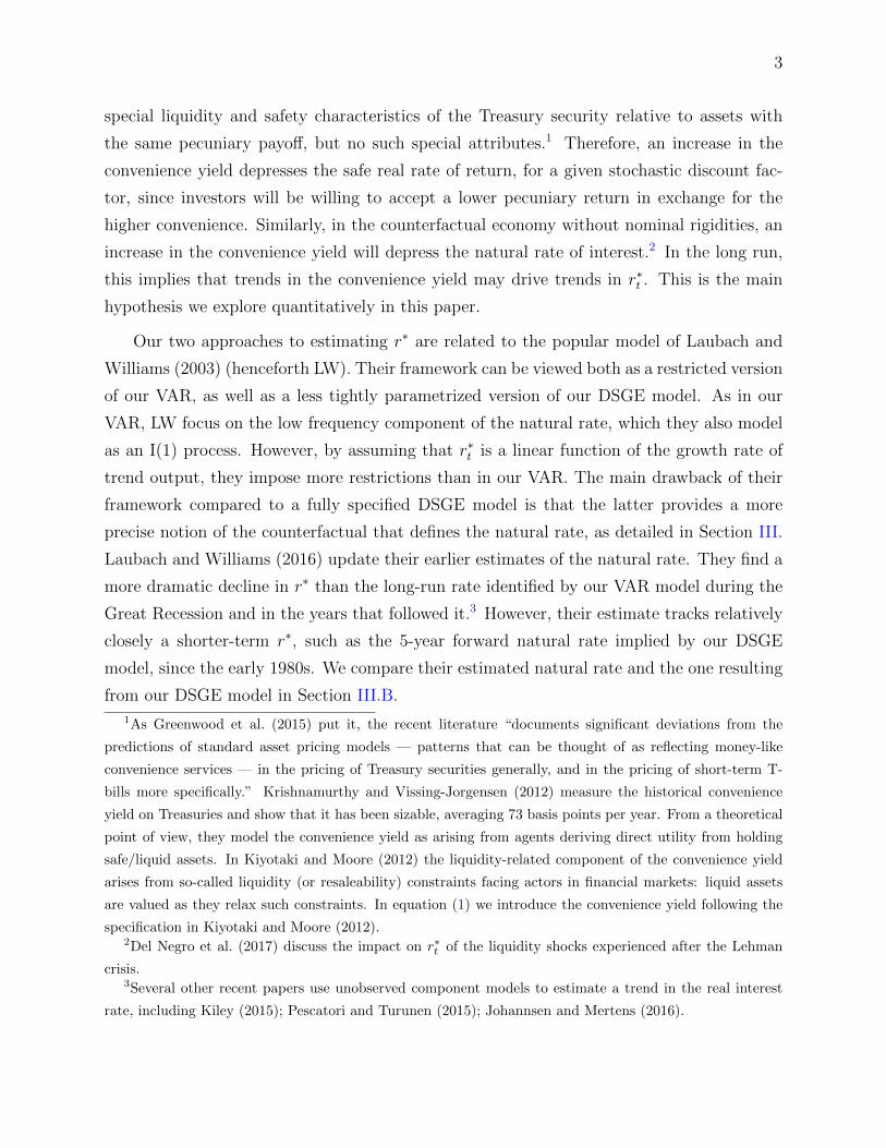
Results. The left panel of Figure 1 shows the estimates of rt. The dashed black line

shows the posterior median of rt while the shaded areas show the 68 and 95 percent posterior

coverage intervals (this convention applies to all latent variables shown below). rt rises from

the 1960s to the early 1980s, remains roughly constant until the late 1990s, and then begins

obtained from the SPF and are available once a year starting in 1992Q1. The 20-year Treasury constant

maturity rate is not available from 1987Q1 to 1993Q3. For this period, following Haver Analytics, we use

instead an average of the 10 and 30-year Treasury constant maturity rates (GS10 and GS30, respectively).

We use quarterly averages for all variables that are available at higher frequency than quarterly.20Results with a tighter prior of 1/400 for the variance of the inflation trend only change in that the trend

in inflation does not rise as much as long-run inflation expectations in the mid-1970s, but are otherwise very

similar to the ones shown here.21Our prior for the variance Σε is a very uninformative Inverse Wishart distribution centered at a diagonal

matrix with unitary elements (except for inflation, for which the diagonal element is 2, and expectations, for

which the variance is .5; these numbers reflect presample variances, except for expectations which are not

available) with just enough degrees of freedom (n+ 2) to have a well-defined prior mean. We do not use the

“co-persistence” or “sum-of-coefficients” priors of Sims and Zha (1998).

14

to decline. This result is consistent with previous findings in the literature. In addition to

LW, Bauer et al. (2012, 2014); Christensen and Rudebusch (2016), using a term structure

model; Crump et al. (2016), using data on survey expectations; and Lubik et al. (2015),

using a time-varying parameter VAR, also find that long-term forward rates have fallen

substantially over the past twenty years. The median decline in rt from 1998Q1 to 2016Q4

is about one-and-a-quarter percentage points, as shown in the first column of Table 1, from

2.36 to 1.06 percent. This decrease is significant, in that the 95 percent credible intervals

range from -.43 to -2.07 percent. The left panel also shows the short-term rate R1,t and the

long-run expectations for the short-term rate Re1,t, both expressed in deviations from long-

run inflation expectations πet so that trends in the real variables become more apparent.22 rt

declines since the late 1990s along with the decline in long-term expectations for the short-

term real rate Re1,t− πet . Toward the end of the sample the trend remains above the data for

Re1,t−πet , which is arguably reasonable in light of the fact that these 10-year averages partly

reflect cyclical movements – e.g., the slow renormalization of real rates in the aftermath of

the crisis. It is also apparent from the figure that the use of long-run short-rate expectations

helps in terms of the inference on the trend, as the bands for rt get considerably narrower

when these data become available (the bands become somewhat wider again in the ZLB

period as we are not using data on the short-term rate during this period).

The right panel of Figure 1 shows the data, πt (dotted blue line), and πet (solid blue line),

together with the trend πt. We find that πt appears to capture well the trend in inflation

and essentially coincides with long-run inflation expectations, whenever these are available,

even though the model only imposes that πt, and πet share a common trend.

22The time series for R1,t − πet begins in 1970 simply because long-run inflation expectations were not

available before then. Figure A1 in the Appendix shows the estimated trends in the term premium together

with the term spread R80,t − R1,t. Figure A2 shows all the data yt used in the estimation together with

Λyt and yt, the non-stationary and stationary components, respectively. The figure shows that the model

fits the trends in the data reasonably well, including those in the 20-year yield, in that the yt’s do indeed

look stationary. In the aftermath of the Great Recession, however, all of the stationary components are

persistently negative, including those for inflation and long-run rates expectations. The model suggests that

the Great Recession has had a persistently negative effect on the cyclical component of inflation and interest

rates, possibly capturing headwinds to the recovery.

15

Figure 1: Trends and Observables, Baseline Model

rt, R1,t − πet , Re1,t − πet πt, πt, and πet

Q1-60 Q1-70 Q1-80 Q1-90 Q1-00 Q1-10-1

0

1

2

3

4

5

6

7

Q1-60 Q1-70 Q1-80 Q1-90 Q1-00 Q1-10

-5

0

5

10

Note: The left panel shows R1,t − πet (dotted blue line), and Re

1,t − πet (blue dots), together with the trend rt. The right panel

shows πt (dotted blue line), and πet (solid blue line), together with the trend πt. For each trend, the dashed black line shows

the posterior median and the shaded areas show the 68 and 95 percent posterior coverage intervals.

II.B Drivers of rt: The Role of the Convenience Yield

Trends in the Convenience Yield.

Model Specification. In this section we refine the approach outlined above with the goal of

assessing the component of long-term movements in r due to changes in the convenience

yield. In order to do that we bring into the analysis assets whose safety/liquidity attributes

are not the same as those of nominal Treasuries.

The Euler equation (9) implies that trends in rt are driven by trends in the convenience

yield CYt and in the stochastic discount factor Mt. In order to proceed we make the as-

sumption that the covariance between CYt and Mt is stationary and write:

rt = mt − cyt, (14)

where cyt = log(1 + CYt) and mt = −logMt. In addition, we assume that the trends cyt

and mt evolve independently from one another according to equation (3) (although shocks

to the trends are allowed to be correlated).

Using the above decomposition we can replace rt with mt− cyt in expressions (10), (12),

and (13). Implicitly this amounts to assuming that in the long run all Treasuries, regardless

of maturity, benefit in equal measure of the same safety and liquidity attributes as 3-month

bills (an assumption we discuss below). This implies that data on R1,t, R80,t, or Re1,t are of

no use in disentangling cyt from mt. In order to do that we need to consider assets who carry

16

less of a convenience yield than Treasuries. Krishnamurthy and Vissing-Jorgensen (2012) use

the spread between Baa corporate bonds and Treasuries to identify the convenience yield.

We follow their lead and augment the set of observables with the yield of Baa corporate

bonds, which we model as follows:

RBaat = mt − λBaacy cyt + dt + πt + tpt + RBaa

t , (15)

where 0 ≤ λBaacy < 1, indicating that Baa corporate bonds are less liquid/safe than Treasuries,

and where dt reflects trends in the actual default probability of corporate bonds. We use the

same term premium that we use in equivalent maturity Treasuries (following Krishnamurthy

and Vissing-Jorgensen, 2012, we use 20-year Treasury yields as the reference), which means

that we constrain the term premium to be the same, at least in the long run. In the reminder

of this section we will ignore dt, on the grounds that there is clear secular trend in the average

corporate default probability. In the robustness section we discuss the results of a model

that explicitly accounts for dt, and show that our results are even stronger.

From equations (15) and (12) it follows that the trends in the spread between Baa

corporate bonds yields and equivalent maturity Treasuries is given by

RBaat − R80,t = (1− λBaacy )cyt, (16)

which implies that trends in the spread reflect trends in the convenience yield. Specifically,

we will assume that λBaacy = 0, that is, that Baa corporates do not have any convenience yield

whatsoever. Given the measured difference in trends RBaat − R80,t between Baa corporate

bonds yields and equivalent maturity Treasuries this assumption is the most conservative in

terms of extracting cyt. We should also stress that our results focus on secular changes in

the convenience yield, as opposed to its level. The level of the Baa/Treasury spread may

be affected by factors other than safety and liquidity premiums (e.g., the average default

probability of corporate bonds). The key identifying assumption we use is that secular

changes in the spread primarily reflect secular changes in the convenience yield.

Equation (16) deserves additional comments. First, as explained very clearly in Kr-

ishnamurthy and Vissing-Jorgensen (2012) the spread RBaat − R80,t captures not just the

current value of the convenience yield, but rather the expected average convenience yield

throughout the remaining maturity of the bond. But this is precisely what we need since

we are after trends in the convenience yield. Second, we assumed that long-term Treasuries

benefit of the same convenience yield as short-term Treasuries. In making this assumption,

we are arguably underestimating the convenience yield on short-term Treasuries, which is

17

what we are after. All Treasuries are equally safe, irrespective of their maturity, hence it

is reasonable to assume that the component of the convenience yield deriving from safety

applies evenly across maturities. As for the component associated with liquidity, Greenwood

et al. (2015) provide some evidence that the liquidity premium is a decreasing function of

maturity. They compute what they call z-spreads, which capture deviations in the pricing

of Treasury Bills from the an extrapolation based on the rest of the yield curve, and argue

that these z-spreads, which are sizable, “reflect a money-like premium on short-term T-bills,

above and beyond the liquidity and safety premia embedded in longer term Treasury yields”

(pg. 1687). In conclusion, for these reasons we think that our assumption that the conve-

nience yields extracted from long-term Treasuries applies in the same measure to Treasury

Bills is conservative; it is an assumption nonetheless, and one should bear that in mind in

interpreting our results.

The system of equations given by (10)–(13) and (15) can be expressed as a VAR for yt =(πt, π

et , R1,t, R80,t, R

e1,t, R

Baat

)with common trends yt =

(rt, πt, cyt, tpt

).23 We use exactly the

same priors as described in Section II.A, except that since we decompose the trend rt into

two components, mt and cyt, we center the corresponding diagonal value of Σε to a number

that is 1/2 the value chosen for rt (we use 1/800 as opposed to 1/400).24

Results. The left panel of Figure 2 shows rt together the short-term rate R1,t and the

long-run expectations for the short-term rate Re1,t, both expressed in deviations from long-run

inflation expectations πet , similarly to the right panel of Figure 1. The time series of rt is very

similar to that shown in Figure 1, albeit not identical at the beginning of the sample (recall

we are now using a larger cross section of yields to pin down rt). In terms of the question

this paper addresses, the decline in rt from the late 1990s to the present is 1.27 percentage

points, the same as estimated before, as shown in the second column of Table 1. The other

two panels show that much of this decline is attributable to an increase in the convenience

yield, rather than to a fall in mt. The middle panel shows cyt, and the spread between Baa

securities and comparable Treasuries RBaat − R80,t. This spread has a clear upward trend,

especially starting right before the turn of the century, which is picked up by the estimate

23The Baa yield is available from FRED (mnemonic, Baa). As described in Krishnamurthy and Vissing-

Jorgensen (2012, pg. 262) “The Moody’s Baa index is constructed from a sample of long-maturity (≥ 20

years) industrial and utility bonds (industrial only from 2002 onward).” This series is available throughout

the whole sample, but ends in 2016Q3.24The initial condition cy0 is set at 1 using presample averages for the Baa/Treasury spread, and corre-

spondingly set m0 to 1.5 (r0 + cy0). The variance of the initial conditions is 1, as is the case for all other

trends.

18

Figure 2: Trends and Observables, Convenience Yield Model

rt, R1,t − πet , Re1,t − πet cyt, and RBaa

t −R80,t mt, and R1,t − πet − (RBaat −R80,t)

Q1-60 Q1-70 Q1-80 Q1-90 Q1-00 Q1-10-1

0

1

2

3

4

5

6

7

Q1-60 Q1-70 Q1-80 Q1-90 Q1-00 Q1-100

0.5

1

1.5

2

2.5

3

3.5

4

4.5

Q1-60 Q1-70 Q1-80 Q1-90 Q1-00 Q1-100

1

2

3

4

5

6

7

8

9

Note: The left panel shows R1,t − πet (dotted blue line), and Re

1,t − πet (blue dots), together with the trend rt. The middle

panel shows the Baa/Treasury spread RBaat − R80,t (dotted blue line), together with the trend cyt. The right panel shows

R1,t − πet − (RBaa

t − R80,t) (dotted blue line), together with the trend mt. For each trend, the dashed black line shows theposterior median and the shaded areas show the 68 and 95 percent posterior coverage intervals.

of cyt. Table 1 shows that the convenience yield increases by 92 basis points from 1998Q1

to 2016Q4, with 95 percent credible intervals ranging from 49 to 135 basis points. The right

panel shows the “real rate” R1,t − πet minus the spread RBaat − R80,t. It shows that there is

a fall in mt (the median decline is about 35 basis points) but is imprecisely estimated, as

the upper bound of the 68 percent credible interval is essentially 0. We should stress once

again that the reader should not focus on the level of mt and cyt, but on their changes. Our

statement is not “Were it not for the convenience yield from liquidity/safety, the secular

components of real rates would be x percent” but rather “Much of the decline in rates over

the past twenty years is due to the convenience yield.” This is because the level of the

spread RBaat −R80,t is affected by factors — mostly the probability of default — other than

the convenience yield.25

Another perspective on what we find is that the secular decline in real rates for un-

safe/illiquid securities has been much less pronounced, if it has taken place at all, than

that for safe/liquid securities. As discussed in the introduction, the trend increase in the

safety/liquidity convenience yield since the late 1990s is very much in line with the narrative

put forth by Caballero (2010) and the “safe assets” literature more broadly. The Asian crisis

first resulted in excess supply of savings which, being institutional (that is, intermediated via

25Figure A3 in the Appendix shows the remaining estimated trends (πt and tpt) along with the relevant

data. Figure A4 shows all the data yt used in the estimation together with Λyt and yt, the non-stationary

and stationary components, respectively.

19

central banks), was naturally directed toward safe and liquid assets. The NADSAQ crash

further rendered safe assets more attractive. The housing boom and the related creation of

allegedly safe securities partly met this increased demand, but this suddenly came to a halt

with the housing crisis and the Great Recession, which resulted in an additional increased

demand, and reduced supply, of safe and liquid assets.

Trends in the Compensation for Safety and Liquidity.

Model Specification. Following Krishnamurthy and Vissing-Jorgensen (2012), we decompose

the convenience yield (1 + CYt) into two parts, one due to liquidity (1 + CY lt ) and one to

safety (1 + CY st ), and write the Euler equation for a safe/liquid security as

Et[(1 + rt)(1 + CY lt+1)(1 + CY s

t+1)Mt+1] = 1.

Under the assumption that the covariances between CY lt , CY s

t , and Mt are stationary we

obtain that:

rt = mt − cylt − cyst . (17)

The distinction between liquidity and safety has two benefits. First, from an economic point

of view, it allows us to disentangle the importance of the two components in explaining

trends in r∗. In order to do so, of course, we have to be able to identify the two trends

separately. Following once again Krishnamurthy and Vissing-Jorgensen (2012) we do so by

bringing into the analysis the Aaa corporate yield, an index of securities that virtually never

default, and hence carry as much of a safety discount as Treasuries, but are less liquid than

Treasuries, and hence enjoy less of a liquidity premium. We therefore write:

RAaat = mt − λAaal cylt − cyst + πt + tpt + RBaa

t , (18)

RBaat = mt − λAaal cylt − λBaas cyst + πt + tpt + RBaa

t , (19)

where 0 ≤ λAaal < 1 and 0 ≤ λBaas < 1, indicating that both Aaa and Baa corporate bonds

are less liquid than Treasuries (we assume that their degree of illiquidity is the same, hence

λBaal = λAaal ), and that Baa corporate bonds are less safe than Treasuries. From equations

(18), (19) and (12) it follows that

RAaat − R80,t = (1− λAaal )cylt,

RBaat − RAaa

t = (1− λBaas )cyst .

As before, we will make the conservative assumptions that Baa bonds earn no safety and

liquidity premium whatsoever, and that Aaa bonds are completely illiquid. These assump-

20

tions are conservative in the sense that they minimize time variation in the trends cylt and

cyst given the observed trends in the spreads RAaat − R80,t and RBaa

t − RAaat .

The system of equations given by (10)–(13) and (19)-(18) can be expressed as a VAR

for yt =(πt, π

et , R1,t, R80,t, R

e1,t, R

Aaat , RBaa

t

)with common trends

(rt, πt, cy

st , cy

lt, tpt

).26 We

use exactly the same priors as described above, except that since we decompose the trend

cyt into two components, cyst and cylt, we center the corresponding diagonal values of Σε to

a number that is 1/2 the value chosen for cyt (we use 1/1600 as opposed to 1/800).27 This

obviously makes it harder to find a trend in these convenience yields.

Results. Figure 3 shows the trend rt and its decomposition between trends in the con-

venience yield for safety and liquidity cyt = cylt + cyst (we are actually plotting −cyt) and

the stochastic discount factor mt. The estimates for rt appear in all three panels, and the

level of both −cyt and mt are normalized so that in 1998Q1 the three series coincide (at the

median), so that the source of the post-1998 decline in rt is more apparent. The estimates

of rt are virtually the same as those shown in Figures 2, and have rt fall by 1.3 percentage

points between 1998Q1 and 2016Q4 (see column 3 of Table 1). Again, this decline is pre-

cisely estimated. The middle panel shows that roughly one percentage point of this decline

is attributable to an increase in the convenience yield. The converse of the convenience yield

(−cyt) falls by one percent, and the decrease is very precisely estimated, with the 68 and

95 percent posterior coverage intervals ranging from -.75 to -1.18 percent and from -.53 to

-1.40 percent, respectively. mt also declines in the new century, by about 30 basis points,

but its estimates are much more uncertain: the 68 percent intervals of the estimated fall in

mt range from -0.01 to -.65 percent.

Figure 4 shows the estimated trends in the overall convenience yield cyt, and the conve-

nience yields attributed to safety (cyst) and liquidity (cylt), along with the information that

the model uses to extract these trends.28 The left panel shows cyt = cyst + cylt, and the

spread between Baa securities and Treasuries RBaat − R80,t. Again, in spite of the fact that

26The Aaa yield is also available from FRED (mnemonic, AAA) and has similar characteristics as the Baa

index in terms of maturity. This series is available throughout the whole sample, but ends in 2016Q3.27The initial conditions cys0 and cyl0 are set at .75 and .25 using presample averages for the Baa/Aaa and

the Aaa/Treasury spreads. The variance of the initial conditions is 1, as is the case for all other trends.28Figure A5 in the Appendix shows the remaining estimated trends (πt, rt, mt, and tpt) along with the

relevant data. Figure A7 shows all the data yt used in the estimation together with Λyt and yt, the non-

stationary and stationary components, respectively. Figure A6 in the Appendix shows the prior and posterior

distributions of the standard deviations of the shocks to the trend components—the diagonal elements of

the matrix Σe.

21

Figure 3: rt, cyt, and mt

rt −cyt mt

Q1-60 Q1-70 Q1-80 Q1-90 Q1-00 Q1-100

0.5

1

1.5

2

2.5

3

3.5

4

Q1-60 Q1-70 Q1-80 Q1-90 Q1-00 Q1-100

0.5

1

1.5

2

2.5

3

3.5

4

Q1-60 Q1-70 Q1-80 Q1-90 Q1-00 Q1-100

0.5

1

1.5

2

2.5

3

3.5

4

Note: The dashed black line shows the posterior median and the shaded gray areas show the 68 and 95 percent posteriorcoverage intervals for rt. The dashed orange line shows the posterior median and the shaded orange areas show the 68 and 95percent posterior coverage intervals for −cyt (middle panel) and mt (right panel).

the trends cyst and cylt are now separately estimated, the inference for cyt is broadly similar

to that shown in Figure 2. The middle panel shows cyst and the spread between Baa and Aaa

bonds RBaat − RAaa

t . The trend in this spread, according to the model, has less of a secular

increase in the overall sample than the overall convenience yield. The trend in the safety

premium increases in the 1970s, reaches a pick in the early eighties, declines progressively

until the NASDAQ crash, and finally increases by a little less than 50 basis points until the

end of the sample. The estimated increase in the safety convenience yield between 1998Q1

and 2016Q4 is 45 basis points, and is very significantly different from zero.

The right panel shows cylt, and the spread between Aaa securities and Treasuries RAaat −

R80,t. The trend cylt has a more pronounced secular increase since the early 1980s.29 From

the perspective of the focus of the paper — the sources of the decline in real rates since

the 1990s — the right panel shows an increase in cylt by about 50 basis points since 1998

(see column 3 of Table 1).30 Much of this increase occurred during and after the financial

crisis. This is not surprising, because the liquidity shock in the aftermath of the Lehman

29While the transitory spikes in the convenience yield for liquidity are easily explained by financial events

(e.g., the stock market crash of 1987, the burst of the 1990s stock market bubble and September 11, the

Lehman crisis), this secular increase is for us not straightforward to explain, but we find it an interesting

question for future research. One possibility is that it is related to the growth of the shadow banking system

documented in Adrian and Shin (2009, 2010).30Note that the high frequency spike in illiquidity occurred during the financial crisis does not seem to

play an important role in the extraction of the trend; in other words, the increase in the compensation for

liquidity appears to be mostly driven by the low frequency movements in the spreads.

22

Figure 4: Trends in Compensation for Safety and Liquidity, and Observables

cyt, and RBaat −R80,t cyst , and RBaa

t −RAaat cylt, and RAaa

t −R80,t

Q1-60 Q1-70 Q1-80 Q1-90 Q1-00 Q1-100

0.5

1

1.5

2

2.5

3

3.5

4

4.5

Q1-60 Q1-70 Q1-80 Q1-90 Q1-00 Q1-100

0.5

1

1.5

2

2.5

3

Q1-60 Q1-70 Q1-80 Q1-90 Q1-00 Q1-100

0.2

0.4

0.6

0.8

1

1.2

1.4

1.6

1.8

Note: The left panel shows the Baa/Treasury spread RBaat −R80,t (dotted blue line), together with the trend cyt. The middle

panel shows the Baa/Aaa spread RBaat − RAaa

t (dotted blue line), together with the trend cyst . The right panel shows the

Aaa/Treasury spread RAaat −R80,t (dotted blue line), together with the trend cylt. For each trend, the dashed black line shows

the posterior median and the shaded areas show the 68 and 95 percent posterior coverage intervals.

crisis drastically curtailed the supply of liquid assets (as several asset classes became less

liquid; see for instance Del Negro et al., 2017; Gorton and Metrick, 2012) and at the same

time increased its demand. In addition, the regulatory changes after the crisis (see the

liquidity requirements for financial institutions under Basel III; Basel Committee on Banking

Supervision, 2013) also led to an increased demand for liquid assets, as well as a decline in the

supply of liquid liabilities from the financial system. In conclusion, we find that the increase

in the convenience yield since the late 1990s is roughly evenly split between compensation

for safety and liquidity.

II.C The Role of Consumption

Model Specification. The VAR specifications that we have considered so far have all been

agnostic on the fundamental determinants of the trends in the stochastic discount factor mt.

We chose this approach because there is no consensus in the literature on how to model this

variable. Many asset pricing theories, however, connect the pricing kernel to some function

of consumption growth. This list includes the consumption Euler equation that holds in the

DSGE model of the next section. These theories, in fact, are the basis for the often discussed

relationship between trends in rate of returns and in the growth rate of the economy (e.g.

Laubach and Williams, 2003; Hamilton et al., 2015).

23

This section explores this relationship by including a measure of per capita consumption

growth in the VAR. This model is an extended version of the baseline specification of Section

II, in which mt is decomposed into two factors. The first factor, denoted by gt, is common

between the trends in mt and in the growth rate of per capita consumption, which we call

∆ct. Motivated by the fact that trends in mt may in principle be driven by factors that are

not associated with consumption, we also introduce a residual factor, βt, so that

mt = gt + βt. (20)

In addition, we do not impose that gt is the same as the trend in overall consumption growth,

as would be the case in a textbook version of the Euler equation with log utility. Instead,

we allow for another trend in consumption growth, or

∆ct = gt + γt.

This specification admits the possibility that the relevant consumption pricing factor for

interest rates is not aggregate consumption, but possibly a subset of consumption with

a different trend from the aggregate. This would be the case, for instance, in a limited

participation model in which only a subset of consumers have access to financial markets

and the low frequency component of their consumption growth is different from that of non-

participants (e.g., Vissing-Jorgensen, 2002). Given the steady growth in inequality over the

last few decades, such a persistent divergence in the consumption prospects of richer asset

holders and poorer households excluded from financial markets seems plausible.

In sum, we augment the system of equations given by (10)–(13) and (18)-(19) with an

equation for consumption growth

∆ct = gt + γt + ∆ct, (21)

and set mt = gt + βt in all the equations involving mt.31 In terms of priors, we want to

allow ample room for the trend in consumption growth gt to account for the decline in rt.

Therefore, we assume that its prior standard deviation is four times as large as that of cyst

and cylt, which implies a value of 1/400 for the corresponding diagonal element of the matrix

Σe. We also assume the same prior for γt, while the standard deviation of βt is set to 1/8 of

that of gt.32 All other priors are the same as in the baseline model.

31We use the same measure of real per capita consumption as in the DSGE model, namely Personal

Consumption Expenditures divided by the GDP deflator and by a smoothed version of population. See the

DSGE data Appendix for more details. Consumption growth is quarterly annualized.32The initial condition γ0 is calibrated by splitting in two the average growth rate of per capita consumption

in the 1950s. The initial conditions γ0 and β0 are set to zero.

24

Figure 5: Consumption Growth and Its Trend

Q1-60 Q1-70 Q1-80 Q1-90 Q1-00 Q1-10-5

-4

-3

-2

-1

0

1

2

3

4

5

Note: The left panel shows ∆ct (4-quarter average; dotted blue line) and ∆ct = gt + γt. For the trend, the dashed black lineshows the posterior median and the shaded areas show the 68 and 95 percent posterior coverage intervals.

Results. Figure 5 shows the 4-quarter average of the growth rate of per capita consump-

tion together with its trend ∆ct = gt + γt. The figure shows that the estimated trend in

consumption growth has fallen over the past twenty years. This decline has been notable,

as shown in column 4 of Table 1. The median estimate is .80 percentage point, although it

is imprecisely estimated. Table 1 also shows that the component attributable to gt, which

is the part of the trend in consumption growth that affects the interest rate, is around 55

basis points at the posterior median, and it is also surrounded by significant uncertainty.

Nonetheless, the estimated decline in rt — 1.40 percent points — and the increase in the

convenience yield — 0.78 percentage points — are close to the figures shown before, and are

still precisely estimated.33 In sum, the increase in the convenience yield still accounts for

the majority of the overall secular trend decline in rt.34

Results were very similar in a model in which we substituted the growth rate of con-

sumption with that of labor productivity among the observables. The motivation for also

33Figure A8 in the Appendix shows the remaining estimated trends (πt, rt, mt, tpt, cyst , and cylt) along

with the relevant data. Figure A9 shows all the data yt used in the estimation together with Λyt and yt, the

non-stationary and stationary components, respectively.34We also estimated a more restricted model with a common trend between aggregate consumption and

the interest rate — that is, eliminating γt. In that model, the trend in consumption moves much less, and

the effects on mt are smaller, suggesting that the restriction that all of the trend in consumption growth

translates into secular changes in the discount factor is at odds with the data. Otherwise the results are quite

similar to those just discussed. We also tried to estimate the intertemporal elasticity of substitution — that

is, modifying (20) as mt = σ−1gt + βt. This only resulted in more uncertain estimates of the decline in mt.

This possibly reflects the well-know difficulties in pinning down the intertemporal elasticity of substitution.

25

experimenting with this specification comes from the neoclassical growth model, in which

the interest rate, productivity growth and consumption growth are all tied together along

the balanced growth path. Therefore, productivity growth provides an alternative source of

information on the trend growth rate of the economy. The two trends might not coincide for

several reasons, including persistent movements in the current account in an open economy,

as well as trends in the labor force participation rate that drive a wedge between the growth

rates of population (in the denominator of per capita consumption) and of hours worked (in

the denominator of labor productivity). Both these phenomena have been observed in the

United States since the 1990s and they are often mentioned as possible secular drivers of the

decline in interest rates that has occurred over the same period. As shown in column 4 of

Table A1 in the Appendix, the estimated trend decline in the real interest rate in this model

is centered around 1.64 percentage points, the highest value of all the models we estimated.

Of this decline, 89 basis points are accounted for by the increase in the convenience yield,

and another 68 by the decline in the trend growth rate of productivity. As before, the former

contribution is very tightly estimated, while the latter is quite uncertain.

In summary, the results of this augmented model corroborate our conclusion that the

increase in the convenience yield has been a crucial factor in the secular decline of Treasury

yields. In addition, the model suggests that the concomitant fall in the trend growth rate

of economic activity — measured either in the form of consumption or of labor productivity

— also played a relevant role, although this conclusion is subject to significant uncertainty.

II.D Robustness

This section considers some variants to our benchmark specification — the model with

convenience from both safety and liquidity.

Accounting for Trends in Corporate Default.

Figure 6 shows the median distance to default (DD) in the non-financial corporate sector used

in Gilchrist and Zakrajsek (2012) — the higher DD the lower the default probability.35 This

measure has a clear upward trend since the late 1990s, implying that there is, if anything, a

secular decrease in the default probability, which is why we did not include in the benchmark

models. For completeness, here we estimate a model where we extract trends in the distance

35These are the data shown in Figure 2 of Gilchrist and Zakrajsek (2012). We are very grateful to Egon

Zakrajsek for providing us with updated estimates.

26

Figure 6: Distance to Default

Q1-77 Q1-87 Q1-97 Q1-07

3

4

5

6

7

8

9

10

11

12

Note: The figure shows the median distance to default (DD) in the non-financial corporate sector used in Gilchrist and Zakrajsek(2012).

to default Dt from the data shown in Figure 6, and include them in the equation for the Baa

yield, which becomes

RBaat = mt − γdl Dt + πt + tpt + RBaa

t , (22)

where γd is estimated (we use an exponential distribution with mean 1/10 as the prior).36

Table A1 in the Appendix shows that the estimated increase in the convenience yield is

stronger than reported in Table 1, about 1.4 percentage points, and remains precisely esti-

mated.

Loose Prior on the Trend.

Our main results is that trends in the convenience yield account for a large chunk of the

decline in rt, while the effect of changes in the trend for the discount factor mt is not as

large, and is quite imprecisely estimated. One natural objection to our argument is that our

prior on the standard deviation of the trends innovation is too conservative and too tight. If

we had a looser prior, we may possibly find more evidence of a trend in rt and consequently

mt.

Figure 7 dispels this notion. This figure shows the outcome of reestimating the model of

36The prior mean for γd is loosely based on the results of the panel regressions reported in Gilchrist and

Zakrajsek (2012), who estimate the effect of the distance to default on corporate spreads. The prior on the

variance of the trend Dt (that is, the corresponding diagonal element of the matrix Σe) is 1/400, which

is the same prior we used for rt in the first model. The exponential distribution with parameter γ−1 is

p(γ; γ−1) = γ−1 exp(−γ−1γ)Iγ ≥ 0, where I. is an indicator function.

27

Figure 7: Trends and Observables, Loose Prior on the Trend

rt, R1,t − πet , Re1,t − πet cyt, and RBaa

t −R80,t mt, and R1,t − πet − (RBaat −R80,t)

Q1-60 Q1-70 Q1-80 Q1-90 Q1-00 Q1-10-1

0

1

2

3

4

5

6

7

Q1-60 Q1-70 Q1-80 Q1-90 Q1-00 Q1-100

0.5

1

1.5

2

2.5

3

3.5

4

4.5

Q1-60 Q1-70 Q1-80 Q1-90 Q1-00 Q1-100

2

4

6

8

10

Note: The left panel shows R1,t−πet (dotted blue line), and Re

1,t−πet (blue dots), together with the trend rt. The middle panel

shows the Baa/Treasury spread RBaat − R80,t (dotted blue line), together with the trend cyt. The right panel showsR1,t −

πet − (RBaa

t −R80,t) (dotted blue line), together with the trend mt. For each trend, the dashed black line shows the posteriormedian and the shaded areas show the 68 and 95 percent posterior coverage intervals.

Section II.B loosening the prior on variance-covariance matrix as much as possible (we use 8

degrees of freedom, barely enough so that the prior has a well defined mean, as opposed to

the 100 used in the baseline specification). The result is that the trend is no longer a trend

in the sense that it also captures high frequency fluctuations in the observables — which is

why we think the original tight prior is appropriate. But the broad contours of the results

are the same: cyt trends upward while mt does not move much.37

Inflation Affecting the Nominal Term Premium.

As anticipated, we also allow for the possibility that trends in inflation affect the nominal

term premium — that is, we model the term premium as the sum of an exogenous component

tpt and a component γtpπt, where γtp is estimated (we use an exponential distribution with

mean 1/10 as the prior). This specification is motivated by the work of Wright (2011), who

found a positive correlation between the level of the nominal term premium and the volatility

of inflation. Here, we use the level of inflation as a proxy for the latter. We therefore replace

tpt with tpt + γtpπt in equations (12), (18), and (19). The results under this specification

are nearly identical to those shown in Section II.B and therefore are relegated to the online

appendix (Figure A11; Figure A10 shows the posterior distribution of γtp).

37We obtain similar results when we instead quadruple the variance of the trend innovations, but leave

intact the number of degrees of freedom.

28

Callability.

Many corporate bonds are callable, while Treasuries are not (at least since 1985). One

may wonder whether secular changes in the value of the call option drive secular changes

in the spread. Fortunately, there are other spreads mainly reflecting liquidity other than

the Aaa/Treasuries spread. The Refcorp/Treasury spread is one of them. This spread,

according to Longstaff et al. (2004), is mostly (if not entirely) due to liquidity as Refcorp

bonds are effectively guaranteed by the U.S. government, are subject to the same taxation

and, importantly, to the best of our knowledge they are not callable.38

Figure 8: Trends in the Liquidity Convenience Yield and the Refcorp Treasury Spread

Q1-60 Q1-70 Q1-80 Q1-90 Q1-00 Q1-10

0

0.25

0.5

0.75

1

1.25

1.5

1.75

2

-0.5

-0.25

0

0.25

0.5

0.75

1

Note: The figure shows the estimated trend in the liquidity convenience yield cylt (the dashed black line shows the posteriormedian and the shaded areas show the 68 and 95 percent posterior coverage intervals; left axis), the Aaa/Treasury spread

RAaat −R80,t (dotted blue line; left axis) and the Refcorp/Treasury spread (solid purple line; right axis). See footnote 38 for a

description of how this spread is constructed.

Figure 8 plots the estimated trend in the liquidity convenience yield cylt shown in the

right panel of Figure 4 together with daily data on the Refcorp/Treasury spread collected

by Del Negro et al. (2017) from 4/16/1991 to 9/06/2014. The figure shows that the trend

in liquidity estimated using the Aaa/Treasury spread matches very well the trends in the

Refcorp/Treasury spread, whenever this is available. In addition to suggesting that callability

38 Refcorp bonds differ from most other agency bonds in that their principal is fully collateralized by

Treasury bonds and full payment of coupons is guaranteed by the Treasury under the provisions of the

Financial Institutions Reform, Recovery, and Enforcement Act of 1989. Longstaff et al. (2004) does not

mention callability as a feature of these bonds. Lehman Brother’s “Guide to Agency and Government-

Related Securities” does not mention callability in reference to Refcorp bonds, while it discusses callability

for other agency securities. As in Longstaff et al. (2004), we measure the spread by taking the differences

between the constant maturity 10-year points on the Bloomberg fair value curves for Refcorp and Treasury

zero-coupon bonds. The Bloomberg mnemonics are ‘C091[X]Y Index’ and ‘C079[X]Y Index’, respectively,

where [X] represents the maturity.

29

is not the driving force behind secular movements in the Aaa/Treasury spread, Figure 8

provides important external validation to our analysis.39

III The Natural Rate of Interest in DSGE Models

Our analysis so far focused on long-run trends in r∗t and on the factors that drive them.

However, the natural rate of interest also fluctuates over the business cycle. This section

presents estimates of r∗t based on an empirical medium-scale Dynamic Stochastic General

Equilibrium (DSGE) model that features nominal price and wage rigidities, as well as a host

of real and financial frictions. Within this New Keynesian environment, we define r∗t as the

real interest rate that would prevail in equilibrium in the absence of sticky prices and wages,

as discussed in the introduction.40

This particular notion of r∗t is a useful tool in macroeconomic and monetary analysis for

several related reasons. First, the natural rate does not depend on monetary policy. In the

equilibrium without nominal rigidities, monetary policy is neutral, in the sense that it does

not affect any real variable, including the real interest rate.41 Therefore, the natural rate

answers the question: what would the real interest rate be, “without” monetary policy?

Second, the gap between actual interest rates and their natural level is a more appropriate

measure of the impetus (or restraint) imparted by monetary policy to aggregate demand

than the level of the policy rate itself, as further discussed in Section III.B. In Wicksell’s

own words, “it is not a high or low rate of interest in the absolute sense which must be

39An alternative approach to addressing the issue of callability is the one taken by Gilchrist and Zakrajsek

(2012) in the construction of the excess bond premium, who use a panel regression where they regress

individual corporate spreads on individual measures of default probability as well as variables that likely

capture the value of the call option. While this micro-level approach has several advantages relative to our

aggregate approach — especially in terms of the exact computation of the spreads in terms of maturity and

the removal of default probability — it has one important drawback from our perspective: in order to remove

the call option, the spreads are regressed on the level of the interest rate, among other variables, thereby

removing the very trends we are interested in.40Neiss and Nelson (2003) were the first to evaluate the properties of the natural rate in a calibrated DSGE

model. Edge et al. (2008), Justiniano and Primiceri (2010), Barsky et al. (2014), and Curdia et al. (2015)

do so in estimated models.41This statement holds in the model proposed below, but it might need to be qualified in other environ-

ments. Depending on the exact specification of the financial and real frictions, monetary policy might affect

real variables even in the absence of nominal rigidities. However, these effects tend to be quantitatively

limited in empirical models.

30

regarded as influencing the demand for raw materials, labour, and land or other productive

resources, and so indirectly as determining the movement of prices. The causality factor is

the current rate of interest on loans as compared to [the natural rate].”

This property of the natural rate does not imply that closing the interest rate gap is

optimal. This is the case only in extremely simple models that do not feature a trade-

off between real and nominal stabilization. In these models, closing the interest rate gap

stabilizes the output gap, and at the same time inflation. In larger, more realistic DSGE

models, this “divine coincidence” (Blanchard and Galı, 2007) between price stability and

full employment does not hold. Nonetheless, a monetary policy strategy in which the real

policy rate tracks the natural rate generally promotes stable inflation and economic activity

even in those models, providing a more explicitly normative rationale for using estimates of

the natural rate as an input in monetary policy making.42

The DSGE perspective on r∗t described above is complementary to that explored in the

first part of the paper. While the VAR only provides an estimate of the low frequency

component of r∗t , a fully specified DSGE model gives us the entire time-path of r∗t . This is

especially relevant in a policy context, This is especially relevant in a policy context, where

estimates of r∗t might be used to inform decisions on the appropriate level of the policy rate.

Of course, the flip side of this more comprehensive view of the movements in r∗t provided

by the DSGE approach is that inference is conditional on the exact structure of the DSGE

model. As such, it is more likely to be affected by model misspecification than the VAR

estimates. However, one of the key findings of our DSGE exercise is that its conclusions

in terms of low frequency fluctuations in r∗t agree with those of the reduced form exercise.

The fact that the DSGE model can capture these low frequency movements is a surprising

result in itself. Moreover, the two approaches also agree that the rise in the convenience

yield is the source of this secular decline in r∗t , as illustrated in Section III.B. Also, we find

that the natural rate plunged to its historical lows during the Great Recession, making the

lower bound on nominal interest rates bind, and hence severely impairing the ability of the

Federal Reserve to stabilize the economy through its conventional policy tool, as we discuss

further in Section III.B.43

42For instance, Justiniano et al. (2013) find that the there is a minimal trade-off between nominal and real

stabilization in an estimated model similar to the one used here, approximating the divine coincidence that

holds exactly in much simpler environments.43 We should note that studies based on a variety of empirical DSGE models tend to deliver a fairly

consistent view of the business cycle fluctuations in r∗t , even if their estimates do not coincide at any given

point in time (see for instance Figure 1 in Yellen (2015)).

31

III.A DSGE model

The DSGE model considered here is a version of the FRBNY DSGE model described in

Del Negro et al. (2015). It builds on the model of Christiano et al. (2005) and Smets and

Wouters (2007), and expands it with various features, most notably financial frictions simi-

larly to Bernanke et al. (1999b) and Christiano et al. (2014). At the core of the model lies

a frictionless neoclassical structure in which monetary policy has no effects. This neoclas-

sical core is augmented with frictions such as stickiness of nominal prices and wages (i.e.,

nominal frictions), various real frictions (such as adjustment costs of capital) and financial

frictions that interfere with the flow of funds from savers to borrowers. In addition, the

model includes several structural shocks which are the ultimate causes of economic fluctua-

tions, such as shocks to productivity, the marginal efficiency of investment (e.g., Greenwood

et al. (1998), Justiniano et al. (2010)), and price and wage markup shocks. We also allow

for shocks to liquidity, safety, credit premia in line with the empirical model of Section II, as

well as anticipated policy shocks as in Laseen and Svensson (2011) to account for the zero

lower bound on nominal interest rates and forward guidance in monetary policy. The equi-

librium conditions are approximated around the non-stochastic steady state, and we express

all variables in (log) deviations from that steady state. A complete model specification is

detailed in Appendix B. Here, we focus the discussion on the parts of the model most closely

related to the natural rate of interest and its drivers.

We include two types of wedges between the Treasury rate and the rate at which corpora-

tions finance their investment.44 The first wedge arises from financial frictions a la Bernanke

et al. (1999a), which we model building on the work of Christiano et al. (2003), De Graeve

(2008), and Christiano et al. (2014).45 The second wedge arises exogenously and captures

the convenience yield — the fact that investors prefer to hold Treasuries over alternative

assets.46 These wedges affect the spread between corporate bond yields and Treasury yields

44Wu and Zhang (2016) also model the spread between private and government bonds in the context of a

New Keynesian model.45We assume that banks collect deposits from households and lend to entrepreneurs who use these funds

as well as their own wealth to acquire physical capital, which is rented to intermediate goods producers.

Entrepreneurs are subject to idiosyncratic disturbances that affect their ability to manage capital. Their

revenue may thus turn out to be too low to pay back the loans received by the banks. The banks therefore

protect themselves against default risk by pooling all loans and charging a spread over the deposit rate.46We model the convenience yield as a simple transaction cost/subsidy, following Smets and Wouters

(2007). Fisher (2015), following Krishnamurthy and Vissing-Jorgensen (2012), models it by including Trea-

sury bonds in households’ preference. Our transaction “subsidy” can be recast as a linear utility benefit

32

according to the (linearized) equation

IEt

[Rkt+1 −Rt

]= cyt + ζsp,b

(qkt + kt − nt

)+ σω,t, (23)

where IEtRkt+1 is the entrepreneurs’ expected (short-term) return on capital, Rt is the 3-

month Treasury bill rate, cyt is the wedge arising from the convenience yield, the term

qkt + kt − nt captures the entrepreneurs’ leverage (i.e. the value of capital qkt + kt relative

to net worth nt), and σω,t consists of Christiano et al. (2014)’s “risk shocks” — that is,

mean-preserving changes in the cross-sectional dispersion of entrepreneurial ability.

Two comments are in order regarding the convenience yield. First, it is assumed to be

exogenous, unlike in the models of Kurlat (2013), Bigio (2015), or Del Negro et al. (2017).

Although this is a theoretical limitation of our approach, it is functional to our empirical aim

to use the DSGE model to map the effects of changes in cyt on the macroeconomy, and on

r∗t in particular. Second, unlike in the papers just mentioned, in our model’s counterfactual

economy without nominal rigidities changes in cyt affect the real rate on Treasuries, but have

no effect on allocations. This “neutrality” of convenience yield shocks in the flexible price

economy implies that in the actual economy, monetary policy could in principle completely

isolate the economy from fluctuations in cyt by adjusting the policy rate appropriately. This

is a strong assumption, but one with some support: Del Negro et al. (2017) find that indeed

monetary policy can undo most of these effects.

We assume that cyt contains both a liquidity component cylt and a safety component cyst

cyt = cylt + cyst , (24)

which we identify through the same spreads used in Section II.B—the spreads between Aaa

and Baa corporate bonds and 20-year Treasuries. The former, which we assume mainly

reflects liquidity, is modeled as

Aaa − 20-year Treasury Spread = cyl∗ + IEt

[1

80

79∑j=0

cylt+j

]+ eAaat ,

while the latter, which reflects both liquidity and safety, as well as the actual probability of

default, is modeled as

Baa − 20-year Treasury Spread = cyl∗ + cys∗ + SP∗ + IEt

[1

80

79∑j=0

Rkt+j+1 −Rt+j

]+ eBaat ,

from holding Treasuries, as in Anzoategui et al. (2015).

33

where the terms IEt

[Rkt+j+1 −Rt+j

]include all the components included in expression (23).

These equations highlight that measured spreads are between long-term yields. There-

fore, in the model, they capture expectations of future convenience yields (and other sources

of spreads) over the maturity of the bonds. We set the steady-state premia for liquidity and

safety, cyl∗ and cys∗, to the values found in Krishnamurthy and Vissing-Jorgensen (2012) (46

and 27 basis points, respectively), and let eAaat and eBaat capture measurement errors or other

possible discrepancies between data and the model-implied concepts.47

Finally, in parallel with Section II.B, we allow for both (near) permanent and transitory

components in safety and liquidity. The (near) permanent components have an an auto-

correlation fixed at .99, with the same tight prior on the standard deviation of the shocks

used in their VAR counterpart. The permanent components capture secular movements in

safety and liquidity similar to those highlighted in the VAR, while the transitory components

capture shocks such as those that hit the economy after the Lehman crisis.48

We conclude the model’s description by returning to the Euler equation mentioned in

the introduction. In the DSGE model, it takes the log-linearized form

ct = − 1− hσc(1 + h)

(Rt − IEt[πt+1] + cyt) +h

1 + h(ct−1 − zt)

+1

1 + hIEt [ct+1 + zt+1] +

(σc − 1)

σc(1 + h)

w∗L∗c∗

(Lt − IEt[Lt+1]) , (25)

where ct is consumption, Lt denotes hours worked (utility is non-separable in consumption

and leisure), πt is inflation, and zt is productivity growth.49 As in equation (1), this expression

contains the convenience yield: as households’ preferences for holding Treasuries increases

and cyt rises, the real rate should drop, holding everything else constant.

The model is estimated via Bayesian methods using numerous time series over the

1960Q1-2016Q3 period. In addition to spreads, these time series are real output growth

(including both GDP and GDI measures), consumption growth, investment growth, real

wage growth, hours worked, inflation (measured by both core PCE and GDP deflators), the

47We fix cyl∗ and cys∗ as they are not clearly identified from the initial conditions on the exogenous processes.

We also estimated versions of the model where we estimate the coefficients cyl∗ and cys∗, and where we do

not have measurement error for the spreads, and found the results to be very similar to those shown below.48The transitory component of the safety convenience yield might capture some of the changes in credit

market sentiment emphasized by Lopez-Salido et al. (2016).49The parameter σc captures the degree of relative risk aversion while h ≡ he−γ depends on the degree of

habit persistence in consumption, h, and steady-state growth, γ.

34

federal funds rate, the ten-year Treasury yield, and Fernald’s measure of TFP (constructed

as in Basu et al., 2006).50 We should stress that, differently from Smets and Wouters (2007),

we allow for both stationary productivity shocks and very persistent shocks to the growth

rate of productivity, in the attempt of capturing secular trends in latter. Finally, we also

use survey-based long-run inflation expectations to capture information about the public’s

perception of the Federal Reserve’s inflation objective, market data on expectations of future

federal funds rates up to six quarters ahead to incorporate the effects of forward guidance

on the policy rate. Appendix B provides more details on data construction and on the prior

and posterior distributions for all parameters.

III.B DSGE Estimates of r∗

Long-term forecasts of the natural rate.

We start our discussion of the DSGE estimates of the natural rate by focusing on its persistent

component, since this is the dimension in which the VAR and DSGE approaches are most

directly comparable. Remarkably, the two models provide a very similar characterization of

this component of interest rates, both in terms of their time-series behavior, as well as with

regard to their fundamental drivers. This consistency between the two models is all the more

notable given their very different characteristics in terms of their theoretical assumptions as

well as of the data used in their estimation.

As a way of isolating persistent movements in real rates, Figure 9 compares forecasts of

the short-term natural rate at the 20- and 30-year horizons both for the DSGE model and

the VAR. We refer to these forecasts as (implied) forward rates. The key result highlighted

by this graph is that forecasts of the real interest rate at long horizons behave very similarly

in the two models.51 This is true whether we use forecasts of either natural or actual rates

50We assume that some of the observables equal the model implied value plus an AR(1) exogenous process

that can be thought of capturing either measurement error or some other unmodeled source of discrepancy

between the model and the data as in Boivin and Giannoni (2006). For instance, these processes capture

discrepancies between the noisy measures of output (real GDP and real GDI) and the corresponding model

concept, and the gaps between the measures of inflation (based on the core PCE deflator and the GDP

deflator) and inflation in the model. Instead, for the 10-year Treasury bond yield, such a process represents

fluctuations in bond yields above and beyond those due to expectations of future short-term rates, such as

movements in the term premium.51Comin and Gertler (2006) refer to fluctuations over these horizons as medium-term cycles, in contrast

to business cycles that take place at frequencies of 2 to 8 years. Given our focus on interest rates, we stick

to the “long” horizon characterization, since this is the adjective most commonly used to define the yield on

35

Figure 9: Forward Natural Rates IEtr∗t+h in the DSGE vs rt

20 years (h = 80) 30 years (h = 120)

1960 1970 1980 1990 2000 20100

0.5

1

1.5

2

2.5

3

3.5

VAR 7rt

DSGE Etr$t+80

1960 1970 1980 1990 2000 20100

0.5

1

1.5

2

2.5

3

3.5

VAR 7rt

DSGE Etr$t+120

Note: The dashed black lines show the posterior medians and the shaded gray areas show the 68 percent posterior coverageintervals for the VAR estimates of rt. The dashed blue lines show the posterior median and the shaded blue areas show the 68percent posterior coverage intervals for the DSGE estimates of Etr

∗t+h.

in the DSGE, since the two are essentially identical starting at horizons of around 10 years.

This similarity is illustrated in Figure 10, which compares 10- and 5-year forecasts of the two

rates implied by the DSGE model. Actual and natural rates are quite close at the shorter

horizon, but they do diverge at times by as much as about 50 basis points. However, this

distance shrinks to just a few basis points at the 10 year horizon.

Figure 10: Forward Natural Rates IEtr∗t+h and Forward Actual Rates IEtrt+h

5 years (h = 20) 10 years (h = 40)

1960 1970 1980 1990 2000 2010

-0.5

0

0.5

1

1.5

2

2.5

3

3.5

4Etrt+20

Etr$t+20

1960 1970 1980 1990 2000 2010

0

0.5

1

1.5

2

2.5

3

3.5Etrt+40

Etr$t+40

Note: The dashed blue lines show the posterior median and the shaded blue areas show the 68 percent posterior coverageintervals for the DSGE estimates of IEtr

∗t+h. The dashed red lines show the posterior median and the shaded red areas show

the 68 percent posterior coverage intervals for the DSGE estimates of IEtrt+h.

As we discussed in Section II, the VAR provides useful information on the persistent

bonds with maturities in this range.

36

component of the natural rate of interest only if the gap between the actual and the natural

economy is less persistent than the natural variables themselves. The convergence between

projections of actual and natural rates in the DSGE model, at horizons at which both rates

are still expected to display significant variation, is an important piece of evidence in favor

of the key assumption needed for the VAR to be informative on the natural rate.

The fact that the DSGE model projects meaningful fluctuations in the interest rate at

very long horizons, and even more that these fluctuations resemble those identified by the

VAR, is a surprising finding. The (transformed) DSGE model is stationary around its steady

state. Therefore, its infinite horizon forecasts of the interest rate are constant, unlike those

of the VAR that are affected by its permanent shocks.52 Yet, we find that the estimated

model describes the trend in the real interest rate as well as the VAR, even if it has no power

at exactly zero frequency.53

The flexibility of our estimated DSGE model as a tool to characterize the persistent

component of real interest rates allows us to address an open question in the literature,

namely how to integrate “longer-run” estimates of the natural rate, such as those provided

by Laubach and Williams (2016) and our VAR, and “shorter-run” estimates derived from

DSGE models. The presumption so far has been that the two types of estimates are mostly

complementary, since longer-run approaches focus exclusively on permanent movements in

the natural rate, while shorter-run approaches assume that the natural rate is stationary

(see for instance the discussion on this point in Laubach and Williams (2016), especially

Section 6). In contrast, our results suggest that DSGE models can provide a more com-

prehensive view of the fluctuations in the natural rate across frequencies than has generally

been assumed until now, encompassing both “longer-run” and “shorter-run” measures of the

natural rate.

As a further illustration of this point, Figure 11 shows that LW’s estimates of the natural

rate co-move quite closely with the 5-year forward natural rate derived from our DSGE

model, at least starting in the early 1980s. This similarity with a relatively short-horizon

52Along the model’s balanced growth path, the log levels of output, consumption and investment share a

unit root that they inherit from productivity. As a result, their (log) ratios are stationary, and so are all the

other variables, including interest rates.53The ability of a stationary DSGE model to approximate the low frequency behavior implied by the VAR

is related to the approach of Stock and Watson (1998) and Stock and Watson (2007). They characterize the

persistent component of what look like stationary variables, such as GDP growth and inflation, through unit

root processes with a “small” variance. Our results suggest a similarly blurred line between the stationary

vs unit root characterization of interest rates provided by the DSGE and the VAR.

37

Figure 11: Comparison between 5-Year Forward Natural Rate IEtr∗t+20 in the DSGE and

Laubach-Williams Estimate of r∗t

1960 1970 1980 1990 2000 2010-2

-1

0

1

2

3

4

5

6

7DSGE Etr

$t+20

Laubach-Williams r$t

Note: The figure shows the 5-year forward real natural rate (i.e. the quarterly real natural rate expected to prevail 5 years inthe future) from the DSGE model (blue dashed line), and Laubach and Williams’ one-sided estimate of r∗ (green line). Theblue shaded area represents the 68 percent posterior coverage interval for the former.

forward rate suggests that LW’s model includes a fair amount of transitory variation in its

estimates of the natural rate, even if it follows an I(1) process. This result therefore confirms

the blurry line between short- and long-run estimates of the natural rate. Before the early

1980s, though, the two models disagree strongly. LW estimate real natural rates to be as high

as 6% in the 1960s, while the DSGE model sees them fluctuating around levels very similar

to those that prevail in the subsequent decades. This stationarity of the DSGE estimates in

the first twenty years of the sample is quite consistent with the trend from the VAR, which

is essentially flat through the 1990s.

The consistency of the long-horizon forecasts of the real interest rate implied by the VAR

and DSGE models strengthens our substantive conclusions, especially given the significant

differences between the two empirical approaches. Next, we show that the two models

also agree qualitatively on the main sources of persistent fluctuations in the natural rate.

This result is illustrated in Figure 12, which shows the 20-year forward real natural rate in

deviations from its steady state (solid black line) and the combined contribution of liquidity

and safety shocks (in red) — the very shocks driving the Aaa and Baa corporate spreads.

Liquidity and safety, which together represent the convenience yield, account for almost

all the low frequency movements in the natural rate. This result is consistent with that

obtained from the VAR as it attributes a large portion of the persistent movements in the

38

natural rate to shifts in the convenience yield (see Figure 4). Instead, productivity shocks (in

blue) are responsible for a much smaller fraction of the fluctuations, and risk shocks σω,t (in

green) have barely a noticeable impact on the 20-year forward natural rate. The remaining

shocks (in grey) include aggregate demand shocks, which capture exogenous movements in

government expenditures and foreign demand, as well as shocks to the marginal efficiency of

investment.

Figure 12: 20-Year Forward Natural Rate and its Drivers

1960 1970 1980 1990 2000 2010−1

−0.8

−0.6

−0.4

−0.2

0

0.2

0.4

0.6

0.8

Convenience Yield Risk Productivity Other

Note: The figure shows the 20-year forward real natural rate (i.e. the quarterly real natural rate expected to prevail 20 yearsinto the future) implied by the DSGE model (black solid line) in deviations from the steady state. It also shows the contributionof shocks to the convenience yield (in red), risk shocks σω,t (in green), productivity shocks (in blue), and other shocks (in grey)in causing fluctuations in the 20-year forward natural rate.

This section established that the view of persistent fluctuations in the natural rate of

interest provided by the DSGE model is surprisingly consistent with that gleaned through the

lens of the VAR. With this reassuring consistency in hand, we proceed with the derivation of

the entire time path of the natural rate, exploiting the full structure of the DSGE framework.

Short-term r∗t .

As mentioned above, the DSGE model provides estimates of the short-term natural rate.

Figure 13 shows the estimate of r∗t implied by the DSGE model, along with the real federal

funds rate (measured as the nominal federal funds rate minus the model-based expected

inflation), from 1960 through 2016. Several observations stand out. First, the estimate of

r∗t moves considerably over time. This is at odds with the assumptions commonly made

of either a constant or slow-moving r∗t , but is common among estimates of r∗t based on

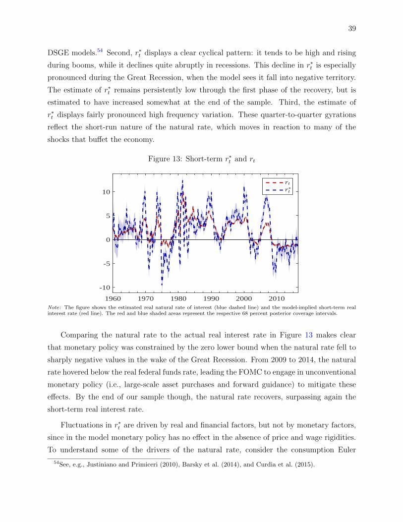
39

DSGE models.54 Second, r∗t displays a clear cyclical pattern: it tends to be high and rising

during booms, while it declines quite abruptly in recessions. This decline in r∗t is especially

pronounced during the Great Recession, when the model sees it fall into negative territory.

The estimate of r∗t remains persistently low through the first phase of the recovery, but is

estimated to have increased somewhat at the end of the sample. Third, the estimate of

r∗t displays fairly pronounced high frequency variation. These quarter-to-quarter gyrations

reflect the short-run nature of the natural rate, which moves in reaction to many of the

shocks that buffet the economy.

Figure 13: Short-term r∗t and rt

1960 1970 1980 1990 2000 2010

-10

-5

0

5

10

rt

r$t

Note: The figure shows the estimated real natural rate of interest (blue dashed line) and the model-implied short-term realinterest rate (red line). The red and blue shaded areas represent the respective 68 percent posterior coverage intervals.

Comparing the natural rate to the actual real interest rate in Figure 13 makes clear

that monetary policy was constrained by the zero lower bound when the natural rate fell to

sharply negative values in the wake of the Great Recession. From 2009 to 2014, the natural

rate hovered below the real federal funds rate, leading the FOMC to engage in unconventional

monetary policy (i.e., large-scale asset purchases and forward guidance) to mitigate these

effects. By the end of our sample though, the natural rate recovers, surpassing again the

short-term real interest rate.

Fluctuations in r∗t are driven by real and financial factors, but not by monetary factors,

since in the model monetary policy has no effect in the absence of price and wage rigidities.

To understand some of the drivers of the natural rate, consider the consumption Euler

54See, e.g., Justiniano and Primiceri (2010), Barsky et al. (2014), and Curdia et al. (2015).

40

equation (25). The same equation holds also in the counterfactual economy in which prices

and wages are fully flexible. Solving that equation for r∗t , we obtain

r∗t = −cyt+σc

1− h(IEt

[c∗t+1 − c∗t + zt+1

]− h

(c∗t − c∗t−1 + zt

))− (σc − 1)

(1− h)

w∗L∗c∗

IEt[L∗t+1−L∗t ],

(26)

where c∗t and L∗t denote respectively the level of consumption and hours worked in the

flexible price economy. This expression reveals that r∗t falls one-for-one with any increase in

the convenience yield cyt. The natural rate also increases with higher expected consumption

growth or lower growth in labor supply in the flexible-price economy.

Figure 14: Short-term r∗t and its Drivers

1960 1970 1980 1990 2000 2010

−10

−5

0

5

10

Convenience Yield Risk Productivity Other

Note: The figure shows the real natural rate implied by the DSGE model (black solid line) in deviations from the steady state.It also shows the contribution of shocks to the convenience yield (in red), risk shocks σω,t (in green), productivity shocks (inblue), and other shocks (in grey) in causing fluctuations in the natural rate.

Figure 14 decomposes the r∗t estimate shown in Figure 13 in terms of the shocks that

account for its movements. As before, the red bars capture exogenous fluctuations in conve-

nience yields cyt; green bars display fluctuations due to risk shocks σω,t, which increase the

cost of external finance for firms, reducing the demand for investment. Productivity shocks

(in blue) also depress desired consumption and investment, and lower the natural rate. The

remaining shocks are in gray.

We draw two main lessons from Figure 14. First, r∗t plunged during the recent financial

crisis and the recession that followed due to an unusual combination of severe financial, risk,

41

and productivity shocks. Second, among these negative contributions, shocks to convenience

yields and negative productivity shocks have had particularly pronounced effects.

IV Conclusion

We estimated the natural rate of interest and its fundamental drivers using two very dif-

ferent methodologies. The first one is a flexible multivariate unobserved component model

estimated using data on Treasury and corporate bond yields of various maturities, inflation,

and survey expectations, which we used to make inference on slow-moving trends in the nat-

ural rate. The second is a medium-scale DSGE model with nominal and financial frictions,

estimated using the same data on yields, along with a large set of other macroeconomic

variables, whose tighter structure allows us to recover the entire time path of the natural

rate.

The two approaches yield remarkably consistent results. First, they both isolate a slow-

moving trend in the real interest rate that is fairly flat between 2 and 2.5 percent until the late

1990s, when it starts declining towards a recent trough at around 1 percent. Second, they

both attribute most of this decline to an increase in the convenience yield on Treasuries,

which they identify as a low-frequency component in the spreads between corporate and

Treasury bonds with the same maturity, but different characteristics in terms of liquidity

and safety. In addition, the DSGE model sees these factors as also playing an important

role in the movements of the natural rate at business cycle frequencies. Finally, the DSGE

model suggests that the short-term interest rate was severely constrained by the effective

lower bound on nominal interest rates starting in late 2008, when the natural rate plunged

well into negative territory.

Going forward, both our models suggest that the natural rate of interest will likely remain

low due to its depressed secular component. Yet, this conclusion is subject to significant

uncertainty, since sudden changes in expectations, regulation, market structure, investors’

degree of risk aversion, or in their perceptions of the safety and liquidity attributes of U.S.

Treasuries could all be sources of shocks to this trend. Although we have identified a rise

in the measured convenience yield as a key driver of the secular decline in the natural rate

of interest, we have not investigated the underlying sources of these changes in the premia

commanded by liquid and safe assets. This is something we leave for future research.

42

References

Acharya, Viral V. and Lasse Heje Pedersen, “Asset pricing with liquidity risk,” Journalof Financial Economics, 2005, 77 (2), 375–410.

Adrian, Tobias and Hyun Song Shin, “Money, Liquidity, and Monetary Policy,” TheAmerican Economic Review, 2009, 99 (2), 600–605.

and , “Financial intermediaries and monetary economics,” in Benjamin M. Friedmanand Michael Woodford, eds., Handbook of Monetary Economics, Vol. 3, Elsevier, 2010.

Ajello, Andrea, “Financial Intermediation, Investment Dynamics and Business Cycle Fluc-tuations,” American Economic Review, forthcoming.

Amihud, Yakov, Haim Mendelson, and Lasse Heje Pedersen, Market liquidity: assetpricing, risk, and crises, Cambridge University Press, 2012.

, , et al., “Liquidity and asset prices,” Foundations and Trends R© in Finance, 2006,1 (4), 269–364.

Anzoategui, Diego, Diego Comin, Mark Gertler, and Joseba Martinez, “Endoge-nous Technology Adoption and R&D as Sources of Business Cycle Persistence,” 2015. NewYork University working paper.

Auclert, Adrien and Matthew Rognlie, “Inequality and Aggregate Demand,” TechnicalReport, Stanford University 2016.

Barsky, Robert, Alejandro Justiniano, and Leonardo Melosi, “The Natural Rate ofInterest and Its Usefulness for Monetary Policy,” American Economic Review, May 2014,104 (5), 37–43.

Basel Committee on Banking Supervision, “Basel III: The Liquidity Coverage Ratioand liquidity risk monitoring tools,” Bank for International Settlements, 2013.

Basu, Susanto, John G Fernald, and Miles S Kimball, “Are technology improvementscontractionary?,” The American Economic Review, 2006, 96 (5), 1418–1448.

Bauer, Michael D, Glenn D Rudebusch, and Jing Cynthia Wu, “Correcting estima-tion bias in dynamic term structure models,” Journal of Business & Economic Statistics,2012, 30 (3), 454–467.

, , and , “Term premia and inflation uncertainty: empirical evidence from an in-ternational panel dataset: comment,” The American Economic Review, 2014, 104 (1),323–337.

Benigno, Gianluca and Luca Fornaro, “Stagnation traps,” Mimeo, LSE and UPF, 2016.

Bernanke, Ben, Mark Gertler, and Simon Gilchrist, “The Financial Accelerator in aQuantitative Business Cycle Framework,” in John B. Taylor and Michael Woodford, eds.,Handbook of Macroeconomics, Vol. 1C, North Holland, Amsterdam, 1999.

Bernanke, Ben S., “The global saving glut and the U.S. current account deficit,” 2005.

, Carol C. Bertaut, Laurie DeMarco, and Steven B. Kamin, “International capitalflows and the return to safe assets in the united states, 2003-2007,” Board of Governorsof the Federal Reserve System International Finance Discussion Papers 1014, 2011.

, Mark Gertler, and Simon Gilchrist, “The Financial Accelerator in a QuantitativeBusiness Cycle Framework,” in John B. Taylor and Michael Woodford, eds., Handbook ofMacroeconomics, Vol. 1C, Amsterdam: North-Holland, 1999, chapter 21, pp. 1341–93.

43

Bigio, Saki, “Endogenous Liquidity and the Business Cycle,” American Economic Review,2015, 105 (6), 1883–1927.

Blanchard, Olivier and Jordi Galı, “Real Wage Rigidities and the New KeynesianModel,” Journal of Money, Credit and Banking, 02 2007, 39 (s1), 35–65.

Bloom, Nicholas, “The impact of uncertainty shocks,” Econometrica, 2009, 77 (3), 623–685.

Boivin, Jean and Marc P. Giannoni, “DSGE Models in a Data Rich Enviroment,”NBER Working Paper, 2006, 12772.

Caballero, Ricardo J., “The “other” imbalance and the financial crisis,” National Bureauof Economic Research WP 15636, 2010.

Caballero, Ricardo J and Arvind Krishnamurthy, “Global imbalances and financialfragility,” National Bureau of Economic Research WP 14688, 2009.

Caballero, Ricardo J. and Emmanuel Farhi, “The safety trap,” National Bureau ofEconomic Research WP 19927, 2014.

, , and Pierre-Olivier Gourinchas, “Global Imbalances and Currency Wars at theZLB,” National Bureau of Economic Research WP 21670, 2015.

Carter, C.K. and Robert Kohn, “On Gibbs Sampling for State Space Models,”Biometrika, 1994, 81 (3), 541–553.

Carvalho, Carlos, Andrea Ferrero, and Fernanda Nechio, “Demographics and realinterest rates: Inspecting the mechanism,” European Economic Review, 2016, pp. –.

Christensen, Jens H. E. and Glenn D. Rudebusch, “A New Normal for Interest Rates?Evidence from Inflation-Indexed Debt,” Mimeo, Federal Reserve Bank of San Franciscoworking paper, 2016.

Christiano, Lawrence J., Martin Eichenbaum, and Charles L. Evans, “NominalRigidities and the Dynamic Effects of a Shock to Monetary Policy,” Journal of PoliticalEconomy, 2005, 113, 1–45.

, Roberto Motto, and Massimo Rostagno, “The Great Depression and the Friedman-Schwartz Hypothesis,” Journal of Money, Credit and Banking, 2003, 35, 1119–1197.

, , and , “Risk Shocks,” American Economic Review, 2014, 104 (1), 27–65.

Cieslak, Anna and Pavol Povala, “Expected Returns in Treasury Bonds,” Review ofFinancial Studies, 2015, 28 (10), 2859–2901.

Clark, Todd E and Taeyoung Doh, “Evaluating alternative models of trend inflation,”International Journal of Forecasting, 2014, 30 (3), 426–448.

Comin, Diego and Mark Gertler, “Medium-Term Business Cycles,” American EconomicReview, June 2006, 96 (3), 523–551.

Crump, Richard K, Stefano Eusepi, and Emanuel Moench, “The term structure ofexpectations and bond yields,” Federal Reserve Bank of New YorkStaff Report No. 775,2016.

Cui, Wei and Soren Radde, “Search-Based Endogenous Illiquidity and the Macroecon-omy,” Available at SSRN 2432935, 2014.

44

Curdia, Vasco, Andrea Ferrero, Ging Cee Ng, and Andrea Tambalotti, “Has U.S.Monetary Policy Tracked the Efficient Interest Rate?,” Journal of Monetary Economics,2015, 70 (C), 72–83.

De Graeve, Ferre, “The External Finance Premium and the Macroeconomy: US Post-WWII Evidence,” Journal of Economic Dynamics and Control, 2008, 32 (11), 3415 –3440.

Del Negro, Marco and Giorgio E Primiceri, “Time varying structural vector autore-gressions and monetary policy: a corrigendum,” The review of economic studies, 2015, 82(4), 1342–1345.

, Gauti Eggertsson, Andrea Ferrero, and Nobuhiro Kiyotaki, “The Great Escape?A Quantitative Evaluation of the Feds Liquidity Facilities,” American Economic Review,2017.

, Marc P Giannoni, and Frank Schorfheide, “Inflation in the Great Recession andNew Keynesian Models,” American Economic Journal: Macroeconomics, 2015, 7 (1), 168–196.

Durbin, James and Siem Jan Koopman, “A Simple and Efficient Simulation Smootherfor State Space Time Series Analysis,” Biometrika, 2002, 89 (3), 603–616.

Edge, Rochelle M., Michael T. Riley, and Jean-Philippe Laforte, “Natural ratemeasures in an estimated DSGE model of the U.S. economy,” Journal of Economic Dy-namics and Control, 2008, 32 (8), 2512 – 2535.

Eggertsson, Gauti B. and Neil R. Mehrotra, “A Model of Secular Stagnation,” NBERWorking Papers 20574, National Bureau of Economic Research, Inc October 2014.

Eichengreen, Barry, “Secular Stagnation: The Long View,” American Economic Review,May 2015, 105 (5), 66–70.

Favero, Carlo A., Arie E. Gozluklu, and Haoxi Yang, “Demographics and the Be-havior of Interest Rates,” IMF Economic Review, November 2016, 64 (4), 732–776.

Fisher, Jonas, “On the Structural Interpretation of the Smets–Wouters Risk Premium?Shock,” Journal of Money, Credit and Banking, 2015, 47 (2-3), 511–516.

Fleckenstein, Matthias, Francis A Longstaff, and Hanno Lustig, “The TIPS-Treasury Bond Puzzle,” The Journal of Finance, 2014, 69 (5), 2151–2197.

Gagnon, Etienne, Benjamin K. Johannsen, and J. David Lopez-Salido, “Under-standing the New Normal : The Role of Demographics,” Finance and Economics Discus-sion Series 2016-080, Board of Governors of the Federal Reserve System (U.S.) September2016.

Garleanu, Nicolae and Lasse Heje Pedersen, “Margin-Based Asset Pricing and Devi-ations from the Law of One Price,” Review of Financial Studies, 2011, 24 (6), 1980–2022.

Giannone, Domenico, Michele Lenza, and Giorgio E Primiceri, “Prior selection forvector autoregressions,” Review of Economics and Statistics, 2015, 97 (2), 436–451.

Gilchrist, Simon and Egon Zakrajsek, “Credit Spreads and Business Cycle Fluctua-tions,” American Economic Review, 2012, 102 (4), 1692–1720.

Gorton, Gary and Andrew Metrick, “Securitized banking and the run on repo,” Journalof Financial economics, 2012, 104 (3), 425–451.

45

Gorton, Gary B., “The History and Economics of Safe Assets,” National Bureau of Eco-nomic Research WP 22210, 2016.

Gourinchas, Pierre-Olivier and Helene Rey, “Real Interest Rates, Imbalances and theCurse of Regional Safe Asset Providers at the Zero Lower Bound,” National Bureau ofEconomic Research WP 22618, 2016.

Greenwood, Jeremy, Zvi Hercowitz, and Per Krusell, “Long-Run Implications ofInvestment-Specific Technological Change,” American Economic Review, 1998, 87 (3),342–36.

Greenwood, Robin, Samuel G Hanson, and Jeremy C Stein, “A Comparative-Advantage Approach to Government Debt Maturity,” The Journal of Finance, 2015, 70(4), 1683–1722.

, , and , “The Federal Reserves balance sheet as a financial-stability tool,” in ““De-signing Resilient Monetary Policy Frameworks for the Future,” Jackson Hole Symposium:Federal Reserve Bank of Kansas City” 2016.

Guerron-Quintana, Pablo and Ryo Jinnai, “Liquidity Shocks and Asset Prices,” 2015.Working Paper, Federal Reserve Bank of Philadelphia.

Hall, Robert E, “Understanding the decline in the safe real interest rate,” National Bureauof Economic Research WP 22196, 2016.

Hamilton, James D., Ethan S. Harris, Jan Hatzius, and Kenneth D. West, “TheEquilibrium Real Funds Rate: Past, Present and Future,” NBER Working Papers 21476,National Bureau of Economic Research, Inc August 2015.

Hansen, Alvin H., “Economic Progress and Declining Population Growth,” The AmericanEconomic Review, 1939, 29 (1), 1–15.

Johannsen, Benjamin K. and Elmar Mertens, “A Time Series Model of Interest RatesWith the Effective Lower Bound,” Finance and Economics Discussion Series 2016-033,Board of Governors of the Federal Reserve System April 2016.

Justiniano, Alejandro and Giorgio E. Primiceri, “Measuring the equilibrium realinterest rate,” Economic Perspectives, 2010, (Q I), 14–27.

, Giogrio Primiceri, and Andrea Tambalotti, “Investment Shocks and BusinessSycles,” Journal of Monetary Economics, 2010, 57 (2), 132–145.

, Giorgio E. Primiceri, and Andrea Tambalotti, “Is There a Trade-Off between In-flation and Output Stabilization?,” American Economic Journal: Macroeconomics, April2013, 5 (2), 1–31.

Kiley, Michael T., “What Can the Data Tell Us About the Equilibrium Real InterestRate?,” Finance and Economics Discussion Series 2015-77, Board of Governors of theFederal Reserve System August 2015.

and John M. Roberts, “Monetary Policy in a Low Interest-Rate World,” BrookingsPapers on Economic Activity, this issue.

Kiyotaki, Nobuhiro and John Moore, “Liquidity, Business Cycles, and Monetary Pol-icy,” NBER Working Paper No. 17934, 2012.

Kozicki, Sharon and Peter A Tinsley, “Effective use of survey information in estimatingthe evolution of expected inflation,” Journal of Money, Credit and Banking, 2012, 44 (1),145–169.

46

Krishnamurthy, Arvind and Annette Vissing-Jorgensen, “The Aggregate Demandfor Treasury Debt,” Journal of Political Economy, 2012, 120 (2), 233 – 267.

Kurlat, Pablo, “Lemons Markets and the Transmission of Aggregate Shocks,” AmericanEconomic Review, 2013, 103 (4), 1463–1489.

Laseen, Stefan and Lars E.O. Svensson, “Anticipated Alternative Policy-Rate Paths inPolicy Simulations,” International Journal of Central Banking, 2011, 7 (3), 1–35.

Laubach, Thomas and John C. Williams, “Measuring the Natural Rate of Interest,”The Review of Economics and Statistics, November 2003, 85 (4), 1063–1070.

and John C Williams, “Measuring the Natural Rate of Interest Redux,” BusinessEconomics, 2016, 51 (2), 57–67.

Longstaff, Francis, Sanjay Mithal, and Eric Neis, “The Flight-to-Liquidity Premiumin U.S. Treasury Bond Prices,” Journal of Business, 2004, 77 (3), 511–526.

, , and , “Corporate Yield Spreads: Default Risk or Liquidity? New Evidence fromthe Credit Default Swap Market,” Journal of Finance, 2005, 60 (5), 2213–2253.

Lopez-Salido, David, Jeremy C Stein, and Egon Zakrajsek, “Credit-market senti-ment and the business cycle,” National Bureau of Economic Research WP 21879, 2016.

Lubik, Thomas A, Christian Matthes et al., “Calculating the natural rate of interest:A comparison of two alternative approaches,” Richmond Fed Economic Brief, 2015, (Oct),1–6.

Neiss, Katharine S. and Edward Nelson, “The Real-Interest-Rate Gap As An InflationIndicator,” Macroeconomic Dynamics, April 2003, 7 (02), 239–262.

Pescatori, Andrea and Jarkko Turunen, “Lower for Longer; Neutral Rates in the UnitedStates,” IMF Working Papers 15/135, International Monetary Fund June 2015.

Rachel, Lukasz and Thomas Smith, “Secular Drivers of the Global Real Interest Rate,”Discussion Papers 1605, Centre for Macroeconomics (CFM) December 2015.

Sims, Christopher A. and Tao Zha, “Bayesian Methods for Dynamic Multivariate Mod-els,” International Economic Review, 1998, 39 (4), 949–968.

Smets, Frank and Raf Wouters, “Shocks and Frictions in US Business Cycles: ABayesian DSGE Approach,” American Economic Review, 2007, 97 (3), 586 – 606.

Stock, James H and Mark W Watson, “Testing for common trends,” Journal of theAmerican statistical Association, 1988, 83 (404), 1097–1107.

Stock, James H. and Mark W. Watson, “Median Unbiased Estimation of CoefficientVariance in a Time-Varying Parameter Model,” Journal of the American Statistical Asso-ciation, August 1998, (441), 349–358.

and , “Forecasting Inflation,” Journal of Monetary Economics, 1999, 44 (2), 293–335.

Stock, James H and Mark W Watson, “Why has US inflation become harder to fore-cast?,” Journal of Money, Credit and banking, 2007, 39 (s1), 3–33.

Summers, Lawrence H., Secular Stagnation: Facts, Causes and Cures, CEPR Press,

Villani, Mattias, “Steady State Priors for Vector Autoregressions,” Journal of AppliedEconometrics, 2009, 24 (4), 630–650.

47

Vissing-Jorgensen, Annette, “Limited Asset Market Participation and the Elasticity ofIntertemporal Substitution,” Journal of Political Economy, 2002, 110 (4), 825–853.

Watson, Mark W, “Univariate detrending methods with stochastic trends,” Journal ofmonetary economics, 1986, 18 (1), 49–75.

Wicksell, Knut, Interest and Prices, english translation by r.f. kahn, 1936 ed., McMillan,London, 1898.

Woodford, Michael, Interest and Prices: Foundations of a Theory of Monetary Policy,Princeton University Press, 2003.

Wright, Jonathan H, “Term premia and inflation uncertainty: Empirical evidence from aninternational panel dataset,” The American Economic Review, 2011, 101 (4), 1514–1534.

Wu, Jing Cynthia and Ji Zhang, “A Shadow Rate New Keynesian Model,” NationalBureau of Economic Research WP 22856, 2016.

Yellen, Janet, “The Economic Outlook and Monetary Policy,” December 2 2015.

Appendix not intended for publication A-1

Online Appendix for

“Safety, Liquidity, and the Natural Rate of Interest”

Marco Del Negro, Domenico Giannone, Marc Giannoni, Andrea Tambalotti

A Gibbs Sampler for VARs with Common Trends

Let use the notation xi:j to denote the sequence xi, .., xj for a generic variable xt. The

Gibbs sampler is structured according to the following blocks:

1. y0:T , y−p+1:T , λ|ϕ,Σε,Σe, y1:T

(a) λ|ϕ,Σε,Σe, y1:T

(b) y0:T , y−p+1:T |λ, ϕ,Σε,Σe, y1:T

2. ϕ,Σε,Σe|y0:T , y−p+1:T , λ, y1:T

(a) Σε,Σe|y0:T , y−p+1:T , λ, y1:T

(b) ϕ|Σε,Σe, y0:T , y−p+1:T , λ, y1:T

Details of each step follow:

1. y0:T , y−p+1:T , λ|ϕ,Σε,Σe, y1:T

This is given by the product of the marginal posterior distribution of λ (conditional

on the other parameters) times the distribution of y0:T , y−p+1:T conditional on λ (and

the other parameters).

(a) λ|ϕ,Σε,Σe, y1:T

The marginal posterior distribution of λ (conditional on the other parameters) is

given by

p(λ|ϕ,Σε,Σe, y1:T ) ∝ L(y1:T |λ, ϕ,Σε,Σe)p(λ),

where L(y1:T |λ, ϕ,Σε,Σe) is the likelihood obtained from the Kalman filter applied

to the state space system (2) through (6). p(λ|ϕ,Σε,Σe, y1:T ) does not have a

known form so we will use a Metropolis Hastings step.

Appendix not intended for publication A-2

(b) y0:T , y−p+1:T |λ, ϕ,Σε,Σe, y1:T

Given λ and the other parameters of the state space model we can use Durbin

and Koopman (2002)’s simulation smoother to obtain draws for the latent states

y0:T and y−p+1:T . Note that in addition to y1:T and y1:T we also need to draw the

initial conditions y0 and y−p+1:0 in order to estimate the parameters of (4) and

(3) in the next Gibbs sampler step.

Note that missing observations do not present any difficulty in terms of carrying out

this step: if the vector yt0 has some missing elements, the corresponding rows of the

observation equation (2) are simply deleted for t = t0.

2. ϕ,Σε,Σe|y0:T , y−p+1:T , λ, y1:T

This step is straightforward because for given y0:T and y−p+1:T equations (3) and (4)

are standard VARs where in case of (3) we actually know the autoregressive matrices.

The posterior distribution of Σe is given by

p(Σe|y0:T ) = IW(Σe + Se, κe + T )

where Se =T∑t=1

(yt − yt−1)(yt − yt−1)′. The posterior distribution of ϕ and Σε is given

by

p(Σε|y0:T ) = IW(Σε + Sε, κε + T ),

p(ϕ|Σε, y0:T ) = N

vec(Φ),Σε ⊗

(T∑t=1

xtx′t + Ω−1

)−1 ,

where xt = (y′t−1, .., y′t−p)

′ collects the VAR regressors,

Φ =

(T∑t=1

xtx′t + Ω−1

)−1( T∑t=1

xty′t + Ω−1Φ

), Sε =

T∑t=1

εtε′t+(Φ−Φ)′Ω−1(Φ−Φ),

and εt = yt − Φ′xt are the VAR residuals.

We use 100,000 draws and discard the first 50,000.

Appendix not intended for publication A-3

B DSGE model

This section describes the model specification, the data used, how they relate to the model

concepts, and the priors distributions assumed for estimation.

The model economy is populated by eight classes of agents: 1) a continuum of house-

holds, who consume and supply differentiated labor; 2) competitive labor aggregators that

combine labor supplied by individual households; 3) competitive final good-producing firms

that aggregate the intermediate goods into a final product; 4) a continuum of monopo-

listically competitive intermediate good producing firms; 5) competitive capital producers

that convert final goods into capital; 6) a continuum of entrepreneurs who purchase capital

using both internal and borrowed funds and rent it to intermediate good producing firms;

7) a representative bank collecting deposits from the households and lending funds to the

entrepreneurs; and finally 8) a government, composed of a monetary authority that sets

short-term interest rates and a fiscal authority that sets public spending and collects taxes.

We solve each agent’s problem, and derive the resulting equilibrium conditions, which we

approximate around the non-stochastic steady state. Since the derivation follows closely the

literature (e.g., Christiano et al. (2005)), we describe here the log-linearized conditions.

Growth in the economy is driven by technological progress, Z∗t = e1

1−α ztZpt eγt, which is

assumed to include a deterministic trend (eγt), a stochastic trend (Zpt ), and a stationary

component (zt), where α is the income share of capital (after paying mark-ups and fixed

costs in production). Trending variables are divided by Z∗t to express the model’s equilibrium

conditions in terms of the stationary variables. In what follows, all variables are expressed in

log deviations from their steady state, and steady-state values are denoted by ∗-subscripts.

The stationary component of productivity zt and the growth rate of the stochastic trend

zpt = log(Zpt /Z

pt−1) are assumed to follow AR(1) processes:

zt = ρz zt−1 + σzεz,t, εz,t ∼ N(0, 1). (A-1)

zpt = ρzpzpt−1 + σzpεzp,t, εzp,t ∼ N(0, 1). (A-2)

The growth rate of technology evolves thus according to

zt ≡ log(Z∗t /Z∗t−1)− γ =

1

1− α(ρz − 1)zt−1 +

1

1− ασzεz,t + zpt , (A-3)

where γ is the steady-state growth rate of the economy.

Appendix not intended for publication A-4

The optimal allocation of consumption satisfies the following Euler equation:

ct = − 1− hσc(1 + h)

(Rt − IEt[πt+1] + cyt) +h

1 + h(ct−1 − zt)

+1

1 + hIEt [ct+1 + zt+1] +

(σc − 1)

σc(1 + h)

w∗L∗c∗

(Lt − IEt[Lt+1]) , (A-4)

where ct is consumption, Lt denotes hours worked, Rt is the nominal interest rate, and πt

is inflation. The parameter σc captures the degree of relative risk aversion while h ≡ he−γ

depends on the degree of habit persistence in consumption, h, and steady-state growth. This

equation includes hours worked because utility is non-separable in consumption and leisure.

The convenience yield cyt contains both a liquidity component cylt and a safety component

cylt

cyt = cylt + cylt, (A-5)

where we let each premium be given by the sum of two AR(1) processes, one that captures

transitory fluctuations, and one that captures highly persistent movements.

The optimal investment decision satisfies the following relationship between the level of

investment it, measured in terms of consumption goods, and the value of capital in terms of

consumption qkt :

it =qkt

S ′′e2γ(1 + β)+

1

1 + β(it−1 − zt) +

β

1 + βIEt [it+1 + zt+1] + µt. (A-6)

This relationship shows that investment is affected by investment adjustment costs (S ′′ is the

second derivative of the adjustment cost function) and by an exogenous process µt, which

we call “marginal efficiency of investment”, that alters the rate of transformation between

consumption and installed capital (see Greenwood et al. (1998)). The shock µt follows an

AR(1) process with parameters ρµ and σµ. The parameter β ≡ βe(1−σc)γ depends on the

intertemporal discount rate in the household utility function, β, on the degree of relative

risk aversion σc, and on the steady-state growth rate γ.

The capital stock, kt, which we refer to as “installed capital”, evolves as

kt =

(1− i∗

k∗

)(kt−1 − zt

)+i∗k∗it +

i∗k∗S′′e2γ(1 + β)µt, (A-7)

where i∗/k∗ is the steady state investment to capital ratio. Capital is subject to variable

capacity utilization ut; effective capital rented out to firms, kt, is related to kt by:

kt = ut − zt + kt−1. (A-8)

Appendix not intended for publication A-5

The optimality condition determining the rate of capital utilization is given by

1− ψψ

rkt = ut, (A-9)

where rkt is the rental rate of capital and ψ captures the utilization costs in terms of foregone

consumption.

Real marginal costs for firms are given by

mct = wt + αLt − αkt, (A-10)

where wt is the real wage. From the optimality conditions of goods producers it follows that

all firms have the same capital-labor ratio:

kt = wt − rkt + Lt. (A-11)

We include financial frictions in the model, building on the work of Bernanke et al.

(1999), Christiano et al. (2003), De Graeve (2008), and Christiano et al. (2014). We assume

that banks collect deposits from households and lend to entrepreneurs who use these funds

as well as their own wealth to acquire physical capital, which is rented to intermediate goods

producers. Entrepreneurs are subject to idiosyncratic disturbances that affect their ability

to manage capital. Their revenue may thus turn out to be too low to pay back the loans

received by the banks. The banks therefore protect themselves against default risk by pooling

all loans and charging a spread over the deposit rate. This spread may vary as a function of

entrepreneurs’ leverage and riskiness.

The realized return on capital is given by

Rkt − πt =

rk∗rk∗ + (1− δ)

rkt +(1− δ)

rk∗ + (1− δ)qkt − qkt−1, (A-12)

where Rkt is the gross nominal return on capital for entrepreneurs, rk∗ is the steady state

value of the rental rate of capital rkt , and δ is the depreciation rate.

The excess return on capital (the spread between the expected return on capital and the

riskless rate) can be expressed as a function of the convenience yield cyt, the entrepreneurs’

leverage (i.e. the ratio of the value of capital to net worth), and “risk shocks” σω,t capturing

mean-preserving changes in the cross-sectional dispersion of ability across entrepreneurs (see

Christiano et al. (2014)):

Et

[Rkt+1 −Rt

]= cyt + ζsp,b

(qkt + kt − nt

)+ σω,t, (A-13)

Appendix not intended for publication A-6

where nt is entrepreneurs’ net worth, ζsp,b is the elasticity of the credit spread to the en-

trepreneurs’ leverage (qkt + kt − nt). σω,t follows an AR(1) process with parameters ρσω and

σσω . Entrepreneurs’ net worth nt evolves in turn according to

nt = ζn,Rk(Rkt − πt

)− ζn,R (Rt−1 − πt + cyt−1) + ζn,qK

(qkt−1 + kt−1

)+ ζn,nnt−1

−γ∗v∗n∗zt −

ζn,σωζsp,σω

σω,t−1,(A-14)

where the ζ’s denote elasticities, that depend among others on the entrepreneurs’ steady-

state default probability F (ω), where γ∗ is the fraction of entrepreneurs that survive and

continue operating for another period, and where v∗ is the entrepreneurs’ real equity divided

by Z∗t , in steady state.

The production function is

yt = Φp (αkt + (1− α)Lt) , (A-15)

where Φp = 1 + Φ/y∗, and Φ measures the size of fixed costs in production. The resource

constraint is:

yt = g∗gt +c∗y∗ct +

i∗y∗it +

rk∗k∗y∗

ut. (A-16)

where gt = log(Gt

Z∗t y∗g∗) and g∗ = 1− c∗ + i∗

y∗. Government spending gt is assumed to follow

the exogenous process:

gt = ρggt−1 + σgεg,t + ηgzσzεz,t.

Optimal decisions for price and wage setting deliver the price and wage Phillips curves,

which are respectively:

πt = κ mct +ιp

1 + ιpβπt−1 +

β

1 + ιpβIEt[πt+1] + λf,t, (A-17)

and

wt =(1− ζwβ)(1− ζw)

(1 + β)ζw((λw − 1)εw + 1)

(wht − wt

)− 1 + ιwβ

1 + βπt +

1

1 + β(wt−1 − zt + ιwπt−1)

+β

1 + βIEt [wt+1 + zt+1 + πt+1] + λw,t, (A-18)

where κ =(1− ζpβ)(1− ζp)

(1 + ιpβ)ζp((Φp − 1)εp + 1), the parameters ζp, ιp, and εp are the Calvo parameter,

the degree of indexation, and the curvature parameter in the Kimball aggregator for prices,

Appendix not intended for publication A-7

and ζw, ιw, and εw are the corresponding parameters for wages. wht measures the household’s

marginal rate of substitution between consumption and labor, and is given by:

wht =1

1− h(ct − hct−1 + hzt

)+ νlLt, (A-19)

where νl characterizes the curvature of the disutility of labor (and would equal the inverse

of the Frisch elasticity in the absence of wage rigidities). The mark-ups λf,t and λw,t follow

the exogenous ARMA(1,1) processes:

λf,t = ρλfλf,t−1 + σλf ελf ,t − ηλfσλf ελf ,t−1,

and

λw,t = ρλwλw,t−1 + σλwελw,t − ηλwσλwελw,t−1.

Finally, the monetary authority follows a policy feedback rule:

Rt = ρRRt−1 + (1− ρR) (ψ1(πt − π∗t ) + ψ2(yt − y∗t )) (A-20)

+ψ3

((yt − y∗t )− (yt−1 − y∗t−1)

)+ rmt .

where π∗t is a time-varying inflation target, y∗t is a measure of the “full-employment level of

output,” and rmt captures exogenous departures from the policy rule.

The time-varying inflation target π∗t is meant to capture the rise and fall of inflation

and interest rates in the estimation sample.1 As in Aruoba and Schorfheide (2008) and Del

Negro and Eusepi (2011), we use data on long-run inflation expectations in the estimation of

the model. This allows us to pin down the target inflation rate to the extent that long-run

inflation expectations contain information about the central bank’s objective. The time-

varying inflation target evolves according to

π∗t = ρπ∗π∗t−1 + σπ∗επ∗,t, (A-21)

where 0 < ρπ∗ < 1 and επ∗,t is an iid shock. We model π∗t as a stationary process, although

our prior for ρπ∗ will force this process to be highly persistent.

The “full-employment level of output” y∗t represents the level of output that would obtain

if prices and wages were fully flexible and if there were no markup shocks. This variable

along with the natural rate of interest r∗t are obtained by solving the model without nominal

1The assumption that the inflation target moves exogenously is of course a simplification. A more

realistic model would for instance relate movements in trend inflation to the evolution of the policy makers’

understanding of the output-inflation trade-of, as in Sargent (1999) or Primiceri (2006).

Appendix not intended for publication A-8

rigidities and markup shocks (that is, equations (A-4) through (A-19) with ζp = ζw = 0, and

λf,t = λw,t = 0).

The exogenous component of the policy rule rmt evolves according to the following process

rmt = ρrmrmt−1 + εRt +

K∑k=1

εRk,t−k, (A-22)

where εRt is the usual contemporaneous policy shock, and εRk,t−k is a policy shock that is

known to agents at time t − k, but affects the policy rule k periods later, that is, at time

t. We assume that εRk,t−k ∼ N(0, σ2k,r), i.i.d. As argued in Laseen and Svensson (2011), such

anticipated policy shocks allow us to capture the effects of the zero lower bound on nominal

interest rates, as well as the effects of forward guidance in monetary policy.

B.1 State Space Representation and Data

We use the method in Sims (2002) to solve the system of log-linear approximate equilibrium

conditions and obtain the transition equation, which summarizes the evolution of the vector

of state variables st:

st = T (θ)st−1 +R(θ)εt. (A-23)

where θ is a vector collecting all the DSGE model parameters and εt is a vector of all

structural shocks. The state-space representation of our model is composed of the transition

equation (A-23), and a system of measurement equations:

Yt = D(θ) + Z(θ)st, (A-24)

mapping the states into the observable variables Yt, which we describe in detail next.

The estimation of the model is based on data on real output growth (including both

GDP and GDI measures), consumption growth, investment growth, real wage growth, hours

worked, inflation (measured by core PCE and GDP deflators), short- and long- term interest

rates, 10-year inflation expectations, market expectations for the federal funds rate up to

6 quarters ahead, Aaa and Baa credit spreads, and total factor productivity. Measurement

Appendix not intended for publication A-9

equations (A-24) relate these observables to the model variables as follows:

GDP growth = 100γ + (yt − yt−1 + zt) + egdpt − egdpt−1

GDI growth = 100γ + (yt − yt−1 + zt) + egdit − egdit−1

Consumption growth = 100γ + (ct − ct−1 + zt)

Investment growth = 100γ + (it − it−1 + zt)

Real Wage growth = 100γ + (wt − wt−1 + zt)

Hours = L+ Lt

Core PCE Inflation = π∗ + πt + epcet

GDP Deflator Inflation = π∗ + δgdpdef + γgdpdef ∗ πt + egdpdeft

FFR = R∗ +Rt

FFRet,t+j = R∗ + IEt [Rt+j] , j = 1, ..., 6

10y Nominal Bond Yield = R∗ + IEt

[1

40

39∑j=0

Rt+j

]+ e10y

t

10y Infl. Expectations = π∗ + IEt

[1

40

39∑j=0

πt+j

]

Aaa - 20-year Treasury Spread = cyl∗ + IEt

[1

80

79∑j=0

cylt+j

]+ eAaat

Baa - 20-year Treasury Spread = cyl∗ + cys∗ + SP∗ + IEt1

80

79∑j=0

[Rkt+j+1 −Rt+j

]+ eBaat

TFP growth, demeaned = zt +α

1− α(ut − ut−1) + etfpt .

(A-25)

All variables are measured in percent. The terms π∗ and R∗ measure respectively the net

steady-state inflation rate and short-term nominal interest rate, expressed in percentage

terms, and L captures the mean of hours (this variable is measured as an index). We assume

that some of the variables are measured with “error,” that is, the observed value equals

the model implied value plus an AR(1) exogenous process e∗t that can be thought of either

measurement errors or some other unmodeled source of discrepancy between the model and

the data, as in Boivin and Giannoni (2006). For instance, the terms egdpt and egdit capture

measurement error of total output.2 Alternatively, or the long-term nominal interest rate,

2We introduce correlation in the measurement errors for GDP and GDI, which evolve as follows:

egdpt = ρgdp · egdpt−1 + σgdpεgdpt , εgdpt ∼ i.i.d.N(0, 1)

egdit = ρgdi · egdit−1 + %gdp · σgdpεgdpt + σgdiεgdit , εgdit ∼ i.i.d.N(0, 1).

The measurement errors for GDP and GDI are thus stationary in levels, and enter the observation equation

in first differences (e.g. egdpt − egdpt−1 and egdpt − egdpt−1). GDP and GDI are also cointegrated as they are driven

Appendix not intended for publication A-10

the term e10yt captures fluctuations in term premia not captured by the model.

The 10-year inflation expectations contain information about low-frequency movements

of inflation and are obtained from the Blue Chip Economic Indicators survey and the Survey

of Professional Forecasters.

B.2 Inference, Prior and Posterior Parameter Estimates

We estimate the model using Bayesian techniques. This requires the specification of a

prior distribution for the model parameters. For most parameters common with Smets

and Wouters (2007), we use the same marginal prior distributions. As an exception, we

favor a looser prior than Smets and Wouters (2007) for the quarterly steady state inflation

rate π∗; it is centered at 0.75% and has a standard deviation of 0.4%. Regarding the fi-

nancial frictions, we specify priors for the parameters SP∗, ζsp,b, ρσω , and σσω , while we fix

the parameters corresponding to the steady state default probability and the survival rate

of entrepreneurs, respectively. In turn, these parameters imply values for the parameters

of (A-14). Information on the priors and posterior mean is provided in Table A2.

B.3 Data Construction

Data on real GDP (GDPC), the GDP deflator (GDPDEF), core PCE inflation (PCEPILFE),

nominal personal consumption expenditures (PCEC), and nominal fixed private investment

(FPI) are produced at a quarterly frequency by the Bureau of Economic Analysis, and are

included in the National Income and Product Accounts (NIPA). Average weekly hours of

production and nonsupervisory employees for total private industries (AWHNONAG), civil-

ian employment (CE16OV), and the civilian non-institutional population (CNP16OV) are

produced by the Bureau of Labor Statistics (BLS) at a monthly frequency. The first of these

series is obtained from the Establishment Survey, and the remaining from the Household

Survey. Both surveys are released in the BLS Employment Situation Summary. Since our

models are estimated on quarterly data, we take averages of the monthly data. Compen-

sation per hour for the non-farm business sector (COMPNFB) is obtained from the Labor

Productvity and Costs release, and produced by the BLS at a quarterly frequency. The

data are transformed following Smets and Wouters (2007), with the exception of the civilian

population data, which are filtered using the Hodrick-Prescott filter to remove jumps around

by a comment stochastic trend.

Appendix not intended for publication A-11

census dates. The federal funds rate is obtained from the Federal Reserve Board’s H.15 re-

lease at a business day frequency. We take quarterly averages of the annualized daily data

and divide by four. Let ∆ denote the temporal difference operator. Then:

Output growth = 100 ∗∆LN((GDPC)/CNP16OV )

Consumption growth = 100 ∗∆LN((PCEC/GDPDEF )/CNP16OV )

Investment growth = 100 ∗∆LN((FPI/GDPDEF )/CNP16OV )

Real wage growth = 100 ∗∆LN(COMPNFB/GDPDEF )

Hours worked = 100 ∗ LN((AWHNONAG ∗ CE16OV/100)/CNP16OV )

GDP Deflator Inflation = 100 ∗∆LN(GDPDEF )

Core PCE Inflation = 100 ∗∆LN(PCEPILFE)

FFR = (1/4) ∗ FEDERAL FUNDS RATE

Long-run inflation expectations are obtained from the Blue Chip Economic Indicators

survey and the Survey of Professional Forecasters available from the FRB Philadelphia’s

Real-Time Data Research Center. Long-run inflation expectations (average CPI inflation

over the next 10 years) are available from 1991Q4 onward. Prior to 1991Q4, we use the

10-year expectations data from the Blue Chip survey to construct a long time series that

begins in 1979Q4. Since the Blue Chip survey reports long-run inflation expectations only

twice a year, we treat these expectations in the remaining quarters as missing observations

and adjust the measurement equation of the Kalman filter accordingly. Long-run inflation

expectations πO,40t are therefore measured as

10y Infl Exp = (10-year average CPI inflation forecast− 0.50)/4.

where 0.50 is the average difference between CPI and GDP annualized inflation from the

beginning of the sample to 1992. We divide by 4 to express the data in quarterly terms.

We measure Spread as the annualized Moody’s Seasoned Baa Corporate Bond Yield

spread over the 10-Year Treasury Note Yield at Constant Maturity. Both series are available

from the Federal Reserve Board’s H.15 release. Like the federal funds rate, the spread data

are also averaged over each quarter and measured at a quarterly frequency. This leads to:

Spread = (1/4) ∗ (Baa Corporate − 10 year Treasury).

Similarly,

10y Bond yield = (1/4) ∗ (10 year Treasury).

Appendix not intended for publication A-12

Lastly, TFP growth is measured using John Fernald’s TFP growth series, unadjusted

for changes in utilization. That series is demeaned, divided by 4 to express it in quarterly

growth rates, and divided by Fernald’s estimate of (1−α) to convert it in labor augmenting

terms:

TFP growth, demeaned = (1/4)∗(Fernald’s TFP growth, unadjusted, demeaned) /(1− α).

Appendix not intended for publication A-13

C Additional Tables and Figures – VARs (Section II)

Figure A1: Other Trends and Observables, Baseline Model

tpt and R80,t −R1,t

Q1-60 Q1-70 Q1-80 Q1-90 Q1-00 Q1-10

-1

0

1

2

3

4

Note: The figure shows R80,t −R1,t (dotted blue line) together with the trend tpt. For the trend, the dashed black line showsthe posterior median and the shaded areas show the 68 and 95 percent posterior coverage intervals.

Appendix not intended for publication A-14

Figure A2: yt, Λyt, and yt; Baseline Model

πt πet R1,t

Q1-60 Q1-70 Q1-80 Q1-90 Q1-00 Q1-10-5

0

5

10

Pi

Q1-60 Q1-70 Q1-80 Q1-90 Q1-00 Q1-10

-5

0

5

Q1-60 Q1-70 Q1-80 Q1-90 Q1-00 Q1-100

2

4

6

EPi

Q1-60 Q1-70 Q1-80 Q1-90 Q1-00 Q1-10

-0.5

0

0.5

1

Q1-60 Q1-70 Q1-80 Q1-90 Q1-00 Q1-100

5

10

15BILL

Q1-60 Q1-70 Q1-80 Q1-90 Q1-00 Q1-10

-5

0

5

Re1,t R80,t

Q1-60 Q1-70 Q1-80 Q1-90 Q1-00 Q1-100

5

10EBILL

Q1-60 Q1-70 Q1-80 Q1-90 Q1-00 Q1-10

-4

-2

0

2

4

Q1-60 Q1-70 Q1-80 Q1-90 Q1-00 Q1-100

5

10

TBlong

Q1-60 Q1-70 Q1-80 Q1-90 Q1-00 Q1-10

-2

0

2

Note: For each variable the top panel shows the data yt and the trend component Λyt, and the bottom panel shows thestationary component yt. For each latent variable, the dashed black line shows the posterior median and the shaded areas showthe 68 and 95 percent posterior coverage intervals.

Appendix not intended for publication A-15

Figure A3: Other Trends and Observables, Convenience Yield Model

πt, πt, and πet tpt and R80,t −R1,t

Q1-60 Q1-70 Q1-80 Q1-90 Q1-00 Q1-10

-5

0

5

10

Q1-60 Q1-70 Q1-80 Q1-90 Q1-00 Q1-10

-1

0

1

2

3

4

Note: The left panel shows πt (dotted blue line), and πet (solid blue line), together with the trend πt. The right panel showsR80,t − R1,t (dotted blue line) together with the trend tpt. For the trend, the dashed black line shows the posterior medianand the shaded areas show the 68 and 95 percent posterior coverage intervals. For each trend, the dashed black line shows theposterior median and the shaded areas show the 68 and 95 percent posterior coverage intervals.

Appendix not intended for publication A-16

Figure A4: yt, Λyt, and yt; Convenience Yield Model

πt πet R1,t

Q1-60 Q1-70 Q1-80 Q1-90 Q1-00 Q1-10-5

0

5

10

Pi

Q1-60 Q1-70 Q1-80 Q1-90 Q1-00 Q1-10

-5

0

5

Q1-60 Q1-70 Q1-80 Q1-90 Q1-00 Q1-100

2

4

6

EPi

Q1-60 Q1-70 Q1-80 Q1-90 Q1-00 Q1-10

-0.5

0

0.5

1

Q1-60 Q1-70 Q1-80 Q1-90 Q1-00 Q1-100

5

10

15BILL

Q1-60 Q1-70 Q1-80 Q1-90 Q1-00 Q1-10

-5

0

5

Re1,t R80,t RBaa

t

Q1-60 Q1-70 Q1-80 Q1-90 Q1-00 Q1-100

2

4

6

8

EBILL

Q1-60 Q1-70 Q1-80 Q1-90 Q1-00 Q1-10

-2

0

2

4

Q1-60 Q1-70 Q1-80 Q1-90 Q1-00 Q1-100

5

10

TBlong

Q1-60 Q1-70 Q1-80 Q1-90 Q1-00 Q1-10-4

-2

0

2

4

Q1-60 Q1-70 Q1-80 Q1-90 Q1-00 Q1-100

5

10

15

BAA

Q1-60 Q1-70 Q1-80 Q1-90 Q1-00 Q1-10

-4

-2

0

2

4

Note: For each variable the top panel shows the data yt and the trend component Λyt, and the bottom panel shows thestationary component yt. For each latent variable, the dashed black line shows the posterior median and the shaded areas showthe 68 and 95 percent posterior coverage intervals.

Appendix not intended for publication A-17

Figure A5: Other Trends and Observables, Safety and Liquidity Model

πt, πt, and πet rt, R1,t − πet , Re1,t − πet

Q1-60 Q1-70 Q1-80 Q1-90 Q1-00 Q1-10

-4

-2

0

2

4

6

8

10

12

Q1-60 Q1-70 Q1-80 Q1-90 Q1-00 Q1-10-1

0

1

2

3

4

5

6

7

mt, and R1,t − πet − (RBaat −R80,t) tpt and R80,t −R1,t

Q1-60 Q1-70 Q1-80 Q1-90 Q1-00 Q1-100

2

4

6

8

10

Q1-60 Q1-70 Q1-80 Q1-90 Q1-00 Q1-10

-1

0

1

2

3

4

Note: The top left panel shows πt (dotted blue line), and πet (solid blue line), together with the trend πt. The top rightpanel shows R1,t − πet (dotted blue line), and Re1,t − πet (blue dots), together with the trend rt. The bottom left panel shows

R1,t − πet − (RBaat −R80,t) (dotted blue line), together with the trend mt. The bottom right panel shows R80,t −R1,t (dottedblue line) together with the trend tpt. For each trend, the dashed black line shows the posterior median and the shaded areasshow the 68 and 95 percent posterior coverage intervals.

Appendix not intended for publication A-18

Figure A6: Prior and Posterior Distributions of the Standard Deviations of the Shocks to

the Trend Components

πt mt

0 1 2 3 40

0.5

1

1.5

2

2.5

0 1 2 3 40

1

2

3

4

5

6

7

cyst cylt

0 1 2 3 40

2

4

6

8

10

0 1 2 3 40

2

4

6

8

10

tpt

0 1 2 3 40

1

2

3

4

5

Note: The panels show the prior (solid red line) and posterior (histogram) distributions of the standard deviations of the shocksto the trend components – the diagonal elements of the matrix Σe. The units are expressed in terms of multiples of 1% per

century, that is,√

1/400.

Appendix not intended for publication A-19

Figure A7: yt, Λyt, and yt; Safety and Liquidity Model

πt πet R1,t

Q1-60 Q1-70 Q1-80 Q1-90 Q1-00 Q1-10-5

0

5

10

Pi

Q1-60 Q1-70 Q1-80 Q1-90 Q1-00 Q1-10

-5

0

5

Q1-60 Q1-70 Q1-80 Q1-90 Q1-00 Q1-100

2

4

6

EPi

Q1-60 Q1-70 Q1-80 Q1-90 Q1-00 Q1-10

-0.5

0

0.5

1

1.5

Q1-60 Q1-70 Q1-80 Q1-90 Q1-00 Q1-100

5

10

15BILL

Q1-60 Q1-70 Q1-80 Q1-90 Q1-00 Q1-10

-5

0

5

Re1,t R80,t RAaa

t

Q1-60 Q1-70 Q1-80 Q1-90 Q1-00 Q1-100

2

4

6

8

EBILL

Q1-60 Q1-70 Q1-80 Q1-90 Q1-00 Q1-10

-2

0

2

4

Q1-60 Q1-70 Q1-80 Q1-90 Q1-00 Q1-100

5

10

TBlong

Q1-60 Q1-70 Q1-80 Q1-90 Q1-00 Q1-10-4

-2

0

2

4

Q1-60 Q1-70 Q1-80 Q1-90 Q1-00 Q1-100

5

10

15AAA

Q1-60 Q1-70 Q1-80 Q1-90 Q1-00 Q1-10-4

-2

0

2

4

RBaat

Q1-60 Q1-70 Q1-80 Q1-90 Q1-00 Q1-100

5

10

15

BAA

Q1-60 Q1-70 Q1-80 Q1-90 Q1-00 Q1-10

-4

-2

0

2

4

6

Note: For each variable the top panel shows the data yt and the trend component Λyt, and the bottom panel shows thestationary component yt. For each latent variable, the dashed black line shows the posterior median and the shaded areas showthe 68 and 95 percent posterior coverage intervals.

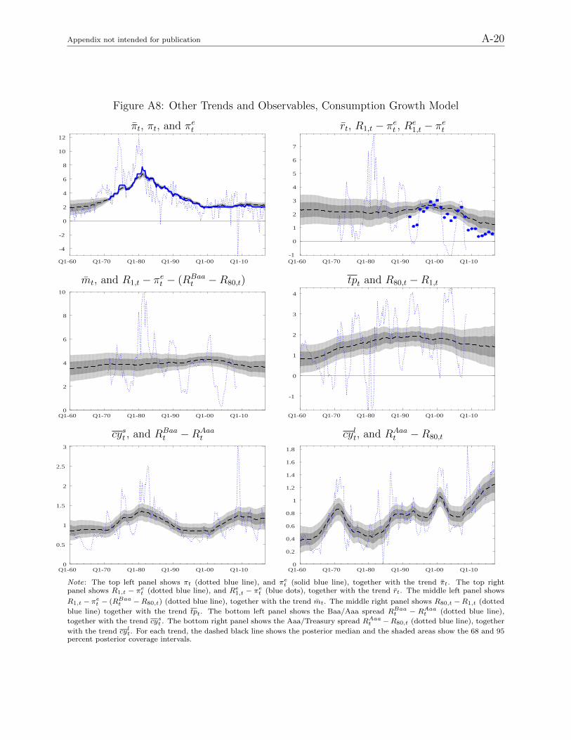
Appendix not intended for publication A-20

Figure A8: Other Trends and Observables, Consumption Growth Model

πt, πt, and πet rt, R1,t − πet , Re1,t − πet

Q1-60 Q1-70 Q1-80 Q1-90 Q1-00 Q1-10

-4

-2

0

2

4

6

8

10

12

Q1-60 Q1-70 Q1-80 Q1-90 Q1-00 Q1-10-1

0

1

2

3

4

5

6

7

mt, and R1,t − πet − (RBaat −R80,t) tpt and R80,t −R1,t

Q1-60 Q1-70 Q1-80 Q1-90 Q1-00 Q1-100

2

4

6

8

10

Q1-60 Q1-70 Q1-80 Q1-90 Q1-00 Q1-10

-1

0

1

2

3

4

cyst , and RBaat −RAaa

t cylt, and RAaat −R80,t

Q1-60 Q1-70 Q1-80 Q1-90 Q1-00 Q1-100

0.5

1

1.5

2

2.5

3

Q1-60 Q1-70 Q1-80 Q1-90 Q1-00 Q1-100

0.2

0.4

0.6

0.8

1

1.2

1.4

1.6

1.8

Note: The top left panel shows πt (dotted blue line), and πet (solid blue line), together with the trend πt. The top rightpanel shows R1,t − πet (dotted blue line), and Re1,t − πet (blue dots), together with the trend rt. The middle left panel shows

R1,t − πet − (RBaat −R80,t) (dotted blue line), together with the trend mt. The middle right panel shows R80,t −R1,t (dotted

blue line) together with the trend tpt. The bottom left panel shows the Baa/Aaa spread RBaat − RAaat (dotted blue line),

together with the trend cyst . The bottom right panel shows the Aaa/Treasury spread RAaat −R80,t (dotted blue line), together

with the trend cylt. For each trend, the dashed black line shows the posterior median and the shaded areas show the 68 and 95percent posterior coverage intervals.

Appendix not intended for publication A-21

Figure A9: yt, Λyt, and yt; Consumption Growth Model

πt πet R1,t

Q1-60 Q1-70 Q1-80 Q1-90 Q1-00 Q1-10-5

0

5

10

Pi

Q1-60 Q1-70 Q1-80 Q1-90 Q1-00 Q1-10

-5

0

5

Q1-60 Q1-70 Q1-80 Q1-90 Q1-00 Q1-100

2

4

6

EPi

Q1-60 Q1-70 Q1-80 Q1-90 Q1-00 Q1-10

-0.5

0

0.5

1

Q1-60 Q1-70 Q1-80 Q1-90 Q1-00 Q1-100

5

10

15BILL

Q1-60 Q1-70 Q1-80 Q1-90 Q1-00 Q1-10

-5

0

5

Re1,t R80,t RAaa

t

Q1-60 Q1-70 Q1-80 Q1-90 Q1-00 Q1-100

2

4

6

8

EBILL

Q1-60 Q1-70 Q1-80 Q1-90 Q1-00 Q1-10

-2

0

2

4

Q1-60 Q1-70 Q1-80 Q1-90 Q1-00 Q1-100

5

10

TBlong

Q1-60 Q1-70 Q1-80 Q1-90 Q1-00 Q1-10

-4

-2

0

2

4

Q1-60 Q1-70 Q1-80 Q1-90 Q1-00 Q1-100

5

10

15AAA

Q1-60 Q1-70 Q1-80 Q1-90 Q1-00 Q1-10-4

-2

0

2

4

RBaat ∆ct

Q1-60 Q1-70 Q1-80 Q1-90 Q1-00 Q1-100

5

10

15

BAA

Q1-60 Q1-70 Q1-80 Q1-90 Q1-00 Q1-10

-4

-2

0

2

4

6

Q1-60 Q1-70 Q1-80 Q1-90 Q1-00 Q1-10

-10

-5

0

5

dC

Q1-60 Q1-70 Q1-80 Q1-90 Q1-00 Q1-10

-10

-5

0

5

Note: For each variable the top panel shows the data yt and the trend component Λyt, and the bottom panel shows thestationary component yt. For each latent variable, the dashed black line shows the posterior median and the shaded areas showthe 68 and 95 percent posterior coverage intervals.

Appendix not intended for publication A-22

D Robustness – VAR (Section II)

Table A1: Change in Trends, 1998Q1-2016Q4 – Robustness

(1) (2) (3) (4)

Default Loose PriorInflation

Term SpreadProductivity

rt-1.46∗∗

[-1.80, -1.11]

(-2.12, -0.76)

-1.56∗∗

[-2.06, -0.98]

(-2.51, -0.34)

-1.27∗∗

[-1.61, -0.92]

(-1.92, -0.57)

-1.61∗∗

[-2.00, -1.19]

(-2.36, -0.75)

mt-0.08

[-0.40, 0.24]

(-0.70, 0.56)

-0.38

[-0.91, 0.24]

(-1.40, 0.91)

-0.32

[-0.64, -0.00]

(-0.95, 0.32)

-0.76

[-1.17, -0.35]

(-1.55, 0.08)

gt-0.72

[-1.10, -0.32]

(-1.47, 0.09)

βt-0.05

[-0.21, 0.12]

(-0.38, 0.29)

−cyt-1.38∗∗

[-1.58, -1.17]

(-1.78, -0.97)

-1.18∗∗

[-1.48, -0.88]

(-1.78, -0.56)

-0.95∗∗

[-1.16, -0.73]

(-1.37, -0.51)

-0.84∗∗

[-1.05, -0.63]

(-1.27, -0.41)

−cyst(safety)

-0.69∗∗

[-0.83, -0.54]

(-0.97, -0.40)

-0.46∗∗

[-0.65, -0.28]

(-0.85, -0.09)

-0.44∗∗

[-0.59, -0.29]

(-0.73, -0.15)

-0.39∗∗

[-0.54, -0.24]

(-0.68, -0.10)

−cylt(liquidity)

-0.69∗∗

[-0.82, -0.55]

(-0.95, -0.42)

-0.72∗∗

[-0.89, -0.54]

(-1.06, -0.36)

-0.51∗∗

[-0.64, -0.37]

(-0.76, -0.24)

-0.45∗∗

[-0.58, -0.32]

(-0.71, -0.19)

∆Prodt-1.06

[-1.57, -0.54]

(-2.05, 0.01)

Note: The table shows the change in the trends for the different specifications described in section II.D, the model with default(column (1)), loose prior (column (2)), inflation trends in the term spread (column (3)), and labor productivity (column (4)).For each trend, the table shows the posterior median, the 68 (square bracket) and 95 (round bracket) percent posterior coverageintervals. The ∗∗ symbol indicates that the decline is significant, in that the 95 percent coverage intervals do not include zero.

Appendix not intended for publication A-23

Figure A10: Posterior Distribution of γtp – Model with Inflation Affecting the Nominal

Term Premium

0 0.1 0.2 0.3 0.4 0.5 0.60

1

2

3

4

5

6

7

8

Note: The figure shows the posterior distribution of γtp. The prior is an expoential with mean .10.

Appendix not intended for publication A-24

Figure A11: Trends and Observables, Inflation Affecting the Nominal Term Premiuml

πt, πt, and πet rt, R1,t − πet , Re1,t − πet

Q1-60 Q1-70 Q1-80 Q1-90 Q1-00 Q1-10

-4

-2

0

2

4

6

8

10

12

Q1-60 Q1-70 Q1-80 Q1-90 Q1-00 Q1-10-1

0

1

2

3

4

5

6

7

mt, and R1,t − πet − (RBaat −R80,t) tpt and R80,t −R1,t

Q1-60 Q1-70 Q1-80 Q1-90 Q1-00 Q1-100

2

4

6

8

10

Q1-60 Q1-70 Q1-80 Q1-90 Q1-00 Q1-10

-1

0

1

2

3

4

cyst , and RBaat −RAaa

t cylt, and RAaat −R80,t

Q1-60 Q1-70 Q1-80 Q1-90 Q1-00 Q1-100

0.5

1

1.5

2

2.5

3

Q1-60 Q1-70 Q1-80 Q1-90 Q1-00 Q1-100

0.2

0.4

0.6

0.8

1

1.2

1.4

1.6

1.8

Note: The top left panel shows πt (dotted blue line), and πet (solid blue line), together with the trend πt. The top rightpanel shows R1,t − πet (dotted blue line), and Re1,t − πet (blue dots), together with the trend rt. The middle left panel shows

R1,t − πet − (RBaat −R80,t) (dotted blue line), together with the trend mt. The middle right panel shows R80,t −R1,t (dotted

blue line) together with the trend tpt. The bottom left panel shows the Baa/Aaa spread RBaat − RAaat (dotted blue line),

together with the trend cyst . The bottom right panel shows the Aaa/Treasury spread RAaat −R80,t (dotted blue line), together

with the trend cylt. For each trend, the dashed black line shows the posterior median and the shaded areas show the 68 and 95percent posterior coverage intervals.

Appendix not intended for publication A-25

E Additional Table – DSGE (Section III)

Table A2: DSGE Parameter Estimates

Prior Posterior

Parameter Type Mean SD Mean 90.0% Lower Band 90.0% Upper Band

Steady State

100γ N 0.400 0.100 0.381 0.313 0.450α N 0.300 0.050 0.177 0.151 0.201100(β−1 − 1) G 0.250 0.100 0.201 0.100 0.301σc N 1.500 0.370 1.097 0.922 1.282h B 0.700 0.100 0.503 0.436 0.574νl N 2.000 0.750 2.614 1.808 3.419δ - 0.025 0.000 0.025 0.025 0.025Φ - 1.000 0.000 1.000 1.000 1.000S′′ N 4.000 1.500 1.556 1.153 2.037ψ B 0.500 0.150 0.558 0.408 0.712L N -45.000 5.000 -47.415 -48.910 -45.793λw - 1.500 0.000 1.500 1.500 1.500π∗ - 0.500 0.000 0.500 0.500 0.500g∗ - 0.180 0.000 0.180 0.180 0.180

Nominal Rigiditiesζp B 0.500 0.100 0.945 0.931 0.960ζw B 0.500 0.100 0.906 0.867 0.948ιp B 0.500 0.150 0.237 0.098 0.365ιw B 0.500 0.150 0.583 0.360 0.801εp - 10.000 0.000 10.000 10.000 10.000εw - 10.000 0.000 10.000 10.000 10.000

Policyψ1 N 1.500 0.250 2.294 1.973 2.620ψ2 N 0.120 0.050 0.206 0.148 0.265ψ3 N 0.120 0.050 0.317 0.270 0.363ρR B 0.750 0.100 0.848 0.809 0.888ρrm B 0.500 0.200 0.229 0.139 0.318

Financial FrictionsF (ω) - 0.030 0.000 0.030 0.030 0.030γ∗ - 0.990 0.000 0.990 0.990 0.990ζsp,b B 0.050 0.005 0.047 0.039 0.055SP∗ G 1.000 0.100 1.039 0.878 1.189cyl∗ - 0.117 0.000 0.117 0.117 0.117cys∗ - 0.065 0.000 0.065 0.065 0.065

Exogenous Processesρg B 0.500 0.200 0.983 0.971 0.996ρµ B 0.500 0.200 0.975 0.955 0.995ρzp B 0.500 0.200 0.898 0.764 0.974ρz B 0.500 0.200 0.942 0.910 0.976ρcyp,l - 0.990 0.000 0.990 0.990 0.990

Appendix not intended for publication A-26

Table A2: DSGE Parameter Estimates

Prior Posterior

Parameter Type Mean SD Mean 90.0% Lower Band 90.0% Upper Band

ρcy,l B 0.500 0.200 0.639 0.357 0.931ρcyp,s - 0.990 0.000 0.990 0.990 0.990ρcy,s B 0.500 0.200 0.649 0.425 0.910ρσω B 0.750 0.150 0.628 0.488 0.873ρπ∗ - 0.990 0.000 0.990 0.990 0.990ρλf B 0.500 0.200 0.791 0.677 0.911ρλw B 0.500 0.200 0.497 0.190 0.858ηλf B 0.500 0.200 0.630 0.429 0.848ηλw B 0.500 0.200 0.499 0.217 0.816ηgz B 0.500 0.200 0.434 0.132 0.722σg IG 0.100 2.000 2.234 2.039 2.418σµ IG 0.100 2.000 0.477 0.305 0.640σzp IG 0.100 2.000 0.095 0.047 0.158σz IG 0.100 2.000 0.526 0.472 0.581σcyp,l IG 0.013 100.000 0.013 0.012 0.015σcy,l IG 0.100 2.000 0.092 0.040 0.150σcyp,s IG 0.013 100.000 0.011 0.010 0.013σcy,s IG 0.100 2.000 0.124 0.057 0.178σσω IG 0.050 4.000 0.556 0.178 0.776σπ∗ IG 0.030 6.000 0.054 0.044 0.064σλf IG 0.100 2.000 0.079 0.062 0.096σλw IG 0.100 2.000 0.379 0.333 0.429σrm IG 0.100 2.000 0.229 0.206 0.251σ1,r IG 0.200 4.000 0.096 0.075 0.117σ2,r IG 0.200 4.000 0.087 0.068 0.106σ3,r IG 0.200 4.000 0.089 0.069 0.109σ4,r IG 0.200 4.000 0.086 0.067 0.103σ5,r IG 0.200 4.000 0.088 0.068 0.108σ6,r IG 0.200 4.000 0.094 0.071 0.115σ7,r IG 0.200 4.000 0.236 0.111 0.375σ8,r IG 0.200 4.000 0.241 0.108 0.386σ9,r IG 0.200 4.000 0.242 0.111 0.374σ10,r IG 0.200 4.000 0.248 0.107 0.399σ11,r IG 0.200 4.000 0.247 0.107 0.400σ12,r IG 0.200 4.000 0.245 0.108 0.390

Measurementδgdpdef N 0.000 2.000 -0.003 -0.049 0.043γgdpdef N 1.000 2.000 1.036 0.965 1.108ρgdp N 0.000 0.200 0.077 -0.137 0.293ρgdi N 0.000 0.200 0.946 0.909 0.986%gdp N 0.000 0.400 -0.138 -0.774 0.466ρgdpdef B 0.500 0.200 0.499 0.367 0.636ρpce B 0.500 0.200 0.269 0.064 0.467ρAaa B 0.500 0.100 0.621 0.484 0.754ρBaa B 0.500 0.100 0.810 0.736 0.892

Appendix not intended for publication A-27

Table A2: DSGE Parameter Estimates

Prior Posterior

Parameter Type Mean SD Mean 90.0% Lower Band 90.0% Upper Band

ρ10y B 0.500 0.200 0.959 0.935 0.984ρtfp B 0.500 0.200 0.175 0.073 0.270σgdp IG 0.100 2.000 0.255 0.213 0.297σgdi IG 0.100 2.000 0.306 0.271 0.340σgdpdef IG 0.100 2.000 0.164 0.146 0.181σpce IG 0.100 2.000 0.101 0.083 0.119σAaa IG 0.100 2.000 0.024 0.021 0.028σBaa IG 0.100 2.000 0.049 0.042 0.055σ10y IG 0.750 2.000 0.124 0.113 0.135σtfp IG 0.100 2.000 0.749 0.678 0.820

Note: T N, B and G stand, respectively, for Normal, Beta and Gamma distributions. For Inverse Gamma (IG) distributions,we report the coefficients τ and ν instead of the prior mean and SD.

References

Aruoba, S. Boragan and Frank Schorfheide, “Insights from an Estimated Search-BasedMonetary Model with Nominal Rigidities,” Working Paper, 2008.

Bernanke, Ben, Mark Gertler, and Simon Gilchrist, “The Financial Accelerator in aQuantitative Business Cycle Framework,” in John B. Taylor and Michael Woodford, eds.,Handbook of Macroeconomics, Vol. 1C, North Holland, Amsterdam, 1999.

Boivin, Jean and Marc P. Giannoni, “DSGE Models in a Data Rich Enviroment,”NBER Working Paper, 2006, 12772.

Christiano, Lawrence J., Martin Eichenbaum, and Charles L. Evans, “NominalRigidities and the Dynamic Effects of a Shock to Monetary Policy,” Journal of PoliticalEconomy, 2005, 113, 1–45.

, Roberto Motto, and Massimo Rostagno, “The Great Depression and the Friedman-Schwartz Hypothesis,” Journal of Money, Credit and Banking, 2003, 35, 1119–1197.

, , and , “Risk Shocks,” American Economic Review, 2014, 104 (1), 27–65.

De Graeve, Ferre, “The External Finance Premium and the Macroeconomy: US Post-WWII Evidence,” Journal of Economic Dynamics and Control, 2008, 32 (11), 3415 –3440.

Del Negro, Marco and Stefano Eusepi, “Fitting Observed Inflation Expectations,”Journal of Economic Dynamics and Control, 2011, 35, 2105–2131.

Durbin, James and Siem Jan Koopman, “A Simple and Efficient Simulation Smootherfor State Space Time Series Analysis,” Biometrika, 2002, 89 (3), 603–616.

Appendix not intended for publication A-28

Greenwood, Jeremy, Zvi Hercowitz, and Per Krusell, “Long-Run Implications ofInvestment-Specific Technological Change,” American Economic Review, 1998, 87 (3),342–36.

Laseen, Stefan and Lars E.O. Svensson, “Anticipated Alternative Policy-Rate Paths inPolicy Simulations,” International Journal of Central Banking, 2011, 7 (3), 1–35.

Primiceri, Giorgio, “Why Inflation Rose and Fell: Policymakers’ Beliefs and US PostwarStabilization Policy,” Quarterly Journal of Economics, 2006, 121, 867–901.

Sargent, Thomas J., The Conquest of American Inflation, Princeton University Press,Princeton, 1999.

Sims, Christopher A., “Comment on Cogley and Sargent’s ‘Evolving post World WarII U.S. Inflation Dynamics’ ,” in Ben S. Bernanke and Kenneth Rogoff, eds., NBERMacroeconomics Annual 2001, Vol. 16, MIT Press, Cambridge, 2002, pp. 373–379.

Smets, Frank and Raf Wouters, “Shocks and Frictions in US Business Cycles: ABayesian DSGE Approach,” American Economic Review, 2007, 97 (3), 586 – 606.