* shi4@indiana.edu ° xu51@indiana.edu

Case Study Final Report

Inquiry on factors affecting units sold of products in specific Kroger Stores

Cheng Shi*, Xiaohan Xu°

Indiana University

April 24, 2015

Background: Dunnhumby is a UK-based Customer Service company. Its primary business is analyzing

data from nearly one billion customers worldwide with their willingness and demand in order to assist

corporations to make decisions and maximize their benefits. It is an independent company in the United

Kingdom but owned by Kroger Company in the United States. The Kroger Company is an American

retailer, which is the second-largest general retailer and has the largest revenue of supermarket chain.

Dunnhumby collected the data of customers from Kroger and use appropriate tools to analysis the data

with purpose of aiding Kroger Company better develop business.

1 Introduction

Our team was given an Excel file from Breakfast at the Frat, supported by Dunnhumby, containing sales

and promotional information from a sampling of 79 stores with 58 unique UPC (Universal Product Code)

over 156 week beginning from January 2009 to December 2011. The products were represented by UPC

and classified into 4 categories: BAG SNACKS, COLD CEREALS, FROZEN PIZZA, and ORAL

HYGIENE PRODUCTS. There are 24 variables, which are symbolic names containing some known or

unknown quantity or categorical values, including BASE_PRICE, DISPLAY, FEATURE, PRICE,

STORE_NUM, TPR_ONLY, UNITS, WEEK_END_DATE and UPC, etc. Each variable has a precise

description in the given database. For example, UNITS refers to units sold. PRICE refers to actual amount

charged for the products at shelf. UPC refers to specific identifiers of products. HHS refers to number of

purchasing households. DISPLAY refers to products that were parts of in-store promotional display.

TPR_ONLY refers to temporary price reduction only (i.e., shelf tag only, products were reduced in price

but not on display or in an advertisement). There were four sheets including Glossary, dh_Store Lookup,

dh_Products Lookup and dh_Transaction Data. In Glossary sheet, it listed names and descriptions of all

variables. In dh_ Store Lookup sheet, it included Store ID, name, address, parking space, store size and

average weekly baskets sold in each store. In dh_Products Lookup, it offered UPC, descriptions of

products, manufacturer, subcategory and product size. In dh_transaction data, there were 524,950 rows

and 13 columns. The sheet contains WEEK_END_DATE, STORE NUMBER, UPC, UNITS, VISITS,

HHS, SPEND, PRICE, BASE_PRICE, FEATURE, DISAPLY, and TPR_ONLY. In addition, we were

also given some examples of questions based on the data set. For example, what is the range of prices

offered on products? What will happen to unit sales if the price changes by X%? What is the impact on

sales of promotions, displays, or being featured in the circular? How do the above differ by store price tier

(e.g. upscale stores vs. value stores)? If you were the retailer, for which products would you be more

likely to increase the price to improve profits? Why? We were then motivated and inspired to begin to

look at our data, solve those example questions and come up with our own questions.

We have been given 500,000 data. The best thing is that the database is very fertile, and we can play

around the data and use the data to discover the relationship between units sold and price and also other

factors that affect units in order to give a good prediction to maximize total revenue. The bad thing is that

the dataset is so big that we cannot analyze the whole dataset at the same time. Hence, we decided to

zoom in and focus just one specific store with one specific product, and then zoom out to several stores

with several products.

2

0

20

40

60

80

100

14

-Ja

n-0

9

14

-Fe

b-0

9

14

-Ma

r-0

9

14

-Ap

r-0

9

14

-Ma

y-0

9

14

-Ju

n-0

9

14

-Ju

l-0

9

14

-Au

g-0

9

14

-Se

p-0

9

14

-Oct

-09

14

-No

v-0

9

14

-De

c-0

9

14

-Ja

n-1

0

14

-Fe

b-1

0

14

-Ma

r-1

0

14

-Ap

r-1

0

14

-Ma

y-1

0

14

-Ju

n-1

0

14

-Ju

l-1

0

14

-Au

g-1

0

14

-Se

p-1

0

14

-Oct

-10

14

-No

v-1

0

14

-De

c-1

0

14

-Ja

n-1

1

14

-Fe

b-1

1

14

-Ma

r-1

1

14

-Ap

r-1

1

14

-Ma

y-1

1

14

-Ju

n-1

1

14

-Ju

l-1

1

14

-Au

g-1

1

14

-Se

p-1

1

14

-Oct

-11

14

-No

v-1

1

14

-De

c-1

1

UNITS

2 Statement of Research Problem

By intuition, we were curious about discount, so we simply used base price minus price as discount.

Then, we used Excel to do some essential but vital analysis based on those data sheet. We got the basic

features of data by observing and calculating the maximum, minimum and range of different variables

like units, visits, prices and discount. In addition, we created some useful graphs like histogram,

frequency distribution, scattered plot and time series of those variables. We found that different stores

have different store size and 22 stores do not even have the data of parking space like store 11757 (KY)

Mainstream, store 15531 (OH) Value, Store 4503(TX) upscale and store 4245(IN) Mainstream. Based on

our experiences, Kroger Company not only owns large area of free parking space but also has its own gas

stations in the parking area. Therefore, for those stores without parking space, we considered that it might

due to missing data because Kroger is a supermarket, and parking space is vital element for a store to

attract its customers.

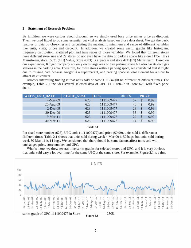
Another interesting finding is that units sold of same UPC might be different at different times. For

example, Table 2.1 includes several selected data of UPC 1111009477 in Store 623 with fixed price

$0.99.

WEEK_END_DATE STORE_NUM UPC UNITS PRICE

4-Mar-09 623 1111009477 57 $ 0.99

26-Aug-09 623 1111009477 46 $ 0.99

2-Dec-09 623 1111009477 28 $ 0.99

30-Dec-09 623 1111009477 36 $ 0.99

9-Mar-11 623 1111009477 29 $ 0.99

30-Mar-11 623 1111009477 14 $ 0.99

For fixed store number (623), UPC code (1111009477) and price ($0.99), units sold is different at

different times. Table 2.1 shows that units sold during week 4-Mar-09 is 57 bags, but units sold during

week 30-Mar-11 is 14 bags. We considered that there should be some factors affect units sold with

unchanged price, store number and UPC.

What’s more, we drew several time series graphs for selected stores and UPC, and it is very obvious

that units sold vary a lot over time for the same UPC at the same store. For example, Figure 2.1 is a time

series graph of UPC 1111009477 in Store 2505.

Table 2.1

Figure 2.1

3

In Figure 2.1, sales of items vary a lot over times based on time series. We observed that there are three

peaks: The first one is between 14-Dec-09 and 14-Jan-10; the second one is between 14-Dec-10 and 14-

Jan-11; and the third one is around 14-Dec-11. The sales significantly increased on Dec 14th for each

year. Conclusion: project is challenging.

Based on those findings, we want to find a focus and define our main purpose for our project. Since

the information we were given of sales of Kroger Company, the largest supermarket chain in USA by

revenue, we stated that the purpose of our team is to maximize total profit. However, we were not given

any costs for any of these stores, so we simplified the purpose to maximize total revenue. Since Kroger

set up their own price for every products, and we don’t know how they determine the price level, we will

consider that quantity is the dependent variable, and price is the independent variable. We wonder what

independent variables will have impact on our dependent variable, units sold. By intuition, our main focus

is the relationship between units sold and price, and we will also consider the relationship between units

sold and other factors such as display, holiday, feature, and discount by building up an appropriate model.

3 Discussion of Mathematical Fields Used in Working On the Problem

In this section, we will discuss our two fundamental mathematical tools to analysis our main focus, the

relationship between units sold and price and the relationship between units sold and holiday. We will

discuss linear regression model in section 3.1 and hypothesis testing in section 3.2. Both discussions will

be theoretical.

3.1 Linear Regression

In statistic, linear regression is an approach for modeling the relationship between a scalar dependent

variable y and one or more explanatory variables (or independent variable) denoted X. The case of one

explanatory variable is called simple linear regression. For more than one explanatory variable, the

process is called multiple linear regression. Simple linear regression functions by assuming that the

variables x and y have a linear relationship within the given set of data. (Stock, James H. Introduction to

Econometrics.) There are three main reasons why we want to use linear regression model to analysis the

relationship between units sold and other factors. The first reason is that linear relationship is the simplest

relationship between two variables. Therefore, we can first assume that units had the linear relationship

with other factors like price. For example, we assume that the linear equation for units and price,

units=slope * price + constant; linear equation for discount, units=slope*discount +constant. By nature

logic, as price increases, units sold should decreases. And as discount increases, the sales will increases.

Therefore, we expect that the slope would be negative for price and positive for discount. Secondly, after

simple regression, we can use multiple regression which allows us to figure out the relationships of units

with more than one explanatory variables. The last reason is for future prediction. According to the linear

regression based on data of three years, we can use the linear equation to predict the which factor has

more and effects on units and which factor may lose its power to explain the units sold as time goes by.

Those analysis are main evidence for us to set future prices and make racial decision and appropriate

adjustment.

We want to introduce an important theorem called “Gauss-Markov Theorem” to help explain our data

and solve our problems. In statistics, the Gauss–Markov theorem was named after Carl Friedrich Gauss

and Andrey Markov, and it assumes that the errors have expectation zero and are uncorrelated and each

error has equal variances in a linear regression model. By Gauss-Markov theorem, given the classical

assumption, the OLS (Ordinary Least Squares) estimators are BLUE (Best Linear Unbiased Estimator).

The theorem says that OLS estimators have minimum variance among linear and unbiased estimators and

hence Gauss-Markov does not say that they are the best of all possible estimators. The theorem does not

depend on any distributional assumptions like normality.

Classical Assumptions includes five parts:

A.1: In the population model, Y is related to X and error e as: Y=𝛽1 + 𝛽2*X+ e, which means the

population is linear.

4

A.2: (𝑥𝑖, 𝑦𝑖), i=1, 2, 3…,n, are random samples from the population model.

A.3: The sample outcome of X, {𝑥1,𝑥2, … … . 𝑥𝑛 } are not all the same values. There are some variation in

the values of xi.

A.4: E (𝑒𝑖|X)=0, for i=1,2…,n, which shows unbiasedness

A.5: Variance (𝑒𝑖)=𝜎2, i=1,2…,n, equal variance of all error 𝑒𝑖, which shows homoskedasticity.

(Stock, James H. 2011 Introduction to Econometrics. Chapter 4.5 The Sampling Distribution of the OLS

Estimators)

3.2 Hypothesis Testing

A statistical hypothesis testing is a method of statistical inference used for testing a statistical hypothesis.

Hypothesis testing contains two hypothesis: the null hypothesis and the alternative hypothesis. The null

hypothesis (Ho) corresponds to the idea that an observed difference is due to chance. The alternative

hypothesis (H1) is that the observed difference is real. In order to measure the difference between the real

case and what is expected on the null hypothesis, a test statistics is used (Freedman, Pisani and Purves.

Statistics. Page 477-481). Since the whole dataset is only a sample dataset, we will use t-test as the test

statistic (we are only able to calculate the sample standard deviation for the given data set). The test

statistics should give us a p-value after calculating by the computer (we can also do this by looking up the

table). We assume that the null hypothesis is right, p-value is not the chance of the null hypothesis being

right. What should we do after calculating the p-value? We should assign our significance level. The

significant level is the criterion used for rejecting the null hypothesis. Normally, the significant level is

denoted by α. The last step for hypothesis testing is how we should interpret it. We call it the decision

rule. Generally, the decision rule is interpreted as following: “If p-value < α, we reject Ho and conclude

that the difference is real; otherwise, we fail to reject Ho.”

For our hypothesis testing, we would like to test whether holiday increases units sold of products.

Furthermore, we would like to test holiday increases the average of units sold. The actual reason we

will introduce in section IV because the reason relates to our observation and thinking process. We set our

null hypothesis and alternative hypothesis:

Ho: µholiday ≤ µnonholiday

H1: µholiday > µnonholiday

µholiday denotes the average units sold on holiday, and µnonholiday denotes the average units sold not

on holiday.

We are required to calculate our t-score for our desired test statistic (t-test) for our hypothesis testing.

For our data set, units sold on holiday and units sold not on holiday have unequal sample sizes and

unequal sample variances, hence we will use the following formula to calculate the t-score.

𝑡 =𝑋1 − 𝑋2

S(𝑋1 − 𝑋2)

𝑋1 is the average of units sold on holiday. 𝑋2 is the average of units sold not on holiday. S(𝑋1 − 𝑋2) is the

standard deviation of (𝑋1 − 𝑋2) .

The formula of calculating S(𝑋1 − 𝑋2) is

S(𝑋1 − 𝑋2) = √𝑆1

2

𝑛1 +

𝑆22

𝑛2

𝑆1 is the standard deviation of units sold on holiday, 𝑆2 is the standard deviation of units sold not on

holiday. 𝑛1 is the sample size of units sold on holiday. 𝑛2 is the sample size of units sold not on holiday.

5

Here, we are assuming that 𝑋1 and 𝑋2 are independent. Otherwise, S(𝑋1 − 𝑋2) needs not be given by the

formulas. Example: 𝑋1 = 𝑋2. Then S(𝑋1 − 𝑋2) = 0.

Since we will use t-test, we should be aware of degree of freedom:

degree of freedom =(𝑆1

2

𝑛1 +𝑆2

2

𝑛2 )2

(𝑆1

2

𝑛1 )2

𝑛1 − 1+

(𝑆2

2

𝑛2 )2

𝑛2 − 1

(PASS Sample Size Software, chapter 425)

We had required mathematical tools and formulas to do our hypothesis test. The further question is

how we could calculate the p-value. At first, we wanted to use MATLAB because it is a useful

mathematical laboratory, and we are using it in our M466 class. However, one big issue of MATLAB is

that it takes dataset as matrices. We had already known that units sold on holiday and units sold not on

holiday have unequal sample sizes. We were not able to do some operations of linear algebra such as dot

product because some operations of linear algebra require units sold on holiday and units sold not on

holiday have equal sample size. Therefore, we decided to use R-studio. R-studio does not have

requirement of sample sizes, and we can see the running process of data on R-studio.

4 The Procedure of Using Required Mathematical Tools

In this section, we will discuss our steps of solving the problem by using linear regression and hypothesis

testing. We will summarize our observations and our analysis. We will introduce our thinking process

related to linear regression and several practical issues in section 4.1. In section 4.2, we will introduce our

procedure of using hypothesis testing. At the end of section 4.2, we will illustrate that our hypothesis

testing indicates some different results compared with linear regression model.

4.1 Linear Regression

Before regression, we defined and added some new variables we were interested to do research like

HOLIDAY_WEEK and DISCOUNT. For HOLIDAY_WEEK, we searched of popular traditional

holidays. music and sports days and finally added some these important days including Super

bowl(football), Oscar(movie), Grammy, NBA final(basketball), MLB final(baseball), VMA(MTV Video

Music Awards), AMA (American music awards), Christmas. Therefore, the definition for

HOLIDAY_WEEK is subjective. And for DISCOUNT, since we were only given BASE_PRICE and

PRICE, we defined BASE_PRICE minus PRICE as DISCOUNT for each product. To simplify our

process, we focus on one store for analysis, so we can just use the same process for other stores. Since

there were only 4 categories, we picked one UPC for each categories and then chose one store which

included 4 categories to run regression.

For example,

Store 367 UPC: 1111087395 FROZEN PIZZA;

Store 367 UPC: 1111038078 MOURTHWASHES;

Store 623 UPC: 1111009477 MINI TWIST PRETZELS;

Store 367 UPC: 1111085350 COLD CEREAL;

We used same method and regressions for the four products. For each UPC, we ran the simple

regressions and multiple regressions. At the beginning, we were not sure which predictors have effect

and how much variation of them can explain the variation of units sold. And we also want to get the most

fitted regression model. We tried using variables including PRICE, BASE_PRICE, DISCOUNT,

HOLIDAY_WEEK, FEATURE, DISPLAY, TPR_ONLY, VISITS and HHS in simple regression model.

However, according to the values of R-square, confidence interval and p-value, the BASE_PRICE and

TPR_ONLY are not helpful for our regression model because their corresponding R-square are 0%,

6

0.33% and p-value is 0.946, 0.478 from data store 367 UPC:1111087395 FROZEN PIZZA. And we did

more for other stores and products, the results are similar. The 0 R-Square indicates that the variation of

those regressions are not helpful to explain the variation of units sold. And the big p-value shows they are

not significant. In addition, HHS means the number of purchasing households and VISITS means the

number of unique purchases (baskets) that included the product. As the number of purchasing household

and their unique purchases that included the product increase, the units sold of the certain product will

definitely increase. HHS and VISITS are 99% correlated with units sold, so they are not the regressions

we are interested to do research. Then, we started to run simple regression (By STATA: Data Analysis

and Statistical Software) like below:

Example1

Store: 367 UPC: 1111038078 PL BL MINT ANTSPTC RINSE PRIVATE LABEL ORAL HYGIENE

PRODUCTS

MOUTHWASHES (ANTISEPTIC) 500 ML

. reg UNITS DISCOUNT

Source| SS df MS Number of obs = 138

-------------+------------------------------ F( 1, 136) = 4.01

Model| 27.3332081 1 27.3332081 Prob > F = 0.0473

Residual| 928.036357 136 6.82379674 R-squared = 0.0286

-------------+------------------------------ Adj R-squared = 0.0215

Total| 955.369565 137 6.97350048 Root MSE = 2.6122

UNITS| Coef. Std. Err. t P>|t| [95% Conf. Interval]

-------------+----------------------------------------------------------------

DISCOUNT| 1.062551 .530906 2.00 0.047 .0126524 2.11245

_cons| 3.833433 .2614647 14.66 0.000 3.316371 4.350496

------------------------------------------------------------------------------

The example I displayed is to explore the relationship between units sold and DISCOUNT for store

367 UPC: 1111038078, MOUTHWASHERES, which is one of categories, Oral hygiene products. There

are three main reasons for choosing this example. Firstly, for all MOUTHWASHES, only two regressors

PRICE and DISCOUNT are useful for our model to explain our sales. And a new problem occurred when

we ran this simple regression (Example1) and multiple regression (Example2). Secondly, it is nature to

think discount can help increase sales. However, based on the data from example1, the fact is not as what

people thought. The third reason is to compare the change of coefficient when we run regression with

PRICE and DISCOUNT separately and when we ran these two regressors together.

From the data, R-square is 2.86%, which means 2.86% of variation of units sold of mouthwashes

(500ml) in store 367, on average, can be explained by the variation of DISCOUNT. Therefore, based the

low R-square, we can conclude that DISCOUNT is not a good predictor for this certain product in this

store. The coefficient is about 1.06, which can be interpreted that as the discount of the product increases

by 1$, on average, the units sold will increase by 1.06. P-value is 0.047.

Another example we listed below is multiple regression for the same product in the same store. We

were faced with some new problems and interesting findings during running this regression. For example,

we ran a regression of MOUTHWASHERES using STATA, a note: “DISPLAY omitted because of

collinearity; HOLIDAY omitted because of collinearity” automatically appeared. Collinearity (or

multicollinear) is a phenomenon in which 2 or more predictor variables in a multiple regression model are

highly correlated.

Example2

Store:367 UPC:1111038078 PL BL MINT ANTSPTC RINSE PRIVATE LABEL ORAL HYGIENE

PRODUCTS

MOUTHWASHES (ANTISEPTIC) 500 ML

. reg UNITS PRICE DISPLAY FEATURE DISCOUNT HOLIDAY

7

note: DISPLAY omitted because of collinearity

note: HOLIDAY omitted because of collinearity

Source| SS df MS Number of obs = 21

-------------+------------------------------ F( 3, 17) = 0.90

Model| 13.5837657 3 4.5279219 Prob > F = 0.4622

Residual| 85.6543296 17 5.03848997 R-squared = 0.1369

-------------+------------------------------ Adj R-squared = -0.0154

Total| 99.2380952 20 4.96190476 Root MSE = 2.2447

------------------------------------------------------------------------------

UNITS| Coef. Std. Err. t P>|t| [95% Conf. Interval]

-------------+----------------------------------------------------------------

PRICE| -4.737992 3.027061 -1.57 0.136 -11.12453 1.648547

DISPLAY| 0 (omitted)

FEATURE| 1.269057 3.149502 0.40 0.692 -5.375811 7.913926

DISCOUNT| -1.900531 2.268131 -0.84 0.414 -6.685868 2.884806

HOLIDAY| 0 (omitted)

_cons| 11.13651 4.748398 2.35 0.031 1.118263 21.15475

------------------------------------------------------------------------------

For this multiple regression model, we used 5 predictors, PRICE, DISPLAY, FEATURE, DISCOUNT

and HOLIDAY_WEEK. However, the R-square is still low at 13.7%. And we observed that the p-values

are very large (over 0.1), which means PRICE, FEATURE and DISCOUNT were not significant in this

model. And then, we tried removing DISPLAY and HOLIDAY, and run regression of UNITS, PRICE,

FEATURE and DISCOUNT. The R-square is 12% and the DISCOUNT is still not significant with 0.382

p-value.

Some other interesting finding were received by comparing the results of run regression of PRICE and

DISPLAY together with separately. When we ran simple regression with units sold and PRICE, the

coefficient of PRICE was -2.206235 with R-square 9.26% and p-value 0. When we ran simple regression

with units sold and DISCOUNT, the coefficient of discount was +1.062551 with R-square 2.86% and p-

value 0. 047. However, if we ran multiple regression using both of PRICE and DISCOUNT as regressors,

the result changed a lot. (See Example3)

Examples3

Store:367 UPC:1111038078 PL BL MINT ANTSPTC RINSE PRIVATE LABEL ORALHYGIENE

PRODUCTS

MOUTHWASHES (ANTISEPTIC) 500 ML

reg UNITS PRICE DISCOUNT

Source| SS df MS Number of obs = 138

-------------+------------------------------ F( 2, 135) = 6.92

Model| 88.7867091 2 44.3933545 Prob > F = 0.0014

Residual| 866.582856 135 6.41913227 R-squared = 0.0929

-------------+------------------------------ Adj Rsquared = 0.0795

Total| 955.369565 137 6.97350048 Root MSE = 2.5336

------------------------------------------------------------------------------

UNITS| Coef. Std. Err. t P>|t| [95% Conf. Interval]

-------------+----------------------------------------------------------------

PRICE| -2.314459 .7480219 -3.09 0.002 -3.793816 -.8351017

DISCOUNT| -.1544378 .647959 -0.24 0.812 -1.43590 1.127026

_cons| 7.570749 1.234216 6.13 0.000 5.129849 10.01165

------------------------------------------------------------------------------

The coefficient of DISCOUNT becomes -.1544378(negative value), which means if the discount of the

product increases, the units sold will decreases, which sounds not reasonable. And compared with the R-

8

square 9.26% of simple regression using PRICE, the R-square 9.29% merely increases 0.03%, which

suggests the variation of DISCOUNT does not help to explain the variation of units sold. In addition, the

big p-value 0.812 of DISCOUNT shows that it is not significant. The reason for the result is that the two

regressors PRICE and DISCOUNT are highly correlated, which means that have similar movement with

each other.

In addition, we also did the regression for same UPC in different stores. We used the same explanatory

variables (PRICE, DISCOUNT, DISPLAY, FEATURE, and HOLIDAY_WEEK) to run regression. And

when we looked at units sold of FROZEN PIZZA UPC: 1111087395 in three different stores 367, 2505,

387, we found that, for same products in different stores, there were different data.

Example4

Store: 367/2505/387 UPC: 1111087395 FROZEN PIZZA

In store 367, R-square is 31.69% for PRICE, 44.57% for DISPLAY, 11.50% for FEATURE and p-values

are 0.

In store 2505, R-square is 43.20% for PRICE, 50.39% for DISPLAY, 39.56% for FEATURE and p-

values are 0.

In store 387, R-square is 42.20% for PRICE, 42.99% for DISPLAY, 25.66% for FEATURE and p-values

are 0.

We could get some results by comparing different data. For example, 31.39% shows that PRICE has

less effect on units sold of FROZEN PIZZA in store 367 than the other two stores. And 50.39% means

Display has more influence on sales of FROZEN PIZZA for store 2505 than the other two.

4.2 Hypothesis Testing

Before hypothesis testing, we first defined holiday. We defined Super Bowl, Grammy, Oscar, NBA Final,

VMA, MLB Final, AMA and Christmas to be holiday. All of these special dates except for Christmas are

Americans’ habits. Almost everyone watches the live of NBA, Super Bowl, etc. Christmas is a traditional

western holiday. Some other traditional holidays such as Easter, St. Patrick, we did not include them

because they are not as popular as Christmas.

After defining holidays, we randomly selected several products and stores because we could not do

hypothesis testing for all products in all stores, One major issue is that how we determine which stores

and which products that we will use for hypothesis testing. We cannot look at data and randomly choose

them because the way that we manually randomly choose data has bias. We decided to choose 10

products among four categories, so we gave each UPC code a number from 1 to n, where n is total

number of products among categories, and used excel command =RANDBETWEEN(1,n). This excel

command randomly gave us an integer between 1 to n, and then we chose the UPCs according to the

randomly selected number. After choosing the required UPCs, we would need to randomly select stores.

We gave each store a number from 1 to 79 and used the same randomly selected method with excel

command =RANDBETWEEN(1,79).

We randomly selected UPC codes, and then we randomly selected 10 stores according to the UPC

code that we chose. After observing the distribution of the selected data, it seems that units sold of

products on holiday is different from units sold of product not on holiday. Hence, we made a guess that

holiday affect units sold.

In order to simplify our hypothesis testing, we randomly reselected one product, frozen pizza with

UPC code 1111087395, and 10 stores that sell this product. We compared units sold on holiday and units

sold not on holiday of our selected product in different selected stores, and we found that units sold of

products on holiday is different from units sold of product not on holiday. Furthermore, we observed that

units sold of products on holiday is more than units sold of production not on holiday for most of stores,

but for some stores units sold of products on holiday is less than units sold of production not on holiday,

such as units sold in store 613, 623 and 2495, but the situation that units sold of products on holiday is

less than units sold of production not on holiday happens less frequently than the situation that units sold

of products on holiday is more than units sold of production not on holiday. However, these were our

9

conclusions based on our observations, and we were not certain that our conclusions were right by only

observing the data. Hence, we claim that holiday increases units sold and would like to use hypothesis

testing to prove our claims. Later on, we drew the frequency curve for units sold on holiday and units sold

not holiday. For example, Figure 4.2.1 and Figure 4.2.2 are frequency curves of units sold on holiday and

units sold not holiday for store 387 and Store 2277. The blue line represents units sold on holiday, and the

orange line represents units sold not on holiday.

The average units sold on holiday is higher than average units sold not holiday in

most of time, but not all the time. We observed that the average (mean = 15.30) of units sold on holiday is

more than the average (mean = 10.41) units sold not on holiday for store 387. However, the average

(mean = 10.70) of units sold on holiday is less than the average (mean = 15.30) units sold not on holiday

for store 2277. There are 8 stores that the average units sold on holiday is higher than average units sold

not holiday in our randomly selected 10 stores. We claim that the average units sold on holiday is higher

than average units sold not holiday frequently. Hence, we changed our test to testing holiday increases the

average of units.

Next, we were able to set our null hypothesis and alternative hypothesis:

Ho: µholiday ≤ µnonholiday

H1: µholiday > µnonholiday

µholiday denotes the average units sold on holiday, and µnonholiday denotes the average units sold not

on holiday.

We then calculated test statistics used R-studio to calculate the p-value. Since our focus is µholiday >

µnonholiday, our hypothesis testing is a 2 sample t-test with different sample size and right-tail test.

Therefore, the formula for p-value should be:

p-value = 1 - probability corresponding to our t-score.

Table 4.2.1 shows t-scores and p-values for 4 stores.

Store Number t-score p-value

387 0.89 19.02%

623 -0.64 73.66%

2277 -1.16 87.34%

2496 4.59 0.003%

The last step is to state our decision rule. For example: suppose we chose α=5%.

Normally, statisticians choose 5% to be the significance value, but it varies depending on situations.

a. For store 387, p-value=19.02% > α=5%, we fail to reject Ho.

Figure 4.2.1 Figure 4.2.2

Table 4.2.1

10

b. For store 623, p-value=73.66% > α=5%, we fail to reject Ho.

c. For store 2277, p-value=87.34% >α=5%, we fail to reject Ho.

d. For store 2495, p-value=0.003%< α=5%, we reject Ho and conclude that µholiday > µnonholiday..

After doing hypothesis testing, we summarized that holiday does not increase average units sold

significantly. The significant level we chose is α=5%. We showed four stores above, and only one store

has significant evidence to prove µholiday > µnonholiday, which implies that holiday increases average

units sold. Hence, we concluded that we do not have significant evidence that holiday increases average

units sold in this products. There exists some relationship between holiday and units sold, but units sold

also depends on the store, the UPC code, etc. Most of these hypothesis testing suggest that holiday has a

weak influence on sales.

5 The Solution of linear regression and hypothesis testing

For some of regression model, not all expected value of error for each x is 0, which violated the classical

assumption of OLS estimators. In classical assumption (A.4), E(ei|Xi)=0 shows unbiasedness. Therefore,

some estimators of parameters in our regression models are biased and the regression model is not fitted,

hence those models are not meaningful for us to do further research. For example, for both simple and

multiple regressions, collinearlity problems occur for HOLIDAY_WEEK and FEATURE of

MOUTHWAHSERS for store 367. The same problem with the multiple regression model using

DISOCUTN and PRICE of MOUTHWAHSERS for store 367. During the creation of regression models,

collinearity can occur. Although the overall model still can have good predictability, the collinearity will

cause invalid results for individual predictors. However, we still need to include them to run multiple

regression as our solution because highly correlated variables does not mean they are perfectly correlated

and when we add DISCOUNT to run regression, the coefficient of DISCOUNT changed a lot. If we just

ignore the effect of DISCOUNT and remove it from multiple regression model, we will overestimate the

effect of PRICE.

From the linear regression model, we observed that the dummy variable HOLIDAY_WEEK does not

fit a regression line. The correlation of units sold and HOLIAY_WEEK is very low which implies that the

linear relationship between units sold and HOLDAY_WEEK is very weak.

For hypothesis testing, we chose α=5% and we rejected 1 of 10 store and conclude that we do not have

significant evidence µholiday > µnonholiday. We recall that null hypothesis testing indicates that the

difference between two means are due to chance, introduced in section 3.2. For our case, we may

conclude that holiday affects units sold is due to chance, specifically holiday increases units sold is due to

chance. The reason that we may conclude but not confidently conclude is that we only did hypothesis

testing for on UPC in 10 stores, so we cannot draw a conclusion among all UPCs and all stores. There

exists some relationship between holiday and units sold that holiday affect units sold. Nevertheless, this

relationship is weak.

In summary, we conclude that linear relationship cannot describe the relationship between units sold

and holiday, and our linear regression model does not fit to predict how holiday affect units sold.

However, this does not mean that there does not exist relationship between units sold and holiday. In

summary, we concluded that there exists relationship between units sold and holiday, but it is not linear

relationship.

6 The implications of the research

In conclusion, although the linear regression suggests the holiday week does not have influence on units

sold of a product, but that does not mean there is no relationship between them. Based on the data of

hypothesis testing, the increase of units sold affected by HOLIDAY_WEEK is not significant. Therefore,

11

we might conclude that the factor of HOLIDAY_WEEK may affect the units sold for some categories of

product like small snacks but the effect is weak.

The first limitation is that we are unable to run all simple and multivariable regression for all different

products in different store. Therefore, what we can do is that we picked three stores and three products

based on category, which allows us to compare one product in different stores and different product in the

same store.

The second limitation is inaccurate definition for new added variables, HOLIDAY_WEEK and

DISCOUNT. And the problem occurs that there are several discounts are negative numbers, which sounds

unreasonable, but we still used them when run our regression.

The third limitation is that we cannot guarantee that our hypothesis testing is optimal. We only did

hypothesis testing for one UPC and 10 stores. Are we certain that our selected stores have reasonable

data? We did not consider outliers in our randomly selected sample. Hence, outliers may affect our

hypothesis testing.

The last limitation is our limited mathematical knowledge. None of us knows how to use other

mathematical or statistical methods to deal with the unknown relationship between holiday week and

units sold.

Acknowledge: Thanks Indiana Statistical Consulting Center for technology supports. Thanks Professor

Kevin Pilgrim for being our mentor. Thanks Professor Natasha Blitvic and Professor Bibo Jiang for being

our consultants.

12

Citation

Dunnhumby Official Website. http://www.dunnhumby.com/us/what-we-do

"Select Your Location." What We Do. N.p., n.d. Web. 23 Apr. 2015

Freeman, David A. "Statistical Models: Theory and Practice" 2 Edition ed.

N.p.: Cambridge UP;, April 27, 2009. Print.

Freedman, David, Robert Pisani, and Roger Purves. “Statistics”.

New York: Norton, 1978. Print.

"Sample Size & Power." NCSS. N.p., n.d. Web. 23 Apr. 2015.

Stock, James H. “Introduction to Econometrics.”

Upper Saddle River, NJ: Pearson Education, 2011. Print.

Wooldridge, Jeffrey M. “Introductory Econometrics: A Modern Approach.”

Mason, OH: South Western, Cengage Learning, 2009. Print.

Anawis, Mark A. "Dealing with Collinearity."

Scientific Computing. N.p., 15 Mar. 2013. Web. 23 Apr. 2015.

"Stata: Data Analysis and Statistical Software." Data Analysis and Statistical Software.

Web. 16 Apr. 2015.