Russian Gas Imports in Europe: How Does Gazprom...
32
79 The Energy Journal, Vol. 31, No. 4, Copyright 2010 by the IAEE. All rights reserved. * Corresponding author. Center for Economic Studies (Department of Economics) and KULeuven Energy Institute, Catholic University of Leuven (KULeuven), Naamsestraat 69, BE-3000 Leuven, Belgium. Currently at: European Commission, JRC, Institute for Energy, P.O. Box 2, 1755-ZG Petten, The Netherlands. E-mail: [email protected]. The views expressed are purely those of the author and may not in any circumstances be regarded as stating an official position of the European Commission. ** Center for Economic Studies (Department of Economics) and KULeuven Energy Institute, Catholic University of Leuven (KULeuven), Naamsestraat 69, BE-3000 Leuven, Belgium. E-mail: [email protected]. Russian Gas Imports in Europe: How Does Gazprom Reliability Change the Game? Joris Morbee* and Stef Proost** Europe’s dependence on Russian gas imports has been the subject of increasing political concern after gas conflicts between Russia and Ukraine in 2006 and 2009. This paper assesses the potential impact of Russian unreliability on the European gas market, and how it affects European gas import strategy. We also study to what extent Europe should invest in strategic gas storage capacity to mitigate the effects of possible Russian unreliability. The European gas import market is described by differentiated competition between Russia and a – more reliable – competitive fringe of other exporters. The results show that Russian contract volumes and prices decline significantly as a function of unreliability, so that not only Europe but also Russia suffers if Russia’s unreliability increases. For Europe, buying gas from more reliable suppliers at a price premium turns out to be generally more attractive than building strategic gas storage capacity. 1. INTRODUCTION In recent years, security of gas supply has been high on the political agenda in Europe. Gas import dependence of the European OECD bloc will increase from 45% in 2006 to 69% in 2030, according to the IEA (2008) Refer- ence Scenario. Russia plays a crucial role, given that it already supplies more than half of Europe’s gas imports and that it has the largest proven natural gas
Transcript of Russian Gas Imports in Europe: How Does Gazprom...

79
The Energy Journal, Vol. 31, No. 4, Copyright �2010 by the IAEE. All rights reserved.
* Corresponding author. Center for Economic Studies (Department of Economics) and KULeuvenEnergy Institute, Catholic University of Leuven (KULeuven), Naamsestraat 69, BE-3000Leuven, Belgium. Currently at: European Commission, JRC, Institute for Energy, P.O. Box 2,1755-ZG Petten, The Netherlands. E-mail: [email protected]. The views expressed arepurely those of the author and may not in any circumstances be regarded as stating an officialposition of the European Commission.
** Center for Economic Studies (Department of Economics) and KULeuven Energy Institute,Catholic University of Leuven (KULeuven), Naamsestraat 69, BE-3000 Leuven, Belgium.E-mail: [email protected].
Russian Gas Imports in Europe:How Does Gazprom Reliability Change the Game?
Joris Morbee* and Stef Proost**
Europe’s dependence on Russian gas imports has been the subject ofincreasing political concern after gas conflicts between Russia and Ukraine in2006 and 2009. This paper assesses the potential impact of Russian unreliabilityon the European gas market, and how it affects European gas import strategy.We also study to what extent Europe should invest in strategic gas storage capacityto mitigate the effects of possible Russian unreliability. The European gas importmarket is described by differentiated competition between Russia and a – morereliable – competitive fringe of other exporters. The results show that Russiancontract volumes and prices decline significantly as a function of unreliability, sothat not only Europe but also Russia suffers if Russia’s unreliability increases.For Europe, buying gas from more reliable suppliers at a price premium turnsout to be generally more attractive than building strategic gas storage capacity.
1. INTRODUCTION
In recent years, security of gas supply has been high on the politicalagenda in Europe. Gas import dependence of the European OECD bloc willincrease from 45% in 2006 to 69% in 2030, according to the IEA (2008) Refer-ence Scenario. Russia plays a crucial role, given that it already supplies morethan half of Europe’s gas imports and that it has the largest proven natural gas
IAEE
Sticky Note
Article from 2010, Volume 31, Number 4

80 / The Energy Journal
1. In this paper, the terms Europe and European refer to the EU-27 plus Norway, Switzerland andIceland, unless indicated otherwise.
2. It should be noted that the relation between Russia and Europe is very different from the relationbetween Russia and its neighboring states, which, before the price increase, were receiving gas fromRussia at prices below netback parity. In addition, it is suspected that Russia’s price increases inneighboring states are a prelude to deregulation of Russia’s domestic gas market, which currentlyalso has below-market prices. Both considerations imply Russia had understandable reasons for rais-ing prices to its neighbors. On the other hand, Russian gas prices for Europe in 2006 were alreadyin line with the prices in the middle column of Table 1, which made Europe a profitable and importantcustomer for Russia. Given that, in addition, Gazprom was trying to enter the downstream Europeangas market, Russia was unlikely to act in the same way towards Europe as it did towards Ukraine.Nevertheless, as a result of the Ukrainian gas crises, European politicians and gas consumers clearlystarted questioning the reliability of Russia as a gas supplier.
reserves in the world (BP, 2008).1 This has been a source of increasing politicalconcern, especially since 2006, when Russian gas export monopolist Gazpromlaunched an effort to increase the gas prices paid by Russia’s neighboring states,as shown in Table 1.
The price conflict in Ukraine sparked strong political reactions in Eu-rope, because it led to interruptions of gas supplies to Europe in the beginning of2006 and 2009. Energy supply security and in particular the potential unreliabilityof Russian gas imports became an important topic at EU summits and G8 meet-ings, and in bilateral discussions with Russia. After the second conflict in January2009, Czech Prime Minister Topolanek – then President of the European Council– even stated explicitly that “the EU must weaken its dependence on Russian gasimports” (IHT, Jan 28, 2009).2
Table 1. Gas Prices for Russia’s Neighboring States, in USD per tcm
Price on Increased price Price onCountry Dec 31, 2005 demanded by Gazprom Jan 1, 2007
Ukraine 50 230 130Belarus 46 200 100Georgia 100 235 235Moldova 80 (unknown) 170
Note: tcm � thousand cubic meters. Source: Press sources (2006).
This paper provides an economic perspective on Russia’s strategicposition in the European gas market by answering the following two researchquestions:
1. What is the potential impact of Russian unreliability on theEuropean gas market, and how does this affect European gas importdecisions?
2. To what extent should Europe invest in strategic gas storage capacityto mitigate the effects of potential Russian unreliability?

Russian Gas Imports in Europe / 81
We study long-term gas contracting in a non-cooperative setting, usinga partial equilibrium model of the European gas market, with differentiatedcompetition between one potentially unreliable ‘dominant firm’ (Russia) and areliable ‘competitive fringe’ of other non-European import suppliers. Russia’spotential unreliability is modeled by assuming that there is a probability thatdRussia does not comply with the long-term contracts it has signed: with proba-bility , Russia ‘defaults’ and withholds supply to increase its price to monopo-dlistic levels for a duration of four months.
The numerical analysis in this paper shows that it is not optimal forRussia to cut gas supplies to Europe completely during a crisis: rather, one canexpect Russia to reduce its gas supplies by roughly 40% during the four months,thereby temporarily increasing gas prices by roughly 40%. More importantly, theanalysis shows that not only Europe but also Russia suffers when Russia’s prob-ability of default increases. Indeed, as Russia becomes – or is perceived asdbecoming – more unreliable, Europe procures a larger volume of long-term gasimport contracts from the competitive fringe. In doing so, Europe makes itselfless dependent on Russia and therefore less vulnerable in the event of Russianwithholding. With increasing Russian unreliability, the volume of long-term gasimport contracts with Russia decreases while Russia has to grant an ever higherdiscount in its contracts. The resulting negative impact on Russia’s profits is notsufficiently counterbalanced by the gains it makes in case it does not comply withits contracts. As a result, Russia’s expected profits are found to decrease asRussia’s unreliability increases. As mentioned before, investments in strategic gasstorage capacity can reduce Europe’s vulnerability. However, the numerical sim-ulations show that strategic storage capacity is only attractive for Europe if Rus-sian unreliability is high ( of more than 30%) and storage capacity costs aredreduced by a factor 3 to 4 compared to typical current cost levels.
Earlier papers have studied Russian gas imports into Europe from dif-ferent perspectives. Hirschhausen et al. (2005) focus on the strategic interactionbetween Russia and transit countries such as Ukraine and Belarus. Grais andZheng (1996) analyze the quantity, price and transit fee of gas contracts betweenRussia and Europe, in a hierarchical three-stage Stackelberg game in which Russiais the leader, followed by the transit country, which in turn is followed by theresponse of European demand (factoring in a potential alternative gas supplier).They study the impact of exogenous shocks, e.g. an exogenous change in thepreference for Russian gas over other gas, and they mention reliability as a po-tential cause of such a shock. Our model has a non-cooperative multi-stage struc-ture similar to Grais and Zheng (1996), but goes a step further by explicitlyexamining how reliability affects the demand for Russian gas compared to gasfrom other suppliers: a demand shift resulting from a change in (un-)reliability isan endogenous effect in our model. In addition, our paper investigates investmentin strategic gas storage capacity. On the flip side, to keep the paper focused, wedo not model the strategic behavior of transit countries.
The effect of a Russian supply interruption has recently been examinedby Hartley and Medlock (2009): as part of their analysis of potential futures for

82 / The Energy Journal
3. Nordhaus (1974) also investigates import taxes, but it turns out that storage is the most specificresponse to supply security concerns. In this paper, storage shall therefore be used as the exemplifi-cation of a broader range of policy measures (e.g. import taxes, rationing, subsidies for renewableenergy, etc.).
4. Note in particular that an analysis of long-term contracts is not considered inconsistent with non-cooperative modeling. On the contrary, Boots et al. (2004) also use (non-cooperative) Cournot-Nashmodeling, which they justify by writing “competition can be expected to take place through quantities,since long-term take-or-pay contracts still prevail in the natural gas market” (Boots et al., 2004, p.74).
5. However, unlike this paper, the models of Boots et al. (2004) and Golombek et al. (1995, 1998)analyze a segmentation of the European market, based on country and/or type of consumer and/orseason. Our paper has only one aggregate demand curve. Note that Holz et al. (2008), as an exception,use non-linear demand curves.
Russian gas exports, they use a comprehensive numerical dynamic spatial equi-librium model to study the global supply chain repercussions of a scenario inwhich Russia withholds roughly one third of its gas supplies to Europe during afour-month period. Hartley and Medlock (2009) model the interruption as a de-terministic shock with exogenous size. In contrast, in our model, the size of theshock is endogenous, and more importantly, there is uncertainty as to whether theshock will occur. Our model provides an analytical study of how the anticipationof a possible shock – in other words, the perception of unreliability – altersstrategic decisions. Our methodology for modeling unreliability is taken from thepioneering paper by Nordhaus (1974), who analyzes oil supply interruptions usinga model with two regimes: a normal regime and a supply interruption regime,each with its probability. Like Nordhaus (1974), we investigate the option ofinvesting in storage capacity.3 However, in addition, our model analyzes the con-trast between an unreliable supplier and a reliable competitive fringe. In thissetting, gas import contracts with the reliable competitive fringe and investmentsin storage capacity are (imperfect) substitutes.
Since our paper studies long-term gas import contracts, there are simi-larities with the literature that deals with these contracts (such as Boucher et al.,1987, and Neuhoff and Hirschhausen, 2005) and with the ‘hold-up’ literature,such as Hubert and Ikonnikova (2004). However, an important difference betweenthe approach in this paper and the approach of Hubert and Ikonnikova (2004) orIkonnikova and Zwart (2009) is that the latter two papers use cooperative gametheory and explicitly model the negotiation/bargaining between the various par-ties. Our paper, in contrast, describes the gas market in a non-cooperative settingwith quantity competition, following the seminal work of Mathiesen et al. (1987),several well-known analyses such as Golombek et al. (1995, 1998), Boots et al.(2004) and more recent work such as Holz et al. (2008) and Lise et al. (2008).4
Most of this literature considers European consumers as price-takers with lineardemand, which is also the approach taken in this paper.5
On a broader microeconomic level, the analysis of this paper fits intothe literature on differentiated competition. Indeed, as will be shown in Section3, the contrast of a potentially unreliable gas import supplier (in this case: Russia)

Russian Gas Imports in Europe / 83
6. A case of elastic domestic supply is discussed in Annex E.7. For the sake of simplicity, our model does not go to the level of individual end-consumers such
as households, industrial users and power generators. Therefore, the term , as we will compute itCSbased on demand curve (1), is in fact the importer surplus. In practice, this surplus is somehowdivided into importers’ profits on the one hand and end-consumer surplus on the other hand. We willnot make that distinction, since it depends on market power and regulation in individual countries.We will simply refer to as ‘consumer surplus.’CS
and a set of reliable import suppliers (in this case: the competitive fringe of othernon-European import suppliers), results in a market structure similar to differ-entiated competition. Singh and Vives (1984) for example, compare Cournot andBertrand competition in differentiated duopoly, while Gaudet and Moreaux (1990)do the same for the particular case of nonrenewable natural resources. The maincontribution of our paper is that it introduces the notion of unreliability directlyinto the market structure of the European gas market.
2. MODEL OF THE EUROPEAN GAS MARKET
2.1. European Demand, Domestic Supply, and Objective Function
Europe is modeled as a large number of uncoordinated gas consumersand domestic gas producers, with an overarching government that can decide toinvest public funds in gas storage capacity. We assume Europe is a price-takerwith a linear long-run inverse demand curve for gas:
p(q)���bq (1)
European domestic producers supply an exogenous and fixed6 quantity , andqD
the remaining excess demand needs to be satisfied by non-European im-q�qD
ports. Short-run demand is also linear, but with a steeper slope :bSR
p (q)�p*�b •(q�q*) (2)SR SR
with p*, q* representing the long-run equilibrium.We assume that decisions on long-term gas import contracts and publicly
financed strategic storage capacity investments are based on a combination of theinterests of importers, end-consumers, domestic producers and taxpayers. Wetherefore assume that Europe maximizes the expected total ‘European surplus’
:E[S]
max E[S] with S�CS�P �G (3)D
where is the consumer surplus,7 represents the profits of domestic pro-CS PD
ducers, and is the public expenditure on gas storage capacity investments.Grepresents the interests of the recipients of marginal expenditures out of�G
general government revenue. Note that equation (3) assumes risk-neutrality.Annex D deals with the case of European risk aversion.

84 / The Energy Journal
8. This fairly standard model of industrial organization is described in multiple textbooks, e.g.Carlton and Perloff (2000, Chapter 4).
9. Hence, is exogenous, and there is perfect and complete information about it. The rationaled
for exogeneity of is that Russia’s decision-makers are also aware of the potential unreliability ofd
the Russian state, and that they do not have full control over Russia’s image of unreliability, nor overRussia’s actual behavior over the entire period for which gas contracts are signed. For instance,although Russia never cut gas supplies to Europe during the Ukrainian gas conflicts, the conflictnevertheless led to an increased perception of unreliability in Europe. As we will see later, our modelshows that if Russia had full control over its unreliability, it would be optimal for Russia to be perfectlyreliable ( ). Since we want to study the effects of increased unreliability (whether it is pursuedd�0deliberately or not), we make exogenous. In Section 5, we mention a different approach whichd
could lead to an endogenous .d
2.2. Non-European Gas Import Suppliers
Excess demand needs to be satisfied by signing long-term import con-tracts with non-European import suppliers. We assume that the non-Europeanimport suppliers have a dominant firm – competitive fringe structure.8 Russia isthe ‘dominant firm’ and the other non-European gas import suppliers are groupedtogether as the ‘competitive fringe.’
Russia is modeled as a monolithic entity, i.e. the Russian state is notdistinguished from the gas exporter Gazprom. Russia is assumed to be a risk-neutral profit maximizer. Russia is modeled to be unreliable: once the long-termcontracts have been signed, there is a probability that Russia temporarily doesdnot comply with its supply commitments, i.e. Russia ‘defaults.’ Conversely, thereis a probability that Russia complies with its long-term contracts during(1�d)the entire period. All participants know the parameter upfront.9 Russia’s long-drun marginal costs of production are assumed constant at .cR
The competitive fringe is a diversified set of current or potential futurenon-European gas import suppliers, including both pipeline and LNG supplies.Therefore, we assume that – as a group – the competitive fringe is reliable: evenif Russia defaults, the competitive fringe delivers the originally promised contractquantity at the originally promised contract price . This requires two as-q p0 0
sumptions. First, we assume that the long-term gas import contracts betweenEurope and the competitive fringe are not indexed on any gas spot market price,which would rise sharply in the event of Russian default. In practice, this con-dition is fulfilled since most current long-term gas import contracts contain littleor no indexation on gas spot market prices. Second, we assume that the compet-itive fringe players do not deviate from their contracts. This is a major assumption,which can be justified by the difference in scale between Russia and each of theother non-European import suppliers. Each of the other non-European importsuppliers has much less incentive to be unreliable because the market impact ofeach of them is much smaller. In addition, a supplier who is perceived as unre-liable could face the threat of being replaced by another supplier in the long term.Russia, on the other hand, is hard to replace completely in the long term, even ifit behaves unreliably.

Russian Gas Imports in Europe / 85
10. One could imagine offering interruptible contracts to industrial consumers at a discount. Wewill not consider that option in this paper.
11. Note that, while certain parts of the transportation cost can be estimated reasonably well (e.g.LNG shipping from overseas suppliers to Europe), transportation sometimes relies on transit countries(e.g. Ukraine), which leads to additional complexity. For example, Hirschhausen et al. (2005) explic-itly study the strategic considerations involved in gas transport from Russia to Europe via transit coun-tries Ukraine and Belarus. While these considerations are important, our paper focuses on the strategicinteraction between Europe and its import suppliers. We use OME (2002) estimates of the transit fees.
As we will see below in Section 2.3, the reliability of the competitivefringe does not mean that – in the event of Russian default – there would beprice discrimination between end-consumers of Russian gas and end-consumersof gas from the competitive fringe. There will be only one single end-consumerprice.10 However, the rents that result from the compliance of the competitivefringe in the event of Russian default accrue to European importers. Therefore,the most important implication of our assumption is that these rents are part ofthe European surplus function in equation (3), and are not part of the profits ofSthe competitive fringe. As for costs, we assume that the long-run marginal costcurve of the competitive fringe is linearly increasing: (with thec �d q q0 0 0 0
volume of long-term gas import contracts supplied by the competitive fringe, and, positive constants).c d0 0
The above-mentioned long-run marginal cost functions (i.e. for Rus-cR
sia, and for the competitive fringe) include not only production costs,c �d q0 0 0
but also transportation costs. The calibration for the numerical simulations ofSection 4 will take this into account.11 Finally, since this paper analyzes the gasmarket on an aggregated European level and does not model gas delivery to end-consumers, distribution costs are irrelevant.
2.3. Structure of the Game
The interaction between Europe, Russia and the competitive fringe, ismodeled as a game in three stages. Figure 1 explains the different stages of thegame. In a nutshell: in Stage 1, Europe decides how much to invest in strategicgas storage capacity; Stage 2 is the stage in which Europe signs long-term gasimport contracts with Russia and the competitive fringe; Stage 3 consists in theexecution of the long-term gas import contracts, in which Russia may or may notcomply with the long-term contracts it has signed. We represent the imported gasquantities by (Russia complies with long-term contracts), (Russia de-q qR,1 R,2
faults) and (competitive fringe). The corresponding prices are denoted ,q p0 R,1
and .p pR,2 0
Before describing each of the stages in detail, it is important to note thatthe stochastic outcome of Stage 3 influences the strategic interaction in Stage 2,because Europe and Russia factor the expected value of Stage-3 pay-offs intotheir decisions in Stage 2. In Stage 3, European surplus is either orS�S S�1
depending on whether Russia complies with its long-term contracts or not. InS2

86 / The Energy Journal
Figure 1. Timeline and Decisions in the Model Proposed in this Paper
Case 1 – Russia complies with long-term contracts:• Russia delivers
qR,1 as promised• Competitive
fringe delivers q0
Stage 1: Storage capacity investment decision
Stage 3:Execution of contracts
Europe decides construction of strategic gas storage capacity qS
Probability(1 – δ )
Probabilityδ
‘Nature’ decides whether Russia defaults or not (i.e., this is a probabilistic event)
Case 2 – Russia ‘defaults’:
• Russia delivers qR,2 (< qR,1)
• Competitive fringe delivers q0
‘Dominant firm – competitive fringe’ game, with Europe as price-taker:– Russia (dominant firm) decides to promise gas contract quantity qR,1
– Competitive fringe decides to promise gas contract quantity q0
– Europe’s inverse demand curves determine gas contract prices pR,1
Rp0 in response to q ,1 and q0
123
Timeline Decisions (decision-makers in italics)
Stage 2:Signing long-term gas import contracts
Outcome
and
Stage 2, Europe therefore tries to maximize the expected surplus . ThisE[S]maximization problem can be translated into demand functions for Russian andother long-term gas import contracts, by finding – for given long-term gas contractprices – the optimal long-term gas contract quantities that maximize Europe’sexpected surplus in Stage 3. As for Russia, its expected profits in Stage 3E[S]are either or , depending on whether Russia complies withP �P P �PR R,1 R R,2
its long-term contracts or not. Therefore, in the ‘dominant firm – competitivefringe’ game in Stage 2, dominant firm Russia sets the optimal gas contract quan-tity to maximize its expected profits in Stage 3, taking into account theE[P ]R
long-term gas import contract supply curve of the competitive fringe and Europe’sabove-mentioned demand functions for Russian and other long-term gas importcontracts. European demand for long-term gas import contracts will turn out tobe differentiated between gas import contracts from Russia and gas import con-tracts from the competitive fringe, because their effect in Stage 3 is different. Therest of this section describes the three stages in more detail.
In Stage 1, Europe decides to foresee a quantity (in bcm, i.e. billionqS
cubic meters) of strategic gas storage capacity, to be used as a buffer in case ofwithholding of gas supply by Russia. Given the long lead times involved in thedevelopment of storage sites, this decision cannot be postponed until it is knownwhether Russia will comply with its contracts or not (i.e. it cannot wait until Stage3). Furthermore, in our model, the storage capacity investment decision takesplace before decisions are made regarding the amounts of long-term gas importsthat are contracted from Russia and the competitive fringe (i.e. before Stage 2).The reason is that investment in storage capacity is a decision that Europe can

Russian Gas Imports in Europe / 87
12. Note that bcm per year is consistently used for quantities, while EUR / tcm is consistentlyused for price. The alternative use of bcm and tcm makes the resulting quantity and price numbersconveniently end up in the 0–200 range.
13. For the sake of simplicity, we assume that the domestic suppliers have zero cost, hence theshaded area for in Figure 2 extends all the way down to the horizontal axis. A non-zeroq�[0,q ]D
cost would merely constitute a uniform shift of the European surplus function, which would not affectresults.
make unilaterally. By making the storage capacity investment decision in a sepa-rate stage upfront (Stage 1), Europe gives its storage capacity investment decisionan advantageous Stackelberg leadership position in the strategic game with itsgas import suppliers. In making the decision about storage capacity investment,Europe takes into account the strategic behavior of Stage 2, and it has perfect andcomplete information to do so.
In Stage 2 Europe signs long-term gas import contracts with Russia andwith the competitive fringe. Our approach is non-cooperative, with Europe as aprice-taker in a ‘dominant firm – competitive fringe’ model of the long-term gasimport contract market. Russia, as the dominant firm, puts a quantity (in bcmqR,1
per year) on the European market, for which it receives a price (in EUR perpR,1
tcm, i.e. EUR per thousand cubic meters).12 In making its decision, Russia alreadytakes into account the subsequent decision of the competitive fringe, who put aquantity (in bcm per year) on the market, for which they receive a price (inq p0 0
EUR per tcm). The prices and are the response of the European inversep pR,1 0
demand functions to the quantities and . The quantity-price pairs ,q q (qR,1 0 R,1
and represent the long-term gas import contracts signed betweenp ) (q ,p )R,1 0 0
Europe and Russia, and between Europe and the competitive fringe, respectively.Because of Russian unreliability, the prices and do not need to be the same.p pR,1 0
Although there are separate inverse demand functions for Russian and other gas –resulting from the behavior of importers – the end-consumers face a single pricefor gas and cannot choose their own mix of reliable and non-reliable gas. There isa single end-consumer price in each of the two states of the world in Stage 3.
Stage 3, the final stage of the game, is the execution of the long-termgas import contracts signed in Stage 2. Stage 3 is the stage that results in actualpay-offs for the participants to the game. We study one representative year: al-though the import contracts and storage capacity investment decisions are long-term decisions that will hold for multiple years, all volumes and monetary pay-offs in Stage 3 are shown as annual amounts. In a representative year, there is aprobability that Russia honors its commitments, and effectively delivers1�d
at a price . This is ‘Case 1’ (Russia complies with long-term contracts).q pR,1 R,1
Figure 2 illustrates Case 1 graphically. is the gas supply from European do-qD
mestic producers, which is assumed to be exogenous and fixed (inelastic). Theshaded area, , is the European surplus according to equation (3), but withoutS1
taking storage capacity investment costs into account.13 End-consumers pay asingle price corresponding to , such that demand at price isp*�[p ,p ] p*R,1 0
exactly equal to .q �q �qD 0 R,1

88 / The Energy Journal
Figure 2. Demand and Supply in Case 1 – Russia CompliesWith Long-Term Contracts
p0
q0 qR,1
pR,1
qD
p*
p
q
p(q) = α + βq
European surplus S1 (excluding storagecapacity costs)
Figure 3. Demand and Supply in Case 2 – Russia ‘Defaults’
qR,2qD
p
q
p(q) = α + βq
pSR (q) = p
* + βSR (q-q
D -q0 -q
R,1 )
qS
Loss in European surplus due to Russiandefault (ΔS)
p0p*
q0
pR,2
pR,1
qR,1
In a representative year, there is also a probability of default, in whichdcase Russia withholds supply to maximize short-run profits. This is ‘Case 2’(Russia defaults), which is depicted in Figure 3. Assuming that neither norqD
can increase in the short run, Russia can set , for which it canq q � q0 R,2 R,1
command a price . Note that this price is derived from the short-runp k pR,2 R,1
demand curve (2). Europe responds by cutting consumption and using the max-imum amount of stored gas, which is constrained by the storage capacity qS
chosen in Stage 1. The storage capacity investment only covers the cost of thestorage facility and the capital cost of the unused gas, but not the purchase priceof the stored gas itself. The gas withdrawn from the storage will therefore need

Russian Gas Imports in Europe / 89
14. Both in Case 1 and in Case 2, there may be a rent (or loss) for importers, because the pricepaid by end-consumers ( in Case 1, and in Case 2) does not correspond to the average pricep* pR,2
paid by the importers (a weighted average of and in Case 1, and a weighted average ofp p p0 R,1 0
and in Case 2). This positive or negative rent is treated as an integral part of European surplus.pR,2
In the simplest situation, the rent takes the form of windfall profits (or losses) for gas importers.However, more realistically, we can expect that European governments would intervene and takemeasures that would redistribute the rents (or losses) to end-consumers, e.g. through non-linear tariffs.One example of non-linear tariffs during a Russian default (Case 2), would be a measure that allowsall households a rationed share of at a price corresponding to , while the remaining gasq �q p0 S 0
imports are priced according to . This measure would distribute the rent to end-p (p �p ) qR,2 R,2 0 0
consumers whilst ensuring that demand is reduced to the available gas quantity q �q �q �qD 0 S R,2
because the ‘marginal’ price perceived by households is still .pR,2
15. The notion ‘annualized’ in this paper means that the quantity is extrapolated to an entire year.For example, suppose Europe has a contract with Russia for bcm per year, i.e. bcm perq �120 10R,1
month. During a four-month crisis ( ), Russia reduces supply from 10 bcm per month to 6s�4/12bcm per month. In that case, we will have bcm per year. Note however, that theq �12�6�72R,2
crisis lasts for only four months, so the volume supplied by Russia during the crisis is only 4�6�
bcm. However, to make the magnitude of and comparable, we choose to represent24 q qR,1 R,2
annualized amounts in the figures and formulas: everything is expressed per year.
to be replaced for future crises, and we assume that this can be done at somepoint at a price equal to . Effectively, the price of using gas from the storagep0
is therefore (in addition to storage capacity costs, which are sunk). The com-p0
petitive fringe always delivers at price , whatever happens in Stage 3. Asq p0 0
before, this does not mean that identical end-consumers would pay different pricesin the event of Russian default. Since the marginal unit of gas import supply inthe short run in case of Russian default has a cost (because only Russia couldpR,2
increase supply), the ‘marginal’ price for end-consumers should correspond to. While this does create a rent from the fringe supply contracts equal topR,2
, the rent is part of the European surplus.14 In total, the European(p �p ) qR,2 0 0
surplus in case of Russian default is lower than from Figure 2. Figure 3 showsS1
, the loss in European surplus due to Russian default. This loss is discussedDSin more detail in equation (8) in the next section.
The three stages of the game represent three distinct decisions. We as-sume that this three-stage game is played once. In practice, the game is obviouslyrepeated after a number of years, but because the lead times for gas projects arevery long, we do not consider the repeated game. Finally, if Russia ‘defaults’(probability ), the assumption is that this happens only during a fraction of thed syear. For the remaining fraction of the year, Russia respects and(1�s) q p .R,1 R,1
This is comparable with the approach taken by Hartley and Medlock (2009): intheir scenario of a Russian supply interruption, they consider a supply reductionthat lasts for four months in the year 2010. In our model, this corresponds tosetting . If Russia defaults, Figure 3 represents the supply situation durings�4/12a fraction of the year, while Figure 2 represents the supply situation during thesremaining fraction of the year. The volumes , , , shown in(1�s) q q q qD 0 S R,2
Figure 3 should be interpreted as annualized volumes.15 This means, in particular,that in order to have access to an annualized storage withdrawal volume of qS

90 / The Energy Journal
16. The model thus accounts for uncertainty in Russia’s behavior (i.e. deliberate supply with-holding and price increases), as opposed to technical uncertainty. Technical uncertainty is the risk ofa sudden supply interruption because of technical failure of e.g. gas pipeline systems. Technicaluncertainty is not considered in this paper.
17. Similarly, the section on supply security in the energy policy communication of the EuropeanCommission (2007) emphasizes strategic storage and diversification.
during a Russian default (which lasts for a fraction of the year), a storagescapacity of only is needed. Furthermore, the total European surplus duringsq SS 2
a representative year in the event of Russian default is given by:
S �(1�s) S �s(S �DS)�S �sDS (4)2 1 1 1
In summary, our model describes Russia’s unreliability as a potential‘default’ event, with a probability of default.16 The model takes into accountdtwo ways for Europe to escape from the unreliability of Russian gas supplies: onthe one hand, diversification by signing long-term contracts with the competitivefringe, and on the other hand, investments in strategic storage capacity.17 Thenext section solves the model analytically.
3. ANALYTICAL SOLUTION
We will now analyze the game described in Section 2 using backwardinduction. The three stages of the game will therefore be discussed in reverseorder.
3.1. Stage 3: Execution of Contracts
Stage 3 determines the pay-offs for Europe, Russia and the competitivefringe. There are two possible cases: either Russia complies with the long-termcontracts it has signed (Case 1) or Russia ‘defaults’ (Case 2). We will computethe pay-offs of Europe and Russia in each of these two cases.
Case 1: Russia complies with long-term contracts. In this case, theEuropean surplus in a representative year corresponds to the shaded area inS1
Figure 2:
12S �� •(q �q �q ) � b •(q �q �q )1 D 0 R,1 D 0 R,12 (5)
�p q �p q �c sq0 0 R,1 R,1 S S
This result is obtained by applying equation (3), or directly graphically fromFigure 2. The first two terms are simply the integration of the inverse demandcurve (1) on the interval . The next two terms represent the[0; q �q �q ]D 0 R,1

Russian Gas Imports in Europe / 91
expenditure on imported gas, taking into account that both Russia and the com-petitive fringe comply with their contracts. The last term is the yearly storagecapacity cost . In this expression, is the yearly constant marginalG�c sq cS S S
cost of gas storage capacity, expressed in EUR per tcm per year. One couldinterpret as the yearly rent to be paid for the storage site. Note that has toG Gbe paid whether or not the gas is actually withdrawn.
Russia’s profits in a representative year in Case 1 are:
P �(p �c ) q (6)R,1 R,1 R R,1
Case 2: Russia defaults. In this case, Russia does not supply atqR,1
, but delivers a lower quantity at a higher price , for a fraction ofp q p sR,1 R,2 R,2
the representative year. Since Russia’s unilateral action comes as a surprise, therelation between and is determined by Europe’s short-run demand curveq pR,2 R,2
(2), taking into account the mitigating effect of storage. Annex A derives Russia’soptimal quantity and price:
1q �� [p*�b (q �q ) �c ]R,2 SR R,1 S R2bSR (7)
1p � [p*�b (q �q ) �c ]R,2 SR R,1 S R2
Remember that and so the second term in the expression for is ab �0 pSR R,2
positive mark-up. Higher or lower lead to higher vulnerability of Europeq qR,1 S
and therefore increase the potential monopoly price . In other words, thepR,2
impact of Russian unreliability is larger when Russia has a larger market shareto begin with (larger ), or when Europe has less strategic gas storage capacityqR,1
(lower ). The price also increases with p*, because is the starting pointq p p*S R,2
of the European price before Russian withholding.The loss in European surplus during the Russian default can be derived
from Figure 3:
DS�(p �p ) q �(p �p ) q0 R,1 S R,2 R,1 R,2 (8)
1�[(p*�p ) � (p �p*)] (q �q �q )R,1 R,2 R,1 S R,22
applies only during the crisis, which lasts for a fraction of the year. NoteDS sthat the value of is an annualized amount, like . The first term in equationDS qR,2
(8) is the consumer surplus lost because gas from the storage is more expensivethan the original contract with Russia. The second term is the consumer surpluslost because of the Russian price increase from to . The last line inp pR,1 R,2
equation (8) is the loss of consumer surplus due to the unserved demand q �R,1

92 / The Energy Journal
18. This is a special case that leads to insightful analytical expressions. The general case, whichis used in the numerical simulations in Section 4, can also be expressed analytically, but the resultingexpressions are long and not very insightful. The formulas of the general case are available in Mapleformat from the corresponding author upon request.
. In Figure 3, this corresponds to the part of the striped area above theq �qS R,2
interval . The total European surplusq�[q �q �q �q ; q �q �q ]D 0 S R,2 D 0 R,1
in a representative year in which Russia defaults can be obtained by substi-S2
tuting equation (8) into equation (4).Russia’s annualized profits during the four-month crisis are (p �R,2
. Russia’s profits during an entire representative year in which Russiac ) q PR R,2 R,2
defaults are simply a weighted average of this amount and , with weightsP sR,1
and , respectively.1�sSince , equations (5) through (8) can be eas-p*���b •(q �q �q )D 0 R,1
ily expressed as a function of , , , and , i.e. the decision variablesq q q p pS R,1 0 R,1 0
of Stages 1 and 2. The results of these equations are taken into account by Europeand Russia when they make strategic decisions in Stage 2.
3.2. Stage 2: Signing Long-Term Gas Import Contracts
In Stage 2, Europe signs long-term gas import contracts with Russia andwith the competitive fringe, i.e. the quantities and and the prices andq q pR,1 0 R,1
are determined. In our non-cooperative setting, Russia and the competitivep0
fringe set quantities to maximize profits while taking into account Europe’s in-verse demand functions. In our solution procedure, we will first determine theEuropean inverse demand functions for long-term gas import contracts, then de-termine the non-strategic decisions of the competitive fringe, and finally analyzethe actions of ‘dominant firm’ Russia.
European inverse demand functions for long-term gas import con-tracts. For given long-term gas import contract prices and , Europeanp pR,1 0
demand for long-term gas import is derived by finding the optimal quantitiesand that maximize the expected value of European surplus :q q E[S]R,1 0
E[S]�(1�d) S �dS �S �dsDS (9)1 2 1
with and as computed above. Note that the resulting quantitiesS DS q1 R,1
and will also be a function of Stage-1 decision(p , p , q ) q (p , p ,q )R,1 0 S 0 R,1 0 S
variable . By inverting the resulting expressions, we obtain the inverse demandqS
functions. For the special case in which , and , the inverses�1 q �q �0 c �0S D R
demand functions are:18

Russian Gas Imports in Europe / 93
3d�� (k�1)
� 4 �p � � � b q � b qR,1 R,1 01�d 1�d 1�d
(10)3d 3d
p � � �� � b� q � b �� q0 R,1 0� � � �� 4 4
with and . These are the inverse demand1�k�b /b k 1 ��1�d(3�k )/4�0SR
functions for differentiated competition: because of Russian unreliability in Stage3, the long-term gas import contract negotiations involve two differentiated goods,namely long-term gas import contracts with Russia on the one hand, and long-term gas import contracts with the competitive fringe on the other hand. Theprices of these two goods can be different. The price obtained by Russia dependsnot only on the quantity set by Russia, but also on the quantity set by the com-petitive fringe (and vice versa). Note that the differentiation applies only at thecontracting stage (Stage 2). Once the gas flows (Stage 3), the gas molecules areidentical and there is by assumption no more differentiation in the final consumermarket. Since , the partial derivatives , , andb�0 �p /�q �p /�q �p /�q0 0 0 R,1 R,1 0
in equation (10) are all negative, as is expected for substitute goods.�p /�qR,1 R,1
A quick check is that for and hence , the two suppliers ared�0 ��1identical, and equations (10) reduce to equation (1). When , we observe thatd�0
, meaning that Russia faces a more elastic demand curve�p /�q � �p /�q �0R,1 R,1 0 0
than the competitive fringe, due to its unreliability. Likewise, �p /�q �R,1 0
: Russia’s price drops more steeply in response to a quantity increase�p /�q0 R,1
by the competitive fringe than vice versa. The effect of the asymmetry in Europe’spreferences is that Russia’s contract price will be lower than . In otherp pR,1 0
words: when , Russia needs to offer Europe a discountd�0 Dp�p �p �00 R,1
due to its unreliability. Annex B shows that in general, for small values of , thedpercentage discount is approximately given by:
Dp 3 ds qR,1� (11)� �p* 4 |e | q*SR
with the short-run price elasticity of European demand for gas. Russia’s dis-eSR
count increases with the probability and duration of possible interruptions,d sand with Europe’s dependence on Russian long-term gas import contracts as ashare of the total gas supply . Russia’s discount decreases as Europe’s(q /q*)R,1
short-run price elasticity of demand increases (in absolute terms).|e |SR
Non-strategic quantity decision by the competitive fringe. By defi-nition, the competitive fringe behaves non-strategically and supplies long-termgas import contracts to Europe up to the point where the contract price equals thelong-run marginal cost of additional long-term gas imports. For the special case

94 / The Energy Journal
19. This is the standard textbook solution to the ‘dominant firm – competitive fringe’ model (seee.g. Carlton and Perloff, 2000). First of all, note that there is an implicit assumption that Russia is aStackelberg price leader vis-a-vis the competitive fringe. An alternative approach would be to havea Nash-Cournot equilibrium between Russia and the competitive fringe. Ulph and Folie (1980) com-pare the two approaches for the case of oil, and find that the Nash-Cournot approach has the unde-sirable property that it can lead to an unstable equilibrium in which the dominant firm’s profits arelower than under perfect competition. In a slightly different (non-energy) setting, Deneckere andKovenock (1992) show that in duopolistic price leadership games in which firms have capacityconstraints, the smaller firm strictly prefers – under a relatively wide range of conditions – to be afollower, as opposed to being the leader or making decisions simultaneously. These results supportour assumption that Russia behaves as a Stackelberg leader vis-a-vis the competitive fringe. Secondly,the standard textbook approach mentions an alternative solution, in which a dominant firm with lowcosts can completely push the competitive fringe out of the market, by setting a price below the‘kink’ in the residual demand curve. However, the calibration later in our paper shows that ,c � c0 R
so we do not have to consider this alternative solution.20. The same comment as in Footnote 18 applies here.
in which , and , we find by setting from equations�1 q �q �0 c �0 q pS D R 0 0
(10) equal to the marginal cost . We find:c �d q0 0 0
3� (�� d)�c04 b�
q � � q (12)0 R,13 3d �b (�� d) d �b (�� d)0 04 4
which provides us with the reaction of the competitive fringe as a function of thedecision by ‘dominant firm’ Russia. The procedure for the general case isqR,1
completely analogous.Quantity decision by ‘dominant firm’ Russia. The ‘dominant firm’
Russia faces a residual (inverse) demand function , which isp �p (q )R,1 R,1 R,1
found by substituting equation (12) in the expression for in equation (10).pR,1
Using the residual (inverse) demand function, Russia’s expected profitscan be expressed as a function of (and ).E[P ]� (1�d) P �dP q qR R,1 R,2 R,1 S
Russia chooses a long-term contract quantity to maximize as a mo-q E[P ]R,1 R
nopolist on the residual demand function.19 For the special case (and henced�0also ) we find the traditional solution of the ‘dominant firm – competitiveq �0S
fringe’ model:20
1q �� [(��bq ) d �bc �c (d �b) ] (13)R,1 D 0 0 R 02bd0
3.3. Stage 1: Storage Investment Decision
Equations (10), (12) and (13) describe special cases in which, amongothers, . In the complete derivation of the model, all these equations are aq �0S

Russian Gas Imports in Europe / 95
21. The unconstrained optimal value of tends to as . Hence, for sufficiently small�q �� dr0S
the constraint is always binding: . Under certain conditions, the constraint is binding acrossd q �0S
the entire interval . Under other conditions, there is a threshold above which thed�[0,1] d�dS
constraint is not binding. In the latter case the optimal can be expressed analytically. However,q �0S
the threshold itself cannot be expressed analytically, since it is the solution of a polynomial ofdS
order 7 in . Section 4 numerically computes the threshold levels under various conditions.d dS
function of , the storage capacity investment decision that Europe makes inqS
Stage 1. Therefore, also can be expressed as a function of a single decisionE[S]variable . In Stage 1, Europe chooses the amount of storage capacity investmentqS
that maximizes , obviously subject to the constraint .21 Once isq E[S] q �0 qS S S
determined, can be computed, followed by , , , and , ac-q q p p q pR,1 0 R,1 0 R,2 R,2
cording to the generalized versions of the equations above.The existence of a unique pure-strategy equilibrium is guaranteed be-
cause our model consists of a set of sequential decisions, each of which is basedon a quadratic (concave) pay-off function.
4. NUMERICAL RESULTS
The parameters of the model are calibrated on cost data and elasticitiesfrom the literature, the 2007 baseline for volume, and the average price 2003–2007. Annex C contains details on the choice of the parameters, while Annex Eperforms a sensitivity analysis on the elasticities.
4.1. Effect of Default Probability d on Long-Term Gas Import Contractsand Pay-Offs
The top half of Figure 4 shows how quantities and prices vary as , thedprobability of Russian ‘default,’ goes from 0 to 1. The graph also shows thediscount of long-term gas import contracts offered by Russia com-Dp�p �p0 R,1
pared to contracts offered by the competitive fringe.For , there is no risk and there is obviously no price differenced�0
between the contract with Russia and the contracts with the competitive fringe.The simulation shows that in this case, Europe buys bcm per year fromq �135R,1
Russia and bcm per year from the other suppliers. This is not too farq �940
from the actual data in 2007 as cited by BP (2008), which mentions bcm per120year from Russia and bcm per year from other non-European import suppliers.95Indeed, until recently, Russia was considered a reliable supplier, and so it is notsurprising that the currently observed market quantities correspond to the case
.d�0For Russia becomes unreliable. When Russia ‘defaults,’ it deliversd�0
only an annualized amount instead of , at a higher price instead ofq q pR,2 R,1 R,2
the originally agreed long-term gas import contract price . Panel (a) of FigurepR,1
4 shows that the quantity withheld would be around 40% and panel (b) shows

96 / The Energy Journal
Figure 4. Base Scenario: Relation Between d (Horizontal Axis) andQuantities, Prices, European Surplus and Supplier Profits(Vertical Axis)*
00 0.2 0.4 0.6 0.8 1
1
2
3
4
5
6
7
1
00
100
0.2 0.4 0.6 0.8 1
50
150
200
0 0.2 0.4 0.6 0.874
75
76
77
78
79
80
81
0 0.2 0.4 0.6 0.8 10
50
100
150
δ
(a) Quantities(bcm / year)
(b) Prices(EUR / tcm)
(c) European surplus(EUR Billions)
(d) Supplier profits(EUR Billions)
δ
δ δ
qR,1
qR,2
q0
qS
pR,2
pR,1
p0
Δp =p0 – pR,1
S1
S2
E[S]Π0
ΠR,1
ΠR,2E[ΠR]
* Note that is an ‘annualized’ amount in the sense of Footnote 15, which means that isq qR,2 R,2
extrapolated as if the crisis lasts the entire year instead of four months. On the other hand, andS2
do take into account that the crisis is limited to four months: they contain four months ofPR,2
crisis plus eight months of non-crisis.

Russian Gas Imports in Europe / 97
22. In fact over the period 2003–2007 there have been 13 instances of (day-ahead) spot priceincreases of 40% or more between the closing prices of two consecutive trading days. However, weneed to mention that only a very small share of gas volumes is traded on the gas hub spot markets,and liquidity is particularly low on the days with large swings.
that the resulting price increase would be around 40% as well. Although sub-stantial, such a price increase is only a two-sigma event over three trading daysat gas hubs such as NBP (National Balancing Point, in the UK) when consideringa typical daily volatility of 10%.22
As increases, Europe increases its volume of long-term gas importd q0
contracts with the competitive fringe, at a slowly increasing contract price .p0
Meanwhile, Europe procures a smaller volume with long-term contracts fromqR,1
Russia, even though Russia is obliged to give an increasing discount to ‘com-Dppensate’ the risk for Europe. It is obvious why Russia would want to give thediscount: as increases, there is a higher chance that Russia can charge thedmonopoly price in Stage 3 (by supplying only a quantity of gas). Byp qR,2 R,2
giving a discount , Russia can induce Europe to sign the long-term gas importDpcontracts (despite the unreliability), which puts Europe in a vulnerable sit-qR,1
uation. For example, for %, the Russian contractual discount is 6.3 EUR/d�20tcm or roughly 4.5% of the price, which is consistent with the approximativeequation (11) which predicts a discount of 4.4%. Despite the discount, Russialoses market share as increases and for supply from the competitived d�57%fringe outstrips Russian supply. Clearly, Europe tries to make itself less dependenton Russia and therefore less vulnerable in the event of Russian withholding.
Panels (c) and (d) of Figure 4 show the effect on European surplus andon suppliers’ profits, respectively. Recall that is the European surplus in CaseS1
1 (Russia complies with long-term contracts) while is the European surplus inS2
Case 2 (Russia defaults). is the expected value of the European surplus. ForE[S]and , we obviously find and , respectively. Asd�0 d�1 E[S]�S E[S]�S d1 2
increases, decreases: despite the Russian discount and shifting supply mix,E[S]Russian unreliability causes a loss of expected European surplus. Panel (d) showsRussia’s profits in Case 1 ( ), Case 2 ( ) and the expected value ,P P E[P ]R,1 R,2 R
as well as the profits obtained by the competitive fringe. Clearly, Russia’sP0
expected profits decrease monotonically with increasing : the negative impactdof the Russian contract discount and loss of Russian market share is not suffi-ciently counterbalanced by Russia’s increased likelihood of benefiting from acrisis. The only party gaining from increased unreliability is the competitivefringe. The competitive fringe profits increase with increasing , becauseP d0
increased Russian unreliability allows them to sell a larger volume at a higherprice.
The most important observation is that both Russia and Europe sufferwhen increases. Although is exogenous in our model, the results show that itd dwould be attractive for both Europe and Russia to invest in a more reliable re-lationship, i.e. lower .d

98 / The Energy Journal
23. In particular, if the storage site could be set up so that it can be used for seasonal arbitragewhile the cushion gas serves as strategic storage, the cost of strategic storage would be significantlyreduced. Typical ratios of total gas (working gas plus cushion gas) to working gas are 3-4 for aquifersand depleted reservoirs, hence our choice instead of EUR per tcm per year.c �15 50S
4.2. Conditions for Strategic Gas Storage Capacity Investment qS�0
In the simulations of Figure 4, the value of is always found to be 0,qS
meaning that it is never interesting for Europe to build any strategic gas storagecapacity whatever the value of . The annual cost of storage capacity,d c �50S
EUR per tcm per year, is too high compared to the potential gains. Figure 5 repeatsthe simulations with EUR per tcm per year.23 The result is identical toc �15S
Figure 4 for . For , Russian unreliability is high enough to maked�30% d�30%investments in strategic gas storage capacity competitive. As of that point,qS
(Russia’s potential ‘monopoly price’) drops significantly. As a result, Russia’spR,2
market share loss compared to the competitive fringe slows down slightly, whileits discount flattens out.Dp
Figure 5. Scenario with Reduced Storage Costs: Relation Between d(Horizontal Axis) and Quantities and Prices (Vertical Axis)
0 0.2 0.4 0.6 0.8 10
50
100
150
200
10 0.2 0.4 0.6 0.80
50
100
150
δ δ
qR,1
qR,2
q0
qS
pR,2
pR,1
p0
Δp =p0 – pR,1
(a) Quantities(bcm / year)
(b) Prices(EUR / tcm)
Besides lower storage capacity costs , another factor that can encour-cS
age investments in strategic gas storage capacity, is risk aversion. Annex D ex-plains how our model can take into account European risk aversion, as measuredby , the coefficient of relative risk aversion. Typical values of are 2 to 4 forh hfinancial assets and 10 to 15 when real assets are also included (Palsson, 1996).
corresponds to the risk-neutral case which we have been studying in thish�0

Russian Gas Imports in Europe / 99
paper so far. Figure 6 covers different values of . For each value of , the graphh hcontains a curve (as a function of ) that shows the maximum value of ford cS
which .q �0S
Figure 6. Relation Between d (Horizontal Axis) and Maximum Value of cS
(in EUR Per tcm Per Year) for Which qS�0 (Vertical Axis), forDifferent Levels of Risk Aversion h
0 0.2 0.4 0.6 0.8 10
10
20
30
40
50
60
θ =0θ =10
cS =15
δ
θ =20θ =40θ =50
cS =50
θ =30
A
B
There is storage investment in the region of the space below eachq �0 (d, c )S S
curve. One can see that for and EUR per tcm per year, the storageh�0 c �15S
option becomes interesting for (point ), which is obviously identical tod�30% Awhat has been observed in Figure 5. If goes up to 20, then the threshold levelhcomes down to (point ). However, for EUR per tcm per year,d�17% B c �50S
storage remains unattractive, unless , which is highly unrealistic.h k 50
5. CONCLUSIONS
The first research question of this paper is how Russian unreliability mayimpact the European gas market and how this affects European gas import de-cisions. Our numerical simulations show that it is not optimal for Russia to cutgas supplies to Europe completely during a crisis: rather, one can expect Russiato reduce its gas supplies by roughly 40%, thereby temporarily increasing gasprices by roughly 40%. More importantly, the analysis shows that not only Europebut also Russia suffers when Russia’s probability of default increases, due toderosion of its price and market share. These results add weight to the conclusionthat the Ukraine incidents probably were not aimed at exploiting monopoly profitsfrom Europe. As observed in Footnote 2, more plausible explanations are a desireto obtain netback parity from neighboring countries, perhaps a prelude to raisingprices closer to market levels in Russia itself. Quite possibly, the European per-

100 / The Energy Journal
ception of these crises as expressions of Russian market power has been harmfulto the interests of both Europe and Russia.
The second research question of this paper is to what extent Europeshould invest in strategic gas storage capacity to mitigate the effects of possiblesupply withholding by Russia. We find that strategic storage capacity is attractivefor Europe only if Russian unreliability is high ( of more than 30%) and storagedcapacity costs are reduced by a factor 3 to 4 compared to typical current costlevels. The threshold of 30% default probability is lowered when Europe is as-sumed to be risk averse.
The results of this paper are obtained using a partial equilibrium modelof the market for long-term gas import contracts, with differentiated competitionbetween one potentially unreliable ‘dominant firm’ (Russia) and a reliable ‘com-petitive fringe’ of other non-European import suppliers. Future research couldexamine the impact of the other suppliers becoming unreliable as well. Anotherpossible extension is to turn our model into a repeated game. In such a game, dcould become endogenous as part of a mixed Russian strategy. Finally, the topicof this paper could be placed in a broader comparison of policy measures (importtaxes, rationing, interruptible consumer contracts, etc.) that can be used to addressgas import challenges.
ACKNOWLEDGMENT
The authors thank the participants at the 2nd Enerday conference inDresden in April 2007, the 9th IAEE European Energy Conference in Florencein June 2007, a discussion session at the European Commission – DG TREN inDecember 2008, a CEPE seminar at ETH Zurich in May 2009, and an ESEMeeting at the Institute for Energy in Petten in December 2009, for their com-ments. We are also indebted to the editor and four anonymous referees for theirconstructive feedback. Joris Morbee gratefully acknowledges financial supportfrom the KULeuven Energy Institute.
REFERENCES
BAFA (2009). Monatliche Erdgasbilanz und Entwicklung der Grenzubergangspreise, ausgewahlteStatistiken zur Entwicklung des deutschen Gasmarktes. Bundesministerium fur Wirtschaft undTechnologie – Bundesamt fur Wirtschaft und Ausfuhrkontrolle, http://www.bmwi.de/BMWi/Navigation/Energie/Energiestatistiken/gasstatistiken.html, last consulted in June 2009.
Boots, M., F. Rijkers and B. Hobbs (2004). “Trading in the Downstream European Gas Market: ASuccessive Oligopoly Approach”. The Energy Journal 25(3): 73–102.
Boucher, J., T. Hefting and Y. Smeers (1987). “Economic Analysis of Natural Gas Contracts”, inGolombek et al. (1987).
BP (2006/2007/2008). Statistical Review of World Energy June 2006/2007/2008. London, BP p.l.c.Carlton, D., and J. Perloff (2000). Modern Industrial Organization, Third Edition. Reading, Massa-
chusetts: Addison-Wesley.Dahl, C. (1993). A Survey of Energy Demand Elasticities in Support of the Development of the NEMS.
Paper prepared for United States Department of Energy, Contract De-AP01-93EI23499.

Russian Gas Imports in Europe / 101
Deneckere, R., and D. Kovenock (1992). “Price Leadership”, The Review of Economic Studies 59:143–162.
European Commission (2007). An Energy Policy for Europe. Communication to the European Counciland the European Parliament.
Gaudet, G. and M. Moreaux (1990). “Price versus Quantity Rules in Dynamic Competition: The Caseof Nonrenewable Natural Resources”. International Economic Review 31(3): 639–650.
Golombek, R., M. Hoel and J. Vislie (eds.) (1987). Natural Gas Markets and Contracts. NorthHolland: Elsevier Science Publishers.
Golombek, R. and E. Gjelsvik (1995). “Effects of Liberalizing the Natural Gas Markets in WesternEurope”. The Energy Journal 16(1): 85–111.
Golombek, R., E. Gjelsvik and K. Rosendahl (1998). “Increased Competition on the Supply Side ofthe Western European Natural Gas Market”. The Energy Journal 19(3): 1–18.
Grais, W. and K. Zheng (1996). “Strategic Interdependence in European East-West Gas Trade: AHierarchical Stackelberg Game Approach”. The Energy Journal 17(3): 61–84.
Hartley, P. and K. Medlock III (2009). “Potential Futures for Russian Natural Gas Exports”. TheEnergy Journal 30(Special Issue): 73–95.
von Hirschhausen, C., B. Meinhart and F. Pavel (2005). “Transporting Russian Gas to Western Europe– A Simulation Analysis”. The Energy Journal 26(2): 49–68.
Holz F., C. von Hirschhausen and C. Kemfert (2008). “A strategic model of European gas supply(GASMOD)”. Energy Economics 30: 766–788.
Hubert, F. and S. Ikonnikova (2004). Hold–up, Multilateral Bargaining, and Strategic Investment:The Eurasian Supply Chain for Natural Gas. Discussion paper Humboldt University Berlin.
Ikonnikova, S. and G. Zwart (2009). “Strengthening buyer power on the EU gas market: Import capsand supply diversification”. Presentation at KULeuven Energy Institute Seminar, May 2009.
International Energy Agency (2008). World Energy Outlook 2008. Paris: OECD/IEA.Lise W., B. Hobbs and F. van Oostvoorn (2008). “Natural gas corridors between the EU and its main
suppliers: Simulation results with the dynamic GASTALE model”. Energy Policy 36: 1890–1906.Mathiesen, L., K. Roland and K. Thonstad (1987). “The European natural gas market: degrees of
market power on the selling side”, in Golombek et al. (1987).Mulder, M. and G. Zwart (2006). Government involvement in liberalised gas markets. CPB document
No 110, Centraal Planbureau, Netherlands.Neuhoff, K. and C. von Hirschhausen (2005). Long-term contracts vs. short-term trade of natural
gas – A European perspective. Working paper University of Cambridge.Nordhaus, W. (1974). “The 1974 Report of the President’s Council of Economic Advisers: Energy
in the Economic Report”. American Economic Review 64(4): 558–565.OME – Observatoire Mediterraneen de l’Energie (2002). Assessment of internal and external gas
supply options for the EU, evaluation of the supply costs of new natural gas supply projects to theEU and an investigation of related financial requirements and tools. Study for the European Com-mission.
Palsson, A.-M. (1996). “Does the degree of relative risk aversion vary with household characteris-tics?”. Journal of Economic Psychology 17: 771–787.
Peltzman, S. (1976). “Toward a more general theory of regulation”. Journal of Law and Economics,19: 211–240.
Singh, N. and X. Vives (1984). “Price and quantity competition in a differentiated duopoly”. RANDJournal of Economics 15(4): 546–554.
Stigler, G. (1971). “The theory of economic regulation”. Bell Journal of Economics and ManagementScience 2:3–21.
Ulph, A. and G. Folie (1980). “Economic Implications of Stackelberg and Nash-Cournot Equilibria”.Journal of Economics 40(3–4): 343–354.
Various specialized and general press sources (2006). Several articles from January to August 2006,and January 2009 from International Herald Tribune (Paris: The New York Times Company) andDe Tijd (Brussels: Uitgeversbedrijf Tijd NV).

102 / The Energy Journal
ANNEX A. OPTIMAL QUANTITY AND PRICE FOR RUSSIA IN CASEOF DEFAULT
This Annex explains equation (7). Russia’s annualized profits during thecrisis are:
P �(p �c ) q (14)R, crisis R,2 R R,2
where and follow the short-run demand curve (2) around the pointp qR,2 R,2
:(q �q �q ; p*)D 0 R,1
p �p (q �q �q �q )R,2 SR D 0 S R,2 (15)
with p (q)�p*�b •(q�q �q �q )SR SR R,1 0 D
To determine the optimal (and consequently, the optimal ) theq pR,2 R,2
derivative of (14) is used:
dP �P �P dpR, crisis R, crisis R, crisis R,2� � •
dq �q �p dqR,2 R,2 R,2 R,2
�[p (q �q �q �q ) �c ] (16)SR D 0 S R,2 R
�[q • p� (q �q �q �q )]R,2 SR D 0 S R,2
Setting (16) and solving together with (15), yields the monopoly quantity and�0price shown in equations (7). Strictly speaking, the Kuhn-Tucker conditions forconstrained optimization with constraint should be used. This constraintq �0R,2
is ignored in the analytical presentation of Section 3, but in the numerical simu-lations of Section 4 it is taken into account, not only for , but also for ,q qR,2 0
and . Except for , the constraint is never binding. Note that (7) is theq q qR,1 S S
well-known textbook expression for monopoly pricing with linear demand andconstant marginal cost.
ANNEX B. RUSSIAN DISCOUNT Dp�p0pR,1
This Annex explains equation (11). We develop a first-order approxi-mation for around . In first order, the inverse demand functions (10)Dp d�0reduce to:

Russian Gas Imports in Europe / 103
24. Since Section 3.3 shows that for small enough values of , we keep in theq �0 d q �0S S
derivation of equation (19).25. Note that Russia’s discount decreases when its rent margin increases. Naıvely,(1�c /p*)R
one might think that Russia’s discount should increase in case of a higher rent margin, since a higherrent margin offers more financial room for discounting. However, a higher rent margin provides Russiawith an incentive to withhold less in the event of a default, thus leading to a lower discount on thelong-term contract price.
3dp � � (��d) � b �� (k�1)�d q � b (��d) qR,1 R,1 0� �4
(17)3d 3d� p � � �� � b� q � b �� q0 R,1 0� � � �4 4
using the fact that in first order. Subtracting the first equation�/(1�d) � ��dfrom the second, we obtain:
dDp� [�3bkq ���bq �bq ] (18)R,1 R,1 04
The inverse demand functions (10) describe the special case in which, and . When we redo the exercise with those parameterss�1 q �q �0 c �0S D R
included, equation (18) modifies only slightly:24
dsDp� [�3bkq ���bq �bq �bq �c ] (19)R,1 R,1 0 D R4
which can be further simplified, using and the short-p*���b •(q �q �q )D 0 R,1
run equivalent of equation (24) – assuming and . We obtain:q* �q p* �pcal cal
dsDp� [�3b q �p*�c ] (20)SR R,1 R4
ds 1 p*� 3 q �(p*�c )R,1 R� � � �4 |e | q*SR (21)
After dividing by we obtain:25p*
Dp ds 3 q cR,1 R� � 1� (22)� � � � ��p* 4 |e | q* p*SR

104 / The Energy Journal
27. Note that the average long-run elasticity of the same 15 studies is �0.99, which is in linewith the �0.93 from Golombek et al. (1998).
Since we typically have:
3 q cR,1 Rk 1� (23)� �|e | q* p*SR
equation (22) can be further approximated by equation (11).26
ANNEX C. CALIBRATION OF THE MODEL PARAMETERS FORTHE NUMERICAL SIMULATIONS
This Annex describes the numerical assumptions for the parameters usedin our model, which are based on estimates from the literature.
Demand. The parameters , and are determined using elasticities� b bSR
from the literature, the 2007 baseline for volume, and the average price 2003–2007. can be easily derived from a calibration point and an elasticityb (p , q )cal cal
value :e
1 pcalb� (24)
e qcal
Long-run price elasticity of demand is taken equal to �0.93, followingGolombek et al. (1998). Short-run price elasticity of demand is determined basedon the very comprehensive literature survey of Dahl (1993). In Dahl (1993), theaverage short-run elasticity over the 15 studies that compute both short-run andlong-run elasticities is �0.27.27 In case this value seems large (in absolute terms),one should consider that we are ignoring any elasticity of European domesticsupply: is exogenous and fixed. The number �0.27 should therefore alsoqD
include the effect of a non-zero elasticity of domestic supply. In addition, ourmodel allows Russia to withhold supplies for four months at a time. This meansthat our short-run price elasticity of demand relates to a time frame of a fewmonths, which makes the value of �0.27 seem reasonable. For the sake of safety,Annex E performs a sensitivity analysis on the elasticities.
According to BP (2008), total European gas consumption in 2007 wasbcm per year. The average German border price as registered by theq �494cal
German government (BAFA, 2009) was EUR per tcm over the periodp �144cal
2003–2007. Based on these numbers and the above-mentioned elasticities, theresulting , and, finally, can be determined.b b �SR
26. With the calibration parameters used in Section 4, the left-hand side of equation (23) is roughlyten times larger than the right-hand side.

Russian Gas Imports in Europe / 105
30. USD/EUR conversions are done at the average exchange rate for the year 2002 in which theOME (2002) estimates were made (1 USD � 1.06 EUR).
Costs. Total per-unit production and transportation costs are based onOME (2002), which shows cost curves for additional volumes of gas supply tothe EU in 2010.28 For Russia, marginal costs are assumed constant ( , see SectioncR
2.2).29 According to OME (2002), the long-run marginal cost for production inthe Nadym-Pur-Taz region with transport through Ukraine (a combination whichrepresents a very large share of current Russian exports) is $2.8/MMBtu. Thelong-run marginal cost for production on the Yamal peninsula with transportthrough Belarus (a combination which represents large future potential forRussian exports) is also $2.8/MMBtu. We therefore choose $2.8/MMBtu,c �R
or 107 EUR/tcm.30 For the other suppliers, we assume that marginal costs arelinearly increasing ( , see Section 2.2). For , we choose the cheapestc �d q c0 0 0 0
source of gas imports to the EU-15 according to OME (2002): Algerian gasimported via the MedGaz pipeline at $1.1/MMBtu. So EUR/tcm. Thec �420
slope of the marginal cost curve is determined based on the slope of the costd0
curve for additional gas imports into the EU-15 on p. 14 of the OME (2002)report, excluding domestic European and Russian supplies. The cost curve foradditional gas supplies starts at $1.1/MMBtu with Algerian gas, and climbs upto $3.0/MMBtu (Qatar LNG) to reach an additional volume of 70 bcm per year.We therefore choose . The an-d �($1.9/MMBtu)/70 bcm�1.04 EUR/tcm/bcm0
nual gas storage capacity costs are taken at the lower end of the range 50–70cS
EUR per tcm per year, mentioned by Mulder and Zwart (2006).
ANNEX D. MODELING EUROPEAN RISK AVERSION
Equation (3) assumes risk-neutrality: Europe maximizes the expectedvalue of European surplus . The most straightforward way to introduce riskSaversion is to assume instead that Europe maximizes the expected value of aconcave transformation of European surplus. A theoretical justification for this
28. Supply to the EU-15 is used because this is the most realistic estimate of the cost of supplyto an ‘average’ country in Europe. Using data for EU-27 would understate the costs for Russia.
29. Our assumptions about marginal production costs are a slightly simplified version of Boots etal. (2004) and Golombek et al. (1995, 1998), who model marginal production costs as:
MC �a�bq�c ln (1�q/Q) (25)production
where is production and is capacity (the third term makes production costs go up to infinity asq Qsoon as capacity is reached). The constants , , and are determined for each supplier countrya b c Qseparately. The exact values of , , and are listed in Golombek et al. (1995), and are the samea b c Qin the three studies Boots et al. (2004) and Golombek et al.(1995, 1998). For Russia however, isb0, which is in line with the assumption of constant marginal cost used in this paper. Compared toBoots et al. (2004) and Golombek et al.(1995, 1998) our main assumptions are that (i) we leave outthe non-linear capacity term for both Russia and the other suppliers (to keep our modelcln(1�q/Q)analytically solvable), and (ii) we aggregate the production of the other suppliers and assume a linearmarginal cost curve for the total.

106 / The Energy Journal
also included in .f33. The precise level of risk aversion is a parameter to the simulations. Section 4.2 containsh
simulations for different values of .h
transformation is to model European decision-making using the Stigler-Peltzmanmodel31 and assume that Europe maximizes a political support function :M
M�M(CS,P ,�G) (26)D
instead of maximizing just as in equation (3). Assuming that different constit-Suencies are treated identically, we can simplify the expression for :M
M� f(S) with S�CS�P �G (27)D
Following Peltzman (1976), we have and . If Europe’s objective isf ��0 f ���0to maximize the expected value of , then the concavity of leads to risk averseM fbehavior.32 To make the degree of risk aversion explicit, we choose a particularfunctional form for , namely a function that yields constant relative risk aver-f(•)sion (CRRA):
1� hxf(x)�u (x)� (28)h 1�h
is the coefficient of relative risk aversion.33hTo determine the European inverse demand functions for long-term gas
import contracts (Section 3.2), we need to maximize instead ofE[M]�E[ f(S)]. Since , the maximization of is equivalent to the maximiza-E[S] f ��0 E[ f(S)]
tion of . Let us now define , i.e. the potential1�C� f (E[ f(S)]) e�S �S �sDS1 2
‘downside’ of the deal with Russia. We need to maximize:
1�C�u ((1�d) u (S ) �du (S ))h h 1 h 2
1��u ((1�d) u (S ) �du (S �e)) (29)h h 1 h 1
21 e�S �de� d(1�d) h � higher order terms in h and e1 2 S1
in which the last step results from a Taylor expansion around and . Byh�0 e�0defining :r
1 S �S1 2r�d� d(1�d) hA with A� (30)
2 S1
31. See Stigler (1971) and Peltzman (1976).32. In the true sense of the political support function, this would only model the risk aversion of
the politicians. However, we shall assume that risk aversion of consumers and domestic producers is

Russian Gas Imports in Europe / 107
value of is chosen to be 0.05 in the numerical simulations. This is about twice the value observedAin Figure 4 (Panel (c)) in order to take into account the fact that the absolute value of Europeansurplus is probably lower due to the costs of domestic production, which are ignored in the compu-tation of .E[S]
we can rewrite equation (29) as:
C�S �re�S �rsDS�(1�r) S �rS (31)1 1 1 2
Equation (31) is completely equivalent to equation (9) but with replaced by .d rThe analytical results of Section 3 therefore remain valid for a risk averse Europe,provided we replace by in equations modeling Europe’s decisions. This ap-d rproach has the advantage of having a very intuitive interpretation: in equation(31), Europe ‘perceives’ a Russian default probability , which is different fromrthe ‘real’ default probability . Europe’s risk aversion is thus modeled as a higherdperceived default probability.34 For the cases and , there is no uncer-d�0 d�1tainty, so . The more uncertainty (i.e. the closer to ), the larger ther�d d�0.5difference between and .r d
ANNEX E. SENSITIVITY ANALYSIS ON ELASTICITIES
The analyses in Section 4 assume that long-run price elasticity ofEuropean demand for imported gas is �0.93, and that the short-run elasticity is�0.27. In other words, the ratio between long-run and short-run elasticities isk3.4 ( ). The empirical evidence on this ratio , however, is scat-k�e/e �b /b kSR SR
tered. Neuhoff and Hirschhausen (2005) report values of 4 to 5 for industrialkdemand, and 5 up to 10 for residential and commercial demand. In this sectionwe shall briefly review how the results of Section 4.1 change when we double
from 3.4 to 6.8.kFirst, let us double by reducing the short-run elasticity to half itsk
original value, i.e. we set instead of . The slope of the short-e ��0.14 �0.27SR
run demand curve becomes twice as steep. We keep the long-run elasticitybSR
of gas demand constant, meaning that is held constant. The simulation resultse bare shown in Figure 7 and are graphically similar to those in Figure 4, but theeffects are more pronounced: Russia’s monopolistic price is obviously higher,pR,2
its market share declines faster as a function of , while its discount increasesdmore steeply, as is expected based on equation (11). However, still no storage isbuilt when EUR per tcm per year.c �50S
34. The caveat is that is actually not a constant, but depends on , which is the proportionalr A‘deviation’ between and . However, in addition to the approximations already made in theS S1 2
derivation of equation (31), is treated as a constant in subsequent analyses. therefore changesr r
with as defined in equation (30), but does not depend on and , because a fixed is taken. Thed S S A1 2
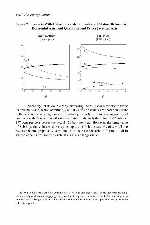
108 / The Energy Journal
35. While this seems quite an extreme stress-test, one can argue that it is justified because long-run elasticity of domestic supply is ignored in this paper. Furthermore, note that a change inq bD
requires also a change in to make sure that the new demand curve still passes through the same�calibration point.
Figure 7. Scenario With Halved Short-Run Elasticity: Relation Between d(Horizontal Axis) and Quantities and Prices (Vertical Axis)
0.2 0.4 0.6 0.8 100
50
100
150
200
250
0.8 10 0.2 0.4 0.60
50
100
150
200
δ δ
qR,1
qR,2
q0
qS
pR,2
pR,1
p0
Δp =p0 – pR,1
(a) Quantities(bcm / year)
(b) Prices(EUR / tcm)
Secondly, let us double by increasing the long-run elasticity to twicekits original value, while keeping .35 The results are shown in Figuree ��0.27SR
8. Because of the very high long-run elasticity, the volume of long-term gas importcontracts with Russia for exceeds quite significantly the actual 2007 volume:d�0197 bcm per year versus the actual 120 bcm per year. However, the large valueof brings the volumes down quite rapidly as increases. As of thek d d�0.5results become graphically very similar to the base scenario in Figure 4. All inall, the conclusions are fairly robust vis-a-vis changes in .k

Russian Gas Imports in Europe / 109
Figure 8. Scenario With Double Long-Run Elasticity: Relation Between d(Horizontal Axis) and Quantities and Prices (Vertical Axis)
0 0.2 0.4 0.6 0.8 10
50
100
150
200
0.2 0.4 0.6 0.8 100
50
100
150
200
250
δ δ
qR,1
qR,2
q0
qS
pR,2
pR,1
p0
Δp =p0 – pR,1
(a) Quantities(bcm / year)
(b) Prices(EUR / tcm)

110 / The Energy Journal