BPEA Conference Draft, September 15–16, 2016

Rules versus discretion: A reconsideration

Narayana Kocherlakota, University of Rochester

Rules versus Discretion: A Reconsideration

Narayana Kocherlakota, University of Rochester and NBER⇤

August 29, 2016

1 Introduction

Over the past forty years, a broad consensus has developed among academic macroeconomists

that policymakers’ choices should closely track pre-determined rules.1 This consensus is

perhaps strongest in monetary economics. It can be traced back to two key papers. From

a theoretical perspective, Kydland and Prescott (1977) showed nominal rigidities created a

challenging time consistency problem for monetary policymakers. Given this problem, it was

welfare-improving to require monetary policymakers to follow a pre-determined rule. From a

practical perspective, Taylor (1993) demonstrated that the Federal Reserve’s monetary policy

choices could, in fact, be well-approximated by a simple feedback rule (from publicly observed

economic conditions to interest rates) and that rule was associated with good macroeconomic

outcomes. These two papers have had enormous influence in both academic and policy circles.

⇤Prepared for Brookings Papers on Economic Activity, Fall 2016. I thank Sam Schulhofer-Wohl and Kei-Mu Yi for their comments. I also thank Alan Blinder, Janice Eberly, and Lars Svensson for their commentson an earlier draft.

1Taylor (1993, p. 197) writes, “If there is anything about which modern macroeconomics is clearhowever - and on which there is substantial consensus - it is that policy rules have major advan-tages over discretion in improving economic performance.” His words go back nearly a quarter cen-tury but are probably now even more widely viewed as being true. Thus, three Nobel Laureates joinedTaylor in signing this letter in support of Congress’ requiring the Fed to explain any deviations fromthe Taylor Rule: http://financialservices.house.gov/uploadedfiles/020916_taylor_letter_with_

signatories_.pdf.Rules enjoy considerably less support among those who actually have the responsibilityof making policy, as evidenced in this open letter from Chair Janet Yellen to Representatives Pelosi andRyan: http://www.federalreserve.gov/foia/files/ryan-pelosi-letter-20151116.pdf.

1

Most academic papers in monetary economics treat policymakers as mere error terms on a

pre-specified feedback rule. Most modern central bank sta↵s model their policymaker bosses

in exactly the same way.

The purpose of the current paper is to re-visit the consensus that favors the use of rules

over discretion in the making of monetary policy. I do so in two ways. The first is empirical.

I use information in the transcripts2 from 2009-10 Federal Open Market Committee (FOMC)

meetings to argue that the FOMC pursued a relatively slow recovery, in which unemployment

was anticipated to take five years to return to its long-run level and inflation was expected

to take even longer to return to the Committee’s long-run target.3 I trace this lack of

aggressiveness to the FOMC’s unwillingness to deviate greatly from the recommendations of

the Taylor Rule4, because it provided a good approximation to the Committee’s pre-2007

policy reaction function.5 I document too that Brunner and Meltzer (1968) arrive at a similar

conclusion about the Great Depression: the Federal Reserve’s poor performance in 1929-30

was attributable to its excessive reliance on its pre-1929 policy framework.

The empirical analysis is a reminder that monetary policymakers are forced to choose

rules based in large part on their past historical performance, and those estimated rules can

give rise to poor outcomes if conditions change su�ciently. However, the analysis leaves open

the possibility that there is some other rule out there, yet to be found, that would dominate

discretion. In the second part of the paper, I explore this question theoretically using the

delegation model of Holmstrom (1984). The main trade-o↵ in the theoretical framework is

that the central bank may desire a di↵erent level of inflation than does society, but the central

2The Federal Open Market Committee publicly releases transcripts of its meetings, along with supportingsta↵ materials, with a five to six year lag. The transcript from the December 2010 meeting is the latest onethat has been released so far.

3I served on the Federal Open Market Committee from October 2009 through October 2015. My commentsabout the FOMC’s policy perspectives in 2009-10 apply with at least as much force to my own during thattime frame.

4The term “Taylor Rule” is used to refer to a wide class of monetary policy rules. Throughout the paper,I use the term to refer specifically to the interest rate rule originally described in Taylor (1993) or to theFOMC sta↵’s version of that rule (which uses Okun’s Law to substitute an unemployment gap for the TaylorRule’s output gap).

5I made a similar argument in Kocherlakota (2015b).

2

bank also has information about the future evolution of inflation that is impossible to write

into a rule. Here, I have in mind that the central bank sees a large number of possible factors,

with time-varying factor loadings, that help it forecast inflation. For example, suppose a large

European financial institution suddenly closes three investment funds.6 How will the central

bank respond to that shock? The appropriate response will depend on a host of details that

would be hard to write into any pre-determined rule.

I compare two possible institutional setups: discretion, under which the central bank

can choose any level of monetary accommodation that it wishes, and a rule, under which

the central bank’s decision is a fixed function of some publicly observable information.7

The benefit of the former institutional framework is that the central bank has the ability

to o↵set shocks that can’t be encoded into a rule, but would otherwise generate highly

variable inflation. The cost of the former framework is that inflationary outcomes will be

systematically di↵erent from the socially optimal level, because of the central bank’s inflation

bias. Correspondingly, I show that, in terms of ex-ante welfare, discretion generates better

outcomes for society as long the central bank has a su�ciently small inflation bias relative

to the magnitude of non-rulable inflationary shocks. (Here, I use two notions of ex-ante

welfare: quadratic loss and a min-max robustness criterion as in Hansen-Sargent (2007).) I

use evidence from the past the past two decades to argue that the Federal Reserve does not

have a material pro-inflation bias (meaning, at most, a quarter percent).8

The empirics and the theory both suggest that, contrary to conventional wisdom, mon-

etary policy rules impede central bank performance. Central banks will achieve better out-

comes if they are given discretion - that is, if on an ongoing basis, they make choices based on

all available information to keep inflation or employment close to target. Importantly, this

recommendation does hinge on the inflationary bias of the central bank being small. That

6Readers will recognize this as a description of BNP Paribas’ decision on August 9, 2007.7My terminology mirrors that in Kydland and Prescott (1977). However, others prefer a broader notion of

rules: what I call discretion in this paper, Bernanke has called a rule: http://blogs.wsj.com/economics/2015/03/02/bernanke-says-fed-already-follows-policy-rule/.

8See Kocherlakota (2015a) for a related discussion.

3

seems to be an accurate description of the Federal Reserve in the past twenty years, but I

provide no guidance about how to ensure that it continues to be true going forward.

My analysis is closely related to much prior work. In terms of the empirics, during the

2009-10 time period, many observers critiqued the FOMC for providing insu�cient levels

of accommodation. My contribution here is that my use of internal Committee documents

(only released over the last couple years) sheds new light on how the FOMC’s pre-crisis

framework contributed to this under-provision of accommodation. In terms of the theory,

Canzoneri (1985) illustrates a similar tension between central bank bias and central bank

private information. Svensson (2003) makes similar points to mine about how discretion

allows central banks to use judgment so as to achieve better macroeconomic outcomes.9

2 The Not-So-Great Recovery and the Taylor Rule

In this section, I discuss the actions of the Federal Open Market Committee (FOMC) during

the beginning of the recovery from the 2007-09 Great Recession. The Committee and its

sta↵ viewed the Taylor Rule as providing a good approximation to the Committee’s pre-2007

reaction function. I argue that, as a result, the FOMC’s choices in 2009-10 were heavily influ-

enced by the prescriptions of that particular rule. I document that this rule-based framework

led the Committee to pursue a relatively slow recovery in both prices and employment. I

briefly parallel the Federal Reserve’s reliance on the Taylor Rule in 2009-10 with the Federal

Reserve’s (considerably more disastrous) reliance on the Riefler-Burgess framework during

the 1929-30 time frame.9Throughout the paper, I compare outcomes under rules to outcomes under complete discretion, so that

the central bank can choose any amount of accommodaiton. In a dynamic version of the problem that Istudy, Athey, Atkeson, and P. Kehoe (2005) prove that the optimal delegation game is either a rule or hasbounded discretion (which is what I term constrained discretion). In their benchmark parametric example,they prove that, as the central bank’s private information becomes increasingly large, the optimal delegationgame converges to one without any constraint on discretion.

4

2.1 The Summary of Economic Projections

My discussion relies heavily on the Summary of Economic Projections (SEP). Beginning

in 2007, FOMC participants (all twelve Presidents of the regional Reserve Banks and the

members of the Federal Reserve’s Board of Governors) have submitted their forecasts for

key macroeconomic variables four times per year. These submissions make up the SEP.

Importantly, as the description of the SEP clearly states, a given participant’s forecast is

“based ... on each participant’s assumptions about factors likely to a↵ect economic outcomes,

including his or her assessment of appropriate monetary policy. ’Appropriate monetary

policy’ is defined as the future path of policy that the participant deems most likely to

foster outcomes for economic activity and inflation that best satisfy his or her interpretation

of the Federal Reserve’s dual objectives of maximum employment and stable prices.” A

given participant’s assessment of the appropriate stance of monetary policy may well di↵er

from their forecast of what the Committee would actually do. As a result, these so-called

projections should not be seen as reflecting participants’ forecasts for the actual course of

the economy. Rather, beyond the usual one to two year lag associated with monetary policy,

a participant’s projection is best viewed as a description of his or her monetary policy goals

for the evolution of the relevant macroeconomic variables.

After the relevant meeting, the FOMC releases summary statistics from the SEP to the

public. However, when the FOMC releases the meeting transcript (five plus years later), it

also releases the full set of SEP submissions. The full SEPs provide valuable information,

as they link participants’ relatively detailed and standardized assessments of the economy

and policy with their forecasts.10 I exploit all of this public information heavily. Hence, my

discussion will focus on the SEP from the years 2009-10, since the full SEP from later years

have not been released. As well, I restrict attention to the fourth quarter SEPs from those

years because they have a longer forecast horizon than SEPs from earlier in the year.

10Unfortunately, the submissions remain anonymous for another five years. As a result, it is impossible tolink a participant’s submissions at one meeting to his/her submissions at another until a decade after bothmeetings.

5

2.2 The FOMC’s Limited Ambitions

According to the Federal Reserve Act, the FOMC is charged by Congress to make monetary

policy so as to promote price stability and maximum employment. The Committee has

translated the former objective into a goal of 2% for Personal Consumption Expenditure

(PCE) inflation. In terms of the latter objective, it tracks progress using a number of metrics,

but tends to put the most weight on the unemployment rate. In principle, the two mandated

objectives could conflict with one another, and that conflict did shape the SEP submissions

of some participants. However, most saw no conflict between the two goals during this time

frame between the two mandates: inflation was expected to be too low and unemployment

was expected to be too high.

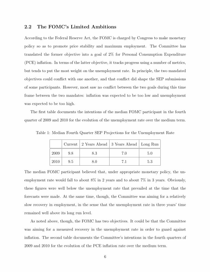
The first table documents the intentions of the median FOMC participant in the fourth

quarter of 2009 and 2010 for the evolution of the unemployment rate over the medium term.

Table 1: Median Fourth Quarter SEP Projections for the Unemployment Rate

Current 2 Years Ahead 3 Years Ahead Long Run

2009 9.8 8.3 7.0 5.0

2010 9.5 8.0 7.1 5.3

The median FOMC participant believed that, under appropriate monetary policy, the un-

employment rate would fall to about 8% in 2 years and to about 7% in 3 years. Obviously,

these figures were well below the unemployment rate that prevailed at the time that the

forecasts were made. At the same time, though, the Committee was aiming for a relatively

slow recovery in employment, in the sense that the unemployment rate in three years’ time

remained well above its long run level.

As noted above, though, the FOMC has two objectives. It could be that the Committee

was aiming for a measured recovery in the unemployment rate in order to guard against

inflation. The second table documents the Committee’s intentions in the fourth quarters of

2009 and 2010 for the evolution of the PCE inflation rate over the medium term.

6

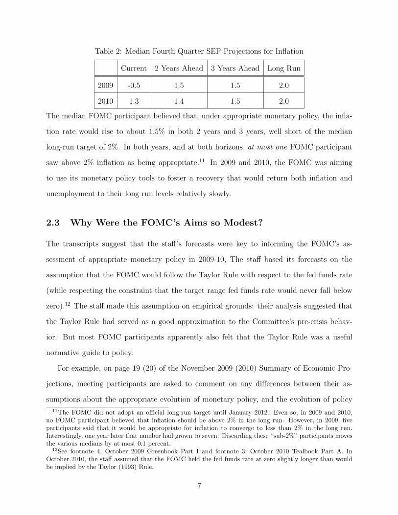
Table 2: Median Fourth Quarter SEP Projections for Inflation

Current 2 Years Ahead 3 Years Ahead Long Run

2009 -0.5 1.5 1.5 2.0

2010 1.3 1.4 1.5 2.0

The median FOMC participant believed that, under appropriate monetary policy, the infla-

tion rate would rise to about 1.5% in both 2 years and 3 years, well short of the median

long-run target of 2%. In both years, and at both horizons, at most one FOMC participant

saw above 2% inflation as being appropriate.11 In 2009 and 2010, the FOMC was aiming

to use its monetary policy tools to foster a recovery that would return both inflation and

unemployment to their long run levels relatively slowly.

2.3 Why Were the FOMC’s Aims so Modest?

The transcripts suggest that the sta↵’s forecasts were key to informing the FOMC’s as-

sessment of appropriate monetary policy in 2009-10, The sta↵ based its forecasts on the

assumption that the FOMC would follow the Taylor Rule with respect to the fed funds rate

(while respecting the constraint that the target range fed funds rate would never fall below

zero).12 The sta↵ made this assumption on empirical grounds: their analysis suggested that

the Taylor Rule had served as a good approximation to the Committee’s pre-crisis behav-

ior. But most FOMC participants apparently also felt that the Taylor Rule was a useful

normative guide to policy.

For example, on page 19 (20) of the November 2009 (2010) Summary of Economic Pro-

jections, meeting participants are asked to comment on any di↵erences between their as-

sumptions about the appropriate evolution of monetary policy, and the evolution of policy

11The FOMC did not adopt an o�cial long-run target until January 2012. Even so, in 2009 and 2010,no FOMC participant believed that inflation should be above 2% in the long run. However, in 2009, fiveparticipants said that it would be appropriate for inflation to converge to less than 2% in the long run.Interestingly, one year later that number had grown to seven. Discarding these “sub-2%” participants movesthe various medians by at most 0.1 percent.

12See footnote 4, October 2009 Greenbook Part I and footnote 3, October 2010 Tealbook Part A. InOctober 2010, the sta↵ assumed that the FOMC held the fed funds rate at zero slightly longer than wouldbe implied by the Taylor (1993) Rule.

7

assumed by sta↵ (the Taylor Rule). Several participants did project that, under appropri-

ate monetary policy, the fed funds rate should rise more rapidly than the sta↵ expected.13

However, these participants largely trace their preference for higher interest rates to their

expectations that inflation would rise more rapidly than anticipated by sta↵. They don’t say

that they favor a di↵erent rule, in the sense that they would prefer a di↵erent fed funds rate

target, conditional on the same inflation and unemployment rate realizations.14

This suggests that FOMC participants viewed the Taylor Rule - the Committee’s pre-

crisis reaction function - as being a key guide to their policy choices during the early part of

the economic recovery. We can see how this reliance on the Taylor Rule a↵ected the FOMC’s

medium-term macroeconomic goals by looking at the sta↵’s long-term outlook (which was

based on the Taylor Rule) in the fourth quarters of 2009 and 2010.

13No participant in either November 2009 or November 2010 pointed to a more gradual increase as beingappropriate.

14In November 2009, a couple participants (5 and 16) stated in their SEP submissions that they favoreda higher fed funds rate than implied by the Taylor Rule because they felt that historically low interest ratescould lead to imbalances and undue risk-taking. No participant in either the November 2009 or November2010 meetings specifically favored a lower interest rate path than that described by the Taylor Rule. (I shouldnote that a key shortcoming of the 2009-10 SEPs is that participants did not submit quantitative forecastsfor the evolution of the fed funds rate.)

It may be surprising that more participants did not mention financial stability concerns as a reason totighten policy faster than recommended by the Taylor Rule. It’s important to keep in mind that I’m discussinga period in which the unemployment rate was generally well above 9%. It was hard to see any signs of“overheating” or “froth” in financial markets. Much of the Committee’s discussion was about the magnitudeof the downward pressures on inflation generated by economic slack. (See December 2009 FOMC meeting fora particularly thorough sta↵ briefing along these lines.) The situation was quite di↵erent in, say, mid-2013when the FOMC publicly began to discuss its plans for tapering asset purchases.

8

Table 3: FOMC Sta↵’s Projections

2009:IV proj. for UR 2009:IV proj. for core ⇡ 2010:IV proj. for UR 2010:IV proj. for core ⇡

2010:IV 9.5 1.1 9.7 1.1

2011:IV 8.2 1.0 9.0 1.0

2012:IV 6.1 1.1 7.9 1.0

2013:IV 4.9 1.4 7.1 1.2

2014:IV 4.7 1.6 6.1 1.3

2015:IV NA NA 5.2 1.5

This outlook features a slow decline in the unemployment rate, coupled with an even

slower increase in the inflation rate (back to, in this case, the sta↵’s assumed target of 2%).

While there are di↵erences (notably with the 3-year-ahead unemployment forecast in 2009),

this sta↵ outlook is broadly similar to the median projections of the FOMC participants.

This similarity is consistent with the perspective that the FOMC saw a slow recovery in

unemployment and inflation as being appropriate because the Taylor (1993) Rule - a good

approximation to the FOMC’s pre-crisis reaction function - implied that kind of slow recovery.

Why did the Taylor Rule imply such a slow recovery? The Taylor Rule is designed

to eliminate gaps between inflation gaps (between current inflation and a 2% target) and

output/unemployment gaps. However, the Rule constrains the size of the FOMC’s response

to these gaps; in particular, it precludes the FOMC from rapidly cutting interest rates until all

gaps are eliminated.15 In this sense, the Taylor Rule represents a constraint on the FOMC’s

interest rate response to inflation and activity gaps.

Mathematically, we can think of the Taylor Rule as putting weight on an implicit objective

of keeping the fed funds rate close to its historically normal level. To be more concrete,

suppose that the central bank has a quadratic loss function with weight on both inflation gaps

15Here, I assume (as is true in New Keynesian models among others) that the FOMC’s current interest ratechoices have some e↵ect on current outcomes. In contrast, Svensson (1997) assumes that current monetarypolicy choices have no impact on macroeconomic outcomes for two years.

9

and interest rate gaps. Suppose as well that the current inflation rate is (well-approximated

by) an a�ne function of the current interest rate. Then the bank’s optimal interest rate

choice would set the interest rate equal to an a�ne function of the inflation gap. It is readily

shown that the slope in this relationship converges to infinity as the weight in the objective

on interest rate gaps converges to zero.

2.4 Could the FOMC Have Done Anything Di↵erently?

As of November 2009, the FOMC had already lowered the target range for the fed funds

rate to near zero and had bought a large amount of long-term assets. What else could the

Committee have possibly done to stimulate inflation and employment? The sta↵ analysis at

the time suggested two answers to this question: asset purchases and forward guidance. The

two answers are conceptually quite di↵erent. By buying longer-term assets, the Committee

intended to push up their price and incentivize spending on the part of those who would

normally hold those longer-term assets. Through forward guidance, the Committee intended

to change private sector beliefs about the future course of short-term interest rates - that is,

about the likely pace of the removal of accommodation. I’ll discuss each of these tools in

turn.

2.4.1 Asset Purchases

The FOMC relied heavily on long-term asset purchases as a form of monetary stimulus

during the recovery. The sta↵ regularly presented possible options to the Committee that

featured more aggressive use of this tool. For example, in November 2009, the sta↵ presented

a policy option to the FOMC according to which the Committee would have lengthened the

duration of an ongoing asset purchase program. The sta↵ argued that doing so would allow

the FOMC to accelerate the economy’s return to full employment, guard against downside

risks, and raise unduly low inflation. No participant spoke in support of this policy option.16

16From October 2009 Bluebook, p. 41: “The Committee may view the sta↵’s economic outlook, with itsvery protracted return to full employment, as producing unacceptably poor outcomes given the Committee’s

10

After the November 2010 meeting, the FOMC announced that it would purchase $600

billion of long-term assets in a policy action that became known as QE2 (to refer to a second

round of “quantitative easing”). However, within the meeting, sta↵ presented a policy option

under which the Committee would have bought $1 trillion of long-term assets. Again, they

argued that this step would allow the Committee to accelerate the pace of the recovery in

both inflation and employment. No participant supported this policy option.17

There were a number of reasons behind the Committee’s reluctance to undertake a larger

asset purchase program. In a non-routine October 2010 FOMC meeting about potential

forms of additional accommodation, I pointed out that the theoretical literature o↵ered little

support for the use of asset purchases as way to provide accommodation.18 I also suggested

five immediate risks associated with the use of asset purchases:19

• There was likely to be huge market uncertainty about the eventual stock of our pur-

chases (which, according to the FOMC, was what mattered for the stimulus).

• Other large holders of long-term Treasuries could o↵set the FOMC’s policy action by

dual mandate. Or participants might believe there remains a non-negligible risk that the economy could su↵era relapse and fall back into recession next year when some of the lending facilities and other governmentprograms wind down. Policymakers may also be troubled by continued inflation readings well below theinflation objectives implicit in the majority of their longer-run projections. For these reasons, they mayjudge that additional monetary stimulus would be appropriate. The Committee might conclude that ane↵ective way to provide such stimulus would be to expand the amount of agency MBS purchases and toextend the timeframe for conducting agency MBS and agency debt transactions (thereby allowing a higheramount of agency debt to be bought without causing market disruption).”

17From October 2010 Tealbook B, p. 18: “Policymakers may believe that without fairly aggressive policyaction soon, both employment and inflation will likely be below the Committee’s objectives for these variablesfor a very substantial period. Moreover, they may be worried that very low inflation poses significant risksto the recovery. If so, the Committee may wish to provide more substantial policy accommodation at thismeeting, as in Alternative A [which involved purchasing $1 trillion of long-term assets, rather than $600billion]. Committee members may, like the sta↵, expect the economic recovery to remain quite gradual, evenwith the additional $600 billion expansion of the Federal Reserve’s balance sheet envisioned in AlternativeB. In the sta↵’s baseline projection, the unemployment rate does not fall below 9 percent until 2012, andinflation remains below levels that the Committee sees as consistent with its objectives for much longer.Members may see such outcomes as unacceptable.”

18See pp. 19-22 of the October 2010 FOMC transcript. I focus on my own remarks for what shouldbe obvious reasons. I was certainly not the only participant at the meeting to express concerns about thedownside risks aassociated with asset purchases.

19I certainly wasn’t alone in seeing risks associated with asset purchases. In December 2009, ChairmanBen Bernanke expressed his concern that additional asset purchases could destabilize inflation expectationsor lead to undesirably sharp upward movements in commodity prices. Arguably, the latter actually did cometo pass in the first half of 2011 after the FOMC launched QE2.

11

markedly reducing their positions.

• There could be an untoward response in the value of the dollar relative to other cur-

rencies.

• If the Federal Reserve’s balance sheet ever grew to be $3 trillion to $4 trillion in size,

the FOMC might not have the tools necessary to raise rates when desired.

• The Fed is taking duration risk onto the balance sheet of taxpayers. They might not

be too pleased about the Fed’s doing so.

I would say that, six years later, the risks that I mentioned have largely proven to be manage-

able or insubstantial. (The last issue seems still up in the air.) But I would still argue that,

as of late 2010, the downsides of asset purchases seemed large when the baseline economic

theory suggested their upside was near zero.20

2.4.2 Forward Guidance

The second tool available to the FOMC, forward guidance, had a much stronger theoreti-

cal basis and represented (as I said at the same October 2010 FOMC meeting) a relatively

low-risk alternative to asset purchases. Throughout the November 2009-November 2010 time

frame, the Committee provided a qualitative form of forward guidance, saying that it antic-

ipated that the fed funds rate would remain extraordinarily low for “an extended period.”

As William Dudley, vice-chair of the FOMC noted, this phrase was widely understood as

meaning that “no tightening was likely for more than six months.”21 The Committee was

20The baseline economic theory that I have in mind is Eggertsson and Woodford (2003), which builds onthe work of Wallace (1981). In these papers, through a Ricardian Equivalence argument, long-term assetpurchases have no impact on long-term yields. There is much empirical work based on central bank assetpurchase programs (both here and elsewhere) that suggests that, in fact, the purchases did lead to a declinein long-term yields. As Woodford (2012) points out, it is a distinct question whether this decline in long-term yields was associated with an increase in economic activity. I would guardedly endorse Bernanke’s(2012) conclusion that, “Overall, however, a balanced reading of the evidence supports the conclusion thatcentral bank securities purchases have provided meaningful support to the economic recovery while mitigatingdeflationary risks.”

21November 2009 FOMC transcript, p. 168. See also the results of the primary dealer survey reported onp. 5 of December 2009 transcript.

12

concerned throughout this period that this forward guidance would be regarded as a com-

mitment, while it was only meant as a forecast.22

In November 2010, sta↵ presented a policy option under which the FOMC would adopt a

stronger form of forward guidance (along with the larger $1 trillion asset purchase program

noted above). According to this guidance, the FOMC would state that it intended to keep

the fed funds rate extraordinarily low until mid-2012. The proposed guidance came with a

number of escape clauses, designed to prepare the public for the possibility that the FOMC

might raise the fed funds rate more rapidly. No one at the meeting spoke in favor of this

more specific form of forward guidance.

Actually, the sta↵’s analysis at the two November meetings supported the adoption of

much more aggressive forms of forward guidance. The sta↵ routinely provided forecasts of

the optimal path of fed funds rate target choices that were based on the benchmark FRB-US

model.23 In both November 2009 and November 2010, these optimal control exercises resulted

in interest rate paths that stayed at a quarter percent until the unemployment rate fell to

about 5%.24 This delay in the initation of interest rate increases provides considerably more

monetary accommodation than results from following the recommendations of the Taylor

Rule.

Interestingly, these 2009-10 optimal control prescriptions are both relatively close to what

the FOMC actually ended up doing: it did not raise the fed funds rate target range from its

2008 level until the unemployment rate was 5%. But the policy is much more stimulative in

the model because people know well in advance that the Fed intends to keep interest rates

low until the unemployment rate hits 5%. They did not have that knowledge in the real

22See, for example, Bernanke, p. 119 of March 2010 FOMC transcript: “. . . this is clearly not a fixed timecommitment. It is a conditional statement . . . . I would just ask ... that everybody emphasize in talkingabout this publicly that it is conditional and that we are tying our policy to the state of the economy.”

23The term “optimal” refers to minimizing a loss function that puts equal weight on squared deviations ofinflation from 2%, squared deviations of the unemployment rate from the natural rate, and squared interestrate changes. The last term is motivated by the sta↵’s desire to capture the FOMC’s apparent aversionto interest rate changes. See Svensson and Tetlow (2005) for an extensive analysis of the optimal policyprojections made by FOMC sta↵.

24This is a description of the relevant graphs on p. 25 of the November 2009 Bluebook and p. 3 of Part Bof the November 2010 Tealbook.

13

world: In late 2009, Blue Chip forecasters expected that the FOMC would first raise interest

rates when the unemployment rate was near 10%.25

Over two years later, in December 2012, the FOMC implemented a new kind of forward

guidance that committed to keeping the fed funds rate extraordinarily low at least as long

as the unemployment rate stayed above a particular numerical threshold (and as long as

inflation and inflation expectations stayed under control). The sta↵ analysis available at the

November 2009 and 2010 meetings suggests that their forecasts for both unemployment and

inflation would have been considerably more optimistic had the FOMC chosen to implement

an aggressive form of threshold-based forward guidance at either of those meetings. More

specifically, suppose that the FOMC had announced sometime in 2010 that its intention was

to keep the fed funds rate extraordinarily low at least until the unemployment rate reached

5% (as long as inflation and inflation expectations stayed under control). According to the

sta↵’s optimal control exercises in late 2009 and in late 2010, this aggressive forward guidance

would have brought the unemployment rate back to pre-crisis levels about one year earlier

than under the sta↵’s benchmark outlook, while the inflation rate would have returned to

target within the forecast horizon.26 To the extent that one views asset purchases as being

stimulative, this forecast underestimates what the FOMC could have expected to achieve

using its tools.27

25Bernanke (2012, fn. 25). This timing of the removal of accommdation is much earlier than is implied bythe Taylor Rule.

26Like the sta↵’s baseline FRB-US model, this comparison abstracts from the possibility that a fasterrecovery would have had permanent positive e↵ects on the long-run level of economic activity. ChairmanBen Bernanke discusses this benefit of additional stimulus in some detail on page 99 of the November 2010transcript.

27There is another, more subtle, reason why the forecast underestimates what the FOMC could achievein terms of unemployment and inflation. In the optimal control exercise, the sta↵ uses a loss function thatputs substantial weight on interest rate changes. That loss function leads the FOMC to begin to raise ratestoo early and too slowly, relative to the optimal path under a loss function that doesn’t put any weight oninterest rate changes.

14

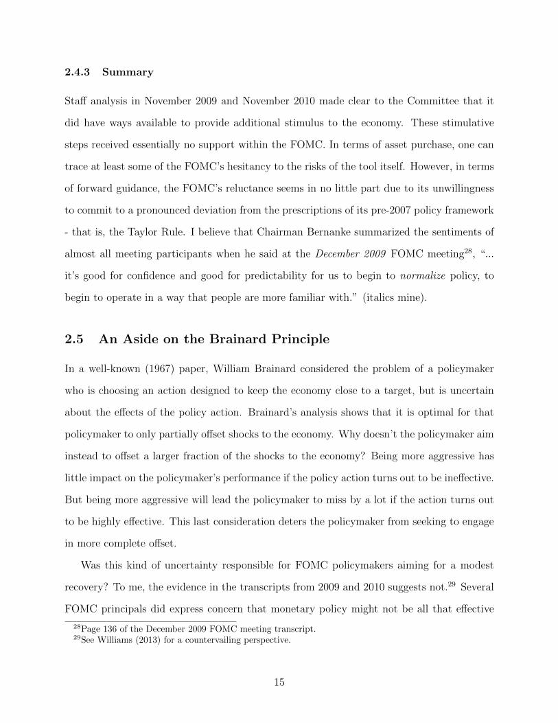
2.4.3 Summary

Sta↵ analysis in November 2009 and November 2010 made clear to the Committee that it

did have ways available to provide additional stimulus to the economy. These stimulative

steps received essentially no support within the FOMC. In terms of asset purchase, one can

trace at least some of the FOMC’s hesitancy to the risks of the tool itself. However, in terms

of forward guidance, the FOMC’s reluctance seems in no little part due to its unwillingness

to commit to a pronounced deviation from the prescriptions of its pre-2007 policy framework

- that is, the Taylor Rule. I believe that Chairman Bernanke summarized the sentiments of

almost all meeting participants when he said at the December 2009 FOMC meeting28, “...

it’s good for confidence and good for predictability for us to begin to normalize policy, to

begin to operate in a way that people are more familiar with.” (italics mine).

2.5 An Aside on the Brainard Principle

In a well-known (1967) paper, William Brainard considered the problem of a policymaker

who is choosing an action designed to keep the economy close to a target, but is uncertain

about the e↵ects of the policy action. Brainard’s analysis shows that it is optimal for that

policymaker to only partially o↵set shocks to the economy. Why doesn’t the policymaker aim

instead to o↵set a larger fraction of the shocks to the economy? Being more aggressive has

little impact on the policymaker’s performance if the policy action turns out to be ine↵ective.

But being more aggressive will lead the policymaker to miss by a lot if the action turns out

to be highly e↵ective. This last consideration deters the policymaker from seeking to engage

in more complete o↵set.

Was this kind of uncertainty responsible for FOMC policymakers aiming for a modest

recovery? To me, the evidence in the transcripts from 2009 and 2010 suggests not.29 Several

FOMC principals did express concern that monetary policy might not be all that e↵ective

28Page 136 of the December 2009 FOMC meeting transcript.29See Williams (2013) for a countervailing perspective.

15

relative to historical norms (and I say as much above when I discuss asset purchases). In

light of this risk, Brainard’s results imply that it would have been appropriate for the FOMC

to undershoot its inflation and employment objectives. However, Brainard’s analysis also

implies that the risk of policy ine↵ectiveness should have led Committee members to favor

unusually high levels of accommodation (just not high enough to hit inflation and employment

targets). But, as we have seen, the Committee was loath (during this period) to adopt a

more accommodative stance than the historically based prescriptions of the Taylor Rule.

2.6 An Analogy: The Fed’s Great Depression Policy Error

In this subsection, I briefly recapitulate Brunner and Meltzer’s classic (1968) analysis of

the Federal Reserve’s policy error during the early part of the Great Depression. My basic

point is that, just as in 2009-10, the Federal Reserve’s decision-making in 1929-30 was overly

influenced by its pre-downturn decision framework. (To be clear, the the policy error in

1929-30 led to a macroeconomic catastrophe compared to what happened in 2009-10 and

thereafter.)

Brunner and Meltzer argue that, during the 1920s, the Federal Reserve developed a

framework to guide its decision-making about monetary policy that was sketched in the Board

of Governors’ tenth annual report (for the year 1923). A core element of this framework is

that the presumption that banks only borrowed reserves from the Fed when they needed

those reserves to meet large deposit outflows. This presumption allowed policymakers to use

borrowed reserves as a signal about the relative tightness of monetary policy. High amounts

of borrowed reserves, especially if interest rates were high, signaled that money demand

was high relative to supply, and the stance of policy was tight. Low amounts of borrowed

reserves, especially if interest rates were low, signaled that money demand was low relative to

supply, and the stance of policy was easy. In his magisterial history of the Federal Reserve,

Meltzer summarizes this framework as saying that “if borrowing and interest rates were low,

16

policy was easy; if the two were high, policy was tight.”30 Brunner and Meltzer refer to this

framework as the Riefler-Burgess doctrine, in honor of two Federal Reserve sta↵ economists31

who played a key role in its development.32

Brunner and Meltzer argue that Federal Reserve decision-makers turned to the Riefler-

Burgess doctrine during the early part of the Depression to help guide their thinking about

monetary policy. For example, toward the end of 1930, member bank borrowing from the

Federal Reserve was low relative to historical norms, even though interest rates were also

unusually low. These metrics led many Reserve Bank leaders to conclude that monetary

policy was easy - so easy, that in September 1930, the Federal Reserve strongly considered

selling securities as a way to tighten monetary policy during a period of rampant deflation.

Meltzer (2003) summarizes the Federal Reserve’s thinking in the 1929-30 period as follows,

“People see most clearly what they are trained or disposed to see. The Riefler-Burgess ...

doctrine ... was not a mechanical formula directing Federal Reserve policy, but it directed

attention to member bank borrowing and market interest rates as measures of tightness

and ease. In 1929-30, most members of the Federal Reserve Board and governors of the

reserve banks accepted this framework. They believed that they had acted decisively to ease

credit conditions, and on their measures they had.”33 This description, with the obvious

substitutions, seems apt for the 2009-10 period as well.

3 Modeling Rules versus Discretion

In the preceding section, I described how the FOMC could have achieved its inflation and

employment objectives more rapidly if it had been willing to deviate more from its pre-crisis

reaction function, as proxied by the Taylor Rule. Of course, the Taylor Rule is only one

30Meltzer (2003, p. 164).31More specifically, Winfield Riefler (a Board sta↵ economist) and W. Randolph Burgess (a Federal Reserve

Bank of New York sta↵ economist)32Meltzer (2003, p. 161) notes that Benjamin Strong, the first governor of the Federal Reserve Bank of

New York, also contributed to the development of the Riefler-Burgess framework.33Meltzer (2003, p. 403).

17

possible rule. In this section, I describe a simple model that will allow for a more general

comparison of central bank discretion with central bank rules.

3.1 Environment

Consider the following three stage environment, in which the stages are indexed 0, 1, 2. In

the final stage 2, inflation ⇡ is realized. It is the sum of four components:

⇡ = xR + xNR + a+ "

The first component (xR) is a signal that is revealed at the beginning of the intermediate

stage 1 that is rulable - that is, it can be encoded into a policy rule. The second component

(xNR) is a signal that is observed (at least by the central bank and possibly to others) at

the beginning of stage 1, but is non-rulable (cannot be written into a rule). The third

component (a) is the level of accommodation determined by the central bank in stage 1. The

final component (") is a random shock to inflation that is realized in stage 2.

It is common knowledge in stage 0 that the continuous density of x, over its support

XR, is given by g. For now, I will assume that it is also common knowledge in stage 0

that, conditional on xR, (xNR, ") are mutually independent mean zero random variables with

respective supports XNR and E. Their respective continuous densities, conditional on xR,

are represented by f(.|xR) and h(.|xR). I assume that (XR, XNR, E) are all intervals in the

real line.

The objective function of the central bank is defined over inflation and is known to be:

�(⇡ � ⇡CB)2

The objective function of society over inflation is known to be:

�(⇡ � ⇡SOC)2

18

These objective functions allow for the possibility that the central bank’s inflation target ⇡CB

is distinct from that society’s inflation target ⇡SOC .

3.2 Interpretation of the Environment

There are three main attributes of the environment. The first is that the central bank

has information xNR available that is useful in forecasting inflation, but cannot be used as

the basis of a policy rule. The idea behind y being non-rulable is that it is a complicated

function of possibly many time-varying factors on inflation (thus, xNR = ✓

0�, where ✓ and �

are both very long vectors). This emphasis on the importance of non-rulable information is

consistent with the fact that most central banks base their inflation forecasts on objects like

potential output and the natural rate of interest that are complex functions of observable

and unobservable data (like sta↵ judgments of various kinds). I view this modeling as being

a simple way to formalize Svensson (2003)’s observation that “central banks have developed

very elaborate and complex decision-making processes, where large amounts of information

are collected, processed, and analyzed, and where considerable judgment is exercised.”

The second is that the central bank’s objective for inflation could di↵er from that of

society’s. There are many possible reasons for this bias, like political economy e↵ects of

various kinds. However, it could simply be that the central bank’s horizon is short-run, while

society’s is long-run. In this way, the model can capture the e↵ects of time inconsistency.34

The final attribute of import is that society has no way to o↵er outcome-contingent

rewards or punishments to the central banker. In elegant work, Walsh (1995) showed how

such rewards/punishments can be used to align a central banker’s incentives with society’s.

However, it does seem challenging to implement such schemes in reality (at least in the US).

34To be a little more precise: this one-period model is meant to capture the central bank’s decision problemafter the private sector has made its decisions that feed into inflation within the current period. This timingmeans that the central bank’s objective in this decision problem does not include the impact of its reactionfunction on the private sector’s expectations - exactly the time consistency problem highlighted originally byKydland and Prescott (1977).

19

3.3 Delegation Games

My results are about delegation games, in which the central bank can directly choose the level

of accommodation from a set of possibilities. In this subsection, I show that any equilibrium

outcome of any game played by the central bank in this environment is an equilibrium

outcome of a delegation game.

I define a game to be a pair (C,↵). Here, the first component C is a correspondence from

the set XR of realizations of the rulable signal into some set � of actions for the central

bank. The game component ↵ is a continuous outcome function that maps (� ⇥ XR) into

the real line; given the rulable signal, it describes the accommodation resulting from the

central bank’s choice of �. The set of equilibria EQM(C,↵) to the game (C,↵) consists of all

functions �⇤ : XR ⇥XNR ! � such that �⇤ is the central bank’s best response as a function

of the rulable and non-rulable signals (xR, xNR) about inflation:

�

⇤(xR, xNR) 2 argmax�✏C(xR) �ˆ"2E

(↵(�, xR) + xR + xNR + "� ⇡SOC)2h("|xR)d"

I define a delegation game to be a game (C,↵) in which the range � of the correspondence

C is a subset of the real line and the outcome function ↵(�, xR) = �. In a delegation game,

the central bank directly chooses an accommodation level from a set of possibilities that can

vary with the rulable information xR.

The following proposition shows that there is no loss in generality in restricting attention

to the equilibrium outcomes of delegation games.

Proposition 1. Consider a game (C,↵) in which �

⇤ 2 EQM(C,↵). Then, let �0 = [xR2XR[xNR2XNR

20

↵(�⇤(xR, xNR), xR). Define the delegation game (C’,↵0) by

C

0(xR) = [x0NR✏Y ↵(�

⇤(xR, x0NR), xR)

↵

0(�, xR) = �

Then �

0 is an equilibrium to (C 0,↵

0), where:

�

0(xR, xNR) = ↵(�⇤(xR, xNR), xR) 8(xR, xNR) 2 (XR ⇥XNR)

Proof. For any xR in XR and any xNR in XNR, we know that �

⇤(xR, xNR) 2 C(xR). If

the central bank observes rulable information xR and non-rulable information xNR, then the

central bank weakly prefers the action �

⇤(xR, xNR) to the action �

⇤(xR, x0NR) for any x

0NR,

so that for any (xR, xNR, x0NR) :

�ˆ"2E

(xR + xNR + "+ ↵(�⇤(xR, xNR), xR)� ⇡SOC)2h("|xR)d"

� �ˆ"2E

(xR + xNR + "+ ↵(�⇤(xR, x0NR), xR)� ⇡SOC)

2h("|xR)d"

This inequality implies that for any (xR, xNR, x0NR) :

�ˆ"2E

(xR + xNR + "+ ↵

0(�0(xR, xNR), xR)� ⇡SOC)2h("|xR)d"

� �ˆ"2E

(xR + xNR + "+ ↵

0(�0(xR, x0NR), xR)� ⇡SOC)

2h("|xR)d"

Equivalently:

�ˆ"2E

(xR + xNR + "+ ↵

0(�0(xR, xNR), xR)� ⇡SOC)2h("|xR)d"

= max�2C0(xR) �ˆ"2E

(xR + xNR + "+ ↵

0(�, xR)� ⇡SOC)2h("|xR)d"

This proves the proposition’s claim that �0 is an equilibrium to the delegation game (C 0,↵

0).

21

Proposition 1 is, essentially, an application of the revelation principle in this setting. In

keeping with Proposition 1, I will focus on delegation games in the remainder of the paper.

I will pose the rules versus discretion question as being about the nature of the restrictions

embedded in the correspondence C.

3.4 Kinds of Delegation Games

In light of Proposition 1, we can restrict attention to delegation games. There are three

possible kinds of delegation games. The first kind are rules that restrict the central bank’s

choice to depend only on the rulable information xR about future inflation.

Definition 1. Suppose (C,↵) is a delegation game. The game is said to be a rule if C(xR)

is a singleton for almost all xR in XR.

In a rule, the public knows exactly what the central bank will do as a function of the

rulable variable xR

The second kind of delegation game features discretion, in the sense that the central bank

is always allowed to choose any level of accommodation.

Definition 2. Suppose (C,↵) is a delegation game. The game is said to feature discretion

if C(xR) is the entire real line for almost all xR in XR.

All other delegation games are said to feature constrained discretion.

Definition 3. Suppose (C,↵) is a delegation game. The game is said to feature constrained

discretion if, for some set of xR in XR that has positive measure, C(xR) is a proper subset of

the real line and if, for some set of x0R 2 XR with positive measure, C(x0

R) is not a singleton.

I will largely be interested in comparing outcomes under rules with outcomes under games

that feature discretion. The following result will help in that investigation. Define the stage 0

22

social welfare associated with any rule (C,↵) to be the expected value of the social planner’s

objective implied by that rule:

�ˆxR2XR

ˆxNR2XNR

ˆ"2E

(xR + xNR +C(xR) + "� ⇡SOC)2h("|xR)f(xNR|xR)g(xR)d"dxNRdxR

Proposition 2. Consider the rule (C⇤,↵) such that C⇤(xR) = ⇡SOC � xR for any xR 2 XR.

No other rule has higher stage 0 social welfare.

Proof. Rewrite the stage 0 welfare associated with a rule (C,↵) as:

�ˆxR2XR

ˆxNR2XNR

ˆ"2E

[(xR + C(xR)� ⇡SOC)2 + (xNR + ")2]h("|xR)f(xNR|xR)g(xR)d"dxNRdxR

�2

ˆxR2XR

ˆxNR2XNR

ˆ"2E

(xR + C(xR)� ⇡SOC)(xNR + ")h("|xR)f(xNR|xR)g(xR)d"dxNRdxR

Recall that:

ˆxNR2XNR

ˆ"2E

(xNR + ")h("|xR)f(xNR|xR)d"dxNR = 0 for all xR in X

Hence, the stage 0 welfare can be expressed as:

�ˆxR2XR

(xR + C(xR)� ⇡SOC)2g(xR)dxR

�ˆxR2XR

ˆxNR2XNR

ˆ"2E

(xNR + ")2h("|xR)f(xNR|xR)g(xR)d"dxNRdxR

and this expression is maximized by setting the first integrand to zero - that is, setting

C(xR) = ⇡SOC � xR.

The best rule is to o↵set the inflationary pressures embedded in the rulable signal xR.

23

This rule provides stage 0 social welfare equal to:

V

optrule = �

ˆxR2XR

ˆxNR2XNR

ˆ"2E

(xNR + ")2h("|xR)f(xNR|xR)g(xR)d"dxNRdxR

=�ˆxR2XR

ˆxNR2XNR

x

2NRf(xNR|xR)g(xNR)dxNRdxR �

ˆxR2XR

ˆ"2E

"

2h("|xR)g(xR)d"dxR

=� V ar(xNR)� V ar(")

Here, I use the notation V ar(.) to refer to the variance of the relevant random variable, as

of stage 0. The stage 0 social welfare is the negative of the sum of two components: the

variance of the non-rulable inflation shock xNR and the variance of the ex-post inflationary

shock ".

4 Main Theoretical Results

We can now use the theoretical model described in the prior section to assess whether rules

are superior to discretion, or vice-versa. The answers to this question generally trade o↵ two

quantities: the magnitude of central bank bias versus the variance reduction gains associated

with allowing the central bank to o↵set shocks to inflation that are hard to encode in rules.

Suppose first that there is no non-rulable information and no inflation bias. Then, dis-

cretion is equivalent to the best possible rule.

Proposition 3. Suppose XNR = {0}, so that there is no non-rulable information, and

⇡CB = ⇡SOC , so that the central bank is unbiased. There is a unique equilibrium outcome

to any delegation game with discretion and its stage 0 social welfare is equal to the stage 0

social welfare implied by the best possible rule.

Proof. Consider any delegation game (C,↵). Then, in stage 1, the central bank solves the

problem:

maxa2C(xR) �ˆ"2E

(xR + "+ a� ⇡SOC)2h("|xR)d"

24

which can be rewritten as:

maxa2C(xR)[�ˆ"2E

"

2h("|xR)d"� (xR + a� ⇡SOC)

2]

Suppose the delegation game features discretion, so that C(xR) is the entire real line. Then

the unique solution to this problem would be to set:

a = ⇡SOC � xR.

The stage 0 welfare associated with this equilibrium is easily seen to be V

optrule.

The proposition demonstrates that, without any non-rulable information or bias, the best

rule is equivalent to discretion.

At this point, it is worth noting something obvious that is often ignored. Many economists

will airily say that, “Rules are better than discretion.” The above proposition makes clear

how sloppy this language is. In the context without bias or non-rulable information, any rule

other than the best one provides less stage 0 welfare. Hence, it is not true that rules are as

good as discretion. What’s true is that there is exactly one (carefully chosen) rule that does

as well as discretion.

Suppose next that the central bank’s information about inflation is all rulable and and

that the central bank is biased. Then, discretion is worse in terms of stage 0 welfare than

the best possible rule.

Proposition 4. Suppose XNR = {0}, so that all available information about inflation is

rulable, and ⇡CB 6= ⇡SOC , so that the central bank has an inflation bias. There is a unique

equilibrium outcome to any delegation game that features discretion and its stage 0 social

welfare is less than V

optrule (the social welfare implied by the best possible rule).

Proof. Consider any delegation game (C,↵). Then, in stage 1, the central bank solves the

25

problem:

maxa2C(xR) �ˆ"2E

(xR + "+ a� ⇡CB)2h("|xR)d"

which can be rewritten as:

maxa2C(xR)[�ˆ"2E

"

2h("|xR)d"� (xR + a� ⇡CB)

2].

Suppose the delegation game features discretion. Then the unique solution to the central

bank’s stage 1 problem is:

a = ⇡CB � xR.

The stage 0 welfare associated with this equilibrium outcome is given by:

�ˆxR2XR

ˆ"2E

"

2h("|xR)g(xR)d"dxR � (⇡CB � ⇡SOC)

2

which equals:

V

optrule � (⇡CB � ⇡SOC)

2

In the case in which all information is rulable and the central bank is biased, discretion

is strictly worse than the best rule. The sign of the bias doesn’t matter for this result.

The case considered in Proposition 4 is the one that most macroeconomists have in their

mind when they think about the issue of rules versus discretion. The central bank is biased

in its decision-making (because of time consistency and political economy considerations).

Because of this bias, it is best to constrain the central bank by a rule.

However, in this paper, I explicitly allow for the possibility that the central bank has

information about inflation that cannot be written into a rule. As above, the problem with

discretion is that the central bank will systematically aim to generate suboptimally high

inflation. But there is a benefit to discretion: the central bank can use this flexibility to

26

o↵set the impact of inflationary pressures that can’t be encoded into a rule. . Intuitively,

if the bias is su�ciently small, then the benefit of discretion outweighs the relevant cost.

The following proposition provides the precise way to do the comparison when the relevant

objectives are quadratic.

Proposition 5. Suppose:

V ar(xR) > (⇡CB � ⇡SOC)2

Then the unique equilibrium outcome implied by a delegation game with discretion has higher

stage 0 welfare than the best rule.

Proof. Consider a delegation game with discretion. In stage 1, the central bank observes

(xR, xNR) and then solves the problem:

maxa2R �ˆ"2E

(xR + xNR + a+ "� ⇡CB)2h("|xR)d"

The maximand in this problem can be rewritten as:

�ˆ"2E

"

2h("|xR)d"�

ˆ"2E

(xR + xNR + a� ⇡CB)2h("|xR)d"

The solution is to set a = ⇡CB � xR � xNR. The stage 0 social welfare associated with this

equilibrium is given by:

�ˆxR2XR

ˆ"2E

"

2h("|xR)g(xR)d"dxR � (⇡SOC � ⇡CB)

2

which can be rewritten as:

V

optrule +

ˆxR2XR

ˆxNR2XNR

x

2NRf(xNR|xR)g(xR)dxNRdxR � (⇡SOC � ⇡CB)

2

which proves the proposition.

The next proposition shows that the reverse is true: in terms of stage 0 welfare, the best

27

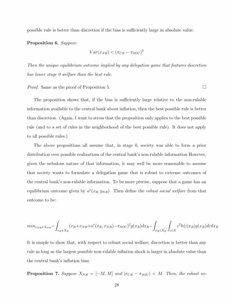
possible rule is better than discretion if the bias is su�ciently large in absolute value.

Proposition 6. Suppose:

V ar(xNR) < (⇡CB � ⇡SOC)2

Then the unique equilibrium outcome implied by any delegation game that features discretion

has lower stage 0 welfare than the best rule.

Proof. Same as the proof of Proposition 5.

The proposition shows that, if the bias is su�ciently large relative to the non-rulable

information available to the central bank about inflation, then the best possible rule is better

than discretion. (Again, I want to stress that the proposition only applies to the best possible

rule (and to a set of rules in the neighborhood of the best possible rule). It does not apply

to all possible rules.)

The above propositions all assume that, in stage 0, society was able to form a prior

distribution over possible realizations of the central bank’s non-rulable information However,

given the nebulous nature of that information, it may well be more reasonable to assume

that society wants to formulate a delegation game that is robust to extreme outcomes of

the central bank’s non-rulable information. To be more precise, suppose that a game has an

equilibrium outcome given by a

⇤(xR, yNR). Then define the robust social welfare from that

outcome to be:

minxNR2XNR�ˆxR2XR

(xR+xNR+a

⇤(xR, xNR)�⇡SOC)2g(xR)dxR�

ˆxR2XR

ˆ"2E

"

2h("|xR)g(xR)d"dxR

It is simple to show that, with respect to robust social welfare, discretion is better than any

rule as long as the largest possible non-rulable inflation shock is larger in absolute value than

the central bank’s inflation bias.

Proposition 7. Suppose XNR = [�M,M ] and |⇡CB � ⇡SOC | < M. Then, the robust so-

28

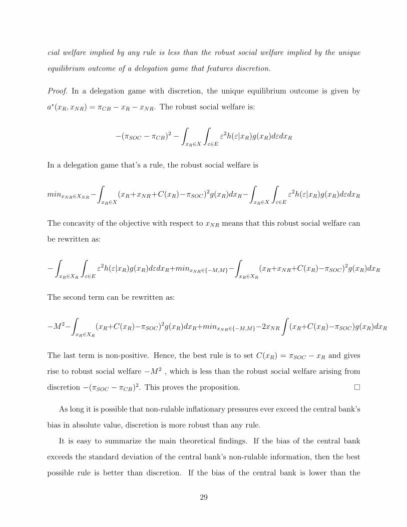
cial welfare implied by any rule is less than the robust social welfare implied by the unique

equilibrium outcome of a delegation game that features discretion.

Proof. In a delegation game with discretion, the unique equilibrium outcome is given by

a

⇤(xR, xNR) = ⇡CB � xR � xNR. The robust social welfare is:

�(⇡SOC � ⇡CB)2 �ˆxR2X

ˆ"2E

"

2h("|xR)g(xR)d"dxR

In a delegation game that’s a rule, the robust social welfare is

minxNR2XNR�ˆxR2X

(xR+xNR+C(xR)�⇡SOC)2g(xR)dxR�

ˆxR2X

ˆ"2E

"

2h("|xR)g(xR)d"dxR

The concavity of the objective with respect to xNR means that this robust social welfare can

be rewritten as:

�ˆxR2XR

ˆ"2E

"

2h("|xR)g(xR)d"dxR+minxNR2{�M,M}�

ˆxR2XR

(xR+xNR+C(xR)�⇡SOC)2g(xR)dxR

The second term can be rewritten as:

�M

2�ˆxR2XR

(xR+C(xR)�⇡SOC)2g(xR)dxR+minxNR2{�M,M}�2xNR

ˆ(xR+C(xR)�⇡SOC)g(xR)dxR

The last term is non-positive. Hence, the best rule is to set C(xR) = ⇡SOC � xR and gives

rise to robust social welfare �M

2 , which is less than the robust social welfare arising from

discretion �(⇡SOC � ⇡CB)2. This proves the proposition.

As long it is possible that non-rulable inflationary pressures ever exceed the central bank’s

bias in absolute value, discretion is more robust than any rule.

It is easy to summarize the main theoretical findings. If the bias of the central bank

exceeds the standard deviation of the central bank’s non-rulable information, then the best

possible rule is better than discretion. If the bias of the central bank is lower than the

29

standard deviation of the central bank’s non-rulable information, then all rules are worse

than discretion. Perhaps most importantly, if the largest realization of the central bank’s

rulable information exceeds its bias in absolute value, then discretion is more robust than

any rule.

5 Discussion

In this section, I discuss some aspects of the theoretical results derived above.

5.1 Inflationary Bias?

The propositions in the previous section show that rules are dominated by discretion, as

long as the central bank’s inflationary bias is small in absolute value. In this subsection, I

argue that the evidence suggests that the Federal Open Market Committee’s inflation bias

has been, at most, only modestly above zero over the past two decades.35

To make this argument, I need to first establish a benchmark for the socially optimal level

of inflation. In many countries (such as Canada and the United Kingdom), elected govern-

ments have established what are intended to be long-term targets for inflation. Presumably,

these targets can be seen as being relatively good proxies for socially optimal inflation. In the

US, no such target has been established. However, in early 2012, the Federal Open Market

Committee formally established a long-term goal of keeping PCE inflation36 at 2%. Congress

has, as yet, made no attempt to modify this target. So, I will treat the 2% target as being

equivalent to the socially desirable level of inflation (⇡SOC).

We can gauge the FOMC’s inflation bias in two di↵erent ways: in terms of the the Com-

mittee’s inflation objectives and in terms of actual outcomes. In terms of the former, in the

35The concerns about bias, both in the media and in the academe, usually focus on the possibility that theFOMC has a positive inflation bias. So, I don’t present evidence against the hypothesis that the FOMC’sinflation bias was highly negative.

36See https://www.federalreserve.gov/monetarypolicy/files/FOMC LongerRunGoals 20160126.pdf for themost recent version of this statement.

30

last meeting of each year, the Committee’s sta↵ provide inflation forecasts for the upcoming

two years. These forecasts are conditioned on the sta↵’s best projection of what the Com-

mittee will actually do. Since 1997, the one-to-two year ahead inflation forecasts have only

rarely exceeded 2% and have never been as high as 2 1/4 percent. Hence, the sta↵ did not

see the FOMC as aiming for inflation well above 2%. Since 2007, the FOMC participants

have submitted their own end-of-year inflation forecasts. As discussed earlier, these forecasts

are conditioned on each participant’s own assessment of appropriate monetary policy. The

midpoint of the central tendency of the one-to-two-year ahead PCE inflation forecasts (con-

structed by discarding the three highest and three lowest forecasts) never exceeded 2% (even

during periods of high unemployment).37

So, there is little evidence in the FOMC’s projections for inflation that the Committee

is aiming for inflation to be materially above 2%. If we look at outcomes, we get a similar

conclusion. Over the past twenty years, the sixty-month trailing average PCE inflation rate

has never been above 3%. Even here, most of the upward misses with respect to inflation

can be attributed to the surprisingly large run-up in oil prices in 2008. Over the past twenty

years, the sixty-month trailing average core PCE inflation rate (which excludes goods and

services related to food and energy) has never exceeded 2 1/4 %.

Of course, inflation rose to unacceptably high levels during the 1970s. However, since

that period, much has changed in terms of FOMC practice. Perhaps most notably, both

Chairman William Martin and Chairman Arthur Burns interacted relatively closely with the

White House compared to Chair Janet Yellen or her immediate predecessors. The Federal

Reserve is consequently much more independent of the short-term political pressures that

often are argued to have been responsible for at least part of the Great Inflation.38

37See Kocherlakota (2012).38See Meltzer (2010).

31

5.2 Communication Challenges with Rules

Over the past two decades, many central banks, including the Federal Reserve, have greatly

increased their level of communication about monetary policy. In this subsection, I briefly

argue that there is a sense in which rules (or any form of constraint on discretion) make such

communication more challenging.

In a world with discretion, the central bank sets the level of accommodation so that:

a

⇤(xR, xNR) = ⇡CB � xR � xNR

The variable xR is known to the public, but the non-rulable information xNR may or may not

be. The choice of accommodation, in and of itself, reveals (⇡CB �xNR). If the central bank’s

bias is known (as I assume above), then the choice of accommodation reveals the non-rulable

information xNR.

In contrast, if the central bank is using a rule, the choice of accommodation reveals nothing

about xNR. It may well be true, though, that the central bank would like to reveal at least

some of its private information about inflation, so as to reduce the private sector’s uncertainty

about inflation. The central bank would then need to supplement its choice of accommodation

with separate communication about xNR. In this sense, rules - or any constraints on central

bank accommodation - serve to increase the central bank’s communication challenge.

6 Conclusions

There is a broad academic macroeconomic consensus that monetary policy should be con-

strained by rules. In this paper, I argue instead that there are good reasons to believe that

societies will achieve better outcomes if central banks are given complete discretion to pur-

sue well-specified goals. Theoretically, discretion allows central banks to take advantage of

information about the macro-economy that is hard to write into rules. Empirically, deviating

32

more materially from the Taylor Rule would have allowed the FOMC to pursue a more rapid

recovery from the Great Recession.

I do show that if central banks have a su�ciently large pro-inflation bias, there exists a

set of rules that dominates discretion. (However, it is still not true that all rules dominate

discretion.) I argue in the paper that, over the past twenty years, the FOMC has shown

little if any pro-inflation bias. But this claim would be much less true in other periods in

history (like the 1970s). What changes in institutional design have served to reduce the

Federal Reserve’s inflationary bias to its current low level? I say little about this issue in the

paper, beyond referring to increased independence from the White House. However, it is a

key question for future work along these lines.

The House of Representatives has passed legislation that would require the FOMC to

treat the Taylor Rule as a key benchmark in its decision-making about policy.39 The analysis

in this paper implies that this move by the House is a mistake. It is true that the Taylor

Rule was arguably associated with good macroeconomic outcomes during a limited period

of US economic history. But so was the Riefler-Burgess framework! Enshrining the Taylor

Rule in statute can only hamstring the Federal Reserve’s response to currently unanticipated

events. The House would be much better o↵ requiring the FOMC to communicate a collective

forecast for employment and prices, and to explain clearly why policy is not being used to

close any gaps between that forecast and the Committee’s ostensible goals. That requirement

would incentivize the Committee to pursue more rapid recoveries than they did in 2009-10.

References

[1] Bernanke, B., “Monetary Policy Since the Onset of the Crisis,” speech given at the

Federal Reserve Bank of Kansas City Economic Symposium, 2012.

39Specifically, see Section 2 of H. R. 3189, the Fed Oversight Reform and Modernization Act of 2015.

33

[2] Brainard, W., “Uncertainty and the E↵ectiveness of Policy,” Papers and Proceedings

of the Seventy-ninth Annual Meeting of the American Economic Association , 1967, p.

411-426.

[3] Brunner, K., and Meltzer, A., “What Did We Learn From the Monetary Experience of

the United States in the Great Depression?” Canadian Journal of Economics 1, 1968,

p. 334-348.

[4] Canzoneri, M., “Monetary Policy Games and the Role of Private Information,” American

Economic Review 75, 1985, p. 1056-70.

[5] Eggertsson, Gauti B., and Michael Woodford, “The Zero Bound on Interest Rates and

Optimal Monetary Policy,” Brookings Papers on Economic Activity, 2003(1), p. 139-211.

[6] FOMC Bluebook, October 2009, https://www.federalreserve.gov/monetarypolicy/

files/FOMC20091104bluebook20091029.pdf.

[7] FOMC Summary of Economic Projections, November 2009, https://www.

federalreserve.gov/monetarypolicy/files/FOMC20091104SEPcompilation.pdf.

[8] FOMC transcript, December 2009, https://www.federalreserve.gov/monetarypolicy/

files/FOMC20091216meeting.pdf.

[9] FOMC transcript, March 2010, https://www.federalreserve.gov/monetarypolicy/

files/FOMC20100316meeting.pdf.

[10] FOMC transcript, October 2010, https://www.federalreserve.gov/monetarypolicy/

files/FOMC20101015confcall.pdf.

[11] FOMC Tealbook Part A, October 2010, https://www.federalreserve.gov/

monetarypolicy/files/FOMC20101103tealbooka20101027.pdf.

[12] FOMC Tealbook Part B, October 2010, https://www.federalreserve.gov/

monetarypolicy/files/FOMC20101103tealbookb20101028.pdf.

34

[13] FOMC November 2010 Summary of Economic Projections, https://www.

federalreserve.gov/monetarypolicy/files/FOMC20101103SEPcompilation.pdf.

[14] Hansen, L., and Sargent, T., Robustness, Princeton, NJ: Princeton University Press,

2007.

[15] Holmstrom, B., “On the Theory of Delegation,” in M. Boyer and R. Kihlstrom (eds.)

Bayesian Models in Economic Theory, New York: North-Holland, 1984.

[16] Kocherlakota, N., “Planning for Lifto↵,” Speech at Gogebic Community College, Iron-

wood, Michigan, 2012.

[17] Kocherlakota, N., “Rules versus Discretion: A Reconsideration,” Speech to Korea-

America Economic Association, 2015a.

[18] Kocherlakota, N. “Monetary Policy Renormalization,” Speech to Federal Reserve Bank

of Philadelphia Policy Forum, 2015b.

[19] Meltzer, A., A History of the Federal Reserve, Volume 1, 1913-51, Chicago, IL: The

University of Chicago Press.

[20] Meltzer, A., “Comment on ’Volatile Times and Persistent Conceptual Errors: U.S. Mon-

etary Policy 1914-51, by C. Calomiris’, in The Origins, History, and Future of the Federal

Reserve: A Return to Jekyll Island, ed. Michael Bordo and William Roberds, p. 219-225,

Cambridge: Cambridge University Press, 2010.

[21] Svensson, L. E. O., “Inflation Forecast Targeting: Implementing and Monitoring Infla-

tion Targets,” European Economic Review 41, p. 1111-1146, 1997.

[22] Svensson, L. E. O., and R. Tetlow, 2005, “Optimal Policy Projections,” International

Journal of Central Banking, 2005.

[23] Svensson, L. E. O., “What Is Wrong with Taylor Rules? Using Judgment in Monetary

Policy through Targeting Rules,” Journal of Economic Literature 41, 2003, p. 426-477.

35

[24] Taylor, J., “Discretion vs. Policy Rules in Practice,” Carnegie-Rochester Conf. Ser.

Public Pol. 39, 1993, p. 195–214.

[25] Wallace, Neil, “A Modigliani-Miller Theorem for Open-Market Operations,” American

Economic Review 71, 1981, p. 267-274.

[26] Walsh, C., “Optimal Contracts for Central Bankers,” American Economic Review 85,

1995, p. 150-167.

[27] Woodford, M., “Methods of Policy Accommodation at the Interest-Rate Lower Bound,”

Federal Reserve Bank of Kansas City Economic Policy Symposium, 2012.

[28] Williams, J., “A Defense of Moderation in Monetary Policy,” Federal Reserve Bank of

San Francisco working paper, 2013.

36