Root Canal Irrigation- An engineering analysis using Computational Fluid … · ·...

Root Canal Irrigation-

An engineering analysis using

Computational Fluid Dynamics

Submitted by:

Tikran Kocharian

Supervised by:

Professor Markus Bussmann

This thesis is submitted in conformity with the requirements for the degree of

Master of Engineering

Department of Mechanical and Industrial Engineering

University of Toronto

©Copyright by Tikran Kocharian

Abstract

Acknowledgments

List of Figures

1. Introduction

1.1. What is a Root Canal? …………………………………………………………………..1

1.2. Root Canal Therapy…………………….………………………………………………..1

1.3. Need for Root Canal Therapy…………………………….………………………….…..1

1.4. Root Canal Therapy Procedure…………………………………………………………..2

1.5. Risks and Complications of Root Canal Therapy………………………………………..2

1.6. Root Canal Therapy and Computational Fluid Dynamics………………………...……..2

1.7. Irrigation of the Root Canal and Irrigation Rates…………………………………....…..3

2. Literature and Theoretical Background

2.1. The Need for CFD ………………………………………………………………..……..6

2.2. The Strategy of CFD……………………………………………………………………..7

2.3. Discretization Using The Finite-Volume Method……………………………………….8

2.4. ICEM CFD as a CFD Tool………………………………………….…….………….…10

2.5. FLUENT as a CFD Tool……………………………………………………...………...10

2.6. Steps in Solving a CFD Problem………………………………………………….……11

(i)

3. Methodology

3.1. Geometry Reconstruction…………………………………………………...………….12

3.2. Computational Mesh Generation………………………………………….……………13

3.3. Boundary and Operating Conditions……………………………………………..…….14

3.4. Flow Assumptions……………………………………………………………….……..15

3.5. Naming conventions for simulations setups…………………………….……………...16

3.6. Solver Setup……………………………………………………………….……………16

4. Results and Discussion

4.1. Wall Shear Stress(WSS)…………………………………………………………...…...19

4.2. In-Plane Velocity vectors at the irrigation needle vent………………………….……...19

4.3. Velocity by Velocity magnitude contours at cross sections…………………….……....20

4.4. Simulations Results Summary Table…………………………………………………...21

5. Conclusion........................................................................................................22

6. Future Discussions...........................................................................................22

References.........................................................................................................54

(ii)

Abstract

Aim:

Despite more than a century of technological improvements in root canal procedures, clinical

studies indicate that bacteria remain in the canal following standardized cleaning and shaping

procedures using irrigants.

The most common method of evaluating root canal bacteria assesses growth from paper point

samples [1], in effect measuring what is removed from the root canal rather than what remains

behind. Many studies have attempted to determine the efficacy of chemical and mechanical

debridement during endodontic therapy [2].

In the present study, computational fluid dynamics is utilized to study the velocity distribution

of irrigant flow in the root canal, wall flow pressure, and wall shear stress on the root-canal wall,

which are difficult to measure in vivo because of the microscopic size of the root canals.

Methodology:

Computational Fluid Dynamics was used to evaluate and predict regions of fast and slow flow

formation and the overall effectiveness of irrigation during non-surgical root canal therapy.

Simulations were set using ICEM CFD 12.1 for meshing and FLUENT 12.1.4.The flow analyses

were conducted for two real-life clinical mass flow rates of irrigants (0.15 and 0.30 mL/sec) and

two conditions of irrigation needle inside the root canal (3 mm and 2 mm short of the bottom of

the root canal).

(iii)

Results: Contours of the Dynamic pressure and Wall shear stress (WSS) along the root canal

and velocity magnitude with velocity vectors at different cross section locations were obtained

and discussed.

Conclusion : Changes in irrigant flow rate and the irrigant needle insertion inside the root canal

influence flow velocity, wall shear stress and the dynamic pressure.

In addition, existence of weak wall shear stress values in the apical third of the root canal was

confirmed.

Computational Fluid Dynamics could be a valuable tool in assessing the further implications of

additional model considerations on all important parameters for the effectiveness and safety of

root canal therapy.

(iv)

Acknowledgments

I gratefully acknowledge the contribution of the following people for their moral

support and for the help that was instrumental bringing this report to fruition.

I am grateful to Prof. Pierre Sullivan for trusting and granting me a chance to study and earn my

graduate degree at the University of Toronto.

My sincere gratitude to Prof. Markus Bussmann for his support, continuous supervision and

guidance during my studies at University of Toronto.

I would like to express my appreciations to Ms. Jho Nazal; graduate program assistant from th e

Graduate office of Mechanical and Industrial Engineering for her continuous help and moral

support all the way through the program.

I am thankful to Mr. Babak Emami for his support and advice during the project and the process

of simulations and data collection.

I acknowledge the clinical support assistance and consultation provided to me by Dr. Anil

Kishen and Dr. Babak Nurbakhsh from the faculty of Dentistry, University of Toronto.

Finally, My soul mate and best friend Catherine, for her everlasting inspiration and

sacrifices she has made for over a decade and during my studies. It would not have been

possible to make it this far without her love, kindness and wisdom.

(v)

List of Figures

Figure 1- Filing and Irrigation Processes during a typical Root Canal Treatment ……………..25

Figure 2- Clinical examples of severe Canal Curvatures in roots ………………………………26

Figure 3- Flowchart of steps to be followed for solving a typical CFD problem ………………27

Figure 4- Geometrical characteristics of the root canal model used in the present study ……...28

Figure 5- Geometrical characteristics and setup of the root canal for two sets of …………......28

Irrigation needle insertion .

Figure 6- Dynamic pressure contour along the root canal for RFRD setup ……………………29

Figure 7- Velocity magnitude contour along the root canal for RFRD setup …………………..30

Figure 8- Detail of the velocity vectors by velocity magnitude at the needle ………………….31

vent for RFRD setup.

Figure 9- Dynamic pressure contour along the root canal for DFRD setup ……………………32

Figure 10- Velocity magnitude contour along the root canal for DFRD setup …………………33

Figure 11- Detail of the velocity vectors by velocity magnitude at the needle …………………34

vent for DFRD setup.

Figure 12- Dynamic pressure contour along the root canal for RFINSD setup ………………..35

Figure 13- Velocity magnitude contour along the root canal for RFINSD setup ………………36

Figure 14- Detail of the velocity vectors by velocity magnitude at the needle ………………...37

vent for RFINSD setup.

Figure 15- Dynamic pressure contour along the root canal for DFINSD setup ………………..38

(vi)

Figure 16- Velocity magnitude contour along the root canal for DFINSD setup ………………39

Figure 17- Detail of the velocity vectors by velocity magnitude at the needle …………...........40

vent for DFINSD setup.

Figure 18- Distribution of the Wall Shear Stress for RFRD setup ……………………………...41

Figure 19- Distribution of the Wall Shear Stress for DFRD setup …………………………….42

Figure 20- Distribution of the Wall Shear Stress for RFINSD setup ………………………….43

Figure 21- Distribution of the Wall Shear Stress for DFINSD setup ………………………….44

Figure 22- Contours of velocity vectors at the irrigant needle vent for RFRD setup …………45

Figure 23- Contours of velocity vectors at the irrigant needle vent for DFRD setup…………46

Figure 24- Contours of velocity vectors at the irrigant needle vent for RFINSD setup………..47

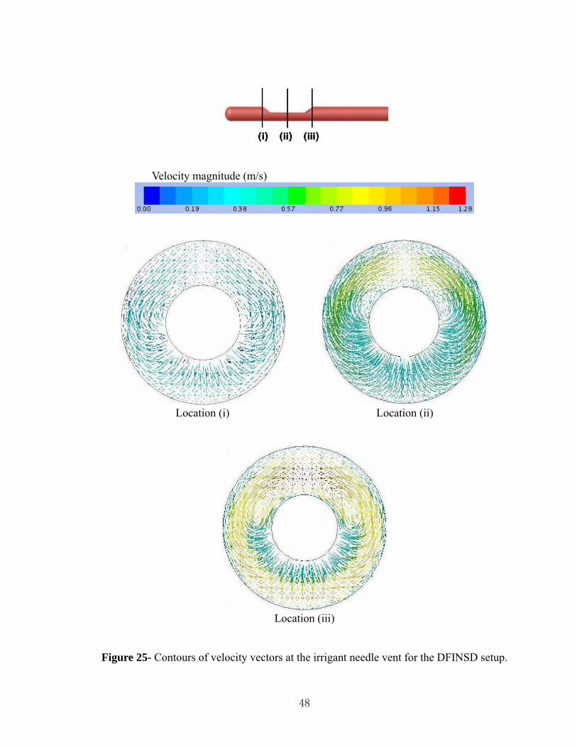
Figure 25- Contours of velocity vectors at the irrigant needle vent for DFINSD setup………..48

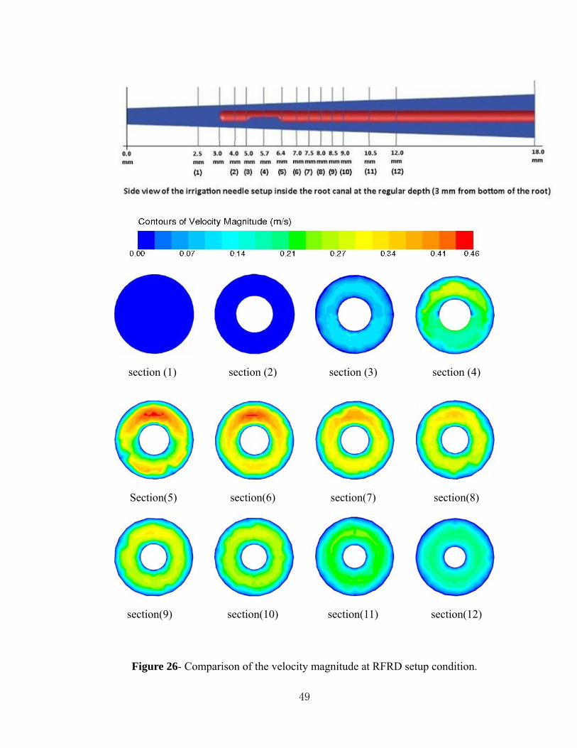
Figure 26- Comparison of the velocity magnitude at RFRD setup condition ………………….49

Figure 27- Comparison of the velocity magnitude at DFRD setup condition ………………….50

Figure 28- Comparison of the velocity magnitude at RFINSD setup condition ……………….51

Figure 29- Comparison of the velocity magnitude at DFINSD setup condition ……………….52

Figure 30- Comparison of the velocity magnitude at the exit of the side vent …………………53

at 4 setup conditions.

(vii)

1. Introduction

1.1. What is a Root Canal?

Underneath tooth's outer enamel and within the dentin is an area of soft tissue called

the pulp tissue. While a tooth's pulp tissue does contain nerve fibers, it is also composed of

arteries, veins, lymph vessels, and connective tissue. Each tooth's nerve enters the tooth at the

very tip of its roots. From there, the nerve runs through the center of the root in small "root

canals," which join up with the tooth's pulp chamber. Root canals are very small, thin divisions

that branch off from the top pulp chamber down to the tip of the root. A tooth has at least one but

no more than four root canals [3].

1.2. Root Canal Therapy

Root canal treatment is a “non-surgical” approach used to treat two distinct

endodontic disease entities: (1) “extirpated” vital, but irreversibly inflamed pulp-the soft tissue

inside the tooth that contains nerves, blood vessels, and connective tissue, where the goal is to

maintain existing health around root canal apex (periapical) and thus prevent periapical disease;

or (2) the non-vital or dying, infected pulp, associated with apical periodontitis.

1.3. Need for Root Canal Therapy

Root canal therapy is necessary because the tooth will not heal by itself. Without

treatment, the infection will spread, bone around the tooth will begin to degenerate and the tooth

may fall out. Pain usually worsens until one is forced to seek emergency dental attention.

The only alternative is usually extraction of the tooth, which can cause surrounding teeth to shift

crookedly, resulting in a bad bite.

1

1.4. Root Canal Therapy Procedure

Root Canal Therapy is a procedure done to remove the damaged or dead pulp in the

root canal of the tooth by cleaning out the diseased pulp and reshaping the canal. The canal is

filled with a rubberlike substance called gutta–percha or another material to prevent

recontamination of the tooth (Figure 1). The tooth is then permanently sealed, with possibly a

post and/or a crown made of porcelain or metal alloy. This enables patients to keep the original

tooth.

1.5. Risks and complications of Root Canal Therapy

More than 95 percent of root canal treatments are successful. However, sometimes a

procedure needs to be redone due to diseased canal offshoots that went unnoticed or the fracture

of a filing instrument, both of which rarely occur. Occasionally, a root canal therapy will fail

altogether, marked by a return of pain.

Managing severe Canal Curvatures in roots (Figure 2) , is another challenge in performing a

successful root canal therapy [4]

1.6. Root Canal Therapy and Computational Fluid Dynamics

The hydrodynamics of the root canal are different than in macro environments.

Computational fluid dynamics is an area of research usually associated with large-scale

phenomena and related problems but fluid flow problems exist at the microscopic level of the

root canal systems as well.

Computational fluid dynamics (CFD) represents a powerful tool to investigate flow

patterns and physical and chemical phenomena by mathematical modeling and computer

2

simulation. CFD simulations can provide details on the velocity field in areas where

experimental measurements are difficult to perform. Furthermore, important properties such as

shear stress and pressure can easily be obtained, in contrast to experiments, especially in micro-

scale flow problems. Recently, a CFD model was implemented for the evaluation of irrigant flow

in the root canal [5].

CFD technology enables a complex numeric simulation of root canal irrigation;

permits the simulation of real physical conditions, and the determination of associated complex

parameters.

This study utilizes computational fluid dynamics to evaluate and predict specific

parameters, such as the streamline, velocity distribution of irrigant flow in the root canal, wall

flow pressure, and wall shear stress (WSS) on the root-canal wall, which are difficult to measure

in vivo because of the microscopic size of the root canals.

1.7. Irrigation of the Root Canal and Irrigation rates

Instrumentation has long been considered the cornerstone of endodontic treatment,

yet the addition of irrigant will further improve the bacterial elimination. The results of an

earlier study showed that there is a significant reduction in bacteria after irrigation with

antimicrobial solution [6].

During and after instrumentation; some organic tissues and bacteria are often left

inside root canal systems, because of the anatomic complexity of the pulp space. The irrigants

facilitate removal of such microorganisms, tissue remnants, and dentin chips from the root canal

through a flushing mechanism .

3

Irrigants can also help prevent packing of the hard and soft tissue in the apical root

canal and extrusion of infected material into the periapical area [7].

In addition to antimicrobial effects and tissue dissolution, microorganisms and debris are flushed

out of the root canal by the washing action of the irrigant [8].

Irrigants must be brought into direct contact with the entire canal area and especially

with the apical portions of narrow root canals for optimal effectiveness. As previous studies have

shown, penetration and flushing action of the irrigant depend on the anatomy of the root canal

system and the system of delivery, the volume and fluid properties of the irrigant, and the size,

type, and insertion depth of the irrigation needle[8].

Irrigation dynamics should be considered when evaluating the effect of an irrigant

on root canal contents. The penetration of the irrigant and the flushing action created by

irrigation are dependent not only on the anatomy of the root canal system such as size of

enlarged root canal (radius of tube), but also on the system of delivery, the depth of

placement(insertion), and the volume and fluid properties of the irrigant.

Other factors influencing efficacy of irrigation include velocity of the irrigating

solution at the tip of the needle and the orientation of the bevel of the needle.

Irrigant velocity on root canal wall is one of the most significant fluid mechanics parameters. It

allows the evaluation of the velocity loss of the irrigant through the canal as well as the velocity

imparted by the moving irrigant.

In brief, irrigant velocity and dynamics in the wall region play a significant role in

debris deposition, tissue dissolution, and antimicrobial effectiveness.

4

Higher initial velocities might result in increased possibilities of irrigant or air extrusion towards

the periapical bone area, with considerable implications for the patient, such as discomfort and

possible swelling.

There is a delicate balance when it comes to irrigation during the root canal therapy.

Under-irrigation can leave traces of bacteria, while over-irrigation can cause tissue damage and

even pain.

Previous study has showed that instrumentation beyond a size 35 may allow penetration of

irrigant beyond the apex into periapical tissues [2].

5

2. Literature and Theoretical Background

2.1. The Need for CFD

Applying the fundamental laws of mechanics to a fluid gives the governing

equations for a fluid. The conservation of mass equation is

and the conservation of momentum equation is

These equations along with the conservation of energy equation form a set of

coupled, non- linear partial differential equations. It is not possible to solve these equations

analytically for most engineering problems [9].

However, it is possible to obtain approximate computer-based solutions to the governing

equations for a variety of engineering problems. This is the subject matter of Computational

Fluid Dynamics (CFD).

In CFD modeling, a complex geometry is separated into a large number of smaller

finite elements, creating a grid on which the equations describing the phenomenon are

discretised. By assuming the velocity field within them, it is possible to solve the equations of

motion at the nodes connecting these elements, provided that certain boundary conditions for

velocity and pressure are imposed. From this solution arise the measurements of wall shear

stress and other parameters.

6

The advantage of CFD compared to the other in vitro and in vivo techniques, as well

as to simple theoretical models based on poiseuille flow, is that it provides invaluable

knowledge of the detailed variations related to time and space that shear stress may exhibit,

while the parameters that determine each set of conditions are completely controlled.

2.2. The Strategy of CFD

The strategy of CFD is to replace the continuous problem domain with a discrete

domain using a grid. In the continuous domain, each flow variable is determined at every point

in the domain. For instance, the pressure p in the continuous 1-D domain shown in the figure

below would be given as

( )p p x , 0 1x (3)

In the discrete domain, each flow variable is defined only at the grid points. Hence, in the

discrete domain shown below, the pressure could be determined only at the N grid points.

( )i ip p x , 1, 2,...,i N

Continuous Domain Discrete Domain

0 1x 1 2, ,..., nx x x x

0x 1x 1x ix nx

(grid point) Coupled partial differential equations - Coupled algebraic equations in Boundary Conditions in continuous variables discrete variables

In a computational fluid dynamics solution, one would directly solve for the relevant

flow variables only at the grid points. The values at other locations are determined by

interpolating the values at the grid points.

The governing partial differential equations and boundary conditions are described in terms of

7

the continuous variables pressure and velocity vector etc. One can approximate these in the

discrete domain in terms of the discrete variables ip ,etc.

The discrete system is a large set of coupled, algebraic equations in the discrete variables.

Setting up the discrete system and solving it (as a matrix inversion problem) involves a large

number of repetitive calculations, a task humans leave it to the digital computer.

FLUENT code uses the Finite-Volume method. When it is used, the code directly solves for

values of the flow variables at the cell centers; values at other locations are obtained by suitable

interpolation.

2.3. Discretization Using the Finite-Volume Method

In the finite-volume method, quadrilaterals are commonly referred to as a “cell” and

a grid point as a “node”. In 2-D, one could also have triangular cells. In 3-D, cells are usually

hexahedral, tetrahedral (present study case), or prism. In this approach, the integral form of the

conservation equations is applied to the control volume defined by a cell to get the discrete

equations for the cell. The integral form of the continuity equation for steady, incompressible

flow is

The integration is over the surface S of the control volume and n is the outward

normal at the surface. Physically, this equation means that the net volume flow into the control

volume is zero. Consider the rectangular cell shown below.

8

The velocity at face i is taken to be

Applying the mass conservation equation (4) to the control volume defined by the cell gives:

1 2 3 4 0u y v x u y v x (5)

This is the discrete form of the continuity equation for the cell. It is equivalent to

summing up the net mass flow into the control volume and setting it to zero. So it ensures that

the net mass flow into the cell is zero i.e. that mass is conserved for the cell. Usually, but not

always, the values at the cell centers are solved for directly by inverting the discrete system.

The face values , etc. are obtained by suitably interpolating the cell-center

values at adjacent cells. Similarly, one can obtain discrete equations for the conservation of

momentum and energy for the cell.

1 2,u v

One can readily extend these ideas to any general cell shape in 2-D or 3-D and any

conservation equation. When using FLUENT, it’s useful to remember that the code is finding a

solution such that mass, momentum, energy and other relevant quantities are being conserved

for each cell.

9

Also, the code directly solves for values of the flow variables at the cell centers;

values at other locations are obtained by suitable interpolation.

2.4. ICEM CFD as a CFD tool

From Computer Aided Design to mesh generation for analysis, ANSYS ICEM CFD

provides sophisticated geometry acquisition, mesh generation, post-processing and mesh

optimization tools. It is the only universal pre- and post-processor for computational fluid

dynamics analysis and other computer aided engineering applications.

ANSYS ICEM CFD’s mesh generation tools offer the capability to parametrically

create grids from geometry in multi-block structured, unstructured hexahedral, tetrahedral,

hybrid grids consisting of hexahedral, tetrahedral, pyramidal and prismatic cells; and Cartesian

grid formats combined with boundary conditions [10] .

2.5. FLUENT as a CFD tool

ANSYS FLUENT is a computer program written in the C computer language for

modeling fluid flow in simple and complex geometries. It provides complete mesh flexibility,

including the ability to solve flow problems using unstructured meshes that can be generated

about complex geometries with relative ease [11].

FLUENT, a finite volume solver is used to solve the discrete Navier-Stokes equations. The

computational method allows researchers to get results quickly (depending on the complexity)

and visually close to reality.

10

After a mesh has been read into ANSYS FLUENT, all remaining operations are

performed within ANSYS FLUENT. These operations include setting boundary conditions,

defining fluid properties, executing the solution, refining the mesh, and post processing and

viewing the results.

2.6. Steps in Solving a CFD Problem

Once the important features of the problem have been determined, the basic procedural steps

should be followed (Figure 3).

1. Modeling goals must be defined.

What results are you looking for, and how will they be used?

What simplifying assumptions one has to make?

What simplifying assumptions can be made?

2. Model geometry and mesh must be created.

ANSYS FLUENT 12.1.4 uses unstructured 3-D meshes in order to reduce the amount of time

spent generating meshes, to simplify the geometry modeling and mesh generation process, to

allow modeling of more complex geometries than one can handle with conventional, multiblock

structured meshes, and to let one adapt the mesh to resolve the flow field features.

3. Solver and physical models set up.

4. Compute and monitor the solution.

5. Examine and save the results.

6. Consider revisions to the numerical or physical model parameters, if necessary.

11

3. Methodology 3.1. Geometry Reconstruction

A CFD model was created to simulate the irrigant flow inside a prepared root canal

and to investigate the effect of irrigation needle depth and mass flow rate on flow patterns by

using a three dimensional computational fluid dynamics model.

The root canal was simulated as a geometrical frustum of a cone (the portion of a

cone which lies between two parallel planes cutting the solid). The apical constriction and apical

foramen were not simulated because they were not within the focus of this study. The apical

terminus of the root canal was simulated as an impermeable wall.

The length of the root canal model was 18 mm; the diameter was 1.57 mm at the

canal orifice and 0.45 mm (ISO size 45) at the most apical point (6.2% taper). This shape is

consistent with the root canal model used in the experimental setup [13], and is the result of

mechanical preparation (drilling and filing).

A 30-gauge KerrHawe (KerrHawe SA, Bioggio, Switzerland) side-vented needle

with a safety tip was employed [5].

Despite the findings of many studies that recommend canal preparation with files

larger than 30/35 gauge for better penetration of irrigants and elimination of bacteria during

cleaning and shaping, a more recent study has found that apical instrumentation to a 30 size file

with 0.06 coronal taper is effective for the removal of debris and smear layer from the apical

portion of root canals [12].

12

The external and internal diameter and the length of the irrigant needle were defined

as 320extD m , int 196D m and l = 31 mm, respectively.

The needle was centered within the canal and immovable, 3 mm short of the working length

(Figure 4). This setup allows for the evaluation of irrigant flow apically to the needle tip, the

most challenging area for irrigation. An additional case was modeled to study the effect of 1 mm

further insertion of the needle (2 mm short of the working length) inside the root canal (Fig. 5).

In both cases, the needle remained parallel to the longitudinal axis of the root canal

3.2. Computational Mesh Generation

The preprocessor ICEM CFD 12.1 was used to build the 3-dimensional geometry.

The inlet, outlet, and wall surface of the flow domain were also defined in the ICEM CFD 12.1

software. 668454 unstructured tetrahedral 3-D meshes were constructed. The fluid flowed into

the simulated domain through the needle inlet (vent) and out of the domain through the root

canal orifice where atmospheric pressure was imposed.

The root canal and needle were assumed to be completely filled with the irrigant.

Gravity was included in the flow field in the direction of the negative z axis.

The commercial CFD code FLUENT 12.1.4 (Fluent Inc) was used to set up and

solve the problem. Detailed settings of the solver can be found in another study [13].

Computations were performed in a computer cluster (AMD processors) running 64-

bit SUSE Linux 10.1. The flow field for four types of setup were calculated and compared in

terms of velocity, shear stress, and apical pressure.

13

3.3. Boundary and Operating Conditions

In an internal domain, flow is considered laminar or turbulent based on the Reynolds

number (Re), a non-dimensional quantity calculated according the formula:

ReVD

(6)

where ρ is the fluid density, V is the average fluid velocity, D is the domain diameter, and μ is

the fluid viscosity.

Calculations were carried out for two selected flow rates of 0.15 mL/sec and 0.30 mL/sec, as a

common velocity and duration for irrigation in clinical practice.

In the present study Re varied between 1152–2441 for the two cases and was

calculated at the needle inlet (Table 1).Average fluid velocity (V) was calculated from irrigant

volume flow & D was calculated at the needle vent. No turbulence mode was used, as the flow

under these conditions inside the needle lumen) was expected to be laminar.

In a similar study, no turbulence was observed in both CFD and high-speed imaging

studies using similar setups [14]. The formation of vortices and unsteady flow should not

mistakenly be interpreted as turbulence (Figures 22-25). Even though the irrigant in the most

apical part of the canal may be rotating inside a vortex, this does not ensure complete

14

replacement of irrigant flow inside the root canal.

Reynolds number (Re) in the rest of the domain is probably lower, owing to the fact

that as the flow area increases, the velocity has to decrease, due to mass conservation.

Calculated values are considered low or moderate and characterize the flow as laminar or

transitional (in the critical zone).

3.4. Flow Assumptions

No-slip boundary conditions were applied to the walls of the root canal and that of

the needle, under the hypothesis of rigid, smooth and impermeable walls. Wall roughness is

expected to have a limited effect on pressure drop as long as the flow remains laminar [15], but

it may induce vorticity or even turbulence in the flow [16].

The fluid flowed into the simulated domain through the needle inlet and out of the

domain through the root canal orifice, where atmospheric pressure was imposed.

The canal and the needle were assumed to be completely filled with irrigant.

A velocity inlet boundary condition was selected for the inlet of the needle.

The irrigant was distilled water, and it was modeled as an incompressible and

homogenous Newtonian fluid with a density ρ = 998.2 kg/m3 and a constant viscosity μ=

1.0x kg/m-s. 310

Gravity was included in the flow field in the direction of the negative Z-axis.

Recently there have been a number of CFD studies in this field using such flow assumptions [8,

13, 14 and 17].

15

3.5. Naming conventions for simulations setups

In order to maintain an easier access to the simulation results and efficient data management, the

following conventions were used for naming the four different setups.

RFRD(Regular Flow, Regular Depth)-Case of a regular flow (0.15ml/sec) of irrigant and a

setup of the irrigant needle 3mm from working length (bottom of the root canal).

DFRD(Double Flow, Regular Depth)-Case of an increased flow (0.30ml/sec) of irrigant and a


RFINSD(Regular Flow, Inserted Depth)-Case of a regular flow (0.15ml/sec) of irrigant and a


DFINSD(Double Flow, Inserted Depth)-Case of an increased flow (0.30ml/sec) of irrigant and

a setup of the irrigant needle 2mm from working length (bottom of the root canal).

3.6. Solver Setup

The following steps were taken guidelines to ensure the CFD simulations and calculations using

FLUENT 12.1.4 were a success.

Pressure, velocity, wall flux shear stress and vorticity in selected areas of the flow

domain were also monitored to ensure adequate convergence in every time-step.

16

In order to avoid any unstable or divergent behavior, the under-relaxation factors for

energy, was reduced to about 0.1.

Node-based gradients with unstructured tetrahedral meshes were used.

Residuals history was used to monitor convergence and residual plots can show

when the residual values have reached the specified tolerance.

“Mesh Check” was performed to check the quality of mesh and to avoid problems

due to incorrect mesh connectivity and other potential problems.

Maximum cell skewness was checked to be below 0.98 and it was 0.59998.

17

4. Results and Discussion

Results of the simulations are presented as distribution charts of the Wall shear stress (WSS) and

contours of the velocity magnitude with velocity vectors at specific regions of interest along the

root canal simulated geometry.

The significance of the axial z-velocity magnitude for irrigant replacement has been discussed

previously [5]. Irrigant velocity on root canal wall is one of the most significant fluid mechanics

parameters. It allows the evaluation of the velocity loss of the irrigant through the canal as well

as the velocity imparted by the moving irrigant [8].

In this study, irrigant flow inside a root canal was evaluated by a modified model of a previously

published CFD simulation [13].

Various representative planes along the root canal working length were considered and the major

flow variables such as velocity and WSS were plotted as a function of distance (grid densities).

The velocity profiles were extracted from twelve cross-sectional locations along the root canal.

First case was set at 3mm from working length (irrigating needle from bottom of the root canal)

with 12 cross sections at 2.5mm,4.0mm,5.0mm,5.7mm,6.4mm,7.0mm,7.5mm,8.0mm

8.5mm,9.0 mm,10.5mm and 12.0 mm from bottom of the root canal.

18

Second case was set at 2mm from working length where irrigating needle was inserted one

millimeter deep inside the root and closer to the bottom of the canal. The 12 cross sections were

1.5mm,3.0mm,4.0mm,4.7mm,5.4mm,6.0mm,6.5mm,7.0mm,7.5mm,8.0 mm,9.5mm and 11.0

mm from bottom of the root canal).

4.1. Wall Shear Stress(WSS)

Wall Shear tress(WSS) is the force acting tangential to the surface due to friction. Its unit

quantity is pressure .The importance of this characteristic is in the tangential nature, as it has a

direct impact in the quality and efficacy of the root canal wall debridement.

Figures 18 to 21 represent the results of the wall shear stress along the longitudinal plane in the

root canal. As the wall shear stress is increased from bottom of the root canal (zero working

length) towards the exit orifice(full working length),it reaches the maximum around the irrigant

needle vent area .

It also appears that wall shear stress values are considerably low from zero working length up to

the irrigation needle vent where it drastically increases. This can result in a poor and inefficient

debridement in the apical third due to the lack of tangential force acting on the inner surface of

the root canal .This area, known as “Dead Zone” as well, has always been a challenge for

endodontists.

4.2. In-Plane Velocity vectors at the irrigation needle vent

Figures 22 to 25 present the in-plane velocity vectors at three cross sections of irrigant needle

vent (i to iii).

19

The irrigant followed a circular path at the exit of the irrigation needle vent (Location (ii) in

Figures 22 to 25).Such paths grew with an increase in irrigant flow, as well as the insertion

depth of the irrigant needle.

A series of three counter-rotating vortices were identified at the irrigation needle vent as flow

entered the root canal.(Figures 22 to 25).

The irrigation fluid established such vortices at location (iii) of all four conditions (the upper

edge of the needle vent). Vortices grew with an increase in needle insertion depth (comparison of

location (iii) in Figures 24 and 25). By comparing the location (iii) in Figures 22 and 23, in case

of an increase in the irrigant flow, same nature of increase in vortices was observed.

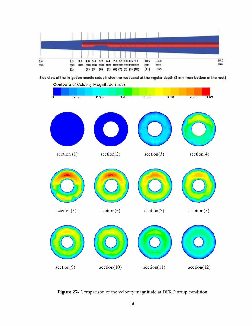
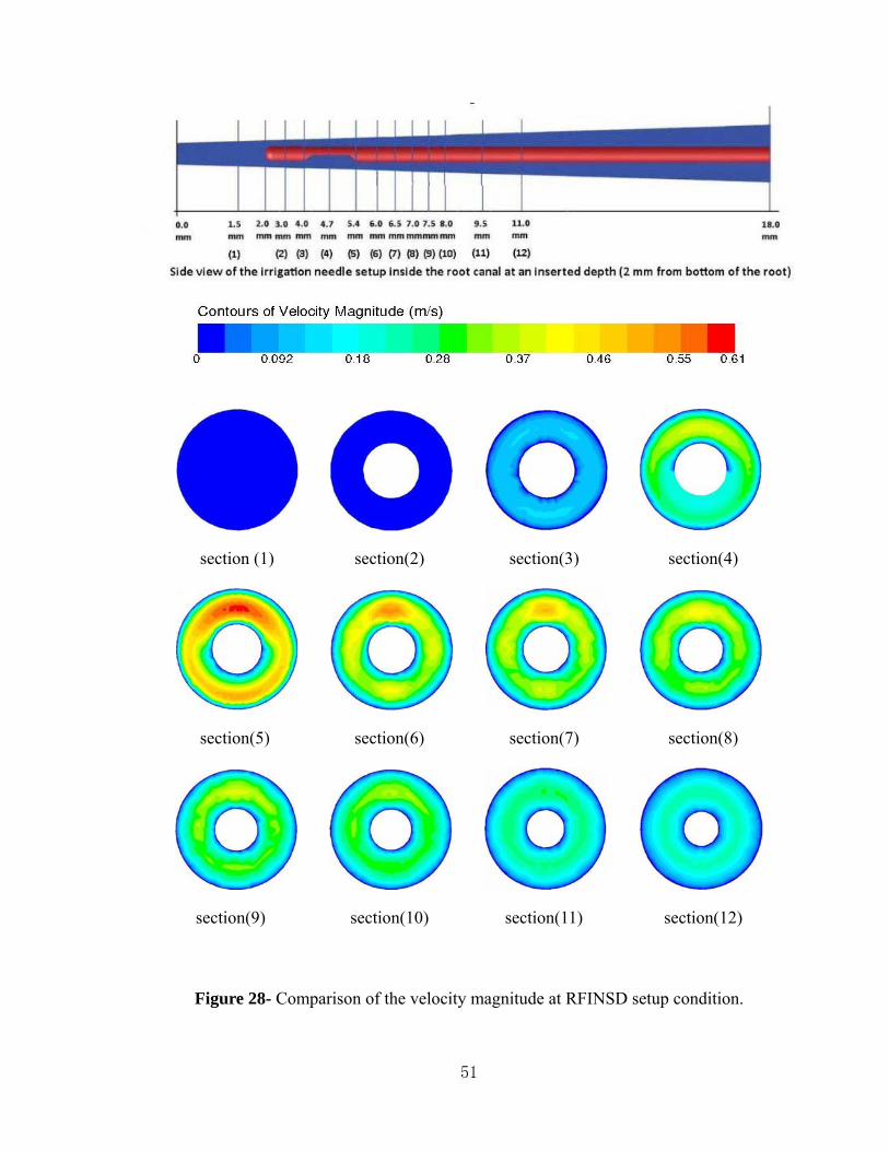
4.3. Velocity by Velocity magnitude contours at cross sections

Figure 26 to 29 present the in-plane velocity contour at cross sections selected along the root

canal working length for four setup conditions.

Results for sections (1) and (2) in figures 26 to 29 suggest a velocity of zero in plane. In other

words, there is no or negligible velocity or flow movement under the irrigant needle tip. This is

the area of the challenging apical third in the root canal, known as “Dead Zone” as well.

Figures 8,11,14 and 17 confirm the fact of a very weak flow movement towards the space

between bottom of the root canal and the irrigant needle.

Figure 30 presents the comparison of the in-plane velocity by velocity magnitudes at the exit of

the side vent at four setup conditions (RFRD-DFRD-RFINSD-DFINSD).

20

The velocity magnitude at the cross section for the simulation of all cases looks appeared to

have a similar pattern.

4.4. Simulations Results Summary Table The following table represents a summary of the important characters that were observed during

the different simulation setups.

Irrigant flow

(mL/sec)

Dynamic Pressure

(Pa)

Wall Shear Stress

(Pa)

Max. Velocity Magnitude

(m/s)

(i) RFRD 0.15 104.30 17 0.48 (ii) DFRD 0.30 424.28 45 0.92 (iii) RFINSD 0.15 188.44 26 0.61 (iv) DFINSD 0.30 786.07 70 1.30

Table 2.Simulations result summary

As it appears from the last column of the table, an increase of twice the irrigant flow (from

(RFRD to DFRD), resulted in increasing the maximum velocity to double the original

magnitude for the irrigant.

Results of changing the irrigant flow from RFINSD to DFINSD was in agreement with the

previous flow rate alteration. As the flow increased to twice the original size, the magnitude of

the maximum velocity doubled.

Changes for wall shear stress and Dynamic pressure followed the same pattern, as the irrigant

flow was increased.

21

5. Conclusion In conclusion, the results suggested that irrigant flow rate and depth of the irrigation needle

insertion does not alter the flow pattern.

The change in irrigant flow rate and the irrigant needle insertion inside the root canal influence

flow velocity, wall shear stress and the dynamic pressure.

Computational Fluid Dynamics could be a valuable tool in assessing the further implications of

needle tip design, two-phase flow (air-irrigant) and two-state (solid-fluid) model considerations

on all important parameters for the effectiveness and safety of irrigation.

The weakness of Wall shear stress values from zero working length (bottom of the root canal)

up to the irrigation needle vent confirms the fact that debridement in the apical third has always

been a challenge, this area was the focus of this study.

22

6. Future Directions

The unique nature of this project was due to the collaboration between two major branches of

science, Engineering and Dentistry. Provided time and budget, future attempts could be made to

enhance this study and proceed with further improvements of non-surgical Root Canal Therapy.

It can be achieved by considering more complex conditions and ‘real-life’ clinical challenges as

an input, directly from dentists and endodontists. Such future attempts may include but not

limited to:

Using an irrigation solution which preferably will have disinfectant, organic

debris dissolving and chelating properties which has been previously suggested[18].

Utilizing a three-dimensional Computer-Aided analyzing system in root canal

therapy to evaluate the root canal geometry before and after preparation and quantitatively

analyze the changes and movement. This can be achieved by measuring changes in root canal

diameter profile area, ‘thickness’(diameter), and root canal bending angle, the movements of

root canal geometry of the centerline before and after the root canal preparation.

Future studies with 3-D models based on real root canals of different shapes and

high resolution micro–computed tomography scans are needed to better understand the effect of

canal wall surface texture to fluid flow [19].

23

Study of the Root Canal Therapy as an interaction of fluid (irrigant) with

deformable solids (tissue) while cleaning the canal from debris [20].This can have a large impact

on the improvement of debridement and irrigation efficiency in root canal therapy process.

Study of the Root Canal Therapy as a “two-phase” flow. This involves the liquid,

a 1% solution of sodium hypochlorite or distilled water as liquid irrigant. The gaseous phase will

be air to be considered as an incompressible, Newtonian fluid. In this type of multiphase flow,

the density of the two phases can differ by a factor of about 1000.

Study of the various needle designs and their effects in the present CFD study.

This includes using open-ended vs. close-ended, notched needle group. The results of previous

studies has showed that needle tip design influences flow pattern, flow velocity, and apical wall

pressure, all important parameters for the effectiveness and safety of irrigation.

The CFD could be a valuable tool in assessing the implications of needle tip design on these

parameters [8 and 14]. Other commercially available 30-G needles which can be used in further

simulations of clinical practices include: Open-ended needles with flat, beveled and notched

styles and close-ended needles with side-vented, double side-vented and multi-vented styles.

Study the effect of off-centre positioning of the needle on the velocity magnitude

in the sectional planes as calculated by the CFD model for the cases with regular and increased

irrigant flows.

24

a) Filing

b) Irrigation

Figure 1- Filing and Irrigation Processes during a typical Root Canal Treatment (Courtesy of James L. Menius, DDS, PA web page)

25

Figure 2- Clinical examples of severe Canal Curvatures in roots.

26

Figure 3- Flowchart of steps to be followed for solving a typical CFD problem.

27

Figure 4- Geometrical characteristics of the root canal model used in the present study

Figure 5- Geometrical characteristics and setup of the root canal for two sets of irrigation

needle insertion .

28

Figure 6- Dynamic pressure contour along the root canal for RFRD setup.

(Longitudinal plane and the needle vent are shown.)

29

Figure 7- Velocity magnitude contour along the root canal for RFRD setup.


30

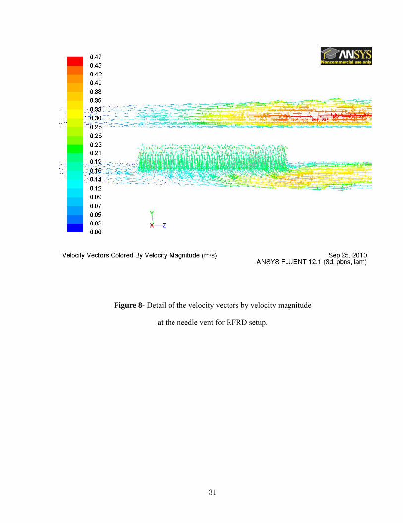
Figure 8- Detail of the velocity vectors by velocity magnitude

at the needle vent for RFRD setup.

31

Figure 9- Dynamic pressure contour along the root canal for DFRD setup.


32

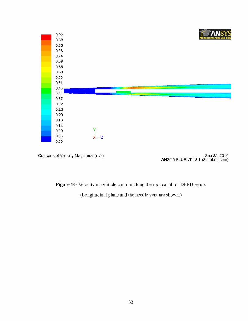
Figure 10- Velocity magnitude contour along the root canal for DFRD setup.


33


at the needle vent for DFRD setup.

34

Figure 12- Dynamic pressure contour along the root canal for RFINSD setup.


35

Figure 13- Velocity magnitude contour along the root canal for RFINSD setup.


36


at the needle vent for RFINSD setup.

37

Figure 15- Dynamic pressure contour along the root canal for DFINSD setup.


38

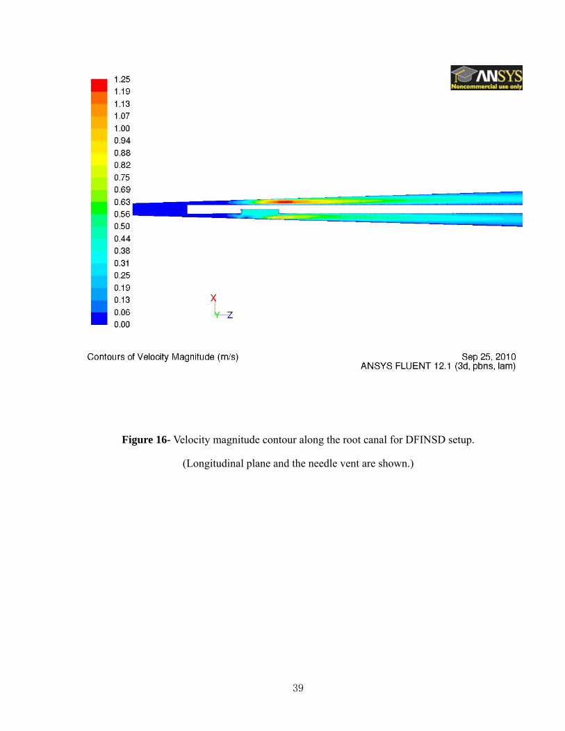
Figure 16- Velocity magnitude contour along the root canal for DFINSD setup.


39


at the needle vent for DFINSD setup.

40

Figure 18- Distribution of the Wall Shear Stress for RFRD setup & the needle position detail.

Distribution of the Wall Shear Stress as a function of position on the z-axis (longitudinal axis of

the root canal). Case of a regular flow (0.15ml/sec) of irrigant and a setup of the irrigant needle

3mm from working length (bottom of the root canal).

41

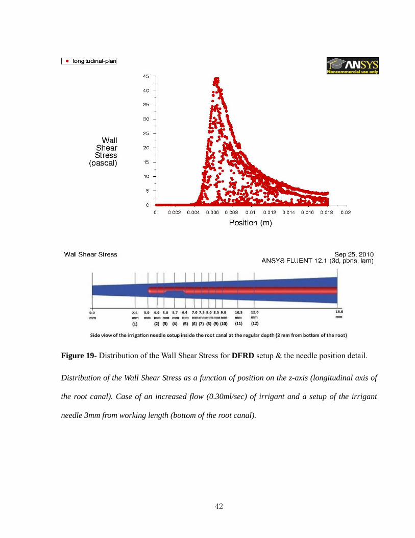
Figure 19- Distribution of the Wall Shear Stress for DFRD setup & the needle position detail.


the root canal). Case of an increased flow (0.30ml/sec) of irrigant and a setup of the irrigant

needle 3mm from working length (bottom of the root canal).

42

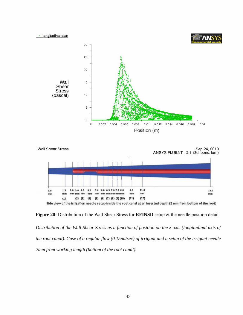
Figure 20- Distribution of the Wall Shear Stress for RFINSD setup & the needle position detail.


the root canal). Case of a regular flow (0.15ml/sec) of irrigant and a setup of the irrigant needle

2mm from working length (bottom of the root canal).

43

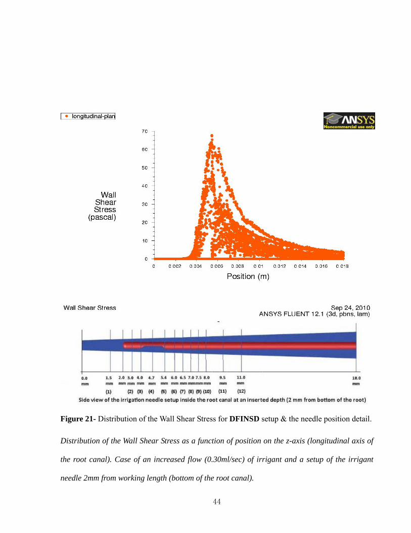
Figure 21- Distribution of the Wall Shear Stress for DFINSD setup & the needle position detail.


the root canal). Case of an increased flow (0.30ml/sec) of irrigant and a setup of the irrigant

needle 2mm from working length (bottom of the root canal).

44

Velocity magnitude (m/s)

Location (i) Location (ii)

Location (iii)

Figure 22- Contours of velocity vectors at the irrigant needle vent for the RFRD setup.

45



Location (iii)

Figure 23- Contours of velocity vectors at the irrigant needle vent for the DFRD setup.

46



Location (iii)

Figure 24- Contours of velocity vectors at the irrigant needle vent for the RFINSD setup.

47



Location (iii)

Figure 25- Contours of velocity vectors at the irrigant needle vent for the DFINSD setup.

48

section (1) section (2) section (3) section (4)

Section(5) section(6) section(7) section(8)

section(9) section(10) section(11) section(12)

Figure 26- Comparison of the velocity magnitude at RFRD setup condition.

49

section (1) section(2) section(3) section(4)



Figure 27- Comparison of the velocity magnitude at DFRD setup condition.

50




Figure 28- Comparison of the velocity magnitude at RFINSD setup condition.

51




Figure 29- Comparison of the velocity magnitude at DFINSD setup condition.

52

Contour of the velocity magnitude Contour of the velocity magnitude at the irrigant needle vent-RFINSD setup at the irrigant needle vent-RFRD setup

Contour of the velocity magnitude Contour of the velocity magnitude at the irrigant needle vent-DFINSD setup at the irrigant needle vent-DFRD setup

Figure 30- Comparison of the velocity magnitude at the exit of the side vent at 4 setup conditions

53

References

1. Falk, Kenneth W., and Sedgley, Christine M., “The Influence of Preparation Size on the

Mechanical Efficacy of Root Canal Irrigation in Vitro” JOE—Volume 31, Number 10, October

2005.

2. Usman, Najia, Baumgartner J. Craig, and Marshall, J. Gordon “Influence of Instrument

Size on Root Canal Debridement”, JOE— Volume 30, No. 2, February 2004.

3. Factsheet compiled by the Academy of General Dentistry-“What is a Root Canal?”

Featured in Oral Health Resources, Root Canal, March 30, 2007.

4. Buchanan, L. Stephen, “Managing Severe Canal Curvatures and Apical Impediments: An

Endodontic Case Study”, April 2005.

5. Boutsioukis, C., Lambrianidis, T., & Kastrinakis, E. “Irrigant flow within a prepared root

canal using various flow rates-a CFD study”, International Endodontic Journal, 42, 144–155,

2009.

6. Vinothkumar,Thilla Sekar, Kavitha, Sanjeev, Lakshminarayanan,

Lakshmikanthanbharathi, Gomathi, Narayanan Shivaram, and Kumar, Vanaja “Influence of

Irrigating Needle-Tip Designs in Removing Bacteria Inoculated Into Instrumented Root Canals

Measured Using Single-Tube Luminometer”, JOE—Volume 33, Number 6, June 2007.

7. Haapasalo, Markus, Shen, Ya, Qian, Wei, Gao, Yuan “Irrigation in Endodontics“, Dent

Clin N Am 54 (2010) 291–312.

8. Shen, Ya , Gao, Yuan, Qian, Wei , Ruse, N. Dorin, Zhou, Xuedong, Wu, Hongkun, and

Haapasalo, Markus “Three-dimensional Numeric Simulation of Root Canal Irrigant Flow with

Different Irrigation Needles”, JOE — Volume 36, Number 5, May 2010.

9. Bhaskaran, Rajesh and Collins, Lance “Introduction to CFD Basics”.

54

10. ”The Focus”, Publication for ANSYS Users”Tet-Meshing” ANSYS vs. ICEM CFD-April

25, 2002.

11. ANSYS Fluent 12.0 Getting Started Guide, April 2009.

12. Khademi, Abbasali, Yazdizadeh, Mohammad, and Feizianfard, Mahboobe,

“Determination of the Minimum Instrumentation Size for Penetration of Irrigants to the Apical

Third of Root Canal Systems”, JOE — Volume 32, Number 5, May 2006.

13. Boutsioukis, C., Verhaagen, B., Versluis,M., Kastrinakis, E. & L. W. M. van der Sluis,

Lucas“Irrigant flow in the root canal-experimental validation of an unsteady CFD model using

high-speed imaging”, International Endodontic Journal, 43, 393–403, 2010.

14. Boutsioukis, Christos, Verhaagen, Bram, Versluis, Michel , Kastrinakis, Eleftherios ,

Wesselink, Paul R., and W.M. van der Sluis, Lucas “Evaluation of Irrigant Flow in the Root

Canal Using Different Needle Types by an Unsteady Computational Fluid Dynamics Model”,

JOE — Volume 36, Number 5, May 2010.

15. McCabe W.L., Smith J.C., Harriott P.” Unit Operations of Chemical Engineering”, 7th

ed. New York, USA: McGraw-Hill, 2004, pp. 45–67, 98–132, 244–98, 929–65.

16. Azuma T., Hoshino T. “The radial flow of a thin liquid film”, Bulletin of Japan Society

of Mechanical Engineers 28, 1682–9. (5th report, influence of wall roughness on laminar-

turbulent transition).

17. Gao, Yuan, Haapasalo, Markus, Shen, Ya, Wu ,Hongkun, Li, Bingdong, Ruse, N. Dorin,

and Zhou, Xuedong, “Development and Validation of a Three-dimensional Computational Fluid

Dynamics Model of Root Canal Irrigation”, JOE — Volume 35, Number 9, September 2009.

18. Yuan Ling Ng BDS (HK), MSc (Lond), MRD RCS (Lond) “Factors affecting outcome of

non-surgical root canal treatment”, A thesis for the degree of Doctor of Philosophy, University

College London, and University of London.

55

56

19. Qingxi, Hu, Chenxia, Song, Yuan, Yao, Qi, Lu, “Computer-Aided analyzing system in

root canal therapy”, Rapid Manufacturing Engineering Center, Shanghai University, Shanghai

200444, P. R. China.

20. Muller, M., Schirm, S., Teschner, M., Heidelberger, B., Gross, M., ETH Zurich,

Switzerland “Interaction of Fluids with Deformable Solids”.

Root Canal Irrigation- An engineering analysis using Computational Fluid … · ·...

Documents

Transcript of Root Canal Irrigation- An engineering analysis using Computational Fluid … · ·...