Robust Nonlinear Feedback Control of Aircraft Propulsion ... · Robust Nonlinear Feedback Control...
122
FINAL REPORT Robust Nonlinear Feedback Control of Aircraft Propulsion Systems NASA Glen Research Center Grant: NAG-3-1975 SUBMITTED TO: NASA Glen Research Center Attention: Grants Office 21000 Brookpark Road, Mail Stop 500-319 Cleveland, OH 44135-3191 NASA TECHNICAL OFFICER: Jonathan Litt NASA Glen Research Center 21000 Brookpark Road, MaiI Stop 77-1 Cleveland, OH 44135-3191 216.433.3748 15 JANUARY, 2001 Principal Investigators: Contract Dates: Total Budget: Drs. William L. Garrard and Gary J. Balas Department of Aerospace Engineering and Mechanics University of Minnesota Minneapolis, MN 55455 612.625.8000 wgarrard, balas_aem, umn. edu 1 November 1996 - 30 January 2001 $ 204,848 https://ntrs.nasa.gov/search.jsp?R=20010011959 2020-02-20T20:33:37+00:00Z
Transcript of Robust Nonlinear Feedback Control of Aircraft Propulsion ... · Robust Nonlinear Feedback Control...

FINAL REPORT
Robust Nonlinear Feedback Control of
Aircraft Propulsion Systems
NASA Glen Research Center Grant: NAG-3-1975
SUBMITTED TO:
NASA Glen Research Center
Attention: Grants Office
21000 Brookpark Road, Mail Stop 500-319
Cleveland, OH 44135-3191
NASA TECHNICAL OFFICER:
Jonathan Litt
NASA Glen Research Center
21000 Brookpark Road, MaiI Stop 77-1
Cleveland, OH 44135-3191
216.433.3748
15 JANUARY, 2001
Principal Investigators:
Contract Dates:
Total Budget:
Drs. William L. Garrard and Gary J. Balas
Department of Aerospace Engineering and Mechanics
University of Minnesota
Minneapolis, MN 55455
612.625.8000
wgarrard, balas_aem, umn. edu
1 November 1996 - 30 January 2001
$ 204,848
https://ntrs.nasa.gov/search.jsp?R=20010011959 2020-02-20T20:33:37+00:00Z

Abstract
This is the final report on the research performed under NASA Glen grant NASA/NAG-
3-1975 concerning feedback control of the Pratt & Whitney (PW) STF 952, a twin spool,
mixed flow, after burning turbofan engine. The research focussed on the design of linear
and gain-scheduled, multivariable inner-loop controllers for the PW turbofan engine using
Hoo and linear, parameter-varying (LPV) control techniques. The nonlinear turbofan engine
simulation was provided by Pratt & Whitney within the NASA ROCETS simulation soft-
ware environment. ROCETS was used to generate linearized models of the turbofan engine
for control design and analysis as well as the simulation environment to evaluate the perfor-
mance and robustness of the controllers. Comparison between the 7-/o_ and LPV controllers
are made with the baseline multivariable controller and developed by Pratt & Whitney en-
gineers included in the ROCETS simulation. Simulation results indicate that N_ and LPV
techniques effectively achieve desired response characteristics with minimal cross coupling
between commanded values and are very robust to unmodeled dynamics and sensor noise.

Chapter 1
Introduction
The design of traditional gain-scheduled, inner-loop controllers for a turbofan engine takes
significant time and can not guarantee performance and stability of the closed-loop system
across the operating envelope [10]. Linear parameter-varying (LPV) control methodologies
can however, guarantee stability and performance over the entire operating envelope, making
them a natural approach for inner-loop control of turbofan engines. This report documents
the application of LPV control design techniques to a PW turbofan engine. Pratt & Whitney
and NASA Glenn at Lewis Field Research Center provided the University of Minnesota with
a transient turbofan engine simulation (ROCETS) to use as a test bed for implementing LPV
control designs. The baseline multivariable control algorithm in ROCETS was implemented
as many interconnected subroutines rather than as a single integrated subroutine. This was
not conducive to implementation and simulation of candidate controllers, and necessitated
changes to the controller software implementation in ROCETS. This report discusses the
revisions required to implement state-space and LPV controllers, the design of 7-/oo and LPV
controllers, and the results obtained from the implementation of the controllers in the Pratt
& Whitney engine simulation.
1.1 Accomplishments
This grant partially supported the turbofan engine control research of Professors Gary Balas
and William Garrard, a post-doctoral researcher, Dr. Greg Wolodkin, two graduate students,
Jack Ryan and Dr. Jeff Barker, and two undergraduate researchers, Chris Mitchell and
Edward Harper. Dr. Wolodkin currently works at the Mathworks and was one of their lead
engineers in the advanced controls area. He has since moved within the Mathworks and

is currently responsiblefor the core Matlab product. Dr. Barker graduated with the Ph.D.degreein 1999and is employedby BoeingPhantomWorks in St. Louis. JackRyan wrote hisMaster's project report on the turbofan engineresearchand is currently employedby NASADryden Flight ResearchCenter as a flight simulation engineer. (Note that Chapters 2, 3and 5 of this report are based,in part, on his Master's report.) Chris Mitchell is currentlya Ph.D. student in the AerospaceEngineeringand Mechanicsdepartment at the Universityof Minnesota in fluid mechanicsand Edward Harper is currently working as an engineerinindustry.
The following area list of the technicalaccomplishmentsachievedwith the support of thisgrant.
Learnedto usethe NASA RocketEngineTransient Simulation (ROCETS) systemtosimulate the turbofan enginemodel provided by Pratt and Whitney (PW).
Developmentof a linear, parameter-varying(LPV) model of the PW turbofan enginefor control design.
Developedand integratedFortran subroutinesto implementlinear andLPV state-spacecontrollersinto the ROCETS nonlinearsimulation.
Successfullybackengineeredthe baselinePW multivariable controller.
Synthesizedrobust, linear multivariable 7-/o_controllersand gain-scheduledLPV con-troller for the turbofan engine.
Successfullyimplementedthesecontrollersin the ROCETS nonlinearsimulation.
Achievedperformancerobustnessof the non-rate and rate boundedLPV controllers.The LPV controllerswere scheduledon a laggedmeasurementof power code. Thesecontrollersperformedwell for a variety of environmentalconditions, through the flightenvelopewith and without noisy sensormeasurements.
Three papersand a Mastersproject report werewritten on the synthesisof controllers forturbofan engineduring the length of this contract. A fourth paper is in preparation basedon the latest resultsof the gain-scheduledLPV inner-loop controllers for the PW turbofanenginemodel. The technicalmonitor for this grantwasJonathanLitt, NASA Glenn ResearchCenter.
• G. Wolodkin, G.J. Balas,W.L. Garrard, "Application of parameter-dependentrobustcontrol synthesisto turbofan engines,' AIAA Journal of Guidance, Dynamics and
Control, vol. 22, no. 6, 1999, pp. 833-838.
4

,, G. Wolodkin, G.J. Balas, W.L. Garrard, "Application of Parameter-Dependent Robust
Control Synthesis to Turbofan Engines," 36th AIAA Aerospace Sciences Meeting, Reno,
NV, January, 1998, AIAA-98-0973.
• G.J. Balas, J. Ryan, J.Y. Shin, W.L. Garrard, "A New Technique for Design of Con-
trollers for Turbofan Engines," 3dth Joint Propulsion Conference, Session 95-ASME-21,
Cleveland, OH, July, 1998, AIAA-98-3751.
Chapter 2
Engine Simulation
The Pratt & Whitney STF 952 (Figure 2.1), a twin spool, mixed flow, after burning turbofan
engine, is used as the example application in this study. It features a highly loaded, three
stage fan, a four stage high pressure compressor, an axially staged triangular alignment
combuster, and an advanced high pressure turbine and low pressure turbine. For later
reference, the fan inlet is identified as station 2, the high pressure turbine inlet as station 4,
and the turbine exit guide vane as station 6. The pressures at each station are designated as
P2, P4, and P6 respectively. A diagram of the engine and the actuator and sensor locations
is given in Figure 2.1.
The STF 952 engine is modeled using the NASA Rocket Engine Transient Simulation
(ROCETS) software. The ROCETS model of the STF 952 engine is fully nonlinear and it
uses a multivariable integration routine based on a modified Newton-Raphson technique to
calculate transient responses and steady-state balance. The linearized models of the STF
952 engine are all generated using ROCETS as are all nonlinear closed-loop simulations.
Through out this report, we will denote the PW STF 952 turbofan engine as the "engine"
or "turbofan engine" in the text.
The engine dynamics vary with thrust request or "power code," temperature and external
air pressure. Air pressure and temperature vary with altitude as well as weather. The
engine power code varies from 3,000 to 30,000 which corresponds to near idle to military
power. Initially, the altitude is set at sea level, OK ft, a speed of zero Mach and standard
atmosphere. The objective of the control system is to accurately track inner-loop commands
to the engine.
A turbofan engine transient performance computer model of the SCIP Engine (STF 952A)
was configured using the NASA Rocket Engine Transient Simulation (ROCETS) system.

ROCETS interfaces modular components to generate a full engine simulation in which a run
processor reads and interprets input to run particular experiments. A multi-variable modified
Newton-Raphson technique is used for transient integrations and steady-state balances [1]
Schedules of desired thrust level, altitude, Mach number, or other variables can be input
to the simulation. The simulation model of engine dynamics generate the necessary overall
pressure ratio (OPR = P4/P2), engine pressure ratio (EPR = P6/P2) and high pres-
sure compressor spool speed (N2) requests to meet the scheduled variables. These requests
(OPRREQ, EPRREQ, N2REQ) are fed to the inner-loop control system which generates the
required primary burner fuel flow (WFPRIB), high pressure compressor normalized variable
vane angle (VANEHPC), and convergent throat area (AREANOZL) commands to achieve
the requests. This control inner-loop is the focus of this report.
The current multivariable controller in the turbofan simulation, used as a baseline to com-
pare with designed controllers, operates in two modes: start mode and nominal multivariable
mode. The start mode is used to transition from light off fuel flow, to nominal multivariable
control mode. The nominal multivariable mode uses a controller scheduled on total corrected
airflow [1]. This paper focuses on the design of a controller for the nominal multivariable
mode. The baseline controller is used during the initialization part of the simulation.
The baseline control interconnection (Figure 2.2) has an two loops.
o
Fan
, ,
_ Burner
a5 _s2 1.3 2.5 3 4 4.5
/
0_z
6 7 8
Figure 2.1: STF 952 Turbofan Engine
The inner control loop consists of the state space matrix K and the gain matrix S. The K

P H
I_ X
req
Figure 2.2: Interconnection of Engine Model and Baseline PW Controller
matrix has the form
K
where
0 1 0 0
A2,1 1 -- A2,1 A2,3 -A2,3
0 0 0 1
A4,t -A4,1 A4,3 1 - A4,3
As,t -As,, A5,3 -A5,3
0 1 0 0
0 0 0 1
As,, -A5,1 A5,3 -A5,3
0 0
0 0
0 0
0 0
1 0
0 St,,
0 $2, l
1 $3,1
0 0 B1,1 B1,2 B1,3
0 0 B2,1 B2,2 B2,3
0 0 B3,1 B3,2 B3,3
0 0 B4,1 B4,2 B4,3
0 0 B5,1 B5,2 B5,3
$1,2 S1,3 0 0 0
S2,2 $2, 3 0 O 0
$3,2 $3, 3 0 0 0
(2.1)
St,, = Bt,, + D1,1
$2,1 = B3,1 + D2,1
S3,t = B5,1 + D3,1
S1,2 = B1,2 + D1,2
$2,2 = B3,2 + D2,2
Sa,2 = Bs,2 + D3,2
$1,3 = Bt,3 + D1,3
$2,3 = B3,3 + D2,3
$3,3 = B5,3 + D3,3
(2.2)
The values of A+j, Bi,j, Di,j are determined via a look-up table scheduled on operating
condition. The states of the controller are: gas generator fuel flow (xl), precursor to the
normalized gas generator fuel flow (x2), normalized flow parameter(x3), precursor to the
normalized flow parameter(x4), and normalized compressor variable vane(xs).
The inputs to K are
U-_-[ _/'1 ?22 _3 IT (2.3)
and
e=[el e_ e3 ] T (2.4)
8

u consistsof normalizedoverall pressureratio error (ul), normalizedengine pressureratioerror (u2), and normalized rotor speederror (u3). The vector e consists of overall pressure
ratio error from the last pass through the loop (el), engine pressure ratio error from the last
pass through the loop (e2), and high rotor speed error from the last pass through the loop
(e3).
The outputs from the controller are
z=[xl z4 (2.5)and
v = [ y, y2 y3 (2.6)
Yl is normalized fuel flow request, Y2 is normalized flow parameter request, and Y3 is nor-
malized compressor variable vane request.
The S matrix has the form
1 $2,2S3,3 -- $3,2S2,3 $3,2S1,3 - S1,2S3,3 S1,2S2,3 - $2,2S1,3
DETGN $3,1S2, 3 - $2,1S3, 3 S1,1S3, 3 - S3,1S1, 3 $2,1S1, 3 - S1,1S2,3 (2.7)
&,lSa,2 - $3,,&,2 $3,,$1,2 - &,,$2,1 $1,,$2,2 - $2,,$1,2
where
DETGN = SI,ISe,2Ss,3 + 31,232,3S3,1 + $2,3S2,1S3,2 - S3,1S2,eSI,s - Ss,2S22S_,1 - $3,3S2,_S_,e
(2.8)
It has inputs Yl - xl, Y2 - x4,and Y3 - xs, and outputs el, e2, and e3. Together, K and S
form the baseline controller for inner-loop control of the PW turbofan engine.
The closed-loop system consists of the plant model (P), two constant gain matrices (OSC
and ISC), and the controller. The outer-loop control generates the desired values of overall
pressure ratio (OPRREQ), engine pressure ratio (EPRREQ), and high speed rotor request
(N2REQ) based on environmental conditions, power code and the baseline closed-loop engine
dynamic response.
The inputs to the plant, P in Figure 2.2, are WFPRIB, VANEHPC, and AREANOZL. The
plant outputs are P2, P4, P6, and N2. The matrix OSC normalizes its inputs from overall
pressure ratio error (OPRREQ-OPR), engine pressure ratio error (EPRREQ-EPR) and high
rotor speed error(N2REQ-N2) to the normalized parameters ul,u2, and u3. The matrix ISC
dimensionalizes its inputs from yl, y2, and Y3 to WFPRIB, AREANOZL, and VANEHPC.
The ISC gain matrix is
7 0 0
0 807 0 (2.9)
0 0 1
9

and the OSC gain matrix is
o.0320491 0 014.55
0 0.1599723 014.55
0 0 0.000055528
(2.10)
2.1 Controller Subroutines
To implement state-space multivariable controllers, changes were required to the ROCETS
nonlinear simulation of the turbofan engine model. These modifications allow 3 input, 3
output multivarible controllers of state order up to 21 to be read in and replace the baseline
Pratt & Whitney controller. This allowed controllers to be easily tested in the simulation
without rewriting or recompiling the ROCETS simulation. Changes were also made so that
the simulation uses the Pratt _z Whitney controller in the start up mode until it has reached
the multivariable control mode. This eliminates engine start-up issues in the design of 7/o_
and LPV controllers.
The new code reads in the synthesized controller at the beginning of each simulation. If the
controller has less than 21 states, it is padded with zeros so that the multiplication routine
only need work with a constant size control matrix. Figure 2.3 shows the implementation of
a five state controller in the control algorithm. The usual ABCD five state control matrix
is located in the bottom right corner. Zeros fill the remaining entries keeping Xl through x16
constant zeros. Details of the algorithm are presented in Appendix B.
The ROCETS state-space controller implementation was tested with the Pratt & Whitney
baseline controller and the results were compared with the original simulation of the PW
baseline controller implementation. This was necessary to demonstrate our understanding of
the existing code and our ability to replace the control algorithms with out jeopardizing the
overall engine simulation. The baseline simulation matched well with the new implementa-
tion verifying the state-space algorithms. Figure 2.4 compares the Pratt & Whitney control
inputs and outputs with our implementation of the Pratt & Whitney controller. Pratt &
Whitney's N2 follows its request ramping up after the step input while our implementation's
N2 follows its request which does not ramp up. The difference is due to the reference com-
mand request generating algorithm which is not part of this research project. EPR, OPR
and N2 commands are treated as exogenous inputs in the control problem since we do not
have direct control of them. The differences in VANEHPC are directly due to the variations
in the N2 commands. The small variations in the other channels are not significant.
10

Xl,
XL6
Xl7XL8 --
Xl9
X2o[
Xzll
Y:Y?
00 ...0 0
• .
00 ...0 0
0 0 A11 A120 0 A21 A220 0 A31 A320 0 A41 A42
0 0 A51 A520 0 Cll C12
0 0 C21 C22
0 0 oo. C31 C32
0 0 0 0
0 0 0 0
A15 Bll Blz Bt3A25 B21 B22 B23A35 B31 B32 B33A45 B41 B42 B43A55 B51 B52 B53
C15 Dll D12 D13
C25 D2_ D22 D23
C3s D31 D32 D33
Figure 2.3: Five State Controller in 21 State Framework
Xl
• XL_
Xt_
Xzc
X21
UtU_U3
11

163 c
UM Im_l_nlOd Ovo r_ll Ptl l,lllJrl RabO (pc= 15k ÷ 100 ll_f llopl
16 2
le _5o
ii 20
PW
- - - PWREQ
UM Imp
UM Imp REQ
25
UM Imp_m'4mt4_ Err_r_l P_l_nl Rabo (pc=lSk + IC_ Ibf i1_0)
2 7_
2 7S
2 78E
2 ?e
2 7?
2 76E
2 75_
r
J_ ......................
d,l
- - - PWREQ
UM Imp
2'5 3o
g
Tim_mec)
lO4 UM Impilm_l_tlKI H_ ROlOr _ (pc= 15k + 100 IN itllp)
....... -- Pw !,, - - PwREQ II UM trrO REQr
286
285
2B4
283
2_2
_28_
28
279
2 78
I II- - UM _mp
20 25 3C
T,m,e,(xcl
UM _mp_e,,'_mre_ Sp_w_ Con_rga_ Fmp Nozze_ Arm=
' ' PW
445 _ t
_o,2!
T_(leCt
UM Impi_t_ H_ Pt_uurll C_t No ml_l_zed Vm_ Var_ P OII_K_I
•-OOaS F
O04 P
I--- ;;'"_ I
Tin141( lime ) T,m4Htec)
Figure 2.4: UM implementation of PW Baseline Inner-loop Controller
12

2.2 Engine Linearized Models
Ten Jacobian linearized plant models were generated using the nonlinear simulation between
3000 and 30000 lbf thrust at 3000 lbf thrust intervals and different altitudes. Each model was
generated for a given altitude, zero Mach, zero angle of attack, standard atmosphere, zero
side slip, and 14.696 psi static pressure. The Jacobian linearizations have 11 states, three
inputs, and three outputs. The states are identified in Table 2.1, the inputs in Table 2.2,and
the outputs in Table 2.3. The simulation's input file used to generate the linear plants along
with Matlab utilities to move the generated plants into Matlab files are provided in Appendix
A.3 and A.A.4.4 respectively.
State Description
SN1 Low Rotor Physical Speed (rpm)
TMCHPC High pressure compressor case lumped metal temperature (deg R)
TMBHPC High pressure compressor blade lumped metal temperature (deg R)
TMRHPC High pressure compressor rotor lumped metal temperature (deg R)
TMCHPT High pressure turbine case lumped metal temperature (deg R)
TMBHPT High pressure turbine blade lumped metal temperature (deg R)
TMRHPT High pressure turbine rotor lumped metal temperature (deg R)
TMCLPT Low pressure turbine case lumped metal temperature (degR)
TMBLPT Low pressure turbine blade lumped metal temperature (degR)
TMRLPT Low pressure turbine rotor lumped metal temperature (deg R)
TMILBN Main burner liner metal temperature (deg R)
Table 2.1: Linear Plant States
Input Description
WFPRIB Primary Fuel Flow rate (lbm/sec)
VANEHPC High pressure compressor normalized variable vane position
AREANOZL Spherical Convergent flap nozzle physical area (in 2)
Table 2.2: Linear Plant Inputs
Figure 2.5 shows the magnitude and phase of the linearized plants. The dotted line repre-
sents the 3000 lbf model, the solid 15000 lbf model, and the dash-dot line 30000 lbf model.
All other power codes are represented by the dash lines.
The linearized engine models are used for the 7-/o_ and LPV control designs. The plots in
Figure 2.5 indicate that the state order of these models may be reduced. Balanced realization
13

Output Description
P2 Engine facetotal pressure(psi)P4 Primary burner exit total pressure(psi)P6 Turbine exit guide vane exit total pressure (psi)
N2 High rotor physical speed (rpm)
Table 2.3: Linear Plant Outputs
model reduction will be used to reduce the plant state order. Since the LPV design model
requires all states to have the same meaning, the same balancing transformation matrix
must be used for all plant models. The transformation matrix at the 12,000 power code was
selected to balance the models. After balancing, all engine models were truncated to three
states with no effect on the plant dynamics.
14

Plant Model MagnitudeWFPRIB AREANOZL VANEHPC
....... 1 '°°l_....... 1°'I 101 10-3L J 10 -2
10-2 10 o 102 10 -2 100 102 10 .2 100 102
101 .......
_. _10010- -:- - _
I0 -2 10 0 I0 z
ooi10 -_
10 "2 -i 10 -2l I
10 -z 10° 10 2 10-2 100 10 2
1041 2 _._ } 10_ _ -- --
_1o' : 1°° ..... "
I02L I 1041 I
10 -2 100 102 10-; 100 102
104 1 .... 1
1o_I_;-i_=- _---i- ==- E-
102/ , ]
10-2 10o 10;
WFPRIB
10 -2 100 102
I0 "2 100 102
15 // _
10 "2 100 102
Plant Model PhaseAREANOZL VANEHPC
0 '., !
10 -2 100 102
-100[
2{ :i°°I.....10-2 100 102 10 -2
0 _¸_ i ,'7---
10-z 10° 102
1O
-100 l-200
10 -z
I0 "2 100 10 z
10 0 10 2
Figure 2.5: Magnitude (top) and Phase (bottom) of Jacobian Linearizations at Sea Level
and Standard Day Atmosphere.
15

Chapter 3
Controllers
7-/_ control design techniques are used to synthesize controllers for the PW turbofan at ten
power code operating points. Jacobian linearizations of the turbofan engine were generated
at power codes from 3000 to 30000 lbf thrust in 3000 lbf increments. The reader is referred
to references [18, 13, 16] for details on _ control theory and its application. The con-
trol objectives were to achieve good tracking of OPR, EPR, and N2 commands, decoupled
command response, disturbance rejection below 2 rad/sec and a 10 rad/sec bandwidth and
robustness to modeling error, sensor noise and changing environmental conditions. The 7-/_
controllers also must respect the physical limits on the actuator deflections and rates. The
controllers are designed using a model matching problem formulation in the 7-/_ framework
(see Figure 3.1). We desired the engine to respond as three single-input/single-output (SISO)
systems with no off-diagonal coupling. Pmod represents the decoupled system. Differences
between this desired model and the true plant are penalized via the weight Wp.
The disturbance vector dl represents customer demands, whose values we wish the plant
output to track. Specifically these commands correspond to desired normalized overall en-
gine pressure ratio, normalized engine pressure ratio and normalized high rotor speed. The
disturbance vector d2 is used to represent both noise and input uncertainty in the problem
fornmlation to which the controller should be robust. The input uncertainty is mapped to
tile output of the plant model to reduce the number of states required to define the open-loop
control design interconnection.
By keeping the error vector el small, good tracking of dl is ensured. The role of e2 is
to penalize control effort, in terms of actuator magnitudes as well as actuator rates. The
controller sees Yc as its input measurements, and generates uc as its output.
16

The actuators aremodeledas P_ct, a diagonal augmentation of unity gain first-order lags,
100P,_a - --I3×3 (3.1)
s + 100
The actuator model outputs actuator positions u and actuator rates _2, to allow actuator
rates to be penalized in the control design.
The model-matching block Pmod was based on previous work in Reference [2]. It is desired
that the engine response to OPR and .EPR request follow a second order model with natural
frequency of 10 rad/sec and damping of 0.65. The engine response to N2 request should
follow a second order model with natural frequency of 2.5 rad/sec and damping of 0.65.
Pmod, S 2 + 2_Wi q- W2i
Pmodl 0 0
0 Pmodl 0
0 0 Pmo,h
Here aq = 10 rad/s, co2 = 2.5 rad/s, and _ = 0.65.
The input weight Wi is a constant weighting used to normalize the inputs.
weight
The input
0.08 0 0
0 0.06 0
0 0 0.25
in these designs.
The disturbance Wd is used to model actuator errors as well as limit the bandwidth of
control effort by ramping up at high frequency.
Wd = 0.0005 °1-7s + 1 /ax3,1
a--ff_s + 1
The control weights Wc are selected to be constant. Here we have chosen to penalize the
normalized actuator movement larger than unity, as well as actuator rates,
VV rC
0.05 0 0 0 0 0
0 0.02 0 0 0 0
0 0 0.05 0 0 0
0 0 0 0.05 0 0
0 0 0 0 0.005 0
0 0 0 0 0 0.05
17

The performance weight Wp penalizes the difference between the desired and the actual
closed-loop response of the turbofan engine. The larger the magnitude of Wp, the smaller
the allowable difference between desired and actual output. In the initial designs, _ is a
first order low-pass weight given by
W_
....!---_,+ 1500_ 0 0
_-_s+l
300" £_ s+ao _ 0
.... l_s+l
0 0 4oo_
This ensures good tracking of the response models in the bandwidth 1-10 rad/s, with little
or no DC error. At low frequency (below 0.1 rad/s) the Wp weight on the OPR corresponds1 1
to a DC errors of _ or 0.2% tracking error. The EPR tracking error at DC is a--N or 0.33%1
and the N2 tracking error at DC can be ag6 or 0.25%. At high frequency, the mismatch
between actual and desired output is not penalized.
The matrix OSC normalizes its inputs from overall pressure ratio error (OPRREQ-OPR),
engine pressure ratio error (EPRREQ-EPR) and high rotor speed error(N2REQ-N2).
d_
P,noa _ dl
Figure 3.1: 7-/o_ control design interconnection
The open-loop interconnection shown in Figure 3.1 has 18 states. Hence the resulting con-
trollers had 18 states. Eight of the ten 7-t_ point designs at the power codes between 3K and
30K achieved an 7-/_ norm less than 1.62 and all ten were under 2.4. They were first tested in
linear simulations and then in the nonlinear ROCETS simulation for small step commands.
While the linear simulations were satisfactory, the nonlinear simulation resulted in highly
oscillatory reference commands. Recall that the reference commands are generated by an
outer-loop controller which has not been modified from the original PW baseline design.
18

Figure 3.2 and 3.3, showthe ROCETS simulation time responsewith a linear7-t_ controllerimplementand a step commandfrom 15000lbf to 15100lbf. The simulation-generatedcom-mandsof OPR,EPR, and N2 areall oscillatoryresulting in oscillatory responses.Controllersdesignedfor the other nine powercodeshad similar results.
19

IB25
162
6 15
161 .........
_f105
1%--
28
2 795
279
2 785
OVl_tall PrlNauro Palio (pc=l 5k + 1CO _1 SlI:_)
t_
tl
fl
f I
[
i
i
ql
Time(a4K:)
En_ipe P_ure RalK_ (pc=lSk ÷ _00 Ibl IIIOp)
PW
- - - PW REQ
--- UM
UM REQ
278 I "'_tIJ
277 .......... _
2 765
276
)2 755
27-1 $ 20 25
X 10 _ P_ P_oIor _oe41d (pc=t Sk ÷ 100 II>f IdIO)
I 606 , PW |
h - - - PW REQ !I_ _ UM |
_ *1 UM REQ J
.¢"5
1602 il
's_ _ _Time(sec/
Figure 3.2: Controller Inputs of 7/00 Controlled System
20

2 86
Plant Ir_ul Pnr_ary Fuel _low Pale
285
284
283
g
_m
_281
28
2 79
2 78
2 7_
15
448
I
I II iir
I rl i I
I _ I l I
' t J I j _ IL /'
I t Ib I t I J
i i II r II %I r I i
I I I _ II
I I Ip
Ip _j
i I i_
_P
I L
2O 25
Tirr_(_)
Plant Inpu_ Sphencal Cofwergant Flap Nozzel A_0a
r i_ t
443 I I
Tirne(sec)
Plant IP,put High I_r_auro Co_re_ll_or Normalized Van&hie Vane Polltion
*0 082
-0084
-0 086
-0088
-009
_ -0 O92
-0 O94
-0 096
-0 098 ...........
-0 t
r_
q
t_ _ _ r _ _ _ • •
15 _ 2_5 30
Figure 3.3: Plant Inputs of 7-{_ Controlled System
21

3.1 Identification of Linear Engine Models
Tile good performance of the _o_ controllers on the linear engine models and the poor
performance of these controllers in the nonlinear simulation required investigation. The first
hypothesis was an error in the implementation of the linear state-space controller subroutine
in ROCETS. After testing, it was found that this was not the case. Therefore, the problem
must have been related to the inaccuracy of the linearized engine model relative to the
nonlinear engine simulation. This could be due to several reasons. The first is our poor
understanding of the ROCETS simulation code. Hence we may have incorrectly linearized
the engine. Similarly, the ROCETS linearization may only include engine dynamics and
therefore all the actuator and sensor dynamics, as well as filtering and computational delays
need to be included in the linear engine model as well. The linear models used in the
controller synthesis did not capture all the nonlinear plant dynamics. These unmodelled
dynamics, we conjectured, were causing the oscillations. The linear and nonlinear responses
of the plant to single channel inputs were therefore examined.
The nonlinear ROCETS simulation needed to be modified since it was not designed for
such an examination. By setting two of the three controller outputs to zero, the remaining
plant input could be set to a variable frequency sinusoidal. Figure 3.4 shows the responses
to the single sinusoidal inputs. The nonlinear simulation response is represented by the solid
lines, and the linear models response by the dashed lines. In each set of plots, the top left
plot displays the active input signal: WFPRIB in the first, AREANOZL in the second, and
VANEHPC in the third. The remaining plots display the signal responses of OPR, EPR, and
N2. We can see that the linear and nonlinear models do not match exactly. In particular, the
nonlinear responses of N2 are smoother than their linear counterparts. They respond slower
and subsequently lack the sharp overshoot. After examining all the controller inputs and
outputs, to better match the nonlinear engine simulation: the actuator model was modified,
a sensor model added to the rotor speed sensor, N2, and a lag filter was included in the
high speed pressure compressor vane actuator, to help slow down the response of N2 and
compensate for the differences between the linear time response and nonlinear simulation.
The small signal simulations of the modified linear engine models matched the nonlinear
engine simulations well across power code at sea level and standard atmosphere. The new
actuator model was chosen as
22

Pact
20 0 0s+20
0 20 0s+20
0 0 15s+15
2o_ 0 0s+20
0 2o_ 0s+20
0 0 15_s+15
A sensor model was added to the N2 measurement,
_s+lsen -- 1
_s+l
and a lag filter was added to the N2 command channel,
lag - _s + 1_s+l
The modified linear engine models frequency responses are shown in Figure 3.5. The N2
phase change is apparent as is the VANEHPC input smooth roll off at high frequency. (See
Figure 2.5 for comparison.). The modified linear models of the engine are used to synthesize
all the subsequent 7/oo and LPV control designs.
23

28
2 798
_ 2.796
-_2794
2 782
279
WFPRIB
5 10 15
EPR
2 786
2.765
0:
_ 2764
2763
2762
t', ^t----
r I I iJl
J I d I i I
t •
0 5 10 15
Ti¢_(sac)
x 10' N2
1 8028 _ )L
16(320 t ! ri
1 602 I _ I r _z It
16018, i / iz_
16016 L
0 5 10 15
Tin_(sec)
413
412
_'E 411
410
400
/MqEANOZL
5 10 15
Single Varyin Input OPR
15 964_
0 5 10 15
292
2 915
291
2005
28
-0 0375
-0 037
_c-0 037
-0 0378
-0 0379
EPR
5 10
"rime(=,=cl
VANEHPC
5 10 15
EPR
X 10 4 N2
15808
15808 ,_
_ 1_ 5807 J _ L
_ q L_
_ 5805
15 _ 10 15
Single Varying Input oPR
1613 ---- t l /11 ,_ _-
I
1610 5 10 15
2 771
2 77
2 769
2 768
2 767
2 766 _
x 10" N2
1 5844
56_ _ _
1 88_7
5 !0 15 0 5 10 15
Time(sec} Time(sec i
Figure 3.4: Single Input Responses
24

WFPRIB
102; ....
=_ -:!_= _-- =_ - -
10 _10-2 10° 102
102
I01_
0.
I0°_10 -2 100 102
104 L_o_ 103 ....... " _,:""
I021 - -'1
10 .2 10 0 102
Plant Model MagnitudeAREANOZL VANEHPC
10° _ 1t0_ -----_ -- ---_10__ ..... - - -.._, 0o
,o-.I..... ,o-,I_.......10-3L J 10"2l J
10 .2 100 102 10-2 100 102
10° i ..... _7_'-=
-_I_:=:=:--::_ _ --'.-
lO --i- ----_
10_2F ............I0 -2 10 (J 102
10' I .,.....
10., _/_/_ ....
lO-Z_10 -2 100 102 10 -2 100 102
101
0 [ ....,._
lo l .......... --_.,, t
I0-_ .......
lO-Z/ ]
10 .2 10 o 102
'°'i 1lr)3[_= --- ;----i---- _,_':.\ !-I= =;_=_--_., I
r- - - _._.._ 1io,I _,.,.I
i0_I
WFPRIB
0 %
10 .2 10° 102
o.. -20[ _ 1
30i0 -2 100 10 2
0
co
-40
6O10 .2 100 102
Plant Model PhaseAREANOZL VANEHPC
0 \ 200 f- _ -- _ t.[ ,oo......-----1°°I .-->'_ 1
.o.-___>::-:,o°o 10 .2 100 102 10 -2 100 102
....1
-100_-200
10:f-300
10-2 10O 102 10 -2 100 102
100 150
- 100
oF--100 50L '
10 -2 100 102 10 -2 100 102
Figure 3.5' Magnitude (top) and Phase (bottom) of Modified Linear Engine Models with
Lag, Actuator and Sensor Models
25

3.2 Redesigned Controllers
The 7-/_ controllers were re-synthesized using the same weights as used in the original 7-/_
designs but with the new lag, sensor model and actuator model. The redesigned controllers
had 20 states and achieved a 7-/_ norm of 1.54. Time responses in the nonlinear ROCETS
simulation of the new 15000 lbf thrust system to a 100 lbf step are shown in Figure 3.7. The
oscillations in the reference commands have been eliminated. The 7-/_ controllers achieved
better tracking than the baseline controller in OPR and EPR, with comparable overshoot.
Note that with the 7-/o_ controller implemented in the nonlinear engine simulation, the re-
sponse of N2 exhibits more overshoot but better tracking of the N2 command as compared
with its baseline counterpart.
L Pact _ Uc
dl
Figure 3.6: 7-/_ control design interconnection
26

162
1615O
Overall Pressure RatK_ (pc=15k + 100 Ibf step}
PW
t - - - PW REQ
UM
16055 2(} 25
2.795
279
2785
278
2775
277
2.765
276
¢
I¸604
E
16_5¢
Time(see)
Engine Pressure RallO (pc=15k + 100 Ibf 11_)
PW
- - • PW REQ
UM
UM REQ
i
j t
r
It
.......... Ill
2755
27515 2(} 15 3(}
x 10 *1 605
Timelsec}
High Rotor Speed (pc=l 5k + 1GO Ibf step}
1 602£ 15 2(} 30
Q
k
k
PW
- - PW REQ
--- UM
UM REQ
Tirr_q_)
Figure 3.7: Controller Inputs of New 7-/o_ Controlled System
27

Chapter 4
Linear Parameter-Varying Control
Theory
We begin with a brief introduction to gain scheduling based on linear parameter-varying
representations. For a compact subset P C _s, the parameter variation set ._ denotes the
set of all piecewise continuous functions mapping 7_ (time) into P with a finite number of
discontinuities in any interval. A compact set P C 7_ s, along with continuous functions
A : TO.s --+ 7_n×_, B : 7-q2 -+ 7_"×_, C : 7__ --+ 7__e×_ and D : 7__ -+ _ne×nd represent an nth
order linear parametrically varying (LPV) system, whose dynamics evolve as
Ix(t)e(t) ] = [ A(p(t)) B(p(t))C(p(t)) D(p(t)) ] [ x(t)d(t) ] (4.1)
where p E _),. For here on the time dependence of the parameter p will be suppressed due to
space limitations. The induced 122 norm of a quadratically stable LPV system GT_, [5, 4, 7],
with zero initial conditions, is defined as
Hell,-IIG._ft- sup sup
peo:_, ]ldli2 _¢ 0 IIdll2
dcL2
This quantity is always finite.
rameter rate-of-variation problem can now be stated.
Consider a generalized )lant with the usual structure
2
el
g2
y
(4.2)
The quadratic LPV 7-performance with bounds on the pa-
A Bu B12 B2
Cn 0 0 0
C12 0 0 I
(72 0 I 0
X
dl
d2 '
?2
28

wherethe A, B, and C matrices are a function of p. For simplicity of derivation, assume
Du(p) = 0, D22(p) = 0 and D12(p), D21(P) have been scaled to the standard form. The LPV
rate bounded synthesis solution can be solved as a two step procedure [5, 7],
1. Find NECESSARY AND SUFFICIENT conditions for existence of a dynamic controller of
the form
u Cg(p,_5) Dg(p,_b) y "
so that the closed-loop system passes the analysis test.
2. In the case of one parameter, eliminate from the realization of the controller the t5
dependence.
The analysis test is
Definition 1 There exists a LPV controller such that the closed-loop system passes the
analysis test if and only if there exist matrix functions X(.) and Y(.) such that for all p G P,
X(p),Y(p) > 0 and
yfiT + _y _ p_(p)dY ___pB2B T yC T B1
Cn g --In_l 0
B T 0 -I,_ d
<0
[ ATX + XA +-6(p) ax -- cTc2 XBll C T-M, o
C1 0 -In_
<0
X(P) In ]In Y(p) > 0
The matrices A, B, C, X and Y all depend on the parameter p. where
J.(p) := A(p)- B2(p)Cle(p),
B,(p) = [Bll(P) B12(p)],
J.(p) :: A(p)- B12(p)C2(p),
CT(R)= [C_(p) C_@)].
29

The matrix functions X(.) and Y(.) can be solved for by expressing the above inequalities as
the feasibility of a set of Affine Matrix Inequalities (AMIs), which can be solved numerically.
For more details on LPV synthesis results the reader is referred to references [5, 6, 12].
Note that the parameter p is assumed to be available in real time, and hence it is possible
to construct an LPV controller whose dynamics adjust according to variations in p and
maintain stability and performance along all parameter trajectories.
This approach allows gain-scheduled controllers to be treated as a single entity, with the
gain scheduling achieved via the parameter-dependent controller. This approach has been
successfully applied to the synthesis of missile autopilots [6, 17] and flight controllers [8].
3O

Chapter 5
LPV Control Design
LPV controllers were designed with the interconnection shown in Figure 5.1 to operate over
the entire operating envelope. The same weights, sensor models and actuator models used
for the second 7-/:¢ design are used for the LPV controller. Here Psys changes with the
scheduling parameter p, which we chose as a lagged measurement of power code. Using
LPV synthesis techniques guarantees both stability and performance in the presence of time
variations of the time-varying parameter p. The technique requires solving a linear matrix
inequality (LMI) over the entire parameter space.
The initial LPV designs in this chapter allow for infinity fast variations of the scheduled
parameter p. These LPV controllers are called "non-rate bounded" designs. These may be
inherently conservative since the controller must achieve the desired performance and robust-
ness objectives for arbitrarily rapid changes in power code. Subsequent LPV design account
for the physical limits on the rate-of-variation of power in the LPV synthesis process. These
LPV controllers are called "rate-bounded" controllers. The rate-bounded LPV controllers
are less conservative than the non-rate-bounded designs and more closely account for the
physics of the physical system.
The control design objective was to synthesize a LPV controller which has the same de-
coupled command response across power code variation. The LPV controller measures the
errors in OPR, EPR and N2 responses and schedules on power code. The resulting set of
10 controllers, one for each operating point, contained 20 states. An induced £2 norm of 2.3
was achieved.
31

5.1
yc .q_----_
_d- d2
Figure 5.1: LPV Control Interconnection
LPV Control Algorithm
Integration of the LPV controllers into the ROCETS nonlinear simulation required a new
controller Fortran subroutine. As with the 7-/_ controller algorithm, we wanted to be able to
handle controllers of various state order, without having to recompile the simulation. Lower
order controllers were, as with the 7/0¢ algorithm, padded with zeros to have 21 states. The
synthesized controllers were read in to the simulation from an external file. The controller
entries for each point design were listed in a single column such that the 3000 lbf thrust power
code entry A(1,1) was the first entry and the 30000 lbf thrust power code entry D(3,3) was
the last entry. Figure 5.2 graphically displays the controller shape. The algorithm reads
in the controller from the external file, assuming it contains controllers for ten operating
points. Gains for all controllers not explicitly designed, are linearly interpolated from those
of designed controllers. Figure 5.3 depicts an example of controller linear interpolation. Here
controllers were explicitly designed for 6000 and 9000 lbf power code and 5000 and 6000 ft
altitude. The gain for 8000 lbf, 5500 ft is easily interpolated. 1
The trim values of the normalized actuator commands generated from the Jacobian lin-
earizations are added to the LPV controller commands in the ROCKET engine simulation.
These trim values are scheduled as a function of a lagged power code measurement and
altitude. The addition of the trim value provided the steady state control input whereas the
LPV control signals tracking the dynamic response of the system.
Fig. 5.4 shows 100 lbf step response results using a single LPV controller. Comparison
with the 7-/_ point designs step responses (Fig. 3.7) indicate that the LPV point controllers
1Chris Mitchel wrote much of the LPV interpolation code
32

have similar characteristicsto the 7-/o_counterparts. Hencewe have recoveredthe linear
performanceand robustnessof the original 7-/_ point designwith the LPV gain-scheduleddesignwhile directly synthesizinga globally stable,gain-scheduledmultivariable controller.In contrast, however,the performanceof the LPV controller is guaranteednot only at thedesignpoints, but at intermediate valuesof powercodeas well. Moreover,implementationof the gain-scheduledLPV controller requiresonly linear interpolation of the state-spacedata.
The LPV controller wassimulated in ROCETS with power codevariations the operating
envelope(from 3000to 27000lbf thrust) at sealevel, standard atmosphereand zeroMach.Figure 5.5 showsthe commandedpower code variation as a function of time. Figure 5.6showsthe plant outputs for the LPV controller and the baselinecontroller alongwith therequestsfor each.Figure 5.7showsthe plant inputs. The zoomedareain eachfigure providesa closercomparisonof the LPV and baselinecontrollersperformance.The plots indicate theLPV controllers reach compatible tracking, and response as the baseline controllers. This
affirms the LPV controller synthesis methodology can achieve the same results as the more
time-consuming ad-hoc methods traditionally used.
33

AI
B_
B_
B,
C,
C,
C ,,
DL
D_
D.
A
Bi]
B i:
_'LJ
Cl:
D H
-ll
3000 lbf
6000 Ibf
30000 lbf
LPV Control
Program Implementation
A_nxn
B _n×m
C_m_n
D E n-_m
Figure 5.2: LPV Control Implementation Framework
34

LPV Linear Interpolation
10
0:t
0_
6500 _ "_
8ooo_.._._ "-\ J ._<_ 12ooo_._ \_ _ ,oooo
5500 5000_.._._ _ 8000
45006OO0
40OOAltitude (ft) Power Code (Ibf)
Figure 5.3: LPV Control Linear Interpolation
35

t(;.2
1615O
Overan Pressure Rabo (pc=l 5k + 100 Ibf step)
PW
- - - PW REQ
• LPV
J _ LPV REQ
'__-_-- 2_--2 -_-_.........
16 0515 20 2k5
Timelsec )
Engine Prelsurm Ra_o (pc=l 5k + 1 CO Ibf mll_))2795
PW
279 - - - PW REQ- - - LPV
LPV REQ
2 785 i
J _ .................
f
2 7_ p t \i
ul tl
2 77 I/
2 765
2 76
2 755
275 5 I20 25
Tirrm(lec)
x 10' H_gh Rotor Speed (pc=l$k + 100 Ib| Illep)1605
!
16_5
PW
P'W REQLPV
LPV REQ
t
J
J,J _ t _'--_ __ _- .............
........... p_
16o_5 _ 2'_
Figure 5.4: LPV 100 lbf Step Response
3O
3O
36

25
A
Q.
05
104 Scheduled Power Code
i r
L-- XFCFGR J
110 1L5 210 25
Time (sec)
3O
Figure 5.5: Demanded Simulation Power Code
37

3OPW and UM LPV Controterl
PW OPRREQ
r - - - PWOPR_-_1 UMOPRREQ
/ _ - - - UM OPR
25
_ 2o.=
/
28
5 i 1.5 19 195 i 20 20.5 2
10 1L5 20 25 30
T_me(aec)
PW and UM LPV Conl_'ollecs55
I PW EPRREQ
j'_..__ / - - - PW EPR t
5 t '_1 ug EPRREQ j
/ I--. uM_ j4.5
4
_35
©
_ 3 -_-Zoomed
515 _
2
15
a_ , I 195 _0 205 2'
10 15 20 25 30
Tirne(=ec)
x 104 P,N lind UM LPV ControllersIB
I IoW N2REQ
/ PWN2
1 75 / _ _ UM N2REQ
// "J - - - UMN2
, ,// ',\
I 8 /// / " f
/ f 1 75 / •
1 45 i:/
14 ,I / _ _ --" 19 20 I 21 2;
10 15 20 25 30
Time{secl
Figure 5.6: LPV and baseline Controller Plant Outputs38

65
6
55
5
4.5
a.5
3
25
2
15
1
o
-0.05
-ol
<> -o15
-0,2
-0.25
Primary Fuel Flow Rale
"1" i- T
_ _0 19% 20 205 2'10 15 20 25 30
Time(see)
NormalLzed Variable Vane Posit_on
r T T
- PW- UMN
10 15
-0071 ,' : _ _,/ \ Zoomed
-0072 __ I-0073
-0074
-0.075
)5 11 11L5 12 125
20 25 30
Timo(sac)
Nozzel Area
54O
52O
480
g 4oo
o
440
<
420
380
i 1L5 _ i10 0 25 30
Time(sac)
Figure 5.7: LPV and baseline Controller Plant Inputs
39

Chapter 6
LPV Controller Redesign
This chapter describes the redesign of the LPV controller. The LPV controller described in
the previous chapter did not perform well at high altitudes. Hence the goal of the controller
redesign is to synthesize a single LPV controller that performs well across the flight envelope
for all environmental conditions. The environmental conditions include a polar day (-18.5°C),
standard day (24°C) and a tropical day (41°C). The objective is also to schedule only on
lagged power code. Noted that above 30K ft, the actuators begin to saturate. The effect of
these saturations will be investigated since they directly effect the achievable performance
of the closed-loop system and potentially the stability of the system.
7-/_ and LPV control theory are used to synthesize feedback controllers. The system
interconnection initially considered for control design is shown in Fig. 6.2. In the figure,
/5(p) represents the three-input, three-output, three-state engine model with the scaling
normalizing matrices (ISC and OSC) and sensor model Psen. Psen is defined as
Psen
1 0 0
0 0 1
0 0 _s+l1_s+l
A block diagram picture of/5(p) is shown in Fig. 6.1.
Figure 6.1: Turbofan engine plant model/5(p)
4O

Yc _----_
IfI
l
el_dt
Figure 6.2: Interconnection for LPV controller redesign.
The A, B, C, D matrices vary as a function of power code (PC), with data provided for ten
distinct power codes PC = 3000, 6000,...,30000. The input and output units have been
normalized. As mentioned previously, inputs to the plant are primary burner fuel flow rate
(WFPRIB or PBFF, lbm/sec), high compressor vane percentage area (VANEHPC or CVA)
and convergent throat area feedback (AREANOZL or CVA, inS). Outputs are normalized
overall pressure ratio (OPR), engine pressure ratio (EPR), and high rotor speed (N2). The
PW turbofan models correspond to the identified linear model described in Section 3.1.
The control problem is formulated as a model matching problem in the 7-t_ and LPV
framework. V_ desire the engine to respond as three single-input/single-output (SISO)
systems with no off-diagonal coupling. Pmod represents such a decoupled system, and any
difference between this desired model and the true plant is penalized via the weight Wp.
The disturbance vector dl represents customer demands, whose values we wish the plant
output to track. Specifically these commands correspond to desired overall engine pressure
ratio, engine pressure ratio and high rotor speed. The disturbance vector d2 represents noise
or modeling error, to which the controller should be robust. By keeping the error vector
el small, good tracking of dl is ensured. Input and actuator modeling errors, actuator
magnitude and rate constraints and closed-loop bandwidth constraints are accounted for
in the control design via the Zl to Wl input/output pair. The input measurements to the
controller is Yc and the controller generates uc as control commands.
The actuator model Pact was derived from first principles model of the actuators in the
41

ROCETS engine simulation and system identification techniques (seeSection 3.1). Themodelingobjective wasto match the time responseof the ROCETS enginesimulation withthe linearized actuator, sensorand enginemodelsare power code equilibrium points. Theactuator and sensormodels were derived for the sea level, standard atmosphereand zerovelocity flight condition. The actuator model is
Pact _-
20 0 0s+20
0 20 0s+20
0 0 5s+5
2o_ 0 0s+20
0 2o_ 0s+20
0 0 5_s+5
Its realization has three states. The actuator model depicted in the Figure 6.2 outputs actu-
ator positions u and actuator rates/t, to allow actuator rates to be penalized in the control
design. Note that actuator associated with the convergent throat area nozzle (AREANOZL)
is represented differently than the actuator model identified in Section 3.1. To minimize the
number of states in the control design problem, the original first order actuator model with a
lag is replaced by a first order transfer function model that captures the phase characteristics
of the original two state model.
The model-matching block Pmod was based on previous work in Reference [2]. The engine
variables OPR and N2 are dynamically coupled based on the physics of the turbofan engine.
Therefore the controller is designed to have the response of the engine high rotor speed (N2)
lag the response of OPR and EPR. It is desired that the engine response to OPR and EPR
request follow a second order model with natural frequency of 12 rad/sec and damping of
0.85. The engine response to N2 request should follow a second order model with natural
frequency of 2.5 rad/sec and damping of 0.85. The original engine model contained scaling
matrices ICS and OSC whose role was to normalize the input and output signals to controller
relative to one another. The input weight Wi is selected to be the I3x3 matrix. Therefore,
the normalized EPR, OPR and N2 commands are modeled as being of the same relative
magnitude.
Within the 7-/_ framework, the error between the desired engine response and the actual
engine response are weighted in magnitude and across frequency via the weight Wp. The
ideal models were derived based on the desired low frequency response of the engine. From
a performance perspective, matching the ideal model response is more important at low
frequency than high frequency (above 20 rad/s). Hence the performance weight Wv, which
penalizes the difference between the desired and the actual closed-loop response of the turbo-
fan engine, reflects the low frequency tracking accuracy desired. The larger the magnitude of
}_, the smaller the allowable difference between desired and actual output. In our designs,
42

Wp is a first order low-pass weight given by
W_
_s _-1200 _-_-_-_-, 0 0
0.-7b-_ + 1a__ t-1
0 160_ 0s..2- + 1
0 0 160 ,-Na-_-,_
This ensures good tracking of the response models in the bandwidth 1-10 rad/s, with little
or no DC error. At low frequency (below 0.1 rad/s) the Wp weight on the OPR corresponds1
to DC errors of 2-5-6or 0.5% tracking error. The EPR and N2 tracking error at DC can be1
16--6or 0.625%. At high frequency, the mismatch between actual and desired output is not
penalized. A magnitude plot of Wp is shown in Figure 6.3.
102
10 IO_
"10
Ccr_
WP
10=
10 -I
10 -2
._'''--_"_ _"il, ' ' -- OPRwt [
""_.-. I- " EPR wt /"_'.. I'-' N2_ r
%'%
",-:,,,• "%
% ,%
•%,
% •
"":.,,,%%,
%•.%%
•'%
"z_" ","%%
10-' 10 0 10' 10 2
Frequency (racVs)
Figure 6.3: Tracking Performance Weight Wp
An output disturbance model is included in the controller synthesis problem formulation to
provide robustness of the closed-loop system. The disturbance weight Wa is used to account
for errors between the linear engine model and the nonlinear model as well as limit the
bandwidth of control effort by ramping up at high frequency. Placing the disturbance at
the input to the engine model would require the weight Wa to possibly vary with power
code, as the plant gains change significantly across power code. To simplify the LPV gain-
scheduled control design, the disturbance model is put at the plant output, where a first-order
weight was found to be sufficient to limit controller bandwidth. We shall denote the output
43

disturbance weight by B_.
S
Wd=8X 10 -s 0.-03+1 /3×3S
3o5oo + 1
Multiplicative input uncertainty is included in the design to provide robustness to actuator
and input uncertainty, limit the control magnitude and rate commands and limit the band-
width of the closed-loop system. The uncertainty, modeled by A in Figure 6.2, is weighted
on the left by WL and on the right by WR to balance its effect on the 7-/_ control design.
B_ is a diagonal constant matrix, 1.76/3×3 and l_ is a constant 3 x 6 matrix
wR=[00 x3[023, x20]]0 0.28 "
The actuator deflections and rates are input to W R. They are used to generate a frequency
dependent uncertainty weight without the introduction of additional states to the design.
Figure 6.4 shows the frequency response of the three input uncertainty weights. These
weights imply that there is 16% uncertainty at low frequency in each input channel. At
2.5 rad/s, the uncertainty in the first two channels has risen to 100_ whereas channel three
reaches 100% input uncertainty at 3.2 rad/s. The amount of model uncertainty is significant
and does interact with the ability of the control design to meet the performance specifications.
Since the uncertainty model and performance specifications are in conflict, i.e. performance
is desired at frequencies for which the phase of the engine model is complete unknown (100%
or more input uncertainty), the 7-/_ controller will not be able to achieve an infinity norm
less than 1. The lowest achievable 7-/_ norm for the system for the given uncertainty weights
H_ and 1,_ and performance weight Vv_ is 5.
7-/_ controllers are synthesized for the open-loop intereconnection shown in Figure 6.2.
44

10'
.._:3
"_ 10 °
01
s s S
, _''°'S s •
10 -1 I I
10-' 10 0 10 q
Frequency (rad/s)
Figure 6.4: Input Multiplicative Uncertainty Weights
45

6.1 Linear Point Designs
Ten 7400 controllers were synthesized, one for each plant, using the interconnection of
Fig. 6.2. The 7400-norm achieved for these designs ranged between 5.5 and 7.9. The 7.9
74oo-norm is associated with the 30000 power code and the 5.5 norm is associated with the
12000 power code. As the interconnection used has 19 states, so do each of the ten controllers.
In this study, no attempt is made to reduce the order of the 7ioo linear controllers.
Performance objectives were evaluated in the frequency and time domain. The frequency
analysis corresponds to the H00-norm from d to e, which we desire to be smaller than 1. As
noted in the previous section, there is a conflict in the level of modeling input uncertainty in
the frequency range of 1 to 20 rad/s and the performance objectives. The performance and
robustness requirements could not be achieved based on the problem formulation. Hence,
H00-norm values of as large as 8 were considered acceptable. The second judgment was
made in terms of our specified objective, through inspection of step responses. Tracking
error, decoupling, magnitude of actuator positions and rates were all evaluated in terms of
our original goals using the nonlinear ROCETS simulation of the turbofan engine.
The step response simulations for the linearized engine model with 7-/00 point design are
shown in Fig. 6.5. Fig. 6.5 demonstrates the ability of individual controllers (one designed
for each power code) to track the step commands. There are nine top plots in Fig. 6.5
corresponding to the three command inputs: OPRref, EPRref, and N2re f to outputs of the
engine model: OPR, EPR, and N2. The control design objective was to have a completely
decoupled response from the reference commands to the engine outputs. Note that the
dynamics of the engine vary significantly with power code. Based on the results of the
linear, 7400 point design controllers some inherent coupling exists between the diagonal and
off-diagonal.
46

'o[0 o.5I
0 o0
OPR cmd
f2 4
-0.
0 2 4
0 2 4
Time (sec)
EPR cmd
0 2 4 6
0.5
00 2
0.5
_o.i_
4 6
0 2 4 6
Time (sec)
N2 cmd
-0.
0 2 4
0.5
O._.c
-0.52 4
1.5
0.5
02 4
Time (sec)
OPR cmd
1:If15.
0 o.5
ol0 2 4
EPR cmd
O0"i 0 2 4
n'-13-I..U
-0.50 2
1
0,5
00 2 4
0,5
-0.
0 2 4
Time (sec)0 2 4
Time (sec)
0.5
0
-0.5
0,5
0
-05
15
1
0.5
0
N2cmd
2 4 6
2 4 6
2 4 6
Time (sec)
Figure 6.5: Unit step response at power code 3K, 15K, 30K: °r/_ Point Designs (top), LPV
(bottom)47

Forbrevity, wewill discussthe robustnessanalysisof threepoint designsat 3000,15000and30000power codes.A plot of the magnitudesof the _o_ point designcontrollers is shownin Figure 6.6. Basedon this plot, observethat the magnitude of the 7-t_ point designschangeacrosspower code. This is consistent with the behavior of the open-loop enginemodel Jacobianlinearizations. Loop-at-a-time gain and phasemargins were calculatedforall the 7-t_ point design controllers. They achievedat least 27 dB of gain margin at afrequencyof 0.5 rad/sec and 74 degreesof phasemargin at a 0.5 rad/sec. Multivariableinput and output sensitivity and complementarysensitivity plots for the 7-/_ controllers(solid lines) werecalculatedfor the three powercodes,seeFigure 6.7. The input sensitivityandcomplementarysensitivity plots for the 7-/_point designareexcellentwith peaksbelow1.3 acrossfrequency. The output sensitivity and complementarysensitivity plots are verygood at the low and mid power codeswith peaksless than 2.2, though they degrade to
a peak of 2.7 at 3 rad/s for the 30000 power code. This corresponds to the closed-loop
system being robustness to 35% full block uncertainty at the output of the system, If this is
deemed unacceptable, the weighting functions in the initial problem formulation may need
to be modified to improve the output sensitivity and complementary sensitivity of the 7-/_
controllers at high power codes.
Hence the closed-loop system is more sensitive to modeling errors at the output of the
plant than the plant input. This is to be expected since the control problem formulation
indicated that there was significantly more modeling error and uncertainty at the input to the
plant than at the plant output. The point design controller are not meant to be scheduled
across the operating envelope, rather the _ point design controller form a baseline for
comparison with the LPV control designs. The LPV controller is designed for the entire
operating envelope and is implemented in a nonlinear ROCETS simulation of the engine for
testing.
48

_1_.102
O
_10 °
OPRerr
10 -2
10 -2
102
EPRerr
10 o
10 -2
10 ° 1 02 10 -2 10 ° 102
N2err
102
10 °
10 -2
10 -2 10 ° 102
nr" 102O_LU
10 °O
Z
10 -2
10 -2
100
10 -2
1 0 ° 1 02 10 -2 1 0 ° 1 02
1 02
10 °
10 -2
10 -2 10 ° 102
102O4Z
E_10 °O
Z
102 ".-. --.
1 0 2 __10 0
1 0 -210 -210 -2 10 ° 102 10 -2 10 ° 102 10 -2 10 ° 102
Frequency (rad/sec)
Figure 6.6: Magnitude frequency response at power code 3K, 15K, 30K: 7-/oo (solid), LPV
(dashed)
49

1.4
1.2
1
0.8,m
E
_)0.6
0.4
Input Sensitivity
0.2
010 -2
i
10° 102
Output Sensitivity
1.5
0.5
10 -2 10° 102
Input Complementary Sensitivity1.4
1.2
1
"O"_ 0.8C
o_0.6
0.4
0.2
0
Output Complementary Sensitivity3
2.5
2
1.5
110-2 1o° 102 10 -2 1o° 102
Frequency (rad/s) Frequency (rad/s)
Figure 6.7: Sensitivity/complementary sensitivity at 3K, 15K, 30K: 7-/_ (solid), LPV
(dashed)
50

6.2 LPV Design
The control design objective is to synthesize a controller which has decoupled command
response across power code variation. The flight envelope considered is sea level to 40,000
ft with environmental conditions varying from a polar to tropical day. This LPV controller
was synthesized using the interconnection in Fig. 6.2. The design model was based on ten
Jacobian linearization models at sea level, zero velocity and standard atmosphere conditions.
The same weighting functions used in the 7-/_ point designs are used in the LPV design,
though the turbofan engine model varies as a function of power code.
The LPV controller measures the errors in OPR, EPR and N2 responses and schedules on
a lagged measurement of power code. Recall that the commands to OPR, EPR and N2 are
generated by an outer-loop algorithms that is part of the PW STF 952 ROCETS simulation.
The outer-loop commands are a function of power code, flight condition, environmental
conditions and current state of the engine. The focus of this study is tracking these commands
since we can not directly effect them. The LPV synthesis algorithms require solving a linear
matrix inequality (LMI) over the entire parameter space. This is an infinite dimensional
problem. A finite dimensional LMI problem is derived by considering ten points of the flight
envelope. Recall from the 7-/_ point designs that the 7-/_-norm varied from 5.5 to 7.9 across
power code. To equalize the objectives across operating points, we have found it beneficial
to normalize each point model by the inverse of its achieved linear, time-invariant Ho_-norm.
After this scaling, each linear point design would now achieve an H_-norm of 1. Hence,
the induced £2 norm generated by the LPV controllers can be compared with the 7-/_ point
designs.
All LPV controllers were synthesized using 3-input/3-output state-space models of the
turbofan engine starting at 3K power code (idle) up to 30K power code, military power,
with a model every 3K. The Jacobian linearized models are used in the LPV design. A
lookup table is constructed for the steady-state control input values as a function of power
code and altitude. These steady-state trim inputs are added to the LPV control inputs to
generate the actual command to the engine. The LPV controllers are synthesized using the
p-Analysis and Synthesis and LMI Matlab Toolbox algorithms on a Red Hat Linux computer
with a 866 Mhz PIII processor. Both the non-rate bounded and rate bounded design include
the time taken to limit high frequency poles of the controller.
The non-rate bounded control design makes no assumption on the rate of variation of
the scheduled parameter, lagged power code. In essence, it allows this parameter to vary
infinitely fast. This may be overly conservative since the non-rate bounded LPV controller is
required to satisfied the prescribed performance and robustness requirements simultaneously
51

at all power codes. As with the 7-/_ point designs, the non-rate bounded LPV controller has
19 states. No attempt was made to reduce the state order of the non-rate bounded design.
The induced/22 norm for the non-rate bounded LPV controller was 3.53 and took 121 CPU
seconds to synthesize. The value of the induced /22 norm corresponds to a factor of 3.53
degradation in the performance and robustness norms of the non-rate bounded controller
relative to the 7-/_ point design results.
The rate-bounded LPV control design directly accounts for the rate of variation of the
scheduled parameter, lagged power cocte. The rate-bounded LPV design is an approximation
of an infinite-dimensional problem as a finite-dimensional problem with a fixed set of basis
functions. The solution to the rate-bounded controller equations are based on parameter
dependent X and Y scalings. Three basis functions are considered to describe the X and
Y LPV solution matrices: the constant 1, a function of power code and the square of power
code. Denoting power code as p, the X and Y solutions matrices are:
X(p) = Xo + pXI + p2X2
Y (p) = Yo + prl + p2Y2
Currently there is no systematic approach to the selection of basis function. Our experience
has lead us to select basis functions that correspond to physical parameters that directly effect
the dynamic response of the plant model within the flight envelope. Selecting power code
and the squared of power code relates to our observations of how the linearized dynamics of
the turbofan engine change as a function of power code. The bound on the rate-of-variation
of power code is taken to be +8000/see.
Two non-rate and rate bounded LPV controllers are synthesized for each control problem.
The first formulates the standard non-rate/rate bounded LPV control algorithm. The second
uses the first solution and includes an additional constraint on the closed-loop system poles
at the grid points. The reason for the design of the second LPV controller is that the initial
LPV design often has very high frequency controller poles at the grid points. Since only ad
hoc model reduction algorithms are available, which may not eliminate the high frequency
poles, a constraint on the closed-loop system poles is added to the original LPV design
problem, the achievable induced 122 norm is relaxed 5% from its value in the initial design
and the LMI problem is resolved. All the LPV controllers discussed are based on the second
LMI solution with constraints on the closed-loop poles incorporated into the LMI equations.
For the rate bounded LPV control design, the induced/2_ norm for all parameter trajecto-
ries was 1.16. This indicates that the performance/robustness levels can be up to 1.16 times
worse that the corresponding linear point designs. A comparison between the induced /22
norm of the rate-bounded and non rate-bounded design indicates that the rate-bound nearly
recovers the performance of the 7-t_ point design (normalized to a norm of 1) with a factor
52

of 3 reduction in the non rate-bounded induced norm. The rate-bounded LPV design with
three basis functions took 3501 CPU seconds to synthesize, a factor of 30 longer than the
non-rate bounded design. The extra computation is due to the increased number of basis
function parameters solved in the LMI optimization.
As with the point designs, the LPV controller has 19 states. A model reduction approach,
based on the alignment of the LPV grid point controller eigenvectors was applied to the
rate-bounded LPV controller. The rate-bounded controller was reduced to 12 states with
no degradation in the induced norm or performance/robustness and could be reduced to 7
states with little degradation. The original 19 state rate-bounded design had high frequency
poles at the grid points on the order of 2,000 rad/sec. The reduced 12 state controller had
its high frequency poles below 200 rad/sec and the 7 state controller had high frequency
poles below 50 rad/sec. All analysis and simulation results presented for the rate-bounded
controller are based on the 12 state reduced order rate-bounded LPV design.
Fig. 6.5 (bottom figure) shows step response results using a the grid point LPV controllers
at the equilibrium points. There is significant decoupling between the channels, though
not quite as good as that of individual point designs. (The point designs represent the
best we could hope to do for frozen parameter values). The poorest response in Fig. 6.5 is
associated with the LPV controller response at the 3000 power code. In contrast, however,
the performance of the LPV controller is guaranteed not only at the design points, but at
intermediate values of power code as well. The implementation of the gain-scheduled LPV
controller requires only linear interpolation of the state-space data for implementation.
Consider the robustness analysis of the LPV evaluated at power codes 3000, 15000 and
30000. A plot of the magnitudes of the rate-bounded LPV controller is shown in Figure 6.6.
The magnitude of the gain-scheduled LPV design at the grid points is very similar to the
optimal 7-/_ point designs. Loop-at-a-time gain and phase margins were calculated and all
the LPV point controllers achieve at least 27 dB of gain margin at a frequency of 3 rad/sec
and 72 degrees of phase margin at a 1.9 rad/sec. Multivariable input and output sensitivity
and complementary sensitivity plots for the 7/_ controllers (dashed lines) were calculated for
the three power codes, see Figure 6.7. The input sensitivity and complementary sensitivity
plots for the LPV grid point designs are excellent with peaks below 1.3 across frequency.
The output sensitivity and complementary sensitivity plots are very good at the low and
mid power codes with peaks less than 2.2, though they degrade to a peak of 2.7 at 3 rad/s
for the 30000 power code. This corresponds to the closed-loop system being robustness to
35% full block uncertainty at the output of the system. It is obvious from the loop-at-a-time
gain and phase margins and Figure 6.7 that the rate-bounded LPV design recovers all the
robustness properties of the 7-/_ point design controllers which is what was desired.
53

x 1044.5
4
-_ 3.5
3"O
Example Flight Trajectory
SI
,t
I,#
S
_=
<_2.5
-5,_ 2
15
O 10.
Q5
,t tw
iSilll
sltlsll_s S s
°o 5 ,o ,', 2o 2'5 3o 3; ,oTime (seconds)
Figure 6.8: Power code (solid) and altitude (dashed) as a function of time
Comparison with the 7-/= point designs, linear step responses of the LPV point controllers
indicate that the LPV point controllers have similar characteristics to the 7-/_ counterparts.
Hence we have recovered the linear performance and robustness of the original 7-/o_ point
design with the LPV gain-scheduled design while directly synthesizing a globally stable,
gain-scheduled multivariable controller.
6.3 Linear Parameter-Varying Simulation
The ROCETS nonlinear simulation is used to compare the baseline Pratt & Whitney con-
troller with the LPV control designs. These simulations are performed with reference inputs
to the power code, altitude and Mach number as a function of time. For some simulations,
altitude and Mach number are held constant and only power code varied. Figure 6.8 shows
the power code and altitude trajectory. Power code ranges from 3000 to 27000 and altitude
varies from sea level to 40,000 ft. Figure 6.9 presents the candidate speed profile for the
engine. Combined, Figures 6.8 and 6.9 represent a candidate stressful flight on the engine.
The LPV controllers were implemented in the ROCETS simulation as discussed in Chap-
54

1.3
1.2
1.1
1
E O.9
Z
t-o 0.8¢0
0.7
0.6
0.5
040
Candidate Mach Profile
5 10 15 20 25
Time (sec)
I I
30 35 40
Figure 6.9: Speed as a function of time
ter 2. The LPV controllers are gain-scheduled as a function of a lagged measurement of
power code via linear interpolation. The control trim inputs, based on the Jacobian lin-
earization, added to the LPV control inputs are scheduled as a function of lagged power
code and altitude. The nonlinear time responses of the LPV controllers are compared with
the baseline controller. The comparison is useful from the standpoint that the performance
and robustness of the baseline Pratt & Whitney multivariable controller was considered very
good by Pratt & Whitney engineers. Note that the baseline Pratt & Whitney controller was
scheduled as a scaled function of the air flow through the engine.
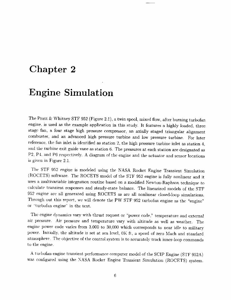
Figure 6.10 shows the response of the internal engine variables (OPR, EPR and N2) due to
the baseline controller inputs (WFPRIB, AREANOZL and VANEHPC). Figure 6.11 shows
normalized measurements, U1MVC, U2MVC, and U3MVC, provided to the baseline con-
troller and the normalized outputs YIMVC, Y2MVC, and Y3MVC. Note that in Figure 6.10
there is excellent tracking of OPR and EPR and as well as tracking of a lagged version of
N2. These responses for the baseline for comparison with the LPV controllers.
Figure 6.12 shows the response of the internal engine variables (OPR, EPR and N2) with
the non-rate bounded LPV controller and Figure 6.13 shows normalized measurements and
outputs of the controller. Note the similarity between the baseline controller commands,
55

Figure 6.10, and the non-rate bounded LPV commands, Figure 6.12. Except for the small
transient that occurs at 1 second due to switching between the baseline controller and the
LPV controller, the engine response is nearly identical. The same excellent tracking of OPR
and EPR and lagged N2 is achieved. It is interesting to see that the normalized controller
YIMVC and Y3MVC commands are very similar. Though for Y3MVC, the baseline con-
troller commands a steady-state value of approximately 12 and the non-rate bounded LPV
controller requests a steady-state value of approximately 2. It appears that this has little
impact on the final N2 speed of the engine.
Figure 6.14 shows the response of the internal engine variables (OPR, EPR and N2) with the
rate bounded LPV controller and Figure 6.15 shows normalized measurements and outputs
of the controller. Note the similarity between the baseline controller commands, Figure 6.10,
the non-rate bounded LPV commands, Figure 6.12, and the rate-bounded LPV commands,
Figure 6.14. The same excellent tracking of OPR and EPR and lagged N2 is achieved. The
non-rate bounded and the rate-bounded LPV controller have very similar control commands,
even the steady-state value of Y3MVC, though the rate-bounded LPV controller has a a low
bandwidth. This can be observed based on the reduced level of high frequency activity
of the normalized control signals U1MVC and U2MVC (see Figures 6.13 and 6.15). The
reduced bandwidth of the rate-bounded LPV controller is exactly what is expected with the
introduction of bounds on the power code rate of variation.
The nonlinear ROCETS simulations with the LPV controllers implemented show that these
controllers are robust to significant changes in the plant dynamics. Recall that the LPV
controllers schedule only on lagged power code and were designed based on linearized engine
models at zero Mach, sea level and standard day atmosphere. The candidate trajectory
starts at sea level Mach 0.4 and reaches a peak altitude of 40,000 ft and speed of Mach
1.2. The performance of the LPV controllers is outstanding despite the large variation in
speed and altitude. The effect of sensor noise on the control algorithms is also of interest.
Therefore, sensor noise is added to the normalized measurements, U1MVC, U2MVC and
U3MVC prior to the controller receiving these signals.
Figures 6.16 and 6.17 show the response of the engine and controller variables with a
small amount (approximately 10%) of sensor noise on control input. The rate bounded LPV
controller is implemented in the ROCETS nonlinear simulation. There is no degradation of
the excellent tracking performance of the controller. Increasing the sensor noise to over 40%,
shown in Figures 6.18 and 6.19 leads to some degradation of the tracking performance though
the overall tracking performance is still adequate. Hence the rate-bounded LPV design is
very insensitive to small amounts of sensor noise as well as changes in the plant dynamics.
For comparison, Figures 6.20 and 6.21 show the response of the baseline controller with over
40% sensor noise. The baseline design is slightly more sensitive to the large amount of sensor
56

noise than the rate-bounded LPV controller.
Similarly, there is no change in the tracking performance of the rate-bounded LPV con-
troller due to temperature fluctuation. Compare the response of the LPV controller on a
standard day, Figures 6.14 and 6.15, with the response on a polar day, Figures 6.22 and 6.23,
and a tropic day, Figures 6.24 and 6.25. Hence, the rate-bounded LPV controller is robust
to significant variations.
The tracking performance of the LPV controller is perhaps better illustrated by holding the
speed constant at zero Mach, standard atmosphere and a constant non-zero altitude. Power
code is varied as a function of time. Figures 6.26 and 6.27 show the response of the non-rate
bounded LPV controller at sea level. This compares well with the rate-bounded LPV design
at sea level, Figures 6.28 and 6.29. Figures 6.30, 6.31, 6.32 and 6.33 show the engine and
rate bounded LPV controller time responses at 15,000 and 30,000 ft altitude respectively. It
is obvious that the engine dynamics change dramatically as a function of altitude.
57

a3 6rr0_4IJ_
_2
00
i i i
10 20 30 40
30
fr 2013_o
10
00
i J i
10 20 30 4O
700
600
o500
_400
3000
i i
10 20 30 40
0(b0--1-I.U -0.2Z<>
6
4fr13_IJJ
2
00
x 104
1.8
1.6v
oJZ 1.4
j_l _ a____ua__(solid)
[ - - request (dash) ]i i J
10 20 30 40
' ' ' 1.210 20 30 40 0
Time (secs)
.._" l - - request (dash) JI
10 20 30 40
Time (secs)
Figure 6,10: Engine response for candidate flight: Baseline Controller
58

0 0.05
_._ ,,, \ _ o_ _2
.7.o.s_ / > -" o '" _jl---'----_ /
0.7 0
;" / I _ _o ' e Co_°x_e_
O_cs ) _o -d_d_te 5_g_t: ]5_se_m
59

___.6rr13_4LL
_2
00
i i i
10 20 30 40
3O
rr 208_0
10
00
* i i
10 20 30 40
700
_.1 600
o_500
_400
3000 10 20 30 40
0(O13_"r"u..I -0.2z<>
-0.4
0 10 20 30 40
Time (secs)
4n"a.UJ
2
v
O4Z 1.4
6
j l__ I- - request (dash)
0 _ '
0 10 20 30 40
x 104
1,8
J"[ - - request (dash) l
1.2, '0 10 20 30 4O
Time (secs)
Figure 6.12: Engine response for candidate flight: Non-Rate Bounded LPV Controller
6O

1.5 0.05
0 1>
>- 0.5
0 10 20 30 40
0>
0
10 20 30 40
0.8 0.02
0.7
>o0.6
>- 0.5
0.40
i i J
10 20 30 40
O> 0.01
o-0.01
-0.020 10 20 30 40
15
010>
e3 5>-
l
0 10 20
Time (secs)
30 40
0>
03
0.05
-0.05 ' '0 10 20 30 40
Time (secs)
Figure 6.13: Controller input and output responses for candidate flight: Non-Rate Bounded
LPV Controller
61

0
20 30 40700
_.1N 600OZ<500ILl
<400
300
10 2O 30 4O
00n2:I.U -0,2
X_o,l0 10
20 30 40Time (secs)
[E
_J
1.8
E 1.6
Z 1.4
1.20 10 20
30
620
010
o 1o2O 30 4O
6 A . -_
0 10 20 "-------'--x 104 30 40
30 40Time (secs)
Figure 6.14: Engine response for candidate flight: Rate Bounded LPV Controller
62

1.5 0.05
O 1>
>- 0.5
00 10 20 30 40
0>
-0.050 10 20 30 40
0.8
0.7
>o0.6
>- 0.5
0.40
i
10 2O 30 4O
0.02
0.01
o>= o
-0.01
-0.020 10 20 30 40
15
(.310>
co 5>-
i i
0 10 20 30 40
Time (secs)
0>
co
0.05
-0.05 ' '0 10 20 30 40
Time (secs)
Figure 6.15: Controller input and output responses for candidate flight: Rate Bounded LPV
Controller
63

8
a3 6EE13-4LL
N2
00
i i
10 20 30 40
3O
n" 2012.0
10
00
_ _solid) 1st (dash)i i i
10 20 30 40
700
Z_600
UJ<500
_400
3000 10 20 30 40
00D."I-LU -0.2Z.<>
-0,4
n-rtUJ
0
1.8
v
04Z 1.4
1.2
0 10 20 30 40
X 104
'_"_" I -- actual (so!id) II - - request (dash) I
i
0 10 20 30 40 0 10 20 30 40
Time (secs) Time (secs)
Figure 6.16: Engine response for candidate flight with small sensor noise: Rate Bounded
LPV Controller
64

1.5
0.05
:1 1o__ ____,o -"o_ J" zu 30 40
0.0." _ r_
o o7_ o O.Ol _._o_ _
-0.01
i
0 10 20 30 40 -0.020 10 20 30
15 _ 40
0.05_ .
010>
o_-- - -
0 _0 20 30 40 -0.05 -- , _
Time (secs) 0 10 20 30 40Time (secs)
Figure 6.17: Controller input and output responses for candidate flight with small sensornoise: Rate Bounded LPV Controller
65

8_
ccn 4I.L
_o_10 20 30 40
,oo/-'-V /
rj 0
;_ -0.2
X-0.4
10 20 30 40
30
n- 20_
Q.0
10
0
0 10 2o 3o 406
Q.UJ
o_10 20 30
x 104 40
1.2Time (secs) 0 10 20 30 40
Time (secs)
Figure 6.18: Engine response for candidate flight with large sensor noise: Rate BoundedLPV Controller
66

1.5
C.) 1>
>- 0.5
0 10 20 30 40
0>
0.051
-0.050 10 20 30 40
0.8
0.7
>o0.6
>- 0.5
0.40
i i i
10 20 30 40
0>
04
0.02
°°'r 1-0.02
0 10 20 30 40
15
010>
5>-
0_--i , i
0 10 20 30
Time (secs)
40
0>
03
0.05
-0.050 10 20 30 40
Time (secs)
Figure 6.19: Controller input and output responses for candidate flight with large sensor
noise: IRate Bounded LPV Controller
67

8
___6n-n4LL
5 2
00 10 20 30 40
3O
n" 20n0
10
00
actual (solid)dash)
i I i
10 20 30 40
7OO
z_600
_500
_400
3000 10 20 30 40
0
_-0.2
-0.4
i i i
0 10 20 30 40
Time (secs)
4rr13_LU
2
1.8
v
Z 1.4
6
/ - - request (dash)0 ' '
0 10 20 30 40
x 104
_' I-- actual !solid)., I._" I - - request (dash) I
1.2 ' ' '0 10 20 30 40
Time (secs)
Figure 6.20: Engine response for candidate flight with large sensor noise: Original Controller
68

1.5 0.05
_ 0>- 0.5 23
0 0 050 0
>- 23
0.40 10 20 30 40 0 10 20 30 40
15
010
_50j-q__
i
0 10 20 30 40 0 10 20 30 40
Time (secs) Time (secs)
O> 0.05_
°23
-0.05
Figure 6.21: Controller input and output responses for candidate flight with large sensor
noise: Original Controller
69

1:136
13_4LJ_
52
00
i i
10 20 30 40
30
rr 2013._O
10
00
A
i i i
10 20 30 40
70O
._1N 600OZ< 500ILlnr"< 400
3000 10 20 30 40
0
o-0.2
>-0.4
i i
0 10 20 30 40
Time (secs)
6
4rr13.IJJ
2
1.8
1.6
O4Z 1.4
1.20
j_[ _ _ctual _olid7
/ - - request (dash) II
0 10 20 30 40
X 10 4
_/ t _ actual (solid) I
_,,,_" , _ _'o requesi (dash) j
10 20 30 4O
Time (secs)
Figure 6.22: Engine response for candidate flight polar day: Rate Bounded LPV Controller
70

1.5 • , 0.05
>- 0.5
0 -0.050 10 20 30 40 0 10 20 30 40
0.8 0.02
0.70
_>0.6
_" 0.5
0.40
i i i
10 20 30 40
0>
0.01
0
-0.01
-0.020
i
10 20 30 40
15
010>
e3 5>-
i i
0 10 20
Time (secs)
0>
co
i
30 40
0.05
-0.050 10 20 30 40
Time (secs)
Figure 6.23: Controller input and output responses for candidate flight polar day: Rate
Bounded LPV Controller
71

8
rn6
00
i 6
10 20 30 40
30
rr 20
0
10
00
_l- _ q ( )J
i i ,
10 20 30 40
7OO
600
500
4003O0
0i i i
10 20 30 40
0L)0."I-UJ -0.2Z<>
rrnUJ
_j - - request (dash) I
0 ' '
0 10 20 30 40
x 104
1.8
o4Z 1.4
-0.4
' ' 1.20 10 20 30 40 0
Time (secs)
/ I
._2" I- li i
10 20 30 40
Time (secs)
Figure 6.24: Engine response for candidate flight tropical day: Rate Bounded LPV Controller
72

1.5 --
(D 1
0._
0.7(.5>
0.6
0.5
10 20 30 40
0.4 fJ
0 10 20 30 40
15,
(..)10>
0
:s03>-
m
ii
10 20 30
Time (secs)40
0.05
0>
0:>
03
O>:m o,f...
-0.050
0.02
10 20 30 40
0.01
0
-0.01
-0.020
0.05 -
10 20 30 4O
-0.05 -- , ,
0 10 20 30 40
Time (secs)
Figure 6.25: Controller input and output responses for candidate flight tropical day: RateBounded LPV Controller
73

m 6
rrQ. 4LL
_2
00
i ,
10 20i
30 40
3O
rr 20nO
10
00
i M i
10 20 30 40
700
._1N 600O
Z500
<1:400
3000
i
10 20i
3O 40
0(J13_"1"uJ -0.2Z
>
V i
crD..uJ
4
2
oo
x lO 4
...-...1.8
E1.6
z 1.4
j__ _ual (solid) l
[ - - request (dash)i J i
10 20 30 40
-0.4
' ' 1.20 10 20 30 40 0
Time (secs)
m
request (dash)i i i
10 20 30 40
Time (secs)
Figure 6.26: Engine response for sea level flight: Non-Rate Bounded LPV Controller
74
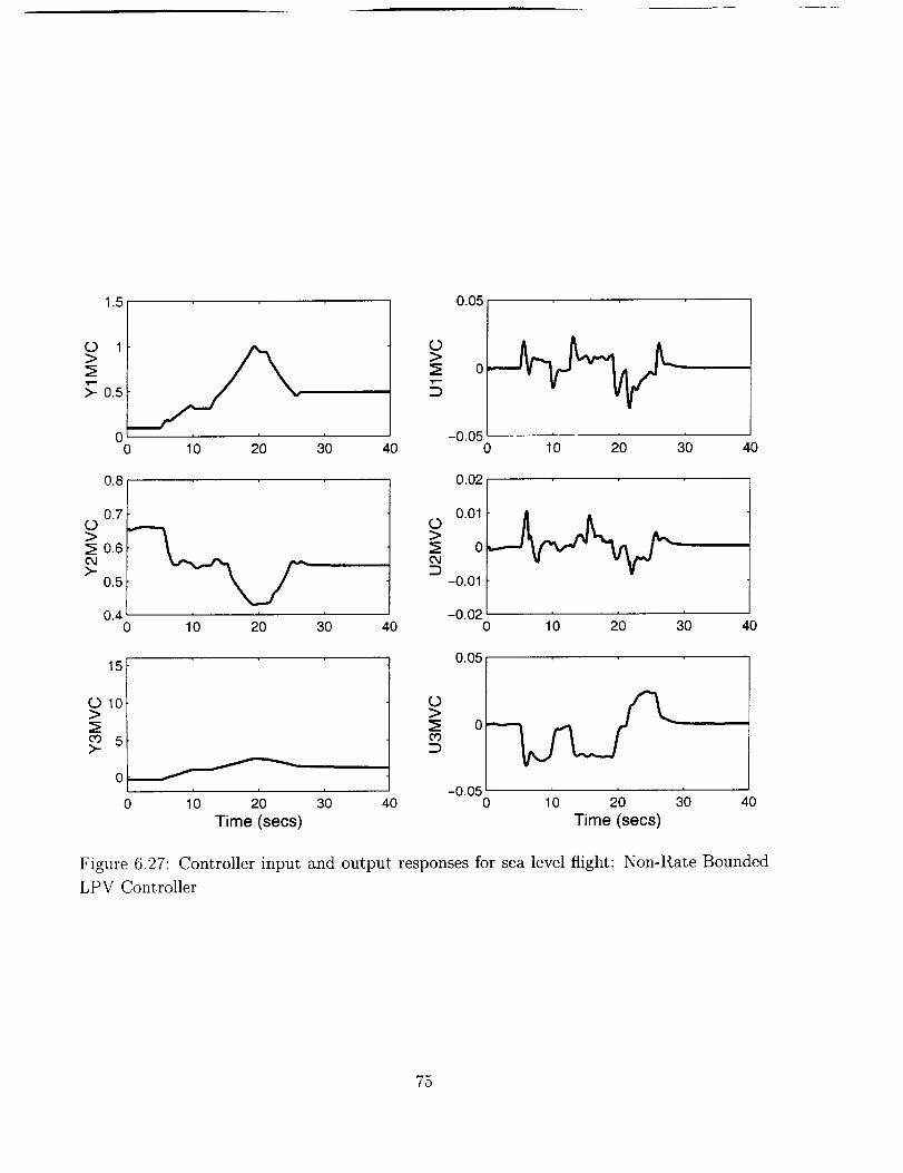
0 10 20 30 40
0.05
0>
-0.050 10 20 30 40
0.8 0.02
0.7O
_>0.6
>" 0.5
0.40
i i
10 20 30 40
O>
0.01
0
-0.01
-0.020
i i
10 20 3O 40
15
O10>
5>-
0>
0.05
' ' -0.050 10 20 30 40 0 10 20 30
Time (secs) Time (secs)
40
Figure 6.27: Controller input and output responses for sea level flight: Non-Rate Bounded
LPV Controller
75

_._6rr0-4i,
52
00
i *
10 20I
3O 4O
30
tr 20
O10
00 10 20 30 40
700
.-IN 600O
_500
_r_'400<
3OO0
i
10 20 3O
0O13_"I-I.U -0.2Z<>
v
4O
rr0_I.U
00
x 104
1.8
E 1.6D..
_1.4
,(solld)
-- request (dash) Ii i
10 20 30 40
' ' 1.210 20 30 40 0
Time (secs)
__/_ req uals(ts(°di::h) I
i * i
10 20 30 40
,Time (secs)
Figure 6.28: Engine response for sea level flight: Rate Bounded LPV Controller
76

1.5 0.05
>- 0.5
00 10 20 30 40
0>
-0.050 10 20 30 40
0.8 0.02
0.7
o>0.6
>" 0.5
0.40
, i
10 20 30 40
0>
0.01
0
-0.01
-0.020
i i
10 20 30 4O
15
010>
eo 5>-
0>
0.05
, ' -0.05 ' ' '0 10 20 30 40 0 10 20 30
Time (secs) Time (secs)
4o
Figure 6.29: Controller input and output responses for sea level flight: Rate Bounded LPV
Controller
77

rn6
rr0_4LL
_2
00
J
10, i
20 30 4O
30
n" 2O0_0
10actual (solid)request (dash) ]
0 10 20 30 40
700
_JN600OZ<500Wn'-<400
3OO0
i
10 20i
30
0-"1"w -0.2Z<>
-0.4
40
EE0-1.11
6
2
0 10
x 104
_ actual (solid) Irequest (dash)i i
20 30 40
1.8
v
04Z 1.4
actual (solid) lrequest (dash) J
' 1.2 '0 10 20 30 40 0 10 20 30 40
Time (secs) Time (secs)
Figure 6.30: Engine response for 15K ff altitude flight: Rate Bounded LPV Controller
78

1.5 0.05
(O 1>
>- 0.5
0
0 20 3010 4O
0>
0
D
10 20 30 40
0.8
0> 0.7_
0.6o,i
>- 0.5
0.40 10 20 30 40
0.02
0 0.01
o04
-0.01
-0.02 ' ' '0 10 20 30 40
15
(DIO>
eo 5>-
0>
¢o
0.05
oJi i i i
0 10 20 30 40 30 40
Time (secs)
-0.05 ' '0 10 20
Time (secs)
Figure 6.31' Controller input and output responses for 15K ft altitude flight: Rate Bounded
LPV Controller
79

rn 6I
rr13.4LL
_2
00
i
10h i
20 30 40
30
rr 200_O
10
00
l I actual (solid)request (dash)i i i
10 20 30 4O
7OO
_JN600OZ<500W13:_:400
3OO0
j-10 20
i
30
0(O13.."1-L.U-0.2Z<>
-0.4
40
4rr13_LU
2
1.8
v
Z 1.4
actual (solid)request (dash) I
0 f i i
0 10 2O 30
10 4
40
actual (solid) ]request (dash) I
' ' ' 12. ' ' '0 10 20 30 40 0 10 20 30 40
Time (secs) Time (secs)
Figure 6.32: Engine response for 30K ft altitude flight: Rate Bounded LPV Controller
8O

1.5 0.05
0 1>
>- 0.5
00 10 20
0>
0
-0.0530 40 0 3010 20 40
0.8
0.70
0.40 10 20 30 40
0.021
0 0.01
°Z3 -0.01
-0,020 10 20 30 40
15
(.310>
5>-
0>
co
0.05
o.... 0.05
0 10 20 30 40 0 10 20
Time (secs) Time (secs)
30 40
Figure 6.33: Controller input and output responses for 30K ft altitude flight: Rate Bounded
LPV Controller
81

Chapter 7
Summary
Recent advances in robust control synthesis for LPV systems were applied to a high fidelity,
nonlinear simulation of a turbofan engine under this research program. The control objective
was to decouple the multivariable system into three independent channels with minimal
cross-coupling, subject to actuator magnitude and rate limitations. 7-/_ point designs
provided an initial starting point, giving an indication of the performance which might be
expected of an LPV controller. After obtaining reasonable point designs, an LPV controller
was synthesized and its performance evaluated.
The nonlinear ROCETS simulation of the Pratt & Whitney engine with the LPV controllers
implemented achieved excellent tracking of the command signals with small magnitude ac-
tuator commands. The rate-bounded LPV controller were robust to significant variations in
the engine model dynamics, atmospheric conditions and sensor noise. Excellent tracking per-
formance was achieved it all scenarios except in the presence of large sensor noise. Although
the synthesis of LPV controllers are computationally more intensive than individual linear
point designs, the guaranteed and actual performance and robustness of the gain-scheduled
LPV designs indicate the benefit of the rate-bounded LPV control designs far out weighs
their computation time expense.
7.1 Acknowledgements
This work was funded by NASA Lewis Research Center, Contract No. NASA/NAG3-1975
with Jonathan Litt as the contract monitor. The authors would like to thank Steve Watts
and Randy Rosson from Pratt &: Whitney and Sanjay Garg from NASA Lewis for help with
the ROCETS code and for insight into the design of multivariable controllers for turbofan
engines.
82

Bibliography
[1] Pratt &: Whitney, CCD 1453-00.0. User's manual for SCIP transient engine simula-
tion. FR-21407B, Aeropropulsion and Power Directorate, Wright Laboratory. Wright-
Patterson AFB, Ohio, Dec. 20, 1996.
[2] D. K. Frederick, S. Garg, and S. Adibhatla. Turbofan engine control design using robust
multivariable control technologies. In AIAA, ASME, SAE, and ASEE Joint Propulsion
Conference, Lake Buena Vista, FL, 1996. AIAA paper _ 96-2587.
[3] A. Packard. Gain scheduling via linear fractional transformations. Systems and Control
Lett., 22(2):79-92, 1994.
[4] A. Packard and M. Kantner. Gain scheduling the LPV way. In Proc. 35th IEEE CDC,
pages 3938-3941, Kobe, Japan, 1996.
[5] G. Becket. Quadratic stability and performance of linear parameter dependent systems.
PhD thesis, University of California, Berkeley, 1993.
[6] F. Wu, A. Packard, and G.J. Balas. LPV control design for pitch-axis missile autopilots.
In Proc. 3_th IEEE CDC, pages 188-193, New Orleans, LA, 1995.
[7] F. Wu, X.H. Yang, A. Packard, G. Becker. Induced L2-norm control for LPV system
with bounded parameter variation rates, in Proc. Amercian Control Conference, pages
2379-2383, Vol. 3, Seattle, WA, 1995.
[8] G. J. Balas, I. J. Fialho, A. K. Packard, J. Renfrow, and C. Mullaney. On the design of
LPV controllers for the F-14 lateral-directional axis during powered approach. In Proc.
1997 ACC, Albuquerque, NM, 1997.
[9] E. Kamen and P. Khargonekar. On the control of linear systems whose coefficients are
functions of parameters. IEEE Trans. Auto. Control, AC-29(1):25-33, 1984.
83

[10]
[11]
[12]
[13]
[14]
[15]
[16]
[17]
[18]
S. M. Shahruz and S. Behtash. Design of controllers for linear parameter-varying systems
by the gain scheduling technique. In Proc. 29th IEEE CDC, pages 2490-2491, Honolulu,
HI, 1990.
J. Shamma and M. Athans. Gain scheduling: potential hazards and possible remedies.
In Proc. 1991 ACC, pages 516-521, Boston, MA, 1991.
P. Apkarian and P. Gahinet. A convex characterization of gain-scheduled H_ controllers.
IEEE Trans. Auto. Control, AC-40(5):853-864, 1995.
G. J. Balas, J. C. Doyle, K. Glover, A. Packard, and R. Smith. #-Analysis and Synthesis
Toolbox (#-Tools). The MathWorks, Inc., Natick, MA, 1991.
A. K. Packard and J. C. Doyle. The complex structured singular value. Automatica,
29(1):71-109, 1993.
G. J. Balas, Jack Ryan, Jong-Yeob Shin, William Garrard. A New Technique for Design
of Controllers for Turbofan Engines. In AIAA, ASME, SAE, and ASEE Joint Propulsion
Conference, Cleveland, OH, 1998. AIAA paper # 98-3751.
K. Zhou, J.C. Doyle, K. Glover. Robust and Optimal Control. Prentice Hall, 1995.
W. Tan, A.K. Packard and G.J. Balas. Quasi-LPV modeling and LPV control of a
generic missile 2000 American Control Conference, Chicago, IL, June, 2000, pp. 3692-
3696.
J.C. Doyle, K. Glover, P.P. Khargonekar, and B.A. Francis. State-space solutions to
standard H2 and H_ control problems. IEEE Trans. Auto. Control, vol. AC-34, no. 8,
August 1989, pp 831-847.
84

Appendix A
User's Guide
A.1 Introduction
This Appendix is intended to be used as a user's manual for the UNIX script files, Matlab
M files, and the modified SCIP transient engine simulations used in this work. The reader
interested in details of the SCIP transient engine simulation is directed to [1].
A.2 Nonlinear Simulation
To simplify the operation of the nonlinear simulation, a series of UNIX script files were
written. They run the correct files and rename the input and output files more descriptively
then the simulation does alone. The file runorig runs the original program provided to the
University or Minnesota. The file runptdes reads in a point-design controller to replace the
Pratt & Whitney controller in the simulation. The file runlpv reads in a LPV controller to
replace the Pratt & Whitney controller. It is assumed in the following discussions that these
script files are being used. These script files are discussed further in Section A.4.
The original and modified versions of the SCIP transient engine simulation read an input file
containing all run parameters, and generate four output files. The input file must end with
the extension ".dat". For example filename, dat is an acceptable name. Three of the output
files are automatically named filename, output, filename, runin, filename, errors. The
name of the fourth output file is chosen by the user in f i lename, dat. The files f ilename, run in,
filename, errors record errors in reading and processing the input file and can be used for
trouble-shooting. The file filename.output, also referred to as the "print file", can be
85

usedto look at specificdata points, and holds any generatedlinear models. The fourth filecontainsthe data suitable for plotting in Matlab. It is often referred to asthe "plot file".
Although the input filesare thoroughly discussedin [1],a quick tutorial is provided on themost relevantaspectsto this work in terms of an examplecontainedin sectionA.3.
The input file is organized in seven blocks of similar function type. The blocks arenamedSCHEDULES, INPUTS, RESTART, OUTPUT, INTEGRATION, EXCEPTIONS,and BALANCE EXCEPTIONS. Eachblock is started with a DEFINE commandandendedwith an END command.
DEFINE (block type)
. . ,
END (block type)
The blocks are read into the simulation in a top-down fashion, so the user must sequence
the blocks accordingly.
A.A.2.1 SCHEDULES
The SCHEDULES block is used to define univariant or bivariant curves representing func-
tional relationships for the model. The curves can be functions of time or steady state point.
The example file defines a schedule called SCHFGR. It is a schedule of thrust (XFCFGR)
with time. The schedule data is listed in standard map reader format; the first two entries
are zero, the third and forth indicate the number of data points of the first and second
independent parameters. The remaining entries are data of the first independent parameter,
the second independent parameter, and the dependent parameter respectively. The example
file's schedule is univariant with time. It has a total of eight data points. Hence the third
entry is "8.0" and the forth is "0.0".
The simulation assumes ramps between each defined point, so a step input can be approx-
imated by placing points close together. In the example, a 200 lbf step is defined at 21.00
seconds. The input power code schedule, along with the output OPR, is plotted in Figure
A.1.
A.A.2.2 INPUTS
The INPUTS block is used to define all inputs to the simulation. The example defines the
altitude (ft), mach number, side slip(degrees), and angle of attack (degrees) to be zero. It
86

definesthe engine face static pressureto be 14.696psi. The thrust is referencedto thescheduledefinedin the precedingSCHEDULESblock as SCHFGR.
A.A.2.3 RESTART
The RESTART block is used to specify a value for the GUESS routine in the simulation.
As in the example file, "0.0" is normally used.
A.A.2.4 1st OUTPUT
The OUTPUT block defines the parameters the simulation is to record in its output files. The
example file tells the simulation to record all the data points of OPR, EPR, N2, OPRREQ,
EPRREQ, N2REQ, and XFCFGR. It instructs the simulation to print them to a file called
test. data.
A.A.2.5 1st RUN
The RUN block provides the simulation with general information on the type of run required.
The first RUN block in the example file tells the simulation to run one point to steady state
using a maximum of of 200 iterations.
A.A.2.6 BALANCE EXCEPTIONS
The BALANCE EXCEPTIONS block is used to turn on or off simulation balances.
A.A.2.7 2nd OUTPUT
The 2nd OUTPUT block in the example file turns off printing to the print file (the . output
file in our case).
A.A.2.8 2nd RUN
The 2nd RUN block in the example file runs a transient simulation and writes the data
requested in the OUTPUT block every 0.05 seconds. It stops the simulation at 30 seconds,
87

no matter what is provided in the SCHEDULE block or elsewherein the input file.
A.A.2.9 Hints
• There is a limit as to how many data points can be plotted in a run. If the simulation
runs, but the plot file has only recorded a single data point, although you instructed
otherwise, try increasing the plot time so you're not asking for as many points.
• While writing input files. Do not use tabs. Only use spaces.
• A * in the first column indicates a comment line
A.3 Example input file
*<DEBUG>
* SClP TRANSIENT ENGINE MODEL (CCD1453-00.0) *
* EXAMPLE FILE *
DEFINE SCHEDULES
,
* THRUST REQUEST T0 ENGINE C0NTROL AS A FUNCTION 0F TIME
SCHEDULE: SCHFGR IS XFCFGK = F(TIME ) ;
SET SCHEDULE: SCHFGR= 0.0, 0.0, 8.0, 0.0,
0.00, 5.00, 9.5, 12.5, 19.00, 21.00,
21.01, 30.0,
27000.0, 27000.0, 27100.0, 27100.0, 26900.0, 26900.0,
27100.0, 27100.0;
END SCHEDULES
* INPUTS *
88

* FLIGHT CONDITION
ALT = 0.0,
XM = 0.0 ,
* FLIGHT CONTROL INTERFACE
XFCFGR = SCHEDULE SCHFGR
XFCAOA = 0.0 ,
XFCBET = 0.0 ,
XFCPO = 14.696 ,
XFCMNL = 0.0 ,
IENGCON = 1
END INPUT
*******************************
* CALL FIRST GUESS ROUTINE *
DEFINE RESTART
GUESS = 0.0;
END RESTART
****************************
* OUTPUT OPTIONS *
****************************
DEFINE OUTPUT
STEADY-STATE PRINT :
TRANSIENT PRINT
PLOT
OFF
OFF
ALL,
ALL,
0PR, EPR, N2,
YIMVC, Y2MVC, Y3MVC,
0PRREQ, EPRREQ, N2REQ,
XFCFGR;
89

PLOTFILE : test.data ;
PLOT TITLE : EXAMPLE FILE DATE;
END OUTPUT
DEFINE RUN
STEADY STATE : POINTS = I., MAXPASS = 200;
END RUN
TURN OFF STEADY STATE ENGINE CONTROL BALANCES *
DEFINE BALANCE EXCEPTIONS
ACTIVATION FOR ANOZLBL2
ACTIVATION FOR WFPRBBL2
ACTIVATION FOR WFABIBL2
ACTIVATION FOR WFAB2BL2
ACTIVATION FOR WFAB3BL2
ACTIVATION FOR VNHPCBL2
ACTIVATION FOR VNFANBL2
ACTIVATION FOR VNECSBL2
ACTIVATION FOR QDOTEHEX
END BALANCE EXCEPTIONS
: OFF ;
: OFF
: OFF
: OFF
: OFF
: OFF
: OFF
: 0FF
: OFF
* TURN OFF PRINT OUTPUT (PLOT OUTPUT IS STILL ON) *
*******************************************************
DEFINE OUTPUT
PRINT : NOPRINT ;
END OUTPUT
* RUN THE TRANSIENT *
DEFINE RUN
TRANSIENT: DT = .0125 , PRINT TIME=5.0, PLOT TIME=O.05,
STOP TIME= 80.00 ;
END RUN
9O

2 715
XFCFQR v$ T_me Ova-all Pressure RalJo vs Time
2 7O5
_ 27
2 695
I
27 05
27
26 95
269
2685
0
268
26 7
2665
2665 10 15 20 25 3_ 5 _0 15 2'3 25
Figure A.I: Power Code and Plant output (P4/P2) from Example File
A.4 UNIX script files and Matlab M files
A.A.4.1 runorig
The script file runorig is used to run the original simulation. After creating an input file as
explained in Section A.2 type
max,. runporig filename
This will run the simulation, creating the four output files.
A.A.4.2 runptdes
The script file runptdes can be used to run a single point controller. Suppose a point design
controller in a # tool system matrix format named sys is to be tested in the nonlinear
91

simulation. The first step is to convert the controller into a Kblock format. This can be
done using the matlab function sys2Kblock.m. The resulting matrix should then be saved
in ascii format to a file named Kblock.
>> Kblock=sys2Kblock(sys,f21);
>> save -ascii Kblock Kblock ;
The next step is to create an input file as described in Section A.2. If the input file is named
filename, dat, the nonlinear simulation can be run by typing
max% runptdes filename
This will run filename.dat using the controller contained in the file Kblock. Note that
runptdes only runs on sun4 architecture, and Kblock must be in the same directory as
test.dat.
A.A.4.3 runlpv
To run a LPV controller scheduled on power code in the nonlinear simulation, the script file
runlpv can be used. The LPV controller must be in a ascii column format as detailed in
the paper, and saved as LPVdata.
>> save -ascii LPVdata Ipv_controller;
All input file, as outlined in Section A.2, can then be run with runlpv. For example, if the
input file is named filename, dat
max_ runlpv filename
Note that LPVdata must be in the same directory as test.dat.
A.A.4.4 data2m.m
Once a nonlinear sinmlation has been run, the data in the plot file can be easily loaded in
matlab with data2m.m. The syntax is
[m,names] =data2m (datafile, flag) ;
92

Here datafile is a string containing the name of the data file. Flag is either "time"or "point". If your simulation was a time responseand savedin filename.data,use thecommand
>> [m,names] =data2m ('filename, data', 'time' );
If your simulation was scheduled as something other than time and saved in f ilename, data,
use the command
>> [m,names] =data2m ('filename, data', 'point ');
The matrix names contains the names of all variable contained in the varying matrix m.
A.A.4.5 engplot.m
Once data from a data file had been loaded into Matlab, it can be plotted with engplot.
For example if the data matrix m contains data for 0PK, you can use the command
>>engplot(m,names,'0PR');
A.5 Plant Linearization
Linear plants can be created by the nonlinear simulation with a LINEARIZATION block in the
input file. As before, I will illustrate usage with an example file. The file can be found in
section A.6
The blocks used for linearization follow the same format as those described above. Two
blocks, LINEARIZATION and LINEAKIZATION EXCEPTIONS define the linearization to be per-
formed. Typically the base point about which linearization is desired, is defined through a
steady state run
DEFINE RUN
STEADY STATE
END RUN
: POINTS = 1., MAXPASS = 200;
93

A.A.5.1 INTEGRATION DEFAULTS and EXCEPTIONS
The states are controlled through the INTEGRATION DEFAULTS and EXCEPTIONS
blocks and the balances through the BALANCE DEFAULTS and EXCEPTIONS blocks.
DEFINE INTEGRATION EXCEPTIONS
ACTIVATION FOR SN2 : STEADY STATE ;
ACTIVATION FOR PTECHD : STEADY STATE ;
ACTIVATION FOR TTECHD : STEADY STATE ;
ACTIVATION FOR SNECS : STEADY STATE ;
ACTIVATION FOR PT65 : STEADY STATE ;
END INTEGRATION EXCEPTIONS
DEFINE BALANCE EXCEPTIONS
ACTIVATION FOR ANOZLBL2 : OFF
ACTIVATION FOR WFPRBBL2 : OFF
ACTIVATION FOR WFABIBL2 : OFF
ACTIVATION FOR WFAB2BL2 : OFF
ACTIVATION FOR WFAB3BL2 : OFF
ACTIVATION FOR VNHPCBL2 : OFF
ACTIVATION FOR VNFANBL2 : OFF
ACTIVATION FOR VNECSBL2 : OFF
ACTIVATION FOR QDOTEHEX : OFF
END BALANCE EXCEPTIONS
A.A.5.2 LINEARIZATION PRINT
The LINEARIZATION PRINT option must be turned on in the OUTPUT block
DEFINE OUTPUT
LINEARIZATION PRINT
END OUTPUT
: ON ;
A.A.5.3 LINEARIZATION
The LINEARIZATION block is used to define the inputs and outputs of the desired linear
model.
94
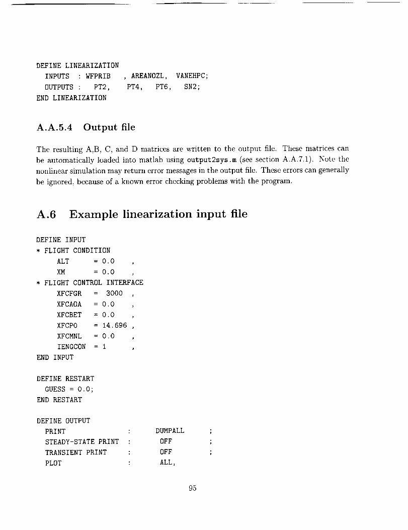
DEFINE LINEARIZATION
INPUTS : WFPRIB , AREANOZL, VANEHPC;
OUTPUTS : PT2, PT4, PT6, SN2;
END LINEARIZATION
A.A.5.4 Output file
The resulting A,B, C, and D matrices are written to the output file. These matrices can
be automatically loaded into matlab using output2sys.m (see section A.A.7.1). Note the
nonlinear simulation may return error messages in the output file. These errors can generally
be ignored, because of a known error checking problems with the program.
A.6 Example linearization input file
DEFINE INPUT
* FLIGHT CONDITION
ALT = 0.0 ,
XM = 0.0 ,
* FLIGHT CONTROL INTERFACE
XFCFGR = 3000 ,
XFCAOA = 0.0 ,
XFCBET = 0.0 ,
XFCPO = 14.696 ,
XFCMNL = 0.0 ,
IENGCON = I
END INPUT
DEFINE RESTART
GUESS = 0.0;
END RESTART
DEFINE OUTPUT
PRINT : DUMPALL
STEADY-STATE PRINT : OFF
TRANSIENT PRINT : OFF
PLOT : ALL,
95

WFPRIB,AREANOZL,VANEHPC,PT2, PT4, PT6, SN2;
PLOTFILE : imp.data ;
PLOT TITLE : LINEARIZE ;
END OUTPUT
DEFINE RUN
STEADY STATE : POINTS = I., MAXPASS = 200;
END RUN
DEFINE INTEGRATION EXCEPTIONS
ACTIVATION FOR SN2
ACTIVATION FOR PTECHD
ACTIVATION FOR TTECHD
ACTIVATION FOR SNECS
ACTIVATION FOR PT65
END INTEGRATION EXCEPTIONS
: STEADY STATE ;
: STEADY STATE ;
: STEADY STATE ;
: STEADY STATE ;
: STEADY STATE ;
* TURN OFF STEADY STATE ENGINE CONTROL BALANCES
DEFINE BALANCE EXCEPTIONS
ACTIVATION FOR ANOZLBL2
ACTIVATION FOR WFPRBBL2
ACTIVATION FOR WFABIBL2
ACTIVATION FOR WFAB2BL2
ACTIVATION FOR WFAB3BL2
ACTIVATION FOR VNHPCBL2
ACTIVATION FOR VNFANBL2
ACTIVATION FOR VNECSBL2
ACTIVATION FOR qDOTEHEX
END BALANCE EXCEPTIONS
: OFF
: OFF
: OFF
: OFF
: OFF
: OFF
: OFF
: OFF
: OFF
DEFINE OUTPUT
LINEARIZATION PRINT : ON
END OUTPUT
DEFINE LINEARIZATION
INPUTS : WFPRIB , AREANOZL, VANEHPC;
96

OUTPUTS : PT2, PT4, PT6, SN2;
END LINEARIZATION
DEFINE LINEARIZATION EXCEPTIONS
NORMALIZER FOR VANEHPC : i00.0 ;
END LINEARIZATION EXCEPTIONS
DEFINE BALANCE EXCEPTIONS
ACTIVATION FOR ANOZLBL2 : OFF ;
ACTIVATION FOR WFPRBBL2 : OFF ;
ACTIVATION FOR VNHPCBL2 : OFF ;
ACTIVATION FOR VNFANBL2 : OFF ;
ACTIVATION FOR VNECSBL2 : OFF ;
ACTIVATION FOR WFABIBL2 : OFF ;
ACTIVATION FOR WFAB2BL2 : OFF ;
ACTIVATION FOR WFAB3BL2 : OFF ;
ACTIVATION FOR QDOTEHEX : ON ;
END BALANCE EXCEPTIONS
DEFINE RUN
LINEARIZE : ;
END RUN
A.7 MORE UNIX SCRIPT and MATLAB files
A.A.7.1 output2sys.m
The Matlab M file output2sys.m reads the linearized plant from the simulation output file
to generate a system matrix. If the output file is named filename, output, for example, the
following command will create a system matrix names sys
>> sys=output2sys ( 'filename ' ) ;
97

A.A.7.2 linearize
The UNIX script file linearize can be used to generate the plant models at 3000, 6000,
9000, ... 30000 lbf thrust by replacing the line
XFCFGR = 3000
in the input file with
XFCFGR = <INSERT_POINT>
The script replaces <INSERT_POINT> with the values listed in the ascii file points generating
a series of linearized plant models.
For example, to create a series of linearized plants at sea level, the INPUT block should have
the form
DEFINE INPUT
* FLIGHT CONDITION
ALT = 0.0 ,
XM = 0.0 ,
* FLIGHT CONTROL INTERFACE
XFCFGR = <INSERT_POINT>
XFCAOA = 0.0 ,
XFCBET = 0.0 ,
XFCPO = 14.696 ,
XFCMNL = 0.0 ,
IENGCON = 1
* IENGCON = 0 ,
END INPUT
The file points is the simple ascii file:
3000.0
6000.0
9000.0
12000.0
15000.0
18000.0
98

21000.0
24000.0
27000.0
30000.0
99

Appendix B
FORTRAN Source Code
This appendix contains the FORTRAN subroutines written for this project. Small explana-
tions are included before each.
B.1 Point Design Implementation
This section contains the FORTRAN code written to implement point design controllers into
the nonlinear simulation.
B.B.I.1 compute_state
The subroutine compute_state is called by the larger simulation. It, in turn, calls all the
other subroutines which read in the controllers and updates the controller states and outputs.
C
Subroutine compute_state(FGRREQ,CRCYBl, CRCYB2, CRCYB3,Ulin,
U2in, U3in, Ylout, Y2out, Y3out)
FORMAL PARAMETERS
REAL Ulin, U2in, U3in
REAL Ylout, Y2out, Y3out
REAL Ylouta, Y2outa, Y3outa
REAL FGRREQ
100

REAL Min(24,1),
REAL P(72,8)
REAL A(24,24)
REAL St(21)
Mout(24,1)
REAL Ylbase, Y2base, Y3base
Integer counter
save St, counter, A
data (St(i), i=1,21)/21_0.0/
data counter /0/
counter=counter+l
if(counter.eq.l) then
CALL GETMXA8(P,72)
Call REFORMMX(P,72,8,A,24,24)
endif
C---MULTIPLY ACROSS THE CONTROLLER
11
Do 11 i=1,21
Min(i,l)=St(i)
Continue
Min(22,1)=Ulin
Min(23,1)=U2in
Min(24,1)=U3in
CALL MULTMX(A,24,24,Min,24,I,Mout,24,1)
22
Do 22 i=1,21
St(i) = Mout(i,l)
Continue
Ylouta = Mout(22,1)
Y2outa = Mout(23,1)
Y3outa = Mout(24,1)
CALL Iinterp(CRCYBI,FGRREQ,Ylbase)
I01

CALL Iinterp(CRCYB2,FGRREQ,Y2base)
CALL Iinterp(CRCYB3,FGRREQ,Y3base)
Ylout = Ylouta + Ylbase
Y2out = Y2outa + Y2base
Y3out = Y3outa + Y3base
RETURN
END
B.B.1.2 linterp
The subroutine linterp is used to linearly interpolate between two points. The vector T
contains x-y data in standard mapping format. A value of x is input as Xin and linterp
returns the corresponding value of y in Yout.
Subroutine linterp(T,Xin,Yout)
C PURPOSE
C Linearly Interpolate between points on a function f(x).
C Given point on f(x), linterp returns f(x) for any value of x.
C
C
C SYNTAX
C CALL linterp(T,Xin,Yout)
C
C T : Data in PW's mapping format (which could be called with tabx2)
C
C Variables passed in:
DIMENSION T(*)
REAL Xin, Your
C Internal Variables:
REAL nx,n
REAL X(IO), Y(IO)
102

INTEGER i
REAL X_high, X_low, Y_high, Y_low
nx = T(3)
Do 500, n=l,nx
X(n)=T(4+n)
Y(n)=T(4+n+nx)
500 CONTINUE
if (Xin.lt.X(1)) then
Yout=Y(2)-(Y(2)-Y(1))/(X(2)-X(1))*(X(2)-Xin)
elseif (Xin.gt.X(nx)) then
Yout=Y(nx-l)+(Y(nx)-Y(nx-l))/(X(nx)-X(nx-l))*(Xin-X(nx-l))
6OO
else
i=l
if (Xin.gt.X(i)) then
i=i+l
go to 600
endif
X_high=X(i)
X_low =X(i-l)
Y_high=Y(i)
Y_low =Y(i-l)
% 2nd: Linerly interpolate the exact value
% the ratio xfcfgr/(pchigh-pclow) = opr/(oprhihg-oprlow)
Yout=(Xin-X_low)/(X_high-X_low)*(Y_high-Y_low) + Y_low
endif
END
103

B.B.1.3 GETMXA8
The subroutine GETMXA8 reads in the controller from a file named Kblock. It inputs the
number of rows to read (r). It returns the matrix read as a r x 8 column matrix A.
SUBROUTINE GETMXA8(A,r)
REAL cl, c2,
Integer r
REAL A(r,8)
INTEGER n
c3, c4, cS, c6, c7, c8
n=O
OPEN (Unit=f5, File='Kblock', STATUS='OLD')
123 READ (15,124,END=125) cl, c2, c3, c4, c5, c6, c7,
124 FORMAT(2X,E14.7,2X,E14.7,2X,E14.7,2X,E14.7,
Pz 2X,E14.7,2X,E14.7,2X,E14.7,2X,E14.7)
n=n+ 1
A(n i) = cl
A(n 2) = c2
A(n 3) = c3
A(n 4) = c4
A(n 5) = c5
A(n 6) = c6
A(n 7) = c7
A(n 8) = c8
GOTO 123
125 n=O
CLOSE (UNIT= 15)
RETURN
END
c8
B.B.1.4 REFORMMX
The subroutine REFORMMXreforms the matrix A (read in by GETMXS) into the correct three
input, three output, 21 state format.
104

SUBROUTINE REFORMMX(A,RI,CI,B,R2,C2)
C THIS SUBROUTINE REFORMS THE 72 by 8 matrix into a 24 by 24
INTEGER RI, R2, CI, C2, BL, R, C, BLOCKS, AR
REAL A(RI,CI)
REAL B(R2,C2)
BLOCKS=RI/R2
4
3
2
Do 2 BL=I,BLOCKS
Do 3 R=I,R2
Do 4 C=I,C1
BC=C+CI* (BL-1)
AR=R+R2*(BL-1)
B(R,BC)=A(AR ,C)
Continue
Continue
Continue
RETURN
END
B.B.1.5 MULTMX
The subroutine MULTMXinputs the matrices A and B along with their dimensions, and returns
the product of A • B in the matrix C.
SUBROUTINE MULTMX(A,AROW,ACOL,B,BROW,BCOL,
C,CROW,CCOL)
THIS SUBROUTINE MULTIPLIES ARRAYS A AND B AND STORES RESULT AS C
INTEGER AROW,ACOL,BROW,BCOL,CROW,CCOL,I,J,K
REAL A(AROW,ACOL),B(BROW,BCOL),C(CROW,CCOL)
LOGICAL ERROR
ERROR= .FALSE.
IF (ACOL.NE.BROW) ERROR = .TRUE.
105

15
25
30
IF (AROW.NE.CROW) ERROR = .TRUE.
IF (BCOL.NE.CCOL) ERROR = .TRUE.
IF (ERROR) THEN
PRINT*, 'ERROR IN THE ARRAY SIZES'
Stop
ELSE
DO 30 I=J,CROW
DO 25 J=I,CCOL
C(I,J) = 0.0
DO 15 K=I,ACOL
C(I,J) = C(I,J) + A(I,K)*B(K,J)
CONTINUE
CONTINUE
CONTINUE
ENDIF
RETURN
END
B.2 Power Code LPV Implementation
B.B.2.1 compute_state
The LPV Implementation, as with the point design code, uses compute_state as it's main
routine and calls all other subroutines from it.
Subroutine compute_state(FGRREQ, CRCYBI, CRCYB2, CRCYB3, Ulin,
& U2in, U3in, Ylout, Y2out, Y3out)
C FORMAL PARAMETERS
REAL Ulin, U2in, U3in
REAL OREQ, EREQ, NREQ
REAL Ylout, Y2out, Y3out
REAL Ylouta, Y2outa, Y3outa
106

REAL FGRREQ
REAL Min(33,1), Mout(33,1)
REAL A(33,33)
REAL St(30)
C YBASE VARIABLES
REAL Ylbase, Y2base, Y3base
save St
data (St(i), i=I,30)/30.0.0/
CALL GETMXA (FGRREQ, A)
C---MULTIPLY ACROSS THE CONTROLLER
ii
Do II i=1,30
Min(i,l)=St(i)
Continue
Min(31,1)=Ulin
Min(32,1)=U2in
Min(33,1)=U3in
CALL MULTMX(A,33,33,Min,33,I,Mout,33,1)
22
Do 22 i=1,30
St(i) = Mout(i,l)
Continue
Ylouta = Mout(31,1)
Y2outa = Mout(32,1)
Y3outa = Mout(33,1)
CALL
CALL
CALL
linterp(CRCYBi,FGRREQ,Yibase)
linterp(CRCYB2,FGRREQ,Y2base)
Iinterp(CRCYB3,FGRREQ,Y3base)
107
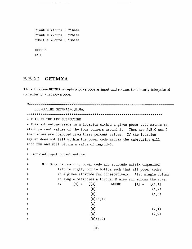
Ylout = Ylouta + YlbaseY2out = Y2outa + Y2baseY3out = Y3outa + Y3base
RETURN
END
B.B.2.2 GETMXA
The subroutine GETMXA accepts a powercode as input and returns the linearly interpolated
controller for that powercode.
Cm ..........
SUBROUTINE GETMXA(PC,BIGA)
THIS IS THE LPV SUBROUTINE
This subroutine reads in a location within a given power code matrix to
*find percent values of the four corners around it. Then new A,B,C and D
*matricies are computed from these percent values. If the location
*given does not fall within the power code matrix the subroutine will
*not run and will return a value of ingrid=0.
* Required input to subroutine:
G - Gigantic matrix, power code and altitude matrix organized
left to right, top to bottom such that all power codes
at a given altitude run consecutively. Also single column
so single matircies A through D also run across the rows.
ex [G] = [ [A] WHERE [A] =
[B]
[C]
[D](i,I)
[A]
[B]
[C]
[D](I,2)
[(1,1)
(1,2)
(1,3)
(2,1)
(2,2)
108

[A]
[B](2,i)
PC - POWER CODE
VEC - power code and iltitude matrix (WAT2)
il - length of PC vector (3,6,9,12,15,18,21,24,27,30) so I0
* Output of subroutine:
*
*
*
*
* Temporary variables:
ingrid - returns 1 if located within WAT2 matrix and
returns 0 if not located within WAT2 matrix and stops
A,B,C,D - new matricies computed from G
* S - temporary matrix not passed through
* alpha.- percent location of WAC2 between points
**********************************************************************
C
integer nr,nc,nx,ny,nu,il,i,j,tl,bl,ii,jj,nt
parameter(il=lO,nx=30,ny=3,nu=3)
real A(30,30),B(30,3),C(3,30),D(3,3)
real alpha,Stmp(IO89),VEC(IO),BIGA(33,33)
real PC, temp
real G(I0890)
Integer counter
C ReadLPV VARIABLES
Integer nxtrue
Real LPVin(10890)
save counter, G
data counter /0/
counter=counter+l
I09

nc=nx+nu
nr=nx+ny*
* Get PC vector
VEC(1)= 3000 0
VEC(2)= 6000 0
VEC(3)= 9000 0
VEC(4)= 12000 0
VEC(5)= 15000 0
VEC(6)= 18000 0
VEC(7)= 21000 0
VEC(8)= 24000.0
VEC(9) = 27000.0
VEC(IO)=30000.O
* Logic function to make temp in bounds
,
temp=PC
if(PC.LT.VEC(1))temp=VEC(1)
if(PC.GT.VEC(il))temp=VEC(il)
,
* P_EAD in G (found through KeadLPV and PadLPV)
,
if(counter.eq.1) then
Call readlpv(nxtrue,LPVin)
Call padLPV(nxtrue,LPVin,G)
endif
* Find contributions of each side and calculate start and end
* point of first matrix (tl=top limet, bl = botom limit)
alpha=O.O
do 20 i=l,il-1
if(temp. GE.VEC(i).AND.temp.LE.VEC(i+l))then
if(temp. NE.VEC(i))then
alpha=(temp-VEC(i))/(VEC(i+1)-VEC(i))
110

end if
tl=nr*nc*(i-l)+l
bl=nr*nc*i
goto 30
end if
20 continue
,
* Compute new A,B,C, and D matricies
,
30 nt=nr*nc
ii=O
do 40 i=tl,bl
ii=ii+l
C
4O
C
50
60
C
70
80
C
Stmp(ii)=G(i)+alpha*(G(i+nt)-G(i))
continue
Make A
ii=O
do 60 i=l,nx
do 50 j=l,nx
ii=ii+l
A(i,j)=Stmp(ii)
continue
continue
Make B
ii=nx*nx
do 80 i=l,nx
do 70 j=l,nu
ii=ii+l
B(i,j)=Stmp(ii)
continue
continue
Make C--
ii=nc*nx
do i00 i=l,ny
do 90 j=l,nx
ii=ii+l
111

90
100
C
110
120
121
122
123
C
124
125
126
C(i, j)=Stmp(ii)
c ont inue
continue
•Make D
ii=nc*nx+nx*ny
do 120 i=l,ny
do II0 j=l,nu
ii=ii+l
D(i, j)=Stmp(ii)
cont inue
continue
.Make it one large matrix .....
do 123 i=l,nx
jj=nx
do 121 j=l,nx
BIGA(i,j)=A(i,j)
continue
do 122 j=l,nu
jj=jj+l
BIGA(i,jj)=B(i,j)
cont inue
continue
ii=nx
do 126 i=l,ny
jj=nx
ii=ii+l
do 124 j=l,nx
BIGA(ii,j)=C(i,j)
continue
do 125 j=l,nu
jj=jj+l
BIGA(ii,jj)=D(i,j)
continue
continue
112

end
B.B.2.3 padLPV
The subroutine padLPV inputs the LPV vector read in by readlpv along with the number
of states of the LPV controller, and returns a LPV vector that has been padded with zeros
so that all controllers have 30 states.
,
C This subroutine rearranges LPVin by moving the zeros
C according to nx. (Largest possible is 30 states, 10 pc vec)
C
Subroutine padLPV(nx,LPVin,LPVout)
Integer nx, i, j, loc, locin, pclength
Real LPVin(10890), LPVout(10890)
C .... A
21
pclength=lO
loc=O
locin=O
Do 99 k=l,pclength
Do 1 i=l,30*(30-nx)
loc=loc+l
LPVout(loc)=O
Continue
Do 2 i=l,nx
Do 21 j=l,30-nx
loc=loc+l
LPVout (loc)=O
Continue
Do 22 j=1,nx
113

22
2
loc=loc+l
locin=locin+l
LPVout(loc)=LPVin(locin)
Continue
Continue
C .... B
Do 3 i=l,3*(30-nx)
loc=loc+l
LPVout(loc)=O
Continue
Do 4 i=l,nx*3
loc=loc+l
locin=locin+1
LPVout(loc)=LPVin(locin)
Continue
C .... C
51
52
5
Do5i=1,3
Do 51 j=l,30-nx
loc=loc+l
LPVout(loc)=O
Continue
Do 52 ]=1,nx
loc=loc+1
locin=locin+l
LPVout(loc)=LPVin(locin)
Continue
Continue
C .... D
Do 6 i=I,9
loc=loc+l
locin=locin+l
LPVout (loc) =LPVin (loc in)
114

6 Continue
99 Continue
End
END subroutine
B.B.2.4 readLPV
The subroutine readlpv reads in the LPV vecctor from an external file named LPVdata and
returns it along with the number of states contained in each of the vectors controllers. It
assumes there are a total of 10 controllers in the LPV vector.
C
C This subroutine reads in the LPV controller from LPVdata
C It must be called before compute_state b/c it provides the
C number of states to be used in compute_state
C (Assumes PCvec length of I0, Max number of states=30)
C
9
10
11
Subroutine readlpv(nxi,LPV)
Integer num, nxi, counter
Real LPV(I0890), LPVlocal(10890),
save counter, LPVlocal, nx
nx
data counter /0/
counter=counter+l
if(counter.eq.l) then
num=O
OPEN (Unit=19, File='LPVdata', STATUS='OLD')
num=num+ 1
READ(19,10,end=11) LPVlocal(num)
FORMAT(2X,FI4.7)
go to 9
CLOSE(UNIT=Ig)
115

endif
nx=sqrt(real(num/lO))-3
nxi=int(nx)
12
do 12 i=l,num
LPV(i)=LPVlocal(i)
continue
END
C END subroutine
The LPV implementation also calls the subroutines linterp and mutlmx which are listed
in the Point Design section above.
B.3 Compilation
The full engine simulation consists of three FORTRAN files and an assortment of auxiliary
files containing common data blocks. The main files are
ccd1453_eng_con.f
ccd1453..main.f
ccd1453_roc_util.f
ccd1453_eng_mod.f
ccd1453_roc_.run.f
The auxiliary files need are
CLCASCOM
CLCCOM
ECSCASCOM
ECSCCOM
NCCCOM
NCCOM
NCSCOM
SHKCCOM
116

To compilethe programwith a new control algorithm copy in into ccd1453_eng_con,f. Forexample, if the new control algorithm was in a file namednewcontrol, f, type
cp newcontrol.f ccd1453_eng_con.f
Then run the makefile on a sun4 architecture by typing
Y_ax make
This runs the UNIX script file Makefile. sun4. It was written to compile, and link all the
components.
117

Appendix C
Line by Line Example
This Appendix lists the specific commands to run a ROCETS simulation using
• The PW simulation
• A point design simulation
• A LPV simulation
Note that this Appendix is strictly intended for those working in Dr. Gary Balas' lab who
have access to the Sun machines max and/or marlowe. At this point, the ROCETS simula-
tions only run on sun4 architecture. The example files are located at/home/res6/j ackryan/pwfl/Examp
These directions are also located at/home/res6/j ackryan/pwfl/Examples/HowToRun, txt.
Before running the following examples, type the line
_ax set path=(/home/res6/jackryan/Script /home/res6/jackryan/pwfl/PwScripts $path)
It adds the path which contains all the necessary UNIX script files. Also add the paths
>>
>>
>>
path('/home/res6/jackryan/pwfl/m',path);
path('/home/res6/jackryan/pwfl/m/MakeModel',path);
path('/home/res6/jackryan/pwfl/m/TestModel',path);
in Matlab. The}' contain all the necessay Matlab M files.
118

C.1 The original Pratt & Whitney simulation
To run the original Pratt & Whitney simulation, go to the directory/home/res6/j ackryan/pwfl/Exampl
and type
maxZ pwd
/home/res6/jackryan/pwfl/Examples
maxZ runorig example
Running example (sun4 version) ..
max%
It creates the files
example.errors
example.runin
example.output
fort.25
test.data
: Contains any error messages if any occurred
: a filtered copy of example.dat which is
sent to the program. Lists .dat file errors
the end (good for trouble shooting)
: values of a single point in the run
: a link to example.dat
: The plot file. Lists all the data of the run.
Now load and plot the data into Matlab by typing the commands at a Matlab prompt
>> [m,names]=data2m('test.data','time');
First line of data: i0
Number of data points: 722
Heading variables:
TIME EPR EPRREQ FGR N2 N2REQ
OPR OPRREQ WAC2 XFCFGR XFCFGR YIMVC
Y2MVC Y3MVC
Number of variables found: 14
>> engplot(m,names,'EPR','EPRREQ');
The variable EPK is is ambiguous.
Using the first occurrence of EPR
>> print -deps epr_plotl
>>
119

C.2 Running a Point Design
Now run the Point Design version. The file Kblock contains a point designed controller.
The controller must be in a file named Kblock. First move test. data to test. orig. data
so that the PW simulation results are not over-written.
max_ mv test.data test.lpv.data
max_ runptdes example
Running example (sun4 version)
maxZ
In Matlab, load and plot the new data
>> opr_plot(m,mp,names,'EPR');
The variable EPR is is ambiguous.
Using the first occurrence of EPR
The variable EPR is is ambiguous.
Using the first occurrence of EPR
>> print -deps epr_plot2
>>
C.3 Running a LPV Design
Now run the LPV version. LPVdata contains the LPV controller; the program looks for
LPVdata so the controller must have this name. First move test. data to test. orig. data
so the results from the point design simulation will not be over-written
max_ mv test.data test.orig.data
maxZ runlpv example
Running example (sun4 version) ..
max_
In Matlab, load the new data and plot the new and old together
>> [ml,names]=data2m('test.data','time');
First line of data: i0
120

Number of data points: 722
Reading variables:
TIME EPR EPRREQ FGR N2 N2REQ
OPR OPRREQ WAC2 XFCFGR XFCFGR YIMVC
Y2MVC Y3MVC
Number of variables found: 14
>> opr_plot(m,ml,names,'EPR');
The variable EPR is is ambiguous.
Using the first occurence of EPR
The variable EPR is is ambiguous.
Using the first occurrence of EPR
>> print -deps epr_plot3
>>
All files used and created in these examples are contained in/home/res6/j ackryan/pwfl/Examples/.
There are a few more executables (alllocatedin/home/res6/j ackryan/pwfl/PwScripts/)
which have not been specifically mentioned. They are run in the same fashion as listed above.
They are
runorig Runs the original ROCETS
runptdes Run a point design controller
runlpv Run an LPV controller scheduled on power code
runlpvl Run an LPV controller scheduled on lagged power code
runtemp Used to run temporary codes for testing (I just use it
for ease ... it's not necessary)
All the FORTRAN source code used in this project is located at
/home/res6/jackryan/pwfl/src/
The various control algorithm source code files are listed and described below
121

Ipv_lag. f
jack_ml_eng_con.lpv.f
jack_ml_eng_con.lpv2d.f
jack_ml_eng_con.ptdes.f
wac2.1ag.lpv.new.f
wac2.1pv.new.f
LPV code which schedules on lagged PC
(run with runlpvl)
LPV code scheduled on PC
(run with runlpv)
LPV code scheduled on 2 variables
(In a proof of concept stage)
Point Design code (reads in Kblock)
(run with runptdes)
LPV code scheduled on filtered WAC2
(run with runwacl)
LPV code scheduled on WAC2
(run with runwac)
122