ARGONNE NATIONAL LABORATORY9700 South Cass Avenue

Lemont, IL 60439

Nonlinear Robust Optimization

Sven Leyffer, Matt Menickelly, Todd Munson, Charlie Vanaret, and Stefan M. Wild

Mathematics and Computer Science Division

Preprint ANL/MCS-P9040-0218

January 31, 2018

This material was based upon work supported by the U.S. Department of Energy, Office of Science, Office of Advanced Scientific

Computing Research, under Contract DE-AC02-06CH11357.

Updates to this preprint may be found at http://www.mcs.anl.gov/publications

Contents

1 Introduction and Notation 1

2 Nonlinear Robust Optimization Formulations and Theory 22.1 The Nominal Problem . . . . . . . . . . . . . . . . . . . . . . . . . . . . . . . . . . . . 32.2 Stationarity Conditions for Nonlinear Robust Optimization . . . . . . . . . . . . . . 32.3 Stationarity Conditions for Problem with Implementation Errors . . . . . . . . . . . 52.4 Distributionally Robust Optimization . . . . . . . . . . . . . . . . . . . . . . . . . . . 6

3 Applications and Illustrative Examples 83.1 Applications of Nonlinear Robust Optimization . . . . . . . . . . . . . . . . . . . . . 83.2 Illustrative Examples . . . . . . . . . . . . . . . . . . . . . . . . . . . . . . . . . . . . . 9

4 Solution Approaches 104.1 Bilevel Approach to Robust Optimization . . . . . . . . . . . . . . . . . . . . . . . . . 104.2 Reformulations of Classes of Robust Optimization Problems . . . . . . . . . . . . . . 114.3 Methods of Outer Approximations . . . . . . . . . . . . . . . . . . . . . . . . . . . . . 154.4 Algorithms for Robust Optimization with Implementation Errors . . . . . . . . . . . 16

5 Software for Robust Optimization 17

6 Nonconvexity and Global Optimization 18

7 Conclusion 20

ii

Nonlinear Robust Optimization

Sven Leyffera, Matt Menickellya, Todd Munsona, Charlie Vanareta, and Stefan M. Wilda

aMathematics and Computer Science Division, Argonne National Laboratory, 9700 South Cass Ave.,Argonne, IL 60439, USA

ARTICLE HISTORY

Compiled February 7, 2018

ABSTRACTRobust optimization (RO) has attracted much attention from the optimization community over thepast decade. RO is dedicated to solving optimization problems subject to uncertainty: design con-straints must be satisfied for all the values of the uncertain parameters within a given uncertaintyset. Uncertainty sets may be modeled as deterministic sets (boxes, polyhedra, ellipsoids), in whichcase the RO problem may be reformulated via worst-case analysis, or as families of distributions. Thechallenge of RO is to reformulate or approximate robust constraints so that the uncertain optimiza-tion problem is transformed into a tractable deterministic optimization problem. Most reformulationmethods assume linearity of the robust constraints or uncertainty sets of favorable shape, which rep-resents only a fraction of real-world applications. This survey addresses nonlinear RO and includesproblem formulations and applications, solution approaches, and available software with code sam-ples.

Keywords: Nonlinear robust optimization.

AMS-MSC2000: 90C30, 62K25.

1. Introduction and Notation

Over the past decade, robust optimization has attracted much attention. A number of excellentsurveys and monographs exist [10,17,22,38,44,60], which deal mainly with linear and conic cases.Related papers on the general class of semi-infinite optimization can also be found, for example,in [47,66–68,70]. This survey focuses on nonlinear robust optimization (NRO), which is becomingmore important in real-world applications. The NRO problem is

minimizex∈X

f(x)

subject to c(x;u) ≤ 0, ∀u ∈ U(x),(1.1)

where x ∈ Rn are the decision variables, X ⊆ Rn is the certain feasible set, u ∈ Rp are the uncer-tain parameters, U(x) is the uncertainty set, and the constraints c(x;u) model the impact of the

Preprint ANL/MCS-P9040-0218CONTACT: Sven Leyffer. Email: leyffer@anl.gov

Nonlinear Robust Optimization 2

uncertainty on the design. Formally, we define U(x) : Rn → Rp as a set-valued mapping repre-senting the uncertainty set with c : Rn+p → Rq the robustness criteria. Whenever the uncertaintyset U(x) is of infinite cardinality, the problem (1.1) is a semi-infinite nonlinear optimization prob-lem. We assume throughout that all functions are smooth on the appropriate sets. We can relaxthis assumption for some algorithms, provided we are prepared to deal with subgradients. Wealso assume that U(x) is a nonempty, compact set for all x ∈ X . If U(x) were empty for all x ∈ X ,then the uncertainty constraint could be removed. The compactness assumption ensures that theuncertainty is bounded (unbounded uncertainty is not typically encountered in real-world appli-cations). If the uncertainty set u ∈ U is independent of the decision variables x and the constraintsare separable in x and u, c(x;u) = g(x) + d(u) ≤ 0, then we can replace the uncertain constraintby a deterministic constraint, provided that we can (globally) solve

d∗ := maxu∈U

d(u),

where the max is computed separately for each component of d(u). In this case, the uncertaintyconstraint becomes c(x;u) = g(x) + d∗ ≤ 0.

We can accommodate minimax problems in robust optimization, where the objective functiondepends on uncertain parameters, in the formulation (1.1) by introducing an additional variablefor the epigraph of the uncertain objective, thereby moving the uncertain objective to c(x;u). Wenote that, without loss of generality, we can assume that U(x) = U1(x) × · · · × Uq(x) and that theuncertain constraints can be written as cj(x;u) ≤ 0, ∀u ∈ Uj(x); see [17]. Thus, we can treat eachrobustness constraint individually. For ease of presentation, however, we limit our discussionhere to the single constraint case (q = 1), although the methods target problems with multipleconstraints.

In the remainder of this paper, we provide background for robust optimization and differentformulations in Section 2, applications and example problems in Section 3, an overview of so-lution approaches in Section 4, a description of available software in Section 5, a discussion ofnonconvexity and global optimization in Section 6, and conclusions in Section 7.

Notation. Throughout the survey, we use the convention that finite sets are denoted by romanletters and infinite sets by calligraphic letters. The decision variables are denoted by x ∈ Rn,and the uncertain parameters are denoted by u ∈ Rp. The (deterministic) set of feasible points isdenoted by X , and the set of uncertain parameters is denoted by U . We denote the nominal valueof the uncertain parameters by u ∈ U . In many applications, the nominal value, u, is the value ofthe parameters that the system would take in the absence on uncertainty.

2. Nonlinear Robust Optimization Formulations and Theory

Here we discuss a number of important special cases of nonlinear robust optimization. We startwith a description of the nominal optimization problem and its properties and provide station-arity conditions for the standard robust optimization formulation. We then consider minimaxproblems that arise when we need to handle implementation errors, before discussing a special

Nonlinear Robust Optimization 3

form of robust optimization, called distributionally robust optimization.

2.1. The Nominal Problem

In general, we can derive a relaxation of the nonlinear robust optimization problems, (1.1), byenforcing the robust constraints over a subset of uncertain parameters. Of particular interest is afinite subset, U ⊂ U , which results in a nonlinear optimization relaxation. The (global) solution toany such relaxation yields a lower bound. The nominal problem is a particular relaxation obtainedby choosing U = u and is defined as

minimizex∈X

f(x)

subject to c(x; u) ≤ 0,(2.2)

which is a finite-dimensional nonlinear problem. We make the following observations:

(1) It follows that the nominal problem is a relaxation of (1.1), which implies that its (global)solution provides a lower bound on the solution of (1.1).

(2) Clearly, if the feasible set x | c(x; u) ≤ 0, is empty, then it follows that (2.2), and hence(1.1), has no solution.

(3) However, if (2.2) has no solution, then it does not follow that the robust problem (1.1) hasno solution, as illustrated by the following example showing that robustness can immunizea problem against unbounded solutions.

Consider the two-dimensional problem

minimizex∈R2

x1 + x2 subject to u1x1 + u2x2 − u21 − u22 ≤ 0, ∀u ∈ [−1, 1]2,

which corresponds to minimizing x1 + x2 inside the unit ball. Setting the nominal value ofthe uncertain parameters as u = (

√32 ,

12), it follows that the nominal problem is unbounded

(Figure 1a), while the robust problem has an optimal solution at x = (− 1√2,− 1√

2) (Figure 1b).

2.2. Stationarity Conditions for Nonlinear Robust Optimization

First-order optimality conditions for (1.1) have been derived by John; see, for example, [47, 68].We start by defining the active index set for the active constraints,

U0(x∗) := u ∈ U | c(x∗;u) = 0 .

Theorem 2.1 (Stationarity Conditions for Robust Optimization [47,68]). Let x∗ be a local minimizerof (1.1) (and X = Rn). Then there exist a finite subset U ′0(x

∗) ⊂ U0(x∗) and multipliers λi ≥ 0 for eachu(i) ∈ U ′0(x∗) such that

λ0∇f(x∗) +∑

u(i)∈U ′0(x∗)

λi∇xc(x∗;u(i)) = 0, λ0 +∑

u(i)∈U ′0(x∗)

λi = 2. (2.3)

Nonlinear Robust Optimization 4

−2 2

−2

2

−1 1

−1

1

√3

2x1 + 1

2x2 = 1

x1 + x2 = k

x1

x2

(a) Unbounded nominal problem

−2 2

−2

2

−1 1

−1

1x1 + x2 = −√2

x1

x2

(b) Bounded NRO

Figure 1.: Unbounded nominal problem and bounded NRO.

We note, that the constant “2” in the multiplier sum can be replaced by any positive number, butour choice simplifies the derivation of stationarity conditions for problems with implementationerrors in Section 2.3.

We say that x∗ is a stationary point of (1.1) if x∗ satisfies (2.3). We note that for λ0 = 0, theseconditions are related to the stationarity conditions of the robust nonlinear feasibility problem

minimizex

maxu∈U(x)

12

∥∥c(x;u)∥∥22.

Moreover, if x∗ satisfies an extended constraint qualification, we can replace the Fritz-Johncondition in Theorem 2.1 with the Karush-Kuhn-Tucker condition [47]

∇f(x∗) +∑

u(i)∈U ′0(x∗)

λi∇xc(x∗;u(i)) = 0

with λi ≥ 0 for each u(i) ∈ U ′0(x∗).The stationarity condition (2.3) is not as useful as standard Fritz-John conditions in nonlin-

ear optimization because the index set U0(x∗) can contain an infinite number of points and hasno closed-form characterization. Moreover, even given U0(x∗), one still needs to find u(i) and λi

simultaneously to satisfy (2.3), which in general is a set of nonlinear equations.We can show that x∗ is a stationary point of (1.1) if and only if dx = 0 solves a linearized robust

optimization problem:

Theorem 2.2. A robust feasible point, x∗, is a stationary point of (1.1) if, and only if, dx = 0 solves thefollowing linearized problem:

minimizedx

∇f(x∗)Tdx

subject to c(x∗;u) +∇xc(x∗;u)Tdx ≤ 0, ∀u ∈ U(x)

x∗ + dx ∈ X .(2.4)

Nonlinear Robust Optimization 5

Proof. We start by stating the stationarity conditions of (2.4) at dx = 0. If dx = 0 solves (2.4), thenit follows again by Theorem 2.1 that there exist a finite subset U ′′ ⊂ U(x∗) and multipliers νi ≥ 0

for all u(i) ∈ U ′′ such that

ν0∇f(x∗) +∑

u(i)∈U ′′νi∇xc(x∗;u(i)) = 0, ν0 +

∑u(i)∈U ′0

νi = 2, (2.5)

holds.Next, we show that if x∗ is a stationary point of (1.1), then dx = 0 solves (2.4). If x∗ is stationary,

then it follows that c(x∗;u) ≤ 0, ∀u ∈ U(x), which implies that dx = 0 is feasible in (2.4). To seethat dx is also a stationary point, we simply compare the stationarity conditions (2.5) and (2.3).

Finally, we show that if dx solves (2.4), then x∗ is a stationary point of (1.1). The equivalence ofthe first-order conditions can be seen by comparing (2.5) and (2.3), and feasibility of x∗ followsfrom the feasibility of dx = 0:

c(x∗;u) +∇xc(x∗;u)Tdx ≤ 0, ∀u ∈ U(x) ⇒ c(x∗;u) ≤ 0, ∀u ∈ U(x),

which concludes the proof.

It may seem surprising that Theorem 2.2 does not require any constraint qualification or condi-tions on U(x) to hold. However, these conditions are implicitly assumed in the stationarity of x∗,which implies the existence of multipliers.

To the best of our knowledge, the stationarity condition of Theorem 2.2 is new. However, wenote that unless U(x), c(x∗;u), and ∇xc(x∗;u) have special structure, the linearized robust opti-mization problem (2.4) is not necessarily easier to solve than (1.1), because it is still a nonlinearproblem in u. We observe that if U(x) = U is independent of x and polyhedral or conic, then(2.4) is a tractable linear or conic optimization problem; see Section 4.2. A simpler stationaritycondition is obtained if we consider the active constraints, replacing u ∈ U by u ∈ U0(x∗) or evenu ∈ U ′0(x∗) in (2.4).

2.3. Stationarity Conditions for Problem with Implementation Errors

In many applications, we are interested in decision variables x that are robust to manufacturingerrors or general implementation errors. Problems of this kind can be expressed as a minimaxoptimization problem

minimizex∈X

maxu∈U(x)

f(x+ u), (2.6)

which could be expressed equivalently in the form of (1.1) as

minimizex∈X ,t∈R

t

subject to f(x+ u)− t ≤ 0, ∀u ∈ U(x).(2.7)

Nonlinear Robust Optimization 6

We note that U = U(x) may depend on the decision variables x; but in the existing literature thatexplicitly considers (2.6), this is not the case.

A characterization of robust local minima, as well as descent directions at a point x, for theminimax function given in (2.6) can be found in [20]. The work in [20] considers the special casewhere X = Rn and U = u | ‖u‖2 ≤ ∆ for some ∆ > 0, because this particular uncertainty setallows for easily stated sufficient conditions for a point in Rn to be a robust local minimum of(2.6). For general U(x), we can describe necessary conditions for a point x being a robust localminimum by using the conditions of Theorem 2.1 applied to (2.7); these conditions in this case areequivalent to the existence of λi ≥ 0 such that∑

u(i)∈U ′0(x∗)

λi∇f(x∗ + u(i)) = 0∑u(i)∈U ′0(x∗)

λi = 1.(2.8)

One can show that these necessary conditions are in fact equivalent to the sufficient conditionsderived in [20] given their particular choice of U .

Observing that in (2.8), the set U ′0(x∗) is equivalent to the set

argmaxu∈U(x∗)

f(x∗ + u),

there is a natural geometric interpretation of these conditions, which we illustrate in Figure 2given X = R2 and U = u | ‖u‖2 ≤ ∆. In Figure 2b, we have |U ′0(x∗)| = 3, and the correspondinggradients ∇f(x∗ + u(i)) positively span R2. Hence, the necessary (and in this case, sufficient)conditions in (2.8) are satisfied. In Figure 2c, we have |U ′0(x∗)| = 1 (and u(1) occurs in the interiorof U(x∗)); because ∇f(x∗ + u(1)) = 0, the conditions in (2.8) are also satisfied in this case. Theexample in Figure 2c also illustrates how for nonconvex f , the concept of a robust local mimimumcan be practically dissatisfying, as there is an open neighborhood about x∗ so that every point inthe neighborhood is also a robust local minimum for (2.6).

In Figure 2a, we observe that given∇f(x+u(1)) and∇f(x+u(2)), there do not exist nonnegativemultipliers such that (2.8) can be satisfied, implying that x cannot be a robust local minimum. Al-though we will not go into the algebraic details here, Figure 2a also illustrates the related conceptof a cone of descent directions for (2.6) at a point x. It is geometrically intuitive that the shadedarea of Figure 2a is a cone of descent, since for any small perturbation s such that x + s is in thecone, neither x+ u(1) nor x+ u(2) will be in U(x+ s). Thus, the maximum value of the inner prob-lem of (2.6) given U(x+ s) is strictly bounded above by the maximum value of the inner problemof (2.6) given U(x), implying that s is a descent direction.

2.4. Distributionally Robust Optimization

A topic of increasing interest in the past decade has been distributionally robust stochastic op-timization (DRSO). The typical problem of stochastic optimization, without any reformulations,

Nonlinear Robust Optimization 7

x+ u(1) x+ u(2)

3634

32

30

28

28

26

26

24

24

22

22 20

20

20

18

18

18

16

16

16

16

16

14

14

14

14

14

12

12

12

12

12

10

10

1010

10

8

8

8

8

8

66

6

4

4

4

2

2

−2 −1 0 1 2−2

−1

0

1

2

x

(a)

x∗ + u(1)

x∗ + u(2) x∗ + u(3)

9.59.5 99

8.58.5

88

7.5

7.5

7.5

7.5

7

7

7

7

77 7 7 7 7 7

6.5

6.5

6.5

6.5

6.5

6.5

6.56.5 6.5 6.5 6.5 6.5 6.5

6

6

6

6

6

6

66 6 6 6 6 6

5.5

5.5

5.5

5.5

5.5

5.5

5.5

5.5

5.55.5 5.5 5.5 5.5 5.5 5.5

5

5

5

5

55

5

5

5

55 5 5 5 5 5

4.5

4.5

4.5

4.5

4.5

4.5

4.5

4.5

4.5

4.54.5 4.5 4.5 4.5 4.5 4.5

4

4

4

4

4

4

4

4

44 4 4 4 4 4

3.5

3.5

3.5

3.5

3.5

3.5

3.5

3.5

3.53.5 3.5 3.5 3.5 3.53.5

3

3

3

3

3

3

3

3

333 3 3 3

3

2.52.52.5

2.5

2.5

2.5

2.52.5

2.5

2.5

2.52.5

2

2

2

222

2

2

2 2

1.51.51.5

1.5

1.5

1.5

1.5

1

1

1

1

1

0.5

0.5

0.5

0

−1 0 1 2−2

−1

0

1

x∗

(b)

0.4

0.3

0.3

0.2

0.2

0.2

0.1

0.1

0.1

0.1

0.10

0−0.1

−0.1

−0.1

−0.1

−0.1

−0.2

−0.2

−0.2

−0.3

−0.3−

0.4

−1.5 −1 −0.5 0 0.5 1 1.5−2

−1

0

1

2

x∗

x∗ + u(1)

(c)

Figure 2.: Geometric intuition for (a) descent directions of (2.6) at a point x, (b),(c) x being a robustlocal minimum of (2.6)

can be cast as an unconstrained problem

minimizex∈X

Eπ[f(x, π(ω))

], (2.9)

where E is the expectation operator, π : Ω → Rd is a measurable probability distribution, Ω is asample space, and the objective function is a mapping f : X × Rd → R. Generally, however, amodeler does not have access to a closed-form distribution π, and it is thus desirable to considera robust version of (2.9)

minimizex∈X

maxπ∈P

Eπ[f(x, π(ω))

], (2.10)

introducing an uncertainty set P of possible distributions. As in (2.7), the minimax problem in(2.10) can be reformulated as a problem of the form (1.1).

Much of the existing research in DRSO focuses on developing uncertainty sets P so that thesolution of (2.10) is tractable. A dominant strategy [16, 28] considers first- and second-order mo-

Nonlinear Robust Optimization 8

ments µ and Σ of empirically observed realizations of π(ω) and P is defined as a set of probabilitydistributions having first- and second-order moments “close” to µ and Σ. A more recent, butpromising, strategy [32, 65] assumes that some reference nominal distribution π is known, andthen defines P as the set of distributions “close” to π in a measure-theoretic sense, the so-calledWasserstein distance. We will not discuss either of these strategies in any further detail, but wepoint to the cited papers and the references therein.

We remark on a direction of research that is also referred to as distributionally robust optimiza-tion but is notably different from the one presented in (2.10), which led to the development ofthe ROME software package [40, 41]. That body of work is concerned with nominal linear opti-mization problems and the tractable reformulations of robustified linear constraints. In [40, 41],uncertainty sets may be constructed to leverage knowledge of distributional properties of theuncertainty such as bounds on moments, bounds on the distributional support, and directionaldeviations. The work in [40, 41] is also extended to compute nonanticipative (but relatively sim-ple) decision rules for multistage problems while maintaining tractability.

3. Applications and Illustrative Examples

Here we provide examples of nonlinear robust optimization problems considered in the literature.We emphasize cases with infinite-cardinality uncertainty sets, but we note that finite-cardinalityuncertainty set examples are prevalent; see, for example, the minimax regret and test problemsin [33,45,46]. The illustrative examples in Section 3.2 are used in later sections to demonstrate thesolution techniques and available software.

3.1. Applications of Nonlinear Robust Optimization

Robust convex quadratically constrained optimization problems have been solved for applica-tions including financial portfolio selection problems [43], equalization of time-invariant commu-nication channels [62], and statistical learning problems [42, 49].

Designing truss and frame structures under uncertain loads [8] and design of antenna arrays[14] have also been addressed from a nonlinear optimization perspective.

A number of control problems involving uncertain initial and state conditions result in nonlin-ear robust optimization problems. Spacecraft attitude control was addressed through a minimaxapproach in [25] and the scheduling of industrial processes was the subject of [54]. The chemi-cal engineering problem of batch distillation was considered by using an elliptic uncertainty setin [29, 30].

Robust optimization has also been considered in situations where the objective function oruncertain constraints are available only through the output of a simulation. Examples of theseinclude the design of a DC–DC converter [26] and electromagnetic matching for nanophotonicengineering [19, 20].

Nonlinear Robust Optimization 9

3.2. Illustrative Examples

We use the following examples throughout the paper to illustrate our approaches. These problemsall have objective functions that are smooth on the appropriate sets and have nonempty, compactuncertainty sets. In addition, they satisfy the following conditions:

C1 The certain feasible set X is convex and f(x) is a convex function.C2 The uncertainty set U(x) is convex and compact for all x.C3 The robust constraints c(x;u) ≤ 0 are convex in x and concave in u.

We discuss the implications if some of the convexity assumptions are relaxed in Section 6.Our first example is a simple two-dimensional problem in which the uncertainty set is inde-

pendent of the variables, x.

Example 3.1. Consider the following robust optimization problem illustrated in Figure 3.minimize

x≥0(x1 − 4)2 + (x2 − 1)2

subject to x1√u− x2u ≤ 2, ∀u ∈

[14 , 2] (3.11)

•

0 2 4 6 8 100

2

4

6

8

10

x1

x2

Figure 3.: The two-dimensional robust optimization problem from Example 3.1

Our second example is built from a 3-SAT problem, and exemplifies the situation when theuncertainty set also depends on th variables, x.

Example 3.2. Consider the following special case of a robust 3-SAT problem [61],minimize

x∈X−x1

subject to x1 − u1x5 − u2x6 ≤ 0, ∀u ∈ U(x),(3.12)

Nonlinear Robust Optimization 10

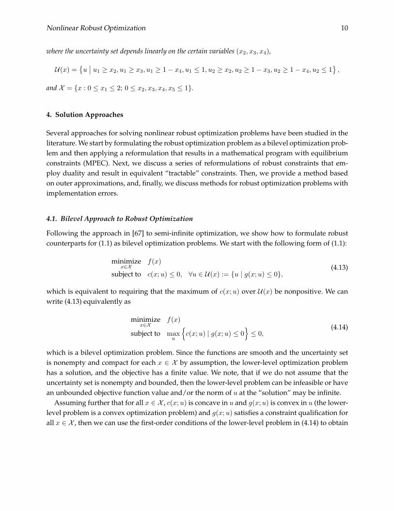
where the uncertainty set depends linearly on the certain variables (x2, x3, x4),

U(x) =u∣∣ u1 ≥ x2, u1 ≥ x3, u1 ≥ 1− x4, u1 ≤ 1, u2 ≥ x2, u2 ≥ 1− x3, u2 ≥ 1− x4, u2 ≤ 1

,

and X = x : 0 ≤ x1 ≤ 2; 0 ≤ x2, x3, x4, x5 ≤ 1.

4. Solution Approaches

Several approaches for solving nonlinear robust optimization problems have been studied in theliterature. We start by formulating the robust optimization problem as a bilevel optimization prob-lem and then applying a reformulation that results in a mathematical program with equilibriumconstraints (MPEC). Next, we discuss a series of reformulations of robust constraints that em-ploy duality and result in equivalent “tractable” constraints. Then, we provide a method basedon outer approximations, and, finally, we discuss methods for robust optimization problems withimplementation errors.

4.1. Bilevel Approach to Robust Optimization

Following the approach in [67] to semi-infinite optimization, we show how to formulate robustcounterparts for (1.1) as bilevel optimization problems. We start with the following form of (1.1):

minimizex∈X

f(x)

subject to c(x;u) ≤ 0, ∀u ∈ U(x) := u | g(x;u) ≤ 0,(4.13)

which is equivalent to requiring that the maximum of c(x;u) over U(x) be nonpositive. We canwrite (4.13) equivalently as

minimizex∈X

f(x)

subject to maxu

c(x;u) | g(x;u) ≤ 0

≤ 0,

(4.14)

which is a bilevel optimization problem. Since the functions are smooth and the uncertainty setis nonempty and compact for each x ∈ X by assumption, the lower-level optimization problemhas a solution, and the objective has a finite value. We note, that if we do not assume that theuncertainty set is nonempty and bounded, then the lower-level problem can be infeasible or havean unbounded objective function value and/or the norm of u at the “solution” may be infinite.

Assuming further that for all x ∈ X , c(x;u) is concave in u and g(x;u) is convex in u (the lower-level problem is a convex optimization problem) and g(x;u) satisfies a constraint qualification forall x ∈ X , then we can use the first-order conditions of the lower-level problem in (4.14) to obtain

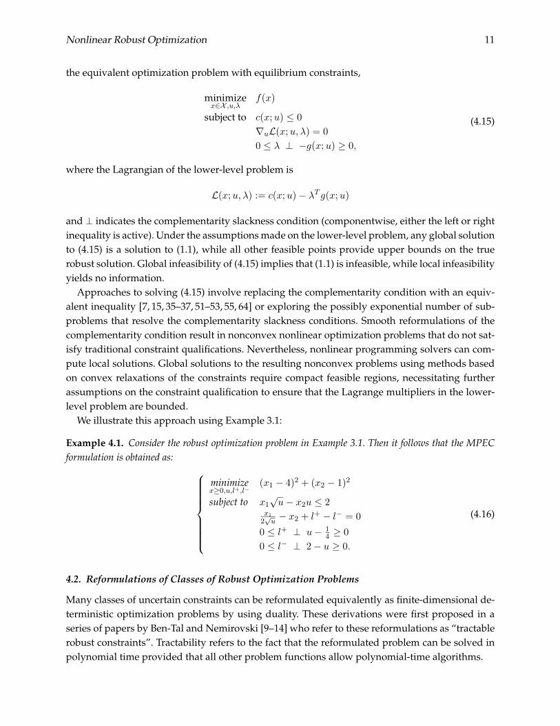
Nonlinear Robust Optimization 11

the equivalent optimization problem with equilibrium constraints,

minimizex∈X ,u,λ

f(x)

subject to c(x;u) ≤ 0

∇uL(x;u, λ) = 0

0 ≤ λ ⊥ −g(x;u) ≥ 0,

(4.15)

where the Lagrangian of the lower-level problem is

L(x;u, λ) := c(x;u)− λT g(x;u)

and ⊥ indicates the complementarity slackness condition (componentwise, either the left or rightinequality is active). Under the assumptions made on the lower-level problem, any global solutionto (4.15) is a solution to (1.1), while all other feasible points provide upper bounds on the truerobust solution. Global infeasibility of (4.15) implies that (1.1) is infeasible, while local infeasibilityyields no information.

Approaches to solving (4.15) involve replacing the complementarity condition with an equiv-alent inequality [7, 15, 35–37, 51–53, 55, 64] or exploring the possibly exponential number of sub-problems that resolve the complementarity slackness conditions. Smooth reformulations of thecomplementarity condition result in nonconvex nonlinear optimization problems that do not sat-isfy traditional constraint qualifications. Nevertheless, nonlinear programming solvers can com-pute local solutions. Global solutions to the resulting nonconvex problems using methods basedon convex relaxations of the constraints require compact feasible regions, necessitating furtherassumptions on the constraint qualification to ensure that the Lagrange multipliers in the lower-level problem are bounded.

We illustrate this approach using Example 3.1:

Example 4.1. Consider the robust optimization problem in Example 3.1. Then it follows that the MPECformulation is obtained as:

minimizex≥0,u,l+,l−

(x1 − 4)2 + (x2 − 1)2

subject to x1√u− x2u ≤ 2

x1

2√u− x2 + l+ − l− = 0

0 ≤ l+ ⊥ u− 14 ≥ 0

0 ≤ l− ⊥ 2− u ≥ 0.

(4.16)

4.2. Reformulations of Classes of Robust Optimization Problems

Many classes of uncertain constraints can be reformulated equivalently as finite-dimensional de-terministic optimization problems by using duality. These derivations were first proposed in aseries of papers by Ben-Tal and Nemirovski [9–14] who refer to these reformulations as “tractablerobust constraints”. Tractability refers to the fact that the reformulated problem can be solved inpolynomial time provided that all other problem functions allow polynomial-time algorithms.

Nonlinear Robust Optimization 12

As in Section 4.1, the derivation starts from (4.14), and we assume that for all x ∈ X , c(x;u)

is concave in u and g(x;u) is convex in u and that g(x;u) satisfies a constraint qualification forall x ∈ X . Rather than writing the first-order conditions of the lower-level problem, we insteadform its dual, such as the Lagrangian or Fenchel dual. In particular, robust counterparts of non-linear uncertain constraints for general convex functions can be found by exploiting the supportfunction δ∗ and the concave conjugate function c∗ [9]. The authors show that

c(x;u) ≤ 0, ∀u ∈ U := u | Du+ q ≥ 0

if and only if

x, v satisfy δ∗(v | U)− c∗(x; v) ≤ 0.

This result allows general convex sets. In general, however, no closed-form expressions exist ei-ther for the conjugate of a convex function or for the support function. [9, Table 3] lists expressionsfor conjugates of some simple functions. We illustrate this approach with the Wolfe dual, and ar-rive at the problem

minimizex∈X

f(x)

subject to minu,λ

L(x;u, λ) | ∇uL(x;u, λ) = 0, λ ≥ 0

≤ 0,

(4.17)

where the Lagrangian of the lower-level problem is

L(x;u, λ) := c(x;u)− λT g(x;u)

and λ ≥ 0 are the Lagrange multipliers of the lower-level constraints. We can now omit the in-ner minimization because if we find any (u, λ) such that L(x;u, λ) ≤ 0, then it follows that theminimum is nonpositive. Thus, we arrive at the single-level problem

minimizex∈X ,u,λ

f(x)

subject to L(x;u, λ) ≤ 0

∇uL(x;u, λ) = 0

λ ≥ 0.

(4.18)

For nonlinear functions, the resulting problem is typically a nonconvex optimization problem.Under the assumptions made on the lower-level problem, any global solution to (4.18) is a solu-tion to (1.1), while all other feasible points provide upper bounds on the true robust solution. If(4.18) is globally infeasible and there is no duality gap, then (1.1) is also infeasible. If either thereis a duality gap or (4.18) is only locally infeasible, then we cannot draw any conclusions. We notethat for some nonconvex problems, one can also show that the duality gap is zero, see, e.g. [24].

A connection exists between (4.18) and (4.15). We observe that both have the condition that∇uL = 0 and λ ≥ 0. Adding λT g(x;u), which equals zero from the complementarity slackness

Nonlinear Robust Optimization 13

condition, to c(x;u) shows that (4.18) is a relaxation of (4.15). The difference, however, is theconclusions that can be drawn when these two problems are globally infeasible.

We illustrate the Wolfe-dual approach using Example 3.1.

Example 4.2. Consider the robust optimization problem in Example 3.1. Then it follows that the Wolfe-dual formulation is given by

minimizex≥0,u,l+≥0,l−≥0

(x1 − 4)2 + (x2 − 1)2

subject to x1√u− x2u− 2 + l+(u− 1

4) + l−(2− u) ≤ 0x1

2√u− x2 + l+ − l− = 0,

(4.19)

Our general form (4.18) recovers the robust counterpart of a linear robust constraint.

Example 4.3. Consider the following problem:

minimizex∈X

f(x)

subject to (a+ Pu)T x ≤ b, ∀u ∈ U := u | Du+ q ≥ 0,(4.20)

where P,D are matrices of suitable dimensions such that U is compact. We see that (4.20) becomes

minimizex∈X ,u

f(x)

subject to maxu

(a+ Pu)T x− b | Du+ q ≥ 0

≤ 0,

which is equivalent to the Wolfe-dual problem

minimizex∈X ,u,λ

f(x)

subject to minu,λ

(a+ Pu)Tx− b+ λT (Du+ q) | P Tx+DTλ = 0, λ ≥ 0

≤ 0.

Exploiting the fact that P Tx+DTλ = 0, we arrive at the following tractable formulation:

minimizex∈X ,λ

f(x)

subject to aTx+ λT q ≤ bP Tx+DTλ = 0, λ ≥ 0,

whose constraints are a (finitely generated) polyhedral set. This approach has been generalized to otherforms of polyhedral constraints that we summarize in Table 1.

Unfortunately, these reformulations often result in significantly more-complex constraints, asillustrated by the following example.

Example 4.4. Robust convex quadratic optimization problems of the form

minimizex∈Rn

cTx | 1

2xTQx+ xT g + γ ≤ 0, ∀(Q, g, γ) ∈ U

(4.21)

Nonlinear Robust Optimization 14

were first reformulated as equivalent semidefinite programming (SDP) problems in [11]. Problems of thisform can also be cast as equivalent second-order cone programming (SOCP) problems. For example, [42]show that for polytopic and factorable uncertainty sets, as well as affine uncertainty sets of the form

U =

(Q, g, γ) | Q = Q0 +

p∑i=1

λiQi, (g, γ) = (g0, γ0) +

p∑i=1

vi(gi, γi),

‖λ‖ ≤ 1, ‖v‖ ≤ 1, Qi 0, ∀i,

(4.22)

one obtains an equivalent SOCP formulation for (4.21).

Classes of Tractable Robust Constraints. An overview of tractable robust constraints is found inTable 1. The reformulations depend on the specific form of the uncertain constraint c(x;u) andthe specific form of the uncertainty set U . These reformulations may be computationally moreexpensive than other approaches [18]. A more detailed form of Table 1 can be found in Tables 1and 2 of [9], which provide classes of tractable reformulations for uncertainty sets and problemfunctions, respectively.

Table 1.: Reformulations of robust constraints.

Uncertain Constraint Uncertainty Set Tractable Constraint Ref.

Affine Polyhedral Polyhedral [11](a+ Pu)T x ≤ b Du+ q ≥ 0 aTx+ qTλ ≤ b

P Tx+DTλ = 0, λ ≥ 0

Affine `∞-Box Polyhedral [11](a+ Pu)T x ≤ b ‖u‖∞ ≤ ρ aTx+ ρ‖P Tx‖1 ≤ bAffine `2-Ball Conic constraint [11](a+ Pu)T x ≤ b ‖u‖2 ≤ ρ aTx+ ρ‖P Tx‖2 ≤ bAffine Closed convex pointed cone K Conic constraint [13](a+ Pu)T x ≤ b Du+ q ∈ K aTx+ qTλ ≤ b

P Tx+DTλ = 0, λ ∈ K∗Convex quadratic Convex set, u ∈ C Semidefinite constraint [58]xTA(u)x+ b(u)Tx+ c ≤ 0 A(u) = A+ U, b(u) = b+ Ub

Conic quadratic Convex set, u ∈ C Semidefinite constraint [58]√xTA(u)x+ b(u)Tx+ c ≤ 0 A(u) = A+ U, b(u) = b+ Ub

Convex quadratic Ellipsoid SDP [11]Conic QP Ellipsoid SDP [11]SDP Structured ellipsoid SDP [11]Convex function Convex set Conjugate convex [9]

Classes of Intractable Robust Constraints. Classes of robust-constraint and uncertainty-set com-

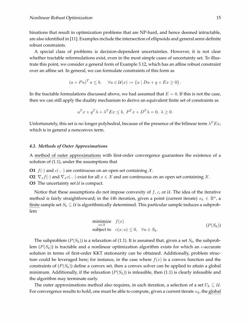
Nonlinear Robust Optimization 15

binations that result in optimization problems that are NP-hard, and hence deemed intractable,are also identified in [11]. Examples include the intersection of ellipsoids and general semi-definiterobust constraints.

A special class of problems is decision-dependent uncertainties. However, it is not clearwhether tractable reformulations exist, even in the most simple cases of uncertainty set. To illus-trate this point, we consider a general form of Example 3.12, which has an affine robust constraintover an affine set. In general, we can formulate constraints of this form as

(a+ Pu)T a ≤ b, ∀u ∈ U(x) := u | Du+ q + Ex ≥ 0 .

In the tractable formulations discussed above, we had assumed that E = 0. If this is not the case,then we can still apply the duality mechanism to derive an equivalent finite set of constraints as

aTx+ qTλ+ λTEx ≤ b, P Tx+DTλ = 0, λ ≥ 0.

Unfortunately, this set is no longer polyhedral, because of the presence of the bilinear term λTEx,which is in general a nonconvex term.

4.3. Methods of Outer Approximations

A method of outer approximations with first-order convergence guarantees the existence of asolution of (1.1), under the assumptions that

O1 f(·) and c(·, ·) are continuous on an open set containing X .O2 ∇xf(·) and ∇xc(·, ·) exist for all x ∈ X and are continuous on an open set containing X .O3 The uncertainty set U is compact.

Notice that these assumptions do not impose convexity of f , c, or U . The idea of the iterativemethod is fairly straightforward; in the kth iteration, given a point (current iterate) xk ∈ Rn, afinite sample set Sk ⊆ U is algorithmically determined. This particular sample induces a subprob-lem

minimizex∈X

f(x)

subject to c(x;u) ≤ 0, ∀u ∈ Sk.(P (Sk))

The subproblem (P (Sk)) is a relaxation of (1.1). It is assumed that, given a set Sk, the subprob-lem (P (Sk)) is tractable and a nonlinear optimization algorithm exists for which an ε-accuratesolution in terms of first-order KKT stationarity can be obtained. Additionally, problem struc-ture could be leveraged here; for instance, in the case where f(x) is a convex function and theconstraints of (P (Sk)) define a convex set, then a convex solver can be applied to attain a globalminimum. Additionally, if the relaxation (P (Sk)) is infeasible, then (1.1) is clearly infeasible andthe algorithm may terminate early.

The outer approximations method also requires, in each iteration, a selection of a set Uk ⊆ U .For convergence results to hold, one must be able to compute, given a current iterate xk, the global

Nonlinear Robust Optimization 16

maximum to max c(xk;u) : u ∈ Uk. For problems where c(xk;u) is concave in u for all u ∈ U ,then selecting Uk = U for all k may not be unreasonable. Similarly, if one knows from particularproblem structure that c(xk;u) is concave on a subset U ′k ⊂ U , then one might select Uk = U ′k andsolve the maximization problem to global optimality. In general, however, if global optimalitycannot be guaranteed, such as in the case of (2.6) where f is nonconvex, then one may use finitesets Uk ⊂ U . For convergence in the general case, however, one needs to ensure that Uk → U ,namely, that some form of asymptotic density holds.

A statement of an inexact method of outer approximations is given in Algorithm 1.

Choose initial point x1 ∈ Rn.Choose a sequence εk → 0 such that εk > 0 for all k, and set k ← 0.Choose s0 ∈ U .for k = 0, 1, 2, . . . do

Choose a finite set Sk satisfying s0, . . . , sk ⊂ Sk.Let xk be an εk-accurate solution to (P (Sk)).Choose Uk ⊂ U .Let sk be a global maximizer of arg max

u∈Uk

c(xk;u).

k ← k + 1.end

Algorithm 1: Method of Outer Approximations.

It has been proved (e.g., in Chapter 3.5 of [63]), that every accumulation point of Algorithm 1applied to (1.1), under a rigorous version of the previously stated assumptions, satisfies a first-order stationary condition.

4.4. Algorithms for Robust Optimization with Implementation Errors

An algorithm for solving NROs with implementation errors is proposed in [20]. The algorithmiteratively solves a sequence of second-order conic optimization subproblems intending to finddescent directions as in Figure 2a. The algorithm assumes access only to an oracle capable offunction and gradient evaluations of f . Provided f is convex and continuously differentiable, theauthors show that the proposed algorithm converges to the global optimum of (2.6). This methodis augmented by a simulated annealing method in [19] in an attempt to offer asymptotic globalguarantees for nonconvex problems.

The black-box algorithm in [27] considers (2.6) when only function evaluations (i.e., no gra-dient evaluations) of f are available. The algorithm in that work alternates between obtainingapproximate local minima and maxima to the outer and inner problems of (2.6), respectively, viasmooth model-based trust-region optimization methods. No convergence guarantees on the pro-posed method are made. A recent unpublished work [59] considers (2.6) again under black-boxassumptions. The algorithm in that work is based on a method of outer approximations, as inSection 4, and solves a sequence of nonsmooth optimization problems over local surrogate mod-els. The iterates of the algorithm are shown to cluster at Clarke stationary points of the minimax

Nonlinear Robust Optimization 17

function of (2.6), a condition that is directly related to the robust local minima of [20] but for moregeneral U(x). The convergence result in [59] does not assume f to be convex.

A recently published work [69] handles (2.6) with (optional) additional robust constraints ofthe form

c(x+ u) ≤ 0 ∀u ∈ U . (4.23)

The method targets more general robust optimization problems and proposes building separatemetamodels of the objective in (2.6) and the constraints in (4.23) via kriging. Solving these surro-gate problems is then passed to a (relatively) inexpensive global optimization operation.

5. Software for Robust Optimization

Modeling languages for robust optimization serve as an intermediate layer between the mod-eler and numerical solvers. Such languages usually implement several strategies for instantiatingan uncertain problem into a tractable certain problem. We list here relevant major modeling lan-guages.

• AIMMS [23] is an integrated combination of a modeling language, a graphical user interface,and numerical solvers. It supports deterministic robust optimization and distributionallyrobust optimization (the model includes chance constraints whose probability is associatedwith the specific distribution).• JuMPeR [1] is an algebraic modeling toolbox for robust and adaptive optimization in Julia.

It extends the syntax of JuMP. Its resolution techniques include cutting planes.• ROC [21] is a C++ software package for formulating and solving distributionally adaptive

optimization models.• ROME [40, 41] (Robust Optimization Made Easy) is an algebraic modeling toolbox in Mat-

lab. It implements distributionally robust optimization (parameterized by classical proper-ties, such as moments, support, and directional deviations) and robust decision-making, inwhich the uncertainties are progressively revealed.• ROPI [39] is a C++ library for solving robust mixed-integer linear problems modeled in the

MPS file format.• SIPAMPL [70] is an environment that interfaces AMPL with a semi-infinite programming

solver. Uncertain parameters (or infinite variables) are represented by names starting witht, and constraints that involve uncertain parameters are represented by names starting witht (see Listing 1 for the code for Example 3.1).

Listing 1: SIPAMPL modelvar x 1..2 >= 0; # decision variables

var t; # uncertain parameter

minimize fx: (x[1] - 4)ˆ2 + (x[2] - 1)ˆ2; # deterministic objective

Nonlinear Robust Optimization 18

subject to

tcons: x[1]*sqrt(t) - x[2]*t <= 2; # robust constraint

bounds: 0.25 <= t <= 2; # uncertainty set

• YALMIP [56, 57] is a free Matlab toolbox, developed initially to model SDP problems andsolve them by interfacing external solvers. It was later extended to deterministic robust opti-mization (see Listing 2) and distributionally robust optimization. YALMIP implements sev-eral strategies (called filters) for instantiating an uncertain problem into a tractable certainproblem, including duality, enumeration, explicit maximization, conservative approxima-tion, and elimination.

Listing 2: YALMIP modelsdpvar x1 x2 t % decision variables

constraints = [x1*sqrt(t) - x2*t <= 2, % robust constraint

x1 >= 0, x2 >= 0,

0.25 <= t <= 2, % uncertainty set

uncertain(t)]; % uncertain parameter

objective = (x1 - 4)ˆ2 + (x2 - 1)ˆ2; % deterministic objective

solvesdp(constraints, objective)

Table 2, inspired by [31], compares their features. To the best of our knowledge, no model-ing language supports generalized semi-infinite optimization, including the case when we havedecision-dependent uncertainty sets that depend on x.

Table 2.: Robust optimization modeling toolboxes.

Solver Language Open Solvers Uncertainty Sets Constraints Examples

AIMMS AIMMS 7 Many box, ellipsoidal, convex linear [6]JuMPeR Julia 3 Many polyhedral, ellipsoidal, custom linear [2]ROC C++ 3 CPLEX polyhedral, ellipsoidal linearROME Matlab 3 SDPT3, polyhedral, ellipsoidal linear [3]

MOSEK,CPLEX

ROPI C++ 3 CPLEX, finite set of scenarios linearGurobi,Xpress

SIPAMPL AMPL/Matlab 3 NSIPS box nonlinear [4]YALMIP Matlab 3 Many polyhedral, ellipsoidal, linear, quadratic, 2nd order, [5]

conic semidefinite cone

6. Nonconvexity and Global Optimization

We are interested in investigating the challenges involved in extending the work surveyed inthe preceding sections to nonconvex robust optimization. We consider only nonconvexities in the

Nonlinear Robust Optimization 19

robust constraint and the uncertainty set, namely,

c(x;u) ≤ 0, ∀u ∈ U := u | g(u) ≤ 0.

We are interested in the tractability of this set of constraints.The best-case situation arises when Assumptions C2 and C3 from Section 3.2 are satisfied. Un-

der these assumptions, the problems arising in the sampling/outer approximations approach areconvex minimization and concave maximization problems. Moreover, the duality gap is zero, andwe can apply the reformulations of the MPEC section. Table 3 summarizes how this situation de-teriorates if we relax the assumptions on c(x;u). In general, the problems marked as nonconvexin Table 3 require global optimization techniques such as branch and bound, making them signi-ficantly harder than the best-case.

Table 3.: Properties of problems in Polak’s outer approximation approach under different convex-ity assumptions, assuming that U is convex.

Property of c(x;u) Sampling Outerx-convex u-concave Problem Approx.

3 3 concave max. convex min.3 7 nonconvex convex min.7 3 concave max. nonconvex7 7 nonconvex nonconvex

We note that nonconvexity/nonconcavity in x/u requires convex/concave under-/over-estimators to be built that are parameterized in u/x, respectively, as the following example il-lustrates.

Example 6.1. Consider the following robust constraint,

c(x;u) := x2 − x21u ≤ 0, ∀u ∈[

1

2,3

2

],

and assume that X = [0, 1]2. Then it follows that we can build secant relaxations for every u as

c(x;u) := x2 − x1u ≤ 0, ∀u ∈[

1

2,3

2

].

However, the situation becomes harder if the class of underestimator depends on the value of u. For example,for U = [−1

2 ,12 ], it follows that c(x;u) is convex in x for u ≤ 0, and we need only the underestimator for

u ≥ 0.

Table 3 also shows that the situation is more difficult for robust optimization problems thatinvolve implementation errors, because c(x;u) = c(x + u) is convex in x and concave in u if andonly if it is affine.

Nonlinear Robust Optimization 20

We turn now to the case of nonconvex uncertainty sets U . In this case, only the separable andpartially linear case is easy, because

c(x;u) := c1(x) + bTu ≤ 0, ∀u ∈ U ⇔ c1(x) + maxu∈U

bTu ≤ 0.

Now, observe that a linear function attains its maximum at an extreme point of the feasible set, sowe can equivalently maximize over the convex hull of U , namely,

c(x;u) := c1(x) + bTu ≤ 0, ∀u ∈ U ⇔ c1(x) + maxu∈conv(U)

bTu ≤ 0.

Of course, finding the convex hull conv(U) is not trivial. Even worse, this simple trick alreadyfails if we relax the linearity in u to concavity in u, namely, for c(x;u) := c1(x) + c2(u) with c2(u)

concave, because the maximum of a concave function no longer occurs at an extreme point, andreplacing U by its convex hull will overestimate the uncertainty set and result in a conservativeestimate.

7. Conclusion

Overall, nonlinear robust optimization problems, while naturally occurring and apparently ofpractical importance - see our discussion of various practical applications, implementation er-rors, and distributionally robust optimization - have not yet matured to the state of conic robustoptimization problems. This maturity level is not surprising when viewed through the lens ofreformulation. As we have discussed, affine constraints coupled with uncertainty sets of favor-able shape lead to linear or conic optimization problems and are hence deemed tractable from theperspective of convergence rates to global optimality, whereas something as seemingly innocu-ous as decision-dependent uncertainty may lead to NP-hard reformulations. As the state of theart continues to improve for nonconvex (nonsmooth) optimization, more problems may becometractable in practice via solutions to MPEC reformulations of bilevel problems or applications ofouter approximation methods.

The literature on nonlinear robust optimization is expanding and encompasses areas we did notconsider in this survey. In some applications, we have the opportunity to take corrective actionafter (part of) the uncertainty is revealed. Robust optimization problems with this sort of struc-ture fall into the class of two-stage decision problems [40, 41], where the decision variables x arefirst-stage, or here-and-now, decisions, and a second set of variables y(u) represents wait-and-see,second-stage, or recourse decisions. Robust optimization is connected to robust model-predictivecontrol [29, 30, 48, 50]. These are problems where the decision variables are time-dependent stateand control variables that are governed by a system of differential algebraic equations that de-scribe the dynamics of the underlying physical system. Robust optimization problems can alsoinclude integer decision variables [34].

To summarize, much opportunity exists for growth and novel research in the field of nonlinearrobust optimization, driven by relevance and practical application, which will also spur further

Nonlinear Robust Optimization 21

developments in general nonconvex (and NP-hard) optimization.

Acknowledgments

This material is based upon work supported by the U.S. Department of Energy, Office of Science,Office of Advanced Scientific Computing Research, under Contract DE-AC02-06CH11357.

References

[1] JuMPeR: algebraic modeling for robust and adaptive optimization. https://github.

com/IainNZ/JuMPeR.jl.[2] JuMPeR example - portfolio optimization. http://jumper.readthedocs.io/en/

latest/jumper.html#worked-example-portfolio-optimization.[3] ROME examples. http://www.robustopt.com/examples.html.[4] SIPAMPL examples. http://www.norg.uminho.pt/aivaz/binaries/Software/

sipmod.zip.[5] YALMIP example - model predictive control. https://yalmip.github.io/example/

robustmpc/.[6] L. El Ghaoui A. Ben-Tal and A. Nemirovski. AIMMS example - production plan-

ning. https://aimms.com/english/developers/resources/examples/

practical-examples/production-planning-ro.[7] M. Anitescu. Global convergence of an elastic mode approach for a class of mathematical

programs with complementarity constraints. SIAM Journal on Optimization, 16(1):120–145,2005.

[8] A. Ben-Tal and A. Nemirovski. Robust truss topology design via semidefinite programming.SIAM Journal on Optimization, 7(4):991–1016, 1997.

[9] Aharon Ben-Tal, Dick den Hertog, and Jean-Philippe Vial. Deriving robust counterparts ofnonlinear uncertain inequalities. Mathematical Programming, 149(1):265–299, Feb 2015.

[10] Aharon Ben-Tal, Laurent El Ghaoui, and Arkadi Nemirovski. Robust Optimization. Prince-ton University Press, 2009.

[11] Aharon Ben-Tal and Arkadi Nemirovski. Robust convex optimization. Mathematics ofOperations Research, 23(4):769–805, 1998.

[12] Aharon Ben-Tal and Arkadi Nemirovski. Robust solutions of uncertain linear programs.Operations Research Letters, 25(1):1–13, 1999.

[13] Aharon Ben-Tal and Arkadi Nemirovski. Robust solutions of linear programming problemscontaminated with uncertain data. Mathematical Programming, 88(3):411–424, 2000.

[14] Aharon Ben-Tal and Arkadi Nemirovski. Robust optimization–methodology and applica-tions. Mathematical Programming, 92(3):453–480, 2002.

[15] H. Benson, A. Sen, D. F. Shanno, and R. V. D. Vanderbei. Interior-point algorithms,penalty methods and equilibrium problems. Computational Optimization and Applications,34(2):155–182, 2006.

Nonlinear Robust Optimization 22

[16] D. Bertsimas and J. Sethuraman. Moment problems and semidefinite optimization.In H. Wolkowicz, R. Saigal, and L. Vandenberghe, editors, Handbook of SemidefiniteProgramming, pages 469–510. Kluwer Academic Publishers, 2000.

[17] Dimitris Bertsimas, David B. Brown, and Constantine Caramanis. Theory and applicationsof robust optimization. SIAM Review, 53(3):464–501, 2011.

[18] Dimitris Bertsimas, Iain Dunning, and Miles Lubin. Reformulation versus cutting-planes forrobust optimization. Computational Management Science, 13(2):195–217, 2016.

[19] Dimitris Bertsimas and Omid Nohadani. Robust optimization with simulated annealing.Journal of Global Optimization, 48(2):323–334, 2010.

[20] Dimitris Bertsimas, Omid Nohadani, and Kwong Meng Teo. Robust optimization for uncon-strained simulation-based problems. Operations Research, 58(1):161–178, 2010.

[21] Dimitris Bertsimas, Melvyn Sim, and Meilin Zhang. A practically efficient approach forsolving adaptive distributionally robust linear optimization problems. Management Science,2018. To appear.

[22] Hans-Georg Beyer and Bernhard Sendhoff. Robust optimization – A comprehensive survey.Computer Methods in Applied Mechanics and Engineering, 196(33):3190–3218, 2007.

[23] Johannes J Bisschop and Robert Entriken. AIMMS: The modeling system. Paragon DecisionTechnology BV, 1993.

[24] Jonathan M. Borwein and Adrian S. Lewis. Convex Analysis and Nonlinear Optimization,Theory and Examples. Springer, 2000.

[25] Renato Bruni and Fabio Celani. A robust optimization approach for magnetic spacecraftattitude stabilization. Journal of Optimization Theory and Applications, 173(3):994–1012,nov 2016.

[26] Angelo Ciccazzo, Vittorio Latorre, Giampaolo Liuzzi, Stefano Lucidi, and Francesco Rinaldi.Derivative-free robust optimization for circuit design. Journal of Optimization Theory andApplications, 164(3):842–861, 2015.

[27] Andrew R. Conn and Luis N. Vicente. Bilevel derivative-free optimization and its applicationto robust optimization. Optimization Methods and Software, 27(3):561–577, 2012.

[28] Erick Delage and Yinyu Ye. Distributionally robust optimization under moment uncertaintywith application to data-driven problems. Operations Research, 58:595–612, 2010.

[29] Moritz Diehl, Hans Georg Bock, and Ekaterina Kostina. An approximation technique forrobust nonlinear optimization. Mathematical Programming, 107(1-2):213–230, 2006.

[30] Moritz Diehl, Johannes Gerhard, Wolfgang Marquardt, and Martin Monnigmann. Numericalsolution approaches for robust nonlinear optimal control problems. Computers & ChemicalEngineering, 32(6):1279–1292, 2008.

[31] Iain Robert Dunning. Advances in robust and adaptive optimization: algorithms, software,and insights. PhD thesis, Massachusetts Institute of Technology, 2016.

[32] Peyman M. Esfahani and Daniel Kuhn. Data-driven distributionally robust optimiza-tion using the wasserstein metric: Performance guarantees and tractable reformulations.Mathematical Programming, pages 1–52, 2017.

[33] Sabrina Fiege, Andrea Walther, Kshitij Kulshreshtha, and Andreas Griewank. Algorith-

Nonlinear Robust Optimization 23

mic differentiation for piecewise smooth functions: A case study for robust optimization.Optimization Methods and Software, pages 1–16, 2018. To appear.

[34] Matteo Fischetti and Michele Monaci. Cutting plane versus compact formulations for un-certain (integer) linear programs. Mathematical Programming Computation, 4(3):239–273,April 2012.

[35] R. Fletcher and S. Leyffer. Solving mathematical program with complementarity constraintsas nonlinear programs. Optimization Methods and Software, 19(1):15–40, 2004.

[36] Roger Fletcher, Sven Leyffer, Danny Ralph, and Stefan Scholtes. Local convergence ofSQP methods for mathematical programs with equilibrium constraints. SIAM Journal onOptimization, 17(1):259–286, 2006.

[37] A.V. DeMiguel M.P. Friedlander, F. Nogales, and S. Scholtes. A two-sided relaxation schemefor mathematical programs with equilibrium constraints. SIAM Journal on Optimization,16(1):587–609, 2005.

[38] Virginie Gabrel, Cecile Murat, and Aurelie Thiele. Recent advances in robust optimization:An overview. European Journal of Operational Research, 235(3):471– 483, 2014.

[39] Marc Goerigk. ROPI - a robust optimization programming interface for C++. OptimizationMethods and Software, 29(6):1261–1280, 2014.

[40] Joel Goh and Melvyn Sim. Distributionally robust optimization and its tractable approxima-tions. Operations Research, 58(4):902–917, 2010.

[41] Joel Goh and Melvyn Sim. Robust optimization made easy with ROME. OperationsResearch, 59(4):973–985, 2011.

[42] D. Goldfarb and G. Iyengar. Robust convex quadratically constrained programs.Mathematical Programming, 97(3):495–515, 2003.

[43] D. Goldfarb and G. Iyengar. Robust portfolio selection problems. Mathematics of OperationsResearch, 28(1):1–38, 2003.

[44] Bram L Gorissen, Ihsan Yanıkoglu, and Dick den Hertog. A practical guide to robust opti-mization. Omega, 53:124–137, 2015.

[45] Warren Hare and Mason Macklem. Derivative-free optimization methods for finite minimaxproblems. Optimization Methods and Software, 28(2):300–312, 2013.

[46] Warren Hare and J. Nutini. A derivative-free approximate gradient sampling algorithm forfinite minimax problems. Computational Optimization and Applications, 56(1):1–38, 2013.

[47] R. Hettich and K. O. Kortanek. Semi-infinite programming: Theory, methods, and applica-tions. SIAM Review, 35(3):380–429, 1993.

[48] A Ilzhofer, Boris Houska, and Moritz Diehl. Nonlinear MPC of kites under varying windconditions for a new class of large-scale wind power generators. International Journal ofRobust and Nonlinear Control, 17(17):1590–1599, 2007.

[49] Seung-Jean Kim and Stephen Boyd. A minimax theorem with applications to machine learn-ing, signal processing, and finance. SIAM Journal on Optimization, 19(3):1344–1367, 2008.

[50] Oliver Lass and Stefan Ulbrich. Model order reduction techniques with a posteriori errorcontrol for nonlinear robust optimization governed by partial differential equations. SIAMJournal on Scientific Computing, 39(5):S112–S139, 2017.

Nonlinear Robust Optimization 24

[51] S. Leyffer. Mathematical programs with complementarity constraints. SIAG/OPT Views andNews, 14(1):15–18, 2003.

[52] S. Leyffer. Complementarity constraints as nonlinear equations: Theory and numerical expe-rience. In S. Dempe and V. Kalashnikov, editors, Optimization and Multivalued Mappings,pages 169–208. Springer, 2006.

[53] Sven Leyffer, Gabriel Lopez-Calva, and Jorge Nocedal. Interior methods for mathematicalprograms with complementarity constraints. SIAM Journal on Optimization, 17(1):52–77,2006.

[54] Zukui Li and Marianthi Ierapetritou. Process scheduling under uncertainty: Review andchallenges. Computers & Chemical Engineering, 32(4):715–727, 2008.

[55] X. Liu, G. Perakis, and J. Sun. A robust SQP method for mathematical programs with lin-ear complementarity constraints. Computational Optimization and Applications, 34(1):5–33,2005.

[56] Johan Lofberg. YALMIP: A toolbox for modeling and optimization in MATLAB. InComputer Aided Control Systems Design, 2004 IEEE International Symposium on, pages284–289. IEEE, 2004.

[57] Johan Lofberg. Modeling and solving uncertain optimization problems in YALMIP. IFACProceedings Volumes, 41(2):1337–1341, 2008.

[58] Ahmadreza Marandi, Aharon Ben-Tal, Dick den Hertog, and Bertrand Melenberg. Extendingthe scope of robust quadratic optimization. Technical report, Optimization Online, June 2017.

[59] Matt Menickelly and Stefan M. Wild. Derivative-free robust optimization by outer approx-imations. Preprint ANL/MCS-P9004-1017, Argonne National Laboratory, Mathematics andComputer Science Division, 2017.

[60] John M. Mulvey, Robert J. Vanderbei, and Stavros A. Zenios. Robust optimization of large-scale systems. Operations Research, 43(2):264–281, 1995.

[61] Omid Nohadani and Kartikey Sharma. Optimization under decision-dependent uncertainty.Technical Report 1611.07992, ArXiv, 2016.

[62] D. Pal, G. N. Iyengar, and J. M. Cioffi. A new method of channel shortening with applicationsto discrete multi-tone (DMT) systems. In Proceedings of the IEEE International Conferenceon Communications, volume 2, pages 763–768. IEEE, 1998.

[63] Elijah Polak. Optimization. Springer New York, 1997.[64] A. Raghunathan and L. T. Biegler. An interior point method for mathematical programs with

complementarity constraints (MPCCs). SIAM Journal on Optimization, 15(3):720–750, 2005.[65] A. Shapiro. Distributionally robust stochastic programming. SIAM Journal on Optimization,

27:2258–2275, 2017.[66] O. Stein and G. Still. Solving semi-infinite optimization problems with interior point tech-

niques. SIAM Journal on Control and Optimization, 42(3):769–788, 2003.[67] Oliver Stein. Bi-Level Strategies in Semi-Infinite Programming, volume 71. Springer Science

& Business Media, 2013.[68] Oliver Stein and Paul Steuermann. The adaptive convexification algorithm for semi-infinite

programming with arbitrary index sets. Mathematical Programming, 136(1):183–207, 2012.

Nonlinear Robust Optimization 25

[69] Samee ur Rehman and Matthijs Langelaar. Expected improvement based infill samplingfor global robust optimization of constrained problems. Optimization and Engineering,18(3):723–753, 2017.

[70] A. Ismael F. Vaz, Edite M. G. P. Fernandes, and M. Paula S. F. Gomes. SIPAMPL: semi-infiniteprogramming with AMPL. ACM Transactions on Mathematical Software, 30(1):47–61, 2004.

12/31/2007

The submitted manuscript has been created by UChicago Argonne, LLC, Operator of Argonne National Laboratory (“Argonne”).Argonne, a U.S. Department of Energy Office of Science laboratory, is operated under Contract No. DE-AC02-06CH11357. The U.S.Government retains for itself, and others acting on its behalf, a paid-up nonexclusive, irrevocable worldwide license in said article toreproduce, prepare derivative works, distribute copies to the public, and perform publicly and display publicly, by or on behalf of theGovernment. The Department of Energy will provide public access to these results of federally sponsored research in accordance withthe DOE Public Access Plan. http://energy.gov/downloads/doe-public-access-plan.