Robust Boltzmann Machines for Recognition and Denoising

Yichuan TangUniversity of Torontotang@cs.toronto.edu

Ruslan SalakhutdinovUniversity of Toronto

rsalakhu@cs.toronto.edu

Geoffrey HintonUniversity of Torontohinton@cs.toronto.edu

Abstract

While Boltzmann Machines have been successful at un-

supervised learning and density modeling of images and

speech data, they can be very sensitive to noise in the data.

In this paper, we introduce a novel model, the Robust Boltz-

mann Machine (RoBM), which allows Boltzmann Machines

to be robust to corruptions. In the domain of visual recog-

nition, the RoBM is able to accurately deal with occlusions

and noise by using multiplicative gating to induce a scale

mixture of Gaussians over pixels. Image denoising and in-

painting correspond to posterior inference in the RoBM.

Our model is trained in an unsupervised fashion with un-

labeled noisy data and can learn the spatial structure of the

occluders. Compared to standard algorithms, the RoBM is

significantly better at recognition and denoising on several

face databases.

1. IntroductionRecognition algorithms often break down when solving

real world problems. Examples include trying to recognizea face of a person who is drinking from a red coffee mug ortrying to find an object partially occluded by a stack of pa-pers. In both cases, the appearance of the occluders shouldnot affect the recognition of the objects of interest, yet manyalgorithms are significantly influenced by their appearance.

Typical approaches for dealing with occluders are to usean architecture which is engineered to be robust against oc-clusion and/or to augment the training set with noisy ex-amples. Local descriptors, such as SIFT [11] and Convo-lutional Neural Nets [9] are examples of such engineeredarchitectures. There are, however, some drawbacks tothese approaches. For SIFT and Convolutional Nets, hyper-parameters such as the descriptor window size and localfilter size need to be specified. Augmenting the trainingset requires the ability to synthetically generate corruptions,which is challenging for shadows, specular reflections andocclusion by unknown objects.

This paper describes an alternative unsupervised ap-proach that learns to distinguish between corrupted and un-

corrupted pixels and to find useful latent representations ofboth that lead to improved object discrimination. The fam-ily of Boltzmann Machine models have been shown to givegood results on the facial expression [15] and speech recog-nition tasks [14]. We present a novel model that allowsBoltzmann Machines to be robust to corruptions in the data.Building on a similar model for binary data [21], our modeluses multiplicative gating to induce a scale mixture of twoGaussian distributions over the data variables. Furthermore,our framework can successfully learn the statistical struc-

ture of the noise and occluders without explicit supervision.Our model has several key advantages:

• Multiplicative gating allows for the presence of noveloccluders with exotic appearances.

• The structure of the occluders and noise statistics canbe learned from the data in an unsupervised fashion.

• Completely automated image inpainting and denoisingcorrespond to posterior inference in the model.

Generative image models with occlusion have been wellstudied in the vision and machine learning literature [7, 26].Recently, models involving Restricted Boltzmann Machineshave also been applied to image segmentation [17] andforeground-background modeling [3]. Compared to theabove work, the fully undirected nature of our model facil-itates efficient inference. Face recognition under occlusionhas also been explored in [27, 29, 6]. Zhou et al. used anMRF to model contiguous occlusion [29]. However, theirmodel is not as flexible since its parameters are not learnedfrom data.

2. The ModelThe Robust Boltzmann Machine (RoBM) is an undi-

rected graphical model with three components. The first isa Gaussian Restricted Boltzmann Machine (GRBM) model-ing the density of the noise-free or “clean” data. The secondis a Restricted Boltzmann Machine (RBM) modeling thestructure of the occluder/noise. The RoBM also contains amultiplicative gating mechanism which allows it to be ro-bust to unexpected corruptions of the observed variables.

1

We briefly review the RBM and GRBM before describingthe RoBM in detail.

2.1. Restricted Boltzmann MachinesA Restricted Boltzmann Machine (RBM) is a type of

Markov Random Field, or an undirected graphical modelthat has a bipartite structure with two sets of binary stochas-tic nodes: the visible v ∈ {0, 1}Nv and hidden h ∈{0, 1}Nh layer nodes [18]. The RBM has visible to hiddenconnections but no intra-layer connections. For any config-uration of the nodes, we can define an energy function as:

ERBM (v,h; θ) = −Nv�

i

bivi−Nh�

j

cjhj −Nv,Nh�

i,j

Wijvihj ,

where θ = {W,b, c} are the model parameters. The prob-ability distribution of the configuration {v,h} is:

p(v,h; θ) =p∗(v,h)

Z(θ)=

exp−E(v,h)

Z(θ), (1)

where we have used p∗(·) to represent the unnormalizedprobability distribution and Z(θ) =

�v,h exp−E(v,h) is

the normalization constant. There is a good reason to useRBMs for image modeling. Unlike directed models, anRBM’s conditional distribution over hidden nodes is fac-torial and very easy to compute.

When the data are real valued, the Gaussian RBM(GRBM) [4] can be used for modeling. The GRBM hasbeen successfully applied to tasks including image clas-sification, video action recognition, and speech recogni-tion [10, 8, 22, 14]. The GRBM can be viewed as a mixtureof diagonal Gaussians with shared parameters, where thenumber of mixture components is exponential in the num-ber of hidden nodes and the mixing proportions of the com-ponents are defined by marginalizing out the visible nodesfrom the joint distribution. Its energy is given by:

EGRBM (v,h) =12

�

i

(vi − bi)2

σ2i

−�

j

cjhj −�

ij

Wijvihj ,

The conditional distributions needed for inference and gen-eration are given by:

p(hj = 1|v) = 1

1 + exp(−�

i Wijvi − cj)(2)

p(vi|h) = N (vi|µi,σ2i ) (3)

where µi = bi + σ2i

�

j

Wijhj (4)

2.2. Robust Boltzmann MachinesThe GRBM is not robust to noise as it assumes a diago-

nal Gaussian as its conditional distribution over the visiblenodes. This means that the log probability assigned to a

Figure 1. Graphical model of the Robust Boltzmann Machine.Filled triangles indicate gating of the connection between vi and viby si. The yellow connections are the weights of the RBM whilethe green connections are the weights of the GRBM. Each pixel ismodeled by three random variables: vi, vi and si. Best viewed incolor.

noisy outlier would be very low and classification accuracytends to be poor for noisy, out-of-sample test cases. TheRoBM solves this problem by using gating at each visiblenode, inducing a scale mixture of two Gaussians. Its energyis obtained by combining gating terms involving vi, si, andvi, an RBM of binary indicator variables si, a GRBM withreal-valued variables vi, and a Gaussian noise model of vi:

ERoBM (v, v, s,h,g) =12

�

i

γ2i

σ2i

si(vi − vi)2

−�

i

disi −�

k

ekgk −�

i,k

Uiksigk

+12

�

i

(vi − bi)2

σ2i

−�

j

cjhj −�

ij

Wijvihj

+12

�

i

(vi − bi)2

σ2i

. (5)

In the above energy function, the first line is the gating in-teraction term involving si, vi, and vi. It allows vi to be verydifferent from vi when si = 0. γ2

i regulates the coupling be-tween vi and vi when si = 1. The second line is the energyfunction of the RBM modeling the structure/correlations ofthe noise indicators s. The third line is the energy functionof the GRBM modeling “clean” data v. The last line in theabove energy function specifies the noise distribution: bi isthe mean of the noise and σ2

i is the variance of the noise. Inparticular, if the model estimates that the i-th node is cor-rupted with noise (si = 0), then vi ∼ N (vi|bi; σ2

i ).Fig. 1 shows the graphical model of the RoBM model.

Filled triangles emphasize that si can dynamically changethe weight between vi and vi. Fig. 2 shows how an RoBMmodel should decompose an occluded face. Note that onlyv is observed and the RoBM model uses its prior overface images to infer the unoccluded face and the occludingshape.

Figure 2. The Robust Boltzmann Machine with real imagesdemonstrating its latent representations. v is observed, while themodel uses the higher layer RBMs to separate out the clean faceand the occluder/noise. Best viewed in color.

Properties of the model

The motivation for using the RoBM is to achieve better gen-eralization by eliminating the influence of corrupted pixels.The gating serves as a buffer between what is observed (vi)and what is preferred by the GRBM (vi). When vi is cor-rupted, RoBM can still set vi to the noiseless value whileturning off si. If the RBM model of s assigns equal ener-gies for both states of si, then no data penalty costs wouldbe incurred by the corruption to vi.1

Robust Statistics, such as the M-estimator [5], use lossfunctions which do not increase super-linearly. For fit-ting parametric mixture models, robustness is provided byusing a heavy-tailed distribution for the likelihood func-tion of each component [20]. The RoBM model is also arobust mixture model with a scale mixture of two Gaus-sians over the observed v. To see this, we can formu-late RoBM as a mixture model with 2Nh+Ng components:p(v) =

�h,g p(v|h,g)p(h,g), where each component’s

likelihood function is factorial, p(v|h,g) =�

i p(vi|h,g).It can be shown that

p(vi|h,g) =�

i

�πiN (vi|bi; σ2

i )

+ (1− πi)N (vi|µnewi ;

σ2i σ

2i

σ2i + σ2

i

)

�, (6)

where πi is a function of g and h, and µnewi is a linear com-

bination of bi and µi (Eq. 4). This means that p(vi|h,g)is a mixture of two Gaussians with different variances: onelarge (σ2

i ) and one much smaller, since σ >> σ. The mix-ing proportions are not fixed but rather depend on g and h,which can learn the spatial structures (if any) of the corrup-tions.

The RoBM model is also a generalization of the com-mon MRF framework used for image restoration and de-noising [2, 16]. Setting si = 1, ∀i, and γ2

i

σ2i

to the noise vari-ance of the data penalty, we recover an MRF model with theGRBM specifying its image prior instead of the usual local

1There will still be a small penalty from the noise model.

smoothness potentials. Whereas the parameters of the datapenalty in standard MRFs are usually manually specified,the equivalent parameters in the RoBM, siγ2

i , are actuallyrandom variables. We will show in section 2.2.2 that thedistribution of siγ2

i can be learned from noisy data in anunsupervised fashion.

2.2.1 Inference

Inference in the RoBM consists of finding the posterior dis-tribution of the latent variables conditioned on the observedvariables: p(v, s,g,h|v). This distribution is complicatedbut we can use the alternating Gibbs operator to samplefrom this posterior. Alternating Gibbs is much more effi-cient than standard Gibbs as we have two alternating condi-tional distributions which are easy to sample from.

Conditional 1: p(v, s|g,h, v)

Conditional 2: p(g,h|v, s, v)

Conditional 1: we can efficiently draw samples by firstsampling p(s|g,h, v), then p(v|s,h, v), since:

p(v, s|g,h, v) = p(v|s,h, v)p(s|g,h, v). (7)

In addition, due to the form of Eq. 5, when given g and h,the distribution over v and s is factorial:

p(v, s|g,h, v) =�

i

p(vi, si|g,h, v)

=�

i

p(vi|si,g,h, v)p(si|g,h, v). (8)

Moreover, it can be shown by integrating out vi that

p(si|g,h, v) =αsiβ1−si

α+ β(9)

α = σi exp�(di + Uig)−

1

2

γ2i

σ2i

v2i +1

2

µ2i

σ2i

�(10)

β = σi exp�1

2

µ2i

σ2i

�, (11)

where µi is defined by Eq. 4, µ = µi+γ2i vi

γ2i +1

, and σi =σi√γ2i +1

. Note that di + Uig is the total input coming from

the g layer, and µ is the total input coming from the h layer.After sampling si, the conditional distribution over vi is:

p(vi|si,h, v) ∼ N� siγ2

i

siγ2i + 1

vi +µi

siγ2i + 1

,σ2i

siγ2i + 1

�

(12)The above equation has a very intuitive interpretation.

When si = 0, node i is corrupted, vi is distributed ac-cording to vi ∼ N (µi;σ2

i ), where µi is determined by thehidden nodes of the GRBM. However, when si = 1, node i

Algorithm 1 Inference in the RoBM: p(v, s,h,g|v)1: Randomly initialize the layers of h, g.

for t = 1 : NumberGibbsSteps do2: Sample from p(s|g,h, v), using Eq. 9.3: Sample from p(v|s,h, v), using Eq. 12.4: Sample from p(g,h|v, s, v), using Eq. 13.

end for

is not corrupted, and its mean is a weighted average of µi

and the observed input vi. The weighting is determined bythe parameter γ2

i , which acts as the precision of the sensornoise. When it is large, vi will be very similar to vi. Whenit is small, vi is allowed to be different from vi since itsdeviation can be explained by the observation noise.

Conditional 2: The 2nd conditional is efficient to computeas it can be factored into a product of the RBM and GRBMposteriors:

p(g,h|v, s, v) = p(g,h|v, s) = p(h|v)p(g|s), (13)

where p(h|v) =�

j p(hj |v) (see Eq. 2). Similarly, we alsohave p(g|s) =

�k p(gk|s). The algorithm for performing

posterior inference is shown in Alg. 1.

2.2.2 Learning

The parameters of the RoBM can be learned by maximizingthe log-likelihood over the observed noisy images v:

θ = argmaxθ

log p(v; θ), (14)

where θ is the collection of all parameters of the RoBM inEq. 5. In an undirected graphical model, such as a Boltz-mann Machine, maximum likelihood learning can be ac-complished by gradient ascent, where gradients with respectto the parameters are given by the difference of two expec-tations:∂∂θ

E[log p(vn; θ)] = Emodel

�∂ERoBM

∂θ

�− Edata

�∂ERoBM

∂θ

�.

(15)Emodel[·] denotes the expectation with respect to the distri-bution defined by the RoBM model (Eq. 5), while Edata[·]denotes the empirical expectation with respect to the datadistribution pdata(v,v, s,h,g) = p(v, s,h,g|v)pdata(v),where pdata(v) =

1N

�n δ(v − vn).

Exact maximum likelihood learning in this model is in-tractable, but efficient approximate learning can be done asfollows. We first approximate Edata[·] by sampling from theposterior p(v, s,h,g|v) using a small number of alternatingGibbs updates (see Alg. 1). To approximate Emodel[·], weneed to sample v as specified by the RoBM parameters. Tosample from v given v and s, we can sample each vi inde-pendently since p(v|v, s) =

�i p(vi|v, s). The conditional

Algorithm 2 Parameter Estimation for the RoBM1: Pretrain the {v, h} GRBM with “clean” data and initial-

ize {W,b, c} of the RoBM with the pretrained parame-ters. Initialize other parameters randomly.

2: Initialize randomly the state of negative fantasy particles{vfp, vfp, sfp,gfp,hfp} needed by PCD.

3: Initialize learning rate η0 ← 0.001for m = 1 : number learning epochs do

for n = 1 : number of training cases do4: Use Alg. 1 to sample from p(v, s,h,g|vn)

5: Calculate Edata

�∂ERoBM

∂θ

�using the samples of

{v, s,h,g, and vn}.6: Use Alg. 1 sample from p(vfp, sfp,hfp,gfp|vfp)

7: Calculate Emodel

�∂ERoBM

∂θ

�using the fantasy par-

ticles {vfp, sfp,hfp,gfp, and vfp}.8: Update: θt+1 ← θt +

∂ log p(vn)∂θ (see Eq. 14).

end for9: Decrease learning rate: ηt+1 = η0/m

end for

distribution over vi is a Gaussian distribution:

p(vi|v, s) ∼ N�vi���αvi + βbi,

σ2i σ

2i

σ2i + siγ2

i σ2i

�,

α =siγ2

i σ2i

σ2i + siγ2

i σ2i

,β =σ2i

σ2i + siγ2

i σ2i

.

The mean of this distribution is a linear combination of whatthe GRBM expects and what the noise term expects. Inaddition, the coefficients α and β depend on the randomvariable si. When si = 0, indicating that noise is present,vi is correctly sampled from the noise model with mean biand variance σ2

i .During learning, we use a type of Stochastic Approxi-

mation of the Robbins-Monro type also known as PersistentContrastive Divergence [23] to compute the model’s expec-tation. Using PCD, we only need to run the Gibbs chain fora small number of iterations after each update of the param-eters. With some mild conditions on the learning rates [28],we are guaranteed to converge to a locally optimal solution.

While it is possible to learn to maximize the objectivefunction in Eq. 14 starting with random weights, it is muchfaster and easier if we first pretrain the parameters of theGRBM on “clean” data. It is not unreasonable for a modelto have seen many noise-free examples of face images be-fore learning on faces disguised with sunglasses. Learningis still unsupervised as no corresponding pairs of images ofthe same person, one with sunglasses and one without, areused during learning. The algorithm for RoBM learning isoutlined in Alg. 2.

3. ExperimentsWe demonstrate the effectiveness of the RoBM on sev-

eral standard face databases. Since the novelty of our modelis in its ability to learn the structure and statistics fromnoisy data, we will first demonstrate it by using the YaleFace Database [1]. We will then show that denoising withthe RoBM is significantly better than standard algorithm onthe large Toronto Face Database [19]. Finally, we investi-gate the RoBM’s recognition performance when test imagescontain noise or occlusions as in the Yale Database or con-tain disguise as in the AR Face Database [13].

3.1. Effects of LearningWe first demonstrate that RoBM’s learning algorithm de-

scribed in Sec. 2.2.2 can be successfully applied to learn di-rectly from noisy data, without any knowledge of a cleanimage and its noisy version. We use the Yale Databasefor this experiment. The Yale Face Database contains 15subjects with 11 images per subject. The face images arefrontal but vary in illumination and expression. Followingthe standard protocol, we randomly select 8 images per sub-ject as training and 3 for testing. We cropped images tothe resolution of 32 × 32 and trained a GRBM model withvisible nodes v and hidden nodes h on the “clean” faces.The training used Persistent Contrastive Divergence for atotal of 50 epochs. We then initialized the RoBM’s param-eters {W,b, c} with the pretrained GRBM and applied thelearning algorithm in Alg. 2 to learn the parameters of theRoBM model. In all of our experiments, Uik, ek, bi are ini-tialized to 0.0, di to 4.0, γi to 20.0, and σ2

i is initialized to1.0.

Fig. 3 shows the learning process of the RoBM. Thecolumns represent the internal activation of the RoBM dur-ing learning from epoch 1 to epoch 50. The top row displaysthe training examples. The top panel shows an example thathas a synthetically grid noise, while the bottom panel showsan example that has an occlusion by sunglasses. The secondand third rows display the inferred faces v and the structureof the occluder/noise s.

During the first learning epoch, the U matrix was ini-tialized to zero. Therefore, no structure in s is modeledinitially. This is confirmed by the fact that the inferred sare very noisy. As learning proceeds, we observe the trendthat the actual shapes of the occluders are cleanly detected2

and are modeled by the {s,g} RBM. This demonstrates thatwe can in fact learn the noise structure in an unsupervisedmanner, when given a pretrained face density model.

To isolate the effect of having a model of thenoise/occluder, we compare an RoBM model with hand-tuned parameters with an RoBM model trained on the noisy

2Some speckle will remain since we are viewing random samples fromthe posterior.

Figure 3. Internal states of the RoBM during learning: columnsfrom left to right represent epochs 1 to 50. The first row is thetraining data v, the second row is the inferred v, and the third rowis the inferred s. 20 Gibbs iterations were run to sample from theposterior.

RoBMs Parameters hand-tuned learnedRandom noise 30.0 ± 0.77 30.4 ± 0.88Block occlusion 26.7 ± 0.85 28.6 ± 0.82

Table 1. Peak Signal to Noise Ratio (PSNR) in dB for denoisingon Yale faces for a hand-tuned and learned RoBM. The numbersare averages over 40 trials ± the standard error of the mean.

data. For the hand-tuned RoBM, we set its biases di suchthat the sigmoid of di would give the probability of eachpixel being corrupted. Table 1 shows the PSNR of de-noised Yale faces using an hand-tuned RoBM vs. an learnedRoBM. For random noise, 40% of the pixels were corruptedby random noise with a standard deviation of 0.4. For blockocclusion, 12× 12 blocks were superimposed on a randompart of the 32× 32 faces.

For random noise, learning the structure of the noise doesnot add any value, thus similar results are expected. How-ever, for block occlusions, structure learning helps denois-ing dramatically, resulting in an increase of 2 dB in the av-erage denoised image.

3.2. Denoising

We next experimented on the large-scale Toronto FaceDatabase (TFD) [19]. The TFD is a collection of (mostly)publicly available aligned face images. We used 60,000training and 2,000 test 24 × 24 images. All test images aredifferent from the training images by a Euclidean distanceof at least 5.0. This eliminates cases where a test image isvery similar to a training image, which is a possibility asthe TFD faces were aggregated from a large collection ofdatabases without separation by identity.

Figure 4. Difference between various denoising algorithms forblock occlusion.

We first pretrained a GRBM model with 2,000 hiddennodes using Fast PCD [24] on the 60,000 training imagesfor 500 epochs. The RoBM model was initialized exactlyas described in the previous subsection. We then learnedthe joint model using Alg. 2. For block noise, we trainedthe RoBM model on data occluded by blocks at random po-sitions. For random noise, we trained the RoBM model ondata corrupted by random noise. After learning, we used50 Gibbs iterations to sample from the posterior distribu-tion. The denoised image of the RoBM model is taken to bethe exponentially weighted average of the posterior sampleswith a weight of 0.9.

In all of our experiments, we compare performance ofthe RoBM model to the following four baseline models.Our first denoising algorithm, called RBM, consists of tak-ing the pretrained GRBM model and initializing it with anoisy data. We run a few alternating Gibbs updates andtake the exponentially weighted average as the denoisedoutput. The second model, called PCA denoising algorithm,projects a noisy image onto a 75 dimensional subspace. ThePCA reconstruction is then taken to be the denoised image.Our third algorithm performs Wiener filtering using MAT-LAB’s wiener2 function and a window size of 5. Our finalbaseline model finds the closest Euclidean nearest neighborof the noisy test image in the training set.

Fig. 4 shows the denoising results for one face. TheRoBM model performs significantly better than other meth-ods. Since there is a dark occluder in the bottom left ofthe image, nearest neighbor found a different face with ashadow on the bottom left. While Wiener filtering workswell for the Gaussian noise, it is not suitable for occlusions.PCA and RBM are unable to fully restore the occluded area,whereas RoBM is able to properly denoise due to its abilityto gate off the occluded area and use its face prior to inferwhat is behind the occluder. We present similar qualitativeresults for random noise and occlusion in Fig. 5. Quanti-tatively, RoBM performs better than other models in termsof peak signal to noise ratio of the denoised results. Fig. 6shows the results for both random noise and block occlu-sion.

We also investigated how sensitive our denoising resultsare to the hyper-parameter that specifies how many Gibbsiterations to run during inference. In Fig. 7, we plot thePSNR vs. the number of Gibbs iterations for both randomnoise and occlusion. From this plot, we see that 40 to 60iterations tend to give the best average performance.

Figure 6. Quantitative denoising results. Methods: (a) RoBM, (b)RBM, (c) PCA, (d) Wiener, (e) Nearest Neighbor.

Figure 7. Denoising quality versus the number of Gibbs iterationsused for sampling from the posterior during inference.

3.3. RecognitionIn this section we test the ability of the RoBM to ac-

curately recognize faces in the presence of noise and oc-clusion. We first add synthetic noise and occlusions to thefaces in the Yale Database and plot classification accuracyas a function of the degree of noise/occlusion. We then testrecognition performance with natural disguises (sunglassesand scarf) from the AR Face Database.

The classifier is a multi-class linear SVM trained on dif-ferent feature representations of the faces. Recognition us-ing the RoBM consists of first running 30 Gibbs iterationsfor denoising followed by classification using its hiddenoutputs before the sigmoid nonlinearity (Eq. 2). We providecomparisons to other benchmark models: pixels, LDA [12],Eigenfaces [25], and the standard GRBM. For the GRBMmodel, we first pretrain it and then run a few iterations ofalternating Gibbs updates before classification.

Yale Face DatabaseAs in Sec. 3.1, we used 8 images per subject for training

and 3 for testing, and trained the RoBM model as speci-fied in Sec. 3.1. During testing, for each noisy image, weran 30 iterations of Gibbs sampling to arrive at a clean face.For classification, we feed the h layer activations (beforethe sigmoid nonlinearity) into the linear SVM. Fig. 8 shows

(a) Random Noise (b) Block Occlusions

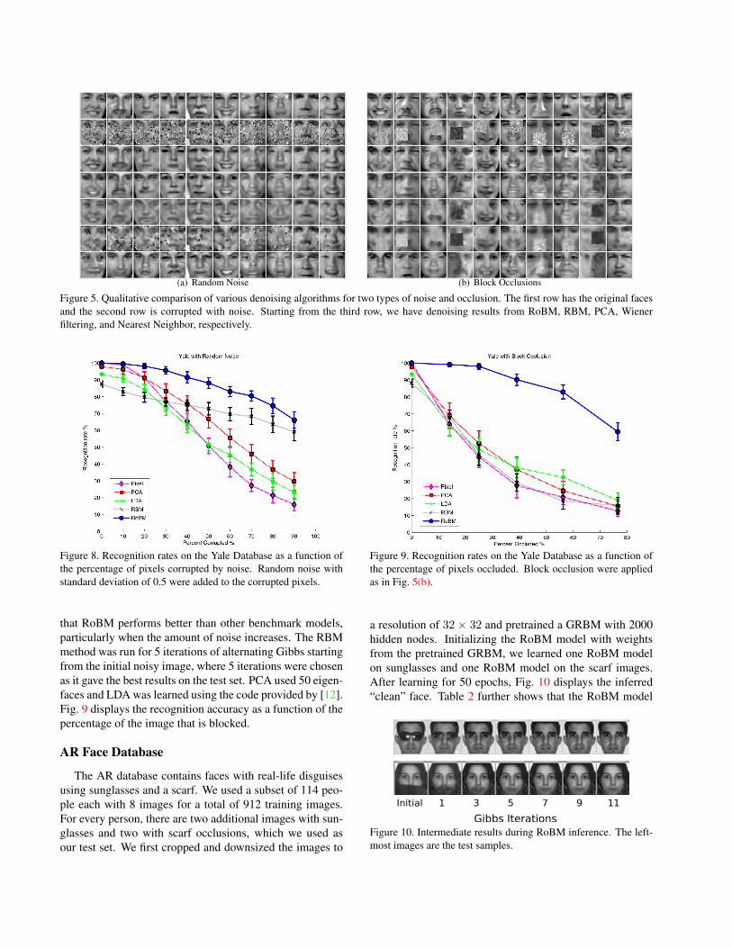
Figure 5. Qualitative comparison of various denoising algorithms for two types of noise and occlusion. The first row has the original facesand the second row is corrupted with noise. Starting from the third row, we have denoising results from RoBM, RBM, PCA, Wienerfiltering, and Nearest Neighbor, respectively.

Figure 8. Recognition rates on the Yale Database as a function ofthe percentage of pixels corrupted by noise. Random noise withstandard deviation of 0.5 were added to the corrupted pixels.

that RoBM performs better than other benchmark models,particularly when the amount of noise increases. The RBMmethod was run for 5 iterations of alternating Gibbs startingfrom the initial noisy image, where 5 iterations were chosenas it gave the best results on the test set. PCA used 50 eigen-faces and LDA was learned using the code provided by [12].Fig. 9 displays the recognition accuracy as a function of thepercentage of the image that is blocked.

AR Face Database

The AR database contains faces with real-life disguisesusing sunglasses and a scarf. We used a subset of 114 peo-ple each with 8 images for a total of 912 training images.For every person, there are two additional images with sun-glasses and two with scarf occlusions, which we used asour test set. We first cropped and downsized the images to

Figure 9. Recognition rates on the Yale Database as a function ofthe percentage of pixels occluded. Block occlusion were appliedas in Fig. 5(b).

a resolution of 32 × 32 and pretrained a GRBM with 2000hidden nodes. Initializing the RoBM model with weightsfrom the pretrained GRBM, we learned one RoBM modelon sunglasses and one RoBM model on the scarf images.After learning for 50 epochs, Fig. 10 displays the inferred“clean” face. Table 2 further shows that the RoBM model

Figure 10. Intermediate results during RoBM inference. The left-most images are the test samples.

significantly outperforms all other models on the AR facerecognition task.

Algorithms Sunglasses ScarfRoBM 84.5 % 80.7 %RBM 61.7 % 32.9 %Eigenfaces 66.9 % 38.6 %LDA 56.1 % 27.0 %Pixel 51.3 % 17.5 %

Table 2. Recognition results on the AR Face Database.

4. ConclusionsWe have described a novel model which allows Boltz-

mann Machines to be robust to noise and occlusions. Byfirst training on noise-free images followed by unsupervisedlearning on noisy images, our model can learn the structure

of the noise which allows it to perform much better on facedenoising and recognition tasks.

References[1] The yale face database., 2006. http://cvc.yale.edu/

projects/yalefaces/yalefaces.html. 4[2] S. Geman and D. Geman. Stochastic relaxation, gibbs dis-

tributions, and the bayesian restoration of images. PAMI,PAMI-6(6):721–741, 1984. 3

[3] N. Heess, N. L. Roux, and J. Winn. Weakly supervised learn-ing of foreground-background segmentation using maskedRBMs. In International Conference on Artificial Neural Net-

works (2011), July 19 2011. 1[4] G. E. Hinton and R. Salakhutdinov. Reducing the dimension-

ality of data with neural networks. Science, 313:504–507,2006. 2

[5] P. J. Huber. Robust Statistics. Wiley series in probability andmathematical statistics. John Wiley & Sons, Inc., 1981. 3

[6] H. J. Jia and A. M. Martinez. Face recognition with occlu-sions in the training and testing sets. In IEEE Int. Conf. on

Automatic Face and Gesture Recognition, 2008. 1[7] A. Kannan, N. Jojic, and B. J. Frey. Generative model for

layers of appearance and deformation. In AISTATS, 2005,2005. 1

[8] A. Krizhevsky. Learning multiple layers of features fromtiny images, 2009. 2

[9] Y. LeCun, Y. Bengio, and P. Haffner. Gradient-based learn-ing applied to document recognition. Proceedings of the

IEEE, 86(11):2278–2324, Nov. 1998. 1[10] H. Lee, R. Grosse, R. Ranganath, and A. Y. Ng. Convolu-

tional deep belief networks for scalable unsupervised learn-ing of hierarchical representations. In Intl. Conf. on Machine

Learning, pages 609–616, 2009. 2[11] D. G. Lowe. Distinctive image features from scale-invariant

keypoints. International Journal of Computer Vision, 60:91–110, 2004. 1

[12] J. Lu, K. N. Plataniotis, and A. N. Venetsanopoulos. Facerecognition using kernel direct discriminant analysis algo-rithms. IEEE-NN, 14:117–126, Jan. 2003. 6, 7

[13] A. Martınez and R. Benavente. The ar face database, Jun1998. 4

[14] A. Mohamed, G. Dahl, and G. Hinton. Acoustic modelingusing deep belief networks. IEEE Transactions on Audio,

Speech, and Language Processing, 2011. 1, 2[15] M. Ranzato, J. Susskind, V. Mnih, and G. Hinton. On Deep

Generative Models with Applications to Recognition. InCVPR, 2011. 1

[16] S. Roth and M. J. Black. Fields of experts: A framework forlearning image priors. In IEEE Conf. on Computer Vision

and Pattern Recognition, pages 860–867, 2005. 3[17] N. L. Roux, N. Heess, J. Shotton, and J. M. Winn. Learning

a generative model of images by factoring appearance andshape. Neural Computation, 23(3):593–650, 2011. 1

[18] P. Smolensky. Information processing in dynamical systems:Foundations of harmony theory. In D. E. Rumelhart andJ. L. McClelland, editors, Parallel Distributed Processing,volume 1, chapter 6, pages 194–281. MIT Press, Cambridge,1986. 2

[19] J. Susskind. The Toronto Face Database. Technical report,2011. http://aclab.ca/users/josh/TFD.html.4, 5

[20] M. Svensen and C. M. Bishop. Robust bayesian mixturemodelling. Neurocomputing, 64:235–252, 2005. 3

[21] Y. Tang. Gated Boltzmann Machine for recognition un-der occlusion. In NIPS Workshop on Transfer Learning by

Learning Rich Generative Models, 2010. 1[22] G. W. Taylor, R. Fergus, Y. LeCun, and C. Bregler. Convo-

lutional learning of spatio-temporal features. In ECCV 2010.Springer, 2010. 2

[23] T. Tieleman. Training restricted boltzmann machines usingapproximations to the likelihood gradient. In Intl. Conf. on

Machine Learning, volume 307, pages 1064–1071, 2008. 4[24] T. Tieleman and G. E. Hinton. Using fast weights to im-

prove persistent contrastive divergence. In ICML, volume382, page 130. ACM, 2009. 6

[25] M. Turk and A. P. Pentland. Eigenfaces for recognition.Journal Cognitive Neuroscience, 3(1):71–96, 1991. 6

[26] C. K. I. Williams and M. K. Titsias. Greedy learning of mul-tiple objects in images using robust statistics and factoriallearning. Neural Computation, 16(5):1039–1062, May 2004.1

[27] J. Wright, A. Y. Yang, A. Ganesh, S. S. Sastry, andY. Ma. Robust face recognition via sparse representation.IEEE Trans. Pattern Analysis and Machine Intelligence,31(2):210–227, Feb. 2009. 1

[28] L. Younes. On the convergence of markovian stochastic algo-rithms with rapidly decreasing ergodicity rates. In Stochas-

tics and Stochastics Models, pages 177–228, 1998. 4[29] Z. Zhou, A. Wagner, H. Mobahi, J. Wright, and Y. Ma. Face

recognition with contiguous occlusion using markov randomfields. In ICCV, pages 1050–1057. IEEE, 2009. 1