CSC321 Tutorial 9: Review of Boltzmann machines and ...yueli/CSC321_UTM_2014_files/tut9.pdfh1 h2...
21
CSC321 Tutorial 9: Review of Boltzmann machines and simulated annealing (Slides based on Lecture 16-18 and selected readings) Yue Li Email: [email protected] Wed 11-12 March 19 Fri 10-11 March 21
Transcript of CSC321 Tutorial 9: Review of Boltzmann machines and ...yueli/CSC321_UTM_2014_files/tut9.pdfh1 h2...

CSC321 Tutorial 9:Review of Boltzmann machines and simulated
annealing
(Slides based on Lecture 16-18 and selected readings)
Yue LiEmail: [email protected]
Wed 11-12 March 19Fri 10-11 March 21

Outline
Boltzmann Machines
Simulated Annealing
Restricted Boltzmann Machines
Deep learning using stacked RBM

General Boltzmann Machines [1]
v1 v2
h1 h2
• Network is symmetrically connected
• Allow connection between visible andhidden units
• Each binary unit makes stochasticdecision to be either on or off
• The configuration of the network dictatesits “energy”
• At the equilibrium state of the network,the likelihood is defined as theexponentiated negative energy known asthe Boltzmann distribution
Boltzmann Distribution
v1 v2
h1 h2
E (v,h) =∑i
sibi +∑i<j
si sjwij (1)
P(v) =
∑h exp(−E (v,h))∑v,h exp(−E (v,h))
(2)
where v and h are visible and hidden units,wij ’s are connection weights b/w visible-visible,hidden-hidden, and visible-hidden units,E (v,h) is the energy function
Two problems:
1. Given wij , how to achieve thermal equilibrium of P(v,h) overall possible network config. including visible & hidden units
2. Given v, learn wij to maximize P(v)

Thermal equilibrium
A
B
C
A
B
C
Transition probabilities*
at high temperature T:
AA B C
B0.01 0.02
C0.1 0.02 0.10.1 0.2 0.01
0.1
Transition probabilities*
at low temperature T
AA B C
B1e-2 1e-4
C1e-9 0.3 01e-8 1e-3 0.01
1e-3
*unnormalized probabilities (illustration only)
Thermal equilibrium is a difficult concept (Lec 16):
• It does not mean that the system has settled down into thelowest energy configuration.
• The thing that settles down is the probability distribution overconfigurations.

Simulated annealing [2]
Scale Boltzmann factor by T (“temperature”):
P(s) =exp(−E (s)/T )∑s exp(−E (s)/T )
∝ exp(−E (s)/T ) (3)
where s = {v,h}.At state t + 1, a proposed state s∗ is compared with current statest :
P(s∗)
P(st)= exp
(−E (s∗)− E (st)
T
)= exp
(−∆E
T
)(4)
st+1 ←
{s∗, if ∆E < 0 or exp(−∆E/T ) > rand(0,1)
st otherwise(5)
NB: T controls the stochastic of the transition:when ∆E > 0, T ↑⇒ exp(−∆E/T ) ↑; T ↓⇒ exp(−∆E/T ) ↓

A nice demo of simulated annealing from Wikipedia:
http://www.cs.utoronto.ca/~yueli/CSC321_UTM_2014_
files/Hill_Climbing_with_Simulated_Annealing.gif
Note: simulated annealing is not used in the Restricted BoltzmannMachine algorithm discussed below. Instead, Gibbs sampling isused. Nonetheless, it is still a nice concept and has been used inmany many other applications (the paper by Kirkpatrick et al.(1983) [2] has been has been cited for over 30,000 times based onGoogle Scholar!)

Learning weights from Boltzmann Machines is difficult
P(v) =N∏
n=1
∑h exp(−E (v,h))∑v,h exp(−E (v,h))
=∏n
∑h exp(−
∑i sibi −
∑i<j si sjwij)∑
v,h exp(−∑
i sibi −∑
i<j si sjwij)
logP(v) =∑n
(log∑h
exp(−∑i
sibi −∑i<j
si sjwij)
− log∑v,h
exp(−∑i
sibi −∑i<j
si sjwij))
∂ logP(v,h)
∂wij=∑n
(∑si ,sj
si sjP(h|v)−∑si ,sj
si sjP(v,h))
=< si sj >data − < si sj >model
where < x > is the expected value of x . si , sj ∈ {v,h}. < si sj >model is
difficult or takes long time to compute.

Restricted Boltzmann Machine (RBM) [3]
• A simple unsupervised learning module;
• Only one layer of hidden units and one layer of visible units;
• No connection between hidden units nor between visible units(i.e. a special case of Boltzmann Machine);
• Edges are still undirected or bi-directional
e.g., an RBM with 2 visible and 3 hidden units:
inputv2
h3h2h1
v1
hidden

Objective function of RBM - maximum likelihood:
E (v,h|θ) =∑ij
wijvihj +∑i
bivi +∑j
bjhj
p(v|θ) =N∏
n=1
∑h
p(v,h|θ) =N∏
n=1
∑h exp(−E (v,h|θ))∑v,h exp(−E (v,h|θ))
log p(v|θ) =N∑
n=1
log∑h
exp(−E (v,h|θ))− log∑v,h
exp(−E (v,h|θ))
∂ log p(v|θ)
∂wij=
N∑n=1
vi∑h
hjp(h|v)−∑v,h
vihjp(v,h)
= Edata[vihj ]− Emodel[vi hj ] ≡< vihj >data − < vi hj >model
But < vi hj >model is still too large to estimate, we apply MarkovChain Monte Carlo (MCMC) (i.e., Gibbs sampling) to estimate it.

<vihj>0 <vihj>
1 <vihj>∞
i
j
i
j
i
j
i
j
t = 0 t = 1 t = 2 t = infinity
<vihj>0 <vihj>
1
i
j
i
j
t = 0 t = 1 reconstruction data
a fantasy
shortcut
∂log p(v0)
∂wij=< h0j (v0
i − v1i ) > + < v1
i (h0j − h1j ) > + < h1j (v1i − v2
i ) > + . . .
=< v0i h
0j > − < v∞
i h∞j >≈< v0i h
0j > − < v1
i h1j >

How Gibbs sampling works
<vihj>0 <vihj>
1
i
j
i
j
t = 0 t = 1 reconstruction data
1. Start with a training vectoron the visible units
2. Update all the hidden unitsin parallel
3. Update all the visible unitsin parallel to get a“reconstruction”
4. Update the hidden unitsagain
∆wij = ε(< v0i h0j > − < v1i h
1j >) (6)

Approximate maximum likelihood learning
∂ log p(v)
∂wij≈ 1
N
N∑n=1
[v(n)i h
(n)j − v
(n)i h
(n)j
](7)
where
• v(n)i is the value of i th visible (input) unit for nth training case;
• h(n)j is the value of j th hidden unit;
• v(n)i is the sampled value for the i th visible unit or the
negative data generated based on h(n)j and wij ;
• h(n)i is the sampled value for the j th hidden unit or the
negative hidden activities generated based on v(n)i and wij ;
Still how exactly the negative data and negative hiddenactivities are generated?

wake-sleep algorithm (Lec18 p5)
1. Positive (“wake”) phase (clamp the visible units with data):
• Use input data to generate hidden activities:
hj =1
1 + exp(−∑
i viwij − bj)
Sample hidden state from Bernoulli distribution:
hj ←
{1, if hj > rand(0,1)
0, otherwise
2. Negative (“sleep”) phase (unclamp the visible units from data):
• Use hj to generate negative data:
vi =1
1 + exp(−∑
j wijhj − bi )
• Use negative data vi to generate negative hidden activities:
hj =1
1 + exp(−∑
i viwij − bj)

RBM learning algorithm (con’td) - Learning
∆w(t)ij = η∆w
(t−1)ij + εw (
∂ log p(v|θ)
∂wij− λw (t−1)
ij )
∆b(t)i = η∆b
(t−1)i + εvb
∂ log p(v|θ)
∂bi
∆b(t)j = η∆b
(t−1)j + εhb
∂ log p(v|θ)
∂bj
where
∂ log p(v|θ)
∂wij≈ 1
N
N∑n=1
[v(n)i h
(n)j − v
(n)i h
(n)j
]∂ log p(v|θ)
∂bi≈ 1
N
N∑n=1
[v(n)i − v
(n)i
]∂ log p(v|θ)
∂bj≈ 1
N
N∑n=1
[h(n)j − h
(n)j
]

Deep learning using stacked RBM on images [3]
2000 top-level units
500 units
500 units
28 x 28
pixel
image
10 label units
This could be the
top level of
another sensory
pathway
• A greedy learning algorithm
• Bottom layer encode the28× 28 handwritten image
• The upper adjacent layer of500 hidden units are usedfor distributedrepresentation of the images
• The next 500-units layer andthe top layer of 2000 unitscalled “associative memory”layers, which haveundirected connectionsbetween them
• The very top layer encodesthe class labels with softmax

• The networktrained on 60,000training casesachieved 1.25%test error onclassifying 10,000MNIST testingcases
• On the right arethe incorrectlyclassified images,where thepredictions are onthe top left corner(Figure 6, Hintonet al., 2006)

Let model generate 28× 28 images for specific class label
Each row shows 10 samples from the generative model with aparticular label clamped on. The top-level associative memory isrun for 1000 iterations of alternating Gibbs sampling (Figure 8,Hinton et al., 2006).
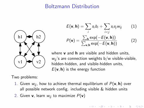
Look into the mind of the network
Each row shows 10 samples from the generative model with a particular label clamped
on. . . . Subsequent columns are produced by 20 iterations of alternating Gibbs
sampling in the associative memory (Figure 9, Hinton et al., 2006).

Deep learning using stacked RBM on handwritten images(Hinton et al., 2006)
A real-time demo from Prof. Hinton’s webpage:http://www.cs.toronto.edu/~hinton/digits.html

Further References
David H Ackley, Geoffrey E Hinton, and Terrence J Sejnowski.A learning algorithm for boltzmann machines.Cognitive science, 9(1):147–169, 1985.
S. Kirkpatrick, C. D. Gelatt, and M. P. Vecchi.Optimization by simulated annealing.Science, 220(4598):671–680, 1983.
G Hinton and S Osindero.A fast learning algorithm for deep belief nets.Neural computation, 2006.