Risk Pricing over Alternative Investment Horizons ∗

Lars Peter Hansen

University of Chicago and the NBER

June 19, 2012

Abstract

I explore methods that characterize model-based valuation of stochastically grow-

ing cash flows. Following previous research, I use stochastic discount factors as a

convenient device to depict asset values. I extend that literature by focusing on

the impact of compounding these discount factors over alternative investment hori-

zons. In modeling cash flows, I also incorporate stochastic growth factors. I explore

dynamic value decomposition (DVD) methods that capture concurrent compound-

ing of a stochastic growth and discount factors in determining risk-adjusted values.

These methods are supported by factorizations that extract martingale components

of stochastic growth and discount factors, These components reveal which ingredients

of a model have long-term implications for valuation. The resulting martingales im-

ply convenient changes in measure that are distinct from those used in mathematical

finance, and they provide the foundations for analyzing model-based implications for

the term structure of risk prices. As an illustration of the methods, I re-examine

some recent preference based models. I also use the martingale extraction to re-

visit the value implications of some benchmark models with market restrictions and

heterogenous consumers.

∗I thank Rui Cui, Mark Hendricks, Eric Renault, Grace Tsiang and especially Fernando Alvarez forhelpful discussions in preparing this chapter.

1

1 Introduction

Model-based asset prices are represented conveniently using stochastic discount factors.

These discount factors are stochastic in order that they simultaneously discount the future

and adjust for risk. Hansen and Richard (1987), Hansen and Jagannathan (1991), Cochrane

(2001) and Singleton (2006) and show how to construct and use stochastic discount factors

to compare implications of alternative asset pricing models.

This chapter explores three interrelated topics using stochastic discount factors. First

I explore the impact of compounding stochastic discount factors over alternative invest-

ment horizons required for pricing asset payoff over multi-period investment horizons. The

impact of compounding with state dependent discounting is challenging to characterize

outside the realm of log-normal models. I discuss methods that push beyond log-linear

approximations to understand better valuation differences across models over alternative

investment horizons. They allow for nonlinearities in the underlying stochastic evolution

of the economy. As an important component to my discussion, I show how to use ex-

plicit models of valuation to extract the implications that are durable over long-horizons

by deconstructing stochastic discount factors in revealing ways.

State dependence in the growth of cash flows provides a second source of compounding.

Second, I explore ways to characterize the pricing of growth rate risk by featuring the inter-

action between state dependence in discounting and growth. To support this aim I revisit

the study of holding-period returns to cash flows over alternative investment horizons, and I

suggest a characterization of the “term-structure of risk prices” embedded in the valuation

of cash flows with uncertain growth prospects. I obtain this second characterization by

constructing elasticities that show how expected returns over different investment horizons

respond to changes in risk exposures. Risk premia reflect both the exposure to risk and

the price of that exposure. I suggest ways to quantify both of these channels of influence.

In particular, I extend the concept of risk prices used to represent risk-return tradeoffs to

study multi-period pricing and give a more complete understanding of alternative structural

models of asset prices. By pricing the exposures of the shocks to the underlying macroe-

conomy, I provide a valuation counterparts to impulse response functions used extensively

in empirical macroeconomics.

In addition to presenting these tools, I also explore ways to compare explicit economic

models of valuation. I consider models with varied specifications of investor preferences and

beliefs including models with habit persistent preferences, recursive utility preferences for

2

which the intertemporal composition of risk matters, preferences that capture ambiguity

aversion and concerns for model misspecification. I also explore how the dynamics of

cross-sectional distribution of consumption influence valuation when complete risk sharing

through asset markets is not possible. I consider market structures that acknowledge private

information among investors or allow for limited commitment. I also consider structures

that allow for solvency constraints and the preclusion of financial market contracting over

idiosyncratic shocks.

The remainder of this chapter is organized as follows. In section 2 I suggest some

valuable characterizations of stochastic discount factor dynamics. I accomplish this in part

by building a change of measure based on long-term valuation considerations in contrast

to the familiar local risk-neutral change of measure. In section 3 I extend the analysis by

introducing a stochastic growth functional into the analysis. This allows for the interaction

between stochastic components to discounting and growth over alternative investment or

payoff horizons. I illustrate the resulting dynamic value decomposition (DVD) methods

using some illustrative economies that feature the impact of investor preferences on asset

pricing. Finally in section 4, I consider some benchmark models with frictions to assess

which frictions have only short-term consequences for valuation.

3

2 Stochastic discount factor dynamics

In this section we pose a tractable specification for stochastic discount factor dynamics that

includes many of the parametric specifications in the literature. I then describe methods

that characterize the implied long-term contributions to valuation and explore methods

that help us characterize impact of compounding stochastic discount factors over multiple

investment horizons.

2.1 Basic setup

I begin with an information set F0 (sigma algebra) two random vectors: Y0 and X0 that are

F0 measurable. I consider an underlying stochastic process (Y,X) = {(Yt, Xt) : t = 0, 1, ...}and use this process to define an increasing sequence of information sets (a filtration)

{Ft : t = 0, 1, ...} where (Yu, Xu) is measurable with respect to Ft for 0 ≤ u ≤ t. Following

Hansen and Scheinkman (2012b), I assume a recursive structure to the underlying stochastic

process:

Assumption 2.1. The conditional distribution (Yt+1−Yt, Xt+1) conditioned on Ft depends

only on Xt and is time invariant.

It follows from this assumption that Y does not “Granger cause” X, that X is itself a

Markov process and that {Yt+1−Yt} is a sequence of independent and identically distributed

random vectors conditioned on the entire X process.1

I suppose that the processes that we use in representing asset values have a recursive

structure.

Definition 2.2. An additive functional is a process whose first-difference has the form:

At+1 − At = κ(Yt+1 − Yt, Xt+1).

It will often be convenient to initialize the additive functional: A0 = 0, but we allow for

other initial conditions as well. I model stochastic growth and discounting using additive

functionals after taking logarithms. This specification is flexible enough to include many

commonly-used time series models. I relate the first-difference of A to the first-difference of

Y in order to allow the increment in A to depend on the increment in Y in continuous-time

counterparts.

1For instance, see Bickel et al. (1998). I may think of this conditional independence as being morerestrictive counterpart to Sims (1972)’s alternative characterization of Granger (1969) causality.

4

2.2 A convenient factorization

Let St denote the stochastic discount factor between dates zero and t. The implicit dis-

counting over a single time period between t and t + 1 is embedded in this specification

and is given by ratio St+1

St. The discounting is stochastic to accommodate risk adjustments

in valuation. In representative consumer models with power utility functions

St+1

St= exp(−δ)

(Ct+1

Ct

)−ρ(1)

where Ct is aggregate consumption at date t, δ is the subjective rate of discount, and 1ρ

is

the elasticity of intertemporal substitution. The formula on the right-hand side of (1) is

the one-period intertemporal marginal rate of substitution for the representative consumer.

This particular formulation is very special and problematic from an empirical perspective,

but I will still use it as revealing benchmark for comparison.

One-period stochastic discount factors have been used extensively to characterize the

empirical support, or lack thereof, for understanding one-period risk return tradeoffs. My

aim, however, to explore valuation for alternative investment horizons. For instance, to

study the valuation of date t + 2 payoffs from the vantage point of date t, I am lead to

compound two one-period stochastic discount factors:(St+2

St+1

)(St+1

St

)=St+2

St

Extending this logic leads me to the study of the stochastic discount factor process S, which

embeds the stochastic discounting for the full array of investment horizons.

Alvarez and Jermann (2005), Hansen et al. (2008), Hansen and Scheinkman (2009) and

Hansen (2012) suggest, motivate and formally defend a factorization of the form:

St+1

St= exp(−η)

(Mt+1

Mt

)[f(Xt+1)

f(Xt)

](2)

where M is a martingale and X is a Markov process. I will show subsequently how to

construct f . I will give myself flexibility in how I normalize S0. While sometimes I will

set it to one, any strictly positive normalization will suffice. In what follows we suppose

that both logS and logM are additive functionals. Extending this formula to multiple

5

investment horizons:StS0

= exp(−ηt)(Mt

M0

)[f(Xt)

f(X0)

]. (3)

There are three components to the this factorization, terms that I will interpret after

I supply some more structure. Notice that each of the logarithms of each of the three

components are themselves additive functionals.

I construct factorization (2) by solving the Perron-Frobenius problem:

E

[(St+1

St

)e(Xt+1)|Xt = x

]= exp(−η)e(x) (4)

where e is a positive function of the Markov state. Then

Mt

M0

= exp(ηt)

(StS0

)[e(Xt)

e(X0)

]is a martingale. Inverting this relation: gives (3) with f = 1

e.

The preceding construction is not guaranteed to be unique. See Hansen and Scheinkman

(2009) and Hansen (2012) for discussions. Recall that positive martingales with unit ex-

pectations can be used to induce alternative probability measures via a formula

E (Mtψt|F0) = E (ψt|Ft)

for any bounded ψt that is in the date t information set (is Ft measurable). It is straight-

forward to show that under this change-of-measure, the process X remains Markov and

that Assumption 2.1 continue to hold. This martingale construction is not guaranteed to

be unique, however. There is at most one such construction for which the martingale M

induces stochastically stable dynamics where stochastic stability requires:

Assumption 2.3. Under the change of probability measure,

limt→∞

E [φ(Yt − Yt−1, Xt)|X0 = x] = E[φ(Yt − Yt−1, Xt)]

for any bounded Borel measurable function φ. The expectation on the right-hand side uses

a stationary distribution implied by the change in the transition distribution.2

2One way to characterize the stationary distribution is to solve E [ψ(X0)M0] =

E(E [ψ(X1)|X0 = x]M0

).

6

See Hansen and Scheinkman (2009) and Hansen (2012) for discussions. There is a well

developed set of tools for analyzing Markov processes that can be leveraged to check this

restriction. See Meyn and Tweedie (1993) for an extensive discussion of these methods.

The version of factorization (2) that preserves this stochastic stability is of interest for

the following reason. It allow me to compute:

E [Stφ(Yt − Yt−1, Xt)|X0 = x] = exp(−ηt)e(x)E

[φ(Yt − Yt−1, Xt)

e(Xt)|X0 = x

]Under stochastic stability,

limt→∞

1

tlogE [Stφ(Yt − Yt−1, Xt)|X0 = x] = −η (5)

limt→∞

logE [Stφ(Yt − Yt−1, Xt)|X0 = x] + ηt = log e(x) + log E

[φ(Yt − Yt−1, Xt)

e(Xt)

]provided that φ > 0. Thus the change-in-probability absorbs the martingale component to

stochastic discount factors. The rate η is the long-term interest rate, which is evident from

(5) when we set φ to be a function that is identically one.3

2.3 Other familiar changes in measure

In the pricing of derivative claims, researchers often find it convenient to use the so called

“risk neutral” measure. To construct this in discrete time, form

Mt+1

Mt

=St+1

E (St+1|Ft).

Then M is a martingale with expectation equal to one provided that EM0 = 1. An

alternative stochastic discount factor is:

St+1

St=

(Mt+1

Mt

)E

(St+1

St|Ft). (6)

3I have added sufficient structure as to provide a degenerate version of the Dybvig et al. (1996) charac-terization of long-term rates. Dybvig et al. (1996) argue that long-term rates should be weakly increasing.

7

The risk-neutral probability is the probability measure associated with the martingale M ,

and the one-period interest rate on a discount bond is:

− logE

(St+1

St|Ft).

Absorbing the martingale into the change of measure, the one period prices are compute by

discounting using the riskless rate, justifying the term “risk-neutral measure.” Whenever

the one-period interest rate is state independent, it is equal to η; and factorizations (2) and

(6) coincide with e = f = 1 (or some other positive constant).

When interest rates are expected to vary over time, this variation in effect gives an

adjustment for risk over multiple investment horizons. An alternative would be to use a

different change of measure for each investment horizon, but this is not very convenient

conceptually.4 Instead I find it preferable to use a single change of measure with a constant

adjustment to the long-term decay rate η in the stochastic discount factor that is state

independent as in (2).

2.4 Log-linear models

It is commonplace to extract permanent shocks as increments in martingale components of

time series. This approach is related but distinct from the approach that I have sketched.

The connection is closest when the underlying model of a stochastic discount factor is

log-linear with normal shocks. See Alvarez and Jermann (2005) and Hansen et al. (2008).

Suppose that

logSt+1 − logSt = −µ+H ·Xt +G ·Wt+1

Xt+1 = AXt +BWt+1

where W is a multivariate sequence of standard normally distributed random vectors with

mean zero and covariance I and A is a matrix with stable eigenvalues (eigenvalues with

absolute values that are strictly less than one). In this case we can construct a martingale

component m in logarithms and

logSt − logS0 = −νt+mt −m0 + f ·Xt − h ·X0

4Such changes in measure are sometimes called forward measures. See Jamshidian (1989) for an initialapplication of these measures.

8

where m is a an additive martingale satisfying:

mt+1 −mt =[G′ +H ′(I − A)−1B

]Wt+1,

and

f ·Xt = −H ′(I − A)−1Xt.

Increments to the additive martingale are permanent shocks, and shocks that are uncorre-

lated have only transient consequences.

While m is an additive martingale, exp(m) is not a martingale. It is straightforward to

construct the martingale M by forming

Mt

M0

= exp(mt −m0) exp

[− t

2|G′ +H ′(I − A)−1B|2

]where the second term adjusts is a familiar log-normal adjustment. With stochastic volatil-

ity models or regime-shift models, the construction is not as direct. See Hansen (2012) for a

discussion of a more general link be between martingale constructions for additive processes

and factorization (3).5

2.5 Model-based factorizations

Factorization (3) provides a way to formalize long-term contributions to valuation. Consider

two alternative stochastic discount factor processes, S and S∗ associated with two different

models of valuation.

Definition 2.4. The valuation implications between model S and S∗ are transient if

these processes share a common value of the long-term interest rate η and the martingale

component M .

Consider the factorization (3) for the power utility model mentioned previously:

S∗t = exp(−δt)(CtC0

)−ρ= exp(−η∗t)

(M∗

t

M∗0

)[f ∗(Xt)

f ∗(X0)

](7)

where δ is the subjective rate of discount, ρ > 0, and(CtC0

)−ρis the (common) intertemporal

5The martingale extraction in logarithms applies to a much larger class of processes and results in anadditive functional. The exponential of the resulting martingale shares a martingale component in thelevel factorization (3) with the original process.

9

marginal rate of substitution of an investor between dates zero and t. I assume that logC

satisfies Assumption 2.1. It follows immediately the the logarithm of the marginal utility

process, γ logC satisfies this same restriction. In addition the function f ∗ = 1e∗

and (e∗, η∗)

solves the eigenvalue equation (4) including the imposition of stochastic stability.

Suppose for the moment we hold fixed the consumption process as a device to under-

stand the implications of changing preferences. Bansal and Lehmann (1997) noted that

the stochastic discount factors for many asset pricing models have a common structure. I

elaborate below. The one-period ratio of the stochastic discount factor is:

St+1

St=

(S∗t+1

S∗t

)[h(Xt+1)

h(Xt)

]. (8)

From this baseline factorization,

StS0

= exp(−ηt)(Mt

M0

)[f(Xt)h(Xt)

f(X0)h(X0)

].

The counterpart for the eigenfunction e is 1f∗h

. Thus when factorization (8) is satisfied,

the long-term interest rate η and the martingale component to the stochastic discount

factor are the same as those with power utility. The function h contributes “transient”

components to valuation. Of course these transient components could be highly persistent.

While my aim is to provide a more full characterization of the impact of the payoff

horizon on the compensation for exposure to risk, locating permanent components to models

of valuation provides a good starting point. It is valuable to know when changes in modeling

ingredients has long-term consequences for valuation and when these changes are more

transient in nature. It is also valuable to understand when “transient changes” in valuation

persist over long investment horizons even though the consequences eventually vanish. The

classification using martingale components is merely an initial step for a more complete

understanding.

I now explore the valuation implications of some alternative specifications of investor

preferences.

2.5.1 Consumption externalities and habit persistence

See Abel (1990), Campbell and Cochrane (1999), Menzly et al. (2004) and Garcia et al.

(2006) for representations of stochastic discount factors in the form (8) for models with

history dependent measures of consumption externalities. A related class of models are

10

those in which there are intertemporal complementaries in preferences of the the type

suggested by Sundaresan (1989), Constantinides (1990) and Heaton (1995). As argued

by Hansen et al. (2008) these models also imply stochastic discount factors that can be

expressed as in (8).

2.5.2 Recursive utility

Consider a discrete-time specification of recursive preferences of the type suggested by

Kreps and Porteus (1978) and Epstein and Zin (1989). I use the homogeneous-of-degree-

one aggregator specified in terms of current period consumption Ct and the continuation

value Vt for prospective consumption plan from date t forwards:

Vt =[(ζCt)

1−ρ + exp(−δ) [Rt(Vt+1)]1−ρ] 1

1−ρ . (9)

where

Rt (Vt+1) =(E[(Vt+1)

1−γ|Ft]) 1

1−γ

adjusts the continuation value Vt+1 for risk. With these preferences, 1ρ

is the elasticity of

intertemporal substitution and δ is a subjective discount rate. The parameter ζ does not

alter preferences, but gives some additional flexibility, and we will select it in a judicious

manner. The stochastic discount factor S for the recursive utility model satisfies:

St+1

St= exp(−δ)

(Ct+1

Ct

)−γ [Vt+1/Ct+1

Rt (Vt+1/Ct)

]ρ−γ. (10)

The presence of the next-period continuation value in the one-period stochastic discount

factor introduces a forward-looking component to valuation. It gives a channel by which

investor beliefs matter. I now explore the consequences of making the forward-looking

contribution to the one-period stochastic discount factor as potent as possible in a way

that can be formalized mathematically. This relevant for the empirical literature as that

literature is often led to select parameter configurations that feature the role of continuation

values.

Following Hansen (2012) and Hansen and Scheinkman (2012b), we consider the following

equation:

E

[(Ct+1

Ct

)1−γ

e(Xt+1)|Xt = x

]= exp(η)e(x).

11

Notice that this eigenvalue equation has the same structure as (4) with (Ct)1−γ taking the

place of St. The formula for the stochastic discount factor remains well defined in the

limiting case as we let (ζ)1−ρ tend to zero and δ decreases to6

1− ρ1− γ − 1

η.

ThenVtCt≈ [e(Xt)]

1−γ ,

and

St ≈ exp(−ηt)(CtC0

)−γ [e(Xt)

e(X0)

] ρ−γ1−γ

. (11)

Therefore, in the limiting case

h(x) = e(x)ρ−γ1−γ

in (8).

2.5.3 Altering martingale components

Some distorted belief models of asset pricing feature changes that alter the martingale

components. As I have already discussed, positive martingales with unit expectations imply

changes in the probability distribution. They act as so-called Radon-Nikodym derivatives

for changes that are absolutely continuous over any finite time interval. Suppose that N is

a martingale for which logN is an additive functional. Thus

E

(Nt+1

Nt

|Xt = x

)= 1.

This martingale captures investors beliefs that can be distinct from those given by the

underlying model specification. Since Assumption 2.1 is satisfied, for the baseline specifi-

cation, it may be shown that the alternative probability specification induced by the mar-

tingale N also satisfies the assumption. This hypothesized difference between the model

and the beliefs of investors is presumed to be permanent with this specification. That

is, investors have confidence in this alternative model and do not, for instance consider a

mixture specification while attempting to infer the relative weights using historical data.

6Hansen and Scheinkman (2012b) use the associated change of measure to show when existence to thePerron-Frobenius problem implies the existence of a solution to the fixed point equation associated withan infinite-horizon investor provided that δ is less than this limiting threshold.

12

For some distorted belief models, the baseline stochastic discount factor S∗ from power

utility is altered by the martingale used to model the belief distortion:

S = S∗N.

Asset valuation inherits the distortion in the beliefs of the investors. Consider factorization

(7) for S∗. Typically NM∗ will not be a martingale even though both components are

martingales. Thus to obtain the counterpart factorization for a distorted belief economy

with stochastic discount factor S requires that we extract a the martingale component from

NM∗. Belief changes of this type have permanent consequences for asset valuation.

Examples of models with exogenous belief distortions that can be modeled in this way

include Cecchetti et al. (2000) and Abel (2002). Related research by Hansen et al. (1999),

Chen and Epstein (2002), Anderson et al. (2003) and Ilut and Schneider (2012) uses a

preference for robustness to model misspecification and ambiguity aversion to motivate

explicitly this pessimism.7 In this literature the form of the pessimism is an endogenous

response to investors’ uncertainty about which among a class of model probability specifi-

cations governs the dynamic evolution of the underlying state variables. The martingale N

is not their “actual belief” rather the outcome of exploring the utility consequences of con-

sidering an array of probability models. Typically there is a benchmark model that is used,

and we take the model that we have specified without distortion as this benchmark. In

these specifications, the model uncertainty does not vanish over time via learning because

investors are perpetually reluctant to embrace a single probability model.

2.5.4 Endogenous responses

So far our discussion has held fixed the consumption process in order to simplify the impact

of changing preferences. Some stochastic growth models with production have a balanced

growth path relative to some stochastically growing technology. In such economies, some

changes in preferences, while altering consumption allocations, may still preserve the mar-

tingale component along with the long-term interest rate.

7There is a formal link between some recursive utility specifications and robust utility specifications thathas origins in the control theory literature on risk-sensitive control. Anderson et al. (2003) and Maenhout(2004) develop these links in models of portfolio choice and asset pricing.

13

2.6 Entropy characterization

In the construction that follows we build on ideas from Bansal and Lehmann (1997), Al-

varez and Jermann (2005), and especially Backus et al. (2011). The relative entropy of a

stochastic discount factor functional S for horizon t is given by:

1

t[logE (St|X0 = x)− E (logSt|X0 = x)] ,

which is nonnegative as an implication of Jensen’s Inequality. When St is log-normal,

this notion of entropy yields one-half the conditional variance of logSt conditioned on

date zero information, and Alvarez and Jermann (2005) propose using this measure as

a “generalized notion of variation.” Backus et al. (2011) study this measure of relative

entropy averaged over the initial state X0. They view this entropy measure for different

investment horizons as an attractive alternative to the volatility of stochastic discount

factors featured by Hansen and Jagannathan (1991). To relate these entropy measures to

asset pricing models and data, Backus et al. (2011) note that

−1

tE [logE (St | X0)]

is the average yield on a t-period discount bond where we use the stationary distribution

for X0. Following Bansal and Lehmann (1997),

−1

tE (logSt) = −E (logS1) ,

is the average one-period return on the maximal growth portfolio under the same distribu-

tion.

Borovicka and Hansen (2012) derive a more refined quantification of how entropy de-

pends on the investment horizon t given by

1

t[logE (St | X0)− E (logSt | X0)] =

1

t

t∑j=1

E [ς(Xt−j, j) | X0] . (12)

The right-hand side represents the horizon t entropy in terms of averages of the building

blocks ς(x, t) where

ς(x, t) = logE [St | X0 = x]− E [logE (St | F1) | X0 = x] ≥ 0.

14

The term ς is itself a measure of “entropy” of

E(St | F1)

E(St | F0)

conditioned on date zero information and measures the magnitude of new information that

arrives between date zero and date one for St. For log-normal models, ς(x, t) is one half

the variance of E (logSt | F1)− E (logSt | F0).

15

3 Cash-flow pricing

Rubinstein (1976) pushed us to think of the asset pricing implications from a multi-period

perspective in which an underlying set of future cash flows are priced. I adopt that vantage

point here. Asset values can move either because market-determined stochastic discount

rates have altered (a price change), or because the underlying claim implies a higher or lower

cash flow (a quantity change). These two channels motivate formal methods for enhancing

our understanding of what economic models have to say about present-value relations. One

common approach uses log-linear approximation to identify two (correlated) sources of time

variation in the ratio of an asset value to the current period cash flow. The first source

is time variation in expected returns to holding the asset, a price effect; and the second is

time variation in expected dividend growth rates, a quantity effect. Here I explore some

more broadly applicable methods to produce “dynamic valuation decompositions” which

are complementary to the log-linear approach. My aim is to unbundle the pricing of cash

flows in revealing ways. The specific impetus for this formulation comes form the work of

Lettau and Wachter (2007) and Hansen et al. (2008), and the general formulation follows

Hansen and Scheinkman (2009) and Hansen (2012).

3.1 Incorporating stochastic growth in the cash flows

Let G be a stochastic growth factor where logG satisfies Assumption 2.1. Notice that if

logG and logS both satisfy this assumption, their sum does as well. While the stochastic

discount factor decays over time, the stochastic growth factor grows over time. I will

presume that discounting dominates and that the product SG is expected to decay over

time. I consider cash flows of the type:

Gt+1φ(Yt+1 − Yt, Xt+1) (13)

where G0 is in the date zero information set F . The date t value of this cash flow is:

E

[St+1

S0

Gt+1φ(Yt+1 − Yt, Xt+1)|F0

]= G0E

[St+1Gt+1

S0G0

φ(Yt+1 − Yt, Xt+1)|X0

].

16

An equity sums the values of the cash flows at all dates t = 1, 2, .... By design we may

compute values recursively repeatedly applying a one-period valuation operator:

Vh(x) = E

[St+1Gt+1

StGt

h(xt+1)|Xt = x

].

Let

h(x) = E

[St+1Gt+1

StGt

φ(Yt+1 − Yt, Xt+1)|Xt = x

].

Then

E

[St+1

S0

Gt+1φ(Yt+1 − Yt, Xt+1)|F0

]= G0Vth(x).

To study cash flow pricing with stochastic growth factors, we use a factorization of the

type given in (3) but applied to SG instead of S:

StGt

S0G0

= exp(−ηt)(Mt

M0

)[f(Xt)

f(X0)

]where f = 1

eand e solves:

E

[(St+1Gt+1

StGt

)e(Xt+1|Xt = x

]= exp(−η)e(x).

The factorization of SG cannot be obtained by factoring S andG separately and multiplying

the outcome because products of martingales are not typically martingales. Thus co-

dependence matters.8

3.2 Holding-period returns on cash flows

A return to equity with cash flows or dividends that have stochastic growth components can

be viewed as a bundle or portfolios of holding period returns on cash flows with alternative

payout dates. (See Lettau and Wachter (2007) and Hansen et al. (2008).) The gross

one-period holding-period return over a payoff horizon t is:(G1

G0

)(Vt−1[h(X1)]

Vt[h(X0)]

).

8When S and G are jointly lognormally distributed, we may first extract martingale components of logSand logG and add these together and exponentiate. While this exponential will not itself be a martingale,we may construct a positive martingale by multiplying this exponential by a geometrically declining scalefactor.

17

Changing the payoff date t changes the exposure through a valuation channel as reflected

by the second term in brackets, while the direct cash flow channel reflected by the first

term remains the same as we change the payoff horizon.

To characterize the holding-period return for large t, I apply the change in measure and

represent this return as:

exp(η)G1

G0

[e(X1)

e(X0)

](E[h(Xt)f(Xt)|X1]

E[h(Xt)f(Xt)|X0]

)

The last term converges to unity as the payoff horizon τ increases, and the first two terms

do not depend on τ . Thus the limiting return is:(G1

G0

)[exp(η)

e(X1)

e(X0)

]. (14)

The valuation component is now tied directly to the solution to the Perron-Frobenius

problem. An eigenfunction ratio captures the state dependence. In addition there is an

exponential adjustment η, which is in effect a value-based measure of duration of the cash

flow G and is independent of the Markov state. When η is near zero, the cash flow values

deteriorate very slowly as the investment horizon is increased.

The study of holding-period returns on cash flows payoffs over alternative payoff dates

gives one way to characterize a valuation dynamics. Recent work by van Binsbergen et al.

(2011) and van Binsbergen et al. (2012) develop and explore empirical counterpart to these

returns. Next I appeal to ideas from price theory to give a different depiction.

3.3 Shock elasticities

Next I develop valuation counterparts to impulse-response functions commonly used in the

study of dynamic, stochastic equilibrium models. I refer to these counterparts as shock

elasticities. As I will show, these elasticities measure both exposure and price sensitivity

over alternative investment horizons.

As a starting point, consider a cash flow G and stochastic discount factor S. For

investment horizon t, form the logarithm of the expected return to this cash flow given by:

logE

[(Gt

G0

)|X0 = x

]− logE

[(Gt

G0

)(StS0

)|X0 = x

]

18

where the scaling by G0 is done for convenience. The first term is the logarithm of the

expected payoff and the second term is the logarithm of the price. To measure the risk-

premium I compare this expected return to a riskless investment over the same time horizon.

This is a special case of my previous calculation in which I set Gt = 1 for all t. Thus the

logarithm of this returns is:

− logE

[(StS0

)|X0 = x

]I measure the risk premium by comparing these two investments:

risk premium = logE

[(Gt

G0

)|X0 = x

]− logE

[(Gt

G0

)(StS0

)|X0 = x

]+ logE

[(StS0

)|X0 = x

]. (15)

In what follows I will study the value implications as measured by what happens to the

risk premium when I perturb the exposure of the cash flow to the underlying shocks.

To unbundle value implications, I borrow from price theory by computing shock price

and shock exposure elasticities. (I think of an exposure elasticity as the counterpart to

a quantity elasticity.) In so doing I build on the continuous-time analyses of Hansen

and Scheinkman (2012a) and Borovicka et al. (2011) and on the discrete-time analysis of

Borovicka and Hansen (2012). To simplify the interpretation, suppose there is an underlying

sequence of iid multivariate standard normally distributed shocks {Wt+1}. Introduce:

logHt+1(r)− logHt(r) = rσ(Xt) ·Wt+1 −(r)2

2|σ(Xt)|2

where I assume that

E[|σ(Xt)|2

]= 1

and logH0(r) = 0. Here I use σ(x) to select the combination of shocks that is of interest

and I scale this state-dependent vector in order that σ(Xt) · Wt+1 has a unit standard

deviation.9

Also I have constructed the increment in logHt+1 so that

E

[Ht+1(r)

Ht(r)|Xt = x

]= 1.

9Borovicka et al. (2011) suggest counterpart elasticities for discrete states modeled as Markov processes.

19

I use the resulting process H(r) to define a scalar family of martingale perturbations pa-

rameterized by r.

Consider a cash flow G that may grow stochastically over time. By multiplying G by

H(r), I alter the exposure of the cash flow to shocks. Since I am featuring small changes,

I am led to use the process:

Dt+1 −Dt = σ(Xt) ·Wt+1

with D0 = 0 to represent two exposure elasticities:

εe(x, t) =d

dr

1

tlogE

[Gt

G0

Ht(r)|X0 = x

]∣∣∣∣r=0

=1

t

E[GtG0Dt|X0 = x

]E[GtG0|X0 = x

]εe(x, t) =

d

drlogE

[Gt

G0

H1(r)|X0 = x

]∣∣∣∣r=0

= σ(X0)E[GtG0W1|X0 = x

]E[GtG0|X0 = x

] .

These elasticities depend both on the investment horizon t and the current value of the

Markov state x. For a fixed horizon t, the first of these elasticities, which I call a risk-price

elasticity, changes the exposure at all horizons. The second one concentrates on changing

only the first period exposure, much like an impulse response function.10 As argued by

Borovicka et al. (2011) and Borovicka and Hansen (2012), the risk price-elasticities are

weighted averages of the shock-price elasticities.

The long-term limit (as t→∞) of the shock-price elasticity has a tractable character-

ization. Consider a factorization of the form (3), but applied to G. Using the martingale

from this factorization, Borovicka and Hansen (2012) show that

limt→∞

E[GtG0W1|X0 = x

]E[GtG0|X0 = x

] = E [W1|X0 = x] .

10Under log-normality there is a formal equivalence between our elasticity and an impulse responsefunction.

20

As intermediate calculations, I also compute:

εv(x, t) =d

dr

1

tlogE

[StGt

S0G0

Ht(r)|X0 = x

]∣∣∣∣r=0

=1

t

E[StGtS0G0

Dt|X0

]E[StGtS0G0|X0

]εv(x, t) =

d

drlogE

[StGt

S0G0

H1(r)|X0 = x

]∣∣∣∣r=0

=E[StGtS0G0

D1|X0

]E[StGtS0G0|X0

] .

which measure the sensitivity of value to changes in the exposure. These elasticities in-

corporate both a change in price and a change in exposure. The implied risk-price and

shock-price elasticities are given by:

εp(x, t) = εe(x, t)− εv(x, t)

εp(x, t) = εe(x, t)− εv(x, t).

In what follows I draw on some illustrations from the existing literature.

3.3.1 Lettau-Wachter example

Lettau and Wachter (2007) consider an asset pricing model of cash-flow duration. They

use an ad hoc model of a stochastic discount factor to display some interesting patterns

of risk premia. When thinking about the term structure of risk premia, I find it useful to

distinguish pricing implications from exposure implications. Both can contribute to risk

premia as a function of the investment horizon.

Lettau and Wachter (2007) explore implications of a cash flow process with linear dy-

namics:

Xt+1 =

[.9658 0

0 .9767

]Xt +

[.12 0 0

0 −.0013 .0009

]Wt+1

where {Wt+1} is iid multivariate standard normally distributed. They model the logarithm

of the cash flow process as

logGt+1 − logGt = µg +X[2]t +

[0 .0724 0

]Wt+1

where X[2]t is the second component of Xt. I compute shock exposure elasticities, which

in this case are essentially the same as impulse response functions for logG since the cash

21

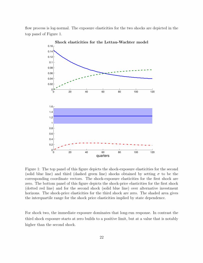
flow process is log-normal. The exposure elasticities for the two shocks are depicted in the

top panel of Figure 1.

Shock elasticities for the Lettau-Wachter model

0 20 40 60 80 100 1200

0.02

0.04

0.06

0.08

0.1

0.12

0.14

0.16

0 20 40 60 80 100 1200

0.2

0.4

0.6

0.8

1

1.2

1.4

1.6

quarters

Figure 1: The top panel of this figure depicts the shock-exposure elasticities for the second(solid blue line) and third (dashed green line) shocks obtained by setting σ to be thecorresponding coordinate vectors. The shock-exposure elasticities for the first shock arezero. The bottom panel of this figure depicts the shock-price elasticities for the first shock(dotted red line) and for the second shock (solid blue line) over alternative investmenthorizons. The shock-price elasticities for the third shock are zero. The shaded area givesthe interquartile range for the shock price elasticities implied by state dependence.

For shock two, the immediate exposure dominates that long-run response. In contrast the

third shock exposure starts at zero builds to a positive limit, but at a value that is notably

higher than the second shock.

22

Next we assign “prices” to the shock exposures. The stochastic discount factor in

Lettau-Wachter model evolves as:

logSt+1 − logSt = −r −(.625 +X

[1]t

) [0 1 0

]Wt+1 −

|.625 +X[1]t |2

2.

Nonlinearity is present in this model because the conditional mean of logSt+1 − logSt is

quadratic in X[1]t . This is a model with a constant interest rate r and state dependent

one-period shock price vector:

(.625 +X[1]t )

0

1

0

.By assumption only the second shock commands a nonzero one-period shock price elasticity

and this elasticity varies over time. The process {.625 + X[1]t } is a stochastic volatility

process that induces movements in the shock price elasticities. In its stationary distribution,

this process has a standard deviation of .46 and hence varies substantially relative to its

mean of .625. The first shock alters the first component of Xt and the shock-price elasticity

for the first shock is different from zero after one period. The cash flow G does not respond

to this shock so the “pricing” of the first component of W[1]t+1 does not play a direct role in

the valuation of G.11

The shock-price elasticities are depicted in the bottom panel of Figure 1. A consequence

of the specification of the stochastic discount factor S is that the second shock has a constant

(but state dependent) shock-price elasticity of .625 + X[1]t as a function of the investment

horizon. This shock has the biggest impact for the cash flow, and it commands the largest

shock price elasticity elasticity both immediately and over the long term. Thus, I have

shown that this application of dynamic value decomposition reveals that the impetus for

the downward risk premia as a function of horizon comes from the dynamics of the cash-flow

shock exposure and not from the price elasticity of that exposure.

We now shift to a different specification of preferences and cash flows, and show what

this same methods reveal in a different context.

11Lettau and Wachter (2007) use this model to interpret the differential expected returns in growth andvalue stocks. Value stocks are more exposed to the second shock .

23

3.3.2 Recursive utility

We illustrate pricing implications for the recursive utility model using a specification from

Hansen et al. (2007) of a “long-run risk” model for consumption dynamics featured by

Bansal and Yaron (2004). Bansal and Yaron (2004) use historical data from the United

States to motivate their model including the choice of parameters. Their model includes pre-

dictability in both conditional means and in conditional volatility. We use the continuous-

time specification from Hansen et al. (2007) because the continuous-time specification of

stochastic volatility is more tractable:

dX[1]t = −.021X

[1]t dt+

√X

[2]t

[.00031 −.00015 0

]dWt,

dX[2]t = −.013(X

[2]t − 1)dt+

√X

[2]t

[0 0 −.038

]dWt

d logCt = .0015dt+X[1]t dt+

√X

[2]t

[.0034 0.007 0

]dWt,

where W is a trivariate standard Brownian motion. The unit of time in this time series

specification is one month, although for comparability with other models I plot shock-price

elasticities using quarters as the unit of time. The first component of the state vector is

the state dependent component to the conditional growth rate, and the second component

is a volatility state. Both the growth state and the volatility state are persistent. We

follow Hansen (2012) in configuring the shocks for this example. The first one is the

“permanent shock” identified using standard time series methods and normalized to have

a unit standard deviation. The second shock is a so-called temporary shock, which by

construction is uncorrelated with the first shock.

Our analysis assumes a discrete-time model. A continuous-time Markov process X ob-

served at say interval points in time remains a Markov process in discrete time. Since

logCt+1 − logCt is constructed via integration, it is not an exact function of Xt+1 and

Xt. To apply our analysis, we define Yt+1 = logCt+1 − logCt. Given the continuous-time

Markov specification, the joint distribution of logCt+1 − logCt and Xt+1 conditioned on

past information only depends on the current Markov state Xt as required by Assumption

2.1.12 The resulting shock-price elasticities are reported in Figure 2 for the three different

shocks. Since the model with power utility (ρ = γ = 8) has preferences that are additively

separable, the pricing impact of a permanent shock or a stochastic-volatility shock accu-

12I exploit the continuous-time quasi analytical formulas given by Hansen (2012) for the actual compu-tations.

24

mulates over time with the largest shock-price elasticities at the large investment horizon

limit. In contrast, recursive utility with (ρ = 1, γ = 8) has an important forward-looking

component for pricing.13 As a consequence, the trajectory for the shock-price elasticities

for the permanent shock and for the shock to stochastic volatility are much flatter than for

the power utility model, and in particular, the short-term shock price elasticity is relatively

large for the permanent shock to consumption.

The presence of stochastic volatility induces state dependence in all of the the shock-

price elasticities. This dependence is reflected in the shaded portions in Figure 2 and of

particular interest for the permanent shock, and its presence is a source of time variation

in the elasticities for each of the investment horizons.

The amplification of the short-term shock price elasticities has been emphasized at the

outset in the literature on “long run risk” through the guises of the recursive utility model.

Figure 2 provides a more complete picture of cash risk pricing. The fact the limiting

behavior for recursive and power utility specifications are in agreement follow from the

factorization (11).

Models with external habit persistence provide a rather different characterization of

shock price elasticities as I will now illustrate.

3.3.3 External habit models

Borovicka et al. (2011) provide a detailed comparison of the pricing implications of two

specifications of external habit persistence, one given in Campbell and Cochrane (1999)

and the other in Santos and Veronesi (2006). In order to make the short-term elasticities

comparable, Borovicka et al. (2011) modified the parameters for the Santos and Veronesi

(2006) model. Borovicka et al. (2011) performed their calculations using a continuous-time

specification in which consumption is a random walk with drift when specified in logarithms.

Thus, in contrast to the “long-run risk model”, the consumption exposure elasticities are

constant.

d logCt = .0054dt+ .0054dWt

whereW is a scalar standard Brownian motion and the numerical value of µc is inconsequen-

tial to our calculations. I will not elaborate on the precise construction of the social habit

stock used to model the consumption externality and instead posit the implied stochas-

13See Hansen (2012) for a discussion of the sensitivity to the parameter ρ, which governs the intertemporalelasticity of substitution.

25

Shock-price elasticities for recursive utility model

0 20 40 60 80 100 1200

.2

.4

.6Permanent price elasticity

0 20 40 60 80 100 1200

.2

.4

.6Temporary price elasticity

0 20 40 60 80 100 1200

0.05

0.1

0.15

0.2

quarters

Volatility price elasticity

Figure 2: This figure depicts the shock-price elasticities of the three shocks for a modelwith power utility (ρ = γ = 8) depicted by the dashed red line and with recursive utility(ρ = 1, γ = 8) depicted by the solid blue line. The shaded region gives the interquartilerange of the shock price elasticities induced by state dependence for the recursive utilitymodel.

tic discount factors. The constructions differ and are delineated in the respective papers.

Rather than embrace a full structural interpretation of the consumption externality, I will

focus on the specification of the stochastic discount factors for the two models.

26

For Santos and Veronesi (2006), the stochastic discount factor is

StS0

= exp(−δt)(CtC0

)−2Xt + 1

X0 + 1

where

dXt = −.035(Xt − 2.335)dt− .496dWt.

Thus the shock to dXt is proportional to the shock to d logCt with the same magnitude but

opposite sign. In our calculations we set G = C. Consequently, the martingale component

to the stochastic discount factor is given by

Mt

M0

= exp

[(.0054)Wt −W0 −

t

2(.0054)2

]and the Perron-Frobenius eigenfunction is e(x) = 1

x+1.

For Campbell and Cochrane (1999), the stochastic discount factor is

StS0

= exp(−δt)(CtC0

)−2exp(2Xt)

exp(2X0)

where

dXt = −.035(Xt − .4992) +(

1−√

1 + 1200Xt

)dWt.

In this case the Perron-Frobenius eigenfunction is e(x) = exp(−2x). The martingale com-

ponents of S are the same for the two models, as are the martingale components for SG.

Figure (3) depicts the shock-price elasticities for the two models for the quartiles of the

state distribution. While the starting points and limit points for the shock-price trajecto-

ries agree, there is a substantial difference how fast the trajectories approach their limits.

The long-term limit point is the same as that for a power utility specification (ρ = γ = 2).

For the Santos and Veronesi (2006) specification, the consumption externality is arguably

a transient model component. For the Campbell and Cochrane (1999) specification, this

externality has very durable pricing implications even if formally speaking this model fea-

ture is transient. The nonlinearities in the state dynamics apparently compound in a rather

different manner for the two specifications. See Borovicka et al. (2011) for a more extensive

comparison and discussion.

These examples all feature models with directly specified consumption dynamics. While

this has some pedagogical simplicity for comparing impact of investor preferences on asset

27

Shock-price elasticities for the external habit model

0 20 40 60 80 100 1200

0.1

0.2

0.3

0.4

0.5

0.6

0 20 40 60 80 100 1200

0.1

0.2

0.3

0.4

0.5

0.6

quarters

Figure 3: This figure depicts the shock-price elasticities for this single shock specification ofthe models with consumption externalities. The top panel displays the shock-price elasticityfunction in the Santos and Veronesi (2006) specification, while the bottom panel displaysthe Campbell and Cochrane (1999) specification. The solid curve conditions on the medianstate, while the shaded region depicts the interquartile range induced by state dependence.

prices, it is of considerable interest to apply these dynamic value decomposition (DVD)

methods to a richer class of economies including economies with multiple capital stocks. For

example, Borovicka and Hansen (2012) apply the methods to study a production economy

with “tangible” and “intangible” capital as modeled in Ai et al. (2010). Richer models will

provide scope for analyzing the impact of shock exposures with more interesting economic

interpretations.

28

The elasticities displayed here are local in nature. They feature small changes in ex-

posure to normally distributed shocks. For highly nonlinear models, global alternatives

may well have some appeal; or at the very least alternative ways to alter exposure to

non-gaussian tail risk.

29

4 Market Restrictions

I now explore the stochastic discount factors that emerge from some benchmark economies

in which there is imperfect risk sharing. In part, my aim is to provide a characterization

about how these economies relate to the more commonly used structural models of asset

pricing. The cross-sectional distribution of consumption matters in these examples, and

this presents interesting challenges for empirical implementation. While acknowledging

these challenges, my goal is to understand how these distributional impacts are encoded in

asset prices over alternative investment horizons.

I study some alternative benchmark economies with equilibrium stochastic discount

factor increments that can be expressed as:

St+1

St=

(Sat+1

Sat

)(Sct+1

Sct

)(16)

where the first-term on the right-hand side,Sat+1

Sat, coincides with that of a representative

consumer economy and the second term,Sct+1

Sct, depends on the cross-sectional distribution

of consumption relative an average or aggregate. In the examples that I explore,

Sat+1

Sat= exp(−δ)

(Cat+1

Cat

)−ρwhere Ca denotes aggregate consumption. The way in which Sc depends on the cross section

differs in the example economies that I discuss because the market restrictions differ. As in

the literature that I discuss, I allow the cross-sectional distribution of consumption (relative

to an average) to depend on aggregate states.

While a full characterization of the term structure implications for risk prices is a worthy

goal, here I will only initiate such a discussion by investigating when these limits on risk

sharing lead to “transient” vs. “permanent” implications for market values. In one case

below, Sct = f(Xt) for some (Borel measurable) function f of a stochastically stable process

X. Thus we know that introducing market imperfections has only transient consequences.

For the other examples, I use this method to indicate what are the sources within the model

for long-term influence of cross-sectional consumption distributions on asset values.

30

4.1 Incomplete contracting

Our first two examples are economies in which there are aggregate, public shocks and

idiosyncratic, private shocks. Payoffs can be written on the public shocks but not on the

private shocks. Let Gt denote the sigma algebra that includes both public and private

shocks, and let Ft denote the sigma algebra that includes only public shocks. By forming

expectations of date t random variables that are Gt measurable conditioned on Ft, we

aggregate over the idiosyncratic shocks but condition on the aggregate shocks. We use this

device to form cross-sectional averages. I presume that that

E (Qt+1|Gt) = E (Qt+1|Ft)

whenever Qt+1 is Ft measurable. There could be time invariant components to the speci-

fication of Gt, components that reflect an individual’s type.

In what follows I use Ct to express consumption in a manner that implicitly includes

dependence on idiosyncratic shocks. Thus Ct is Gt measurable. Thus the notation Ct

includes a specification of consumption allocated to a cross section of individuals at date

t. With this notation, aggregate consumption is:

Cat = E (Ct|Ft) . (17)

As an example, following Constantinides and Duffie (1996) consider consumption allo-

cations of the type:

logCt+1 − logCt = logCat+1 − logCa

t + Vt+1Zt+1 −1

2(Zt+1)

2 (18)

where Vt+1 is Gt+1 measurable and a standard normally distributed random variable condi-

tioned on composite event collection: Gt ∨Ft+1. The random variable Zt+1 is in the public

information set Ft+1. It now suffices to define the cross-sectional average

Ca0 = E [C0|F0] ,

then (17) is satisfied because

E

(exp

[Vt+1Zt+1 −

1

2(Zt+1)

2

]| Gt ∨ Ft+1

)= 1.

31

In this example since Vt+1 is an idiosyncratic shock, the idiosyncratic contribution to aggre-

gate consumption has permanent consequences the aggregate random variable Zt+1 shifts

the cross sectional consumption distribution. Shortly we will discuss a decentralization that

accompanies this distribution for which aggregate uncertainty in the cross-sectional distri-

bution of consumption matters for valuation. This is just an example, and more general

and primitive starting points are of interest.

In what follows, to feature the role of market structure we assume a common discounted

power utility function for consumers ρ = γ. The structure of the argument is very similar

to that of Kocherlakota and Pistaferri (2009), but there are some differences.14 Of course

one could “add on” a richer collection of models of investor preferences, and for explaining

empirical evidence there may be good reason to do so. To exposit the role of market

structure, I focus on a particularly simple specification of consumer preferences.

4.1.1 Trading assets that depend only on aggregate shocks

First I consider a decentralized economy in which heterogenous consumers trade securities

with payoffs that only depend on the aggregate states. Markets are incomplete because

consumers cannot trade

I introduce a random variable Qt+1 that is Ft+1 measurable. Imagine adding rQt+1 to

the t+ 1 consumption utilities. The date t price of the payoff rQt+1 is

rE

[(St+1

St

)Qt+1 | Ft

],

which must be subtracted from the date t consumption. The scalar r can be Gt measurable.

We consider an equilibrium allocation for C, and thus part of the equilibrium restriction is

that r = 0 be optimal. This leads to the first-order conditions:

(Ct)−ρE

[(St+1

St

)Qt+1 | Ft

]= exp(−δ)E

[(Ct+1)

−ρQt+1 | Gt]. (19)

In order to feature the cross sectional distribution of consumption, I construct:

ct =CtCat

.

14The decentralization of the private information Pareto optimal allocation exploits in a part a derivationprovided to me by Fernando Alvarez.

32

I divide both sides by (Cat )−ρ:

(ct)−ρE

[(St+1

St

)Qt+1 | Ft

]= exp(−δ)E

[(ct+1)

−ρ(Cat+1

Cat

)−ρQt+1 | Gt

].

I consider two possible ways to represent the stochastic discount factor increment. First

divide by the (scaled) marginal utility (ct)−ρ and apply the Law of Iterated Expectations:

E

[(St+1

St

)Qt+1 | Ft

]= exp(−δ)E

[(ct+1

ct

)−ρ(Cat+1

Cat

)−ρQt+1 | Ft

].

By allowing trades among assets that include any bounded payoff that is Ft+1 measurable,

it follows thatSt+1

St= exp(−δ)

(Cat+1

Cat

)−ρE

[(ct+1

ct

)−ρ| Ft+1

]. (20)

See Appendix A. This generalizes the usual power utility model representative agent spec-

ification of the one-period stochastic discount factor. Because of the preclusion of trading

based on idiosyncratic shocks, investors equate the conditional expectations of their in-

tertemporal marginal rates of substitution conditioned only on aggregate shocks. This

gives one representation of the limited ability to share risks with this market structure.

For an alternative representation, use the Law of Iterated Expectations on both the left

and right-hand sides of (19) to argue that

E[(ct)

−ρ|Ft]E

[(St+1

St

)Qt+1 | Ft

]= exp(−δ)E

(E[(ct+1)

−ρ | Ft+1

](Cat+1

Cat

)−ρQt+1 | Ft

)

Again I use the flexibility to trade based on aggregate shocks to claim that

St+1

St= exp(−δ)

(Cat+1

Cat

)−ρ E [(ct+1)−ρ | Ft+1

]E[(ct)

−ρ | Ft] . (21)

For specification (18) suggested by Constantinides and Duffie (1996), ct+1− ct is condition-

ally log-normally distributed and as a consequence,

E

[(ct+1

ct

)−ρ| Ft+1

]= exp

[ρ(ρ+ 1)(Zt+1)

2

2

]

33

In this special case,

St+1

St= exp(−δ)

(Cat+1

Cat

)−ρexp

[ρ(ρ+ 1)(Zt+1)

2

2

].

This is just an example, but an informative one. The consumption distribution “fans out”

and its dependence on the aggregate state variable Zt+1 implies permanent consequences

for the the stochastic discount factor.15 There are other mechanisms that might well push

against the fanning which are abstracted from in this formulation. For instance, overlap-

ping generations models can induce some reversion depending on how the generations are

connected and how new generations are endowed.

4.1.2 Efficient Allocations with Private Information

One explicit rationale for limiting contracting to aggregate shocks is that idiosyncratic

shocks reflect private information. In an interesting contribution, Kocherlakota and Pista-

ferri (2007, 2009) propose a decentralization of constrained efficient allocations represented

via the construction of a stochastic discount factor. Kocherlakota and Pistaferri consider

the case of constraint efficient allocations where agents’ preferences are given by expected

discounted utility with an additive sub-utility of consumption and leisure (or effort), and

where the consumption sub-utility is specified as a power utility function, ρ = γ. Individual

agents’ leisure (effort) needed to produce a given output is private information. Individuals

cannot hide consumption, however, through even inefficient storage.

Kocherlakota and Pistaferri (2009) take as given the solution of planning problem where

agents effort is unobservable. How this efficient allocation is attained is an interesting

question in its own right, a question that is of direct interest and discussed extensively

in the literature on contracting in the presence of private information. To decentralize

these allocations, Kocherlakota and Pistaferri consider intermediaries that can observe

the consumption of the agents and that can trade among themselves. They distinguish

between aggregate shocks (which are public) and idiosyncratic shocks which are private

but diversifiable as with the incomplete financial market model that I discussed previously.

Intermediaries trade among themselves in complete markets on all public shocks and engage

15In the degenerate case in which Z is constant over time, the impact of the cross-sectional distributionwill only be to scale the stochastic discount factor and hence prices will be scaled by a common factor.Risk and shock price elasticities will coincide with those from the corresponding representative consumermodel.

34

a large number of agents so they diversify completely the privately observed shocks. The

contract of the intermediary with the agents ensures that the reports are correct. The

objective of the intermediaries is to minimize the cost, at market prices, of delivering agents

a given lifetime utility. This intermediary provides a way to deduce the corresponding

stochastic discount factor for assigning values to payoffs on the aggregate state.

I introduce a random variable Qt+1 that is Ft+1 measurable. Imagine adding rQt+1 to

the t + 1 period utilities instead to the period t + 1 consumption. Due to the additive

separability of the period utility function adding an amount of utils both on t and across

all continuations at t+ 1 does change the incentives for the choice of leisure (effort). This

leads me to consider the equivalent adjustment ∆t+1(r) to consumption:

rQt+1 + U(Ct+1) = U [Ct+1 + ∆t+1(r)] .

I have altered the t+1 period cross-sectional utility in a way that is equivalent to changing

the utility to the efficient allocation of consumption in the cross sectional distribution at

date t+ 1 in a manner that does not depend on the idiosyncratic shocks. To support this

change, however, the change in consumption ∆t+1(r) does depend on idiosyncratic shocks.

Differentiating with respect to r:

Qt+1 = (Ct+1)−ρ ∆t+1

dr

∣∣∣∣r=0

.

Thusd∆t+1

dr

∣∣∣∣r=0

= Qt+1(Ct+1)ρ.

To compensate for the rQt+1 change in the next period (date t+ 1) utility, subtract

exp(−δ)E (Qt+1|Gt) = exp(−δ)E (Qt+1|Gt)

from the current (date t) utility. This leads me to solve:

−r exp(−δ)E(Qt+1|Ft) + U(Ct) = U [Ct −Θt(r)].

Again differentiating with respect to r,

− exp(−δ)E(Qt+1|Ft) = (Ct)−ρ dΘt

dr

∣∣∣∣r=0

,

35

ordΘt

dr

∣∣∣∣r=0

= exp(−δ)E(Qt+1|Ft)(Ct)ρ

The members of our family of rQt+1 perturbations have the same continuation values as

those in the efficient allocation. By design the perturbations are equivalent to a transfer

of utility across time periods that does not depend on idiosyncratic shocks. These two

calculations are inputs into first-order conditions for the financial intermediary.

The financial intermediary solves a cost minimization problem:

minr−E [Θt(r)|Ft] + E

[(St+1

St

)∆t+1(r)|Ft

].

We want the minimizing solution to occur when r is set to zero. The first-order conditions

are:

−E[dΘt

dr

∣∣∣∣r=0

|Ft]

+ E

[(St+1

St

)d∆t+1

dr

∣∣∣∣r=0

|Ft]

= 0.

Substituting for the ∆t and Θt derivatives,

− exp(−δ)E(Qt+1|Ft)E [(Ct)ρ|Ft] + E

[(St+1

St

)Qt+1E [(Ct+1)

ρ|Ft+1] |Ft]

= 0. (22)

Let

Dt+1 = exp(δ)

(St+1

St

)(Ca

t+1)ρE [(ct+1)

ρ|Ft+1]

(Cat )ρE [(ct)ρ|Ft]

where I have used the fact that the cross-sectional averages Cat and Ca

t+1 are in the respective

information sets of aggregate variables. Then

E(Qt+1|Ft) = E [Dt+1Qt+1|Ft]

Given flexibility in the choice of the Ft+1 measurable random variable Qt+1, I show in

Appendix A that Dt+1 = 1, giving rise to the “inverse Euler equation:”(St+1

St

)= exp(−δ)

(Cat+1

Cat

)−ρE [(ct)

ρ|Ft]E [(ct+1)ρ|Ft+1]

(23)

suggested by Kocherlakota and Pistaferri (2009). The “inverse” nature of the Euler equa-

tion emerges because my use of utility based perturbations based on aggregate shocks rather

than direct consumption-based perturbations. This type of Euler equation is familiar since

36

the seminal work of Rogerson (1985).

An alternative, but complementary analysis, derives the full solution to the constraint

efficient allocation. At least since the work of Atkeson and Lucas (1992), it is known that

even temporary idiosyncratic shocks create a persistent trend in dispersion of consumption.

Hence this particular way of modeling private information has the potential of important

effects the long-term (martingale) component to valuation.

In the incomplete contracting framework we were led to consider the time series of cross-

sectional moments {E [(ct)−ρ|Ft] : t = 1, 2, ...} whereas in this private information, Pareto

efficient economy we are led to consider {E [(ct)ρ|Ft] : t = 1, 2, ...}. These two models fea-

ture rather different attributes, including tails behavior of the cross-sectional distribution

for consumption. Both, however, suggest the possibility of long-term contributions to valu-

ation because of the dependence of the cross-sectional distribution on economic aggregates.

There are important measurement challenges that arise in exploring the empirical under-

pinnings of these models, but some valuable initial steps have been taken by Brav et al.

(2002), Cogley (2002) and Kocherlakota and Pistaferri (2009).

4.2 Solvency Constraints

In this section I discuss the representation of stochastic discount factor in models where

agents face occasionally binding solvency constraints. One tractable class of models that

features incomplete risk sharing is the one where agents have access to complete markets

but where the total value of their financial wealth is constrained (from below) in a state

contingent manner. Following Luttmer (1992, 1996) and He and Modest (1995), I refer

to such constraints as solvency constriants. In contrast to the models with incomplete

contracting based on information constraints, I no longer distinguish between Gt and Ft;but I do allow for some ex ante heterogeneity in endowments or labor income. Suppose

there are i types of investors, each with consumption Cit . Investor types may have different

initial asset holdings and may different labor income or endowment processes. Let Cat

denote the average across all consumers and cit =CitCat

. Under expected discounted utility

preferences with a power specification (ρ = γ), the stochastic discount factor increment is:

St+1

St= exp (−δ)

(Cat+1

Cat

)−ρmaxi

{(cit+1

cit

)−ρ}. (24)

37

To better understand the origin of this formula, notice that an implication of it is:

St+1

St≥ exp (−δ)

(Cit+1

Cit

)−ρ, (25)

which is featured in the work Luttmer (1992, 1996) and He and Modest (1995).

To understand better this inequality, observe that positive scalar multiples r ≥ 0 of a

positive payoff Qt+1 ≥ 0 when added to composite equilibrium portfolio payoff of person

i at date t + 1 will continue to satisfy the solvency constraint. Thus such a perturbation

is an admissible one. When I optimize with respect to r, I now impose the constraint that

r ≥ 0; and this introduces a Kuhn-Tucker multiplier into the calculation. The first-order

condition for r is

(Cit)−ρE

[(St+1

St

)Qt+1 | Ft

]≥ exp(−δ)E

[(Ci

t+1)−ρQt+1 | Ft

].

where the inequality is included in case the nonnegativity constraint on r is binding. Since

this inequality is true for any bounded, positive nonnegative Ft+1 measurable payoff Qt+1,

inequality relation (25) holds.

Formula (24) is a stronger restriction and follows since equilibrium prices are determined

by having at least one individual that is unconstrained in the different realized date t + 1

states of the world. The max operator captures the feature that the types with the highest

valuation are unconstrained. While in principle expression (24 ) can be estimated using

an empirical counterpart to the type’s i consumption, the presence of the max using error

ridden data makes the measurement daunting.

Luttmer (1992) takes a different approach by exploiting the implications via aggregation

of solvency constraints and analyzing the resulting inequality restriction.16 This same

argument is revealing for my purposes as well. Since ρ is positive, inequality (25) implies

that

Cit

(St+1

St

)− 1ρ

≤ exp(−δ)Cit+1

where inequality is reversed because −1ρ< 0. Forming a cross-sectional average, preserves

the inequality:

Cat

[exp(δ)

St+1

St

]− 1ρ

≤ Cat+1.

16See Hansen et al. (1995) for a discussion of econometric methods that support such an approach.

38

Raising both sides to the negative power −ρ reverses again the inequality:

(Cat )−ρ

[exp(δ)

St+1

St

]≥(Cat+1

)−ρ.

Rearranging terms gives the inequality of interest

St+1

St≥ exp(−δ)

(Cat+1

Cat

)−ρ. (26)

Form this inequality, we can rule out any hope that solvency-constraint models only have

transient consequences for valuation because we cannot hope to write

St+1

St= exp(−δ)

(Cat+1

Cat

)−ρ [h(Xt+1)

h(Xt)

].

for some h and some stochastically stable process X, unless of course h(X) is constant with

probability one. In the degenerate case, the solvency constraints are not binding. At the

very least the interest rate rates on discount bonds, including the long-term interest rate,

have to be smallar than those in the corresponding representative consumer economy.

Alvarez and Jermann (2000, 2001) and Chien and Lustig (2010) impose more structure

on the economic environment in order to get sharper predictions about the consumption

allocations. They use limited commitment as a device to set the solvency thresholds needed

to compute an equilibrium.17 Following Kehoe and Levine (1993), these authors introduce

an outside option that becomes operative if an investor defaults on the financial obligations.

The threat of the outside option determines the level of the solvency constraint that is

imposed in a financial market decentralization. Solvency constraints are chosen to prevent

that the utility value to staying in a market risk sharing arrangement to be at least as high as

the utility of the corresponding outside options. Alvarez and Jermann (2001) and Chien and

Lustig (2010) differ in terms the precise natures of the market exclusions that occur when

investor walk away from their financial market obligations. Alvarez and Jermann (2000)

argue that the cross-sectional distribution in example economies with solvency constraints

stable in the sense that Cit = hi(Xt)C

at for some stochastically stable Markov process X.

17Zhang (1997) considers a related environment in which borrowing constraints are endogenously deter-mined as implication of threats to default. Alvarez and Jermann (2000, 2001) and Chien and Lustig (2010)extend Zhang (1997) by introducing a richer collection of security markets.

39

ThusSt+1

St= exp(−δ)

(Cat+1

Cat

)−ρmaxi

{(hi(Xt+1)

hi(Xt)

)−ρ}.

Notice that the objective of the max operation is ratio of a common function of the Markov

state over adjacent periods. Even so, given our previous argument the outcome of this

maximization will not have an expression as an analogous ratio. Even with a stable con-

sumption allocation, the presence of solvency constraints justified by limited commitment

may have long-term consequences for valuation.18

Chien and Lustig (2010) also provide a suggestive characterization for the stochastic

discount factor ratio of the form:

St+1

St= exp(−δ)

(Cat+1

Cat

)−ρ(Zt+1

Zt

)ρ.

Thus (Zt)ρ = Sct in representation (16). Chien and Lustig interpret Z and characterize the

ratio Zt+1

Ztusing numerical methods. In particular, they show that the positive process Z

does not decrease over time.19 This property for Z is to be anticipated from (26). Unless

it is degenerate, such a process cannot be stationary; but its logarithm can have stationary

increments as presumed in my analysis.

Even though the consumption distribution may not “fan out” over time, evidently the

introduction of solvency constraints has important long-term consequences for valuation.

A remaining challenge is to understand better when the implied state dependence in the

cross-sectional distribution of individual consumption ratios induces changes in the long-

18Alvarez and Jermann (2000) derive a different type of factorization of a stochastic discount factorunder some very special restrictions. They express the endowments for each investor type as a product ofthe aggregate endowment and a share of that endowment. They suppose that the growth in the aggregateendowment is itself independent and identically distributed and that the aggregate endowment process isindependent of the vector of endowment share processes. They argue that equilibrium stochastic discountfactor is the product of the corresponding representative consumer stochastic discount factor and a termthat is independent of the process for aggregate endowment growth. (See the proof of their Proposition5.4.) Thus the two terms in factorization (16) are statistically independent in their example. The pricesof payoffs that depend only on aggregate endowment growth process over fixed investment horizon havecommon term that emerges because of the contribution of the share process history to the stochasticdiscount factor. By forming price ratios, this share-process contribution to valuation is netted out. For acash flow G that depends only on the aggregate endowment and not on the share process, the cash-flowrisk premia as measured by formula (15) will be the same as for the corresponding representative consumermodel with iid consumption growth. An analogous simplification applies to payoffs that depend only onshare process and not on the aggregate endowment.

19See also Alvarez and Jermann (2000) Proposition 5.2 for the analogous result for the limited commit-ment economies that they study.

40

term risk prices.

4.3 Segmented Market and Nominal Shocks

In this section I explore environments that feature both nominal shocks and segmented

asset markets. The transient consequences of nominal shocks has been featured in other

environments. For instance in log-linear specifications of the macro time series, Blanchard

and Quah (1989) and Shapiro and Watson (1988) use the transient nature of nominal shocks

as a device to identify tansient and permanent sources of economic fluctuations. Here I

explore economic models with explicit transition mechanisms to investigate further the

transient nature of nominal shocks for valuation including adjustments for risk exposure.

As an illustration, I consider the stylized model of Alvarez et al. (2002) and Alvarez et al.

(2009) where both nominal cash-flows and segmentation are introduced. For simplicity,

these models presume a binding cash-in-advance constraint, and hence the price level is

proportional to money supply. Consumers can transfer cash between their “brokerage

account” –where an intermediary with access to complete security markets manages their

portfolio– and a liquid asset that must be use for consumption expenditures. For consumers

to embark on this transfer, they must pay a fixed cost. If they decide not to pay the fixed

cost, they must consume the real value of the accumulated nominal income. In equilibrium

only some of the consumers participate in asset markets, but those that do so have the

same consumption, which I denote by Cpt . In this case the one-period stochastic discount

factor is given by the corresponding one-period intertemporal marginal rate of substitution

of the participants adjusted for changes in the nominal price level

St+1

St= exp(−δ)

(PtPt+1

)(Cpt+1

Cpt

)−ρwhere Pt is the date t price level and where St is the nominal discount factor. This formula

is true even though, the identity of the participants changes over time. The equilibrium of

this model is such that

Cpt = Ca

t hp(logmt − logmt−1)

where logmt − logmt−1 is the growth rate of the money supply and Cat is aggregate con-

sumption. Thus

St+1

St= exp(−δ)

(PtPt+1

)(Cat+1

Cat

)−ρ [h(logmt+1 − logmt)

h(logmt − logmt−1)

](27)

41

where h = (hp)−ρ.

In transaction cost models such as this one, the impact on risk pricing is transient rela-

tive to a standard power utility model. The impact of changes in participation is captured

by the function h of the presumed stationary growth rate in the money supply. Nominal

fluctuations influence real outcomes The factorization in (27) features both standard nom-

inal effects on valuation from both the nominal price level P , and aggregate consumption

Ca. Both contribute to the martingale component of the stochastic discount factor S. This

type of models can and has been used to study both term premium for nominal interest

rates as well for nominal exchange rates. Third, one can use the growth decomposition

described in equation (13) by letting G = P to distinguish real cash flows from nominal

ones or more generally by letting a multiplicative component of G be P as a device to

take nominal growth into account for computing real risk-price and shock price-elasticities

induced by nominal shocks.

In this section I have only “scratched the surface” so to speak on characterizing how and

when market restrictions alter the term structure of shock an risk-price elasticities through

it implications for the time series behavior of cross-sectional distributions. As a starting

point I have examined when the long-term discount rate and the martingale components

of stochastic discount factors are altered, but as I argued earlier in a different context this

is merely a starting point for a more complete analysis.

42

5 Conclusions

In this chapter I have focused on characterizing asset values through the lens of economic

models of valuation. By using structural models, models with an explicitly specified pref-

erence and market structure, researchers can assign values to a rich collection of cash flows

and risk prices for the exposures to alternative underlying macroeconomic shocks. These

DVD methods that I discussed allow researchers to extract pricing implications for cash

flows without resort to log-linearization. I consider the global “entropy” methods and local

“elasticity” methods based on perturbing the exposure of cash flows to shocks as comple-

mentary devices to characterized the sensitivity of risk prices to the investment horizon.

The DVD methods are supported in part by a factorization that provides a mathemati-

cal formalization of permanent and transitory components to valuation. The distinction

between permanent and transitory rests formally on limiting behavior when we extend

the investment horizon. As with related time series decompositions, this distinction en-

hances both model building and testing by clarifying when the permanent and transitory

distinction is sharp and when it is blurred.

While this is a chapter about models, it also suggestive of what hypothetical securi-

ties might be most useful in distinguishing among competing models. As time series data

on richer collections of equity-based derivative contracts become available, they offer the

promise to pose direct challenges to the underlying pricing of cash flows. Complemen-

tary econometric and empirical advances will enhance our understanding of the empirical

underpinnings of structural models of asset prices.

43

A Limited contracting economies revisited

In this appendix I complete two of the arguments made in Section 4.1. Consider first an

argument in 4.1.1. There I showed that

E

[(St+1

St

)Qt+1 | Ft

]= exp(−δ)E

[(ct+1

ct

)−ρ(Cat+1

Cat

)−ρQt+1 | Ft

]. (28)

My aim is to show that formula (20) is satisfied. For convenience, I rewrite it:

St+1

St= exp(−δ)

(Cat+1

Cat

)−ρE

[(ct+1

ct

)−ρ| Ft+1

].

Let

Qt+1 =

1(St+1

St

)> exp(−δ)

(Cat+1

Cat

)−ρE

[(ct+1

ct

)−ρ| Ft+1

]0 otherwise

Then it follows from (28) that

(St+1

St

)> exp(−δ)

(Cat+1

Cat

)−ρE

[(ct+1

ct

)−ρ| Ft+1

]

with probability zero. An entirely similar argument implies the reverse inequality. Thus

representation (20) is valid. Since a similar argument proves (21), I do not repeat the logic.

Consider next an argument in Section 4.1.2 Recall the construction:

Dt+1 =

(St+1

St

)exp(δ)E [(Ct+1)

ρ|Ft+1]

E [(Ct)ρ|Ft]

and the implication

E (Dt+1Qt+1|Ft) = E (Qt+1|Ft) .

I now show that by exploiting the flexibility in the choice of Zt+1, Dt+1 = 1 giving rise to

the inverse Euler equation: (23) Let

Qt+1 =

{Dt+1 if b > Dt+1 > 1

0 otherwise.

I impose an upper bound on Qt+1 to ensure that perturbation in the date t+1 utility can be

44

implemented by choices of individual consumptions. It follows that Pr {b ≥ Qt+1 > 1} = 0.

Since b is arbitrary, it must also be true that Pr {Dt+1 > 1} = 0. Similarly, form

Qt+1 =

{0 if Dt+1 ≥ 1

Dt otherwise.

It then follows that Pr {Dt+1 < 1} = 0. Thus Dt+1 = 1.

45

References

Abel, Andrew B. 1990. Asset Prices under Habit Formation and Catching up with the

Joneses. The American Economic Review 80 (2):pp. 38–42.

———. 2002. An exploration of the effects of pessimism and doubt on asset returns. Journal

of Economic Dynamics and Control 26.

Ai, Hengjie, Mariano Massimiliano Croce, and Kai Li. 2010. Toward a Quantitative General

Equilibrium Asset Pricing Model with Intangible Capital. Mimeo.

Alvarez, F., A. Atkeson, and P.J. Kehoe. 2002. Money, Interest Rates, and Exchange Rates

with Endogenously Segmented Asset Market. Journal of Political Economy 1 (110):773–

112.

———. 2009. Time-Varying Risk, Interest Rates, and Exchange Rates in General Equilib-

rium. Review of Economic Studies 76 (3):851–878.

Alvarez, Fernando and Urban Jermann. 2000. Efficiency, Equilibrium, and Asset Pricing

with Risk of Default. Econometrica 775–798.

Alvarez, Fernando and Urban J. Jermann. 2001. Quantitative Asset Pricing Implications

of Endogenous Solvency Constraints. The Review of Financial Studies 14 (4):pp. 1117–

1151.

———. 2005. Using Asset Prices to Measure the Persistence of the Marginal Utility of

Wealth. Econometrica 73 (6):pp. 1977–2016.

Anderson, Evan W., Lars Peter Hansen, and Thomas J. Sargent. 2003. A Quartet of

Semigroups for Model Specification, Robustness, Prices of Risk, and Model Detection.

Journal of the European Economic Association 1 (1):68–123.

Atkeson, A. and R.E. Jr. Lucas. 1992. On efficient distribution with private information.

The Review of Economic Studies 59 (3):427–453.

Backus, David, Mikhail Chernov, and Stanley Zin. 2011. Sources of Entropy in Represen-

tative Agent Models. Unpublished working paper.

Bansal, Ravi and Bruce N. Lehmann. 1997. Growth-optimal Portfolio Restrictions on Asset

Pricing Models. Macroeconomic Dynamics 1 (2):333–354.

46

Bansal, Ravi and Amir Yaron. 2004. Risks for the Long Run: A Potential Resolution of

Asset Pricing Puzzles. Journal of Finance 59 (4):1481–1509.

Bickel, Peter J., Ya’acov Ritov, and Tobias Ryden. 1998. Asymptotic Normality of the

Maximum-Likelihood Estimator for General Hidden Markov Models. The Annals of

Statistics 26 (4):1614–1635.

van Binsbergen, Jules, Michael Brandt, and Ralph Koijen. 2011. On the Timing and Pricing

of Dividends. American Economic Review forthcoming.

van Binsbergen, Jules, Michael Brandt, Ralph Koijen, and Evert Vrugt. 2012. Equity

Yields. Becker-Friedman Institute Working Paper.

Blanchard, Olivier Jean and Danny Quah. 1989. The Dynamic Effects of Aggregate Demand

and Supply Disturbances. The American Economic Review 79 (4):pp. 655–673.

Borovicka, Jaroslav and Lars Peter Hansen. 2012. Examining macroeconomic models

through the lens of asset pricing. Working Paper Series WP-2012-01, Federal Reserve

Bank of Chicago.

Borovicka, Jaroslav, Lars Peter Hansen, Mark Hendricks, and Jose A. Scheinkman. 2011.

Risk Price Dynamics. Journal of Financial Econometrics 9:3–65.

Brav, Alon, George M. Constantinides, and Christopher C. Geczy. 2002. Asset Pricing

with Heterogeneous Consumers and Limited Participation: Empirical Evidence. Journal

of Political Economy 110 (4):pp. 793–824.

Campbell, John Y. and John H. Cochrane. 1999. By Force of Habit. Journal of Political

Economy 107 (2):205–251.

Cecchetti, Stephen G., Pok-sang Lam, and Nelson C. Mark. 2000. Asset Pricing with

Distorted Beliefs: Are Equity Returns Too Good to Be True? The American Economic

Review 90 (4):pp. 787–805.

Chen, Zengjing and Larry Epstein. 2002. Ambiguity, Risk, and Asset Returns in Continuous

Time. Econometrica 70 (4):1403–1443.

Chien, YiLi and Hanno Lustig. 2010. The Market Price of Aggregate Risk and the Wealth

Distribution. Review of Financial Studies 23 (4):1596–1650.

47

Cochrane, John H. 2001. Asset Pricing. Princeton, N.J.: Princeton University Press.

Cogley, Timothy. 2002. Idiosyncratic risk and the equity premium: evidence from the

consumer expenditure survey. Journal of Monetary Economics 49 (2):309 – 334.

Constantinides, George M. 1990. Habit Formation: A Resolution of the Equity Premium

Puzzle. Journal of Political Economy 98 (3):519–43.

Constantinides, George M. and Darrell Duffie. 1996. Asset Pricing with Heterogeneous

Agents. Journal of Political Economy 104 (2):219–240.

Dybvig, Philip H., Jr. Ingersoll, Jonathan E., and Stephen A. Ross. 1996. Long Forward

and Zero-Coupon Rates Can Never Fall. The Journal of Business 69 (1).

Epstein, L. and S. Zin. 1989. Substitution, Risk Aversion and the Temporal Behavior of

Consumption and Asset Returns: A Theoretical Framework. Econometrica 57 (4):937–

969.

Garcia, Rene, Eric Renault, and Andrei Semenov. 2006. Disentangling risk aversion and

intertemporal substitution through a reference level. Finance Research Letters 3:181–193.

Granger, C. W. J. 1969. Investigating Causal Relations by Econometric Models with Cross-

spectral Methods. Econometrica 37:424–438.

Hansen, Lars Peter. 2012. Dynamic Valuation Decomposition within Stochastic Economies.

Econometrica 911-967 (3). Fisher-Schultz Lecture at the European Meetings of the

Econometric Society.

Hansen, Lars Peter and Ravi Jagannathan. 1991. Implications of Security Market Data for

Models of Dynamic Economies. Journal of Political Economy 99:225–262.

Hansen, Lars Peter and Scott F. Richard. 1987. The Role of Conditioning Information in

Deducing Testable Restrictions Implied by Dynamic Asset Pricing Models. Econometrica

50:587–614.

Hansen, Lars Peter and Jose A. Scheinkman. 2009. Long-Term Risk: An Operator Ap-

proach. Econometrica 77:177–234.

———. 2012a. Pricing Growth-Rate Risk. Finance and Stochastics 16 (1):1–15.

48

———. 2012b. Recursive utility in a Markov environment with stochastic growth. Pro-

ceedings of the National Academy of Sciences forthcoming.

Hansen, Lars Peter, John Heaton, and Erzo G. J. Luttmer. 1995. Econometric Evaluation

of Asset Pricing Models. The Review of Financial Studies 8 (2):pp. 237–274.

Hansen, Lars Peter, Thomas J. Sargent, and Jr. Tallarini, Thomas D. 1999. Robust Per-

manent Income and Pricing. The Review of Economic Studies 66 (4):873–907.

Hansen, Lars Peter, John C. Heaton, Junghoon Lee, and Nikolai Roussanov. 2007. In-

tertemporal Substitution and Risk Aversion. In Handbook of Econometrics, vol 6A,

edited by James J. Heckman and Edward E. Leamer. Amsterdam: North-Holland.

Hansen, Lars Peter, John C. Heaton, and Nan Li. 2008. Consumption Strikes Back?:

Measuring Long-Run Risk. Journal of Political Economy 116:260–302.

He, Hua and David M. Modest. 1995. Market Frictions and Consumption-Based Asset

Pricing. Journal of Political Economy 103 (1):pp. 94–117.

Heaton, John. 1995. An Empirical Investigation of Asset Pricing with Temporally Depen-

dent Preference Specifications. Econometrica 63 (3):681–717.

Ilut, Cosmin L. and Martin Schneider. 2012. Ambiguous Business Cycles. ERID Working

Paper No. 123.

Jamshidian, Farshid. 1989. An Exact Bond Option Formula. The Journal of Finance

44 (1):pp. 205–209.

Kehoe, T.J. and D.K. Levine. 1993. Debt-constrained asset markets. The Review of Eco-

nomic Studies 60 (4):865–888.

Kocherlakota, N. and L. Pistaferri. 2009. Asset pricing implications of Pareto optimality

with private information. Journal of Political Economy 117 (3):555–590.

Kocherlakota, N.R. and L. Pistaferri. 2007. Household Heterogeneity and Real Exchange

Rates*. The Economic Journal 117 (519):C1–C25.

Kreps, David M. and Evan L. Porteus. 1978. Temporal Resolution of Uncertainty and

Dynamic Choice. Econometrica 46 (1):185–200.

49

Lettau, Martin and Jessica Wachter. 2007. Why is Long-Horizon Equity Less Risky? A

Duration-Based Explanation of the Value Premium. Journal of Finance 62:55–92.

Luttmer, Erzo G. J. 1992. Asset Pricing in Economies with Frictions. Ph.D. thesis,

University of Chicago.

———. 1996. Asset Pricing in Economies with Frictions. Econometrica 64 (6):1439–67.

Maenhout, Pascal J. 2004. Robust Portfolio Rules and Asset Pricing. Review of Financial

Studies 17 (4):951–983.

Menzly, Lior, Tano Santos, and Pietro Veronesi. 2004. Understanding Predictability. Jour-

nal of Political Economy 112 (1):1–47.

Meyn, Sean P. and Richard L. Tweedie. 1993. Stability of Markovian Processes III: Foster-

Lyapunov Criteria for Continuous Time Processes. Advances in Applied Probability

25:518–548.

Rogerson, William P. 1985. Repeated Moral Hazard. Econometrica 53 (1).

Rubinstein, Mark. 1976. The Valuation of Uncertain Income Streams and the Pricing of

Options. The Bell Journal of Economics 7:407–425.

Santos, Tano and Pietro Veronesi. 2006. Habit Formation, the Cross Section of Stock

Returns and the Cash-Flow Risk Puzzle. Columbia University and the University of

Chicago.

Shapiro, Matthew D. and Mark W. Watson. 1988. Sources of Business Cycle Fluctuations.

NBER Macroeconomics Annual 3:pp. 111–148.

Sims, Christopher A. 1972. Money, Income, and Causality. The American Economic Review

62 (4):pp. 540–552.

Singleton, Kenneth J. 2006. Empirical Dynamic Asset Pricing: Model Specification and

Econometric Assessment. Priceton, N.J.: Princeton University Press.

Sundaresan, S. M. 1989. Intertemporally dependent preferences and the volatility of con-

sumption and wealth. Review of Financial Studies 2 (1):73–89.

Zhang, Harold H. 1997. Endogenous Borrowing Constraints with Incomplete Markets. The

Journal of Finance 52 (5):pp. 2187–2209.

50