Pricing of Risk Factors at Various Horizons · Pricing of Risk Factors at Various Horizons ......

Pricing of Risk Factors at Various Horizons

ERASMUS UNIVERSITY ROTTERDAM

ERASMUS SCHOOL OF ECONOMICS

MSc Economics & Business

Master Specialisation Financial Economics

Author: Bjorn Arnold

Student number: 361768

Thesis supervisor: Dr. Jan Lemmen

Finish date: 21-08-2016

ii

PREFACE AND ACKNOWLEDGEMENTS

Starting, I would like to express my delight of studying at the Erasmus University Rotterdam over the last

five years. I can certainly say that I developed myself on an academic and personal level, and look forward

of applying my knowledge into practice. For me, this thesis marks the end of five fruitful and enjoyable

years that I have spent at the Erasmus University, but also marks the beginning of the next step in my life,

whatever this may be.

I would like to start with thanking my thesis supervisor Dr. Jan Lemmen. I am sure that everybody writing

their thesis is experiencing the same struggles along the road of completing it. However, with the guidance

of Dr. Lemmen I was able to overcome most, if not all of these struggles. I am grateful that Dr. Lemmen

was always really timely with his feedback, which provided me with the opportunity to keep making

progress with the Master Thesis. In this preface I want to emphasize my gratitude of how Dr. Lemmen

helped me at one critical moment in the Master Thesis process. During the official holidays of Dr. Lemmen,

I noticed that a wrong version was reviewed, despite his holidays Dr. Lemmen reviewed the right version

the day after.

I would also like to thank my (grand)parents for providing me with their help on multiple aspects. The times

that I was at the bottom of my confidence of finishing the Master Thesis in time, they always found the

right words to keep me going. I can honestly say, that I could not have finished both my Bachelor and

Master studies without their unconditional love and support.

I considered writing the Master Thesis as really challenging. However, it was a meaningful experience to

explore the academic field and improve my academic writing. I am happy to present, the result of 5 months

of determination, countless hours behind computers, blood, sweat and tears. I am really proud of what I

have accomplished and I hope you will enjoy reading this Master Thesis.

NON-PLAGIARISM STATEMENT

By submitting this thesis the author declares to have written this thesis completely by himself/herself, and not to

have used sources or resources other than the ones mentioned. All sources used, quotes and citations that were

literally taken from publications, or that were in close accordance with the meaning of those publications, are

indicated as such.

COPYRIGHT STATEMENT

The author has copyright of this thesis, but also acknowledges the intellectual copyright of contributions made by

the thesis supervisor, which may include important research ideas and data. Author and thesis supervisor will have

made clear agreements about issues such as confidentiality.

Electronic versions of the thesis are in principle available for inclusion in any EUR thesis database and repository,

such as the Master Thesis Repository of the Erasmus University Rotterdam

iii

ABSTRACT

Using a sample of 3045 Chinese firms over the period between June 1995 and December 2015, this study

investigates whether systematic risk factors (i.e. market, size, value, momentum, profitability and

investment factors) are priced differently over various horizons ranging from 1 month to 5 years. This is

done by forming portfolios based on pre-ranked betas for each of the six factors and for each horizon

examined. The results indicate that when looking at both excess returns and alphas relative to a benchmark

(which is the Fama-French five-factor model + momentum), there is dispersion observable for all the

systematic risk factors across horizons. Adding illiquidity and opacity as control variables to the regression

does not explain the dispersion in how the systematic risk factors are priced, but generally widens the

dispersion over investment horizons.

Keywords: Asset pricing, horizon, risk factors, international financial markets

JEL Classification: G12, G15

iv

TABLE OF CONTENTS

PREFACE AND ACKNOWLEDGEMENTS ....................................................................................... ii

ABSTRACT .......................................................................................................................................... iii

TABLE OF CONTENTS ...................................................................................................................... iv

LIST OF TABLES ................................................................................................................................ vi

LIST OF FIGURES .............................................................................................................................. vii

CHAPTER 1: Introduction ..................................................................................................................... 1

1.1 Research question ................................................................................................................. 1

1.2 Scientific Relevance .............................................................................................................. 1

1.3 Social Relevance ................................................................................................................... 2

1.4 Preliminary results ................................................................................................................ 2

1.5 Outline of the paper .............................................................................................................. 3

CHAPTER 2: Literature Review ............................................................................................................ 4

2.1 Introduction of Risk Factors ................................................................................................. 4

2.2 Incorporating Horizons ......................................................................................................... 5

2.3 Control Variables .................................................................................................................. 6

2.3.1 Opacity ............................................................................................................................... 7

2.3.2 Illiquidity ............................................................................................................................ 7

CHAPTER 3: Data & Methodology ...................................................................................................... 9

3.1 Sample and criteria ............................................................................................................... 9

3.2 Returns .................................................................................................................................. 9

3.3 Creating Factors .................................................................................................................... 9

3.4 Horizon factors.................................................................................................................... 11

3.5 Betas .................................................................................................................................... 12

3.6 Illiquidity ............................................................................................................................ 12

3.7 Opacity ................................................................................................................................ 13

CHAPTER 4: Results ........................................................................................................................... 15

4.1 Dispersion in Excess Returns .............................................................................................. 15

4.1.1 Market Factor ................................................................................................................... 15

4.1.2 Size Factor ........................................................................................................................ 18

4.1.3 Value Factor ..................................................................................................................... 18

4.1.4 Momentum Factor ............................................................................................................ 19

4.1.5 Profitability Factor ........................................................................................................... 19

4.1.6 Investment Factor ............................................................................................................. 20

4.2 Dispersion in Alpha ............................................................................................................ 20

4.2.1 Market Factor ................................................................................................................... 23

4.2.2 Size Factor ........................................................................................................................ 23

4.2.3 Value Factor ..................................................................................................................... 23

v

4.2.4 Momentum Factor ............................................................................................................ 24



4.3 Illiquidity ............................................................................................................................ 24

4.3.1 Market Factor ................................................................................................................... 27

4.3.2 Size Factor ........................................................................................................................ 28

4.3.3 Value Factor ..................................................................................................................... 29

4.3.4 Momentum Factor ............................................................................................................ 29



4.4 Opacity ................................................................................................................................ 31

4.4.1 Market Factor ................................................................................................................... 34

4.4.2 Size Factor ........................................................................................................................ 35

4.4.3 Value Factor ..................................................................................................................... 35

4.4.4 Momentum Factor ............................................................................................................ 36



CHAPTER 5: Conclusion .................................................................................................................... 38

5.1 Conclusion .......................................................................................................................... 38

5.2 Limitations .......................................................................................................................... 40

5.3 Future research .................................................................................................................... 41

REFERENCES ..................................................................................................................................... 42

APPENDIX A ...................................................................................................................................... 45

ATTACHMENT .................................................................................................................................. 47

vi

LIST OF TABLES

Table 1: Literature Table ....................................................................................................................... 8

Table 2: Descriptive Statistics ............................................................................................................. 15

Table 3: Overview of Dispersion in Excess Returns ........................................................................... 16

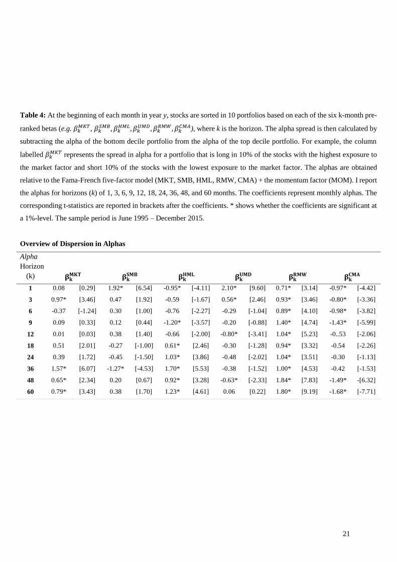
Table 4: Overview of Dispersion in Alphas ........................................................................................ 21

Table 5: Overview Dispersion in Alphas (incl. Illiquidity) ................................................................. 25

Table 6: Overview Dispersion in Alphas (incl. Opacity) .................................................................... 32

Table 7: Overview Results .................................................................................................................. 39

Table 8: Z-Statistics for Regressions With an Without Illiquidity ...................................................... 47

Table 9: Z-Statistics for Regressions With an Without Opacity ......................................................... 48

Table 10: Overview Illiquidity Levels at Different Horizons ............................................................. 49

Table 11: Overview Opacity Levels at Different Horizons ................................................................. 50

vii

LIST OF FIGURES

Figure 1: Overview of Dispersion in Excess Returns ........................................................................ 17

Figure 2: Overview of Dispersion in Alphas....................................................................................... 22

Figure 3: Overview Dispersion in Alphas (incl. Illiquidity) ............................................................... 26

Figure 4: Illiquidity – Market Factor ................................................................................................... 28

Figure 5: Illiquidity – Size Factor ....................................................................................................... 29

Figure 6: Illiquidity – Value Factor .................................................................................................... 29

Figure 7: Illiquidity – Momentum Factor ........................................................................................... 30

Figure 8: Illiquidity – Profitability Factor ........................................................................................... 30

Figure 9: Illiquidity – Investment Factor ............................................................................................ 31

Figure 10: Overview Dispersion in Alphas (incl. Opacity) ................................................................. 33

Figure 11: Opacity – Market Factor .................................................................................................... 34

Figure 12: Opacity – Size Factor ......................................................................................................... 35

Figure 13: Opacity – Value Factor ..................................................................................................... 35

Figure 14: Opacity – Momentum Factor ............................................................................................. 36

Figure 15: Opacity – Profitability Factor ............................................................................................ 36

Figure 16: Opacity – Investment Factor .............................................................................................. 37

1

CHAPTER 1: Introduction

There is a consensus among academics on the existence of certain macroeconomic variables that are

classified as systematic priced risk factors. Risk factors are defined as characteristics relating to a group

of securities that is important in explaining their return and risk. Such factors have historically earned a

risk premium and represent exposure to systematic sources of risk. However, a shortcoming in the vast

majority of prior academic research regarding systematic risk factors, is that they solely focuses on a

single-period analysis. Whereas, in practice different investors have various horizons. The importance

of incorporating various horizons in the research to the pricing of systematic risk factors is significant,

because recent literature showed that systematic risk factors can be priced differently over time.

1.1 Research question

This study will incorporate various horizons and tests whether there is dispersion in the pricing of

systematic risk factors over those horizons. In the study six equity systematic risk premia factors are

examined: market, value, size, momentum, profitability and investment. The abovementioned factors

will be priced at various horizons ranging from 1 month to 5 years (60 months). This study will be

performed by looking at data from the equity market in the People’s Republic of China (henceforth

mentioned as China). The main question that this study will try to answer is the following:

‘’Are there systematic risk factors that can explain the cross-sectional return at one horizon, where

it does not at another horizon?’’

If there is indeed dispersion in how systematic risk factors are priced over various horizons two control

variables will be introduced that might explain this dispersion. These control variables are illiquidity

and opaqueness (transparency).

1.2 Scientific Relevance

Until recently, most research of the pricing of systematic risk factors has been based on an one-period

horizon, neglecting other horizons. There is an upcoming stream of literature that does incorporate

different horizons in their study for the pricing of systematic risk factors (see e.g., Kamara, Korajczyk,

Lou, and Sadka, 2015; Gilbert, Hrdlicka, Kalodimos, and Siegel, 2014). However, horizon pricing is

still a relatively recent topic, wherein there is still a lot of room for additional research.

This study is - to my knowledge - the first to study multiple systematic risk factors over different

horizons in China. China is chosen as the reference country, because China is the biggest emerging

market, meaning a country that is in the process of rapid growth and development, with lower per capita

incomes, less mature capital markets and with a lower market liquidity relative to a developed market.

It might be interesting to see whether the results from this study differ from the results that are previously

found in developed markets. There are more distinctive characteristics that distinguish the Chinese stock

2

market from other countries (e.g. weak legal framework, heavy government involvement such as

regulation and central bank intervention, and a relatively high level of state owned enterprises). Demirer

& Kutan (2006) hypothesize that due to the abovementioned distinctive characteristics investors are

more likely to act like speculators and follow the market consensus. Therefore, traders in China tend to

behave more like positive feedback traders: they sell when prices fall and buy when prices rise. Another

distinctive characteristic of the Chinese stock market is the fact that the Chinese stock market is fuelled

by undereducated and inexperienced traders. New data from the China Household Finance Survey, a

large-scale survey of household income and assets headed by Professor Li Gan of Southwestern

University of Finance and Economics, shows that two thirds of new equity investors excited the

education system by middle school (Orlik, 2015). As a result of these distinctive characteristics, trading

behaviour in Chinese markets may differ significantly from other markets.

1.3 Social Relevance

Hence, besides the relevance of being the first study, outcomes of this study can be socially relevant as

well. For example, it can be used in the relative new approach of investing: factor investing. Factor

investing describes the investment process that aims to harvest risk premia through exposure to

systematic risk factors. Factor investing has become an investment strategy that is a more widely used

approach for various forms of financial institutions like hedge funds, mutual funds, pension funds etc.

Incorporating horizons to price risk factors can give important implications for the implementation of

the factor investing approach. Pension funds, for instance, are established to invest the employees’

retirement savings, and therefore expect to grow over the long term. Therefore, for pension funds it is

more likely to invest in systematic risk factors that are priced in the long run. The opposite would apply

for financial institutions such as hedge funds and mutual funds.

However, China lacks in the number of investors with long-term investment horizons, such as

pension funds, which may also explain the existence of so many speculators in China. If several

systematic risk factors appear to be priced over the longer term, increasing the participation of long-

term investors (e.g. experienced foreign pension funds, insurance companies, and long-term investment

funds in domestic markets) seems like a good way to make capital markets more efficient (Pettis, 2013).

China has already made their first steps towards increasing the participation of long-term investors by

implementing the Qualified Foreign Institutional Investor program, wherein China allows global

institutional investors, on a selective basis, to invest in its capital markets.

1.4 Preliminary results

Using a portfolio analysis, the results show that there is dispersion in how the six systematic risk factors

used in this study are priced at different horizons. This is done by obtaining the spread in excess returns

and alphas (relative to the Fama-French five-factor model + momentum) between the portfolio decile

wherein stocks have the most exposure to a particular factor and the portfolio decile wherein stocks have

3

the least exposure to a particular factor. The excess returns appear to be especially significant at relative

intermediate-term horizons for the market, value and profitability factors. However, despite the excess

returns being significant, they are also negative. This means that an intermediate horizon investor that

purely looks at generating excess returns, may consider a strategy wherein it takes a long position in

stocks with high exposure to the market/value/profitability factor and a short position in stocks with low

exposure to the market/value/profitability factor as unattractive. The size factor has significant positive

excess returns for all horizons, nevertheless, the short horizons are most significant. Therefore, the size

factor seems to be priced explicitly at short-term horizons. The momentum factor exhibits significant

excess returns for all horizons. Meanwhile, the investment factor has is just priced significantly and

positively over longer horizons.

When looking at alpha the market and value factors seem to be priced over relatively longer

horizons, implying the more significant coefficients at longer horizons. The alphas are positive at longer

horizons for the market and value factor. A long-term horizon investor that purely looks at beating the

benchmark (FF5-factor model + momentum) and generating alpha may consider a strategy where it

takes a long position in stocks with high exposure to the market/value factor and a short position in

stocks with low exposure to the market/value factor as attractive. The size factor has significant alphas

over the 1 month and 36 months horizons, it is therefore hard to draw a conclusion on what term the

size factor is priced. The same applies to the momentum factor that has significant alphas for the 1, 3,

12, and 48 months horizons. However, with the 1 and 3 months horizon being priced it seems that the

momentum factor is priced at short-term horizons. The profitability factor has positive alphas for all

horizons. The investment factor has significant alphas for short and long-term horizons. Therefore, the

investment factor is priced at short and long-term horizons, however not for intermediate horizons.

With the aim to explain the dispersion in returns over various horizons two control variables are

added. The first is illiquidity measured by the Amihud illiquidity measure (2002), the second is opacity

measured by the variance in discretionary accruals. Both control variables have no significant impact in

the explanation of the dispersion in the pricing of the systematic risk factors over various horizons.

1.5 Outline of the paper

The remainder of the paper is organized as follows. Chapter 2 provides a literature review in which the

risk factors are introduced and the pricing of the systematic risk factors over different horizons are

discussed in an academic context. Chapter 3 describes the data-gathering process, provides information

how respectively the factors and betas are constructed, and introduces the proxies for the control

variables. Chapter 4 discusses the results. It looks for each individual systematic risk factor whether

there is dispersion in the pricing over various horizons, and whether this dispersion can be explained by

two control variables: illiquidity and opacity. Chapter 5 will give a brief summary of the results and

discusses the limitations of this paper and provides possible directions for future research.

4

CHAPTER 2: Literature Review

2.1 Introduction of Risk Factors

The mean-variance portfolio theory developed by Markowitz (1952, 1959) has been considered as the

cornerstone for the many asset pricing models that are known nowadays. The mean-variance portfolio

theory of Markowitz states that investors select a portfolio at t-1 that produces a random return at t. In

the model it is assumed that investors are risk averse, that investors maximize one-period expected

utility, and that investors care only about the expected return and the variance of return, where the

expected return is desirable and variance of return an undesirable.

The Capital Asset Pricing Model (henceforth mentioned as CAPM) of Sharpe (1964), Lintner

(1965), and Black (1972) builds on the mean-variance portfolio theory, and is considered as the first

asset pricing model with clear testable predictions about risk and return (Fama & French, 2004). The

central prediction of the CAPM is that the market portfolio of invested wealth is mean-variance efficient

in the sense of Markowitz (1952, 1959). The efficiency of the market portfolio implies that (i) expected

returns on securities are a positive linear function of their market betas (the slope in the regression of a

security’s return on the market’s return), and (ii) market betas suffice to describe the cross-section of

expected returns (Fama & French, 1992). Hence, with the market factor (MKT) the CAPM introduced

the first systematic risk factor that tried to capture the excess returns of securities.

Many authors criticized the CAPM, by arguing that the cross-section of average returns on

stocks showed little relation to the market betas (see e.g., Reinganum, 1981; Breeden, Gibbons, and

Litzenberger, 1989). Therefore, several other macroeconomic variables have been proposed in the asset

pricing literature as systematic priced risk factors.

The first extension on the CAPM model came from the work of Fama & French (1993), who

have proposed a three-factor model. The model says that expected return on a portfolio in excess of the

risk free rate is not just explained by the market factor (i.e. the excess return on a broad market portfolio),

the expected return is as well explained by the sensitivity of its return to two other factors: (i) size, the

difference between the return on a portfolio of small stocks and the return of a portfolio of large stocks

(SMB, small minus big); and (ii) value, the difference between the return on a portfolio of high-book-

to-market stocks and the return on a portfolio of low-book-to-market stocks (HML, high minus low).

In reaction to the three-factor model proposed by Fama and French (1993), Carhart (1997)

stresses the three-factor model inability to explain cross-sectional variation in momentum-sorted

portfolio returns. Therefore, he constructs a four-factor model using Fama and French three-factor model

plus an additional factor capturing Jegadeesh and Titman’s (1993) one-year momentum anomaly. This

momentum factor is the difference between the return on a portfolio of stocks that have performed well

over the prior year and the return on a portfolio of stocks that performed poorly over the prior year.

Besides Carhart (1997) there was more criticism regarding the three-factor model of Fama &

French (1993). For example, Novy-Marx (2013), Titman, Wei, and Xie (2004), and others state that the

5

three-factor model is an incomplete model for expected returns, because the three factors miss much of

the variation in average returns related to profitability and investment. Therefore, Fama & French (2015)

add profitability and investment to the three-factor model. The profitability factor displays the difference

between returns on diversified portfolios of stocks with robust and weak profitability (RMW), and the

investment factor displays the difference between returns on diversified portfolios of the stocks of low

and high investment firms, which the authors call conservative and aggressive (CMA).

2.2 Incorporating Horizons

In single-period models, like the CAPM, it is assumed that investors do only care about the mean and

variance of their one-period investment return. The theory remains silent about the investment horizons

of investors. Where, in practice, investors have different investment horizons. For instance, leveraged

quantitative hedge funds are more likely to have short investment horizons in order to reap benefits to

deliver returns from arbitrage opportunities, compared to pension funds, who are emerged in more

responsible investment strategies to generate stable growth on the long term. However, it is not just the

CAPM that remains silent about the investment horizons, in by far the majority of the asset pricing tests

the horizon is taken as one month and returns are measured over monthly intervals (Brennan, and Zheng,

2012). This while the difference in investment horizons across different investors or investment

institutions is of significant importance, because there could be a change in risk dynamics across

different horizons.

A recent stream of literature stress the importance of incorporating different horizons in their

research to examine the risk of risk factors. Kamara, Korajczyk, Lou, and Sadka (2015), for example,

examine whether systematic risk factors can explain the differences in cross-sectional returns for one

horizon while the risk measured over another horizon does not. The authors find that the liquidity risk

factor seems to capture a short-horizon risk, implying that liquidity risk is priced on the short term.

However, at longer horizons the risk premium of the liquidity beta falls substantially to insignificant

levels. In contrast, the market, and the value factors seem to behave like intermediate-horizon systematic

risk factors. Market risk is priced at the 6 and the 12 months horizon, while the value factor is priced at

the 2 year and 3 year horizon. For the momentum and the size risk factors no significant values are found

by the authors, from which they insinuate that both risk factors are not able to explain excess returns for

any of their formulated horizons.

Gilbert, Hrdlicka, Kalodimos, and Siegel (2014) test whether the CAPM is able to explain the

differences in cross-sectional returns. They use both daily and quarterly return data over the previous

five years to estimate lagged CAPM-betas. They then sort stocks into five quantile portfolios based on

the difference between daily and quarterly CAPM-betas. The alphas are than estimated by going long

in portfolio 5 and short in portfolio 1. It appears that at the daily frequency, the alphas (i.e. the pricing

error relative to the CAPM) for almost all portfolios are positive and significantly different from zero

(except for the top decile portfolio which is insignificant). At the quarterly frequency, the alphas are

6

insignificant and generally lower relative to the daily frequency. This translates in a significant

difference in the alphas between daily and quarterly frequencies. The results tell that CAPM can explain

excess returns at the quarterly frequency, due to its insignificant alphas. However, at the daily frequency

the CAPM cannot fully explain excess returns and the market factor seems to outperform the CAPM

benchmark. This suggest that at daily frequency, taking exposure to the market factor delivers a higher

alpha and is therefore positively priced. Short-term investors can reap benefits from investment

strategies wherein it takes a long position in high exposure to the market factor.

Boons and Tamoni (2016) highlight the importance to account for horizon-specific exposures

to macroeconomic risk when connecting the prices to the real economy. The authors’ test at which

horizon macroeconomic growth and volatility risk provide the strongest determination of asset returns.

Boons and Tamoni show that long-term risk, measured as the covariance between four year returns with

innovations in economic growth and volatility with matching half-life (i.e. the authors scale the returns

based on how far in the past this returns occurred, for each day/month the returns get weighted by a

multiplier of a number less than 1. The half-life is the sum of all past returns divided by the sum of the

weights, which gives a weighted average of the past returns), is priced. Whereas, short-term risk appears

not to be priced. Therewith, the results in their study strongly support using long-horizon betas to

measure systematic risks in asset returns.

Kang et al. (2002) examine the behaviour of stock returns in the Chinese stock market. They try

to find momentum (i.e. past winners are bought and past losers are shorted) profits and contrarian

momentum (i.e. past losers are bought and past winners are shorted) profits at different holding periods.

The authors find statistically significant profits for the momentum strategy at the intermediate-term

horizon and statistically significant profits for the contrarian momentum strategy at the short-term

horizon. The contrarian momentum profits appear more distinct, the authors explain this due to the

dominance of overreaction to firm-specific information. This excessive overreaction can be attributed

due to the dominance of individual investors in the Chinese stock market, the lack of reliable information

on firms, and the dominance of speculators in the Chinese stock market who favour to create a bullish

sentiment on small stocks.

2.3 Control Variables

The studies of Kamara et al. (2015), Gilbert et al. (2014), Boons and Tamoni (2016), and Kang et al.

(2002) infer coinciding results regarding their findings that systematic risk factors are priced differently

over various horizons. For example, Kamara et al. find that market and value factor are just priced at

intermediate horizons, where the liquidity factor is priced at the short-term horizon. The existing

literature provides us with explanations why there is dispersion in the way various horizons are priced.

7

2.3.1 Opacity

One often mentioned explanation is the opaqueness of firms. Gilbert et al. (2014) pose that additional

risk arises because the systematic news of opaque firms is revealed with a delay. In a situation where an

opaque firm receives better than expected systematic news, opaque firms have higher risk and hence

higher expected returns. However, due to the delay in the revealing of the better than expected systematic

news, the short-term realized returns are lower than the expected returns. In contrast, for transparent

firms the revelation of the impact of systematic news is immediate. Therefore, the riskiness and expected

returns does not vary from realized returns with either good or bad systematic news. Transparent firms

generally make up for most of the market, the realized returns of opaque firms co-move less with the

market on shorter term horizons, and the opposite being true for realized returns of transparent firms,

that co-move more with the market on shorter term horizons. This dampens the betas for opaque firms

and enlarges the betas for transparent firms at shorter horizons. These differences in betas are expected

to lead to differences in alphas. For example, when the market is going down alphas are positive for

opaque firms and negative for transparent firms at short horizons and zero for both transparent and

opaque firms at the longer term horizons.

The opacity effect is expected to be especially pronounced in the Chinese stock market, since

one of the biggest problems in China facing investors is the transparency of Chinese stocks. Reporting

requirements for listed Chinese companies are neither well developed and less comprehensive in

comparison to the stock markets of more developed countries (Demirer & Kutan, 2006).

2.3.2 Illiquidity

Amihud and Mendelson (1986) provide an explanation based on liquidity. They model a market where

rational traders differ in their expected holding periods and where assets have different bid-ask spreads.

Their equilibrium has the following characteristics: (i) market-observed average returns are an

increasing function of the spread; (ii) the asset return of equity holders, net of trading costs, increase

with a higher bid-ask spread (due to investors demanding a higher liquidity premium); (iii) there is a

clientele effect, whereby stocks with higher spreads are held by investors with longer holding periods;

and (iv) due to the clientele effect, returns on higher-spread stocks are less spread-sensitive. The model

of Amihud and Mendelson (1986) implies that the dispersion between short-term and long-term risk

could be due to liquidity.

Illiquidity is expected to be especially pronounced in the Chinese stock market, because the

Chinese stock market is dominated by positive feedback traders. When positive feedback traders

dominate the market, market prices are liable to be unstable and the market may become one-sided and

illiquid. A reduction in the price of an asset causes the trader to sell. This results in prices falling further

and more selling. The opposite applies when asset prices increase which causes traders to buy. This

results in the price of the asset increasing further and more buying (Hull, 2015).

In Table 1 there is an overview of the literature that is most relevant for this research.

8

Table 1: This table contains a literature table, which gives a brief summarization of all the main

findings that are relevant for the research.

Literature Table

Authors Region Time period Result

Fama and French

(1992)

United

States

1962 - 1989 Significant evidence that size and value factors

explain cross-sectional variation in excess returns.

Jegadeesh and Titman

(1993)

United

States

1965 - 1989 Strategy of buying stocks that performed well in the

past and sell stocks that performed poorly, is a

profitable strategy that are not due to their systematic

risk or to delayed stock price reactions to common

factors.

Carhart

(1997)

United

States

1962 - 1993 Consistent with Jegadeesh and Titman (1993),

Carhart also found that momentum strategies are

profitable, and he added the momentum factor to the

existing three-factor model of Fama and French

(1992).

Fama and French

(2015)

United

States

1963 - 2013 Finds that adding profitability and investment

factors leads to a better performing model in

capturing the cross-sectional variation in excess

returns.

Kamara, Korajczyk, Lou,

and Sadka

(2015)

United

States

1962 – 2013 Finds that the liquidity, market, value, size and

momentum factors are priced differently over

different time horizons.

Boons and Tamoni

(2016)

United

States

1962 - 2011 The results favour using long-horizon betas to

measure macroeconomic risk in asset returns.

Gilbert, Hrdlicka,

Kalodimos, and Siegel

(2014)

United

States

1969 - 2010 Shows that CAPM works better at longer horizons,

and therefore for low-frequency traders. The results

also indicate that the dispersion of beta can be

explained by the opaqueness or transparency of a

firm.

Amihud and Mendelson

(1986)

United

States

1960 – 1979 Their model implies that the difference in risks for

short and long-term horizons can be explained by

liquidity.

9

CHAPTER 3: Data & Methodology

3.1 Sample and criteria

The sample consists of Chinese companies listed on the two main stock exchanges in China: the

Shanghai Stock Exchange and the Shenzhen Stock Exchange, and a minority of Chinese firms listed on

three stock exchanges outside China: the Hong Kong Stock Exchange, the Singapore Stock Exchange

and the Taiwan Stock Exchange. The firms’ fundamentals are collected from Compustat Global

Fundamentals Annual. The monthly stock prices, the risk free rate, turnover per value, and the index

constituents are obtained from Datastream (see Appendix A for description of all variables used). The

sample runs from June 1995 to December 2015. The proxy for the risk free rate is the China 3-months’

time deposit rate, it was difficult to find a proxy with a time series of length that did stroke with the

period investigated, the China 3-months’ time deposit therefore seemed the best fit to satisfy this

condition.

To overcome issues with the data several criteria were applied. Firstly, penny stocks (i.e. stocks

with a price below 1 Yuan) were excluded. This is because, penny stocks are mostly neglected by

financial institutions. Due to their low price, penny stocks have a high price sensitivity to the level of

trading, which makes them highly speculative. Secondly, also the fundamentals that were reported in

another currency than the Chinese Yuan, which is the main currency for China, were excluded. After

these criteria were applied the final dataset contains of 3045 firms.

3.2 Returns

The monthly stock prices for the Chinese firms and the risk free rate can be used for calculating the

monthly excess returns. This can be done by using the following formula:

𝑅𝑖,𝑡 = 𝑝𝑖,𝑡− 𝑝𝑖,𝑡−1

𝑝𝑖,𝑡−1− 𝑟𝑓𝑖,𝑡,

Where 𝑅𝑖,𝑡 is the excess return for firm i at time t, 𝑝𝑖,𝑡 is the closing price of firm i at time t adjusted for

dividends, 𝑝𝑖,𝑡−1 is the closing price of firm i at time t-1 adjusted for dividends, and 𝑟𝑓𝑖,𝑡 is the risk free

rate of firm i at time t. The excess returns will be used in creating the market, size, value, momentum,

profitability, and investment factors.

3.3 Creating Factors

To create the abovementioned factors the methods described on the website of Ken French1 were

followed. The explanations how to define and calculate the factors are also employed in Fama & French

(1992, 2015). The fundamentals and monthly prices are used to define the variables that later will be

1 I thank Ken French, for the extensive description of the variables, and how the factors are formed.

http://mba.tuck.dartmouth.edu/pages/faculty/ken.french/data_library.html

10

used to construct the factors. The market equity is the monthly price times the number of shares

outstanding. The book equity is the book value of stockholders’ equity plus balance sheet deferred taxes

and investment tax credit. With the market and book value defined, it is possible to define the book-to-

market ratio, which is the book value for the fiscal year ending in calendar year t-1, divided by market

equity at the end of December of t-1. The operating profitability ratio is defined as the annual revenues

minus the cost of goods sold interest expense, and the selling, general, and administrative expenses

divided by book equity for the last fiscal year end in t-1. The investment ratio is the change in assets

from the fiscal year ending in year t-2 to the fiscal year ending in year t-1.

At the end of June for each year, stocks are sorted and allocated to their respective portfolios

This allocation is done based on four variables, respectively market equity (size), market-to-book ratio

(value), operating profitability ratio (profitability) and investment ratio (investment). In contrast, the

allocation based on momentum is done for each month of each year. To obtain the factors Fama &

French use a double sorting approach.

The size factor (SMB – small minus big) is constructed by first use two value-weighted

portfolios on size (i.e. split the sample in the 50% stocks of the smallest companies and the 50% stocks

of the biggest companies), and use three value-weighted portfolios over the two size portfolios formed

on the book-to-market ratio. Which provides six (2x3) value-weighted portfolios formed on size and

book-to-market:

𝑆𝑀𝐵(𝐵/𝑀) = 13⁄ ∗ (𝑆𝑚𝑎𝑙𝑙 𝑉𝑎𝑙𝑢𝑒 + 𝑆𝑚𝑎𝑙𝑙 𝑁𝑒𝑢𝑡𝑟𝑎𝑙 + 𝑆𝑚𝑎𝑙𝑙 𝐺𝑟𝑜𝑤𝑡ℎ)

− 13⁄ ∗ (𝐵𝑖𝑔 𝑉𝑎𝑙𝑢𝑒 + 𝐵𝑖𝑔 𝑁𝑒𝑢𝑡𝑟𝑎𝑙 + 𝐵𝑖𝑔 𝐺𝑟𝑜𝑤𝑡ℎ)

After, the double sorting approach is also used to create six value-weighted portfolios formed on size

and momentum, size and profitability, and size and investment.

𝑆𝑀𝐵(𝑀𝑂𝑀) = 13⁄ ∗ (𝑆𝑚𝑎𝑙𝑙 𝑈𝑝 + 𝑆𝑚𝑎𝑙𝑙 𝑀𝑒𝑑𝑖𝑢𝑚 + 𝑆𝑚𝑎𝑙𝑙 𝐷𝑜𝑤𝑛)

− 13⁄ ∗ (𝐵𝑖𝑔 𝑈𝑝 + 𝐵𝑖𝑔 𝑀𝑒𝑑𝑖𝑢𝑚 + 𝐵𝑖𝑔 𝐷𝑜𝑤𝑛)

𝑆𝑀𝐵(𝑂𝑃) = 13⁄ ∗ (𝑆𝑚𝑎𝑙𝑙 𝑅𝑜𝑏𝑢𝑠𝑡 + 𝑆𝑚𝑎𝑙𝑙 𝑁𝑒𝑢𝑡𝑟𝑎𝑙 + 𝑆𝑚𝑎𝑙𝑙 𝑊𝑒𝑎𝑘)

− 13⁄ ∗ (𝐵𝑖𝑔 𝑅𝑜𝑏𝑢𝑠𝑡 + 𝐵𝑖𝑔 𝑁𝑒𝑢𝑡𝑟𝑎𝑙 + 𝐵𝑖𝑔 𝑊𝑒𝑎𝑘)

𝑆𝑀𝐵(𝐵/𝑀) = 13⁄ ∗ (𝑆𝑚𝑎𝑙𝑙 𝐶𝑜𝑛𝑠𝑒𝑟𝑣𝑎𝑡𝑖𝑣𝑒 + 𝑆𝑚𝑎𝑙𝑙 𝑁𝑒𝑢𝑡𝑟𝑎𝑙 + 𝑆𝑚𝑎𝑙𝑙 𝐴𝑔𝑔𝑟𝑒𝑠𝑠𝑖𝑣𝑒)

− 13⁄ ∗ (𝐵𝑖𝑔 𝐶𝑜𝑛𝑠𝑒𝑟𝑣𝑎𝑡𝑖𝑣𝑒 + 𝐵𝑖𝑔 𝑁𝑒𝑢𝑡𝑟𝑎𝑙 + 𝐵𝑖𝑔 𝐴𝑔𝑔𝑟𝑒𝑠𝑠𝑖𝑣𝑒)

The size factor is then simply obtained by taking the average return of the twelve small stock portfolios

(e.g. small value, small neutral, small growth, small robust, etc.) minus the average return of the twelve

big stock portfolios (e.g. big value, big neutral, big growth, big robust, etc.).

11

𝑆𝑀𝐵 = 14⁄ ∗ (𝑆𝑀𝐵(𝐵/𝑀) + 𝑆𝑀𝐵(𝑀𝑂𝑀) + 𝑆𝑀𝐵(𝑂𝑃) + 𝑆𝑀𝐵(𝐵/𝑀))

A similar way is used to calculate the value factor (HML – high minus low), the profitability factor

(RMW – robust minus weak) and the investment factor (CMA – conservative minus aggressive). The

six value-weighted portfolios formed on size and book-to-market, size and profitability, and size and

investment were calculated to create the three abovementioned systematic risk factors.

𝐻𝑀𝐿 = 12⁄ ∗ (𝑆𝑚𝑎𝑙𝑙 𝑉𝑎𝑙𝑢𝑒 + 𝐵𝑖𝑔 𝑉𝑎𝑙𝑢𝑒)

− 12⁄ ∗ (𝑆𝑚𝑎𝑙𝑙 𝐺𝑟𝑜𝑤𝑡ℎ + 𝐵𝑖𝑔 𝐺𝑟𝑜𝑤𝑡ℎ)

𝑅𝑀𝑊 = 12⁄ ∗ (𝑆𝑚𝑎𝑙𝑙 𝑅𝑜𝑏𝑢𝑠𝑡 + 𝐵𝑖𝑔 𝑅𝑜𝑏𝑢𝑠𝑡)

− 12⁄ ∗ (𝑆𝑚𝑎𝑙𝑙 𝑊𝑒𝑎𝑘 + 𝐵𝑖𝑔 𝑊𝑒𝑎𝑘)

𝐶𝑀𝐴 = 12⁄ ∗ (𝑆𝑚𝑎𝑙𝑙 𝐶𝑜𝑛𝑠𝑒𝑟𝑣𝑎𝑡𝑖𝑣𝑒 + 𝐵𝑖𝑔 𝐶𝑜𝑛𝑠𝑒𝑟𝑣𝑎𝑡𝑖𝑣𝑒)

− 12⁄ ∗ (𝑆𝑚𝑎𝑙𝑙 𝐴𝑔𝑔𝑟𝑒𝑠𝑠𝑖𝑣𝑒 + 𝐵𝑖𝑔 𝐴𝑔𝑔𝑟𝑒𝑠𝑠𝑖𝑣𝑒)

In determining the value, profitability and investment factors, the neutral portfolios are neglected. The

value factor is obtained by taking the average return of two value portfolios minus the average return on

two growth portfolios. Similarly, the profitability and investment factors are determined by taking the

average return of two robust/conservative portfolios minus the average return on two weak/aggressive

portfolios. Momentum is defined as the return of a company over the prior 12 months excluding the

most recent month. To construct the momentum factor, six-value weighted portfolios are formed on size

and momentum. The neutral portfolios are again neglected, and the momentum factor is constructed by

taking the average return on two highest momentum portfolios minus the average return on two low

momentum portfolios.

𝑈𝑀𝐷 = 12⁄ ∗ (𝑆𝑚𝑎𝑙𝑙 𝑈𝑝 + 𝐵𝑖𝑔 𝑈𝑝)

− 12⁄ ∗ (𝑆𝑚𝑎𝑙𝑙 𝐷𝑜𝑤𝑛 + 𝐵𝑖𝑔 𝐷𝑜𝑤𝑛)

The construction of the market factor is somewhat more intuitive. It is simply the difference between

the percentage change in the market index from the stock exchange where the company is listed minus

the risk free rate. Since in the sample companies are listed on five different stock exchanges, there are

also five market indices used to determine the market factor.

3.4 Horizon factors

The monthly factors can be used to determine factors of horizon k. The method to construct factors of

horizon k is similar to Kamara et al. (2015). First it is important to note that each of the factors represent

an excess return portfolio. For example, the market factor is the excess return of the market index over

12

the risk free rate and the size factor is the excess return of a small company portfolio over a big company

portfolio. Similarly, the k-month factors are the excess return in the k-period of a long portfolio over a

short portfolio. For example the size factor of horizon k is the k-period return of small company

portfolios minus the k-period return of big company portfolios. This can be denoted with the following

formula:

𝑓𝑘,𝑡𝑆𝑀𝐵 = ∏ (1 + 𝑟1,𝑡−𝑘

𝑠𝑘−1𝑘=0 ) - ∏ (1 + 𝑟1,𝑡−𝑘

𝑏𝑘−1𝑘=0 ) ,

where 𝑘1,𝑡𝑠 is the monthly return for the small company portfolio at time t, and 𝑘1,𝑡

𝑏 is the monthly return

for the big portfolio company at time t. The formula will be applied to calculate the size factors for the

1, 3, 6, 9, 12, 18, 24, 36, 48, 60 months horizons. Note that the same formula can be used for determining

the other systematic risk factors at various horizons as well.

3.5 Betas

After the factors are obtained for different horizons, portfolios are formed based on pre-ranked betas for

the six systematic risk factors at the end of each month for each firm. Betas are estimated for various

horizons by using overlapping k-months returns and factors in the five years prior to the portfolio-

formation month. The beta estimation requires at least 24 observations for both the factors and the

returns. For example, the beta of the market factor is calculated as follows:

𝛽𝑘𝑀𝐾𝑇 =

𝐶𝑜𝑣 (𝑟𝑘,𝑡𝑒 , 𝑓𝑘,𝑡

𝑀𝐾𝑇)

𝑉𝑎𝑟(𝑓𝑘,𝑡𝑀𝐾𝑇)

The pre-ranked betas will be used in an portfolio analysis, where the pricing of a factor at a particular

horizon will be derived by taking a long position in the top decile portfolio, and a short position in the

bottom decile portfolio. The top decile portfolio represents the 10% of stocks with the biggest exposure

to a particular factor, meaning the 10% stocks which returns co-move most with the factor. The bottom

decile portfolio represents the 10% of stocks with the lowest exposure to a particular factor, meaning

the 10% stocks which returns co-move least with the factor.

3.6 Illiquidity

Two control variables are introduced that might explain why dispersion in the pricing of the factors at

various horizons can be observed. The first control variable is illiquidity. However, illiquidity is an

elusive concept, and cannot be observed directly. Therefore, a proxy needs to be found that does well in

capturing illiquidity. Numerous of proxies for illiquidity have been proposed in the literature. The most

used proxy is Amihud’s illiquidity measure (Amihud, 2002), which is defined as the average ratio of the

daily absolute return to the dollar trading volume on that day. The Amihud illiquidity measure has two

13

main advantages over other measures: 1) the Amihud illiquidity measure has a simple construction and

it relies on the wide availability of data for its computation; 2) the measure has a strong positive relation

to expected stock return. The Amihud illiquidity measure can be defined as follows:

𝐼𝐿𝐿𝐼𝑄𝑖𝑦 = 1/𝐷𝑖𝑦 ∑ |𝑅𝑖𝑦𝑑| /𝑉𝑂𝐿𝑖𝑦𝑑𝐷𝑖𝑦

𝑡=1 ,

where 1/𝐷𝑖𝑦 is the number of days for which data was available for stock i in year y, |𝑅𝑖𝑦𝑑| is the return

on stock i on day d, and 𝑉𝑂𝐿𝑖𝑦𝑑 is the respective daily volume in dollars. However, since monthly

returns are used in the sample of this study, the Amihud illiquidity measure can be rewritten in such a

way that it can applied it on the data.

𝐼𝐿𝐿𝐼𝑄𝑖𝑦 = 1/𝑀𝑖𝑦 ∑ |𝑅𝑖𝑦𝑚| /𝑉𝑂𝐿𝑖𝑦𝑚𝑀𝑖𝑦

𝑡=1 ,

where 1/𝑀𝑖𝑦 is the number of months for which data was available for stock i in year y, |𝑅𝑖𝑦𝑚| is the

return on stock i in month m, and 𝑉𝑂𝐿𝑖𝑦𝑚 is the respective monthly volume in Yuan (Chinese currency).

3.7 Opacity

The other control variable is opacity, or the transparency of financial disclosure of a firm. Same as

illiquidity, also opacity is a difficult variable to grasp. Gilbert et al. (2014) try to explain dispersion in

the pricing of the CAPM (market factor) at daily return data and quarterly return data by looking to

opacity as well. One of the measures they use to proxy opacity is the variance in discretionary (abnormal)

accruals. Discretionary accruals are non-mandatory expenses/assets which are recorded within the

accounting system but still need to be realized. According to Healy (1996), discretionary accruals are

the accruals that can be influenced by the management. So for example, a manager can influence

earnings by choosing a general accepted procedure defined by accounting standard-setting bodies, that

maximizes the earning for that particular year. So discretionary accruals can be used by managers to

manipulate earnings. High discretionary accruals indicate that managers manipulate accruals in such a

way that the earnings in the accounting year are higher than the actual earnings, and low discretionary

accruals indicate that managers manipulate accruals in such a way that earnings in the accounting year

are lower than the actual earnings. Manipulating accruals so that earnings are lower than the actual

earnings is done to carry the earnings over to the following years. The question that remains is, how

does the variance of discretionary accruals relate to the opaqueness of a firm. Gilbert et al. (2014) explain

that the more managers make use of accruals to manage the firms’ earnings, the harder it will be for

investors to understand the impact of systematic news on the value of the firm. A firm that has a high

variance of discretionary accruals is more opaque in the sense that investors require more information

14

and hence more time to price the impact of news because, the production function is more difficult to

discern.

In the academic literature there is a variety of models that try to measure discretionary accruals.

The models that will be briefly discussed are: the Healy model, the DeAngelo model, the Jones models,

and the modified-Jones model. These models are discussed in an attempt to give a better understanding

of why a particular model that measures discretionary accruals is chosen in this study. The Healy model

(1985) does measure non-discretionary accruals (note: the difference between accruals and non-

discretionary accruals are the discretionary accruals), by comparing the mean of total accruals scaled by

lagged total assets. In the Healy model the non-discretionary accruals follow a mean-reverting process.

The DeAngelo model (1986) differs from the Healy model, in that it uses the total accruals of the

previous period to estimate non-discretionary accruals, and in that the non-discretionary accruals follow

a random process. The Jones model (1991) relaxes the assumption that was made in the models of Healy

and DeAngelo, and states that non-discretionary accruals are constant. The Jones model attempts to

control the non-discretionary accruals for a changing economic environment. Also, the Jones Model

assumes that revenues are non-discretionary, which implies that the Jones model removes a part of the

discretionary accruals, or the accruals that can be managed. Dechow et al. (1995) did make a

modification to the Jones model by correcting the Jones model for the error when measuring

discretionary accruals for when discretion is exercised over revenue recognition, this model is known

as the modified-Jones model. To determine the discretionary accruals in this paper, the modified-Jones

model will be used. The advantages of the modified-Jones model is that it is easy to implement, and a

lot of variables are used to determine the discretionary accruals. The discretionary accruals according to

the modified-Jones model are calculated by obtaining the regression residuals of the following

regression:

𝑇𝐴𝑖𝑡 = 𝛼0 + 𝛼1(1 𝐴𝑠𝑠𝑒𝑡𝑠 𝑖𝑡−1⁄ ) + 𝛼2 (∆𝑅𝐸𝑉 − ∆𝑅𝐸𝐶)𝑖𝑡 + 𝛼3𝑃𝑃𝐸𝑖𝑡 + ∈𝑖𝑡,

where 𝑇𝐴𝑖𝑡 are the total accruals of firm i at time t, 𝐴𝑠𝑠𝑒𝑡𝑠 𝑖𝑡−1 are the assets of firm i from the previous

period, (∆𝑅𝐸𝑉 − ∆𝑅𝐸𝐶)𝑖𝑡 is the difference in the change of revenues and the change of receivables of

firm i at time t. and 𝑃𝑃𝐸𝑖𝑡 is the gross property, plant and equipment of firm i at time t. The regression

is performed by industry. After the discretionary accruals are computed, the variance of the discretionary

accruals is taken for each firm in the sample.

15

CHAPTER 4: Results

In this section I will discuss the results and try to determine whether risk factors are priced differently

over various horizons. However, to get a better overview of the data it is relevant to first look at the

descriptive statistics of the sample used in this study.

Table 2 reports that on average a Chinese firm has a monthly excess return of 1.73% over the

period of June 1995 to December 2015. Over the same period China experienced huge economic and

industrial growth, and also the stock markets in China grew enormously. This lead to the excess returns

being positive on average for Chinese firms. Table 2 also reports the average levels of illiquidity and

the variance of discretionary levels, so that the levels of illiquidity and the variance of discretionary

accruals at the different deciles, that will be reported in a later stage of the paper, are comparable.

Table 2: This table shows the average levels of the monthly excess returns, illiquidity and the variance

in discretionary accruals over the entire sample of 3045 Chinese firms. The sample period is June 1995

– December 2015.

Descriptive Statistics

Variable Mean Standard Deviation

Excess Return 1.73% 15.56%

Illiquidity 0.4343 0.8762

Variance of Discretionary Accruals 0.0070 0.0084

4.1 Dispersion in Excess Returns

Table 3 displays the dispersion in excess returns for six systematic risk factors. The coefficients

represent the monthly excess return on a portfolio that goes long in the 10% stock portfolio with the

highest exposure over n-months to a particular risk factor, and goes short in the 10% stock portfolio

with the lowest exposure over n-months to a particular risk factor. This is done to create an equity market

neutral position. So for example the coefficient of the market factor at 12 months (β12MKT) is -2.99. This

means that a strategy wherein a long position is taken in a portfolio that represent the 10% stocks with

the highest exposure to the market factor over the last 12 months, and a short position is taken in a

portfolio that represent the 10% stocks with the lowest exposure to the market factor over the last 12

months, does deliver an excess return of -2.99%. I will discuss how the systematic risk factors are priced

at different horizons by looking at each systematic risk factor individually.

4.1.1 Market Factor

Table 3 shows that the market factor exhibits an insignificant negative excess return at the 1 month

horizon. At the 3, 6, 9, and 12 months horizons the excess return level gradually decreases and excess

16

Table 3: At the beginning of each month in year y, stocks are sorted in 10 portfolios based on each of the six k-month pre-

ranked betas (e.g. 𝛽𝑘𝑀𝐾𝑇, 𝛽𝑘

𝑆𝑀𝐵, 𝛽𝑘𝐻𝑀𝐿 , 𝛽𝑘

𝑈𝑀𝐷, 𝛽𝑘𝑅𝑀𝑊, 𝛽𝑘

𝐶𝑀𝐴), where k is the horizon. The return spread is then calculated by

subtracting the excess return of the bottom decile portfolio from the excess return of the top decile portfolio. For example,

the column labelled 𝛽𝑘𝑀𝐾𝑇 represents the spread in excess returns for a portfolio that is long in 10% of the stocks with the

highest exposure to the market factor and short 10% of the stocks with the lowest exposure to the market factor. I report

the excess returns for horizons (k) of 1, 3, 6, 9, 12, 18, 24, 36, 48, and 60 months. The coefficients represent monthly

excess returns. The corresponding t-statistics are reported in brackets after the coefficients. * shows whether the

coefficients are significant at a 1%-level. The sample period is June 1995 – December 2015.

Overview of Dispersion in Excess Returns

Excess Return

Horizon

(k) 𝛃𝐤𝐌𝐊𝐓 𝛃𝐤

𝐒𝐌𝐁 𝛃𝐤𝐇𝐌𝐋 𝛃𝐤

𝐔𝐌𝐃 𝛃𝐤𝐑𝐌𝐖 𝛃𝐤

𝐂𝐌𝐀

1 -0.51 [-1.83] 3.83* [8.06] -0.21 [-0.81] -1.16* [-3.58] -0.28 [-0.93] -0.21 [-0.80]

3 -1.99* [-5.43] 4.65* [10.20] -2.92* [-6.02] -2.48* [-6.75] -0.52 [-1.63] -0.29 [-0.99]

6 -3.26* [-8.25] 4.71* [10.48] -2.93* [-6.69] -2.55* [-6.47] 0.09 [0.34] -0.10 [-0.35]

9 -2.56* [-7.55] 4.29* [10.52] -3.66* [-8.47] -1.12* [-4.12] 0.19 [0.59] -0.07 [-0.28]

12 -2.99* [-8.16] 3.44* [9.28] -4.03* [-9.19] -1.56* [-5.50] -0.32 [-1.37] 0.62 [1.94]

18 -2.60* [-7.78] 2.83* [7.83] -2.89* [-8.42] -1.55* [-5.57] -1.07* [-3.59] 1.28* [4.14]

24 -1.90* [-6.31] 3.00* [7.96] -3.16* [-8.32] -1.83* [-6.41] -1.04* [-3.29] 0.99* [3.11]

36 -1.95* [-5.69] 2.92* [7.67] -2.51* [-6.30] -2.52* [-8.06] -0.76* [-2.76] 0.87* [2.69]

48 -1.54* [-3.94] 2.79* [6.64] -3.33* [-7.77] -3.06* [-8.83] 0.04 [0.18] 1.18* [4.17]

60 -0.36 [-1.26] 1.26* [4.38] -1.24* [-3.62] -2.57* [-8.07] 0.39 [1.92] 0.60* [2.40]

17

Figure 1: This figure summarizes Table 3, and give a graphical depiction of the excess return at each

horizon for each systematic risk factor. The y-axis displays monthly excess returns in percentages and

the x-axis displays horizons in months. The legend shows which systematic risk factor belongs to which

line. The sample period is June 1995 – December 2015.

-5,00%

-4,00%

-3,00%

-2,00%

-1,00%

0,00%

1,00%

2,00%

3,00%

4,00%

5,00%

1 3 6 9 12 18 24 36 48 60

Exce

ss R

etu

rn

Horizon

Overview of Dispersion in Excess Returns

Market Factor Size Factor Value Factor

Momentum Factor Profitability Factor Investment Factor

18

returns become significant. After the 12 months horizon the excess returns for the market factor remain

significantly negative. However, the excess return level does slowly recover and excess returns increase

with the horizon becoming longer, ending at the 60 months horizon which still captures negative excess

returns, thus not significant.

The results show that looking at the excess returns, the market factor is negatively priced and

investing in stocks with a high exposure to the market factor is not profitable. The market factor is

especially unprofitable at relative intermediate horizons, implied by the 6 and 12 months horizons

exhibiting the lowest excess returns with the highest significance. For example, an investor with a 6

months horizon that follows an investment strategy where it goes long in the 10% stocks with the highest

exposure to the market factor and goes short in the 10% stocks with the lowest exposure to the market

factor, will generate a negative excess return of approximately 3.26%. The results do not coincide with

Kamara et al. (2015), who did find that in the United States the market factor is priced positive and

significant at intermediate-term horizons.

4.1.2 Size Factor

When looking in Table 3 the size factor seems to have positive significant excess returns for every

horizon examined. The 1 month horizon captures an excess return of 3.83%. The excess return does

increase over the 3 and 6 months horizons, reaching an ultimately high excess return level of 4.71% at

the 6 months horizon. For longer horizons the excess returns remain positively significant. However,

the excess returns pattern is slowly decreasing after the 6 months horizon reaching an excess return level

of 1.26% at the 60 months horizon.

The results show that the size factor is significantly and positively priced over all the horizons

examined. However, short-term horizons seem to capture a higher level of excess returns relative to

long-term horizons, which can be underpinned by Figure 1 that shows a decreasing patterns of the excess

returns when the horizon becomes longer. Based on the results, an investment strategy for an investor

where it takes a long position in the 10% stocks with the highest exposure to the size factor and a short

positon in the 10% stocks with the lowest exposure to the size factor, is proving to be profitable,

irrelevant for which horizon the investor invests in. An economic rationale behind the decreasing level

of excess returns for longer horizons could be due to illiquidity. Illiquidity is naturally higher at shorter

horizons, which translates into a higher illiquidity premium at shorter horizons.

4.1.3 Value Factor

The dispersion in excess returns for the value factor do act quite similarly as the dispersion in excess

returns for the market factor. The excess return for the value factor at the 1 month horizon is negative,

however not significant. When looking at the excess returns at the 3, 6, 9, and 12 months horizons it is

again observable that there is a gradually decrease in the excess returns, reaching an ultimate low at a

monthly excess return of -4.03%. When looking at horizons longer than 12 months the excess returns

19

remain significantly negative. However, moving over longer horizons after the 12 months horizon the

level of excess returns does get steadily less negative over time, ending at a -1.24% monthly excess

return at the 60 months horizon.

When looking at the value factor in Figure 1 it can be detected that the excess returns follow a

u-shaped pattern across horizons, with the excess returns all being negative. This means that following

a strategy where an investor goes long in the 10% stocks with the highest exposure to the value factor

and short in the 10% stocks with the lowest exposure to the value factor, proves to be a significantly

unprofitable strategy at every horizon, except for the 1 month horizon which is not significantly priced.

That value stocks seems to underperform growths stocks in China can be intuitively argued, since China

is an emerging market growth stocks are expected to perform better.

4.1.4 Momentum Factor

Table 3 does report that as are the market and value factor, the momentum factor is also negatively

priced over all the horizons examined. At the 1 month horizon the momentum factor delivers an excess

return of -1.16%, which decreases at the 3 and 6 months horizons. At the 9 months horizon the excess

return level moves back to the same level as the 1 month horizon, where after the excess returns further

decreases at horizons longer than the 9 months horizon, reaching a low at the 48 months horizon with

an excess return of -3.01%.

Looking at Figure 1 it can be observed that the level of negative excess returns is relatively

constant over the horizons, with the longer horizons being somewhat lower priced relative to shorter

and intermediate-term horizons. It may be clear that an investment strategy where an investor goes long

in stocks with high exposure to the momentum factor and short in stocks with low exposure to the

momentum factor, is an unprofitable strategy irrelevant of the horizon of the investor. When comparing

the results relative to the research of Kang et al. (2002), who find that the momentum factor is profitable

at the intermediate-term horizon, the results in this study indeed show generally higher returns at

intermediate horizons. However, despite of the returns being higher, the returns are still negative and do

not provide evidence for the profitable nature of the momentum factor at intermediate-term horizons.

4.1.5 Profitability Factor

It can be seen from Table 3 that the profitability factor is not priced over the short and long-term

horizons, implied by the t-statistics that show that the excess returns are not significant over the 1, 3, 6,

9, 12, 48 and 60 months. The 18, 24, and 36 months horizons do hold significantly negative excess

returns, with the 18 months horizon being priced lowest with a monthly excess return of -1.07%.

In Figure 1 it becomes clear that the dispersion in the pricing of different horizons of the

profitability factor is not as pronounced as for example the market factor. However, it still can be

observed that the profitability factor is significantly and negatively priced at intermediate term horizons

(i.e. 18, 24, and 36 months horizons), while the profitability factor is not priced at other horizons.

20

Therefore, the conclusion can be made that for intermediate term investors taking a long position in the

10% stocks with the highest exposure to the profitability factor and a short position in stocks with the

lowest exposure to the profitability factor, is not a profitable strategy. Such a strategy is not priced at

the other horizons.

4.1.6 Investment Factor

Table 3 shows that the investment factor is not priced at the short-term horizons, but becomes priced at

longer horizons. At the 1, 3, 6, and 9 months horizons the excess returns are negative, however not

significant. Where at the longer horizons, starting from the 12 months horizon the investment factor

holds excess returns that are positive and significant. The highest excess return is generated at the 18

months horizon with a monthly excess return of 1.28%.

The dispersion of excess returns at different horizons is also visible in Figure 1, where for the

short-term horizons the excess returns fluctuate around zero, where after an increase can be observed in

the excess returns for longer horizons. This implies that a strategy where an investor takes a long position

in the 10% stocks with the highest exposure to the investment factor and a short position in the 10%

stocks with the lowest exposure to the investment factor, is a profitable strategy for investors that do

invest over longer horizons.

4.2 Dispersion in Alpha

So far the study just focused on excess returns. However, for investors it might be more interesting to

look how well the strategy, wherein a long position is taken in the highest exposure to a risk factor and

a short position is taken in the lowest exposure to the risk factor, performs when returns are

benchmarked. So instead of looking at the excess returns, this section looks at the alphas, where a

significant alpha denotes risk-adjusted excess returns relative to a benchmark. The benchmark that will

be used consists of the 6 factors that were previously introduced, which are the market, size, value,

momentum, investment and profitability factors. So the benchmark is the Fama & French five-factor

model (2015) + momentum. The alphas are calculated using the following regression:

𝑅𝑡 = 𝛼𝑡 + 𝛽1𝑀𝐾𝑇𝑡 + 𝛽2𝑆𝑀𝐵𝑡 + 𝛽3𝐻𝑀𝐿𝑡 + 𝛽4𝑀𝑂𝑀𝑡 + 𝛽5𝑅𝑀𝑊𝑡 + 𝛽6𝑀𝐾𝑇𝑡 + ∈𝑡,

where 𝛼𝑡 is the alpha at time t. What directly becomes clear when looking at Figure 2 is that in general

the alphas have less dispersion over various horizons, and are closer to zero relative to the excess returns.

This implies that the Fama & French five-factor model + momentum, tends to explain a part of the

excess return at most horizons. It will be discussed whether taking exposure to the six previously

introduced systematic risk factors is profitable across various horizons, by looking at alpha instead of

excess returns for each individual systematic risk factor.

21





𝐶𝑀𝐴), where k is the horizon. The alpha spread is then calculated by

subtracting the alpha of the bottom decile portfolio from the alpha of the top decile portfolio. For example, the column

labelled 𝛽𝑘𝑀𝐾𝑇 represents the spread in alpha for a portfolio that is long in 10% of the stocks with the highest exposure to

the market factor and short 10% of the stocks with the lowest exposure to the market factor. The alphas are obtained

relative to the Fama-French five-factor model (MKT, SMB, HML, RMW, CMA) + the momentum factor (MOM). I report

the alphas for horizons (k) of 1, 3, 6, 9, 12, 18, 24, 36, 48, and 60 months. The coefficients represent monthly alphas. The

corresponding t-statistics are reported in brackets after the coefficients. * shows whether the coefficients are significant at

a 1%-level. The sample period is June 1995 – December 2015.

Overview of Dispersion in Alphas

Alpha

Horizon




𝐂𝐌𝐀

1 0.08 [0.29] 1.92* [6.54] -0.95* [-4.11] 2.10* [9.60] 0.71* [3.14] -0.97* [-4.42]

3 0.97* [3.46] 0.47 [1.92] -0.59 [-1.67] 0.56* [2.46] 0.93* [3.46] -0.80* [-3.36]

6 -0.37 [-1.24] 0.30 [1.00] -0.76 [-2.27] -0.29 [-1.04] 0.89* [4.10] -0.98* [-3.82]

9 0.09 [0.33] 0.12 [0.44] -1.20* [-3.57] -0.20 [-0.88] 1.40* [4.74] -1.43* [-5.99]

12 0.01 [0.03] 0.38 [1.40] -0.66 [-2.00] -0.80* [-3.41] 1.04* [5.23] -0..53 [-2.06]

18 0.51 [2.01] -0.27 [-1.00] 0.61* [2.46] -0.30 [-1.28] 0.94* [3.32] -0.54 [-2.26]

24 0.39 [1.72] -0.45 [-1.50] 1.03* [3.86] -0.48 [-2.02] 1.04* [3.51] -0.30 [-1.13]

36 1.57* [6.07] -1.27* [-4.53] 1.70* [5.53] -0.38 [-1.52] 1.00* [4.53] -0.42 [-1.53]

48 0.65* [2.34] 0.20 [0.67] 0.92* [3.28] -0.63* [-2.33] 1.84* [7.83] -1.49* -[6.32]

60 0.79* [3.43] 0.38 [1.70] 1.23* [4.61] 0.06 [0.22] 1.80* [9.19] -1.68* [-7.71]

22

Figure 2: This figure summarizes Table 4, and give a graphical depiction of alpha at each horizon for

each systematic risk factor. The y-axis displays monthly alphas in percentages and the x-axis displays

horizons in months. The legend shows which systematic risk factor belongs to which line. The sample

period is June 1995 – December 2015.

-5,00%

-4,00%

-3,00%

-2,00%

-1,00%

0,00%

1,00%

2,00%

3,00%

4,00%

5,00%

1 3 6 9 12 18 24 36 48 60Alp

ha

Horizon

Overview of Dispersion in Alphas



23

4.2.1 Market Factor

When looking at Table 4 there is not a discernible trend in the way the market factor is priced over

different horizons. However, it seems that longer horizons are priced, proved by the significant alphas

for the 36, 48, and 60 months horizons. These alphas all have positive coefficients proving that following

a strategy where an investor takes exposure to the market factor pays off. Contrary, shorter horizons are

not priced, except for the 3-months horizon that has a positive and significant alpha. Compared with the

excess returns for the market factor that are all negative for every horizon examined, the alphas seem to

be generally positive for the market factor. I will tend to explain how this is possible. As

abovementioned, the excess returns for the market factor are negative at all horizons, which means that

the stocks with a low exposure to the market factor generated higher excess returns than the excess

returns of stocks with a high exposure to the market factor, at every single horizon examined. Contrary,

the alphas for the market factor are generally positive. This is because the Fama-French five-factor

model + momentum, which is the benchmark to obtain the alphas, requires the portfolio of stocks with

low exposure to the market factor to realize a higher excess return than the portfolio of stocks with a

high exposure to the market. In this way it is possible that the same portfolio with a positive excess

return, also captures a negative alpha, or vice versa.

4.2.2 Size Factor

Based on Table 4 there are just two horizons with significant alphas, implying that the size factor is just

priced at the 1 and 36 months horizon when looking at alpha. The size factor has a positive and

significant alpha of 0.38% at the 1 month horizon, and a negative significant alpha of -1.27% at the 36

months horizon. Therefore, it is hard to draw conclusions whether a strategy that buys stocks with a high

exposure to the size factor is profitable for an investor that tries to generate a positive alpha. Purely

based on the results this might only be so for an investor that trades really frequently, which means an

investor that has a holding period for less than a month.

4.2.3 Value Factor

Table 4 shows an interesting pattern wherein the value factor has a negative alpha at shorter horizons,

and the longer horizons capture a positive alpha. The alphas are significant and negative between the 1

month horizon and the 12 months horizon, except for the 3 months horizon. Contrary, the alphas are

significant and positive between the 18 months and the 60 months horizons. This implies that a strategy

that goes long in the 10% stocks with the highest exposure to the value factor and short in 10% stocks

with the lowest exposure to the value factor, is profitable for long-term horizon investors that aim to

generate a positive alpha and negative for short-term horizon investors that aim to generate a positive

alpha. This pattern can also be observed in Figure 2, where it can be noticed that there is a sudden

increase in alpha after the 12 months horizon.

24


Table 4 displays positive and significant alphas for the 1 and 3 months horizons, implying that buying

stocks with a high exposure to the momentum factor generates alpha at those particular horizons.

However, this changes over longer horizons. The 6, 9, 18, 24, 36, and 60 months horizons are not

significant and therefore not priced. The 12 months and the 48 months horizons also capture significant

alphas, but contrary to the 1 and 3 months horizons those alphas are negative. In Figure 2 it can also

clearly be observed that the momentum factor has positive alphas at the shorter horizons, but after the 3

month horizon the alphas drops to zero, where after it keeps fluctuating around the 0% alpha mark.


From Table 4 it can be seen that there is not that much dispersion observable in the profitability factor.

An investment strategy where a long position is taken in the 10% stocks with the highest exposure to

the profitability factor and a short position is taken in the 10% stocks with the lowest exposure to the

profitability factor, seems to be a profitable strategy, regardless the investment horizon of an investor.

However, it can be argued that the longer horizons, represented by the 48 and 60 months horizons are

more profitable, while those horizons have higher alphas that also exhibit a higher significance. This

can also be seen in Figure 2, where a significant increase is observable after the 36 months horizon.


Table 4 shows that the investment factor is priced significantly and negative over the short-term horizons

(i.e. the 1, 3, 6, and 9 months horizons). The alphas of the investment factor become insignificant at the

intermediate-term horizons, and again significant and negative at the long-term horizons (i.e. the 48 and

60 months horizon). This would imply that a strategy of buying the 10% stocks with the highest exposure

to the investment factor and shorting the 10% stocks with the lowest exposure to the investment factor,

proves not to be a profitable strategy for short-term and long-term investors that aim to generate a

positive alpha. Looking in Figure 2 it becomes clear that the alphas are generally lowest for the

investment factor, which implies that an investor who wants to obtain a high alpha, should definitely

not invest in stocks that have a high exposure to the investment factor.

4.3 Illiquidity

Both the excess returns and alphas display dispersion in how risk factors are priced over various

horizons. Amihud and Mendelson (1986) provided an explanation based on liquidity, wherein they

expect that more liquid stocks are held by short-term horizon investors, and the more illiquid stocks are

held by long-term horizon investors. Amihud and Mendelson also state that it is highly expected that

when equity holders hold more illiquid stocks, their asset returns normally increase because of the

illiquidity premium. Therefore, illiquidity will be introduced in the regression as a control variable.

Since illiquidity is now captured in the benchmark, it is expected that portfolios with more illiquid stocks

25







labelled 𝛽𝑘𝑀𝐾𝑇 represents the spread in alpha for a portfolio that is long in 10% of the stocks with the highest exposure to the

market factor and short 10% of the stocks with the lowest exposure to the market factor. The alphas are obtained relative to

the Fama-French five-factor model (MKT, SMB, HML, RMW, CMA) + the momentum factor (MOM) + the Amihud

illiquidity measure. I report the alphas for horizons (k) of 1, 3, 6, 9, 12, 18, 24, 36, 48, and 60 months. The coefficients

represent monthly alphas. The corresponding t-statistics are reported in brackets after the coefficients. * shows whether the


Overview Dispersion in Alphas (incl. Illiquidity)

Alpha incl. illiquidity

Horizon




𝐂𝐌𝐀

1 -0.29 [-0.92] 1.27* [3.15] -1.10* [-3.66] 3.48* [10.13] 0.07 [0.26] -0.27 [-1.08]

3 2.52* [7.62] -0.26 [-0.97] 0.74 [2.02] 1.04* [3.67] 0.29 [1.10] -0.30 [-0.99]

6 1.56* [4.84] -1.26* [-3.45] 0.04 [0.10] -0.06 [-0.20] 0.13 [0.53] -0.09 [-0.28]

9 1.81* [6.15] -1.63* [-4.95] -0.50 [-1.31] -0.70* [-2.37] 0.02 [0.08] -0.23 [-0.85]

12 2.02* [7.27] -1.58* [-4.36] 1.31* [3.79] -1.86* [-5.95] 0.43 [1.68] -0.54 [-1.66]

18 2.46* [8.43] -2.04* [-5.72] 2.88* [10.73] -0.74* [-2.76] 0.60 [2.26] -1.06* [-3.70]

24 1.68* [6.52] -1.80* [-4.60] 2.84* [9.04] -0.56 [-2.11] 0.96* [3.53] -0.66* [-2.61]

36 2.90* [9.96] -3.50* [-9.40] 3.24* [9.47] 0.76* [2.95] 1.06* [4.36] -0.74* [-2.60]

48 2.03* [6.11] -0.88* [-2.46] 2.21* [6.43] 0.67 [1.94] 1.64* [6.03] -2.83* [-11.92]

60 1.49* [5.90] -0.48 [-1.77] 2.53* [7.67] 1.84* [6.86] 1.97* [7.97] -2.61* [-10.94]

26





-5,00%

-4,00%

-3,00%

-2,00%

-1,00%

0,00%

1,00%

2,00%

3,00%

4,00%

5,00%

1 3 6 9 12 18 24 36 48 60Alp

ha

Horizon

Overview Dispersion in Alphas (incl. Illiquidity)



27

obtain a lower alpha, since a part of their alpha will now be explained by illiquidity. So in short, it is

expected that when a portfolio decile captures a high level of illiquidity, the alpha of this portfolio decile

will be lower relative to the alpha in the Fama-French five-factor model + momentum. Illiquidity will

be measured by the Amihud illiquidity measure (2002). And the regression that will be used is the

following:

𝑅𝑡 = 𝛼𝑡 + 𝛽1𝑀𝐾𝑇𝑡 + 𝛽2𝑆𝑀𝐵𝑡 + 𝛽3𝐻𝑀𝐿𝑡 + 𝛽4𝑀𝑂𝑀𝑡 + 𝛽5𝑅𝑀𝑊𝑡 + 𝛽6𝐶𝑀𝐴𝑡 +

𝛽7𝐼𝐿𝐿𝐼𝑄𝑖𝑡 + ∈𝑡,

where 𝐼𝐿𝐿𝐼𝑄𝑖𝑡 is the Amihud illiquidity measure at time t, for firm i. Also with including illiquidity,

every systematic risk factor will be discussed individually. This is done by including a figure for every

systematic risk factor that shows whether the illiquidity measure added as a control variable in the

regression does a better job in explaining the dispersion of how risk factors are priced over various

horizons. Besides the figures, also statistical proof is provided that can be find in Table 8 located in the

attachment. Table 8 reports a z-test wherein the alpha of one horizon is tested against the alpha of the

previous horizon to see whether there is statistical proof or these two alphas are significantly different

from each other. When illiquidity would narrow the dispersion in how systematic risk factors are priced,

the z-values of the alphas with illiquidity included in the regression should consistently be smaller over

all horizons relative to the z-values of the alphas without illiquidity included in the regression.

Additionally, in the attachment the interested reader can also find Table 10. This table displays the level

of illiquidity in the top decile and bottom decile for every horizon and for every risk factor. However, it

is difficult to draw a conclusion based on this table, since there are no patterns observable in the level

of illiquidity over different horizons.

4.3.1 Market Factor

Adding illiquidity as a control variable does not seem to reduce the dispersion in how the market factor

is priced at different horizons. Figure 4 shows the difference of the alpha of one horizon relative to the

alpha of the previous horizon for the market factor. To minimize dispersion the line should stay close to

a difference in alphas of zero. It is expected that the difference in alpha between two horizons stays

closer to zero for regressions with illiquidity relative to regressions that do not include illiquidity, in the

sense that illiquidity is better able to explain the dispersion in the pricing of risk factor over various

horizons. However, overall this expectation does not hold for the market factor. The difference in alphas

is lower for almost all horizons, except for the 6 and the 9 months horizons, for the regressions without

illiquidity. Illiquidity appears not to be a good control variable for the market factor, this conclusion can

also be made when looking at statistical evidence. Even though, in Table 8 there is more evidence that

including illiquidity in the regression can explain the dispersion in how the market factor is priced over

various horizons, relative to Figure 4, this evidence is far from convincing. The z-statistics are closer to

28

zero for regression including illiquidity for the 6, 9, 18, 36, and 48 months horizons, but not for the 3,

12, 24, and 60 months horizons. The reason that statistical evidence is more favourable for the

regressions with illiquidity is because the standard deviation of the alphas are somewhat higher for the

regression with liquidity relative to the regressions without illiquidity. That illiquidity is not a good

measure to explain the dispersion in how the market factors is priced can also be underpinned by Table

10. Table 10 displays no observable pattern in the level of illiquidity over different horizons. It is not

the case that there is a higher level of illiquidity at longer horizons and lower levels of illiquidity at

shorter horizons.

Figure 4: Displays the difference in alpha for horizon k relative to the previous horizon for the market factor

4.3.2 Size Factor

Figure 5 displays a pattern that is not in favour for illiquidity being a good control variable to explain

dispersion of how horizons are priced for the size factor. Besides the 12 month horizon, the difference

in alphas for regressions without the illiquidity measure is closer to zero than when the illiquidity

measure would be included. This can be underpinned with statistical proof reported by Table 8, where

most z-statistics are closer to zero when not including illiquidity in the regression. Additionally, in Table

10 we can see that overall the level of illiquidity is higher in the top decile portfolio, which makes sense

because the stocks of small firms are represented in that portfolio. Since stocks of small stocks firms

tend to get locked in by buy-and-hold portfolios more easily, reducing the tradable amount and thus

their liquidity, higher levels of illiquidity for top decile portfolios are expected. However, there is not a

pattern traceable in the difference in the level of illiquidity for short and long horizons

-2,00%

-1,00%

0,00%

1,00%

2,00%

3,00%

4,00%

1 3 6 9 12 18 24 36 48 60

∆ A

lph

a

Horizon (k)

Market Factor - Illiquidity

Without Illiquidity With Illiquidity

29

Figure 5: Displays the difference in alpha for horizon k relative to the previous horizon for the size factor

4.3.3 Value Factor

Based on Figure 6, proof is also lacking that illiquidity can explain the difference in the pricing of the

value factor at various horizons. Only at the 24 and the 36 months horizons the difference in alphas

compared to the previous period is closer to zero for the regression without illiquidity, where for the

other horizons the difference in alphas is closer to zero when the alpha is determined for regressions

without illiquidity as a control variable. Statistical proof from Table 8 also reports that including

illiquidity in the regression explains the dispersion in how the value factor is priced better at the 24 and

36 months horizons, and additionally, also at the 60 months horizon. However, overall the regression

without illiquidity as a control variable explains dispersion in how the value factor is priced better.

Figure 6: Displays the difference in alpha for horizon k relative to the previous horizon for the value factor


Figure 7 shows that including illiquidity in the regression results in a consistent bigger difference of the

alpha relative to the alpha of the previous horizon for all horizons examined. So also for the momentum

factor, illiquidity as a control variable that tries to explain the dispersion in the pricing of a risk factor

-2,00%

-1,00%

0,00%

1,00%

2,00%

3,00%

1 3 6 9 12 18 24 36 48 60

∆ A

lph

a

Horizon (k)

Size Factor - Illiquidity


-1,50%

-1,00%

-0,50%

0,00%

0,50%

1,00%

1,50%

2,00%

1 3 6 9 12 18 24 36 48 60

∆ A

lph

a

Horizon (k)

Value Factor - Illiquidity


30

over various horizon does a poor job. This is confirmed by Table 8 that displays generally lower z-

statistics for regressions without including illiquidity.

Figure 7: Displays the difference in alpha for horizon k relative to the previous horizon for the momentum factor


When looking at Figure 8 it becomes clear that illiquidity does also a poor job in explaining dispersion

in horizon pricing for the profitability factor. Even though the difference in the alphas are closer to zero

for the 9 months and 48 months horizons, the rest of the horizons perform better when illiquidity is not

in the regression as a control variable. This is again affirmed by Table 8 that generally displays lower z-

statistics for regressions that do not include illiquidity as a control variable.

Figure 8: Displays the difference in alpha for horizon k relative to the previous horizon for the profitability factor


Figure 9 displays evidence that is more in favour for illiquidity being able to explain why there is

dispersion in the pricing of the profitability factor at different horizons. The figure shows that for the 3,

9, 12 and 36 months horizons the difference in the alphas of the regression that includes illiquidity is

-3,00%

-2,00%

-1,00%

0,00%

1,00%

2,00%

1 3 6 9 12 18 24 36 48 60

∆ A

lph

a

Horizon (k)

Momentum Factor - Illiquidity


-0,60%

-0,40%

-0,20%

0,00%

0,20%

0,40%

0,60%

0,80%

1,00%

1 3 6 9 12 18 24 36 48 60

∆ A

lph

a

Horizon (k)

Profitability Factor Illiquidity


31

closer to zero relative to the regression that does not include illiquidity. However, there are still five

horizons (the 6, 18, 24, 48 and 60 months horizons) where the regression without illiquidity has

differences in the alphas that are closer to zero. So despite there being more evidence that illiquidity can

explain dispersion in the pricing of the profitability factor, this evidence is not convincing. The same

conclusion can be drawn when looking at statistical proof in Table 8. At the 3, 6, 9, 12, and 36 months

horizons the regressions with illiquidity have z-statistics closer to zero. However, for the other horizons,

the regressions with illiquidity are not closer to zero.

Figure 9: Displays the difference in alpha for horizon k relative to the previous horizon for the investment factor

4.4 Opacity

Illiquidity does not seem to explain the dispersion in the pricing of the systematic risk factors over

various horizons. However, in the literature another explanation is given that can explain the dispersion

in the pricing of a systematic risk factor over various horizon. The literature states that systematic risk

factors are generally priced better over longer horizons. One of the reasons is the opaqueness or

transparency of firms. For opaque firms there is a delay in the reaction of the prices of their stocks to

systematic news. This is why on the short term systematic risk factors could be priced incorrectly, and

this is also why opacity is introduced as a second control variable. Opacity is measured by the variance

in discretionary accruals. The higher the variance of the discretionary accruals, the more opaque is a

firm in the sense that investors require more information to price the impact of systematic news. The

regression that will be used including the variance of discretionary accruals as a proxy for opacity is:

𝑅𝑡 = 𝛼𝑡 + 𝛽1𝑀𝐾𝑇𝑡 + 𝛽2𝑆𝑀𝐵𝑡 + 𝛽3𝐻𝑀𝐿𝑡 + 𝛽4𝑀𝑂𝑀𝑡 + 𝛽5𝑅𝑀𝑊𝑡 + 𝛽6𝐶𝑀𝐴𝑡 +

𝛽7𝑉𝑎𝑟𝐴𝐶𝐶𝑅𝑈𝐴𝐿𝑆𝑖𝑡 + ∈𝑡,

where 𝑉𝑎𝑟𝐴𝐶𝐶𝑅𝑈𝐴𝐿𝑆𝑖𝑡 is the variance of the discretionary accruals at time t, for firm i. The equation

shows that both opacity and the momentum factor are represented in the regressions. This can cause

some problems, because both opacity and momentum arise due to the under reaction to new information.

-3,00%

-2,00%

-1,00%

0,00%

1,00%

2,00%

1 3 6 9 12 18 24 36 48 60

∆ A

lph

a

Horizon (k)

Investment Factor - Illiquidity


32







labelled 𝛽𝑘𝑀𝐾𝑇 represents the spread in alpha for a portfolio that is long in 10% of the stocks with the highest exposure to the

market factor and short 10% of the stocks with the lowest exposure to the market factor. The alphas are obtained relative to

the Fama-French five-factor model (MKT, SMB, HML, RMW, CMA) + the momentum factor (MOM) + the variance of

discretionary accruals. I report the alphas for horizons (k) of 1, 3, 6, 9, 12, 18, 24, 36, 48, and 60 months. The coefficients

represent monthly alphas. The corresponding t-statistics are reported in brackets after the coefficients. * shows whether the


Overview Dispersion in Alphas (incl. Opacity)

Alpha incl. opacity

Horizon




𝐂𝐌𝐀

1 0.43 [1.15] 2.85* [7.06] -1.75* [-5.49] 2.63* [8.55] 1.18* [3.88] -0.98* [-3.64]

3 1.38* [3.66] 1.17* [3.56] -1.08 [-2.22] 0.45 [1.51] 1.14* [3.09] -0.79* [-2.37]

6 -0.44 [-1.16] 1.06* [2.70] -1.05 [-2.31] -1.02* [-2.71] 1.14* [3.92] -0.86* [-2.44]

9 -0.06 [-0.18] 0.47 [1.31] -1.51* [-3.31] -0.56 [-1.86] 1.71* [4.21] -1.40* [-4.30]

12 -0.15 [-0.41] 0.75* [2.15] -1.31* [-2.90] -1.38* [-4.36] 1.26* [4.80] 0.07 [0.20]

18 0.48 [1.47] -0.17 [-0.48] 0.17 [0.51] -0.81* [-2.56] 0.66 [1.69] 0.18 [0.55]

24 0.09 [0.30] -0.61 [-1.53] 0.78 [2.24] -1.09* [-3.47] 0.58 [1.42] 0.12 [0.32]

36 1.76* [5.18] -1.74* [-4.95] 1.98* [4.87] -1.29* [-3.84] 0.85* [2.83] -0.15 [-0.40]

48 0.87* [2.41] 0.28 [0.72] 0.61 [1.60] -1.11* [-3.15] 1.80* [5.71] -1.05* [-3.23]

60 0.25 [0.87] 0.51 [1.77] 1.27* [3.60] -0.23 [-0.62] 1.95* [7.54] -1.68* [-5.61]

33





-5,00%

-4,00%

-3,00%

-2,00%

-1,00%

0,00%

1,00%

2,00%

3,00%

4,00%

5,00%

1 3 6 9 12 18 24 36 48 60Alp

ha

Horizon

Overview Dispersion in Alphas (incl. Opacity)



34

Therefore, there is a substantial chance that the two variables are correlated, which can lead to

multicollinearity. However, the correlation between the momentum factor and opacity is only -0.0057.

It appears that there is no correlation between the two variables, and thus opacity is an independent

explanatory variable that can possibly explain dispersion in the pricing of systematic risk factors over

various horizons, by itself.

In the subsequent sections, all risk factors will be again discussed individually. Also statistical evidence

is provided in Table 9 that is located in the attachment. Table 9 displays the outcome of a z-test wherein

the alpha of one horizon is tested against the alpha of the previous horizon to see whether there is

statistical proof or these two alphas are significantly different from each other. A lower z-score indicates

that there is less dispersion. For the interested reader the level of variance in discretionary accruals for

the top and bottom decile for different risk factors over various horizons, are displayed in Table 11. This

table can be found in the attachment as well.

4.4.1 Market Factor

The same figures as in the illiquidity section will be used to determine or including opacity in the

regression will do a better job in explaining the dispersion in the pricing of a risk factor over various

horizons. In Figure 11 it can be observed that even though the lines are almost the same, the differences

in alpha are closer to zero for the regressions where opacity is not included for all horizons except the 9

and 48 months horizons. The difference in the alphas being closer to zero for regression where opacity

is not included at other horizons, implies that opacity does not do a better job in explaining the dispersion

in how the market factor is priced over various horizons. This can also be underpinned with statistical

evidence displayed by Table 9. Even though the z-statistics for the regressions including opacity are

closer to zero at the 3, 9, 12, 18, 48 months horizons, at the other horizons the z-statistics are closer to

zero when opacity is not included as a control variable in the regressions. So there is no overwhelming

statistical evidence that opacity does a better job in explaining dispersion in the market factor over

various horizons. Also, from Table 11 it can be concluded that there is no discernible pattern in opacity

over the top and bottom deciles.

Figure 11: Displays the difference in alpha for horizon k relative to the previous horizon for the market factor

-3,00%

-2,00%

-1,00%

0,00%

1,00%

2,00%

1 3 6 9 12 18 24 36 48 60

∆ A

lph

a

Horizon (k)

Market Factor - Opacity

Without Opacity With Opacity

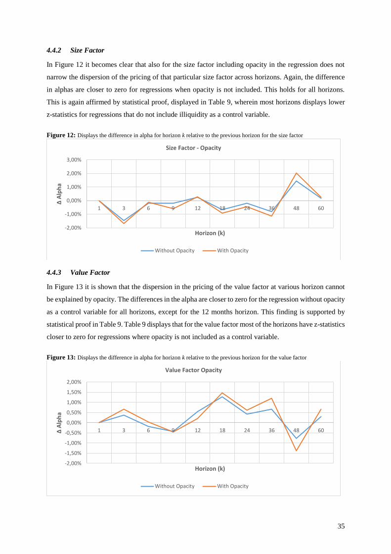
35

4.4.2 Size Factor

In Figure 12 it becomes clear that also for the size factor including opacity in the regression does not

narrow the dispersion of the pricing of that particular size factor across horizons. Again, the difference

in alphas are closer to zero for regressions when opacity is not included. This holds for all horizons.

This is again affirmed by statistical proof, displayed in Table 9, wherein most horizons displays lower

z-statistics for regressions that do not include illiquidity as a control variable.

Figure 12: Displays the difference in alpha for horizon k relative to the previous horizon for the size factor

4.4.3 Value Factor

In Figure 13 it is shown that the dispersion in the pricing of the value factor at various horizon cannot

be explained by opacity. The differences in the alpha are closer to zero for the regression without opacity

as a control variable for all horizons, except for the 12 months horizon. This finding is supported by

statistical proof in Table 9. Table 9 displays that for the value factor most of the horizons have z-statistics

closer to zero for regressions where opacity is not included as a control variable.

Figure 13: Displays the difference in alpha for horizon k relative to the previous horizon for the value factor

-2,00%

-1,00%

0,00%

1,00%

2,00%

3,00%

1 3 6 9 12 18 24 36 48 60

∆ A

lph

a

Horizon (k)

Size Factor - Opacity


-2,00%

-1,50%

-1,00%

-0,50%

0,00%

0,50%

1,00%

1,50%

2,00%

1 3 6 9 12 18 24 36 48 60∆ A

lph

a

Horizon (k)

Value Factor Opacity


36


Figure 14 states that opacity does not help in explaining the dispersion of how the momentum factor is

priced at different horizons. Again the difference in the alphas is closer to zero when opacity is not

included in the regression. This holds for all horizons. The graphical results are again backed with

statistical proof in Table 9. For most horizons of the momentum factor the z-statistics are lower for

regressions without opacity as a control variable.

Figure 14: Displays the difference in alpha for horizon k relative to the previous horizon for the momentum factor


Figure 15 shows that for some horizons opacity can perform as an explanatory variable in explaining

the dispersion of how the profitability factor is priced. The difference in alphas is namely closer to zero

for the 3, 6, and 24 months horizons, when opacity is included in the regression. However, the difference

in alphas for most horizons can be better explained with regressions wherein opacity is not included. So,

the dispersion in the pricing of the profitability factor at various horizons can be better explained by

opacity relative to the other factors. However, the regressions without including opacity generally still

perform better. When looking at statistical evidence in Table 9, it can be observed that there is indeed

more evidence that opacity can explain the dispersion in how the profitability factor is priced. The 3, 6,

9, 12, 24, and 48 months horizons have z-statistics closer to zero for regression that include opacity.

Figure 15: Displays the difference in alpha for horizon k relative to the previous horizon for the profitability factor

-3,00%

-2,00%

-1,00%

0,00%

1,00%

2,00%

1 3 6 9 12 18 24 36 48 60

∆ A

lph

a

Horizon (k)

Momentum Factor - Opacity


-1,00%

-0,50%

0,00%

0,50%

1,00%

1,50%

1 3 6 9 12 18 24 36 48 60

∆ A

lph

a

Horizon (k)

Profitability Factor - Opacity


37


Figure 16 shows that for the investment factor the alphas for some horizons are closer to zero when

incorporating opacity in the regression (e.g. 6, 24, and 48 months horizons). But as concluded for the

profitability factor, the dispersion in the pricing of various horizons for the investment factor can be

generally better explained by the regression wherein opacity is not included. Statistically, there is also

more evidence that opacity can explain the dispersion in how the investment factor is priced. Table 9

shows that at the 3, 6, 9, 24, and 48 months horizons the z-statistics are closer to zero when including

opacity as a control variable. Despite there being more evidence that opacity can explain the dispersion

of how the investment factor is priced, this evidence is not overwhelming.

Figure 16: Displays the difference in alpha for horizon k relative to the previous horizon for the investment factor

-1,50%

-1,00%

-0,50%

0,00%

0,50%

1,00%

1,50%

2,00%

1 3 6 9 12 18 24 36 48 60

∆ A

lph

a

Horizon (k)

Investment Factor - Opacity


38

CHAPTER 5: Conclusion

5.1 Conclusion

Recent literature on investment horizons recognizes dispersion in the pricing of systematic risk factors

at various horizons. This study investigates whether there is indeed dispersion in how six systematic risk

(i.e. the market, size, value, momentum, profitability and investment) factors are priced over various

horizons, through examining data from the Chinese stock market. In other the words, this study tries to

test whether a systematic risk factor is priced at one horizon, where it is not priced at another horizon.

Firstly, this study documents excess returns for the six systematic risk factors at various

horizons. The excess returns fluctuate across horizons for all systematic risk factors, which shows that

there is dispersion in how the systematic risk factors are priced at various horizons. The excess returns

for the market and value factor are significant and negative for generally all horizons. However, the

excess returns are lowest at the intermediate-term horizons, proved by the 12 months horizon that

generates the lowest excess return out of all horizons for both the market and value factor. The

profitability factor has only significant excess returns over the 18, 24, and 36 months horizons, and is

therefore just priced at the relative intermediate-term horizons. The size and the momentum factor

display significant alphas across all horizons, those systematic risk factors are therefore priced at every

horizon examined. The investment factor has significant excess returns only for horizons longer than 12

months. The investment factor seems to be priced over relatively longer horizons.

In addition, this study also reports alphas for the systematic risk factors at various horizons. The

alpha denotes risk-adjusted excess returns relative to a particular asset pricing model or other

benchmark. In this study the benchmark is the Fama-French five-factor model + momentum. This study

reports alpha, because nowadays investors do not just try to reap the highest possible excess return, but

also look to outperform a predetermined benchmark. Also the alphas tend to fluctuate across horizons

for all systematic risk factors, which again shows that there is dispersion in how systematic risk factors

are priced at various horizons. The most significant alphas for the market and value factor can be find

at the longer-term horizons. For the market factor the 36, 48, and 60 months horizons are significant and

positive, and for the value factor horizons longer than 12 months are significant and positive. However,

for both the market and the value factor there are a few significant alphas over relatively shorter horizons

as well (i.e. the 3 months horizon for the market factor, and the 1 and 9 months horizon for the value

factor). The size factor does capture a positive significant alpha at the 1 month horizon and a negative

significant alpha at the 36 months horizon. The momentum factor is positively priced at short-term

horizons, implied by positive and significant alphas at the 1 and 3 months horizons. However, when

moving across longer horizons the 12 and 48 months horizons capture significant negative alphas. The

profitability factor has positive alphas at all horizons examined. And lastly, the investment factor

displays negative alphas at short-term horizons (i.e. 1, 3, 6, and 9 months horizons) and long-term

horizons (i.e. 48 and 60 months horizons).

39

Table 11 provides a summarization of the results for the excess returns and the alphas. Where

the ‘’+’’ and ‘’-‘’ signs display whether the significant excess returns and alphas are positive or negative.

The results concerning the excess returns and alphas have a few implications for investors in

the real world that want to invest in China. Both short-term and long-term horizon investors that aim to

generate significant excess returns should invest in stocks with a high exposure to the size factor and/or

the momentum factor. For both the size and momentum factor all horizons are priced positively and are

therefore profitable. Additionally, long-term horizon investors that aim to obtain positive excess returns,

can safely invest in stocks with a high exposure to the investment factor, because excess returns are

positive and significant for horizons longer than 12 months. Investors should not buy stocks with

exposure to the remaining systematic risk (i.e. market, value, profitability) factors that are, either not

priced, or negatively priced. Investors that try to generate alpha relative to the Fama-French 5–factor

model + momentum, should invest in stock with a high exposure to the market factor if they have

investment horizons of, either 3, 36, 48, or 60 months. Short-term horizon investors that want to reap

alphas should invest in stocks with high exposure to the size factor (positively priced at the 1 month

horizon) or the momentum factor (positively priced at the 1, and 3 months horizons). Long-term horizon

investors that want to obtain alpha should invest in stocks with a high exposure to the value factor, while

alphas are positive and significant for horizons longer than 12 months. An investor also gathers alpha

when buying stocks with high exposure to the profitability factor, irrelevant of the horizon.

Table 7: This table provides an overview of all significant excess returns and alphas found. When a cell is empty it means

that the excess return or alpha appeared not to be significant at a 1% significance level. When a ‘’+’’ is displayed it means

that the excess return or alpha is positive and significant at a 1% significance level, and when a ‘’-‘’ is displayed it means that

the excess return or alpha is negative and significant at a 1% significance level. Again, the alphas are relative to the Fama-

French 5-factor model + momentum.

Overview Results

Market Size Value Momentum Profitability Investment

Horizon Factor Factor Factor Factor Factor Factor

(k) ER α ER α ER α ER α ER α ER α

1 + + - + + + -

3 - + + - + + + -

6 - + - + + -

9 - + - - + + -

12 - + - + - +

18 - + - + + - + +

24 - + - + + - + +

36 - + + - - + + - + +

48 - + + - + + - + + -

60 + + - + + + + -

40

This study did also try explain the dispersion in how horizons were priced over various horizons

by introducing two control variables: illiquidity and opacity. Both graphical and statistical evidence did

not support the view that the two control variables were able to explain the dispersion in how systematic

risk factors are priced over various horizons.

Theoretically, this study shows that there is a possibility of making profits by investing in stocks

that are exposed to certain systematic risk factors at certain horizons. However, in practice, it might be

a bit more complicated to get money out of the Chinese stock market. First of all, China has a stock

market that is underdeveloped and unstable. Therefore, it can be that the profitable nature of certain

systematic risk factors at certain investment horizons are profitable over the used sample period in this

study, but appear to unprofitable in the future. Secondly, the government in China is still heavily

involved in the Chinese stock market. For example, the government restricts investors in China from

short-selling, which limits the opportunities of making high returns in the Chinese stock market. And

lastly, it might be difficult to evaluate systematic risks and make proper portfolio management decisions

in an opaque market like the Chinese stock market, because of the lack of longer track records in Chinese

stocks.

5.2 Limitations

This study tries to explain the dispersion in systematic risk factors with including opacity as a control

variable. As explained before, both the momentum factor and opacity do arise because of an under

reaction to new information. Intuitively, it is expected that when these two variables are in the same

regression they tend to interfere, and have a high level of multicollinearity. However, this study finds

that the two variables are not correlated, and therefore opacity remains in the regression as a control

variable.

Secondly, this study is performed in China, which has relatively young stock markets. For

example, the Shenzhen and the Shanghai stock markets only reopened in 1990. Because of that, the

Chinese stock markets are dominated by relatively small firms. Comparably, Western stock markets

(e.g. NYSE) are more mature and are represented by both relatively small and big firms. Therefore, it

could be that, due to the domination of relatively small firms, the size effect is not that pronounced in

the Chinese stock markets. However, this study reports significant and positive excess returns for all

horizons, therefore the size effect is discernible in this study.

Also, this study looks at systematic risk neglecting business specific risk. Business specific risk

is the type of risk that comes with company or business industry you invest in. For example, the risk

that a firm defaults or the firm skipping a dividend pay-out that was expected. This kinds of risks cannot

be measured by beta. However, these kind of risks can be reduced through diversification.

Finally, this study does also neglect transaction costs and taxes, which will have an impact on

substantially decreasing excess returns. This is especially true for short-term horizon investors that trade

more frequently and therefore have higher transaction costs.

41

5.3 Future research

The quest why systematic risk factors are priced differently across various horizons is still ongoing.

When considering that in this study just two out of many control variables are tested to explain the

dispersion in the pricing of systematic risk factor across horizons, there are much more control variables

that can be tested by academics to explain this dispersion. Alternatively, academics can also try to find

different proxies for illiquidity or opacity that are better able to explain the dispersion in the pricing of

systematic risk factors across horizons.

Furthermore, this study just focuses on how certain individual systematic risk factors are priced.

It might be interesting for future research to combine certain systematic risk factors and see how they

are priced across different horizons.

Another possible extension to this study is incorporating transaction costs and taxes in

calculating the excess returns of a long portfolio over a short portfolio. For example, incorporating

transaction costs can lead to new insights, because a distinction is made in transaction costs for short-

term investors, which are generally higher, and transaction costs for long-term investors, which are

generally lower.

To conclude, the topic of short- and long-term risk in stock markets’ is a relatively new field in

the academic literature. There remains still a lot of room for additional research which could lead to new

interesting insights regarding this topic.

42

REFERENCES

Amihud, Y., Mendelson, H., (1986). Asset Pricing and the Bid-Ask Spread. Journal of Financial

Economics 17 (2), 223 – 249.

Amihud, Y., (2002). Illiquidity and Stock Returns: Cross-Section and Time-Series Effects. Journal of

Financial Markets 5 (1), 31–56.

Black, F., (1972). Capital Market Equilibrium with Restricted Borrowing. Journal of Business 45 (3),

444 – 454.

Boons, M., Tamoni A., (2016). Horizon-Specific Macroeconomic Risks and the Cross Section of

Expected Returns. Working Paper, Available at SSRN:

http://papers.ssrn.com/sol3/papers.cfm?abstract_id=2516251

Breeden, D.T., Gibbons, M.R., Litzenberger, R.H., (1989). Empirical Test of the Consumption-Oriented

CAPM. Journal of Finance 44 (2), 231 – 262.

Brennan, M.J., Zhang, Y., (2013). Capital Asset Pricing with a Stochastic Horizon. Unpublished

working paper, University of California, Los Angeles.

Carhart, M.M., (1997). On Persistence in Mutual Fund Performance. Journal of Finance 52 (1), 57 –

82.

DeAngelo, L. (1986). Accounting Numbers as Market Valuation Substitutes: A Study of Management

Buyouts of Public Stockholders. The Accounting Review 61 (3), 400-420.

Dechow, P.M., Sloan, R., Sweeney, A., (1995). Detecting Earnings Management. The Accounting

Review 70 (2), 193–225.

Demirer, R., Kutan, A.M., (2006). Does Herding Behavior Exist in Chinese Stock Markets? Journal of

International Financial Markets 16 (2), 123–142.

Fama, E.F., French, K.R., (1992). The Cross-Section of Expected Stock Returns. Journal of Financial

and Quantitative Analysis 31 (2), 427 – 465.

Fama, E.F., French, K.R., (2004). The Capital Asset Pricing Model: Theory and Evidence. Journal of

Economic Perspectives 18 (3), 25 – 46.

Fama, E.F., French K.R., (2015). A Five-Factor Asset Pricing Model. Journal of Financial Economics

116 (1), 1 – 22.

43

Gilbert, T., Hrdlicka, C., Kalodimos, J., Siegel, S., (2014). Daily Data is Bad for Beta: Opacity and

Frequency-Dependent Betas. Review of Asset Pricing Studie, 4 (1), 78 – 117.

Healy, P.M. (1985). The Effect of Bonus Schemes on Accounting Decisions. Journal of Accounting and

Economics 7 (1-3), 85-107.

Healy, P., (1996). Discussion of a Market-Based Evaluation of Discretionary Accrual Models. Journal

of Accounting Research 34 (suppl.), 107-115.

Hull, J.C., (2015). Risk management and Financial Institutions. John Wiley & Sons, Inc., New Jersey.

Jegadeesh, N., Titman, S., (1993). Returns to Buying Winners and Selling Losers: Implications for Stock

Market Efficiency. Journal of Finance 48 (1) , 65 – 91.

Jones, J., (1991). Earnings Management During Import Relief Investigations. Journal of Accounting

Research 29 (2), 193-228.

Kamara, A., Korajczyk, R.A., Lou, X., Sadka, R., (2015). Horizon Pricing. Journal of Financial and

Quantitative Analysis, Forthcoming.

Kang, J., Liu M.-H., Ni S.X. (2002). Contrarian and Momentum Strategies in the China Stock Market:

1993-2000. Pacific-Basin Finance Journal 10 (3), 243 – 265.

Lintner, J., (1965). The Valuation of Risk Assets and the Selection of Risky Investments in Stock

Portfolios and Capital Budgets. Review of Economics and Statistics 47 (1), 13 – 37.

Markowitz, H., (1952). Portfolio Selection. Journal of Finance 7 (1), 77 – 91.

Markowitz, H., (1959). Portfolio Selection: Efficient Diversification of Investments. Cowles

Foundation Monograph, New York: John Wiley & Sons, Inc.

Novy-Marx, R., (2013). The Other Side of Value: The Gross Profitability Premium. Journal of Financial

Economics 108 (1), 1 – 28.

Orlik, T., (2015, March 31). China’s Big Stock Market Rally is Being Fueled by High-School Dropouts.

Retrieved from http://www.bloomberg.com

Pettis, M., (2013, November 24). When are Markets ‘’Rational’’? Retrieved from http://

http://www.blog.mpettis.com

44

Reinganum, M.R., (1981). Misspecification of Capital Asset Pricing. Journal of Financial Economics

9 (1), 19 – 46.

Sharpe, W.F., (1964). Capital Asset Prices: A Theory of Market Equilibrium under Conditions of Risk.

Journal of Finance 19 (3), 425 – 442.

Titman, S., Wei, J.K.C., Xie, F., (2004). Capital Investments and Stock Returns. Journal of Financial

Quantitative Analysis 39 (4), 677 – 700.

45

APPENDIX A

Appendix A tends to explain the variables used in this study, by respectively denoting the variable code,

the name of the variable, the definition of the variable, and the source of where the variable is collected

(in italic).

AT – Assets: This item represents the total assets/liabilities of a company at a point in time

Source: WRDS Compustat Global

COGS – Cost of Goods Sold: This item represents all costs directly allocated by the company to

production, such as material, labour and overhead.


CSHOI – Common Shares Outstanding: This issue-level item represents the net number of

common/ordinary shares outstanding as of the company's fiscal year-end.


P – Price: This item represents the official closing monthly price adjusted for dividends, stock splits

and many other changes to make every price comparable over time.

Source: Datastream

PPEGT – Property, Plant and Equipment: This item represents the cost and/or valuation of tangible

fixed assets used in the production of revenue.


RECT – Receivables: This item represents an asset designation applicable to all debts, unsettled

transactions or other monetary obligations owed to a company by its debtors or customers.


REFT – Revenue: This item represents Sales/Turnover (Net) plus Operating Revenues.


SALE – Sales/Turnover: This item represents gross sales (the amount of actual billings to customers

for regular sales completed during the period) reduced by cash discounts, trade discounts, and returned

sales and allowances for which credit is given to customers, for each operating segment.


http://www.investopedia.com/terms/d/debtor.asp

46

TEQ – Stockholders Equity: This item represents the common equity, preferred equity and

nonredeemable non-controlling interest of a company.


TXDITC – Deferred Taxes and Investment Tax Credit: This item represents the accumulated tax

deferrals due to timing differences between the reporting of revenues and expenses for financial

statements and tax forms and investment tax credit.


XINT – Interest and Related Expense: This item represents the periodic expense to the company of

securing short- and long-term debt. Where possible, this item is collected as a gross figure (for example,

if interest expense is reported net by the company, interest income and/or interest capitalized will be

added back to arrive at a gross figure).


XSGA – Selling, General and Administrative Expense: This item represents the sum of all direct and

indirect selling expenses and all general and administrative expenses of a company.


VO – Turnover by Volume: This item represents the monthly turnover by volume, measured in

Chinese Yuan.

Source: Datastream

http://www.investopedia.com/terms/e/expense.asp

http://www.investopedia.com/terms/g/general-and-administrative-expenses.asp

47

ATTACHMENT

Table 8: A z-test is performed to test whether there is a significant difference in the change of alpha spreads for horizon k

relative to horizon k-1. For example, the coefficient of horizon k=3 is the z-statistic based on the difference in alpha spreads

between the 3 months and the 1 month horizon. Both the z-statistics for differences in the alpha spread for regressions without

illiquidity (1) and with illiquidity (2) are given. A lower z-statistic shows that there is less dispersion in one horizon relative

to the previous horizon. The formula of the z-test is given as: 𝑧 = (𝛼2 − 𝛼1) √𝜎12 𝑛1 + 𝜎2

2 𝑛2 ⁄ ⁄⁄ . The sample period is June

1995 – December 2015.

Z-Statistics for Regressions With and Without Illiquidity

Horizon 𝛃𝐤𝐌𝐊𝐓 𝛃𝐤



𝐂𝐌𝐀

(k) (1) (2) (1) (2) (1) (2) (1) (2) (1) (2) (1) (2)

1 2.31 6.14 -3.80 -3.06 0.87 3.85 -4.88 -5.43 0.63 0.60 0.53 -0.08

3 -3.28 -2.08 -0.45 -2.19 -0.37 -1.35 -2.36 -2.57 -0.12 -0.43 -0.51 0.47

6 1.16 0.57 -0.43 -0.76 -0.91 -1.01 0.26 -1.46 1.38 -0.32 -1.29 -0.33

9 -0.21 0.53 0.67 0.10 1.15 3.48 -1.84 -2.67 -0.99 1.14 2.57 -0.74

12 1.34 1.10 -1.70 -0.89 3.08 3.57 1.49 2.72 -0.30 0.46 -0.04 -1.19

18 -0.38 -2.02 -0.44 0.46 1.14 -0.10 -0.53 0.48 0.24 0.97 0.67 1.06

24 3.46 3.15 -1.99 -3.14 1.66 0.86 0.29 3.57 -0.10 0.26 -0.30 -0.21

36 -2.42 -1.96 3.60 5.07 -1.88 -2.14 -0.69 -0.21 2.59 1.61 -2.97 -5.63

48 0.39 -1.30 0.50 0.89 0.80 0.68 1.81 2.68 -0.14 0.88 -0.58 0.65

48

Table 9: A z-test is performed to test whether there is a significant difference in the change of alpha spreads for horizon k

relative to horizon k-1. For example, the coefficient of horizon k=3 is the z-statistic based on the difference in alpha spreads

between the 3 months and the 1 month horizon. Both the z-statistics for differences in the alpha spread for regressions without

opacity (1) and with opacity (2) are given. A lower z-statistic shows that there is less dispersion in one horizon relative to the

previous horizon. The formula of the z-test is given as: 𝑧 = (𝛼2 − 𝛼1) √𝜎12 𝑛1 + 𝜎2

2 𝑛2 ⁄ ⁄⁄ . The sample period is June 1995

– December 2015.

Z-Statistics for Regressions With and Without Opacity




𝐂𝐌𝐀

(k) (1) (2) (1) (2) (1) (2) (1) (2) (1) (2) (1) (2)

1 0.00 0.00 0.00 0.00 0.00 0.00 0.00 0.00 0.00 0.00 0.00 0.00

3 2.31 1.80 -3.80 -3.21 0.87 1.17 -4.88 -5.10 0.63 -0.07 0.53 0.43

6 -3.28 -3.45 -0.45 -0.21 -0.37 0.04 -2.36 -3.02 -0.12 -0.01 -0.51 -0.13

9 1.16 0.74 -0.43 -1.11 -0.91 -0.71 0.26 0.95 1.38 1.14 -1.29 -1.13

12 -0.21 -0.17 0.67 0.56 1.15 0.31 -1.84 -1.89 -0.99 -0.92 2.57 3.08

18 1.34 1.28 -1.70 -1.85 3.08 2.64 1.49 1.27 -0.30 -1.29 -0.04 0.23

24 -0.38 -0.91 -0.44 -0.83 1.14 1.28 -0.53 -0.63 0.24 -0.15 0.67 -0.12

36 3.46 3.78 -1.99 -2.12 1.66 2.25 0.29 -0.44 -0.10 0.55 -0.30 -0.50

48 -2.42 -1.79 3.60 3.86 -1.88 -2.48 -0.69 0.39 2.59 2.19 -2.97 -1.77

60 0.39 -1.34 0.50 0.49 0.80 1.27 1.81 1.74 -0.14 0.37 -0.58 -1.41

49

Table 10: This table reports the level of illiquidity for the top decile (i.e. decile with 10% stocks that have the highest exposure

to a particular risk factor) and the bottom decile (i.e. decile with 10% stocks that have the lowest exposure to a particular risk

factor). Illiquidity is measured by the Amihud illiquidity measure.

Overview Illiquidity Levels at Different Horizons




𝐂𝐌𝐀

(k) D1 D10 D1 D10 D1 D10 D1 D10 D1 D10 D1 D10

1 0.4840 0.4427 0.4669 0.4049 0.4316 0.4285 0.5036 0.4142 0.4067 0.5516 0.5283 0.3890

3 0.5155 0.4626 0.4438 0.4767 0.4690 0.4499 0.4984 0.4330 0.4343 0.5202 0.4578 0.4170

6 0.4691 0.5094 0.4268 0.5222 0.4859 0.4487 0.4978 0.4474 0.4383 0.4756 0.4686 0.3986

9 0.4839 0.4840 0.4293 0.5231 0.4600 0.4470 0.5195 0.4443 0.4188 0.4503 0.4246 0.4354

12 0.5279 0.5099 0.4177 0.5223 0.4559 0.4344 0.5065 0.4436 0.4099 0.4616 0.4278 0.4387

18 0.5502 0.4710 0.4180 0.4672 0.4652 0.4344 0.4702 0.4499 0.4271 0.4809 0.4398 0.4506

24 0.5428 0.4454 0.4248 0.4740 0.4662 0.4391 0.4578 0.4529 0.4114 0.4629 0.4317 0.4450

36 0.4850 0.5198 0.4280 0.4575 0.4469 0.4886 0.4888 0.4167 0.4573 0.4268 0.4412 0.4658

48 0.4818 0.5097 0.4463 0.4600 0.4726 0.4573 0.5242 0.4118 0.4631 0.4467 0.4454 0.4830

60 0.5013 0.4711 0.4447 0.4866 0.5061 0.4362 0.5083 0.4297 0.4615 0.4570 0.4306 0.4852

50

Table 11: This table reports the level of opacity for the top decile (i.e. decile with 10% stocks that have the highest exposure

to a particular risk factor) and the bottom decile (i.e. decile with 10% stocks that have the lowest exposure to a particular risk

factor). Opacity is measured by the variance in discretionary accruals.

Overview Opacity Levels at Different Horizons




𝐂𝐌𝐀

(k) D1 D10 D1 D10 D1 D10 D1 D10 D1 D10 D1 D10

1 0.0078 0.0061 0.0063 0.0105 0.0076 0.0075 0.0088 0.0067 0.0090 0.0058 0.0060 0.0084

3 0.0062 0.0088 0.0065 0.0101 0.0072 0.0084 0.0097 0.0068 0.0086 0.0065 0.0062 0.0086

6 0.0062 0.0081 0.0076 0.0077 0.0072 0.0083 0.0089 0.0068 0.0092 0.0070 0.0068 0.0083

9 0.0065 0.0074 0.0077 0.0068 0.0070 0.0080 0.0090 0.0063 0.0086 0.0067 0.0069 0.0083

12 0.0063 0.0075 0.0077 0.0071 0.0073 0.0072 0.0091 0.0062 0.0083 0.0066 0.0067 0.0085

18 0.0069 0.0073 0.0076 0.0068 0.0069 0.0078 0.0085 0.0066 0.0077 0.0077 0.0065 0.0083

24 0.0068 0.0074 0.0082 0.0064 0.0072 0.0079 0.0084 0.0066 0.0076 0.0069 0.0064 0.0090

36 0.0062 0.0077 0.0087 0.0057 0.0060 0.0085 0.0080 0.0064 0.0083 0.0061 0.0068 0.0076

48 0.0059 0.0077 0.0080 0.0053 0.0060 0.0083 0.0081 0.0063 0.0077 0.0064 0.0074 0.0074

60 0.0063 0.0080 0.0076 0.0064 0.0070 0.0079 0.0074 0.0072 0.0073 0.0074 0.0074 0.0079

Pricing of Risk Factors at Various Horizons · Pricing of Risk Factors at Various Horizons ......

Documents

Transcript of Pricing of Risk Factors at Various Horizons · Pricing of Risk Factors at Various Horizons ......