Rigid Body Simulation - Carnegie Mellon School of …baraff/sigcourse/slidesd.pdf · ·...
57
SD1 SIGGRAPH ’97 COURSE NOTES PHYSICALLY BASED MODELING Rigid Body Simulation David Baraff Robotics Institute and School of Computer Science Rigid Body Simulation Rigid Body Simulation David Baraff David Baraff Robotics Institute and Robotics Institute and School of Computer Science School of Computer Science Carnegie Mellon Carnegie Mellon
Transcript of Rigid Body Simulation - Carnegie Mellon School of …baraff/sigcourse/slidesd.pdf · ·...
SD1SIGGRAPH ’97 COURSE NOTES PHYSICALLY BASED MODELING
Rigid Body Simulation
David BaraffRobotics Institute andSchool of Computer Science
Rigid Body SimulationRigid Body Simulation
David BaraffDavid BaraffRobotics Institute andRobotics Institute andSchool of Computer ScienceSchool of Computer Science
CarnegieMellonCarnegieMellon

SD2SIGGRAPH ’97 COURSE NOTES PHYSICALLY BASED MODELING
Particle MotionParticle MotionParticle Motion
x(t)x(t)
v(t)v(t)

SD3SIGGRAPH ’97 COURSE NOTES PHYSICALLY BASED MODELING
Particle StateParticle StateParticle State
x(t)x(t) v(t)v(t)
Y =Y =
6 7 4 4 8 4 4 6 7 4 4 8 4 4 6 7 4 4 8 4 4 6 7 4 4 8 4 4
Y =x(t)
v(t)
Y =x(t)
v(t)

SD4SIGGRAPH ’97 COURSE NOTES PHYSICALLY BASED MODELING
Particle DynamicsParticle DynamicsParticle Dynamics
F(t)F(t)
v(t)v(t)
x(t)x(t)

SD5SIGGRAPH ’97 COURSE NOTES PHYSICALLY BASED MODELING
State DerivativeState DerivativeState Derivative
v(t)v(t)6 7 4 4 8 4 4 6 7 4 4 8 4 4 6 7 4 4 8 4 4 6 7 4 4 8 4 4
ddt
Y =ddt
x(t)
v(t)
=v(t)
F(t) / m
ddt
Y =ddt
x(t)
v(t)
=v(t)
F(t) / m
F(t) / mF(t) / m
d
dtY =
d
dtY =

SD6SIGGRAPH ’97 COURSE NOTES PHYSICALLY BASED MODELING
Multiple ParticlesMultiple ParticlesMultiple Particles

SD7SIGGRAPH ’97 COURSE NOTES PHYSICALLY BASED MODELING
State DerivativeState DerivativeState Derivative
6n elements6n elements...... ......d
dtY =
d
dtY =
ddt
Y =ddt
x1(t)
v1(t)
M
xn (t)
vn (t)
=
v1(t)
F1(t) / m1
M
vn (t)
Fn (t) / mn
ddt
Y =ddt
x1(t)
v1(t)
M
xn (t)
vn (t)
=
v1(t)
F1(t) / m1
M
vn (t)
Fn (t) / mn

SD8SIGGRAPH ’97 COURSE NOTES PHYSICALLY BASED MODELING
ODE solutionODE solutionODE solution
Y(t0) Y(t0)
Y(t0 + ∆t) Y(t0 + ∆t)
...... Y(t1) Y(t1)
d
dtY(t0 )
d
dtY(t0 )
d
dtY(t0 + ∆t)
d
dtY(t0 + ∆t)

SD9SIGGRAPH ’97 COURSE NOTES PHYSICALLY BASED MODELING
ODE solverODE solver
Y(t0) Y(t0)
t0 t0
t1 t1
dydtdydt
lenlen
void dydt(double t, double y[], double ydot[])
void dydt(double t, double y[], double ydot[])
Y(t1) Y(t1)

SD10SIGGRAPH ’97 COURSE NOTES PHYSICALLY BASED MODELING
dydtdydtdydt
Y(t) = Y(t) =
x1(t)
v1(t)
xn(t)
vn(t)
x1(t)
v1(t)
xn(t)
vn(t)
v1(t)
F1(t)/ m1
vn(t)
Fn(t)/mn
v1(t)
F1(t)/ m1
vn(t)
Fn(t)/mn
d
dtY(t) =
d
dtY(t) =

SD11SIGGRAPH ’97 COURSE NOTES PHYSICALLY BASED MODELING
Rigid Body StateRigid Body StateRigid Body State
v(t)v(t)
x(t)x(t)
Y =
x(t)
?
v(t)
?
Y =
x(t)
?
v(t)
?

SD12SIGGRAPH ’97 COURSE NOTES PHYSICALLY BASED MODELING
Rigid Body Equation of MotionRigid Body Equation of MotionRigid Body Equation of Motion
ddt
Y =ddt
x(t)
?
Mv(t)
?
=
v(t)
?
F(t)
?
ddt
Y =ddt
x(t)
?
Mv(t)
?
=
v(t)
?
F(t)
?
SD13SIGGRAPH ’97 COURSE NOTES PHYSICALLY BASED MODELING
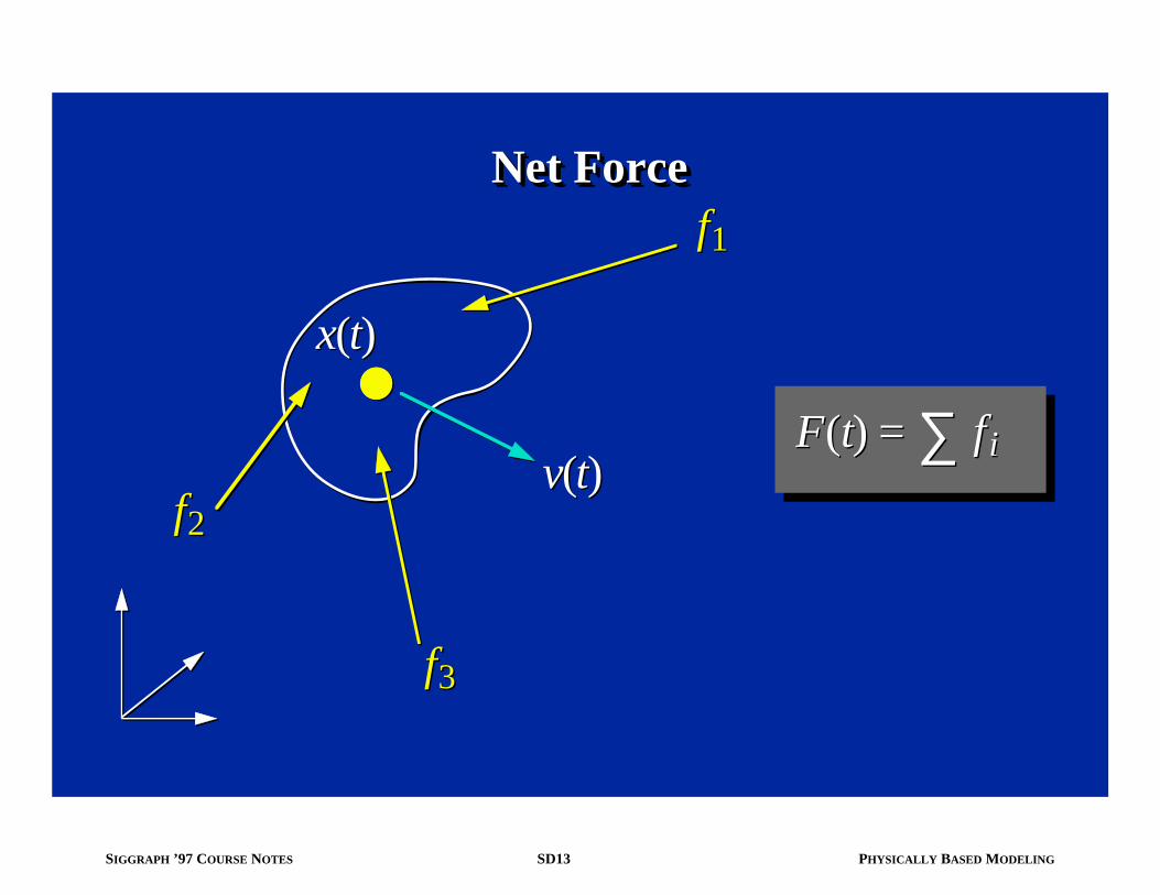
Net ForceNet ForceNet Force
v(t)v(t)
x(t)x(t)
f1 f1
f2 f2
f3 f3
F(t) = fi ∑ F(t) = fi ∑

SD14SIGGRAPH ’97 COURSE NOTES PHYSICALLY BASED MODELING
OrientationOrientationOrientation
We represent orientation as a rotation matrix R(t). Points are transformed from body-space to world-space as:
We represent orientation as a rotation matrix R(t). Points are transformed from body-space to world-space as:
††
††He’s lying. Actually, we use quaternions.He’s lying. Actually, we use quaternions.
p(t) = R(t)p0 + x(t)p(t) = R(t)p0 + x(t)

SD15SIGGRAPH ’97 COURSE NOTES PHYSICALLY BASED MODELING
00
p(t)p(t)
body spacebody space world spaceworld space
x(t)x(t)
p0p0

SD16SIGGRAPH ’97 COURSE NOTES PHYSICALLY BASED MODELING
Angular VelocityAngular VelocityAngular Velocity
We represent angular velocity as a vector ω(t), which encodes both the axis of the spin and the speed of the spin.
We represent angular velocity as a vector ω(t), which encodes both the axis of the spin and the speed of the spin.

SD17SIGGRAPH ’97 COURSE NOTES PHYSICALLY BASED MODELING
Angular Velocity DefinitionAngular Velocity DefinitionAngular Velocity Definition
ω(t)ω(t)
x(t)x(t)
How are R(t) andω(t) related?How are R(t) andω(t) related?

SD18SIGGRAPH ’97 COURSE NOTES PHYSICALLY BASED MODELING
Angular VelocityAngular VelocityAngular Velocity
R(t) and ω(t) are related by R(t) and ω(t) are related by ••
ddt
R(t) =0 −ωz (t) ω y (t)
ωz (t) 0 −ω x (t)
−ωy (t) ω x (t) 0
R(t)ddt
R(t) =0 −ωz (t) ω y (t)
ωz (t) 0 −ω x (t)
−ωy (t) ω x (t) 0
R(t)
(ω(t)* is a shorthand for the above matrix) (ω(t)* is a shorthand for the above matrix)
SD19SIGGRAPH ’97 COURSE NOTES PHYSICALLY BASED MODELING
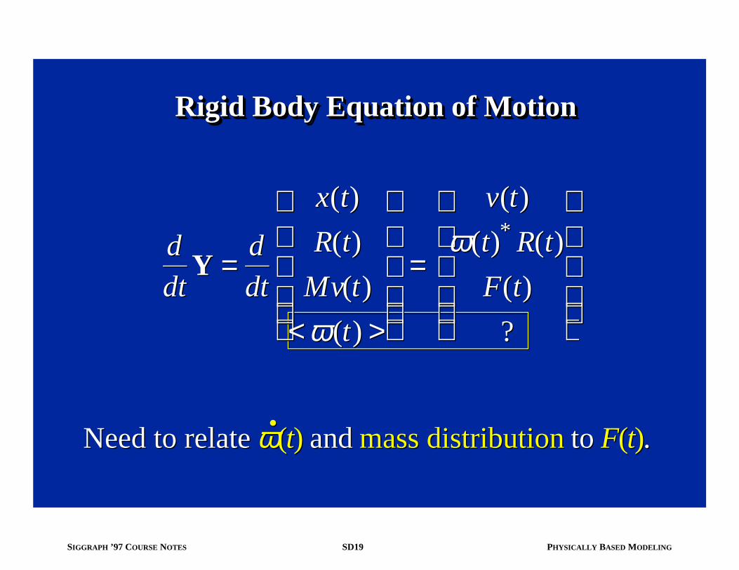
Rigid Body Equation of MotionRigid Body Equation of MotionRigid Body Equation of Motion
Need to relate ω(t) and mass distribution to F(t).Need to relate ω(t) and mass distribution to F(t).••
ddt
Y =ddt
x(t)
R(t)
Mv(t)
< ω(t) >
=
v(t)
ω(t)* R(t)
F(t)
?
ddt
Y =ddt
x(t)
R(t)
Mv(t)
< ω(t) >
=
v(t)
ω(t)* R(t)
F(t)
?

SD20SIGGRAPH ’97 COURSE NOTES PHYSICALLY BASED MODELING
Inertia TensorInertia TensorInertia Tensor
†Integrals are precomputed.†Integrals are precomputed.
I(t) =Ixx Ixy Ix z
Iyx Iyy Iy z
Iz x Iz y Iz z
I(t) =Ixx Ixy Ix z
Iyx Iyy Iy z
Iz x Iz y Iz z
Ixx = M (y2 + z2 )dVV∫Ixx = M (y2 + z2 )dVV∫
off-diagonal terms†off-diagonal terms†diagonal terms†diagonal terms†
Ixy = −M xydVV∫Ixy = −M xydVV∫

SD21SIGGRAPH ’97 COURSE NOTES PHYSICALLY BASED MODELING
Net TorqueNet TorqueNet Torque
x(t)x(t)
f1 f1
f2 f2
f3 f3
p1 p1
p2 p2
p3 p3
τ (t) = (pi − x(t)) × fi∑
τ (t) = (pi − x(t)) × fi∑

SD22SIGGRAPH ’97 COURSE NOTES PHYSICALLY BASED MODELING
ddt
Y =ddt
x(t)
R(t)
Mv(t)
I(t)ω(t)
=
v(t)
ω(t)* R(t)
F(t)
τ (t)
ddt
Y =ddt
x(t)
R(t)
Mv(t)
I(t)ω(t)
=
v(t)
ω(t)* R(t)
F(t)
τ (t)
Rigid Body Equation of MotionRigid Body Equation of MotionRigid Body Equation of Motion
P(t) – linear momentum
L(t) – angular momentum
P(t) – linear momentum
L(t) – angular momentum

SD23SIGGRAPH ’97 COURSE NOTES PHYSICALLY BASED MODELING
What’s in the Course NotesWhat’s in the Course NotesWhat’s in the Course Notes
1. Implementation of 1. Implementation of dydt dydt for rigid bodiesfor rigid bodies
(bookkeeping, data structures, computations) (bookkeeping, data structures, computations)
2. Quaternions – derivations and code2. Quaternions – derivations and code
3. Miscellaneous formulas and examples3. Miscellaneous formulas and examples
4. Derivations for force and torque equations,4. Derivations for force and torque equations,
center of mass, inertia tensor, rotation center of mass, inertia tensor, rotation
equations, velocity/acceleration of points equations, velocity/acceleration of points

SD24SIGGRAPH ’97 COURSE NOTES PHYSICALLY BASED MODELING
ConstraintsConstraintsConstraints
We want rigid bodies to behave as solid objects, We want rigid bodies to behave as solid objects, and not inter-penetrate. By applying and not inter-penetrate. By applying constraintconstraint forces between contacting bodies, we prevent forces between contacting bodies, we prevent interpenetration from occurring. We need to:interpenetration from occurring. We need to:
a) Detect interpenetration a) Detect interpenetration
b) Determine contact points b) Determine contact points
c) Compute constraint forces c) Compute constraint forces

SD25SIGGRAPH ’97 COURSE NOTES PHYSICALLY BASED MODELING
Simulations with CollisionsSimulations with CollisionsSimulations with Collisions
Y(t0) Y(t0)

SD26SIGGRAPH ’97 COURSE NOTES PHYSICALLY BASED MODELING
Simulations with CollisionsSimulations with CollisionsSimulations with Collisions
Y(t0) Y(t0)
Y(t0 + ∆t) Y(t0 + ∆t)

SD27SIGGRAPH ’97 COURSE NOTES PHYSICALLY BASED MODELING
Simulations with CollisionsSimulations with CollisionsSimulations with Collisions
Y(t0) Y(t0)
Y(t0 + ∆t) Y(t0 + ∆t)
Y(t0 +2∆t) Y(t0 +2∆t)

SD28SIGGRAPH ’97 COURSE NOTES PHYSICALLY BASED MODELING
An Illegal State YAn Illegal State YAn Illegal State Y
Y(t0) Y(t0)
Y(t0 + ∆t) Y(t0 + ∆t)
Y(t0 +2∆t) Y(t0 +2∆t)
Y(t0 +3∆t) Y(t0 +3∆t)
illegalstate
illegalstate

SD29SIGGRAPH ’97 COURSE NOTES PHYSICALLY BASED MODELING
Backing up to the Collision TimeBacking up to the Collision TimeBacking up to the Collision Time
Y(tc) Y(tc)

SD30SIGGRAPH ’97 COURSE NOTES PHYSICALLY BASED MODELING
Colliding ContactColliding ContactColliding Contact
pa pa
AA
BB
n • pa < 0 n • pa < 0
pa pa n n

SD31SIGGRAPH ’97 COURSE NOTES PHYSICALLY BASED MODELING
Resting ContactResting ContactResting Contact
pa pa
AA
BB
n n
pa pa
n • pa = 0 n • pa = 0

SD32SIGGRAPH ’97 COURSE NOTES PHYSICALLY BASED MODELING
Collision ProcessCollision ProcessCollision Process
noforceno
forceno
forceno
force
∆t ∆t

SD33SIGGRAPH ’97 COURSE NOTES PHYSICALLY BASED MODELING
A Soft CollisionA Soft CollisionA Soft Collision
forceforce velocityvelocity
∆t ∆t

SD34SIGGRAPH ’97 COURSE NOTES PHYSICALLY BASED MODELING
A Harder CollisionA Harder CollisionA Harder Collision
forceforce velocityvelocity
∆t ∆t

SD35SIGGRAPH ’97 COURSE NOTES PHYSICALLY BASED MODELING
A Very Hard CollisionA Very Hard CollisionA Very Hard Collision
forceforce velocityvelocity
∆t ∆t
SD36SIGGRAPH ’97 COURSE NOTES PHYSICALLY BASED MODELING
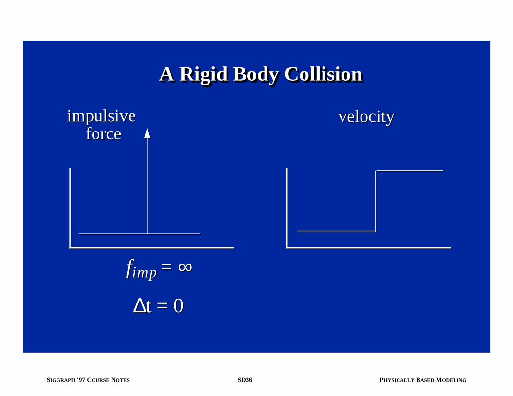
A Rigid Body CollisionA Rigid Body CollisionA Rigid Body Collision
impulsive force
impulsive force
velocityvelocity
fimp = ∞
∆t = 0
fimp = ∞
∆t = 0

SD37SIGGRAPH ’97 COURSE NOTES PHYSICALLY BASED MODELING
Colliding ContactColliding ContactColliding Contact
pa pa
AA
BB
pa pa n n
impulse(alters velocity)
impulse(alters velocity)
SD38SIGGRAPH ’97 COURSE NOTES PHYSICALLY BASED MODELING
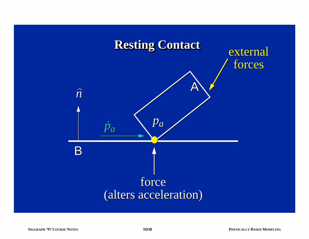
Resting ContactResting ContactResting Contact
pa pa
AA
BB
n n
pa pa
force(alters acceleration)
force(alters acceleration)
externalforces
externalforces

SD39SIGGRAPH ’97 COURSE NOTES PHYSICALLY BASED MODELING
dydt for Solid Objectsdydtdydt for Solid Objects for Solid Objects
Updatecurrentstate
Updatecurrentstate
CollisiondetectionCollisiondetection
Contact pointdeterminationContact pointdetermination
Collision response Collision response
Constraint/friction forcedetermination
Constraint/friction forcedetermination
Penetrationdetected
Estimate:
Penetrationdetected
Estimate: DiscontinuityDiscontinuity
ExceptionsExceptions
Y(t), tY(t), t
tc tc
d
dtY(t)
d
dtY(t)

SD40SIGGRAPH ’97 COURSE NOTES PHYSICALLY BASED MODELING
In the Course Notes – Collision DetectionIn the Course Notes – Collision DetectionIn the Course Notes – Collision Detection
Bounding box check between Bounding box check between nn objects: yes, you objects: yes, you cancan avoid avoid OO((nn22)) work. Don’t even settle for work. Don’t even settle for OO((nn log log n n) ) – insist on an – insist on an OO((nn) ) algorithm!algorithm!
A coherence based collision detection strategy A coherence based collision detection strategy for convex polyhedra: it’s simple, efficient and for convex polyhedra: it’s simple, efficient and (relatively) easy to program.(relatively) easy to program.

SD41SIGGRAPH ’97 COURSE NOTES PHYSICALLY BASED MODELING
Computing ImpulsesComputing ImpulsesComputing Impulses
AA
BB
n n
jn jn
pa– pa–
pa+ = ? pa+ = ?
SD42SIGGRAPH ’97 COURSE NOTES PHYSICALLY BASED MODELING
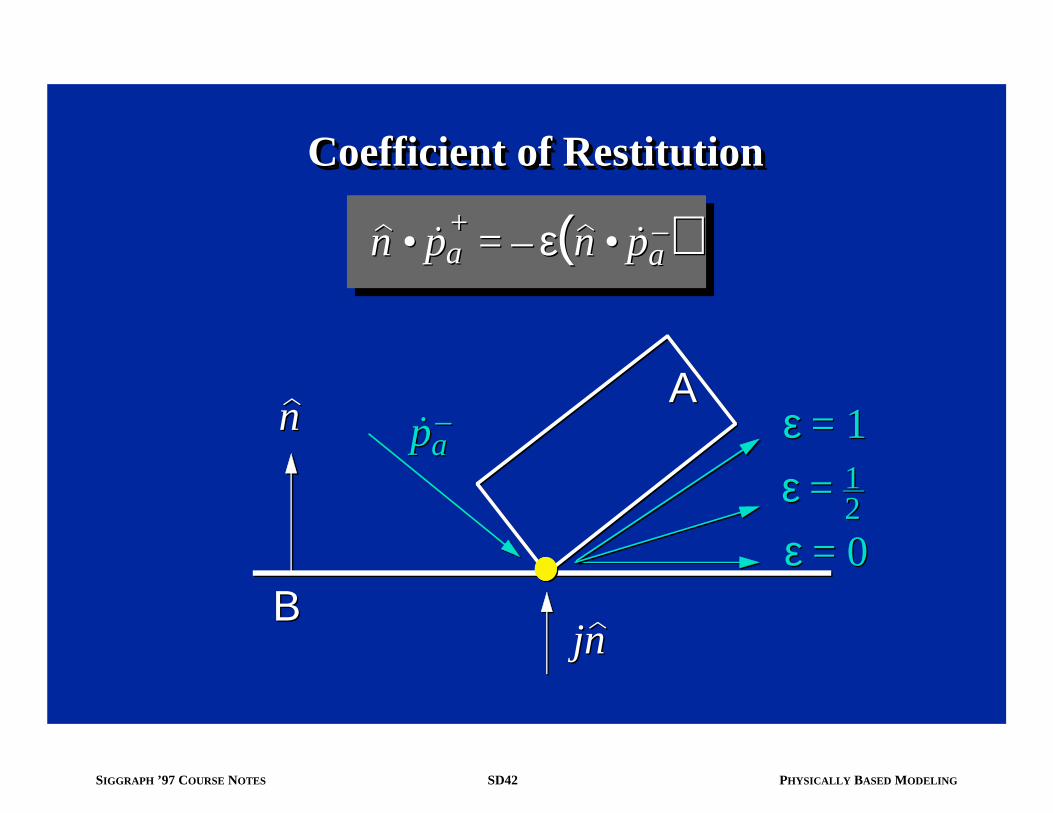
Coefficient of RestitutionCoefficient of RestitutionCoefficient of Restitution
AA
BB
n n
jn jn
pa– pa–
n • pa+
= – ( )ε n • pa– n • pa
+ = – ( )ε n • pa
–
ε = 1 ε = 1
ε = 12 ε = 12
ε = 0 ε = 0

SD43SIGGRAPH ’97 COURSE NOTES PHYSICALLY BASED MODELING
Computing jComputing Computing jj
pa pa
AA
BB
n n
jn jn
cj + b = d cj + b = d n • pa+
= – ( )ε n • pa– n • pa
+ = – ( )ε n • pa
–

SD44SIGGRAPH ’97 COURSE NOTES PHYSICALLY BASED MODELING
Computing jComputing Computing jj
pa pa
AA
n n
BB pb pb jn jn
n • (pa+
– pb+
) = – ( )ε n • (pa– – pb
–) n • (pa+
– pb+
) = – ( )ε n • (pa– – pb
–)

SD45SIGGRAPH ’97 COURSE NOTES PHYSICALLY BASED MODELING
Computing jComputing Computing jj
pa pa
AA
n n
BB pb pb jn jn
n • (pa+
– pb+
) = – ( )ε n • (pa– – pb
–) n • (pa+
– pb+
) = – ( )ε n • (pa– – pb
–) cj + b = d cj + b = d

SD46SIGGRAPH ’97 COURSE NOTES PHYSICALLY BASED MODELING
In the Course Notes – Collision ResponseIn the Course Notes – Collision ResponseIn the Course Notes – Collision Response
Data structures to represent contacts (found by Data structures to represent contacts (found by the collision detection phase).the collision detection phase).
Derivations and code for computing the impulse Derivations and code for computing the impulse between two colliding frictionless bodies for a between two colliding frictionless bodies for a particular coefficient of particular coefficient of ε.ε.
Code to detect collisions and apply impulses.Code to detect collisions and apply impulses.

SD47SIGGRAPH ’97 COURSE NOTES PHYSICALLY BASED MODELING
Resting Contact ForcesResting Contact ForcesResting Contact Forces
pa pa
AA
BB
n n
externalforces
externalforces
f n f n

SD48SIGGRAPH ’97 COURSE NOTES PHYSICALLY BASED MODELING
Conditions on the Constraint ForceConditions on the Constraint ForceConditions on the Constraint Force
To avoid inter-penetration, the force strength f must prevent the vertex pa from accelerating downwards. If B is fixed, this is written as
To avoid inter-penetration, the force strength f must prevent the vertex pa from accelerating downwards. If B is fixed, this is written as
n • pa ≥ 0 n • pa ≥ 0

SD49SIGGRAPH ’97 COURSE NOTES PHYSICALLY BASED MODELING
Computing fComputing Computing ff
pa pa
AA
BB
n n
n • pa ≥ 0 n • pa ≥ 0
f n f n
a f + b ≥ 0 a f + b ≥ 0

SD50SIGGRAPH ’97 COURSE NOTES PHYSICALLY BASED MODELING
Conditions on the Constraint ForceConditions on the Constraint ForceConditions on the Constraint Force
To prevent the constraint force from holding bodies together, the force must be repulsive:
Does the above, along with
sufficiently constrain f ?
To prevent the constraint force from holding bodies together, the force must be repulsive:
Does the above, along with
sufficiently constrain f ?
f ≥ 0 f ≥ 0
n • pa ≥ 0 n • pa ≥ 0 a f + b ≥ 0 a f + b ≥ 0

SD51SIGGRAPH ’97 COURSE NOTES PHYSICALLY BASED MODELING
Workless Constraint ForceWorkless Constraint ForceWorkless Constraint Force
pa pa
AA
BB
n n
Either
or
Either
or
f n f n
a f + b = 0 a f + b = 0
a f + b > 0 a f + b > 0
f ≥ 0
f ≥ 0
f = 0f = 0

SD52SIGGRAPH ’97 COURSE NOTES PHYSICALLY BASED MODELING
Conditions on the Constraint ForceConditions on the Constraint ForceConditions on the Constraint Force
To make f be workless, we use the condition
The full set of conditions is
To make f be workless, we use the condition
The full set of conditions is
f ⋅ (af + b) = 0 f ⋅ (af + b) = 0
f ⋅ (af + b) = 0 f ⋅ (af + b) = 0
f ≥ 0
f ≥ 0
a f + b ≥ 0 a f + b ≥ 0

SD53SIGGRAPH ’97 COURSE NOTES PHYSICALLY BASED MODELING
Multiple Contact PointsMultiple Contact PointsMultiple Contact Points
AA
BB
CC
f1 n1 f1 n1
f2 n2 f2 n2

SD54SIGGRAPH ’97 COURSE NOTES PHYSICALLY BASED MODELING
Conditions on f1Conditions on Conditions on f f11
Workless:Workless:
Non-penetration:Non-penetration: Repulsive:Repulsive:
a11 f1 + a12 f2 + b1 ≥ 0a11 f1 + a12 f2 + b1 ≥ 0 f1 ≥ 0 f1 ≥ 0
f1 ⋅ (a11 f1 + a12 f2 + b1) = 0 f1 ⋅ (a11 f1 + a12 f2 + b1) = 0

SD55SIGGRAPH ’97 COURSE NOTES PHYSICALLY BASED MODELING
Workless:Workless:
Repulsive:Repulsive:
a11 f1 + a12 f2 + b1 ≥ 0
a21 f1 + a22 f2 + b2 ≥ 0
a11 f1 + a12 f2 + b1 ≥ 0
a21 f1 + a22 f2 + b2 ≥ 0 f1 ≥ 0
f2 ≥ 0
f1 ≥ 0
f2 ≥ 0
f1 ⋅ (a11 f1 + a12 f2 + b1) = 0
f2 ⋅ (a21 f1 + a22 f2 + b2) = 0
f1 ⋅ (a11 f1 + a12 f2 + b1) = 0
f2 ⋅ (a21 f1 + a22 f2 + b2) = 0
Non-penetration:Non-penetration:
Quadratic Program for f1 and f2Quadratic Program for Quadratic Program for f f11 and and ff22
SD56SIGGRAPH ’97 COURSE NOTES PHYSICALLY BASED MODELING
In the Course Notes – Constraint ForcesIn the Course Notes – Constraint ForcesIn the Course Notes – Constraint Forces
Derivations of the non-penetration constraints for contacting polyhedra.
Derivations and code for computing the aij and bi coefficients.
Code for computing and applying the constraint forces .
Derivations of the non-penetration constraints for contacting polyhedra.
Derivations and code for computing the aij and bi coefficients.
Code for computing and applying the constraint forces . fi ni fi ni

SD57SIGGRAPH ’97 COURSE NOTES PHYSICALLY BASED MODELING
Quadratic Programs with Equality ConstraintsQuadratic Programs with Equality ConstraintsQuadratic Programs with Equality Constraints
f1 ≥ 0
f2 ≥ 0
f1 ≥ 0
f2 ≥ 0
f1 ⋅ (a11 f1 + a12 f2 + b1) = 0
f2 ⋅ (a21 f1 + a22 f2 + b2) = 0
f1 ⋅ (a11 f1 + a12 f2 + b1) = 0
f2 ⋅ (a21 f1 + a22 f2 + b2) = 0
Non-penetration:Non-penetration: Repulsive:Repulsive:a11 f1 + a12 f2 + b1 0
a21 f1 + a22 f2 + b2 ≥ 0
a11 f1 + a12 f2 + b1 0
a21 f1 + a22 f2 + b2 ≥ 0
==
(free)(free)
Workless:Workless: