Research Collection

Doctoral Thesis

A symplectic homology theory for automorphisms of Liouvilledomains

Author(s): Uljarevic, Igor

Publication Date: 2016

Permanent Link: https://doi.org/10.3929/ethz-a-010654097

Rights / License: In Copyright - Non-Commercial Use Permitted

This page was generated automatically upon download from the ETH Zurich Research Collection. For moreinformation please consult the Terms of use.

ETH Library

DISS. ETH NO. 23378

A S Y M P L E C T I C H O M O L O G Y T H E O RY F O RA U T O M O R P H I S M S O F L I O U V I L L E D O M A I N S

a thesis submitted to attain the degree of

Doctor of Sciences of ETH Zurich

(Dr. sc. ETH Zurich)

presented by

igor uljarevic

Master of Mathematics, University of Belgrade

born on 20.09.1988

citizen of Serbia

accepted on the recommendation of

Prof. Dr. Paul BiranProf. Dr. Dietmar Salamon

Prof. Dr. Alexandru Oancea

2016

To my adorable niece

A C K N O W L E D G M E N T S

I would like to thank my advisers, Paul Biran and Diet-mar Salamon, for their support and encouraging advice.I am grateful to the co-examiner, Alexandru Oancea, forhis efforts and useful comments that improved this thesis.My work greatly profited from many fruitful discussionswith Alberto Abbondandolo, Jonathan David Evans, WillMerry, Juan Carlos Alvarez Paiva, Leonid Polterovich, FelixSchlenk, Peter Uebele, and Otto van Koert.

I would also like to thank Darko Milinkovic for introduc-ing me to the field of symplectic geometry and his lessonson global analysis. I learned the art of problem solving fromFilip Moric. I also appreciate and acknowledge many inter-esting discussions on philosophy and politics that we had.

I am indebted to Nada Kovacevic for my first steps inmath. I still do it with the same enthusiasm she once engen-dered in me.

I express my deep gratitude to Dušan Radosavljevic,Lazar Supic, and my unforgettable teacher, Divna Spaic, forhelping me with numerous linguistic issues. I thank LucaGalimberti for translating the abstract into Italian.

I am grateful to all my fellow PhD students and allgood people that I met in Zurich for making my stay inSwitzerland very pleasant. Especially, Charel Antony, MadsBisgaard, Manuela Gehrig, Pengyu Le, Jonas Lührmann,Vlad Margarint, Thomas Marquardt, Francesco Palmurella,Alexandru-Dumitru Paunoiu, Mario Schulz, Tatjana Simce-vic, Alexander Vitanov, and Micha Thomas Wasem havebeen agreeable distraction from my work.

iii

This thesis would have been far less visually appealing ifit was not for A Classic Thesis Style by André Miede.

Finally, I would like to thank my parents, Mato andNataša, and to my sisters, Dajana and Nina, for being agreat inspiration.

iv

A B S T R A C T

We develop a Floer homology that is tailored for studingautomorphisms of Liouville domains (symplectic mani-folds with contact-type boundaries). The Floer homology,HF∗(W,φ,a), is a graded vector space in Z2 coefficientswhich is associated to an exact symplectomorphim φ ofa Liouville domain W and a real number a that is not aperiod of some Reeb orbit on the boundary ∂W. We callsuch real numbers “admissible slopes.”

We investigate how HF∗(W,φ,a) behaves when the datachanges continuously. In particular, the Floer homologyis invariant (up to isomorphisms) under compactly sup-ported symplectic isotopies of φ and under varying a

through admissible slopes.

Two types of morphisms are significant to the theory, thecontinuation maps and the transfer morphisms. The formerrelate the Floer homologies for different slopes. They havethe following form

HF∗(W,φ,a)→ HF∗(W,φ,b),

where a 6 b, and they make HF∗(W,φ,a) into a directedsystem of graded vector spaces. A transfer morphism

HF∗(W2,φ,a)→ HF∗(W1,φ,b)

is associated to a Liouville domain W2, its codimension-0Liouville subdomain W1, an exact symplectomorphism

v

φ : W1 → W1, and a pair of positive admissible slopes(a,b) such that a 6 b.

The theory turnes out to be efficient for studying the sym-plectic mapping class group. In particular, it leads to cou-ple of criteria for detecting symplectomorphisms that arenot symplectically isotopic to the identity (relative to theboundary). There are also some applications that go beyondsymplectic geometry. Namely, one can find optimal upperbounds for the minimal length of a geodesic on spheres.

vi

R I A S S U N T O

Sviluppiamo un’omologia di Floer appositamente creata alfine di studiare automorfismi di domini di Liouville (va-rietà simplettiche con bordi di tipo contatto). L’omologiadi Floer HF∗(W,φ,a) è uno spazio vettoriale gradato concoefficienti in Z2, a cui vengono associati un simplettomor-fismo esatto φ di un dominio di Liouville W ed un numeroreale a, il quale non risulta essere periodo di qualche or-bita di Reeb sul bordo ∂W. Chiameremo tali numeri reali“pendenze ammissibili”.

Investighiamo il comportamento di HF∗(W,φ,a) al vari-are con continuità dei dati. Nella fattispecie l’omologia diFloer è invariante (a meno di isomorfismi) rispetto ad iso-topie simplettiche a supporto compatto di φ e rispetto avariazioni di a nelle pendenze ammissibili.

Due tipologie di morfismi sono significative per la teoria,ossia le mappe di continuazione ed i morfismi di trasferi-mento. I primi collegano le omologie di Floer con pendenzedifferenti. Assumono la forma seguente

HF∗(W,φ,a)→ HF∗(W,φ,b) ,

ove a 6 b, e rendono HF∗(W,φ,a) un sistema diretto dispazi vettoriali gradati. Ad un morfismo di trasferimento

HF∗(W2,φ,a)→ HF∗(W1,φ,b)

vengono associati un dominio di Liouville W2, il suo sub-dominio di Liouville W1 di codimensione-0, un simpletto-morfismo esatto φ : W1 → W1 ed una coppia di pendenzeammissibili (a,b) tali per cui a 6 b.

vii

La teoria risulta essere efficiente per lo studio del gruppodelle classi di applicazioni simplettiche. In particolare portaad un paio di criteri per individuare simplettomorfismi chenon sono simpletticamente isotopici all’identità (rispetto albordo). Esistono altresì alcune applicazioni che si situanooltre la geometria simplettica, ossia è possibile trovare limitisuperiori ottimali alla lunghezza minimale di una geodeticasu delle sfere.

viii

C O N T E N T S

1 introduction 1

1.1 Transfer morphism 2

1.2 Applications 3

1.3 Conventions 6

2 floer homology for exact symplecto-morphisms 7

2.1 Liouville domains 7

2.2 Floer data and admissible data 8

2.3 Action functional 10

2.4 Grading 12

2.5 Taming infinity 15

2.6 Chain complex 18

2.7 Continuation maps 20

3 invariance under varying data 27

3.1 Dependence on the Liouville form 27

3.2 Varyng the slope 29

3.3 Naturality 30

3.4 Invariance under isotopies 34

4 viterbo’s functoriality 39

4.1 Stair-like Hamiltonians 40

4.2 Construction of the transfer mor-phism 46

5 applications 51

5.1 The symplectic mapping class group 51

5.2 The fibered Dehn twist 53

5.3 Detecting nontrivial mapping classes 60

5.4 Examples 65

5.5 Iterated ratio 69

ix

5.6 Iterated ratio of the fibered Dehn twist onD∗Sn 75

5.7 An application to closed geodesics 81

a technical lemmas 87

x

1I N T R O D U C T I O N

This thesis is devoted to Floer homology for symplectomor-phisms of a Liouville domain. The Floer homology group,HF∗(W,φ,a), is associated to a Liouville domain (W, λ),an exact symplectomorphism φ : W → W (see Defini-tion 2.2.1), and a so-called admissible slope a. An admis-sible slope is any element of R ∪ ∞ that is not a periodof some Reeb orbit on the boundary ∂W. One should thinkof the groups HF∗(W,φ,a) as an extension to the Liouvilledomains of the Floer homology groups in [13]. On the otherhand, these groups also generalize symplectic homology [8,9, 14, 15, 29], in that

SH(W; Z2) = HF(W, id,∞).

The construction of our Floer Homology groups relies ona new variant of the standard action functional, which isadapted to the setting of twisted loops associated to exactsymplectomorphisms (see Section 2.3).

The Floer homology is invariant (up to isomorphisms)under symplectic isotopies of φ that are supported in the in-terior of W. It is also invariant under varying a through ad-missible slopes. However,HF∗(W,φ,a) may change when acrosses a number that is not an admissible slope. This factwill be extensively used in the applications of the theory.Another useful property of the Floer homology is Viterbo’sfunctoriality, which we elaborate on in the following sec-tion.

1

1.1 transfer morphism

In his 1999 paper [29], Viterbo constructed a morphism

SH∗(W2)→ SH∗(W1) (1.1.1)

associated to a codimension-0 embeddingW1 →W2 of a Li-ouville domain into another Liouville domain that respectsthe Liouville forms. The map (1.1.1), called the transfer mor-phism, fits into the commutative diagram

SH∗(W2) SH∗(W1)

H∗+n(W2,∂W2) H∗+n(W1,∂W1).

(1.1.2)

Here, 2n is the dimension of W2 and the map

H∗+n(W2,∂W2)→ H∗+n(W1,∂W1)

is the composition of the homomorphism induced by theinclusion (W2,∂W2) → (W2,W2 \W1) and the excision iso-morphism

H∗+n(W2,W2 \W1)→ H∗+n(W1,∂W1).

The transfer morphism can be extended to the frameworkof the Floer homology for exact symplectomorphism. Thesetting is as follows. Let W1 and W2 be as above, and letφ : W1 → W1 be an exact symplectomorphism. Being com-pactly supported, the symplectomorphism φ can be seen asan exact symplectomorphism of W2 as well (one extends φby the identity).

2

Theorem 1.1.1. LetW1,W2,φ be as above, and let a,b ∈ R+ ∪∞ be positive admissible slopes (with respect to W2 and W1,respectively ). Assume a 6 b. Then, there exists a linear map

HF∗(W2,φ,a)→ HF∗(W1,φ,b),

called the transfer morphism, with the following properties. Itcoincides with the map (1.1.1) for a = b = ∞, and φ equal tothe identity. Moreover, the diagram

HF∗(W2,φ,a) HF∗(W1,φ,b)

HF∗(W2,φ,a ′) HF∗(W1,φ,b ′),

(1.1.3)

consisting of transfer morphisms and continuation maps, com-mutes for all admissible slopes a ′,b ′ ∈ R+ ∪ ∞ such thata 6 a ′, b 6 b ′, and a ′ 6 b ′.

It is noteworthy that the diagrams (1.1.2) and (1.1.3) coin-cide for φ = id, a ′ = b ′ =∞ and a,b > 0 small.

1.2 applications

The theory can be used to detect non-trivial symplecticmapping classes of a Liouville domain (W, λ), i.e. com-pactly supported symplectomorphisms of the Liouville do-main up to symplectic isotopies relative to the boundary.The symplectic mapping classes can be seen as elementsof π0 Sympc(W,dλ), where Sympc(W,dλ) stands for thegroup of all symplectomorphisms of W that are equal tothe identity near the boundary. An important family of suchclasses is furnished by so-called fibered Dehn twists [6, 24]of Liouville domains with periodic Reeb flow on the bound-ary (see Definition 5.2.1).

3

For historical account of symplectic mapping class groupin dimensions 2 and 4, we refer to [25]. The papers [24] and[7] contain further results along these lines also in higherdimensions.

Theorem 5.3.1. Let (W, λ) be a Liouville domain such thatthe Reeb flow on ∂W is 1-periodic. Let a ∈ R be a realnumber that is not a period of any Reeb orbit on ∂W. Ifthe fibered Dehn twist represents a class of order ` ∈ N inπ0 Sympc(W,dλ), then

HF(id,a) ∼= HF(id,a+ `). (5.3.38)

Corolarry 5.3.3. Let (W, λ) be as in Theorem 5.3.1. If

dimH(W; Z2) < dimSH(W; Z2), (5.3.42)

then the fibered Dehn twist represents a class of infiniteorder in π0 Sympc(W,dλ). Here, dimH(W; Z2) stands forthe sum of Betti numbers rather than the dimension of thehomology group of a particular degree.

Special cases of Corollary 5.3.3 include the squares of thegeneralized Dehn twists on T∗Sn and their extensions to thecotangent bundles of other symmetric spaces (see Corollary4.5 in [24]).

Definition 1.2.1. The homology H∗(X; Z2) of a topologicalspace X is said to be symmetric if there exists k ∈ Z suchthat

Hk−j(X; Z2) ∼= Hj(X; Z2)

for all j ∈ Z.

4

Corolarry 5.3.6. Let (W, λ) be as in Theorem 5.3.1. Assumethat the Reeb flow induces a free circle action on ∂W, andthat the first Chern class c1(W) vanishes. If the homologyH∗(W; Z2) is not symmetric, then the fibered Dehn twistrepresents a nontrivial class in π0 Sympc(W,dλ).

The corollary applies when W is a smooth degree d > 2

projective hypersurface in CPm,m > 3 with a neighbour-hood of a smooth hyperplane section removed (see Exam-ple 5.4.8).

We define a numerical invariant, the iterated ratio

κ(W,φ) := lim supm→∞

dimHF(W,φm, ε)m

∈ [0,∞]

of a symplectic mapping class that may be interesting inits own right. It does not depend on the ambient Liouvilledomain in the following sense.

Theorem 5.5.3. Let W1 and W2 be Liouville domains as inTheorem 1.1.1, and let φ :W1 →W1 be an exact symplecto-morphism, then κ(W1,φ) = κ(W2,φ).

Consequently, a generalized Dehn twist furnished by anexact Lagrangian sphere in a Liouville domain always in-duces a class of infinite order (see Corollary 5.6.3).

Theorem 1.1.1 for φ equal to the identity can be used toobtain some information about closed geodesics.

Proposition 1.2.2. Let (Sn,g0) be the n-dimensional spherewith the standard Riemannian metric, and let g be a Riemannianmetric on Sn such that g 6 g0. Then, there exists a non-constantclosed geodesic on (Sn,g) of length less than or equal to 2π.

In fact, a more general statement is true (see Theo-rem 5.7.3 and Corollary 5.7.4).

5

1.3 conventions

Let (W,ω) be a symplectic manifold. A functionH :W → R

and its Hamiltonian vector field XH are related by

dH = ω(XH, ·).

The Hamiltonian isotopy ψHt :W →W of a time-dependentHamiltonian H : R×W → R : (t, x) 7→ Ht(x) is determinedby

∂tψHt = XHt ψ

Ht , ψH0 = id .

An almost complex structure J on W is said to be ω-compatible if ω(·, J·) is a Riemannian metric.

6

2F L O E R H O M O L O G Y F O R E X A C TS Y M P L E C T O M O R P H I S M S

2.1 liouville domains

Definition 2.1.1. A Lioville domain is a compact manifoldW with a 1-form λ, called Liouville form, that satisfies thefollowing conditions. The 2-form dλ is a symplectic form onW, and the Liouville vector field Xλ, defined by Xλydλ = λ,points transversally out on the boundary ∂W.

If (W, λ) is a Liouville domain, then the restriction λ|∂Wof λ to the boundary ∂W is a contact form. Using the flow ofthe Liouville vector field Xλ, a collar neighbourhood of ∂Wcan be identified with ((0, 1]× ∂W, r λ|∂W), where r standsfor the real coordinate.

Definition 2.1.2. Let (W, λ) be a Liouville domain. Thereexists a unique embedding

ι : (0, 1]× ∂W →W

such that ι(1, x) = x and ι∗λ = r λ|∂W . The completionW of (W, λ) is the exact symplectic manifold obtained bygluing W and R+ × ∂W via ι.

If W is a Liouville domain and r ∈ R+, we denote by Wr

the subset of the completion W defined by

Wr := W \((r,∞)× ∂W

).

7

Here, and in the rest of the thesis, the sets R+× ∂W and Ware identified with the corresponding regions in the com-pletion W.

2.2 floer data and admissible data

Definition 2.2.1. A symplectomorphism φ : W → W of aLiouville domain (W, λ) is called exact if it is compactlysupported in the interior of W and if the 1-form φ∗λ− λ isexact.

Given an exact symplectomorphism φ. The definition im-plies that a primitive function of the 1-form φ∗λ− λ is con-stant on the boundary components. We denote by Fφ theone for which the sum of its values on the boundary com-ponents is equal to 0. In the case of a Liouville domainwith connected boundary, this means that Fφ is compactlysupported in the interior of the Liouville domain. The ex-act symplectomorphisms of a Liouville domain (W, λ) forma group, denoted by Sympc(W, λ/d). The functions associ-ated to composition and inverse are given by

Fφ0φ1 = Fφ0 φ1 + Fφ1 ,Fφ−1 = −Fφ φ−1.

(2.2.4)

It is convenient to regard exact symplectomorphisms of aLiouville domain as symplectomorphisms of its completion(one can extend φ by the identity on the complement of theLiouville domain). We will tacitly do so.

Every symplectomorphism generated by a Hamiltonianthat is equal to 0 near the boundary is exact. However, anexact symplectomorphism need not be Hamiltonian or evenisotopic to the identity.

8

Definition 2.2.2. A real number a ∈ R is called admissi-ble with respect to a Liouville domain (W, λ) if it is nota period of any Reeb orbit on the boundary ∂W. Infinity∞ is considered admissible with respect to any Liouvilledomain.

Definition 2.2.3. Let φ be an exact symplectomorphism ofa Liouville domain (W, λ). Floer data for φ is a pair (H, J) ofa (time-dependent) Hamiltonian Ht : W → R and a familyJt of dλ-compatible almost complex structures on W satis-fying the following conditions. H and J are twisted by φ,i.e.

Ht+1 = Ht φ, (2.2.5)

Jt+1 = φ∗Jt. (2.2.6)

In addition, there exists r0 ∈ R+ such that

Ht(x, r) = ar, (2.2.7)

dr Jt(x, r) = −λ, (2.2.8)

on (r0,∞)× ∂W, for some admissible a ∈ R. If we want tospecify the slope, we say “(H, J) is Floer data for (φ,a).”

Remark 2.2.4. Let (W, λ) and J be as in Definition 2.2.3. De-note the contact form λ|∂W by α and the induced contactstructure on ∂W by ξ. Condition (2.2.8) together with dλ-compatibility of Jt implies that Jt|ξ is a compatible complexstructure on the symplectic vector bundle

(ξ,dα)→ ∂W.

Definition 2.2.5. Let φ be an exact symplectomorphism.Floer data (H, J) for φ is said to be regular if H is non-degenerate with respect to φ, i.e.

det(d(φ ψH1 )(x) − id

)6= 0,

9

for all fixed points x of φ ψH1 , and if the linearized op-erator for every solution of the Floer equation (2.3.11) onpage 12 is surjective.

2.3 action functional

Definition 2.3.1. [20]. Let φ be an exact symplectomor-phism of a Liouville domain (W, λ), and let Ht : W → R

be a Hamiltonian satisfying (2.2.5). The action functionalAφ,H is a function defined on the twisted loop space

Ωφ := γ : R→ W | φ(γ(t+ 1)) = γ(t)

by

Aφ,H(γ) := −

∫10

(γ∗λ+Ht(γ(t))dt) − Fφ(γ(1)).

Proposition 2.3.2. Let φ and Ht be as in Definition 2.3.1. Thecritical points of the action functional Aφ,H are Hamiltoniantwisted loops, i.e. the elements of the set

Pφ,H :=γ ∈ Ωφ | γ = XHt γ

.

Proof. Let γ ∈ Ωφ and let ζ ∈ TγΩφ. This means ζ is asection of the vector bundle γ∗TW such that

dφ(ζ(t+ 1)) = ζ(t). (2.3.9)

The derivative of Aφ,H at the point γ in the direction ζ isgiven by

dAφ,H(γ)ζ =d

ds

∣∣∣∣s=0

Aφ,H(γs),

10

where γs is a smooth family of twisted loops satisfying

d

ds

∣∣∣∣s=0

γs(t) = ζ(t).

Since

d

ds

∣∣∣∣s=0

(γ∗sλ) = dλ (ζ(t), γ(t))dt+d

dt(λ(ζ(t)))dt,

d

ds

∣∣∣∣s=0

Ht(γs(t)) = dHt(ζ(t))

= −dλ(ζ(t),XHt(γ(t))),

and

d

ds

∣∣∣∣s=0

Fφ(γs(1)) = dFφ(ζ(1))

= (φ∗λ− λ) (ζ(1))

= λ(dφ(ζ(1))) − λ(ζ(1))

~= λ(ζ(0)) − λ(ζ(1)),

we get

dAφ,H(γ)ζ =

∫10

ω (γ(t) −XHt(γ(t)), ζ(t))dt. (2.3.10)

Here, ~ used (2.3.9). Since (2.3.10) holds for all ζ ∈ TγΩφ,we have dAφ,H(γ) = 0 if, and only if, γ(t) = XHt(γ(t)) forall t.

Let (W, λ) be a Liouville domain. A family Jt of dλ -compatible almost complex structures on W which satis-fies (2.2.6) gives rise to a Riemannian metric on Ωφ. TheRiemannian metric is given by

〈ξ, ζ〉 :=∫10

ω(ξ(t), Jt γ(t)ζ(t))dt,

11

where γ ∈ Ωφ is a twisted loop, and ξ, ζ ∈ TγΩφ. The neg-ative gradient flow lines of Aφ,H with respect to this innerproduct are solutions u : R2 → W of the Floer equation

∂su+ Jt(u) (∂tu−XHt(u)) = 0. (2.3.11)

that satisfy the periodicity condition

φ u(s, t+ 1) = u(s, t). (2.3.12)

2.4 grading

Let φ : W → W be a symplectomorphism of a symplecticmanifold (W,ω). Let

Hit : W → R, i = 0, 1

be two Hamiltonians such that

Hit+1 = Hit φ

and such that

det(d(φ ψHi1 )(x) − id

)6= 0,

for all fixed points x of φ ψHi1 . And, let

γi ∈ P(φ,Hi), i = 0, 1

be twisted loops representing the same class in π0Ωφ. Con-sider a homotopy

[0, 1]×R→ W

between them through Ωφ. Write it as a map

u : R×R→ W

12

such that

u(s, t) = φ u(s, t+ 1), (2.4.13)

and

u(s, t) =

γ0(t) for s 6 0

γ1(t) for s > 1.(2.4.14)

Definition 2.4.1. Let u be as above. The relative Maslovindex of u is the number

µ(u) = µCZ(Ψ1) − µCZ(Ψ

0) ∈ Z,

where

Ψi : [0, 1]→ Sp(2n), i ∈ 0, 1,

is the path

t 7→ T−1i,t dψHi

t (γi(0))Ti,0

of symplectic matrices, and

Ts,t : R2n → Tu(s,t)W

is a symplectic trivialization satisfying

dφ Ts,t+1 = Ts,t.

The number µ(u) does not depend on the choice of trivial-ization.

We need the notion of a mapping torus in order to definethe relative Maslov index for the pair (γ0,γ1) (independentof the choice of homotopy u).

13

Definition 2.4.2. Let φ and (W,ω) be as above. The map-ping torus of φ is the fibration pφ : Wφ → S1 defined by

Wφ :=W ×R

(φ(x), t) ∼ (x, t+ 1), pφ([x, t]) := [t] ∈ R/Z.

Denote the vertical tangent bundle of Wφ by

TVW := kerdpφ → Wφ.

The symplectic form ω on W makes TVW into a symplecticvector bundle. A loop in Ωφ, seen as a map

u : R/Z×R→ W

satisfying φ u(s, t+ 1) = u(s, t), can be identified with themap

R/Z×R/Z→ Wφ : (s, t) 7→ [(u(s, t), t)].

Let θ ∈ π0Ωφ. Associated to it is the minimal Chern num-ber Nθ. It is defined as the minimal positive generator ofthe group

NθZ :=⟨c1(T

VW),π1(Ωφ, θ)⟩⊂ Z.

We define the minimal positive generator of trivial group tobe∞, and Z∞ := Z.

Definition 2.4.3. Let W,φ,Hi be as above. The relativeMaslov index for a pair

(γ0,γ1) ∈ P(φ,H0)×P(φ,H1)

of twisted loops representing the same class θ ∈ π0Ωφ isthe number

µ(γ0,γ1) := µ(u) (mod 2Nθ) ∈ Z2Nθ ,

14

where

u : R×R→ W

is such that (2.4.13) and (2.4.14) hold.

2.5 taming infinity

Definition 2.5.1. Let φ be an exact symplectomorphism ofa Liouville domain (W, λ), and let (H−, J−) and (H+, J+) beregular Floer data for φ. Continuation data from (H−, J−)to (H+, J+) consists of Hamiltonians Hs,t,Gs,t : W → R

and a family of dλ-compatible almost complex structuresJs,t on W such that the following conditions are satisfied.For each s ∈ R, Hs,Gs and Js are twisted by φ, i.e.

Hs,t φ = Hs,t+1,

Gs,t φ = Gs,t+1,

and

φ∗Js,t = Js,t+1.

In addition, there exist r0 ∈ (0,∞) and a function

a : R2 → R

that is increasing with respect to the first coordinate suchthat

Gs,t(x, r) = 0,

Hs,t(x, r) = a(s, t)

and the condition (2.2.8) holds for Js(x, r), for all s, t ∈ R,r > r0, and x ∈ ∂W. Finally,

(Hs,t,Gs,t, Js,t) = (H±t , 0, J±t ), for ± s >> 0.

15

Remark 2.5.2. We can find continuation data from (H−, J−)to (H+, J+) whenever the slope of H− is less than or equalto the slope of H+.

Definition 2.5.3. Let φ,Hs,t,Gs,t and Js,t be as in Defini-tion 2.5.1. The energy of a solution u : R2 → W of thes-dependent (generalized) Floer equation

∂su−XGs,t(u) + Js,t(u)(∂tu−XHs,t(u)

)= 0 (2.5.15)

satisfying periodicity condition (2.3.12) is defined to be

E(u) :=

∫∞−∞∫10

∣∣∂su−XGs,t(u)∣∣2Jdtds.

Lemma 2.5.4. Let (W, λ),φ,H±, J±,Hs,Gs, Js be as in Defini-tion 2.5.1, let γ± ∈ P(φ,H±) and let u : R2 → W be a solutionof (2.5.15), (2.3.12) such that lims→±∞ u(s, t) = γ±(t). Then,

E(u) =Aφ,H−(γ−) −Aφ,H+(γ+)−

−

∫∞−∞∫10

Bs,t(u)dtds(2.5.16)

where

Bs,t := ∂sHs,t − ∂tGs,t − Gs,t,Hs,t,

and Gs,t,Hs,t := dλ(XGs,t ,XHs,t) stands for the Poissonbracket.

Proof. Denote by ω the symplectic form dλ. Using (2.5.15),we get∣∣∂su−XGs,t(u)

∣∣2J=

= ω(∂su−XGs,t(u), Js,t(u)(∂su−XGs,t)

)= ω

(∂su−XGs,t(u),∂tu−XHs,t(u)

)= u∗ω+ dHs,t(∂su) − dGs,t(∂tu)+

+ Gs,t,Hs,t(u).

(2.5.17)

16

By the chain rule,

dHs,t(∂su) = ∂s (Hs,t(u)) − (∂sHs,t)(u), (2.5.18)

and similarly

dGs,t(∂tu) = ∂t(Gs,t(u)) − ∂tGs,t(u).

The Stokes theorem implies∫+∞−∞∫10

u∗ωdtds =

=

∫10

(γ+)∗λ−

∫+∞−∞ λ(∂su(s, 1))ds−

−

∫10

(γ−)∗λ+

∫+∞−∞ λ(∂su(s, 0))ds

=

∫10

(γ+)∗λ−

∫10

(γ−)∗λ+

+

∫+∞−∞ (φ∗λ− λ) (∂su(s, 1))ds

=

∫10

(γ+)∗λ−

∫10

(γ−)∗λ+

+ Fφ γ+(1) − Fφ γ−(1).

(2.5.19)

By Newton-Leibniz formula and (2.5.18), we get∫+∞−∞∫10

dHs,t(∂su)dtds =

=

∫+∞−∞∫10

∂s (Hs,t(u)) − (∂sHs,t)(u)dtds

=

∫10

Hs,t γ+(t)dt−∫10

Hs,t γ−(t)dt−

−

∫+∞−∞∫10

(∂sHs,t)(u)dtds.

(2.5.20)

17

Similarly,∫+∞−∞∫10

dGs,t(∂su)dtds =

=

∫+∞−∞∫10

∂t(Gs,t(u)) − ∂tGs,t(u)dtds

=

∫+∞−∞ Gs,1(u(s, 1)) −Gs,0(u(s, 0))ds−

−

∫+∞−∞∫10

∂tGs,t(u)dtds

= −

∫+∞−∞∫10

∂tGs,t(u)dtds.

(2.5.21)

The lemma follows from (2.5.17), (2.5.19), (2.5.20), and(2.5.21).

Lemma 2.5.5. Let W,Hs,t,Gs,t, Js,t and r0 be as in Defini-tion 2.5.1, and let u : U → (r0,∞) × ∂W be a solution of(2.5.15), where U ⊂ R2 is open and connected. Then r u has nolocal maxima unless it is constant.

Proof. The lemma follows from the standard argument,which can be found, for example, in [30].

2.6 chain complex

Theorem 2.6.1. Let φ be an exact symplectomorphism of a Liou-ville domain (W, λ), let (H, J) be regular Floer data for φ, and letγ−,γ+ ∈ P(φ,H). Then, the set

M(φ,H, J,γ−,γ+)

of maps u : R2 → W such that (2.3.11) and (2.3.12) hold, andsuch that

lims→±∞u(s, t) = γ±(t)

18

is a manifold (possibly empty or with connected components ofvarying dimensions). The connected component containing u0has dimension equal to µ(u0). The quotient of the k−dimensionalpart Mk(· · · ) of M(· · · ) by the natural R−action is denoted byMk(· · · ).

Proof. See page 21.

Theorem 2.6.2. In the situation of Theorem 2.6.1, the setM1(φ,H, J,γ−,γ+) is finite. Its cardinality modulo 2 is denotedby n(φ,H, J,γ−,γ+).

Proof. See page 21.

Theorem 2.6.3. Let φ be an exact symplectomorphism of a Li-ouville domain (W, λ), let (H, J) be regular Floer data for φ, letθ ∈ π0Ωφ, and let

γ0 ∈ Pθ(φ,H) := P(φ,H)∩ θ.

Then,

(CF∗(φ,H, J, θ),∂H,J)

is a Z2Nθ-graded chain complex (see page 14 for the definition ofNθ), where

CFk(φ,H, J, θ) :=⊕

γ ∈ Pθ(φ,H)

µ(γ,γ0) = k

Z2 〈γ〉 ,

and ∂ = ∂H,J is defined by

∂ 〈γ〉 :=∑

γ ′ ∈ Pθ(φ,H)

µ(γ,γ ′) = 1

n(φ,H, J,γ,γ ′)⟨γ ′⟩

.

19

We denote the homology of this complex by

HF∗(φ,H, J, θ).

Note that the grading depends on the choice of γ0.

Proof. See page 21.

2.7 continuation maps

Theorem 2.7.1. Let φ be an exact symplectomorphism of a Liou-ville domain (W, λ), let (Hα, Jα) and (Hβ, Jβ) be regular Floerdata for φ, and let

γα ∈ P(φ,Hα), γβ ∈ P(φ,Hβ).

Then, for generic continuation data (Hs,Gs, Js) from (Hα, Jα)to (Hβ, Jβ), the set

M(φ, Hs,Gs, Js,γα,γβ)

of maps u : R2 → W such that (2.5.15) and (2.3.12) hold, andsuch that

lims→−∞u(s, t) = γα(t),

lims→+∞u(s, t) = γβ(t)

is a manifold (cut out transversely by the Floer equation). Theconnected component containing u0 has dimension µ(u0). Thek-dimensional part of M(· · · ) is denoted by Mk(· · · ).

Proof. See page 21.

Theorem 2.7.2. In the situation of Theorem 2.7.1, the setM0(φ, Hs,Gs, Js,γα,γβ) is finite. Its cardinality modulo 2 isdenoted by n(φ, Hs,Gs, Js,γα,γβ).

20

Proof. See below.

Theorem 2.7.3. Let φ,Hα,Hβ,Hs,Gs, Jα, Jβ, Js be as in Theo-rem 2.7.1. Then the linear map

CF∗ (φ,Hα, Jα, θ)→ CF∗(φ,Hβ, Jβ, θ

)defined on generators by

〈γα〉 7→∑

γβ ∈ Pθ(φ,Hβ)

µ(γβ,γα) = 0

n(φ, Hs,Gs, Js,γα,γβ)⟨γβ⟩

induces a homomorphism, called continuation map, on homol-ogy level. The continuation map

Φβα : HF∗

(φ,Hα, Jα, θ

)→ HF∗

(φ,Hβ, Jβ, θ

)does not depend on the choice of continuation data. Moreover, itsatisfies the composition formula

Φγβ Φβα = Φγα, Φαα = id .

Proof. See below.

Corollary 2.7.4. Let φ be an exact symplectomorphism of a Liou-ville domain (W, λ), and let θ ∈ π0Ωφ. If (Hα, Jα) and (Hβ, Jβ)are regular Floer data for φ, and Hα,Hβ have the same slope,then

HF∗ (φ,Hα, Jα, θ) ∼= HF∗(φ,Hβ, Jβ, θ

).

Proof of Theorems 2.6.1, 2.6.2, 2.6.3, 2.7.1, 2.7.2 and 2.7.3.We prove that there exist compact subsets K(φ,H, J) andK(φ, Hs,Gs, Js) of W such that all elements of the Moduli

21

spaces M(φ,H, J,γ−,γ+) and M(φ, Hs,Gs, Js,γα,γβ)map R2 into K(φ,H, J) and K(φ, Hs,Gs, Js), respec-tively. Since M(φ,H, J,γ−,γ+) is a special case ofM(φ, Hs,Gs, Js,γα,γβ) (for Hs, Js s-independent,Gs = 0, γ− = γα, and γ+ = γβ),we consider only the caseof M(φ, Hs,Gs, Js,γα,γβ). The boundary ∂W is denotedshortly by M.

Let r0 ∈ (1,∞) be such that

Gs,t(x, r) = 0, Hs,t(x, r) = a(s, t),

and condition (2.2.8) holds for Js(x, r), for all s, t ∈ R, and(r, x) ∈ (r0,∞) ×M. The existence of such r0 is guaran-teed by the definition of continuation data (Definition 2.5.1).Since the slopes of Hα and Hβ are admissible, the elementsof the sets Pφ,Hα and Pφ,Hβ are contained in the compactset W \

((r0,∞) ×M

). Assume there exist γα ∈ Pφ,Hα ,

γβ ∈ Pφ,Hβ , and u ∈M(φ, Hs,Gs, Js,γα,γβ) such that

u(R2)∩ (r0 + 1,∞)×M 6= ∅.

The symplectomorphism φ is equal to the identity on(r0,∞)×M. Therefore

u(s, t) = u(s, t+ 1)

whenever u(s, t) ∈ (r0,∞)×M. This together with

lims→−∞u(s, t) = γα(t),

lims→+∞u(s, t) = γβ(t)

implies that the sets

u([−C,C]× [0, 1])∩((r0,∞)×M

)

22

and

u(R2)∩((r0,∞)×M

)coincide for C ∈ (0,∞) large enough. Since

[−C,C]× [0, 1]

is a compact set, the function r u attains a maximumon u−1((r0,∞) ×M). Let U ⊂ u−1((r0,∞) ×M) be theconnected component of a point at which the maximumis achieved. Connected components of a locally path-connected space are open. Hence U is an open subset ofu−1((r0,∞)×M). Since u−1((r0,∞)×M) is open in R2, Uis an open subset of R2 as well.

Lemma 2.5.5 implies that r u|U is constant. Denote byc ∈ (0,∞) the value of r u on U. The set U is a connectedcomponent of u−1(c ×M). It follows that U is a closedsubset of u−1(c×M). Since u−1(c×M) is closed in R2,so is U. This implies that U is a non-empty open and closedsubset of R2, i.e. U = R2. However, this is impossible be-cause

lims→+∞u(s, t) = γβ(t).

Since everything happens in a compact subset of W, thearguments for the case of a closed symplectic manifold (in-stead of W) apply here as well [12, 13].

We end the proof by two remarks. Bubbling-off cannot oc-cur because the symplectic form on W is exact. Lemma 2.5.4implies that elements of M(φ, Hs,Gs, Js,γα,γβ) have uni-formly bounded energy.

23

Definition 2.7.5. Let φ be an exact symplectomorphism of aLiouville domain (W, λ), and let θ ∈ Ωφ. For a fixed admis-sible slope, the groups HF∗(φ,H, J, θ) are canonically iso-morphic to each other via the continuation maps. Hencethe group

HF∗(φ,a, θ)

is well defined. We define

HF∗(φ,a) :=⊕

θ∈π0Ωφ

HF∗(φ,a, θ).

Definition 2.7.6. Let φ and θ be as in Definition 2.7.5. Thecontinuation maps give rise to a homomorphism (which wecall the same)

HF∗(φ,a1, θ)→ HF∗(φ,a2, θ) (2.7.22)

whenever a1 6 a2. The groups HF∗(φ,a, θ), where a ∈ R

goes through all admissible slopes, together with homomor-phisms (2.7.22) form a directed system of groups. We define

HF∗(φ,∞, θ) := lim−→a

HF∗(φ,a, θ),

HF∗(φ,∞) :=⊕

θ∈π0Ωφ

HF∗(φ,∞, θ).

Example 2.7.7. In the case of φ = id, we can identify thegroups HF(φ,a), for certain slopes a, with known groups.By construction, HF(id,∞) is equal to the symplectic ho-mology of W with Z2 coefficients

HF(id,∞) = SH(W; Z2).

Since the Floer homology for C2-small Hamiltonian reducesto Morse homology, we get

HF∗(id, ε) ∼= H∗+n(W,M; Z2),

24

and

HF∗(id,−ε) ∼= H∗+n(W; Z2)

for ε > 0 small enough (cf. [17, Theorem 3.9]). Also

HF∗(id, ε, θ) = 0

for θ ∈ π0Ωφ non-trivial and |ε| small.

25

3I N VA R I A N C E U N D E R VA RY I N G D ATA

3.1 dependence on the liouville form

In the next two lemmas, we prove that the Floer homol-ogy HF∗(W,φ,a) remains the same if we change the Li-ouville form by adding an exact 1-form that is compactlysupported in the interior of W. When dealing with dif-ferent Liouville forms on the same manifold, we will in-clude the Liouville form as part of the data for Floer homol-ogy. I.e. the notation HF∗(W, λ,φ,a) will be used instead ofHF∗(W,φ,a).

Lemma 3.1.1. Let (W, λ) be a Liouville domain, and let f :W →R be a function. Then, a map φ : W → W is an exact symplec-tomorphism of (W, λ) if, and only if, it is an exact symplectomor-phism of (W, λ+ df).

Proof. Denote the 1-form λ+ df by λ. Assume φ is an exactsymplectomorphism of (W, λ). Then, there exists a functionF :W → R such that

φ∗λ− λ = dF,

and φ is compactly supported. Hence

φ∗λ− λ = φ∗(λ+ df) − λ− df

= φ∗λ− λ+ d(f φ− f)

= d(F+ f φ− f),

i.e. φ is an exact symplectomorphism of (W, λ). The oppo-site direction is proven analogously.

27

Proposition 3.1.2. Let φ : W → W be an exact symplectomor-phism of a Liouville domain (W, λ), and let f : W → R be afunction equal to 0 near the boundary. Then,

HF∗(W, λ,φ,a) ∼= HF∗(W, λ+ df,φ,a),

for all admissible slopes a.

Proof. Denote by λ the 1-form λ+ df. Since λ and λ agreenear the boundary (where f is equal to 0), the slope of aHamiltonian with respect to (W, λ) is the same as the onewith respect to (W, λ). Moreover, the completions of (W, λ)and (W, λ) are symplectomorphic. Let H be a Hamiltonianwith the slope equal to a. Denote by Fφ the compactly sup-ported function W → R such that

φ∗λ− λ = dFφ.

The functions Fφ and Fφ are related by

Fφ = Fφ + f φ− f.

The lemma follows from the following sequence of equali-ties

Aφ,H(γ) := −

∫10

(γ∗λ+Ht(γ(t))dt

)− Fφ(γ(1))

=Aφ,H(γ) −

∫10

d

dt(f γ)dt− f φ(γ(1))+

+ f(γ(1))

=Aφ,H(γ) − f(γ(1)) + f(γ(0)) − f φ(γ(1))++ f(γ(1))

=Aφ,H(γ),

for γ ∈ Ωφ.

28

3.2 varyng the slope

Proposition 3.2.1. Let φ be an exact symplectomorphism of aLiouville domain (W, λ), and let a1 and a2 be real numbers suchthat elements of the interval [a1,a2] are all admissible. Then

HF∗(φ,a1, θ) ∼= HF∗(φ,a2, θ)

for all θ ∈ π0Ωφ. Moreover, the isomorphism is realized by thecontinuation map.

Proof. Let (H, J) be regular Floer data for (φ,a1). Assumethat conditions (2.2.7) and (2.2.8) hold on (r0,∞)× ∂W. Letχ : (r0,∞) → [0, 1] be a smooth function equal to 0 nearr0 and 1 near ∞, and such that χ ′ ∈ [0, 1]. Consider theHamiltonian H : R× W → R defined by

Ht(x, r) := a1 + (a2 − a1)χ(r),

for (r, x) ∈ (r0,∞)× ∂W, and H = H on Wr0 . The functionr u satisfies the maximum principle, where u is a solu-tion of the Floer equation corresponding to the pair (H, J)(see Proposition 4.1 in [30]). Moreover, there is no elementof P

φ,H intersecting (r0,∞)× ∂W. This implies that ingre-

dients for the definition of HF∗(φ, H, J, θ) are all containedin the compact set Wr0 , where H and H coincide. Hence,the chain complexes CF∗(φ,H, J, θ) and CF∗(φ, H, J, θ) areidentical. Moreover, for generic (H, J), the map

CF∗(φ,H, J, θ) 3 v 7→ v ∈ CF∗(φ, H, J, θ)

can be seen as the continuation map induced by the contin-uation data that is constant with respect to s-coordinate inWr0 . This finishes the proof.

29

3.3 naturality

The naturality is a way to construct isomorphisms betweenFloer homologies for certain pairs of Floer data. The iso-morphisms are furnished by the change of variables usingHamiltonian isotopies, and they do not agree with the con-tinuation maps in general. The naturality plays a crucialrole in the next section, where we prove that the Floer ho-mology is invariant under isotopies of exact symplectomor-phisms. It is also an important ingredient in all of our ap-plications.

Let ψtt∈R be an isotopy of a manifold W, let

H : R× W → R : (t, x) 7→ Ht(x)

be a smooth function, and let Jtt∈R be a family of almostcomplex structures on W. We define ψ∗H to be the smoothfunction

ψ∗H : R× W → R : (t, x) 7→ H(t,ψt(x)),

and ψ∗J to be the family ψ∗tJtt∈R. Let φ : W → W be adiffeomorphism. Assume that the isotopy ψ satisfies

ψt φ ψ1 = φ ψt+1.

Then the map

Ωφ → Ωφψ1 : γ(·) 7→ ψ−1· γ(·) =: ψ∗γ

is well defined, and induces the bijection

π0Ωφ → π0Ωφψ1 : θ 7→ ψ∗θ.

Lemma 3.3.1. Let φ be an exact symplectomorphism of a Liou-ville domain (W, λ), let Kt : W → R be a Hamiltonian that

30

is linear near infinity, satisfies condition (2.2.5), and such thatψK1 : W → W is an exact symplectomorphism. Let θ ∈ π0Ωφ,and let (H, J) be regular Floer data for φ. Then, the Hamiltonian(ψK)∗

(H − K) and the almost complex structure(ψK)∗J are

regular Floer data for φ ψK1 . Moreover, the homomorphism

N(K) : CF(φ,H, J, θ)→ CF(φ ψK1 , H, J, θ

)defined on generators by

γ 7→(ψK)∗γ (3.3.23)

is an isomorphism of chain complexes. Here,

H :=(ψK)∗

(H−K),

J :=(ψK)∗J,

θ :=(ψK)∗θ.

Note that this isomorphism does not preserve the grading. How-ever, the relative index is preserved.

Proof. Since K is twisted by φ, the Hamiltonian isotopy ψKtsatisfies ψKt φ ψK1 = φ ψKt+1. This further implies thatH and J are twisted by φ ψK1 . Near infinity, ψKt is equalto (r, x) 7→ (r,σat(x)), where a is some real number, andσt stands for the Reeb flow on the boundary. Hence, ψKtpreserves r and λ. Therefore, the conditions on H and J

near infinity are met. It is easy to check that γ is an elementof Pφ,H if, and only if,

(ψK)∗γ is an element of P

φψK1 ,H.Moreover, u is a solution of the Floer equation (2.3.11) if,and only if, (s, t) 7→

(ψKt)−1 u(s, t) is a solution of the

Floer equation

∂v+ Jt(v)(∂tv−XHt(v)

)= 0.

31

Now, we show that both complexes CF(φ,H, J, θ) andCF(φ ψK1 , H, J, θ

)are graded by the same group, i.e. we

show Nθ = Nθ

. The map

WφψK1→ Wφ : [(x, t)] 7→ [(ψKt (x), t)]

induces a symplectic vector bundle isomorphismTVWφψK1

→ TVWφ. It also induces a bijection between

π1(ΩφψK1, θ) and π1(Ωφ, θ). Hence, the groups⟨

c1(TVWφψKt ),π1(ΩφψK1 , θ)

⟩= ZN

θ

and ⟨c1(T

VWφ),π1(Ωφ, θ)⟩= ZNθ

are identical.Finally, let γ0,γ1 ∈ Pθφ,H and let u : R×R → W be a

homotopy between them as in Definition 2.4.1. Then,(ψK)∗u : (s, t) 7→

(ψKt)−1 u(s, t)

is a homotopy between(ψK)∗γ0 and

(ψH)∗γ1 ∈ Pθφ,H,

and

µ (u) = µ((ψK)∗u)

.

Therefore µ(γ0,γ1) = µ((ψK)∗γ0,(ψH)∗γ1

), and the

proof is finished.

Remark 3.3.2. The isomorphism N(K) from Lemma 3.3.1induces an isomorphism on the homology level. That iso-morphism will be denoted the same, i.e. by

N(K) : HF(φ,H, J, θ)→ HF(φ ψK1 , H, J, θ

).

32

Lemma 3.3.3. Let φ be an exact symplectomorphism of a Liou-ville domain (W, λ), let (Hα, Jα), (Hβ, Jβ) be regular Floer datafor φ with the slope of Hβ greater than or equal to the slope ofHα, let θ ∈ π0Ωφ, and let K be a Hamiltonian satisfying con-ditions (2.2.5) and (2.2.7) such that ψK1 : W → W is an exactsymplectomorphism. Then the following diagram commutes

HF(φ,Hα, Jα, θ) HF(φ,Hβ, Jβ, θ)

HF(φ ψK1 , · · ·

)HF(φ ψK1 , · · ·

).

Φβα

N(K) N(K)

Φβα

Proof. The proof is analogous to the proof of Lemma 3.3.1.The key ingredient is the following fact. The correspon-dence u ↔ (ψK)∗u is a bijection between the sets of solu-tions of the appropriate s-dependent Floer equations. Here,(ψK)∗u(s, t) := (ψKt )

−1 u(s, t).

Proposition 3.3.4. Let φ be an exact symplectomorphism of aLiouvulle domain W, let a ∈ R ∪ ∞ and let Kt : W → R bea Hamiltonian with the slope equal to k ∈ R such that Kt φ =

Kt+1, and such that the symplectomorphism ψK1 : W → W isexact. Then, N(K) induces an isomorphism (denoted the same)

N(K) : HF(φ,a)→ HF(φ ψK1 ,a− k). (3.3.24)

Proof. The proposition follows from Lemma 3.3.3.

Let Ht and Kt be Hamiltonians W → R whose Hamil-tonian isotopies are well defined (for all times). We denotethe Hamiltonians −Ht ψHt andHt+Kt

(ψHt)−1 byH and

H#K, respectively. Note that

ψHt =(ψHt)−1

and ψH#Kt = ψHt ψKt .

33

Remark 3.3.5. Let φ be an exact symplectomorphism of aLiouville domain (W, λ), let Ht and Kt be Hamiltonianslinear near infinity. Assume that (φ,H) and

(φ ψH1 ,K

)satisfy condition (2.2.5) and that the symplectomorphismsψH1 ,ψK1 :W →W are exact. Then,

(φ ψH1 ,H

)and (φ,H#K)

satisfy condition (2.2.5) as well, H and H#K are linear nearinfinity, and their time-1 maps are exact symplectomor-phisms. Moreover,

N(K) N(H) = N(H#K), N(H)−1 = N(H). (3.3.25)

3.4 invariance under isotopies

The goal of this section is to associate an isomorphism

I(φt) : HF(φ0,a)→ HF(φ1,a)

to a compactly supported isotopy (through Sympc(W, λ/d))φtt∈[0,1] between φ0 and φ1 ∈ Sympc(W, λ/d). Withoutloss of generality, we may assume φt = φ0 for t near 0 andφt = φ1 for t near 1. By Lemma 3.4.2 below, φt = ψKt φ0for some compactly supported Hamiltonian K : [0, 1]×W →R (note that Kt = 0 for t near 0 or 1).

Definition 3.4.1. Let φt and K be as above. Consider theHamiltonian K0 : R× W → R that satisfies K0t φ0 = K0t+1for all t ∈ R and K0t = Kt φ0 for t ∈ [0, 1]. This Hamilto-nian generates the isotopy φ−1

0 φt. We define

I(φt) := N(K0) : HF(φ0,a)→ HF(φ1,a).

Lemma 3.4.2. Let (W, λ) be a Liouville domain. Any pathφt ∈ Sympc(W, λ/d) is a Hamiltonian isotopy generated bya Hamiltonian compactly supported in W − ∂W.

34

Proof. Let Xt be a vector field of φt. For simplicity, we de-note Fφt by Ft. By applying Cartan’s formula on

φ∗tλ− λ = dFt,

we get

φ∗t(Xtydλ+ d(λ(Xt))) = d(∂tFt).

Hence,

Xtyω = d(∂tFt φ−1

t − λ(Xt))

,

and the proof is finished.

Theorem 3.4.3. Let φ0,φ1 be exact symplectomorphisms of a Li-ouville domain (W, λ), that are in the same connected componentof Sympc(W, λ/d). Then, for each compactly supported isotopythrough Sympc(W, λ/d) between φ0 and φ1, and for every ad-missible a ∈ R∪ ∞, there exists an isomorphism

HF(φ0,a)→ HF(φ1,a). (3.4.26)

The isomorphism depends only on the homotopy class of the iso-topies between φ0 and φ1.

Proof. The existence of the isomorphism follows from thediscussion above (the proof is the same as in [13] (Theo-rem 3.3)). Lemma 3.4.4 below proves that the isomorphismdepends only on the homotopy class of the isotopies be-tween φ0 and φ1.

Lemma 3.4.4. Let φ be an exact symplectomorphism of a Liou-ville domain (W, λ), let θ ∈ π0Ωφ, let (H, J) be admissible Floerdata for φ, and let Kt : W → R be a compactly supported Hamil-tonian such that Kt φ = Kt+1, and such that it generates a

35

loop of Hamiltonian diffeomorphisms that is contractible in thegroup of all Hamiltonian diffeomorphisms compactly supportedin W − ∂W. Then, the naturality isomorphism

N(K) : HF(φ,H, J, θ)→ HF(φ, H, J, θ

)coincides with the continuation morphism (which is well definedsince H and (ψK)∗(H−K) have the same slope). Here,

H :=(ψK)∗

(H−K),

J :=(ψK)∗J,

θ :=(ψK)∗θ.

Proof. By the assumptions, there exists a family

ψs,t : W → W, s ∈ R, t ∈ [0, 1],

of Hamiltonian diffeomorphisms compactly supported inW − ∂W such that ψs,0 = ψs,1 = id, for all s ∈ R, and suchthat

ψs,t =

ψKt for s >> 0,

id for s << 0.

We extend ψs,t to an R×R-family by requiring that it sat-isfies the following periodicity condition

ψs,t φ = φ ψs,t+1.

Note that ψs,t = ψKt holds for s >> 0 after the extensionas well. Let γα,γβ ∈ Pθ(φ,H) = P(φ,H)∩ θ. The map u 7→ψ∗u, where ψ∗u : (s, t) 7→ ψ−1

s,t u(s, t), defines a bijectionbetween the sets

M0(φ, H, 0, J,γα,γβ)

36

and

M0(φ,D,γα, (ψK)∗γβ),

where

D = (ψs,·)∗(H−Ks),−(ψs,·)

∗Ks, (ψs,·)∗J

(for the definition of ψ∗s,·(· · · ) see the beginning of sec-tion 3.3). The former is empty unless γα = γβ, and in thatcase, it consists of a single element, namely (s, t) 7→ γα(t)

(the reason for this is that (H, 0, J) is independent of s).Hence

n(φ,D,γα, (ψK)∗γβ) =

1 if γα = γβ,

0 otherwise.

In other words, the continuation map associated to the con-tinuation data

(ψs,·)∗(H−Ks),−(ψs,·)

∗Ks, (ψs,·)∗J

sends the generator γ of CF(φ,H, J, θ) to the generator(ψK)∗γ of

CF(φ, (ψK)∗(H−K), (ψK)∗J, (ψK)∗θ

),

i.e. it coincides with the naturality isomorphism. Thisproves the lemma.

37

4V I T E R B O ’ S F U N C T O R I A L I T Y

Throughout this chapter, (W2, λ) is a 2n-dimensional Liou-ville domain, W1 ⊂ W2 is a codimension-0 submanifold ofW2 such that (W1, λ) is a Liouville domain in its own right,and φ :W1 →W1 is an exact symplectomorphism.

Given a real number c ∈ R and regular Floer data (H, J)for φ (seen as an exact symplectomorphism ofW2), one canconsider the filtered chain complex

CF<c∗ (W2,φ,H, J).

It is defined as a subcomplex of CF∗(W2,φ,H, J) generatedby those elements of CritAφ,H which have action less thanc. The corresponding homology is denoted by

HF<c∗ (W2,φ,H, J).

The chain complex CF<c∗ (W2,φ,H, J) fits into the short ex-act sequence of chain complexes

0→ CF<c∗ (· · · )→ CF∗(· · · )→CF∗(· · · )CF<c∗ (· · · )

→ 0,

which further induces the long exact sequence in homology.We denote by

HF>c∗ (W2,φ,H, J)

the homology of the chain complex

CF>c∗ (W2,φ,H, J) :=CF∗(W2,φ,H, J)CF<c∗ (W2,φ,H, J)

.

39

The transfer morphism is essentially the map

HF∗(W2,φ,H, J)→ HF>0∗ (W2,φ,H, J)

induced by the natural projection of chain complexes

CF∗(W2,φ,H, J)→ CF>0∗ (W2,φ,H, J)

for a Hamiltonian H that is C2-close to a so-called stair-like Hamiltonian. The group HF∗(W2,φ,H, J) is isomor-phic to HF∗(W2,φ,a), where a is the slope of H, andHF

>0∗ (W2,φ,H, J) can be identified with HF∗(W1,φ,b) for

a certain slope b. In the rest of the chapter, we describe theconstruction in more details and prove Theorem 1.1.1.

4.1 stair-like hamiltonians

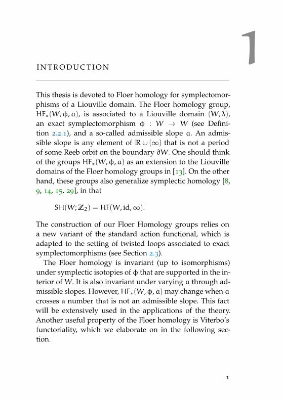
Definition 4.1.1. Let 0 < a < b be such that a is admissiblewith respect to W2 and b is admissible with respect to W1,and let b0 be the greatest period of some Reeb orbit on∂W1 that is smaller than b. The set Hstair(φ,W1,W2,a,b)is defined to be the set of (time-independent) HamiltoniansH : W2 → R having the following property. There existpositive real numbers δ1, δ2, δ3,A,B,C ∈ R+ and functions

h1 : [δ1, 2δ1]→ R,

h2 : [1− δ2, 1]→ R,

h3 : [1+ δ3, 1+ 2δ3]→ R,

such that

1. φ is compactly supported in the interior of Wδ1 ,

2. supp∈W1

∣∣Fφ(p)∣∣ < A,

40

3. h1 and h3 are convex and strictly increasing,

4. h2 is concave, strictly increasing, and h2(r) > rb0 forall r ∈ [1− δ2, 1],

and such that

H(p) = for

−A p ∈Wδ1 ,

h1(r) p = (x, r) ∈ [δ1, 2δ1)× ∂W1,

b(r− 2δ1) p = (x, r) ∈ [2δ1, 1− δ2)× ∂W1,

h2(r) p = (x, r) ∈ [1− δ2, 1]× ∂W1,

B p ∈W1+δ32 \W1,

h3(r) p = (x, r) ∈ (1+ δ3, 1+ 2δ3)× ∂W2,

ar+C p = (x, r) ∈ [1+ 2δ3,∞)× ∂W2.

A typical element of Hstair(φ,W1,W2,a,b) is shown inFigure 1.

Definition 4.1.2. Let W be a Liouville domain, and let φ :

W → W be a diffeomorphism. The support radius ρ(W,φ)of φ is defined by

ρ(W,φ) := infr ∈ R+ : suppφ ⊂Wr

.

Lemma 4.1.3. Let a,b, and b0 be as in Definition 4.1.1. If

C(W1,φ) < min b− b0,b− a ,

where

C(W1,φ) := 2max

supp∈W1

∣∣Fφ(p)∣∣ , ρ(φ,W1, λ)

, (4.1.27)

then the set Hstair(φ,W1,W2,a,b) is not empty.

41

Wδ11

W2δ11

W1−δ21

W1

W2

Wδ32

W2δ32

W2

−A

B H

Figure 1: A stair-like Hamiltonian

42

Proof. The constants δ1, δ2, δ2,A,B,C from Definition 4.1.1are chosen in the following way and the following order.

• Choose

A ∈(C(W1,φ)

2,

minb− b0,b− a2

),

• choose δ1 ∈(Ab , minb−b0,b−a

2b

),

• choose δ2 ∈(0, 1− 2bδ1

b−b0

),

• choose B ∈ (maxa,b0,b− 2bδ1 − bδ2,b− 2bδ1),

• choose δ3 ∈(0, B−aa

),

• choose C ∈ (max0,B− a(1+ 2δ3),B− a(1+ δ3)).

It follows that the following inequalities hold

0 < −A− (2bδ1) − bδ1 < bδ1, (4.1.28)

0 < B− (−2bδ1) − b(1− δ2) < bδ2, (4.1.29)

b(1− δ2) + (−2bδ1) > (1− δ2)b0, (4.1.30)

B > b0, (4.1.31)

0 < B−C− a(1+ δ3) < aδ3. (4.1.32)

Due to Lemma A.0.1 and Lemma A.0.2, (4.1.28) implies thath1 exists, (4.1.29), (4.1.30), (4.1.31) imply that h2 exists, and(4.1.32) implies that h3 exists. This finishes the proof.

Lemma 4.1.4. Let φ,a,b,H, δ1, δ2, δ3,A,B,C be as in Defini-tion 4.1.1. The ranges of the action functional Aφ,H when eval-uated on φ-twisted Hamiltonian orbits contained in different re-gions in W2 are given in the following table.

43

region Aφ,H ∈Wδ11 [A−

∥∥Fφ∥∥ ,A+∥∥Fφ∥∥]

(δ1, 2δ1)× ∂W1 (A, 2bδ1)

(1− δ2, 1)× ∂W1 (−B, 0)

W1+δ32 \ intW1 −B

(1+ δ3, 1+ 2δ3)× ∂W2 (−B,−C)

Note that each φ-twisted orbit of H is contained in one of theseregions.

Proof. We will prove the statement only for the region

(1− δ2, 1)× ∂W1.

For the other regions, the proof is similar and even moredirect.

The symplectomorphism φ is equal to the identity in(1− δ2, 1)×∂W1. Therefore, the twisted Hamiltonian orbitscoincide with Hamiltonian loops. Additionally, due to theform of the Hamiltonian H in this region, they can be ex-plicitly described in terms of periodic Reeb orbits on ∂W1.Each 1-periodic Hamiltonian orbit in (1 − δ2, 1) × ∂W1 isgiven by

t 7→(r0,γ(−h ′2(r0)t)

)(4.1.33)

where γ : R → ∂W1 is a h ′2(r0)-periodic Reeb orbit. Theaction of (4.1.33) is equal to

r0h′2(r0) − h2(r0).

Consider the function

f : [1− δ2, 1]→ R : r 7→ rh ′2(r) − h2(r).

44

Since f ′(r) = rh ′′2 (r) 6 0, f is decreasing. Hence the actionof a 1-periodic Hamiltonian orbit in (1− δ2, 1)×∂W1 lies inthe interval [f(1), f(r1)] = (−B, f(r1)), where r1 ∈ (1− δ2, 1)is the smallest number such that h ′2(r1) is a period of someReeb orbit on ∂W1. Since h ′2 is continuous and decreasing(h2 is concave), we get h ′2(r1) = b0. Therefore,

f(r1) = r1b0 − h2(r1) < 0

(because, by definition, h2(r) > rb0 for all r ∈ [1− δ2, 1]).This finishes the proof.

Proposition 4.1.5. Let φ : W1 → W1 be an exact symplecto-morphism and let φt : W1 → W1 be the isotopy of exact sym-plectomorphisms given by

φt :=(ψλt)−1 φ ψλt ,

where ψλt : W1 → W1 is the Liouville flow. Then,

Fφt = e−tFφ ψλt

and

ρ(φt,W1, λ) = e−tρ(φ,W1, λ).

Consequently, C(W1,φt) = e−tC(W1,φ).

Proof. Denote ψλt by ψt for simplicity. The Cartan formulaimplies ψ∗tλ = etλ and

(ψ−1t

)∗λ = e−tλ. Therefore

dFφt = φ∗tλ− λ

=(ψ−1t φ ψt

)∗λ− λ

= ψ∗tφ∗ (ψ−1

t

)∗λ− λ

= e−tψ∗t (φ∗λ− λ)

= e−td(Fφ ψt).

45

Hence Fφt = e−tFφ ψt. Since

suppφt ⊂Wr ⇐⇒ suppφ ⊂Wetr,

the equality ρ(W1,φt) = e−tρ(W1,φ) holds.

4.2 construction of the transfer morphism

Definition 4.2.1. Let a and b be as in Definition 4.1.1.Transfer data for (φ,W1,W2,a,b) is Floer data (H, J) for(φ : W2 → W2,b) satisfying the following. There exists aHamiltonian H ∈ Hstair(φ,W1,W2,a,b) such that H = H in[2δ1, 1− δ2]× ∂W1 and [1+ 2δ3,∞)× ∂W2, and such thatthe action functional is positive at twisted Hamiltonian or-bits in W2δ1

1 and negative at the other twisted orbits (thisholds for H that is C2-close to H). Additionally,

dr Jt = −λ

in [2δ1, 1− δ2]× ∂W1.

Lemma 4.2.2. Let (H, J) be a regular transfer data for(φ,W1,W2,a,b). By definition, there exist δ1, δ2 ∈ (0, 1) suchthat 2δ1 + δ2 < 1 and Ht(x, r) = b(r − 2δ1) for all (r, x) ∈[2δ1, 1− δ2)× ∂W1. Let Gt : W1 → R be a Hamiltonian de-fined by

Gt(p) :=

Ht(p) for p ∈W1−δ2

1

b(r− 2δ1) for p ∈ [2δ1,∞)× ∂W1.

Then,

HF∗(W1,φ,G, J) = HF>0∗ (W2,φ,H, J).

46

Proof. The generators of the chain complexesCF∗(W1,φ,G, J) and CF

>0∗ (W2,φ,H, J) coincide. There-

fore it is enough to prove the following. The solutions

u : R2 → W2, φ(u(s, t+ 1)) = u(s, t)

of the Floer equation which connect two Hamiltoniantwisted orbits in W1 satisfy u

(R2)⊂ W1. This follows

from the part a) of Theorem 4.5 in [16]. See also [16, Propo-sition 4.4].

We are going to define the transfer morphism in coupleof steps. Definition 4.2.3 defines it for positive slopes withadditional technical conditions. Definition 4.2.4 and Defini-tion 4.2.7 eliminate the technical conditions. And, finally,Proposition 4.2.6 extends the transfer morphism to the caseof infinite slopes.

Definition 4.2.3. Let a,b ∈ R+ be positive real numberssuch that a and b are admissible with respect to W2 andW1, respectively, and such that a < b. Let b0 be the greatestperiod of some Reeb orbit on ∂W1 that is smaller than b.Assume

C(W1,φ) < min b− b0,b− a .

The transfer morphism is defined to be the map

HF∗(W2,φ,a)→ HF∗(W1,φ,b),

induced by the natural map of chain complexes

CF∗(W2,φ,H, J)→ CF>0∗ (W2,φ,H, J),

where (H, J) is regular Transfer data for (φ,W1,W2,a,b).

47

Definition 4.2.4. Let a ∈ R+ be admissible with respectto W2, and let b ∈ R+ be admissible with respect to W1.Assume a < b. The transfer morphism is defined as thecomposition

HF∗(W2,φ,a) HF∗(W1,φ,b)

HF∗(W2,φ1,a) HF∗(W1,φ1,b).

I(φt)

T

I(φt)−1

Here,

φt := (ψλct)−1 φ ψλct, t ∈ [0, 1],

for c ∈ R+ such that

C(W1,φ1) < minb− b0,b− a,

and T is the transfer morphism of Definition 4.2.3.

Lemma 4.2.5. In the situation of Definition 4.2.4, the transfermorphism does not depend on the choice of c.

Proof. Let c1 and c2 be positive real numbers such that

C(W1,φi) < minb− b0,b− a, i ∈ 1, 2,

where

φi := (ψλci)−1 φ ψλci , i ∈ 1, 2.

It is enough to prove that the diagram

HF∗(W2,φ1,a) HF∗(W1,φ1,b)

HF∗(W2,φ,a) HF∗(W1,φ,b)

HF∗(W2,φ2,a) HF∗(W1,φ2,b)

48

commutes, where the vertical arrows stand for the iso-morphisms induced by symplectic isotopies. These isomor-phisms, as it follows from their definition in Section 3.4, co-incide with naturality isomorphisms with respect to someHamiltonians that are compactly supported in the interiorof W1. Hence, it is enough to prove that the diagram

HF(W2,φ1,a) HF(W1,φ1,b)

HF(W2,φ2,a) HF(W1,φ2,b)

N(H) N(K)

commutes, where H,K : W2 → R are compactly supportedin the interior of W1. This follows from the following fact.The naturality with respect to a Hamiltonian W2 → R

that is compactly supported in the interior of W1 convertstransfer data for (φ1,W1,W2,a,b) into transfer data for(φ2,W1,W2,a,b).

Proposition 4.2.6. The diagram

HF∗(W2,φ,a) HF∗(W1,φ,b)

HF∗(W2,φ,a ′) HF∗(W1,φ,b ′),

consisting of transfer morphisms and continuation maps, com-mutes whenever a,b,a ′,b ′ ∈ R+ are such that all the maps inthe diagram are well defined.

Proof of Theorem 1.1.1. The proof follows from the proof ofProposition 4.7 in [16].

Definition 4.2.7. Let a ∈ R+ be admissible with respect toboth W1 and W2. Let ε > 0 be a positive number such that

49

the elements of [a,a+ ε] are all admissible with respect toW1. The transfer morphism

HF∗(W2,φ,a)→ HF∗(W1,φ,a)

is defined to be the composition of the transfer morphism

HF∗(W2,φ,a)→ HF∗(W1,φ,a+ ε)

of Definition 4.2.4 and the inverse of the continuation map

Φ−1 : HF∗(W1,φ,a+ ε)→ HF∗(W1,φ,a).

Lemma 4.2.8. The transfer morphism of Definition 4.2.7 is welldefined and does not depend on the choice of ε.

Proof. Lemma A.0.3 implies that ε from Definition 4.2.7 ex-ists. Due to Proposition 3.2.1, the continuation map

Φ : HF∗(W1,φ,a)→ HF∗(W1,φ,a+ ε)

is an isomorphism. Hence, its inverse Φ−1 is well defined.Independence of the choice of ε follows from Proposi-tion 4.2.6.

Proposition 4.2.6 enables us to extend the transfer mor-phism to the case of infinite slopes. The proposition is stilltrue after the extensions of the transfer morphism.

50

5A P P L I C AT I O N S

5.1 the symplectic mapping class group

Let (W, λ) be a Liouville domain. The group of all symplec-tomorphisms W → W that are compactly supported in theinterior of W is denoted by Sympc(W,dλ).

Definition 5.1.1. The symplectic mapping class group ofa Liouville domain (W, λ) is defined to be the groupπ0 Sympc(W,dλ). In other words, it is the group of sym-plectomorphisms up to symplectic isotopies. (Both the sym-plectomorphisms and the isotopies are assumed to be com-pactly supported in the interior of W.) The elements of thesymplectic mapping class group are called symplectic map-ping classes.

The Floer homology is not defined for an arbitrary sym-plectomorphism of a Liouville domain. Nevertheless, thesymplectic mapping class group is investigable by the Floerhomology for exact symplectomorphisms. This is due to thefollowing lemma.

Lemma 5.1.2 (Giroux). For any Liouville domain (W, λ), theinclusion

j : Sympc(W, λ/d)→ Sympc(W,dλ)

is a homotopy equivalence.

51

Proof (following [6]). Denote the symplectic form dλ by ω.We construct a homotopy inverse of j as follows. LetYφ, φ ∈ Sympc(W,ω) be a vector field on W defined by

λ−φ∗λ = ω(Yφ, ·

).

Since Yφ is compactly supported in W − ∂W, its flow ψφt is

well defined. We denote by T the map

Sympc(W,ω)→ Sympc(W, λ/d) : φ 7→ φ ψφ1 .

First, we prove that T is well defined, i.e. that

T(φ) ∈ Sympc(W, λ/d).

Note that ψφt =: ψt is a symplectomorphism for all realt, and that it preserves the form λ − φ∗λ. Using Cartan’sformula, we get

d

dt(ψ∗tλ) = ψ

∗t

(Yφydλ+ dYφyλ

)= ψ∗t

(λ−φ∗λ+ d

(λ(Yφ)))

= λ−φ∗λ+ d(λ(Yφ)ψt

).

Hence

ψ∗tλ− λ = (λ−φ∗λ) t+ d

(∫t0

λ(Yφ)ψsds

). (5.1.34)

This implies that

(φ ψ1)∗λ− λ = ψ∗1φ∗λ−ψ∗1λ+ψ

∗1λ− λ

= ψ∗1 (φ∗λ− λ) +ψ∗1λ− λ

= ψ∗1λ− λ− (λ−φ∗λ)

(5.1.35)

is an exact form.

52

Now, we prove that j T and T j are homotopic to theidentity. The homotopies are given by

[0, 1]× Sympc(W,ω)→ Sympc(W,ω)

(t,φ) 7→ φ ψφt ,

and

[0, 1]× Sympc(W, λ/d)→ Sympc(W, λ/d)

(t,φ) 7→ φ ψφt .

In what follows, we check that the latter is well defined.Similarly as in (5.1.35), we get(

φ ψφt)∗λ− λ =

((ψφt

)∗λ− λ

)+ (φ∗λ− λ) .

The both forms in the brackets (on the right-hand side ofthe equation above) are exact: the latter because of φ ∈Sympc(W, λ/d), and the former because of (5.1.34) in ad-dition.

5.2 the fibered dehn twist

This section is devoted to a construction of an interestingclass of exact symplectomorphisms. These symplectomor-phisms are defined on Liouville domains having periodicReeb flow on their boundaries.

Definition 5.2.1. [6, 24]. Let (W, λ) be a Liouville domainwith 1-periodic Reeb flow on the boundary. Let v : R → R

be a smooth function which is equal to 0 on (−∞, 0) and to−1 on (0.95,+∞). The (right-handed) fibered Dehn twistis an element τ of Sympc(W, λ/d) defined by

τ(p) =

(r,σv(r)(x)

)for p = (r, x) ∈ R+ × ∂W,

p otherwise,

53

where σt : ∂W → ∂W stands for the Reeb flow. The isotopyclass of τ does not depend on the choice of v.

Remark 5.2.2. The fibered Dehn twist of Definition 5.2.1, isa time-1 map of the Hamiltonian K : W → R

K(p) :=

−V(r) for p = (r, x) ∈ R+ × ∂W,

0 otherwise.

Here, V : R→ R is the unique primitive of v equal to 0 near0. Note that

K(x, r) = r−∫10

v(t)dt− 1

near infinity.

The disk-cotangent bundle D∗Sn of the sphere Sn withthe standard Riemannian metric (rescaled by 2π) is an ex-ample of a Liouville domain that satisfies the conditionsfrom Definition 5.2.1. The fibered Dehn twist for D∗Sn rep-resents the same symplectic mapping class as the squareof the so-called generalized Dehn twist [4, 22], which wasconsidered by Seidel in his thesis.

Given a Lagrangian sphere L in a symplectic manifoldW, one can use the fibered Dehn twist (or the generalizedDehn twist) on D∗Sn to construct a symplectomorphism ofW that is supported in a neighbourhood of L. This is dueto the Weinstein theorem, which guarantees the existenceof a neighbourhood of L in W that is symplectomorphicto D∗Sn. Note, however, that the symplectomorphism be-tween D∗Sn and the neighbourhood is not unique. Some-times, different identifications of the neighbourhood withD∗Sn lead to symplectomorphisms of W that are not sym-plectically isotopic to each other [11, Theorem A].

54

We describe below a long exact sequence due to Giroux[6] which provides further examples of symplectic mappingclasses. The fibered Dehn twist can be seen as a special caseof this construction (see Proposition 5.2.6).

Let (W, λ) be a Liouville domain. We denote bySymp(W, λ/d) the group of symplectomorphisms φ : W →W such that the 1-form φ∗λ− λ is exact and compactly sup-ported. The elements of the group Symp(W, λ/d) are notnecessarily compactly supported.

Lemma 5.2.3. Let (W, λ) be a Liouville domain, and let φ ∈Symp(W, λ/d). Then, there is a contactomorphism φ∂ : ∂W →∂W and a function f : ∂W → R+ such that

φ∗∂β = fβ

and

φ(r, x) =(r

f(x),φ∂(x)

)for all x ∈ ∂W and all r ∈ R+ large enough.

Proof. There exists r0 ∈ R+ such that the restriction of φ to(r0,∞)× ∂W is a λ-preserving embedding

(r0,∞)× ∂W → R+ × ∂W.

Let

φ(r, x) = (g(r, x),σ(r, x)) ∈ R+ × ∂W

for (r, x) ∈ (r0,∞)× ∂W. Since φ preserves λ and ω, it pre-serves the vector field Xλ = r∂r (because Xλ is characterizedby the relation Xλyω = λ). Thus, φ commutes with the flowof r∂r, i.e.(

g(etr, x

),σ(etr, x

))=(etg (r, x) ,σ (r, x)

).

55

This implies that σ(r, x) does not depend on r. The mapσ(r, ·), denoted by φ∂, is a contactomorphism, because

rβ = φ∗(rβ) = g(r, x)φ∗∂β

implies

φ∗∂β =r

g(r, x)β

and rg(r,x) is a positive function. Another consequence is

that rg(r,x) =: f(x) does not depend on r. Hence, the proof

is finished.

Definition 5.2.4. In view of Lemma 5.2.3, one can asso-ciate a contactomorphism φ∂ : ∂W → ∂W to every symplec-tomorphism φ ∈ Symp(W, λ/d). This gives rise to the ho-momorphism

Θ : Symp(W, λ/d

)→ Cont (∂W) : φ 7→ φ∂,

which we call the ideal restriction map.

Let Symp(W, λ/d) be the group of symplectomorphisms

ϕ : W → W

such that ϕ∗λ− λ = dF for a function F : W → R compactlysupported in W − ∂W.

Proposition 5.2.5. The ideal restriction map of Definition 5.2.4

Θ : Symp(W, λ/d)→ Cont(∂W)

is a Serre fibration with fibre over the identity equal to the groupSympc(W, λ/d) of all exact symplectomorphisms of W.

56

Proof (following [6]). By definition, a Serre fibration is a con-tinuous map that satisfies the homotopy lifting property forcubes, Im. To prove the proposition, we should show thatfor any homotopy

f :I× Im → Cont(∂W)

(t,y) 7→ ft(y)

and for any lift f0 of f0 (i.e. Θ f0 = f0), there exists ahomotopy

f : I× Im → Symp(W, λ/d)

such that Θ f = f. Let Kt(y) : R+ × ∂W be the contactHamiltonian generating the path

t 7→ ft(y) ∈ Cont(∂W)

of contactomorphisms, i.e. Kt(y) is an R+-equivariantHamiltonian on the symplectization R+×∂W such that thefollowing diagram commutes

R+ × ∂W R+ × ∂W

∂W ∂W.

ψK(y)t f0

pr2 pr2ft(y)

Let χ : W → [0, 1] be a cut-off function that is equal to 0 onW

13 and to 1 outside W

23 . Denote by Gt(y) : W → R the

Hamiltonian defined by

Gt(y)(p) := χ(p)Kt(y)(p), p ∈W.

Now, we can take

f(t,y) := ψG(p)t f0.

57

This proves that Θ is a Serre fibration. The fibre is equal to

Θ−1(id) = Sympc(W, λ/d).

By Proposition 5.2.5, there is a homotopy long exact se-quence

...

πk Sympc(W, λ/d) πk−1 Sympc(W, λ/d)

πk Symp(W, λ/d)...

πkCont(∂W)

∆ (5.2.36)

In particular, there is a connecting homomorphism

∆ : π1Cont(∂W)→ π0 Sympc(W, λ/d). (5.2.37)

In view of Lemma 5.1.2, the inclusion

Sympc(W, λ/d)→ Sympc(W,dλ)

induces isomorphism on homotopy groups, so that thegroups πi Sympc(W, λ/d) in (5.2.36) and (5.2.37) can be re-placed by πi Sympc(W,dλ).

Proposition 5.2.6. Let (W, λ) be a Liouville domain with 1-periodic Reeb flow σt : ∂W → ∂W on the boundary. Then, theimage ∆([σ]) of the class [σ] ∈ π1Cont(∂W) under the connect-ing homomorphism ∆ is represented by the fibered Dehn twist.

58

Proof. The proposition follows from Lemma 5.2.7 (appliedin the case of Yt being the Reeb vector field), Lemma 5.2.8and Remark 5.2.2.

Lemma 5.2.7. Let (W, λ) be a Liouville domain. We denote by αthe induced contact form on the boundary. Let σt : ∂W → ∂W

be a 1-periodic family of contactomorphisms generated by a vec-tor field Yt. Then the family σt determines an element ofπ1Cont(∂W) whose image under the connecting homomorphism∆ can be represented by the time-1 map of a (non-compactly sup-ported) Hamiltonian W → R that is equal to −rα(Yt) near in-finity.

Proof. The element in π1Cont(∂W) determined by σt isdenoted (by a slight abuse of notation) by [σ]. By definition,∆([σ]) is equal to [ψ1] ∈ π0 Sympc(W,dλ), where ψt is apath in Symp(W, λ/d) such that Θ(ψt) = σt (see Defini-tion 5.2.4). Let χ : R+ → R be a smooth function equal to 0near 0 and 1 on [1,∞). We can choose ψt from above to beψHt where H : W → R is the Hamiltonian that is equal to

(r, x) 7→ −χ(r)rα(Yt)

on R+ × ∂W and 0 elsewhere. This finishes the proof.

Lemma 5.2.8. Let (W, λ) be a Liouville domain, and let Ht andKt be two Hamiltonians on W that are equal near infinity andwhose flows are well-defined for all times. If the maps ψH1 andψK1 are compactly supported in W − ∂W, then they represent thesame class in π0 Sympc(W,dλ).

Proof. The HamiltonianH#K (see page 33) is compactly sup-ported and generates the Hamiltonian isotopy ψHt

(ψKt)−1

(compactly supported as well). This isotopy, however, maynot be supported in the interior of W for all times. Let φλt

59

be the family of diffeomorphisms of W that is generatedby the Liouville vector field Xλ. The diffeomorphism φλt isnot a symplectomorphism (except for t = 0), however ifwe conjugate a symplectomorphism by it we get a symplec-tomorphism. Since the isotopy ψHt

(ψKt)−1 is compactly

supported, there exists s ∈ R+ such that(φλs)−1 ψHt (ψK)−1 φλs

is compactly supported in the interior of W. In particular,the maps

(φλs)−1 ψH1 φλs and

(φλs)−1 ψK1 φλs represent

the same class in π0 Sympc(W,dλ). Note that(φλt)−1 ψH1 φλt ∈ Sympc(W,dλ)

for all t ∈ R+. Hence(φλs)−1 ψH1 φλs and ψH1 repre-

sent the same class in π0 Sympc(W,dλ). Similarly, the sameholds for

(φλs)−1 ψK1 φλs and ψK1 , and the proof is fin-

ished.

5.3 detecting nontrivial mapping classes

Theorem 5.3.1. Let (W, λ) be a Liouville domain such that theReeb flow on the boundary ∂W is 1-periodic, and let a ∈ R bean admissible slope. If the fibered Dehn twist represents a class oforder ` ∈N in π0 Sympc(W,dλ), then

HF(W, id,a) ∼= HF(W, id,a+ `). (5.3.38)

Proof. Remark 5.2.2 implies that the `-th power of thefibered Dehn twist τ` is the time-1 map of a HamiltonianK : W → R that is equal to `r near infinity. The naturalityprovides us with the isomorphism (see Proposition 3.3.4)

N(K) : HF(W, id,a+ `)∼=→ HF(W, τ`,a) (5.3.39)

60

for all admissible a ∈ R. On the other hand, if we as-sume that τ` represents trivial class in π0 Sympc(W,dλ),by Lemma 5.1.2, it represents the trivial class inSympc(W, λ/d) as well. Theorem 3.4.3 implies

HF(W, id,a) ∼= HF(W, τ`,a). (5.3.40)

From (5.3.39) and (5.3.40), we get

HF(W, id,a) ∼= HF(W, id,a+ `). (5.3.41)

(In general, the isomorphism (5.3.41) preserves neither thegrading nor the class in π0Ωφ.)

Remark 5.3.2. Strictly speaking, the construction of thegroups HF∗(W,φ,a) for φ 6= id was not necessary for theproof of Theorem 5.3.1. In this remark, we rewrite the proofof Theorem 5.3.1 without mentioning HF∗(W,φ,a) for φ 6=id . Let K : W → R be a Hamiltonian equal to `r near infinitysuch that ψK1 = τ`, and let Gt : W → R be a compactly sup-ported Hamiltonian such that Gt+1 = Gt and ψG1 = τ`. TheHamiltonian G exists because [τ`] = 1 ∈ π0 Sympc(W, λ/d)and because of Lemma 3.4.2. Consider the HamiltonianG#K. It has the slope equal to −` and generates the isotopyψGt (ψKt )−1. In particular, its time-1 map is equal to theidentity. Now, the naturality with respect to this Hamilto-nian provides the isomorphism (5.3.41).

Corollary 5.3.3. Let (W, λ) be as in Theorem 5.3.1. If

dimH(W; Z2) < dimSH(W; Z2), (5.3.42)

then the fibered Dehn twist represents a class of infinite order inπ0 Sympc(W,dλ). Here, dimH(W; Z2) stands for the sum ofBetti numbers rather than the dimension of the homology groupof a particular degree.

61

Proof. Assume, by contradiction, that the fibered Dehntwist represents a class of order ` ∈ N in π0 Sympc(W,dλ)(and, equivalently, in π0 Sympc(W, λ/d)). Then Theo-rem 5.3.1 implies

HF(W, id,a) ∼= HF(W, id,a+ `)

for all admissible a ∈ R. In particular,

HF(W, id,k`− ε) ∼= HF(W, id,−ε) ∼= H(W; Z2),

for k ∈ Z and ε > 0 small enough (see also Example 2.7.7).It follows that

dimHF(W, id,k`− ε) = dimH(W; Z2). (5.3.43)

Since

SH(W; Z2) = HF(W, id,∞) = lim−→a

HF(W, id,a)

has dimension greater than or equal to

d := dimH(W, Z2) + 1,

there exist elements αj ∈ HF(W, id,aj), j ∈ 1, . . . ,d suchthat

ι(α1), . . . , ι(αd) ∈ SH(W; Z2)

are linearly independent. Here, ι stands for the homomor-phisms

ι : HF(W, id,a)→ lim−→a

HF(W, id,a).

Let ε > 0 be small enough, and let k ∈N be such that

k`− ε > maxa1, . . . ,ad.

62

Then the images of α1, . . . ,αd under the continuation maps

HF(W, id,aj)→ HF(W, id,k`− ε), j ∈ 1, . . . ,d

are linearly independent. However, this leads to contradic-tion, because of (5.3.43) and d > dimH(W; Z2).

Definition 5.3.4. Let m ∈ N be a natural number. A Zm-graded vector space V∗ is called symmetric if there existsk ∈ Zm such that

Vk−j ∼= Vj

for all j ∈ Zm.

Corollary 5.3.5. Let (W, λ) be a Liouville domain, let o ∈π0Ωid be the class of contractible loops, and let N be the min-imal Chern number No (see page 14). Assume the Reeb flowinduces a free circle action on the boundary ∂W. If the ho-mology H∗(W; Z2) rolled up modulo 2N is not symmetric,then the fibered Dehn twist represents a nontrivial class inπ0 Sympc(W,dλ).

Proof. Assume the contrary, i.e. that the fibered Dehn twistrepresents the trivial class in π0 Sympc(W,dλ). Let 1 > ε >0. Theorem 5.3.1 implies

HF(W, id,−ε) ∼= HF(W, id, 1− ε).

This isomorphism preserves neither the grading nor theclass in π0Ωid. However, it preserves the relative grading.Hence there exist a class o ′ ∈ π0Ωid and c ∈ Z2N such that

HF∗(W, id,−ε,o) ∼= HF∗+c(W, id, 1− ε,o ′). (5.3.44)

63

Since ε ∈ (−1, 0), 1 − ε ∈ (0, 1) and numbers in (−1, 0) ∪(0, 1) are all admissible, we get (by Proposition 3.2.1 andExample 2.7.7)

HF∗(W, id,−ε,o) ∼= H∗+n(W; Z2),

HF∗(W, id, 1− ε,o ′) ∼=

H∗+n(W,∂W; Z2) if o = o ′

0 if o 6= o ′.

The group H(W; Z2) is never 0. Hence (because of (5.3.44)),o = o ′ and

H∗(W; Z2) ∼= H∗+c(W,∂W; Z2).

By Poincaré duality

H∗(W,∂W; Z2) ∼= H2n−∗(W; Z2).

Since we are working with field coefficients, we have

H2n−∗(W, Z2) ∼= Hom(H2n−∗(W; Z2), Z2)

∼= H2n−∗(W; Z2).

Therefore

H2n−c−∗(W; Z2) ∼= H∗(W; Z2).

This contradicts the fact that H∗(W; Z2) is not symmetric.

Corollary 5.3.6. Let (W, λ) be as in Theorem 5.3.1. Assume thatthe Reeb flow induces a free circle action on ∂W, and that the firstChern class c1(W) vanishes. If the homology H∗(W; Z2) is notsymmetric, then the fibered Dehn twist represents a nontrivialclass in π0 Sympc(W,dλ).

Proof. The corollary is a special case of Corollary 5.3.5 (thecase in which N =∞).

64

5.4 examples

Example 5.4.1. Let (Q,g) be a closed Riemannian manifold.We denote by D∗Q and S∗Q the disk cotangent bundle andthe unit cotangent bundle of Q, respectively. The standardLiouville form λcan on T∗Q equips D∗Q with the structureof a Liouville domain. The Reeb flow on S∗Q coincideswith the geodesic flow of Q under the obvious identifica-tion of tangent and cotangent bundles of Q. It is periodicif, and only if, the geodesics of (Q,g) are all closed. Exam-ples of Riemannian manifolds with all geodesics periodicare spheres Sm, complex and quaternionic projective spacesCPm and HPm, and the Cayley plane (octonionic projectiveplane) CaP2 with the standard metrics.

Assume (Q,g) is one of these manifolds. We can rescaleg so that the Reeb flow on S∗Q is 1-periodic. By a theoremof Viterbo (see Theorem 5.4.2 below), the symplectic homol-ogy SH∗(D∗Q; Z2) is isomorphic to the singular homologyH∗(ΛQ; Z2) of the free loop space of Q. The homology ofΛQ is explicitely computed in [31], and it turns out to be in-finite dimensional in Z2 coefficients. Hence Corollary 5.3.3implies that the corresponding fibered Dehn twist is of infi-nite order in π0 Sympc(D

∗Q,dλcan).

Theorem 5.4.2 (Viterbo). Let (Q,g) be a closed Riemannianmanifold, and let ΛQ be its free loop space. Then

SH∗(D∗Q; Z2) ∼= H∗(ΛQ; Z2).

Proof. Proofs can be found in [28], [1], [19], and [2].

Remark 5.4.3. Corollary 5.3.5 does not imply nontrivialityof the fibered Dehn twists for the Liouville domains con-sidered in Example 5.4.1. The reason is the following. Let

65

(Q,g) be as in Example 5.4.1. The disk cotangent bundleD∗Q is homotopic to Q, which is a closed manifold, andtherefore (by Poincaré duality), the homology H∗(D∗Q; Z2)

is symmetric.

Remark 5.4.4. The fibered Dehn twists on D∗S2 and D∗S6

are smoothly isotopic to the identity relative to the bound-ary (see Lemma 6.3 in [23] and also Lemma 10.2 in [5]).The same is true for D∗CPm, m ∈ N [24, Proposition 4.6].On the other hand, the fibered Dehn twist on D∗Sm form 6∈ 2, 6 is not even smoothly isotopic to the identityrelative to the boundary (see, for example, Lemma 10.1in [5]). Interestingly, the only manifolds among Sm andCPm, m ∈ N, admitting almost complex structures areS2, S6 and CPm, m ∈ N. This is not a coincidence (seeProposition 5.4.5 below).

Proposition 5.4.5. Let (Q,g) be a Riemannian manifold whosegeodesics are all 1-periodic. Assume there exists an almost com-plex structure J on Q that preserves the norm of vectors in TQ.Then, the square of the fibered Dehn twist on D∗Q is smoothlyisotopic to the identity relative to the boundary.

It is an interesting question whether in the situation ofProposition 5.4.5 the fibered Dehn twist itself is smoothlyisotopic to the identity relative to the boundary.

Lemma 5.4.6. Let (Q,g) be as in Proposition 5.4.5. Denote bySQ ⊂ TQ the unit tangent bundle. Then the geodesic flow in-duces a loop of diffeomorphisms SQ → SQ whose square is con-tractible.

Proof. Let J be as in Proposition 5.4.5, and let γξ be theunique geodesic on Q such that γξ(0) = ξ ∈ TQ. The (re-striction of the) geodesic flow is given by

Ψt : SQ→ SQ : ξ 7→ γξ(t).

66

The antipodal map

SQ→ SQ : ξ 7→ −ξ

is isotopic to the identity via the isotopy

[0,π]× SQ→ SQ : (s, ξ) 7→ cos sξ+ sin sJξ.

Hence the loop

R/Z 3 t 7→ Ψt ∈ Diff(SQ)

is homotopic to the loop

t 7→ −Ψt(−·)

(Ψt is pre- and postcomposed by the antipodal map). Since

−Ψt(−ξ) = Ψ−1t (ξ), ξ ∈ SQ,

the loop t 7→ Ψt is homotopic to its inverse t 7→ Ψ−1t . There-

fore, the loop t 7→ Ψ2t is contractible.

Proof of Proposition 5.4.5. We take (W, λ) = (D∗Q, λcan). Thesquare of the fibered Dehn twist is given by

p 7→

(r,σ2v(r)(x)

)for p = (r, x) ∈ R+ × ∂W,

p otherwise,(5.4.45)

where σt is the Reeb flow on ∂W, and v : R → R is asmooth function that is equal to 0 on (−∞, 0) and −1 on(0.95,+∞). By Lemma 5.4.6, σ2 seen as a loop

R/Z→ Diff(∂W)

is homotopic to the constant loop t 7→ id . Let

Φs : R/Z→ Diff(∂W), s ∈ [0, 1]

67

be a homotopy between the loops t 7→ id and t 7→ σ2t . Anisotopy between (5.4.45) and the identity is given by

[0, 1]× W → W

(s,p) 7→

(r,Φsv(r)(x)

)for p = (r, x) ∈ R+ × ∂W,

p otherwise.

Albers and McLean found in [3] a large family of contactmanifolds such that every strong filling of them has infinitedimensional symplectic homology. It is an interesting ques-tion, in the view of Corollary 5.3.3, whether any of theirexact fillable examples has a periodic Reeb flow.

Example 5.4.7. Assume W is a higher-genus closed surfacewith an open disk removed. Since H∗(W; Z2) is not sym-metric, Corollary 5.3.5 implies that the fibered Dehn twistrepresents a nontrivial class in π0 Sympc(W). The FiberedDehn twist in this case is the Dehn twist along (a translateof) the boundary circle.

Example 5.4.8. Let V be a smooth degree d > 2 projectivehypersurface in CPm, m > 3, and let H be a hyperplanetransverse to V . By removing a neighbourhood of V ∩H inV , we get a Liouville domain W such that the Reeb flow in-duces a free circle action on its boundary ∂W. By [27], themanifoldW has the homotopy type of a bouquet of (m− 1)-spheres. Moreover, the number of the spheres is equal to(d− 1)m (see Theorem 1 and consequence (iii) on page 487

in [10]). Hence c1(W) = 0 and the homology H∗(W; Z2)

is not symmetric. Corollary 5.3.6 implies that the fiberedDehn twist of W is not symplectically isotopic to the iden-tity relative to the boundary. (See also Example 7.14 in [7].)

68

5.5 iterated ratio

Definition 5.5.1. Let φ :W →W be an exact symplectomor-phism of a Liouville domain W. The iterated ratio κ(W,φ)is defined to be the number

κ(W,φ) := lim supm→∞

dimHF(W,φm, ε)m

.

Here ε > 0 is small enough (smaller than any positive pe-riod of some Reeb orbit on ∂W).

It follows directly from the definition that κ(W, id) = 0.If the limit

limm→∞ dimHF(W,φm, ε)

m

exists, then

κ(W,φ`) = `κ(W,φ).

Remark 5.5.2. The iterated ratio is invariant under com-pactly supported symplectic isotopies. It measures the lin-ear growth rate of dimHF(W,φm, ε). There is yet anothersimilar invariant, the Floer theoretic entropy,

hFloer(W,φ) := lim supm→∞

log (dimHF(W,φm, ε))m

,

which measures the exponential growth rate ofdimHF(W,φm, ε). If W is a surface and φ an area-preserving diffeomorphism that has a pseudo-Anosovcomponent, then hFloer(W,φ) > 0 [26, page 167]. Conse-quently, κ(W,φ) is equal to infinity.

Theorem 5.5.3. Let (W2, λ) be a Liouville domain, let W1 ⊂W2 be a codimension-0 submanifold such that (W1, λ) is a Liou-ville domain in its own right, and let φ : W1 → W1 be an exactsymplectomorphism. Then, κ(W1,φ) = κ(W2,φ).

69

Proof of Theorem 5.5.3. Let ε > 0 be small. It is enough toprove that the number

|dimHF(W1,φm, ε) − dimHF(W2,φm, ε)|

is bounded (by a constant not depending on m). Let ψm :

W1 → W1 be an exact symplectomorphism that is isotopicto φm through exact symplectomorphisms, and such thatC(W1,ψm) < ε

2 (see (4.1.27) on page 41 for the defini-tion of C(W1,ψm)). Such a symplectomorphism exists foreach m ∈ N due to Proposition 4.1.5. Choose transfer data(Hm, Jm) for (ψm,W1,W2, ε2 , ε), such that Hm = H1 andJm = J1 on W2 \W1. The short exact sequence

0

CF<0∗ (W2,ψm,Hm, Jm)

CF∗(W2,ψm,Hm, Jm)

CF>0∗ (W2,ψm,Hm, Jm)

0

70

of chain complexes induces the long exact sequence in ho-mology

...

HF<0∗ (W2,ψm,Hm, Jm)

HF∗(W2,ψm,Hm, Jm)

HF>0∗ (W2,ψm,Hm, Jm)

...

By applying identifications as in Section 4.2, the long exactsequence is transformed into

...

HF<0∗ (W2,ψm,Hm, Jm)

HF∗(W2,ψm, ε2)

HF∗(W1,ψm, ε)

...

(5.5.46)

71

The chain complexes CF<0∗ (W2,ψm,Hm, Jm),m ∈ N aregenerated by twisted orbits contained in W2 \W1. In thisregion ψm = id and (Hm, Jm) = (H1, J1). Hence

CF<0∗ (W2,ψm,Hm, Jm), m ∈N

are generated by the same set of generators. This does notimply that

HF<0∗ (W2,ψm,Hm, Jm), m ∈N

are isomorphic, because the differentials may differ. How-ever,

dimHF<0∗ (W2,ψm,Hm, Jm) 6 dimCF<0∗ (W2,ψm,Hm, Jm)

= dimCF<0∗ (W2,ψ1,H1, J1),

and dimCF<0∗ (W2,ψ1,H1, J1) does not depend on m. Thelong exact sequence (5.5.46) implies∣∣∣dimHF

(W2,ψm,

ε

2

)− dimHF(W1,ψm, ε)

∣∣∣ < C,

where

C := 2dimCF<0(W2,ψ1,H1, J1).

Finally, note that

HF(W2,ψm,

ε

2

)∼= HF

(W2,φm,

ε

2

)∼= HF(W2,φm, ε),

and

HF(W1,ψm, ε) ∼= HF(W1,φm, ε).

This finishes the proof.

72

The following proposition shows that symplectomor-phisms which are supported in the cylindrical part of aLiouville domain have finite iterated ratio.

Proposition 5.5.4. Let (W, λ) be a Liouville domain, and letφ : W → W be an exact symplectomorphism that is compactlysupported in (0, 1)× ∂W. Then

κ(W,φ) <∞.

Proof. The idea of the proof is the following. We constructan exact symplectomorphism ψm :W →W that is symplec-tically isotopic to φm relative to the boundary, and suchthat it consists of m “copies” of φ with disjoint supports.By choosing a suitable Hamiltonian, one can ensure thateach “copy” contributes the same number of generatorsto the Floer chain complex. Since the number of “copies”grows linearly with respect to m, the iterated ratio has tobe smaller than the number of generators furnished by asingle “copy.”

Now, we implement the idea rigorously. By the assump-tion, there exists δ ∈

(0, 12

)such that φ is compactly sup-

ported in (2δ, 1)× ∂W. Let ε > 0 be small, and let Ht : W →R be a Hamiltonian equal to

(r, x) 7→ εr

on (δ, 2δ)× ∂W ∪ (1,∞)× ∂W such that

Ht+1 = Ht φ,

and such that

det(d(φ ψH1 )(x) − id

)6= 0

for all fixed points x of φ ψH1 . The non-degeneracy con-dition implies that there are finitely many Hamiltonian

73

twisted orbits. We denote by A and B the numbers of suchorbits in Wδ and (2δ, 1)× ∂W, respectively.

Fix m ∈ N. Denote by ϕ0 : W → W the symplectomor-phism

ϕ0 := ψλT φ

(ψλT)−1

,

where

T := (m− 1) ln δ−m ln(1+ δ),

and ψλt is the Liouville flow. Let ϕj, j ∈ 1, . . . ,m− 1 bethe symplectomorphism given by

ϕj := ψλjc ϕ0

(ψλjc)−1

,

where c := ln(1+ δ) − ln δ. Similarly, denote

H0t := Ht (ψλT)−1

,

Hjt := H

0t (ψλjc)−1

, j ∈ 1, . . . ,m− 1.

The symplectomorphisms ϕ0,ϕ1, . . . ,ϕm−1 are all sym-plectically isotopic to φ relative to the boundary, and theyare compactly supported in

(r0, r0ec)× ∂W,(r0e

c, e0e2c)× ∂W,

. . . ,(r0e

(m−1)c, r0emc)× ∂W,

(5.5.47)

respectively. Here,

r0 :=δm

(1+ δ)m,

74

and c is as above. (It follows that r0emc = 1 and con-sequently the sets (5.5.47) are all subsets of W. Hence,ϕj is compactly supported in the interior of W for allj ∈ 0, . . . ,m − 1.) Let ψm : W → W be the exact sym-plectomorphism

ψm := ϕ0 · · · ϕm−1,

and let Gt : W → R be the Hamiltonian defined by

Gt(p) :=

H0t(p) for p ∈Wr0 ,

Hjt(p) for p ∈ Sj, j ∈ 1, . . . ,m− 1

εr otherwise,

where

Sj :=(r0e

(j−1)c, r0ejc)× ∂W.

By construction, Gt has exactly A+mB Hamiltonian ψm-twisted loops, and they are all non-degenerate. This implies

dimHF(W,φm, ε) = dimHF(W,ψm, ε) 6 A+mB.

The first equality follows from φm being symplectically iso-topic to ψm relative to the boundary. Hence,

κ(W,φ) 6 limm→∞ A+mB

m= B <∞,

and the proof is finished.

5.6 iterated ratio of the fibered dehn twist on

D∗Sn

In this section, we compute the iterated ratio for thefibered Dehn twist τ : D∗Sn → D∗Sn [6, 24] of

75

the disk cotangent bundle of the sphere Sn endowedwith the standard Riemannian metric. The Floer homol-ogy HF(D∗Sn , τm , ε) , m ∈ N , is isomorphic (as a Z2-vector space) to HF(D∗Sn , id, 2πm + ε) . This followsfrom Proposition 3.3.4 and Remark 5.2.2. Hence

κ(D∗Sn , τ) = limm→∞ dim HF(D∗Sn , id, 2πm + ε)

m.

Proposition 5.6.1. Let m and n be positive integers, let ε be anelement of (0, 2π), and let D∗Sn be the disk cotangent bundleof Sn with respect to the standard Riemannian metric. Then, thevector space

HFk(D∗Sn, 2πm+ ε) (~)

has the following isomorphism type.

• If n = 2,

~ ∼=

Z2 for k ∈ 0, 1, 2m+ 1, 2m+ 2,

Z22 for k ∈N and 2 6 k 6 2m,

0 otherwise.

• If n > 2,

~ ∼=

Z2 for k ∈ Am,

0 otherwise,

where

Am := `(n− 1), `(n− 1)+n : ` ∈ Z & 0 6 ` 6 2m.

In particular,

dimHFk(D∗Sn, 2πm+ ε) = dimHFk(D

∗S2, 2πm+ ε)

= 4m+ 2.

76

Proof. We will consider only the case of S2. The proof forother cases is analogous and even simpler.The Reeb flow on S∗S2 := ∂D∗S2 is periodic with minimalperiod equal to 2π. Hence, there exists a homology longexact sequence

...

HFk(D∗S2, 2π`+ ε) HFk−1(D

∗S2, 2π`+ ε)

HFk(D∗S2, 2π(`+ 1) + ε)

...

Hk+∆`+1(S∗S2)

∆

(5.6.48)

where ` ∈ N ∪ 0, and ∆` is a shift in grading [21,Lemma 3.6]. The shift ∆` is equal to −(2`− 1) [18, Proposi-tion 5.12]. The long exact sequence (5.6.48) implies

HFk(D∗S2, 2π`+ ε)

∼=−→ HFk(D∗S2, 2π(`+ 1) + ε),

for k < 2`. Therefore

HFk(D∗S2, 2π`+ ε) ∼= SHk(D

∗S2), for k < 2`. (5.6.49)

77

We prove the proposition by induction. Using (5.6.48) with` = 0, we get

dimHF2(D∗S2, 2π+ ε) = dimHF3(D

∗S2, 2π+ ε) + 1,

HF4(D∗S2, 2π+ ε) ∼= Z2

HFk(D∗S2, 2π+ ε) = 0, for k 6∈ 0, 1, 2, 3, 4,

dimHF3(D∗S2, 2π+ ε) 6 1.

Consequently,

dimHF2(D∗S2, 2π+ ε) 6 2. (5.6.50)

The equation (5.6.49) implies

HF0(D∗S2, 2π+ ε) ∼= SH0(D

∗S2) ∼= Z2,

HF1(D∗S2, 2π+ ε) ∼= SH1(D

∗S2) ∼= Z2,

HF2(D∗S2, 4π+ ε) ∼= SH2(D

∗S2) ∼= Z22.

(The computation of the symplectic homology for D∗S2 canbe done by using Theorem 5.4.2 and [31, page 21].) Con-sider the segment

· · · → HF2(D∗S2, 2π+ ε)→ HF2(D

∗S2, 4π+ ε)→ 0

of the long exact sequence (5.6.48) with ` = 1. It implies

dimHF2(D∗S2, 2π+ ε) > dimHF2(D

∗S2, 4π+ ε) = 2.

Therefore (see (5.6.50))

HF2(D∗S2, 2π+ ε) ∼= Z22

and

HF3(D∗S2, 2π+ ε) ∼= Z2

78

This proves the basis of the induction. Assume now theclaim holds for 1, . . . ,m. The groups

HFk(D∗S2, 2π(m+ 1) + ε)

for k ∈ 0, . . . , 2m− 1 ∪ 2m+ 4 can be computed directlyfrom (5.6.48) with ` = m. The isomorphism (5.6.49) com-putes the groups HF2m(· · · ) and HF2m+1(· · · ). Finally, thegroups HF2m+2(· · · ) and HF2m+3(· · · ) are computed in thesame way as HF2(D∗S2, 2π + ε) and HF3(D

∗S2, 2π + ε) inthe basis of the induction. (We are not going to repeat theargument here.) This finishes the proof.

Corollary 5.6.2. Let n > 1, and let φ : D∗Sn → D∗Sn be thefibered Dehn twist. Then,

κ(D∗Sn,φ) = 4.

Proof. The proof follows directly from Proposition 5.6.1.

Corollary 5.6.3. Let L be a Lagrangian sphere in 2n > 4 di-mensional Liouville domain W, and let τL be a generalized Dehntwist furnished by the sphere. Then,

κ(W, τ2L) = 4.

Consequently, the symplectomorphism τL : W → W and all ofits iterates are not symplectically isotopic to the identity relativeto the boundary.

Proof. By the Weinstein neighbourhood theorem, there ex-ists a neighbourhood V of L in W that is symplectomor-phic to the disk-cotangent bundle D∗ρSn for small enoughradius ρ ∈ R+. The manifold V is not, in general, a Liou-ville domain when considered with the 1-form λ. Namely,the Liouville vector field Xλ might not be pointing out on

79

the boundary ∂V . There is, however, a 1-form λ0 furnishedby the canonical Liouville form on D∗ρSn that makes V intoa Liouville domain. The restriction (λ− λ0)|L = λ|L is anexact form because L is an exact Lagrangian submanifold.This, together with the inclusion L → V being homotopyequivalence, implies that there exists a function f : V → R

such that λ− λ0 = df. Let χ : V → [0, 1] be a function equalto 0 on V

13 and to 1 on the complement of V

23 . Consider the

Liouville form

λ1 = λ0 + d(χf).

Note that λ1 is equal to λ0 on V13 and can be extended

by λ on the complement of V . Without loss of generality,assume that τL is compactly supported in the interior ofV14 . Theorem 5.5.3 implies

κ(V14 , λ1, τ2L) = κ(W, λ1, τ2L). (5.6.51)

The Liouville domain (V14 , λ1) is isomorphic to the disk-

cotangent bundle D∗εSn for some radius ε because λ1 isequal to λ0 on V

14 . Besides, the symplectomorphism τ2L is

symplectically isotopic to the fibered Dehn twist. Hence,due to Proposition 5.6.1,

κ(V14 , λ1, τ2L) = 4. (5.6.52)

Finally, the 1-form λ − λ1 is, by construction, the exteriorderivative of a function W → R that is equal to 0 nearthe boundary. Hence Proposition 3.1.2, (5.6.51), and (5.6.52)imply

κ(W, τ2L) = 4.

Moreover,

κ(W, τ2mL ) = 4m, m ∈N.

80

Since κ is invariant under symplectic isotopies, and sinceκ(W, id) = 0, the generalized Dehn twist τL represent asymplectic mapping class of infinite order.

5.7 an application to closed geodesics

Definition 5.7.1. The visible rank r(W,a) of a Liouvilledomain W and an admissible slope a is defined to be

r(W,a) := dimZ2 ι (HF(W, id,a)) ,

where

ι : HF∗(W, id,a)→ HF∗(W, id,∞) = SH∗(W; Z2)

is the natural morphism.

Lemma 5.7.2. Let W1, W2 be as in Chapter 4. Assume there ex-ists r ∈ (0, 1) such that Wr

2 ⊂W1. Then, the transfer morphism

SH(W2)→ SH(W1) (5.7.53)

is an isomorphism.

Proof. Consider the map

W1 → W2 (5.7.54)

defined by p 7→ j(p) for p ∈W1, and

p 7→ (pr1(j(p)) · r, pr2(j(x)))

for p = (r, x) ∈ R+ × ∂W1. It is a diffeomorphism thatrespects the Liouville forms. Here j : W1 → W2 stands forthe inclusion, and pr1, pr2 are the projections

pr1 : R+ × ∂W2 → R+

81

and

pr2 : R+ × ∂W2 → ∂W2.

We will identify W1 and W2 via this map. By the assump-tion, there exists s ∈ R+ such that W2 ⊂ Ws

1. The transfermorphisms

SH∗(Ws1)→ SH∗(W1),

SH∗(W2)→ SH∗(Wr2)

are isomorphisms due to Lemma 4.16 in [16]. They fit (be-cause of the functoriality of the transfer morphisms [16])into the commutative diagram

SH∗(Ws1) SH∗(W2)

SH∗(W1) SH∗(Wr2)

Hence (5.7.53) is an isomorphism as well.

Theorem 5.7.3. Let W1,W2 be as in Chapter 4. Assume thereexists r ∈ (0, 1) such that Wr

2 ⊂W1. Then,

r(W2,a) 6 r(W1,a)

for all slopes a ∈ R+ that are admissible with respect to both W1and W2.

Proof. Consider the commutative diagram

SH∗(W2) SH∗(W1)

HF∗(W2,a) H∗(W1,a),

82

whose existence follows from Theorem 1.1.1. The upper hor-izontal arrow of the diagram is an isomorphism due toLemma 5.7.2. Hence

r(W2,a) 6 r(W1,a).

Corollary 5.7.4. Let Q be a closed manifold, and let g0 andg1 be two Riemannian metrics on Q such that g1 6 g0, i.e.g1(v, v) 6 g0(v, v) for all v ∈ TQ. Assume

r(D∗Q,a) > dimZ2 H(Q, Z2), (5.7.55)

where D∗Q is the disk-cotangent bundle of Q with respect to g0and a is a positive real number that is not equal to the lengthof any closed g0-geodesic on Q. Then there exists a closed g1-geodesic of length less than or equal to a.

Proof. DenoteD∗Q byW2 and the disk-cotangent bundle ofQ with respect to g1 by W1. The condition g1 6 g0 implies(see Lemma 5.7.6 below) W1 ⊂W2.

We argue by contradiction, i.e. assume there exists no(non-constant) closed g1-geodesic on Q with the length lessthan or equal to a. Then, the numbers in (0,a] are all ad-missible with respect to W1. Hence

r(W1,a) = r(W1, ε)

6 dimHF(W1, ε)

= dimH(W1; Z2)

= dimH(Q; Z2),

where ε > 0 is small enough. This, together with (5.7.55),implies

r(W1,a) < r(W2,a),

a relation in contradiction with Theorem 5.7.3.

83

Example 5.7.5. Let (Sn,g0) be the n-dimensional spherewith the standard Riemannian metric, and let ε ∈ (0, 2π).The visible rank r(D∗Sn, 2π+ ε) is equal to 6 and, therefore,greater than the sum of the Betty numbers of Sn. Hence anyRiemannian metric g on Sn with g 6 g0 has a non-constantclosed geodesic of length less than or equal to 2π+ ε. Sinceε is an arbitrary number in (0, 2π), g has a non-constantclosed geodesic of length less than or equal to 2π.

Lemma 5.7.6. Let Q be a manifold, and let g0,g1 be two Rie-mann metrics on Q such that g1 6 g0. Then,

D∗Q(g1) ⊂ D∗Q(g0),

where D∗Q(gi), i = 0, 1 stand for the disk cotangent bundle ofQ with respect to gi, i = 0, 1.

Proof. It is enough to prove that, for every α ∈ T∗Q, theinequality

|v|0 6 |w|1

holds, where |·|i is the norm induced by gi, i = 0, 1, andv,w are unique vectors in TQ such that

g0(v, ·) = α = g1(w, ·).

Using the polarization identity

2g1(v,w) = |v|1 + |w|1 − |v−w|1

and the inequality |v|0 > |v|1 , we get

|w|21 − |v|20 = |w|21 + |v|21 − |w− v|21 − |v|21 + |w− v|21 − |v|20

= 2g1(w, v) − |v|21 + |w− v|21 − |v|20

= 2α(v) − |v|21 + |w− v|21 − |v|20

= 2 |v|20 − |v|21 + |w− v|21 − |v|20

= |v|20 − |v|21 + |w− v|21 > 0.

84

85

AT E C H N I C A L L E M M A S

Lemma A.0.1. Let r0,β0,β1 be real numbers and let `,α be pos-itive real numbers. Then, the following conditions are equivalent.

• There exists a convex, strictly increasing function

h : [r0, r0 + `]→ R

such that the function

R→ R : r 7→

β0 r 6 r0,

h(r) r ∈ [r0, r0 + `],

αr+β1 r > r0 + `

is C∞.

• The following inequalities hold

αr0 < β0 −β1,

β1 −β0 +αr0 +α` > 0.(A.0.56)

Proof. We first assume there exists such a function andprove (A.0.56). Since h is increasing, we get

β0 = h(r0) < h(r0 + `) = β1 +αr0 +α`,

or equivalently

β1 −β0 +αr0 +α` > 0.

87

The Newton-Leibniz formula, together with h being convex,implies

αr0 +α`+β1 −β0 = h(r0 + `) − h(r0)

=

∫r0+`r0

h ′(r)dr

<

∫r0+`r0

αdr

= α`.

Hence (A.0.56). (The function h ′ is continuous and not con-stant. Therefore the strict inequality holds.)

Now, we construct h under assumption (A.0.56). Con-sider the famous cut-off function

R→ R : r 7→

e− 1

1−r2 |r| < 1

0 otherwise.

Denote by f2 : R→ R the function given by

f2(r) :=α

c`f1

(2r− 2r0 − `

`

),

where

c :=

∫R

f1(r)dr.

It is bigger than 0 on (r0, r0 + `) and equal to 0 elsewhere.In addition

∫Rf2(r)dr = α. Hence the function

f3 : R→ R : r 7→∫rr0

f2(t)dt

is equal to 0 on (−∞, r0], strictly increasing on (r0, r0 + `),and equal to α on [r0 + `,∞).

88

If

β1 −β0 + r0α+ `α =

∫r0+`r0

f3(r)dr =: c1,

then the function

h(r) := β0 +

∫rr0

f3(t)dt

satisfies the conditions. Assume β1 − β0 + r0α + `α > c1.Let k1 > 1 be a real number such that∫r0+`

r0

f4(r)dr = β1 −β0 + r0α+ `α,

where

f4(r) := f3(k1r− k1r0 + r0).

Such a number exists because

g1 : t 7→∫r0+`r0

f3(tr− tr0 + r0)dr

is a continuous function satisfying

g1(1) = c1 < β1 −β0 + r0α+ `α,

limt→∞g(t) = `α > β1 −β0 + r0α+ `α.

The last inequality is due to (A.0.56). In this case, we cantake h to be

h(r) := β0 +

∫rr0

f4(t)dt.

Assume now β1 − β0 + r0α+ `α < c1. Let ε ∈ (0, 1] andk2 ∈ [1,∞) be real numbers such that∫r0+`

r0

f3(r)f5(r)dr = β1 −β0 + r0α+ `α,

89

where

f5(r) := ε+1− ε

αf3(k2r− k2r0 − k2`+ r0 + `).

The function

h(r) := β0 +

∫r0+`r0

f3(r)f5(r)dr

satisfies the conditions. In what follows, we show that thenumbers ε and k2 exist. Assume the contrary. Since thefunction

g2 : (0, 1]× [1,∞)→ R

(s, t) 7→∫r0+`r0

f3(r)

(s+

1− s

αf3(tr− tr0 − t`+ r0 + `)

)dr

is continuous, g2(1, t) = c1 > β1 − β0 + r0α+ `α, and thespace (0, 1]× [1,∞) is connected, the inequality

g2(s, t) > β1 −β0 + r0α+ `α

holds for all (s, t) ∈ (0, 1]× [1,∞). The function

r 7→ f3(tr− tr0 − t`+ r0 + `)

is equal to 0 on(−∞, r0 + t−1

t `)

, hence

g2(s, t) 6 sc1 +`

tmax f3

(s+

max f3α

).

Therefore, for s small enough and t large enough, we get

g2(s, t) < β1 −β0 + r0α+ `α

(the number on the right-hand side is positive due to(A.0.56)). This is a contradiction and the proof is fin-ished.

90

Lemma A.0.2. Let r0,β0,β1 be real numbers and let `,α be pos-itive real numbers. Then, the following conditions are equivalent.

• There exists a concave, strictly increasing function

h : [r0, r0 + `]→ R

such that the function

R→ R : r 7→

αr+β0 r 6 r0,

h(r) r ∈ [r0, r0 + `],

β1 r > r0 + `

is C∞.

• The following inequalities hold

0 < β1 −β0 −αr0 < `α. (A.0.57)

Moreover, given α1 ∈ R, the inequality

h(r) > α1r

holds for all r ∈ [r0, r0 + `] if, and only if,

αr0 +β0 > r0α1 and β1 > α1(r0 + `).

Proof. The function h : [r0, r0 + `] → R is concave, strictlyincreasing if, and only if, the function

[−r0 − `,−r0]→ R : r 7→ −h(−r)

is convex and strictly increasing. Hence Lemma A.0.1 im-plies the first part of the lemma. The second part followsfrom the concavity of the function h.

91

Lemma A.0.3. Let M be a closed contact manifold with contactform α. Then, the set S(M,α) of all periods of periodic Reeb orbitson (M,α) is a closed subset of R.

Proof. Let d :M×M→ [0,∞) be a metric on M. Denote byσt :M→M the Reeb flow of (M,α). Consider the function

f : M×R→ [0,∞) : (x, t) 7→ d(x,σt(x)).

The set f−1(0) is a closed subset of M×R, because f is acontinuous map. Since M is compact, the projection

pr2 : M×R→ R

is a closed map. Hence

pr2(f−1(0)

)= S(M,α)

is a closed subset of R.

92

B I B L I O G R A P H Y

[1] Alberto Abbondandolo and Matthias Schwarz. “Onthe Floer homology of cotangent bundles.” In: Comm.Pure Appl. Math. 59.2 (2006), pp. 254–316. issn: 0010-3640. doi: 10.1002/cpa.20090. url: http://dx.doi.org/10.1002/cpa.20090.

[2] Mohammed Abouzaid. Symplectic cohomology andViterbo’s theorem. 2014. arXiv: 1312.3354v2 [hep-th].

[3] Peter Albers and Mark McLean. “Non-displaceablecontact embeddings and infinitely many leaf-wise in-tersections.” In: J. Symplectic Geom. 9.3 (2011), pp. 271–284. issn: 1527-5256. url: http : / / projecteuclid .

org/euclid.jsg/1310388898.

[4] V. I. Arnol ′d. “Some remarks on symplectic mon-odromy of Milnor fibrations.” In: The Floer memorialvolume. Vol. 133. Progr. Math. Basel: Birkhäuser, 1995,pp. 99–103.

[5] Russell Avdek. Liouville hypersurfaces and connectedsum cobordisms. 2012. arXiv: 1204.3145v2 [hep-th].

[6] Paul Biran and Emmanuel Giroux. Personal communi-cation.

[7] River Chiang, Fan Ding, and Otto van Koert. Openbooks for Boothby-Wang bundles, fibered Dehn twists andthe mean Euler characteristic. 2012. arXiv: 1211.0201v1[hep-th].

93

[8] K. Cieliebak, A. Floer, and H. Hofer. “Symplectic ho-mology. II. A general construction.” In: Math. Z. 218.1(1995), pp. 103–122. issn: 0025-5874. doi: 10.1007/BF02571891. url: http : / / dx . doi . org / 10 . 1007 /

BF02571891.

[9] K. Cieliebak, A. Floer, H. Hofer, and K. Wysocki. “Ap-plications of symplectic homology. II. Stability of theaction spectrum.” In: Math. Z. 223.1 (1996), pp. 27–45.issn: 0025-5874. doi: 10.1007/PL00004267. url: http://dx.doi.org/10.1007/PL00004267.

[10] Alexandru Dimca and Stefan Papadima. “Hypersur-face complements, Milnor fibers and higher homo-topy groups of arrangments.” In: Ann. of Math. (2)158.2 (2003), pp. 473–507. issn: 0003-486X. doi: 10 .

4007/annals.2003.158.473. url: http://dx.doi.org/10.4007/annals.2003.158.473.

[11] Georgios Dimitroglou Rizell and Jonathan DavidEvans. “Exotic spheres and the topology of symplec-tomorphism groups.” In: J. Topol. 8.2 (2015), pp. 586–602. issn: 1753-8416. doi: 10.1112/jtopol/jtv007.url: http://dx.doi.org/10.1112/jtopol/jtv007.

[12] Stamatis Dostoglou and Dietmar A. Salamon. “Self-dual instantons and holomorphic curves.” In: Ann. ofMath. (2) 139.3 (1994), pp. 581–640. issn: 0003-486X.doi: 10.2307/2118573. url: http://dx.doi.org/10.2307/2118573.

[13] Stamatis Dostoglou and Dietmar Salamon. “Instantonhomology and symplectic fixed points.” In: Symplecticgeometry. Vol. 192. London Math. Soc. Lecture NoteSer. Cambridge: Cambridge Univ. Press, 1993, pp. 57–93.

94

[14] A. Floer and H. Hofer. “Symplectic homology. I.Open sets in Cn.” In: Math. Z. 215.1 (1994), pp. 37–88. issn: 0025-5874. doi: 10.1007/BF02571699. url:http://dx.doi.org/10.1007/BF02571699.

[15] A. Floer, H. Hofer, and K. Wysocki. “Applica-tions of symplectic homology. I.” In: Math. Z. 217.4(1994), pp. 577–606. issn: 0025-5874. doi: 10.1007/BF02571962. url: http : / / dx . doi . org / 10 . 1007 /

BF02571962.

[16] Jean Gutt. The positive equivariant symplectic homologyas an invariant for some contact manifolds. 2015. arXiv:1503.01443v1 [hep-th].

[17] Michael Hutchings. Lecture notes on Morse homology(with an eye towards Floer theory and pseudoholomorphiccurves. 2002.

[18] Myeonggi Kwon and Otto van Koert. Brieskorn mani-folds in contact topology. arXiv: 1310.0343v3 [hep-th].

[19] D. A. Salamon and J. Weber. “Floer homology andthe heat flow.” In: Geom. Funct. Anal. 16.5 (2006),pp. 1050–1138. issn: 1016-443X. doi: 10.1007/s00039-006- 0577- 4. url: http://dx.doi.org/10.1007/s00039-006-0577-4.

[20] Dietmar Salamon. Personal communication.

[21] Paul Seidel. Fukaya A∞-structures associated to Lef-schetz fibrations, II. arXiv: 1404.1352v5 [hep-th].

[22] Paul Seidel. “Floer homology and the symplectic iso-topy problem.” PhD thesis. Oxford University, 1997.

[23] Paul Seidel. “Lagrangian two-spheres can be sym-plectically knotted.” In: J. Differential Geom. 52.1(1999), pp. 145–171. issn: 0022-040X. url: http : / /

projecteuclid.org/euclid.jdg/1214425219.

95

[24] Paul Seidel. “Graded Lagrangian submanifolds.” In:Bull. Soc. Math. France 128.1 (2000), pp. 103–149. issn:0037-9484. url: http://www.numdam.org/item?id=BSMF_2000__128_1_103_0.

[25] Paul Seidel. “More about vanishing cycles and mu-tation.” In: Symplectic geometry and mirror symmetry(Seoul, 2000). World Sci. Publ., River Edge, NJ, 2001,pp. 429–465. doi: 10.1142/9789812799821_0012. url:http://dx.doi.org/10.1142/9789812799821_0012.

[26] Ivan Smith. “Floer cohomology and pencils ofquadrics.” In: Invent. Math. 189.1 (2012), pp. 149–250.issn: 0020-9910. doi: 10.1007/s00222-011-0364-1.url: http://dx.doi.org/10.1007/s00222-011-0364-1.

[27] Lê Dung Tráng. “Le concept de singularité isolée defonction analytique.” In: Complex analytic singularities.Vol. 8. Adv. Stud. Pure Math. North-Holland, Amster-dam, 1987, pp. 215–227.

[28] Claude Viterbo. Functors and Computations in Floer Ho-mology with Applications. II. 1996.

[29] Claude Viterbo. “Functors and computations in Floerhomology with applications. I.” In: Geom. Funct. Anal.9.5 (1999), pp. 985–1033. issn: 1016-443X. doi: 10 .

1007/s000390050106. url: http://dx.doi.org/10.1007/s000390050106.

[30] Chris Wendl. A beginner’s overview of symplectic homol-ogy. 2010.

[31] Wolfgang Ziller. “The free loop space of globally sym-metric spaces.” In: Invent. Math. 41.1 (1977), pp. 1–22.issn: 0020-9910.

96