Riemannian Geometry of Quantum Computationlomonaco/ams2009-talks/Brandt-Paper... · Proceedings of...

Proceed ings o f Symposia in Applied M athematics

Riemannian Geometry of Quantum Computation

Howard E. Brandt

Abstract. An introduction is given to some recent developments in the dif-ferential geometry of quantum computation for which the quantum evolutionis described by the special unitary unimodular group SU(2n). Using the Liealgebra su(2n), detailed derivations are given of a useful Riemannian geome-try of SU(2n), including the connection, curvature, the geodesic equation forminimal complexity quantum computations, and the lifted Jacobi equation.

1. INTRODUCTION

Any quantum computation can be ideally represented by a unitary transfor-mation acting in the Hilbert space of the computational degrees of freedom of thequantum computer, and any unitary transformation can be faithfully representedby a network of universal quantum gates, such as two-qubit controlled-NOT gatesand single-qubit gates. This is the basis of the quantum circuit model of quantumcomputation [1]. An important measure of the difficulty of performing a quantumcomputation is the number of quantum gates needed. A quantum algorithm isconsidered efficient if the number of required gates scales only polynomially (notexponentially) with the size of the problem. Quantum circuit networks are usuallyanalyzed using discrete methods, however potentially powerful continuous differ-ential geometric methods are under development, using sub-Riemannian [2]-[4],Riemannian [5]-[8], and also Finsler [5], and sub-Finsler [9] geometries. Since uni-tary transformations are themselves continuous, this is perhaps not a surprisingdevelopment. Using these differential geometric methods, optimal paths may besought in Hilbert space for executing a quantum computation.

A new innovative approach to the differential geometry of quantum compu-tation and quantum circuit complexity was recently introduced by Nielsen andcollaborators [5]-[8]. A Riemannian metric was formulated on the special unitary

2000 Mathematics Subject Classification. Primary 81P68, 81-01, 81-02, 53B20, 53B50,22E60, 22E70, 03D15, 53C22; Secondary 22D10, 43A75, 51N30, 20C35, 81R05.

Key words and phrases. quantum computing, quantum circuits, quantum complexity, differ-ential geometry, Riemannian geometry, geodesics, Lax equation, Jacobi fields.

The author wishes to thank Samuel Lomonaco for the invitation to present this lecture.He also thanks John Myers for reading the manuscript, suggesting improvements, and checkingequations.

This research was supported by the Directors Research Initiative of the U.S. Army Research

Laboratory.

c°2001 enter nam e of copyright holder

1

2 HOWARD E. BRANDT

unimodular group manifold of multi-qubit unitary transformations, such that themetric distance between the identity and the desired unitary operator, representingthe quantum computation, is equivalent to the number of quantum gates neededto represent that unitary operator, thereby providing a measure of the complexityassociated with the corresponding quantum computation. The Riemannian metricwas defined as a positive-definite bilinear form expressed in terms of the multi-qubitHamiltonian. The analytic form of the metric was chosen to penalize all directionson the manifold not easily simulated by local gates. In this way, basic differentialgeometric concepts such as the Levi-Civita connection, geodesic path, Riemann-ian curvature, Jacobi fields, and conjugate points can be associated with quantumcomputation. Equations for the Levi-Civita connection on the Riemannian man-ifold can be obtained, as well as the characteristic curvature of the manifold. Inaccord with the Schrödinger equation, the unitary transformation expressing thequantum evolution is an exponential involving the Hamiltonian. The Hamiltoniancan be expressed in terms of tensor products of the Pauli matrices which act on thequbits. The Riemann curvature tensor can then be constructed from the Christof-fel symbols and their ordinary partial derivatives. The geodesic equation on themanifold follows from the connection and determines the local optimal Hamilton-ian evolution corresponding to the unitary transformation representing the desiredquantum computation. The optimal unitary evolution may follow by solving the ge-odesic equation. Useful upper and lower bounds on the associated quantum circuitcomplexity may be obtained. Such differential geometric approaches to quantumcomputation are currently preliminary and many details remain to be worked out.

The present work presents an expository review of the Riemannian geometryof the special unitary unimodular group manifold associated with quantum compu-tation, and detailed derivations are presented of a suitable connection, curvature,and geodesic equation expressed in terms of the tensor products of Pauli matricesappearing in the Hamiltonian and representing gate operations. Examples of somesolutions to the geodesic equation are elaborated. Jacobi fields are also addressed,and the Jaobi equation and the so-called lifted Jacobi equation are derived.

2. METRIC

A Riemannian metric is first chosen on the manifold of the Lie Group SU(2n)(special unitary group) of n-qubit unitary operators with unit determinant [10]-[26]. The traceless Hamiltonian serves as a tangent vector to a point on the groupmanifold of the n-qubit unitary transformation U . The HamiltonianH is an elementof the Lie algebra su(2n) of traceless 2n × 2n Hermitian matrices [23]-[26] and istangent to the evolutionary curve e−iHtU at t = 0. (Here and throughout, unitsare chosen such that Planck’s constant divided by 2π is ~ = 1.)

Independent of U , the Riemannian metric (inner product) h., .i is taken tobe a right-invariant positive definite bilinear form hH,Ji defined on tangent vec-tors (Hamiltonians) H and J . Right invariance of the metric means that all righttranslations are isometries. It follows that the Levi-Civita connection is also rightinvariant. Following [8], the n-qubit Hamiltonian H can be divided into two partsP (H) and Q(H), where P (H) contains only one and two-body terms, and Q(H)contains more than two-body terms. Thus:

(2.1) H = P (H) +Q(H),

RIEMANNIAN GEOMETRY OF QUANTUM COMPUTATION 3

in which P and Q are superoperators acting on H, and obey the following relations:

(2.2) P +Q = I, PQ = QP = 0, P 2 = P, Q2 = Q,

where I is the identity. Letting Hm denote the m-body part of H, then

(2.3) P (H) = H1 +H2,

and

(2.4) Q(H) =nX

m=3

Hm.

For example, in the case of a 3-qubit Hamiltonian, for Pauli matrices σ1, σ2, andσ3 (see Appendix A) [1], one has

P (H) = x1σ1 ⊗ I ⊗ I + x2σ2 ⊗ I ⊗ I + x3σ3 ⊗ I ⊗ I

+ x4I ⊗ σ1 ⊗ I + x5I ⊗ σ2 ⊗ I + x6I ⊗ σ3 ⊗ I

+ x7I ⊗ I ⊗ σ1 + x8I ⊗ I ⊗ σ2 + x9I ⊗ I ⊗ σ3

+ x10σ1 ⊗ σ2 ⊗ I + x11σ1 ⊗ I ⊗ σ2 + x12I ⊗ σ1 ⊗ σ2

+ x13σ2 ⊗ σ1 ⊗ I + x14σ2 ⊗ I ⊗ σ1 + x15I ⊗ σ2 ⊗ σ1

+ x16σ1 ⊗ σ3 ⊗ I + x17σ1 ⊗ I ⊗ σ3 + x18I ⊗ σ1 ⊗ σ3

+ x19σ3 ⊗ σ1 ⊗ I + x20σ3 ⊗ I ⊗ σ1 + x21I ⊗ σ3 ⊗ σ1

+ x22σ2 ⊗ σ3 ⊗ I + x23σ2 ⊗ I ⊗ σ3 + x24I ⊗ σ2 ⊗ σ3

+ x25σ3 ⊗ σ2 ⊗ I + x26σ3 ⊗ I ⊗ σ2 + x27I ⊗ σ3 ⊗ σ2

+ x28σ1 ⊗ σ1 ⊗ I + x29σ2 ⊗ σ2 ⊗ I + x30σ3 ⊗ σ3 ⊗ I

+ x31σ1 ⊗ I ⊗ σ1 + x32σ2 ⊗ I ⊗ σ2 + x33σ3 ⊗ I ⊗ σ3

+ x34I ⊗ σ1 ⊗ σ1 + x35I ⊗ σ2 ⊗ σ2 + x36I ⊗ σ3 ⊗ σ3,(2.5)

in which ⊗ denotes the tensor product [1], [27], and the n in xn serves as an index,Q(H) = x37σ1 ⊗ σ2 ⊗ σ3 + x38σ1 ⊗ σ3 ⊗ σ2

+ x39σ2 ⊗ σ1 ⊗ σ3 + x40σ2 ⊗ σ3 ⊗ σ1

+ x41σ3 ⊗ σ1 ⊗ σ2 + x42σ3 ⊗ σ2 ⊗ σ1

+ x43σ1 ⊗ σ1 ⊗ σ2 + x44σ1 ⊗ σ2 ⊗ σ1 + x45σ2 ⊗ σ1 ⊗ σ1

+ x46σ1 ⊗ σ1 ⊗ σ3 + x47σ1 ⊗ σ3 ⊗ σ1 + x48σ3 ⊗ σ1 ⊗ σ1

+ x49σ2 ⊗ σ2 ⊗ σ1 + x50σ2 ⊗ σ1 ⊗ σ2 + x51σ1 ⊗ σ2 ⊗ σ2

+ x52σ2 ⊗ σ2 ⊗ σ3 + x53σ2 ⊗ σ3 ⊗ σ2 + x54σ3 ⊗ σ2 ⊗ σ2

+ x55σ3 ⊗ σ3 ⊗ σ1 + x56σ3 ⊗ σ1 ⊗ σ3 + x57σ1 ⊗ σ3 ⊗ σ3

+ x58σ3 ⊗ σ3 ⊗ σ2 + x59σ3 ⊗ σ2 ⊗ σ3 + x60σ2 ⊗ σ3 ⊗ σ3

+ x61σ1 ⊗ σ1 ⊗ σ1 + x62σ2 ⊗ σ2 ⊗ σ2 + x63σ3 ⊗ σ3 ⊗ σ3.(2.6)

Here, all possible tensor products having one and two-qubit Pauli matrix operatorson three qubits appear in P (H), and analogously, all possible tensor products havingthree-qubit operators appear in Q(H). Tensor products including only the identityare excluded because the Hamiltonian is taken to be traceless. Each of the terms inEqs. (2.5) and (2.6) is an 8×8 matrix. The various tensor products of Pauli matrices

4 HOWARD E. BRANDT

such as those appearing in Eqs. (2.5) and (2.6) are referred to as generalizedPauli matrices. In the case of an n-qubit Hamiltonian, there are 4n − 1 possibletraceless tensor products (corresponding to the dimension of the SU(2n) tangentspace TUSU(2n) and the su(2n) algebra), and each term is a 2n × 2n matrix.

The right-invariant [10]-[13] Riemannian metric for tangent vectors H and Jis given by [8]

(2.7) hH,Ji ≡ 1

2nTr [HP (J) + qHQ(J)] .

Here q is a large penalty parameter which taxes many-body (m > 2) terms. Jus-tification for the form of the metric, Eq. (2.7), is given in references [5], [8]. Thelength l of an evolutionary path on the SU(2n) manifold is given by the integralover time t from an initial time ti to a final time tf , namely,

(2.8) l =

tfZti

dt (hH(t),H(t)i)1/2 ,

and is a measure of the cost of applying a control Hamiltonian H(t) along the path.The Riemannian distance between an initial point and a final point in the manifoldis the infimum of the length of all curves connecting those points [13]. A geodesiccurve is in general only locally minimizing [13]

3. LEVI-CIVITA CONNECTION

In order to obtain the Levi-Civita connection, it is necessary to exploit the Liealgebra su(2n) associated with the group SU(2n). Because of the right-invarianceof the metric, if the Christoffel symbols are calculated at the origin, the sameexpression applies everywhere on the manifold. Following [8], consider the unitarytransformation

(3.1) U = e−iX

in the neighborhood of the identity I ∈ SU(2n) (or equivalently in the neighborhoodof the origin of the tangent space manifold) with

(3.2) X = x · σ ≡Xσ

xσσ,

which expresses symbolically terms like those in Eqs. (2.5) and (2.6) generalized to2n dimensions. In Eqs. (3.1) and (3.2), X is defined using the standard branch ofthe logarithm with a cut along the negative real axis. In Eq. (3.2), for the generalcase of n qubits, xσ represents the set of real (4n−1) coefficients of the generalizedPauli matrices σ which represent all of the n-fold tensor products. It follows fromEq. (3.2) that the factor xσ multiplying a particular generalized Pauli matrix σ isgiven by

(3.3) xσ =1

2nTr(Xσ).

These are so-called Pauli coordinates. (In the neighborhood of the origin, X willbe represented as X = ∆xµµ for infinitesimal ∆xµ and generalized Pauli matrix µ,where the Einstein sum convention summing over µ is to be understood. (See Eq.(3.32) below.)


Consider a curve e−iHte−iX in the SU(2n) group manifold, evolving from apoint U = e−iX , and representing a system with initial action X acted on bya control Hamiltonian H. For the point U on the SU(2n) manifold with tangentvector H to the curve, one has in the neighborhood of the identity,

(3.4) e−iHte−iX = e−i(X+Jt) + 0(t2)

to second-order in the time t. This follows from the Baker-Campbell-Hausdorffformula [15], [21], [28]-[34]. The right side of Eq. (3.4) contains the resultingtotal action (X + Jt). Explicitly, the matrix J , the so-called Pauli representationof the tangent vector in the Pauli-coordinate representation in the tangent spaceTUSU(2

n), is related to H, the Hamiltonian representation of the tangent vector,by

(3.5) H = EX(J),

in which the linear superoperator EX is given by

(3.6) EX = iad−1X (e−iadX − I),

where I is the identity, a power series expansion is to be understood since theoperator adX is not invertible, and adX(Y ) is the Lie bracket, defined by theordinary matrix commutator

(3.7) adX(Y ) ≡ [X,Y ].

The power series expansion of EX is

(3.8) EX =∞Xj=0

(−iadX)j(j + 1)!

.

Near the origin, EX is invertible, and one has

(3.9) J ≡ DX(H) = E−1X (H).

It then follows from Eqs. (3.8) and (3.9) near the origin that

(3.10) EX = I − i

2adX +O(X2),

and

(3.11) DX = I +i

2adX +O(X2).

One also has the adjoint relations with respect to the trace inner product (seeAppendix B):

(3.12) E†X = E−X ,

(3.13) D†X = D−X .

Next, the right-invariant metric, Eq. (2.7), in the so-called Hamiltonian repre-sentation can be written as

(3.14) hH,Ji = 1

2nTr(HG(J)),

in which the positive self-adjoint superoperator G is given by

(3.15) G = P + qQ.

6 HOWARD E. BRANDT

It is also useful to define a Hermitian matrix L, dual to the Hamiltonian H,

(3.16) L = G(H),

so that Eq. (3.14) can also be written as

(3.17) hH,Ji ≡ 1

2nTr(LJ).

Now consider the metric hY,Zi for tangent vector fields Y and Z in the neigh-borhood of the origin at point U = e−iX (See Eq. (3.32)). By Eq. (3.5), theso-called Hamiltonian representations

©Y H , ZH

ªof the vector fields are related to

their so-called Pauli representations©Y P , ZP

ªby

(3.18) Y H = EX(YP ), ZH = EX(Z

P ).

Substituting Eqs. (3.18) in Eq. (3.14), one obtains

(3.19) hY,Zi = 1

2nTr(Y HG(ZH)) =

1

2nTr(EX(Y

P )G ◦EX(ZP )),

or

(3.20) hY,Zi = 1

2nTr(Y PE†X ◦G ◦EX(Z

P )).

Equivalently,

(3.21) hY,Zi = 1

2nTr(Y PGX(Z

P )),

where

(3.22) GX ≡ E†X ◦G ◦EX .

The metric can be rewritten in the familiar Riemannian tensor form gστ , in acoordinate basis, as follows. The vectors Y P and ZP in the Pauli representationcan be written as

(3.23) Y P =Xσ

yσσ, ZP =Xσ

zσσ

with Pauli coordinates yσ and zσ. Here σ, as an index, is used to refer to a particulartensor product appearing in the generalized Pauli matrix σ. This index notation,used throughout, is a convenient abbreviation for the actual numerical indices (e.g.in Eq. (2.5), the number 22 appearing in x22, the coefficient of σ2 ⊗ σ3 ⊗ I). Thensubstituting Eqs. (3.23) in Eq. (3.21), one obtains

(3.24) hY,Zi = 1

2nTr(Xσ

yσσGX(Xτ

zττ)),

or

(3.25) hY,Zi =Xστ

gστyσzτ ,

in which the Pauli-coordinate representation of the metric tensor gστ is given by

(3.26) gστ =1

2nTr(σGX(τ)).

According to Eqs. (3.22), (3.10), and Eq. (13.13) of Appendix B, one has inthe neighborhood of the origin:

(3.27) GX =

µ1 +

i

2adX

¶◦G ◦

µ1− i

2adX

¶+ 0(X2),


or equivalently,

(3.28) GX = G+i

2[adX , G] + 0(X

2).

Next one has for the partial derivative of gστ with respect to xµ:

(3.29) gστ,µ = lim∆x→0

gστ (x+∆xµ)− gστ (x)

∆xµ,

where the comma followed by µ denotes the partial derivative ∂/∂xµ. Using Eqs.(3.26) and (3.28), then Eq. (3.29) becomes

(3.30) gστ,µ = lim∆x→0

1

2nTr

σ¡G+ i

2 [adX , G]¢(τ)− σG(τ)

∆xµ,

or

(3.31) gστ,µ = lim∆x→0

i

2n+1Tr

σ[X,G(τ)]− σ[G(τ),X]

∆xµ.

In the neighborhood of the origin, one has for infinitesimals ∆xµ, using the Einsteinsum convention for repeated upper and lower indices,

(3.32) X = ∆xµµ,

and when the µ-component is substituted in Eq. (3.31), one obtains

(3.33) gστ,µ =i

2n+1Tr (σ[µ,G(τ)]− σ[G(τ), µ]) .

Next expanding the commutators, and using the cyclic property of the trace, oneobtains

(3.34) gστ,µ =i

2n+1Tr (2(G(τ)σµ− σG(τ)µ)) ,

or equivalently,

(3.35) gστ,µ =i

2n+1Tr (2[G(τ), σ]µ) .

However because any Riemannian metric tensor is symmetric, one has

(3.36) gστ,µ =1

2(gστ,µ + gτσ,µ) ,

and substituting Eq. (3.35) in Eq. (3.36), one obtains [8]

(3.37) gστ,µ =i

2n+1Tr {([G(σ), τ ] + [G(τ), σ])µ} .

The familiar form of the Levi-Civita connection of Riemannian geometry, ina coordinate basis, is given by the Christoffel symbols of the first kind, namely,[13],[18]

(3.38) Γµστ =1

2(gµσ,τ + gµτ,σ − gστ,µ).

Substituting Eq. (3.37) in Eq. (3.38), one obtains

Γµστ =1

2

i

2n+1Tr (([G(µ), σ] + [G(σ), µ]) τ

+ ([G(µ), τ ] + [G(τ), µ])σ

− ([G(σ), τ ] + [G(τ), σ])µ) ,(3.39)

8 HOWARD E. BRANDT

and expanding the commutators, using the cyclic property of the trace, and sim-plifying, this becomes

(3.40) Γµστ =i

2n+1Tr((τG(σ)−G(σ)τ)µ + (σG(τ)−G(τ)σ)µ),

or

(3.41) Γµστ =i

2n+1Tr(([σ,G(τ)] + [τ,G(σ)])µ),

and again using the cyclic property of the trace, one obtains

(3.42) Γµστ =i

2n+1Tr(µ([σ,G(τ)] + [τ,G(σ)])).

The inverse metric is given by (see Appendix C):

(3.43) gστ =1

2nTr(σF (τ)).

It then follows that the Christoffel symbols of the second kind [18] are given by(see Appendix D) [8]

(3.44) Γρστ =i

2n+1Tr (F (ρ) ([σ,G(τ)] + [τ,G(σ)])) ,

in which one defines

(3.45) F (ρ) ≡ G−1(ρ).

Next, for a generic Riemannian connection Γjkl and vectors Z and Y , writtenin a coordinate basis, one has the familiar equation for the covariant derivative ofZ along Y :

(3.46) (∇Y Z)j =

∂zj

∂xkyk + Γjkl y

kzl,

in which the Einstein convention of summing over repeated indices is implicit.Replacing indices (j, k, l) by (σ, τ, λ), multiplying both sides of Eq. (3.46) by σ,and summing over σ yields

(3.47)Xσ

σ(∇Y Z)σ =

Xστ

yτσ∂zσ

∂xτ+Xστλ

σΓστλyτzλ,

and substituting Eqs. (3.23) and (3.44) in Eq. (3.47), one obtains

(3.48) (∇Y Z)P ≡

Xτ

yτ∂ZP

∂xτ+Xστλ

σi

2n+1Tr {F (σ) ([τ,G(λ)] + [λ,G(τ)])} yτzλ.

The following identity is true (see Appendix E):

(3.49)Xσ

σTr {F (σ)[τ,G(λ]} = 2nF ([τ,G(λ]),

so that Eq. (3.48) becomes

(3.50) (∇Y Z)P ≡

Xτ

yτ∂ZP

∂xτ+Xτλ

i

2n+12n (F ([τ,G(λ]) + F ([λ,G(τ)]))yτzλ.


Then substituting Eqs. (3.23) in Eq. (3.50), and using the Einstein sum convention,one obtains the Pauli representation of the connection evaluated at the origin withthe vector fields given in the Pauli representation, namely, [8]:

(3.51) (∇Y Z)P ≡ yτ

∂ZP

∂xτ+

i

2

¡F ([Y P , G(ZP ]

¢+ F ([ZP , G(Y P )])).

To obtain the Hamiltonian representation of the connection, one has accordingto Eqs. (3.9) and (3.11) near the origin,

(3.52) ZP = DX(ZH) =

µ1 +

i

2adX

¶(ZH).

Also, clearly,

(3.53)∂ZP

∂xσ= lim∆x→0

ZP (x+∆x)− ZP (x)

∆xσ,

and substituting Eq. (3.52) in Eq. (3.53), then

(3.54)∂ZP

∂xσ= lim∆x→0

¡1 + i

2adX¢(ZH(x+∆x))− ZH

∆xσ,

or substituting Eqs. (3.7) and (3.32), and dropping the Einstein sum conventionhere only, then

(3.55)∂ZP

∂xσ= lim∆x→0

i2

£∆xσσ,ZH

¤+ ∂ZH

∂xσ ∆xσ

∆xσ=

i

2

£σ,ZH

¤+

∂ZH

∂xσ.

Thus

(3.56) ZP,σ =

i

2

£σ,ZH

¤+ ZH

,σ ,

or multiplying by yσ, using Eq. (3.23), and restoring the Einstein sum convention,one has

(3.57) yσZP,σ = yσZH

,σ +i

2

£Y P , ZH

¤.

Next substituting Eq. (3.57) in Eq. (3.51), one obtains

(3.58) (∇Y Z)P = yσZH

,σ +i

2

£Y P , ZH

¤+

i

2F¡£Y P ,G(ZP )

¤+£ZP , G(Y P )

¤¢.

But at the origin, it is true that

(3.59) (∇Y Z)H = (∇Y Z)

P , Y H = Y P , ZH = ZP ,

and the components yσ of Y are the same in both representations. Thereforeusing Eqs. (3.58) and (3.59), one obtains the Hamiltonian representation of theconnection at the origin [8]:

(3.60) (∇Y Z)H = yσZH

,σ +i

2

¡£Y H , ZH

¤+ F

¡£Y H , G(ZH)

¤+£ZH , G(Y H)

¤¢¢,

in which ZH,σ ≡ ∂ZH

∂xσ . Equation (3.60) gives the covariant derivative of the vector

ZH along the vector Y H .

10 HOWARD E. BRANDT

4. GEODESIC EQUATION

Next consider a curve passing through the origin with tangent vector Y H

having components yσ = dxσ/dt. Then according to Eq. (3.60) and the chain rule,the covariant derivative along the curve in the Hamiltonian representation is givenby(4.1)

(DtZ)H ≡ (∇Y Z)

H =dZH

dt+

i

2

¡£Y H , ZH

¤+ F

¡£Y H , G(ZH)

¤+£ZH , G(Y H)

¤¢¢.

Because of the right-invariance of the metric, Eq. (4.1) is true on the entire mani-fold. Furthermore, for a right-invariant vector field ZH , one has

(4.2)dZH

dt= 0,

and substituting Eq. (4.2) in Eq. (4.1), one obtains

(4.3) (∇Y Z)H =

i

2

©£Y H , ZH

¤+ F

¡£Y H , G(ZH)

¤+£ZH , G(Y H)

¤¢ª,

which is also true everywhere on the manifold.One can next proceed to obtain the geodesic equation. A geodesic in SU(2n) is

a curve U(t) with tangent vector H(t) parallel transported along the curve, namely,

(4.4) DtH = 0.

However, according to Eq. (4.1) with Y H = ZH = H, one has

(4.5) DtH =dH

dt+

i

2([H,H] + F ([H,G(H)] + [H,G(H)])),

which when substituting Eq. (4.4) becomes [8]

(4.6)dH

dt= −iF ([H,G(H)]) .

One can rewrite Eq. (4.6) using Eqs. (3.16) and (3.45),

(4.7) L ≡ G(H) = F−1(H),

and then noting that

(4.8)dL

dt=

d

dt

¡F−1(H)

¢= F−1

µdH

dt

¶.

Thus substituting Eq. (4.6) in Eq. (4.8), one obtains

(4.9)dL

dt= −iF−1 (F ([H,G(H)])),

or

(4.10)dL

dt= −i[H,G(H)],

and again using Eq. (4.7), Eq. (4.10) becomes

(4.11)dL

dt= −i[H,L] = i[L,H].

Furthermore, again using Eq. (4.7) in Eq. (4.11), one obtains the sought geodesicequation [8]:

(4.12)dL

dt= i[L,F (L)].


Equation (4.12) is a Lax equation. a well-known nonlinear differential matrix equa-tion, and L and iF (L) are Lax pairs [36]-[42].

An alternative form for the geodesic equation can be obtained by first substi-tuting Eq. (3.15) in Eq. (3.45), obtaining

(4.13) F = P + q−1Q.

Equation (4.13) follows since one then has according to Eqs. (4.7), (3.15), and(4.13), that

(4.14) G−1G = FG =¡P + q−1Q

¢(P + qQ),

or

(4.15) G−1G = P 2 + qPQ+ q−1QP +Q2,

and using Eqs. (2.2), this becomes

(4.16) G−1G = I,

as it must. Then substituting Eq. (4.13) in Eq. (4.12), one obtains

(4.17)dL

dt= i[L,P (L) + q−1Q(L)].

Using Eq. (2.2) in Eq. (4.17), one has

(4.18)dL

dt= i

£L,P (L) + q−1(L− P (L))

¤,

or

(4.19)dL

dt= iq−1[L,L] + i(1− q−1)[L,P (L)].

Finally then Eq. (4.19) becomes [8]

(4.20)dL

dt= i(1− q−1)[L,P (L)].

It follows that if [L,P (L)] = 0, or equivalently if H1 and H2 commute with Hm

for m ≥ 3, then dL/dt = 0, or using Eq. (4.7), then also dH/dt = 0, namely theHamiltonian is constant, and therefore, using the Schrödinger equation, it followsthat the geodesic path becomes simply e−iHt. The latter is also the case if onlyone and two-body terms appear in the Hamiltonian.

Yet another useful form for the geodesic equation follows by first defining

(4.21) M = (1− q−1)L, q 6= 1.

Then

(4.22)dM

dt= (1− q−1)

dL

dt,

and substituting Eqs. (4.20) and (4.21) in Eq. (4.22), then

(4.23)dM

dt= i(1− q−1)2

·L,

1

(1− q−1)P (M)

¸,

or equivalently [8],

(4.24)dM

dt= i[M,P (M)], q 6= 1,

12 HOWARD E. BRANDT

independent of q, provided q 6= 1. Equations (4.7) and (4.21) imply(4.25) H = G−1(L) =

1

(1− q−1)G−1(M),

and therefore solving Eq. (4.24) for M yields the Hamiltonian H producing thegeodesic path.

5. CONSTANTS OF MOTION

Constants of the motion for the geodesic Eq. (4.12) are readily obtained asfollows. For arbitrary constant L0 and unitary transformation U(t), define thefunction L(t) by

(5.1) L(t) = U(t)L0U†(t) .

Then

(5.2)dL(t)

dt=

dU(t)

dtL0U

†(t) + U(t)L0dU†(t)dt

.

Also, for a state |Ψi given by(5.3) |Ψi = U(t) |Ψ0i ,

one has

(5.4)d |Ψidt

=dU(t)

dt|Ψ0i .

But the Schrödinger equation is

(5.5) i~d |Ψidt

= H |Ψi = HU |Ψ0i ,

and substituting Eqs. (5.3) and (5.4) in Eq. (5.5), one obtains (letting ~ = 1):

(5.6)dU(t)

dt=1

iHU(t)

and therefore

(5.7)dU†(t)dt

= −1iU†(t)H.

Next substituting Eqs. (5.6) and (5.7) in Eq. (5.2), one has

(5.8)dL(t)

dt=1

iHU(t)L0U

†(t)− 1iU(t)L0U

†(t)H ,

or

(5.9)dL(t)

dt=1

i[H,U(t)L0U

†(t)] .

Also, according to Eq. (4.7 ), one has

(5.10) H = G−1(L) = F (L) .

Next, substituting Eqs. (5.1) and (5.10) in Eq. (5.9), one obtains

(5.11)dL

dt=1

i[F (L), L] ,

or

(5.12)dL

dt= i[L,F (L)] .


Thus L(t) given by Eq. (5.1) satisfies the geodesic equation, Eq. (4.12), for anyL0 = G(H0), in which H0 is some constant Hamiltonian. Next it follows from Eq.(5.1) that

(5.13) U†(t)L(t)U(t) = U†(t) U(t) L0U†(t)U(t),

which by unitarity,

(5.14) U†(t)U(t) = 1,

becomes

(5.15) U†(t)L(t)U(t) = L0,

a matrix-valued constant of geodesic motion which completely determines the sys-tem geodesics.

One can also show that one-body terms are constants of the motion. Let S(X)map an n-body matrix X into 1-body terms. Then Eq. (4.20) implies:

(5.16)dS(L)

dt= S

dL

dt= i(1− q−1)S([L,P (L)] ,

or using Eq. (2.2), then

(5.17)dS(L)

dt= i(1− q−1)S([P (L) +Q(L), P (L)],

or

(5.18)dS(L)

dt= i(1− q−1)S([Q(L), P (L)] ).

Next letting T map into two-body terms, one has

(5.19) [Q(L), P (L)] = [Q(L), S(L) + T (L)] = [Q(L), S(L)] + [Q(L), T (L)] ,

but the commutator of Q(L) with one-body terms in P (L) yields three- or more-body terms. For example,

[Q(L), S(L)] v [σi ⊗ σj ⊗ σk, I ⊗ I ⊗ σl]

= ( σi ⊗ σj ⊗ (σkσl)− σi ⊗ σj ⊗ (σlσk))= iεklmσi ⊗ σj ⊗ σm − iεlkmσi ⊗ σj ⊗ σm

= 2iεklmσi ⊗ σj ⊗ σm.(5.20)

Thus the commutator consists of three- or more-body terms, since Q(L) generallycontains three- or more-body terms. Also in Eq. (5.19), the commutator of Q(L)with two-body terms in P (L) yields two- and more-body terms. For example,

[Q(L), T (L)] v [σi ⊗ σj ⊗ σk, I ⊗ σj ⊗ σi]

= (σi ⊗ I ⊗ iεkimσm − σi ⊗ I ⊗ iεikmσm)

= 2iεkimσi ⊗ I ⊗ σm.(5.21)

Thus the commutator consists of two- or more-body terms. So one has

(5.22) S([Q(L), P (L)] ) = 0,


(5.23)dS(L)

dt= 0 ,

14 HOWARD E. BRANDT

and one concludes that

(5.24) S(L) = S0

is constant.

6. GEODESICS FOR CONSTANT HAMILTONIAN

Using the geodesic equation in the form given by Eq. (4.20), it is also evidentthat when q = 1, L is constant along geodesics, namely,

(6.1) L(t) = L0,

where L0 is a constant matrix. It then follows from Eqs. (5.10) and (6.1), that theHamiltonian is also constant, namely,

(6.2) H = G−1(L0) ≡ H0.

Also, for large q, Eq. (4.20) becomes

(6.3)dL

dt= i[L,P (L)].

For q 6= 1, Eqs. (4.20) and (6.3) are vanishing if(6.4) [L,P (L)] = 0,

or equivalently, using Eq. (2.2),

(6.5) [Q(L), P (L)] = 0 .

One again concludes that if one- and two-body terms commute with three- andmore-body terms, or if the Hamiltonian H contains only one- and two-body terms,then Eqs. (6.1) and (6.2) again hold, namely the Hamiltonian is constant. It thenfollows from the Schrödinger equation that the corresponding unitary evolution isgiven by the geodesic

(6.6) U(t) = e−iHt,

as one might expect.

7. THREE-QUBIT GEODESICS

Next consider the three-qubit case. For this case define

(7.1) Gs3 ≡ sS + T + qQ,

in which S, T , and Q are superoperators (matrices) mapping onto the subspaceof three-qubit Hamiltonians containing only one-, two-, and three-body terms, re-spectively. Also in Eq. (7.1), s is a useful parameter. One has the followingcommutation relations between the matrix subspaces S, T, and Q:

(7.2) [S,T] ⊆ T,

(7.3) [S,Q] ⊆ Q,

(7.4) [T,Q] ⊆ T.


Examples supporting Eqs. (7.2)-(7.4) are as follows:

[S,T] v [σ1 ⊗ I ⊗ I, σ2 ⊗ σ3 ⊗ I] = (σ1σ2)⊗ σ3 ⊗ I − (σ2σ1)⊗ σ3 ⊗ I

= 2iσ3 ⊗ σ3 ⊗ I ⊆ T,(7.5)

[S,Q] v [I ⊗ I ⊗ σl, σi ⊗ σj ⊗ σk]

= (σi ⊗ σj ⊗ (σlσk)− σi ⊗ σj ⊗ (σkσl))= 2iεlkmσi ⊗ σj ⊗ σm ⊆ Q,(7.6)

[T,Q] v [σn ⊗ σm ⊗ I, σ1 ⊗ σ2 ⊗ σ3]

= ( ( σnσ1)⊗ (σmσ2)⊗ σ3 − ( σ1σn)⊗ ( σ2σm)⊗ σ3)

= iεn1pσp ⊗ iεm2qσq ⊗ σ3 − iε1npσp ⊗ iε2mqσq ⊗ σ3 = 0,(7.7)

and

[T,Q] v [σ1 ⊗ σ3 ⊗ I, σ1 ⊗ σ2 ⊗ σ3]

= ( (σ1σ1)⊗ (σ3σ2)⊗ σ3 − (σ1σ1)⊗ (σ2σ3)⊗ σ3)

= I ⊗ iε32pσp ⊗ σ3 − I ⊗ iε23pσp ⊗ σ3

= 2iε32pI ⊗ σp ⊗ σ3 ⊆ T.(7.8)

Next define

(7.9) L = (S + T +Q)(L),

and in much of the following, at the risk of an ambiguous but convenient notation,

(7.10) S ≡ S(L), T ≡ T (L), Q ≡ Q(L).

It then follows from the geodesic equation (5.12) and Eqs. (7.1), (5.10) and (7.2)-(7.4) that

dS(L)

dt= iS([(S + T +Q)(L), (s−1S(L) + T (L) + q−1Q(L)])

= iS([S, T ] + q−1[S,Q]

+ s−1[T, S] + q−1[T,Q] + s−1[Q,S] + [Q,T ])

= iS({⊆ T}+ q−1{⊆ Q}+ s−1{⊆ T}+ q−1{⊆ T}+ s−1{⊆ Q}+ {⊆ T})

= 0,(7.11)

dT (L)

dt= iT ([(S + T +Q)(L), (s−1S(L) + T (L) + q−1Q(L)])

= iT ([S,T ] + q−1[S,Q] + s−1[T, S]

+ q−1[T,Q] + s−1[Q,S] + [Q,T ])

= iT ({⊆ T}+ q−1{⊆Q}+ s−1{⊆ T}+ q−1{⊆ T}+ s−1{⊆Q}+ {⊆ T})= i(([S, T ]) + 0 + s−1([T, S])

+ q−1([T,Q]) + 0 + ([Q,T ]))

= i((1− s−1)[S, T ] + (1− q−1)[Q,T ]),(7.12)

16 HOWARD E. BRANDT

and

dQ(L)

dt= iQ([S,T ] + q−1[S,Q] + s−1[T, S]

+ q−1[T,Q] + s−1[Q,S] + [Q,T ])

= i(q−1[S,Q] + s−1[Q,S])

= i(q−1 − s−1)[S,Q].(7.13)

Thus one has [8]

(7.14)dS(L)

dt= 0,

(7.15)dT

dt= i([((1− s−1)S + (1− q−1)Q), T ]),

and

(7.16)dQ

dt= i(q−1 − s−1)[S,Q].

From Eq. (7.14), it follows that

(7.17) S(t) = S0,

where S0 is a constant matrix.Next substituting Eq. (7.17) in Eq. (7.16), and defining

(7.18) k = i(q−1 − s−1),

one obtains

(7.19)dQ

dt= k[S0, Q],

or equivalently,

(7.20)dQ

dt= kS0Q− kQS0.

Next, in order to solve Eq. (7.20) for Q(t), one may make the ansatz:

(7.21) Q(t) = f(S0, t)Qg(S0, t),

in which f(S0, t) and g(S0, t) are matrix functions to be determined, and Q is aconstant matrix. Then one has

(7.22)dQ(t)

dt=

d

dtf(S0, t)Qg(S0, t) + f(S0, t)Q

d

dtg(S0, t),

or equivalently,(7.23)dQ(t)

dt=

d

dtf(S0, t)f(S0, t)

−1f(S0, t)Qg(S0, t)+f(S0, t)Qg(S0, t)g(S0, t)−1d

dtg(S0, t),


(7.24)dQ(t)

dt=

d

dtf(S0, t)f(S0, t)

−1Q(t) +Q(t)g(S0, t)−1 d

dtg(S0, t).

Next comparing Eqs. (7.20) and (7.24), it follows that

(7.25)d

dtf(S0, t)f(S0, t)

−1 = −g(S0, t)−1 ddtg(S0, t) = kS0,


and therefore

(7.26) f(S0, t) = cfekS0t,

and

(7.27) g(S0, t) = cge−kS0t,

where cf and cg are constants. Therefore, substituting Eqs. (7.26), (7.27), and(7.18) in Eq. (7.21), using Eq. (7.17), and defining Q0 ≡ cfcgQ = Q(0), oneobtains [8]

(7.28) Q(t) = eit(q−1−s−1)S0Q0e−it(q

−1−s−1)S0 .

A check that Eq. (7.28) does indeed satisfy Eq. (7.16) is given in Appendix F.Next substituting Eqs. (7.17), (7.18), and (7.28) in Eq. (7.15), and defining

(7.29) k1 = i(1− s−1)

and

(7.30) k2 = i(1− q−1),

one obtains

(7.31)dT

dt= k1[S0, T ] + k2[e

kS0tQ0e−kS0t, T ],

or

(7.32)dT

dt= (k1S0 + k2e

kS0tQ0e−kS0t)T − T (k1S0 + k2e

kS0tQ0e−kS0t).

Next, making the ansatz

(7.33) T (t) = a(S0, Q0, t)Tb(S0, Q0, t),

in which a(S0, Q0, t) and b(S0, Q0, t) are matrix functions to be determined, and Tis a constant matrix, then

(7.34)dT

dt=

da(S0, Q0, t)

dtTb(S0, Q0, t) + a(S0,Q0, t)T

db(S0, Q0, t)

dt,

or equivalently

dT

dt=

da(S0, Q0, t)

dta−1(S0, Q0, t)a(S0,Q0, t)Tb(S0,Q0, t)

+ a(S0, Q0, t)Tb(S0,Q0, t)b−1(S0, Q0, t)

db(S0, Q0, t)

dt.(7.35)

But substituting Eq. (7.33) in Eq. (7.35), one obtains

(7.36)dT

dt=

da(S0, Q0, t)

dta−1(S0, Q0, t)T (t) + T (t)b−1(S0, Q0, t)

db(S0, Q0, t)

dt.

Comparing Eqs. (7.32) and (7.36), then(7.37)da(S0, Q0, t)

dta−1(S0, Q0, t) = −b−1(S0, Q0, t)db(S0, Q0, t)

dt= k1S0+k2e

kS0tQ0e−kS0t.

To solve Eq. (7.37), one makes the ansatz:

(7.38) a(S0, Q0, t) = caek3S0te(k4S0+k5Q0)t,

where ca is a constant. Then one has

(7.39)da

dt= k3S0a+ a(k4S0 + k5Q0),

18 HOWARD E. BRANDT

and multiplying from the right with a−1, one obtains

(7.40)da

dta−1 = k3S0 + a(k4S0 + k5Q0)a

−1.

Next substituting Eq. (7.38) in Eq. (7.40), one obtains

da

dta−1 = k3S0 + ek3S0te(k4S0+k5Q0)t(k4S0 + k5Q0)e

−(k4S0+k5Q0)te−k3S0t

= k3S0 + ek3S0t(k4S0 + k5Q0)e−k3S0t

= k3S0 + k4S0 + k5ek3S0tQ0e

−k3S0t

= (k3 + k4)S0 + k5ek3S0tQ0e

−k3S0t.(7.41)

Comparing Eqs. (7.37) and (7.41), it follows that

(7.42) k3 + k4 = k1,

(7.43) k5 = k2,

and

(7.44) k3 = k.

From Eqs. (7.42), (7.44), (7.29), (7.30), and (7.18), it follows that

(7.45) k4 = k1 − k = i(1− s−1)− i(q−1 − s−1) = i(1− q−1) = k2,

and Eq. (7.38) becomes

(7.46) a(S0, Q0, t) = caei(q−1−s−1)S0tei(1−q

−1)(S0+Q0)t.

Next make the ansatz:

(7.47) b(S0, Q0, t) = cbe(k6S0+k7Q0)tek8S0t,,

where cb is a constant. Then

(7.48)db

dt= (k6S0 + k7Q0)b+ bk8S0,

and therefore

(7.49) b−1db

dt= k8S0 + b−1(k6S0 + k7Q0)b.

Then substituting Eq. (7.47) in Eq. (7.49), one obtains

b−1db

dt= k8S0 + e−k8S0te−(k6S0+k7Q0)t(k6S0 + k7Q0)e

(k6S0+k7Q0)tek8S0t

= k8S0 + k6S0 + k7e−k8S0tQ0ek8S0t

= (k8 + k6)S0 + k7e−k8S0tQ0ek8S0t.(7.50)

Comparing Eqs. (7.50) and (7.37), then

(7.51) k8 + k6 = −k1,(7.52) k7 = −k2,(7.53) k8 = −k,and using Eqs. (7.45), (7.51), and (7.53), one also has

(7.54) k6 = −k1 + k = −k2,


so that Eq. (7.47) becomes

(7.55) b(S0, Q0, t) = cbe−k2(S0+Q0)te−kS0t.

Then substituting Eqs. (7.30) and (7.18) in Eq. (7.55), one obtains

(7.56) b(S0, Q0, t) = cbe−i(1−q−1)(S0+Q0)te−i(q

−1−s−1)S0t.

Finally substituting Eqs. (7.56) and (7.46) in Eq. (7.33), and defining T0 ≡ cacbT =T (0), one concludes that the solution to Eq. (7.15) is [8]

(7.57) T (t) = eit(q−1−s−1)S0eit(1−q

−1)(S0+Q0)T0e−it(1−q−1)(S0+Q0)e−it(q

−1−s−1)S0 .

A check that Eq. (7.57) does indeed satisfy Eq. (7.15) is given in Appendix F.Next using Eqs. (7.1) and (7.10), the Hamiltonian is given by

(7.58) H(t) = (Gs3)−1 (L) = s−1S(t) + T (t) + q−1Q(t),

or substituting Eqs. (7.17), (7.28), and (7.57), one obtains the locally optimalHamiltonian,

H(t) = s−1S0 + eit(q−1−s−1)S0eit(1−q

−1)(S0+Q0)T0(7.59)

× e−it(1−q−1)(S0+Q0)e−it(q

−1−s−1)S0

+ q−1eit(q−1−s−1)S0Q0e−it(q

−1−s−1)S0 .

8. SOLUTION FOR LARGE PENALTY FACTOR

In this section, the solution to the geodesic equation is obtained for a largepenalty parameter q. One can assume the following normalization:

(8.1) hH(t),H(t)i = 1,and using Equations (3.14) and (8.1), one obtains (again for the three-qubit case)

(8.2)1

23Tr(H(t)Gs

3(H(t))) = 1.

Next using Eqs. (3.16 ), (3.17), (7.9), (7.10), and (7.1) in Eq. (8.2), one has

1 =1

23Tr(L(t)H(t)) =

1

23Tr(L(t)Gs−1

3 L(t)).

=1

23Tr{(S(L) + T (L) +Q(L))(s−1S(L) + T (L) + q−1Q(L)}

=1

23Tr(s−1S2 + ST + q−1SQ+ s−1TS + T 2

+ q−1TQ+ s−1QS +QT + q−1Q2)

≥ 1

23Tr(s−1S2),(8.3)

or equivalently,

(8.4)1

23Tr(S2) ≤ s.

Analogously,

20 HOWARD E. BRANDT

(8.5) 1 ≥ 1

23Tr(T 2),

or

(8.6)1

23Tr(T 2) ≤ 1.

Also analogously, one has

(8.7) 1 ≥ 1

23Tr(q−1Q2),

or

(8.8)1

23Tr(Q2) ≤ q.

According to Eq. (8.8), one has that q−1Q v O( q−1q1/2) v O(q−1/2), andtherefore q−1Q can be neglected for large q. According to Eq. (7.58), the resultingerror in U(t) is O(tq−1/2). Then using Eq. (7.57) and neglecting q−1 terms, onehas

(8.9) T (t) −→q→∞= e−its

−1S0eit(S0+Q0)T0e−it(S0+Q0)eits

−1S0 .

The resultant error in T (t) ≤ t(q−1s1/2 + q−1q1/2) v t(q−1s1/2 + q−1/2), so thatthe resulting error in U(t) ≤ t2(q−1s1/2 + q−1/2). Using Eq. (7.58), one thereforehas

(8.10) H(t) = s−1S(t) + T (t) + q−1Q(t) ≈ eH(t) ≡ s−1S(t) + T (t).

It then follows that the approximate Hamiltonian eH(t) for large q is given by(8.11) eH(t) ≡ s−1S0 + e−its


−1S0 .

The resulting approximate solution eU(t) to the Schrödinger equation then satisfies||U(t)− eU(t)|| ≤ O(tq−1/2+ t2(s1/2q−1+ q−1/2)). Next make a change of variablesto

(8.12) eV ≡ e−it(S0+Q0)eits−1S0 eU.

Then

(8.13)deVdt≡ −i(S0+Q0)eV +is−1e−it(S0+Q0)S0e

its−1S0 eU+e−it(S0+Q0)eits−1S0 d

eUdt

.

But using Eq. (5.6), one has

(8.14)deUdt≈ dU(t)

dt=1

iHU ≈ 1

ieH eU,


so substituting Eqs. (8.14), (8.12), and (8.11) in Eq. (8.13), and simplifying, itfollows that

deVdt≈ −i(S0 +Q0)eV + is−1e−it(S0+Q0)S0e

its−1S0e−its−1S0eit(S0+Q0)eV

+1

ie−it(S0+Q0)eits

−1S0

×³s−1S0 + e−its


−1S0´

× e−its−1S0eit(S0+Q0)eV

= −i(S0 +Q0)eV + is−1e−it(S0+Q0)S0eit(S0+Q0) eV

+1

ie−it(S0+Q0)eits

−1S0

×³s−1S0e−its

−1S0eit(S0+Q0) + e−its−1S0eit(S0+Q0)T0

´ eV= −i(S0 +Q0)eV + is−1e−it(S0+Q0)

×³S0e

it(S0+Q0) − S0eit(S0+Q0)

´ eV+1

iT0eV

= −i(S0 + T0 +Q0)eV .(8.15)

Next integrating Eq. (8.15), and noting that eV (0) = eU(0) = 1, one obtains(8.16) eV = e−it(S0+T0+Q0),

and substituting Eq. (8.16) in Eq. (8.12), one obtains for large q:

(8.17) eU = e−its−1S0eit(S0+Q0) eV = e−its

−1S0eit(S0+Q0)e−it(S0+T0+Q0), q À 1.

For the case s→ 0, there is negligible cost for single-qubit unitary operations,the S0 term in the last two exponents in Eq. (8.17) can be neglected, and Eq.(8.17) becomes

(8.18) eU = e−its−1S0eitQ0e−it(T0+Q0), q À 1.

In the case of general s, according to Eq. (8.17), one has

(8.19) eU = e−its−1S0eit(S0+Q0)e−it(S0+T0+Q0), q À 1.

One might expect that S0 +Q0 À T0 and that S0 +Q0 is nondegenerate. Thenfirst-order perturbation theory implies [8]

(8.20) eU ≈ e−its−1S0e−itRS0+Q0 (T0), q À 1,

in which RS0+Q0(T0) is the diagonal matrix remaining in the eigenbasis of S0+Q0and the off-diagonal terms of T0 are removed. If Q0 is nondegenerate as s → 0,then one obtains

(8.21) eU(t) ≈ e−its−1S0e−itRQ0 (T0), q À 1.

It is important to emphasize that in general the solution described here is onlylocally geodesic and is a free optimal Hamiltonian evolution from some initial valueover a limited interval of time. Global geodesics are not addressed here.

22 HOWARD E. BRANDT

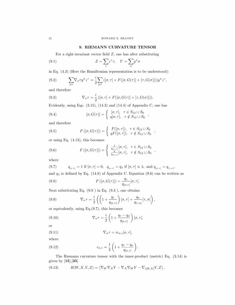
9. RIEMANN CURVATURE TENSOR

For a right-invariant vector field Z, one has after substituting

(9.1) Z =Xτ

zττ, Y =Xσ

yσσ

in Eq. (4.3) (Here the Hamiltonian representation is to be understood):

(9.2)Xστ

∇στyσzτ =

i

2

Xστ

([σ, τ ] + F ([σ,G(τ)] + [τ,G(σ)]))yσzτ ,

and therefore

(9.3) ∇στ =i

2([σ, τ ] + F ([σ,G(τ)] + [τ,G(σ)])).

Evidently, using Eqs. (3.15), (14.3) and (14.4) of Appendix C, one has

(9.4) [σ,G(τ)] =

½[σ, τ ], τ ∈ S12 ∪ S0q[σ, τ ], τ /∈ S12 ∪ S0 ,

and therefore

(9.5) F ([σ,G(τ)]) =

½F ([σ, τ ]), τ ∈ S12 ∪ S0qF ([σ, τ ]), τ /∈ S12 ∪ S0 ,

or using Eq. (4.13), this becomes

(9.6) F ([σ,G(τ)]) =

(1

q[σ,τ][σ, τ ], τ ∈ S12 ∪ S0

qq[σ,τ]

[σ, τ ], τ /∈ S12 ∪ S0 ,

where

(9.7) q[σ,τ]

= 1 if [σ, τ ] = 0, q[σ,τ ]

= qλ if [σ, τ ] ∝ λ, and q[σ,τ ]

= q[τ,σ]

,

and qλ is defined by Eq. (14.8) of Appendix C. Equation (9.6) can be written as

(9.8) F ([σ,G(τ)]) =qτ

q[σ,τ ][σ, τ ].

Next substituting Eq. (9.8 ) in Eq. (9.3 ), one obtains

(9.9) ∇στ =i

2

µµ1 +

qτq[σ,τ ]

¶[σ, τ ] +

qσq[τ,σ]

[τ, σ]

¶,

or equivalently, using Eq.(9.7), this becomes

(9.10) ∇στ =i

2

µ1 +

qτ − qσq[σ,τ ]

¶[σ, τ ],

or

(9.11) ∇στ = icσ,τ [σ, τ ],

where

(9.12) cσ,τ =1

2

µ1 +

qτ − qσq[σ,τ ]

¶.

The Riemann curvature tensor with the inner-product (metric) Eq. (3.14) isgiven by [15],[35]

(9.13) R(W,X, Y,Z) =∇W∇XY −∇X∇WY −∇i[W,X]Y,Z

®,


and after substituting the vector fields, expressed in terms of a basis of right-invariant frame fields ρ, σ, τ , and µ,

(9.14) W =Xσ

wρρ, X =Xσ

zσσ, Y =Xτ

yττ, Z =Xµ

zµµ,

Eq. (9.13) becomes

(9.15) Rρστµ =∇ρ∇στ −∇σ∇ρτ −∇i[ρ,σ]τ, µ

®.

Next, for three right-invariant vector fields X, Y , and Z, one has

(9.16) 0 = ∇Y hX,Zi = hX,∇Y Zi+ h∇YX,Zi ,or

(9.17) hX,∇Y Zi = − h∇YX,Zi ,and substituting Eqs. (9.14) in Eq. (9.17), one then has

(9.18) hσ,∇τµi = − h∇τσ, µi .Therefore

(9.19) h∇ρ∇στ, µi = − h∇στ,∇ρµi ,and

(9.20) h∇σ∇ρτ, µi = − h∇ρτ,∇σµi .Then substituting Eqs. (9.19) and (9.20) in Eq. (9.15), and interchanging the firstand second terms, one obtains

(9.21) Rρστµ = h∇ρτ,∇σµi− h∇στ,∇ρµi−∇i[ρ,σ]τ, µ

®.

Also clearly

(9.22) ∇iY Z = i∇Y Z,

so Eq. (9.21) can also be written as

(9.23) Rρστµ = h∇ρτ,∇σµi− h∇στ,∇ρµi− i∇[ρ,σ]τ, µ® .

Next substituting Eq. (9.11) in Eq. (9.23), one obtain the following useful form forthe Riemann curvature tensor [8], [43]-[45]:(9.24)Rρστµ = cρ,τ cσ,µ hi[ρ, τ ], i[σ,µ]i− cσ,τcρ,µ hi[σ, τ ], i[ρ, µ]i− c[ρ,σ],τ hi[i[ρ, σ], τ ], µi .The Riemannian curvature is important in determining the Jacobi field and theJacobi equation (See Section 11), and in investigations of the global characteristicsof geodesic paths in the group manifold [14].

10. SECTIONAL CURVATURE

The sectional curvature spanned by orthonormal right-invariant orthonormalvector fields X and Y is defined by [13]

(10.1) K(X,Y ) ≡ R(X,Y, Y,X)

|X|2|Y |2 − hX,Y i2 = R(X,Y, Y,X).

From Eqs. (9.14) and (9.21), it immediately follows that

(10.2) R(W,X, Y,Z) = h∇WY,∇XZi− h∇XY,∇WZi− ∇i[W,X]Y,Z®,

24 HOWARD E. BRANDT


(10.3) K(X,Y ) = h∇XY,∇YXi− h∇Y Y,∇XXi−∇i[X,Y ]Y,X

®.

Next it is useful to define

(10.4) B(X,Y ) = F (i[G(X), Y ]),

and using Eqs. (3.14) and Eq. (10.4), one obtains

(10.5) hB(X,Y ), Zi = hF (i[G(X), Y ]), Zi ,or equivalently, using Eq. (3.14), then

(10.6) hB(X,Y ), Zi = 1

2nTr(F (i[G(X), Y ])G(Z)).

Because the superoperator G is Hermitian, Eq. (10.6) can also be written as

(10.7) hB(X,Y ), Zi = 1

2nTr(GF (i[G(X), Y ])Z),

but according to Eq. (3.45) one has

(10.8) GF = I,

and therefore Eq. (10.7) becomes

(10.9) hB(X,Y ), Zi = 1

2nTr(i[G(X), Y ]Z).

Next expanding the commutator, Eq. (10.9) becomes

(10.10) hB(X,Y ), Zi = i

2nTr(G(X)Y Z − YG(X)Z),

and using the cyclic property of the trace, one obtains

(10.11) hB(X,Y ), Zi = i

2nTr(G(X)Y Z −G(X)ZY ),

or, equivalently,

(10.12) hB(X,Y ), Zi = i

2nTr(G(X)[Y,Z]).

But since the superoperator G is Hermitian, Eq. (10.12) can also be written as

(10.13) hB(X,Y ), Zi = i

2nTr(XG([Y,Z])),

or equivalently, using Eq. (3.14), this becomes

(10.14) hX, i[Y,Z]i = hB(X,Y ), Zi .But according to Eqs. (3.14), it follows that for vectors X and Y one has

(10.15) hX,Y i = 1

2nTr(XG(Y )),

and because the superoperator G is Hermitian, this can also be written as

(10.16) hX,Y i = 1

2nTr(G(X)Y ),

which by the cyclic invariance of the trace becomes

(10.17) hX,Y i = 1

2nTr(Y G(X)),


or equivalently using Eq. (3.14), it follows that

(10.18) hX,Y i = hY,Xi ,consistent with the Riemannian symmetric metric.

Next, for a right-invariant field Y , one has, using Eq. (4.3),

(10.19) ∇XY =1

2(i[X,Y ] + F (i[X,G(Y )]) + F (i[Y,G(X)])) ,

or

(10.20) ∇XY =1

2(i[X,Y ]− F (i[G(Y ),X])− F (i[G(X), Y ])) .


(10.21) ∇XY =1

2(i[X,Y ]−B(X,Y )−B(Y,X)) .

Next, according to Eq. (10.3), it follows that(10.22)

K(X,Y ) = R(X,Y, Y,X) = h∇XY,∇YXi− h∇Y Y,∇XXi− i∇[X,Y ]Y,X® .

According to Eq. (10.21), one has

(10.23) ∇[X,Y ]Y = 1

2(i[[X,Y ], Y ]−B([X,Y ], Y )−B(Y, [X,Y ])) .

Also using Eq. (10.21), one obtains(10.24)

h∇XY,∇YXi = 1

4(hi[X,Y ]−B(X,Y )−B(Y,X), i[Y,X]−B(Y,X)−B(X,Y )i) ,

or, equivalently,(10.25)

h∇XY,∇YXi = 1

4(hi[X,Y ]−B(X,Y )−B(Y,X),−i[X,Y ]−B(X,Y )−B(Y,X)i) ,

or

h∇XY,∇YXi = 1

4h−i[X,Y ], i[X,Y ]i

− 14hi[X,Y ], B(X,Y ) +B(Y,X)i+ 1

4hB(X,Y ) +B(Y,X), i[X,Y ]i

+1

4hB(X,Y ) +B(Y,X), B(X,Y ) +B(Y,X)i .(10.26)

Next using Eq. (10.18) in Eq. (10.26), then(10.27)

h∇XY,∇YXi = −14hi[X,Y ], i[X,Y ]i+1

4hB(X,Y ) +B(Y,X), B(X,Y ) +B(Y,X)i .

Also, one has

h∇Y Y,∇XXi = 1

4(h−i[Y, Y ], i[X,X]i− hi[Y, Y ], 2B(X,X)i+ h2B(Y, Y ), i[X,X]i

+ 4 hB(Y, Y ), B(X,X)i).(10.28)

But, according to Eq. (10.18 ), one has

(10.29) hB(Y,Y ), B(X,X)i = hB(X,X), B(Y, Y )i .Then simplifying, Eq. (10.28), one obtains

(10.30) h∇Y Y,∇XXi = hB(X,X), B(Y, Y )i .

26 HOWARD E. BRANDT

Next substituting Eqs. (10.27), (10.30), and (10.23) in Eq. (10.22), one has

K(X,Y ) = −14hi[X,Y ], i[X,Y ]i+ 1

4hB(X,Y ) +B(Y,X),B(X,Y ) +B(Y,X)i

− i

2hi[[X,Y ], Y ],Xi+ i

2hB([X,Y ], Y ),Xi+ i

2hB(Y, [X,Y ]),Xi

− hB(X,X), B(Y, Y )i .(10.31)

Expanding the third term of Eq. (10.31), one has, using Eq. (3.14),

− i

2hi[[X,Y ], Y ],Xi = 1

2

µ1

2n

¶Tr ([[X,Y ], Y ]G(X))

=1

2

µ1

2n

¶Tr( ([X,Y ]Y − Y [X,Y ])G(X)) ,(10.32)

and using the cyclic invariance of the trace, then

− i

2hi[[X,Y ], Y ],Xi = 1

2

µ1

2n

¶Tr([X,Y ]Y G(X)− [X,Y ])G(X)Y )

=1

2

µ1

2n

¶Tr(i[X,Y ]i[G(X), Y ]).(10.33)

Next using Eqs. (10.4), (3.14), and (3.45) in Eq. (10.33), one obtains

(10.34) − i

2hi[[X,Y ], Y ],Xi = 1

2hi[X,Y ], B(X,Y )i .

Next, in the fourth term of Eq. (10.31) one has, using Eq. (10.14),

(10.35) hB([X,Y ], Y ),Xi = h[X,Y ], i[Y,X]i = i hi[X,Y ], i[X,Y ]i .In the fifth term of Eq. (10.31), using Eq. (10.14), one has

(10.36) hB(Y, [X,Y ]),Xi = hY, i[[X,Y ],X]i ,or equivalently,

(10.37) hB(Y, [X,Y ]),Xi = hY, i[X, [Y,X]]i ,and using Eq. (10.14), this becomes

(10.38) hB(Y, [X,Y ]),Xi = − hB(Y,X), [X,Y ]i .Next using Eq. (10.18), Eq. (10.38) becomes

(10.39) hB(Y, [X,Y ]),Xi = − h[X,Y ], B(Y,X)i .Next, substituting Eqs. (10.34), (10.35), and (10.39) in Eq. (10.31), one has

K(X,Y ) = −14hi[X,Y ], i[X,Y ]i+ 1


+1

2hi[X,Y ], B(X,Y )i− 1

2hi[X,Y ], i[X,Y ]i− 1

2hi[X,Y ], B(Y,X)i

− hB(X,X), B(Y, Y )i ,(10.40)

and combining terms, this becomes [8], [43]-[45]

K(X,Y ) = −34hi[X,Y ], i[X,Y ]i+ 1


+1

2hi[X,Y ], B(X,Y )−B(Y,X)i− hB(X,X), B(Y, Y )i .(10.41)


11. JACOBI FIELD

Consider a one-parameter family of geodesics

(11.1) xj = xj(s, t),

in which the parameter s distinguishes a particular geodesic in the family, and t isthe usual curve parameter which can be taken to be time. The Riemannian geodesicequation in a coordinate representation is given by [13]

(11.2)∂2

∂t2xj(s) + Γjkl(s)

∂xk

∂t

∂xl

∂t= 0,

in which, according to Eq. (3.38) and the symmetry of the metric in its indices,

(11.3) Γjkl(s) =1

2gjm(s)(gkm,l(s) + glm,k(s)− gkl,m(s)),

for metric gij(s, x) ≡ gij(s).Let xj(0, t) be the base geodesic, and define the lifted Jacobi field along the

base geodesic by [8]

(11.4) Jj(t) =∂

∂sxj(s, t)|s=0,

describing how the base geodesic changes as the parameter s is varied. Using aTaylor series expansion, one has for small ∆s in the neighborhood of the basegeodesic,

(11.5) xj(∆s, t) = xj(0, t) +∆sJj(t) +O(∆s2).

Here xj(∆s, t) satisfies the geodesic equation with the metric gij(∆s). Operating

on the geodesic equation, Eq. (11.2) with ∂s ≡ ∂∂s and substituting Eqs. (11.4) and

(11.5), one obtains for ∆s→ 0,

0 =∂2

∂t2Lim∆s→0

∆sJj(t)

∆s+ Γjkl,m(s)|s=0 Lim∆s→0

∆sJm(t)

∆s

∂xk

∂t

∂xl

∂t+ ∂sΓ

jkl(s)|s=0

∂xk

∂t

∂xl

∂t

+ Γjkl(0)

½∂

∂t

µLim∆s→0

∆sJk(t)

∆s

¶∂xl

∂t+

∂xk

∂t

∂

∂tLim∆s→0

∆sJ l(t)

∆s

¾,

(11.6)

in which gij(0) ≡ gij is the base metric and Γjkl(0) ≡ Γjkl is the base connection.

Equation (11.6) then becomes

0 =∂2Jj(t)

∂t2+ Γjkl,m(s)|s=0J

m(t)∂xk

∂t

∂xl

∂t

+ ∂sΓjkl(s)|s=0

∂xk

∂t

∂xl

∂t+ Γjkl

µ∂Jk

∂t

∂xl

∂t+

∂xk

∂t

∂J l

∂t

¶.(11.7)

Taking account of dummy indices summed over, it is clearly true that

(11.8) −ΓjlqΓqik∂xi

∂t

∂xl

∂tJk + ΓjkpΓ

pmn

∂xk

∂t

∂xm

∂tJn = 0.

One also has

(11.9) −Γjik,l∂xi

∂t

∂xl

∂tJk + Γjkp,m

∂xm

∂t

∂xk

∂tJp = 0.

28 HOWARD E. BRANDT

Also, using the geodesic equation, Eq. (11.2), one has

(11.10) Γjkp∂2xk

∂t2Jp = −ΓjkpΓkiq

∂xi

∂t

∂xq

∂tJp,

or renaming dummy indices on the right hand side, it follows that

(11.11) Γjkp∂2xk

∂t2Jp + ΓjqkΓ

qil

∂xi

∂t

∂xl

∂tJk = 0.

Next adding Eqs. (11.7)-(11.9) and (11.11), one obtains

0 =∂2Jj(t)

∂t2+ Γjkl,mJ

m(t)∂xk

∂t

∂xl

∂t

+ ∂sΓjkl(s)|s=0

∂xk

∂t

∂xl

∂t+ Γjkl

µ∂Jk

∂t

∂xl

∂t+

∂xk

∂t

∂J l

∂t

¶− ΓjlqΓqlk

∂xi

∂t

∂xl

∂tJk + ΓjkpΓ

pmn

∂xk

∂t

∂xm

∂tJn

− Γjik,l∂xi

∂t

∂xl

∂tJk + Γjkp,m

∂xm

∂t

∂xk

∂tJp + Γjkp

∂2xk

∂t2Jp + ΓjqkΓ

qil

∂xi

∂t

∂xl

∂tJk,(11.12)

or equivalently,

∂2Jj(t)

∂t2= − Γjkl,m

∂xk

∂t

∂xl

∂tJm + ΓjlqΓ

qik

∂xi

∂t

∂xl

∂tJk

− ΓjkpΓpmn

∂xk

∂t

∂xm

∂tJn − ΓjqkΓqil

∂xi

∂t

∂xl

∂tJk + Γjik,l

∂xi

∂t

∂xl

∂tJk − Γjkp

∂2xk

∂t2Jp

− Γjklµ∂Jk

∂t

∂xl

∂t+

∂xk

∂t

∂J l

∂t

¶− ∂sΓ

jkl(s)|s=0

∂xk

∂t

∂xl

∂t− Γjkp,m

∂xm

∂t

∂xk

∂tJp.

(11.13)

Rearranging terms, then

∂2Jj(t)

∂t2= Γjik,l

∂xi

∂t

∂xl

∂tJk − Γjkl,m

∂xk

∂t

∂xl

∂tJm + ΓjlqΓ

qik

∂xi

∂t

∂xl

∂tJk

− ΓjkpΓpmn

∂xk

∂t

∂xm

∂tJn − Γjkp,m

∂xm

∂t

∂xk

∂tJp − Γjkp

∂2xk

∂t2Jp

− Γjkl∂xk

∂t

∂J l

∂t− Γjkl

∂xl

∂t

∂Jk

∂t

− ΓjqkΓqil∂xi

∂t

∂xl

∂tJk − ∂sΓ

jkl(s)|s=0

∂xk

∂t

∂xl

∂t.(11.14)

Noting that

(11.15) Γjqp = Γjpq,

and renaming dummy indices, Eq. (11.14) becomes

∂2Jj

∂t2=³Γjik,l − Γjil,k + ΓjlqΓqik − ΓjkpΓpli

´ ∂xi

∂t

∂xl

∂tJk

− Γjkp,m∂xm

∂t

∂xk

∂tJp − Γjkp

∂2xk

∂t2Jp − Γjkl

∂xk

∂t

∂J l

∂t

− Γjpk∂xk

∂t

µ∂Jp

∂t+ Γpmn

∂xm

∂tJn¶− ∂sΓ

jkl(s)|s=0

∂xk

∂t

∂xl

∂t.(11.16)


Next, using the expression for the covariant derivative, one has

D2Jj

Dt2=

∂

∂t

µDJj

Dt

¶+ Γjkp

∂xk

∂t

DJp

Dt

=∂

∂t

µ∂Jj

∂t+ Γjkp

∂xk

∂tJp¶+ Γjkp

∂xk

∂t

DJp

Dt,(11.17)

or

D2Jj

Dt2=

∂2Jj

∂t2+ Γjkp,m

∂xm

∂t

∂xk

∂tJp + Γjkp

∂2xk

∂t2Jp + Γjkp

∂xk

∂t

∂Jp

∂t

+ Γjkp∂xk

∂t

µ∂Jp

∂t+ Γpmn

∂xm

∂tJn¶.(11.18)

Also it is known that the Riemann curvature tensor is given by [35]

(11.19) Rjikl = Γ

jil,k − Γjik,l + ΓjkpΓpli − ΓjlqΓqik.

Substituting Eqs. (11.16) and (11.19) in Eq. (11.18), one obtains the so-calledlifted Jacobi equation [8],

(11.20)D2Jj

Dt2+Rj

ikl

∂xi

∂t

∂xl

∂tJk + ∂sΓ

jkl(s)|s=0

∂xk

∂t

∂xl

∂t= 0.

This equation is useful for investigations of the global behavior of geodesics andtheir extrapolation to nonvanishing values of the parameter s [8].

For gij independent of s, one has

(11.21) ∂sΓjkl(s)|s=0 = 0,

the last term of Eq. (11.20) is then vanishing, and one obtains the standard Jacobiequation for the Jacobi vector Jj [13],

(11.22)D2Jj

Dt2+Rj

ikl

∂xi

∂t

∂xl

∂tJk = 0.

Equation (11.22) is also known as the equation of geodesic deviation [20],[35],measuring the local convergence or divergence of neighboring geodesics, and it isuseful in the determination of geodesic conjugate points [13], [8].

Next consider the factor in the last term of the lifted Jacobi equation, Eq.(11.20),

(11.23) Ljkl ≡ ∂sΓjkl(s)|s=0.

Substituting Eq. (11.3) in Eq. (11.23), one has

(11.24) Ljkl ≡½∂s

·1

2gjm(s)(gkm,l(s) + glm,k(s)− gkl,m(s)

¸¾|s=0

,

or substituting Eq. (11.3),

(11.25) Ljkl ≡∂gjm(s)

∂s |s=0Γmkl +

1

2gjm(g0km,l + g0lm,k − g0kl,m),

in which

(11.26) g0km ≡ ∂sgkm(s)|s=0.

Next, the covariant derivative of g0km is given by [35]

(11.27) g0km;l = g0km,l − g0kiΓiml − g0miΓ

ikl.

30 HOWARD E. BRANDT

Then substituting Eq. (11.27) in Eq. (11.25) and using Eq. (11.15), one obtains

Ljkl ≡∂gjm(s)

∂s |s=0Γmkl +

1

2gjm(g0km;l + g0kiΓ

iml + g0miΓ

ikl

+ g0lm;k + g0liΓimk + g0miΓ

ikl

− g0kl;m − g0kiΓilm − g0liΓ

ikm),(11.28)

or

Ljkl ≡1

2gjm(g0km;l + g0lm;k − g0kl;m)

+∂gjm(s)

∂s |s=0Γmkl + gjmg0miΓ

ikl.(11.29)

Next, one notes that

(11.30) (gjmgmi)0 = (δji )

0 = 0,

and therefore

(11.31) gjm(0)

µ∂

∂sgmi(s)

¶|s=0

= −µ∂gjm(s)

∂s

¶|s=0

gmi(0).

Multiplying both side of Eq. (11.31) by Γikl, one obtains

(11.32) gjmg0miΓikl = −

µ∂gjm(s)

∂s

¶|s=0

Γmkl,

so that Eq. (11.29) reduces to

(11.33) Ljkl ≡1

2gjm(g0km;l + g0lm;k − g0kl;m).

Finally then combining Eqs. (11.20), (11.23) and (11.33), one obtains

(11.34)D2Jj

Dt2+Rj

ikl

∂xi

∂t

∂xl

∂tJk +

1

2gjm(g0km;l + g0lm;k − g0kl;m)

∂xk

∂t

∂xl

∂t= 0.

Next define the vector field,

(11.35) Cj ≡ 12gjm(g0km;l + g0lm;k − g0kl;m)

∂xk

∂t

∂xl

∂t, .

which is independent of the Jacobi field Jj . Equivalently, by symmetry, Eq. (11.35)can also be written as

(11.36) Cj ≡ 12gjm(2g0km;l − g0kl;m)

∂xk

∂t

∂xl

∂t.

Substituting Eq. (11.35) in Eq. (11.34), one obtains the second-order differentialequation,

(11.37)D2Jj

Dt2+Rj

ikl

∂xi

∂t

∂xl

∂tJk +Cj = 0,

the so-called ‘lifted Jacobi equation’ [8]. Nielsen and Dowling used the lifted Jacobiequation, Eq. (11.37), to deform geodesics from the value q = 1 for the penaltyparameter to much larger values, and this enabled them to define a so-called geo-desic derivative and to deform a geodesic as the penalty parameter is varied withoutchanging the fixed values U = 1 and U = Uf of the initial and final unitary trans-formation corresponding to the quantum computation [8].


12. APPENDIX A: PAULI MATRICES

The Pauli matrices are defined by [1](12.1)

σ0 ≡ I ≡·1 00 1

¸, σ1 ≡ X ≡

·0 11 0

¸, σ2 ≡ Y ≡

·0 −ii 0

¸, σ3 ≡ Z ≡

·1 00 −1

¸,

They are Hermitian,

(12.2) σi = σ†i , i = 0, 1, 2, 3,

and, except for σ0, they are traceless,

(12.3) Trσi = 0, i 6= 0.Their products are given by

(12.4) σ2i = I,

and, using the Einstein sum convention for repeated indices (both lower in thiscase),

(12.5) σiσj = iεijkσk, i, j, k 6= 0,expressed in terms of the totally antisymmetric Levi-Civita symbol with ε123 = 1.Quantum gates can be expressed in terms of tensor products of Pauli matrices. Forexample the CNOT gate [1] can be expressed as follows:

(12.6) CNOT =

1 0 0 00 1 0 00 0 0 10 0 1 0

= 1

2(I ⊗ I + I ⊗ σ1 + σ3 ⊗ I − σ3 ⊗ σ1).

13. APPENDIX B: SUPEROPERATOR ADJOINTS

The purpose of this Appendix is to derive Eqs. (3.12) and (3.13) for the adjoint

superoperators E†X and D†X (at least to first order). For vectors X,Y,Z, consider

the trace inner product defined by

(13.1) (Y, adXZ) ≡ Tr¡Y †adXZ

¢,

or using Eq. (3.7), this becomes

(13.2) (Y, adXZ) ≡ Tr¡Y †[X,Z]

¢,

or expanding the commutator, then

(13.3) (Y, adXZ) ≡ Tr¡Y †XZ − Y †ZX

¢.

Next using the cyclic property of the trace, Eq. (13.3) becomes

(13.4) (Y, adXZ) ≡ Tr¡Y †XZ −XY †Z

¢,

or equivalently, again using the trace inner product,

(13.5) (Y, adXZ) ≡ −Tr¡[X,Y †]Z

¢= − ¡[X,Y †]†, Z

¢,

or

(13.6) (Y, adXZ) ≡ −¡[Y,X†], Z

¢=¡[X†, Y ], Z

¢.

But by definition of the adjoint, one has

(13.7) (Y, adXZ) ≡³ad†XY,Z

´,

32 HOWARD E. BRANDT

and comparing Eqs. (13.6) and (13.7), one obtains

(13.8) ad†XY = [X†, Y ].

Next, if X is Hermitian, then X = X†, and Eq. (13.8) becomes

(13.9) ad†XY = [X,Y ] = adXY,

and it follows that adX is Hermitian,

(13.10) ad†X = adX .

Also, Eq. (3.7) implies

(13.11) adXY = [X,Y ] = −[−X,Y ] = −ad−XY,and therefore

(13.12) adX = −ad−X .Next, Eqs. (3.10) and (13.10) imply

(13.13) E†X = I +

i

2adX +O(X2).

Also according to Eqs. (3.10) and (13.12), one has

(13.14) E−X = I +i

2adX +O(X2).

Comparing Eqs. (13.13) and (13.14), one has (at least to first order),

(13.15) E†X = E−X .

Also, according to Eqs. (3.9) and (3.10),

(13.16) DX = E−1X = I +i

2adX +O(X2).

Then

(13.17) D†X = I − i

2ad†X +O(x2),

and substituting Eq. (13.10) and using Eq. (13.12), then

(13.18) D†X = I +

i

2ad−X +O(x2).

Also, Eq. (13.16) implies that

(13.19) D−X = I +i

2ad−X +O(x2).

Comparing Eqs. (13.18) and (13.19), then (at least to first order) one has

(13.20) D†X = D−X .


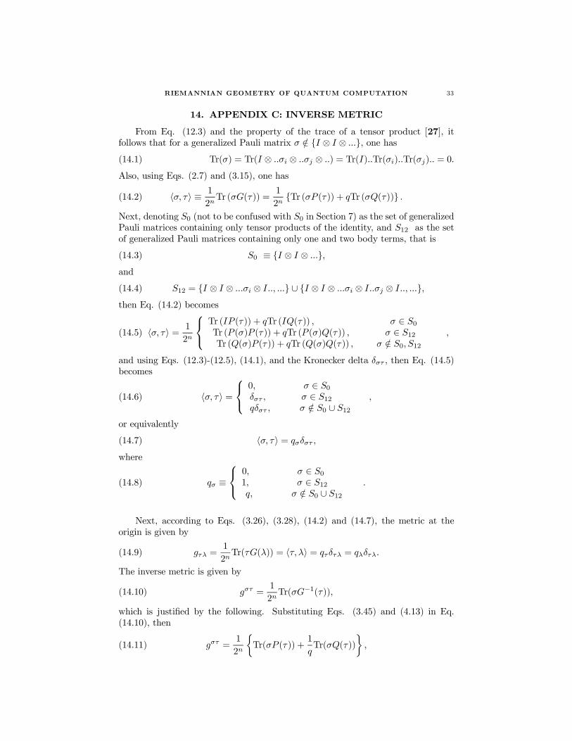
14. APPENDIX C: INVERSE METRIC

From Eq. (12.3) and the property of the trace of a tensor product [27], itfollows that for a generalized Pauli matrix σ /∈ {I ⊗ I ⊗ ...}, one has(14.1) Tr(σ) = Tr(I ⊗ ..σi ⊗ ..σj ⊗ ..) = Tr(I)..Tr(σi)..Tr(σj).. = 0.

Also, using Eqs. (2.7) and (3.15), one has

(14.2) hσ, τi ≡ 1

2nTr (σG(τ)) =

1

2n{Tr (σP (τ)) + qTr (σQ(τ))} .

Next, denoting S0 (not to be confused with S0 in Section 7) as the set of generalizedPauli matrices containing only tensor products of the identity, and S12 as the setof generalized Pauli matrices containing only one and two body terms, that is

(14.3) S0 ≡ {I ⊗ I ⊗ ...},and

(14.4) S12 = {I ⊗ I ⊗ ...σi ⊗ I.., ...} ∪ {I ⊗ I ⊗ ...σi ⊗ I..σj ⊗ I.., ...},then Eq. (14.2) becomes

(14.5) hσ, τi = 1

2n

Tr (IP (τ)) + qTr (IQ(τ)) , σ ∈ S0Tr (P (σ)P (τ)) + qTr (P (σ)Q(τ)) , σ ∈ S12Tr (Q(σ)P (τ)) + qTr (Q(σ)Q(τ)) , σ /∈ S0, S12

,

and using Eqs. (12.3)-(12.5), (14.1), and the Kronecker delta δστ , then Eq. (14.5)becomes

(14.6) hσ, τi = 0, σ ∈ S0

δστ , σ ∈ S12qδστ , σ /∈ S0 ∪ S12

,

or equivalently

(14.7) hσ, τi = qσδστ ,

where

(14.8) qσ ≡ 0, σ ∈ S01, σ ∈ S12q, σ /∈ S0 ∪ S12

.

Next, according to Eqs. (3.26), (3.28), (14.2) and (14.7), the metric at theorigin is given by

(14.9) gτλ =1

2nTr(τG(λ)) = hτ, λi = qτδτλ = qλδτλ.

The inverse metric is given by

(14.10) gστ =1

2nTr(σG−1(τ)),

which is justified by the following. Substituting Eqs. (3.45) and (4.13) in Eq.(14.10), then

(14.11) gστ =1

2n

½Tr(σP (τ)) +

1

qTr(σQ(τ))

¾,

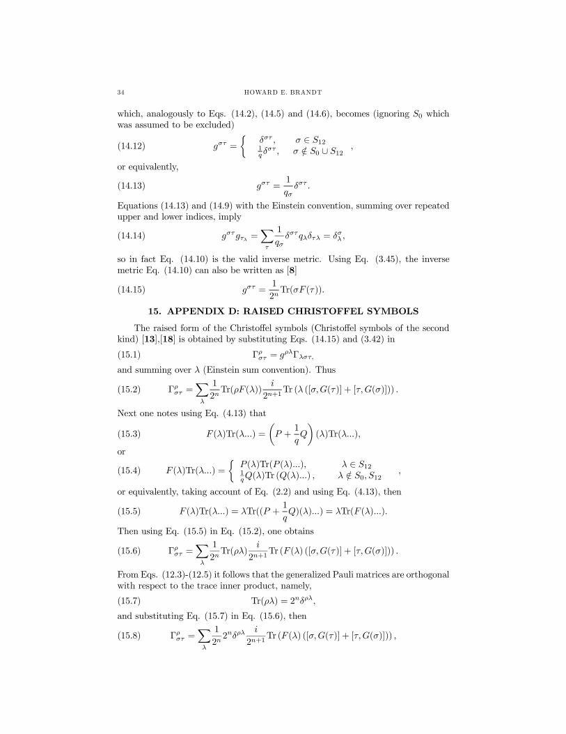
34 HOWARD E. BRANDT

which, analogously to Eqs. (14.2), (14.5) and (14.6), becomes (ignoring S0 whichwas assumed to be excluded)

(14.12) gστ =

½δστ , σ ∈ S121q δ

στ , σ /∈ S0 ∪ S12 ,

or equivalently,

(14.13) gστ =1

qσδστ .

Equations (14.13) and (14.9) with the Einstein convention, summing over repeatedupper and lower indices, imply

(14.14) gστgτλ =Xτ

1

qσδστqλδτλ = δσλ ,

so in fact Eq. (14.10) is the valid inverse metric. Using Eq. (3.45), the inversemetric Eq. (14.10) can also be written as [8]

(14.15) gστ =1

2nTr(σF (τ)).

15. APPENDIX D: RAISED CHRISTOFFEL SYMBOLS

The raised form of the Christoffel symbols (Christoffel symbols of the secondkind) [13],[18] is obtained by substituting Eqs. (14.15) and (3.42) in

(15.1) Γρστ = gρλΓλστ,

and summing over λ (Einstein sum convention). Thus

(15.2) Γρστ =Xλ

1

2nTr(ρF (λ))

i

2n+1Tr (λ ([σ,G(τ)] + [τ,G(σ)])) .

Next one notes using Eq. (4.13) that

(15.3) F (λ)Tr(λ...) =

µP +

1

qQ

¶(λ)Tr(λ...),

or

(15.4) F (λ)Tr(λ...) =

½P (λ)Tr(P (λ)...), λ ∈ S121qQ(λ)Tr (Q(λ)...) , λ /∈ S0, S12

,

or equivalently, taking account of Eq. (2.2) and using Eq. (4.13), then

(15.5) F (λ)Tr(λ...) = λTr((P +1

qQ)(λ)...) = λTr(F (λ)...).

Then using Eq. (15.5) in Eq. (15.2), one obtains


1

2nTr(ρλ)

i

2n+1Tr (F (λ) ([σ,G(τ)] + [τ,G(σ)])) .

From Eqs. (12.3)-(12.5) it follows that the generalized Pauli matrices are orthogonalwith respect to the trace inner product, namely,

(15.7) Tr(ρλ) = 2nδρλ,

and substituting Eq. (15.7) in Eq. (15.6), then


1

2n2nδρλ

i

2n+1Tr (F (λ) ([σ,G(τ)] + [τ,G(σ)])) ,


or finally,

(15.9) Γρστ =i

2n+1Tr (F (ρ) ([σ,G(τ)] + [τ,G(σ)])) .

16. APPENDIX E: AN IDENTITY

In this Appendix, the identity given by Eq. (3.49) is derived. It follows fromEq. (12.4) and (12.5) that for some coefficients aτλσ and bτλ one has

(16.1) [τ,G(λ)] =Xσ

aτλσσ + bτλI.

Then multiplying both sides of Eq. (16.1) by κ and taking the trace, one obtains

(16.2) Tr (κ[τ,G(λ)]) =Xσ

aτλσTr(κσ) + bτλTr(κ).

Next substituting Eqs. (12.3) and (15.7) in Eq. (16.2), the latter becomes

(16.3) Tr (κ[τ,G(λ)]) =Xσ

aτλσ2nδκσ = 2

naτλκ,

and therefore

(16.4) aτλσ =1

2nTr (σ[τ,G(λ)]) .

Next operating on both sides of Eq. (16.1) with F , and using Eq. (4.13), one has

(16.5) F ([τ,G(λ)]) =Xσ

aτλσF (σ),


(16.6) F ([τ,G(λ)]) =Xσ

F (σ)1

2nTr (σ[τ,G(λ)]) ,

or

(16.7) 2nF ([τ,G(λ)]) =Xσ

F (σ)Tr (σ[τ,G(λ)]) .


(16.8) 2nF ([τ,G(λ)]) =Xσ

σTr (F (σ)[τ,G(λ)]) ,

or equivalently,

(16.9)Xσ

σTr (F (σ)[τ,G(λ)]) = 2nF ([τ,G(λ)]) .

which is Eq. (3.49).

36 HOWARD E. BRANDT

17. APPENDIX F: CHECKS OF THREE-QUBIT SOLUTIONS

In this Appendix, checks are given of the solution, Eq. (7.28) to Eq. (7.16),

(17.1) Q(t) = eit(q−1−s−1)S0Q0e−it(q

−1−s−1)S0 ,

and the solution, Eq. (7.57) to Eq. (7.15),

(17.2) T (t) = eit(q−1−s−1)S0eit(1−q

−1)(S0+Q0)T0e−it(1−q−1)(S0+Q0)e−it(q

−1−s−1)S0 .

A check that Eq. (17.1) does indeed satisfy Eq. (7.16) proceeds by first calcu-lating

dQ

dt= i(q−1 − s−1)S0Q(t)− i(q−1 − s−1)Q(t)S0(17.3)

= i(q−1 − s−1)[S0, Q(t)],

which agrees with Eqs. (7.16) and (7.17).Proceeding to check that Eq. (17.2) satisfies Eq. (7.15), it follows from Eq.

(17.2) that

dT

dt= i(q−1 − s−1)S0T (t)− i(q−1 − s−1)T (t)S0 + eit(q

−1−s−1)S0

× d

dt

³eit(1−q

−1)(S0+Q0)T0e−it(1−q−1)(S0+Q0)

´e−it(q

−1−s−1)S0

= i(q−1 − s−1)[S0, T (t)] + eit(q−1−s−1)S0{i(1− q−1)

× [(S0 +Q0), eit(1−q−1)(S0+Q0)T0e

−it(1−q−1)(S0+Q0)]}× e−it(q

−1−s−1)S0 .(17.4)

The following commutation relation is true:

(17.5) [A,BC] = ABC−BCA = BAC−BCA+ABC−BAC = B[A,C]+[A,B]C,

and using Eq. (17.5) twice, and noting that (S0 +Q0) commutes with itself, Eq.(17.4) becomes

dT

dt= i(q−1 − s−1)[S0, T (t)] + eit(q

−1−s−1)S0i(1− q−1)

×neit(1−q

−1)(S0+Q0)[(S0 +Q0), T0e−it(1−q−1)(S0+Q0)]

+ [(S0 +Q0), eit(1−q−1)(S0+Q0)]T0e

−it(1−q−1)(S0+Q0)o

× e−it(q−1−s−1)S0 ,(17.6)

or

dT

dt= i(q−1 − s−1)[S0, T (t)] + eit(q

−1−s−1)S0i(1− q−1)

×neit(1−q

−1)(S0+Q0)T0[(S0 +Q0), e−it(1−q−1)(S0+Q0)]

+ eit(1−q−1)(S0+Q0)[(S0 +Q0), T0]e

−it(1−q−1)(S0+Q0)o

× e−it(q−1−s−1)S0 .(17.7)


Equivalently then,

dT

dt= i(q−1 − s−1)[S0, T (t)]

+ eit(q−1−s−1)S0i(1− q−1)eit(1−q

−1)(S0+Q0)[(S0 +Q0), T0]

× e−it(1−q−1)(S0+Q0)e−it(q

−1−s−1)S0 ,(17.8)

or

dT

dt= i(q−1 − s−1)[S0, T (t)] + i(1− q−1)eit(q

−1−s−1)S0

× (S0 +Q0)eit(1−q−1)(S0+Q0)T0e

−it(1−q−1)(S0+Q0)

× e−it(q−1−s−1)S0

− i(1− q−1)eit(q−1−s−1)S0eit(1−q

−1)(S0+Q0)T0

× e−it(1−q−1)(S0+Q0)

× (S0 +Q0)e−it(q−1−s−1)S0 .(17.9)

This becomes

dT

dt= i(q−1 − s−1)[S0, T (t)] + i(1− q−1)eit(q

−1−s−1)S0

×Q0eit(1−q−1)(S0+Q0)T0e

−it(1−q−1)(S0+Q0)e−it(q−1−s−1)S0

− i(1− q−1)eit(q−1−s−1)S0eit(1−q

−1)(S0+Q0)T0

× e−it(1−q−1)(S0+Q0)Q0e

−it(q−1−s−1)S0

+ i(1− q−1)eit(q−1−s−1)S0

× [S0, eit(1−q−1)(S0+Q0)T0e−it(1−q−1)(S0+Q0)]e−it(q

−1−s−1)S0 .(17.10)

38 HOWARD E. BRANDT

Next, the right side of Eq. (7.15), using Eqs. (7.17), (7.28), and (7.57), becomes

i[((1− s−1)S + (1− q−1)Q), T ]

= i(1− s−1)[S, T ] + i(1− q−1)[Q,T ]

= i[S0, T ]− is−1[S0, T ] + i(1− q−1)[Q,T ]

= i[S0, T ]− is−1[S0, T ] + i(1− q−1)

× [eit(q−1−s−1)S0Q0e−it(q−1−s−1)S0 , eit(q−1−s−1)S0eit(1−q−1)(S0+Q0)

× T0e−it(1−q−1)(S0+Q0)e−it(q

−1−s−1)S0 ]

= i(1− q−1)[S0, T ] + i(q−1 − s−1)[S0, T ]

+ i(1− q−1)eit(q−1−s−1)S0Q0eit(1−q

−1)(S0+Q0)T0

× e−it(1−q−1)(S0+Q0)e−it(q

−1−s−1)S0

− i(1− q−1)eit(q−1−s−1)S0eit(1−q

−1)(S0+Q0)T0

× e−it(1−q−1)(S0+Q0)Q0e

−it(q−1−s−1)S0

= i(q−1 − s−1)[S0, T ]

+ i(1− q−1)[S0, eit(q−1−s−1)S0eit(1−q

−1)(S0+Q0)T0

× e−it(1−q−1)(S0+Q0)e−it(q

−1−s−1)S0 ]

+ i(1− q−1)eit(q−1−s−1)S0Q0eit(1−q

−1)(S0+Q0)T0

× e−it(1−q−1)(S0+Q0)e−it(q

−1−s−1)S0

− i(1− q−1)eit(q−1−s−1)S0eit(1−q

−1)(S0+Q0)T0

× e−it(1−q−1)(S0+Q0)Q0e

−it(q−1−s−1)S0 .(17.11)

Equivalently then,


i[((1− s−1)S + (1− q−1)Q), T ]

= i(q−1 − s−1)[S0, T ]

+ i(1− q−1)eit(q−1−s−1)S0Q0eit(1−q

−1)(S0+Q0)T0

× e−it(1−q−1)(S0+Q0)e−it(q

−1−s−1)S0

− i(1− q−1)eit(q−1−s−1)S0eit(1−q

−1)(S0+Q0)T0

× e−it(1−q−1)(S0+Q0)Q0e

−it(q−1−s−1)S0

+ i(1− q−1)eit(q−1−s−1)S0eit(1−q

−1)(S0+Q0)T0

× e−it(1−q−1)(S0+Q0)[S0, e

−it(q−1−s−1)S0 ]

+ i(1− q−1)eit(q−1−s−1)S0 [S0, eit(1−q

−1)(S0+Q0)T0

× e−it(1−q−1)(S0+Q0)]e−it(q

−1−s−1)S0

= i(q−1 − s−1)[S0, T ]

+ i(1− q−1)eit(q−1−s−1)S0Q0eit(1−q

−1)(S0+Q0)T0

× e−it(1−q−1)(S0+Q0)e−it(q

−1−s−1)S0

− i(1− q−1)eit(q−1−s−1)S0eit(1−q

−1)(S0+Q0)T0

× e−it(1−q−1)(S0+Q0)Q0e

−it(q−1−s−1)S0

+ i(1− q−1)eit(q−1−s−1)S0 [S0, eit(1−q

−1)(S0+Q0)T0

× e−it(1−q−1)(S0+Q0)]e−it(q

−1−s−1)S0 .(17.12)

Comparing Eqs. (17.12), (17.10), and (7.15), one concludes that the left and rightsides of Eq. (7.15) agree.

References

[1] M. A. Nielsen and I. L. Chuang, Quantum Information and Computation (Cambridge Uni-versity Press, 2000).

[2] R. Montgomery, A Tour of Sub-Riemannian Geometries, Their Geodesics and Applications,Vol. 91 of Mathematical Surveys and Monographs (American Mathematical Society, Provi-dence, Rhode Island, 2002).

[3] N. Khaneja, S. J. Glaser, and R. Brockett, "Sub-Riemannian Geometry and Time OptimalControl of Three Spin Systems: Quantum Gates and Coherence Transfer," Phys. Rev. A 65,032301(1-11) (2002).

[4] C. G. Moseley, "Geometric control of quantum spin systems," in Quantum Information andComputation II, edited by E. Donkor, A. R. Pirich, and H. E. Brandt, Proc. SPIE Vol. 5436,pp. 319-323, SPIE, Bellingham, WA (2004).

[5] M. A. Nielsen, "A Geometric Approach to Quantum Circuit Lower Bounds," Quantum In-formation and Computation 6, 213-262 (2006).

[6] M. A. Nielsen, M. R. Dowling, M. Gu, and A. C. Doherty, "Optimal Control, Geometry, andQuantum Computing," Phys. Rev. A 73, 062323(1-7) (2006).

[7] M. A. Nielsen, M. R. Dowling, M. Gu, and A. C. Doherty, "Quantum Computation asGeometry," Science 311, 1133-1135 (2006).

[8] M. R. Dowling and M. A. Nielsen, "The Geometry of Quantum Computation," QuantumInformation and Computation 8, 0861-0899 (2008).

40 HOWARD E. BRANDT

[9] J. N. Clelland and C. G. Moseley, "Sub-Finsler Geometry in Dimension Three," DifferentialGeometry and its Applications 24, 628-651 (2006).

[10] Bo-Yu Hou and Bo-Yuan Hou, Differential Geometry for Physicists (World Scientific, Sin-gapore, 1997).

[11] A. A. Sagle and R. E. Walde, Introduction to Lie Groups and Lie Algebras, Academic Press,New York (1973).

[12] L. Conlon, Differentiable Manifolds, 2nd Edition, Birkhäuser, Boston (2001).[13] J. M. Lee, Riemannian Manifolds: An Introduction to Curvature, Springer, New York (1997).[14] M. Berger, A Panoramic View of Riemannian Geometry, Springer-Verlag, Berlin (2003).[15] B. C. Hall, Lie Groups, Lie Algebras, and Representations, Springer, New York (2004).[16] J. Farout, Analysis on Lie Groups, Cambridge University Press, Cambridge, UK (2008).[17] M. M. Postnikov, Geometry VI: Riemannian Geometry, Encyclopedia of Mathematical Sci-

ences, vol. 91, Springer-Verlag, Berlin (2001).[18] P. Petersen, Riemannian Geometry, 2nd Edition, Springer, New York (2006).[19] J. Jost, Riemannian Geometry and Geometric Analysis, 5th Edition, Springer-Verlag, Berlin

(2008).[20] R. Wasserman, Tensors and Manifolds, 2nd Edition, Oxford University Press, Oxford, UK

(2004).[21] M. A. Naimark and A. I. Stern, Theory of Group Representations, Springer-Verlag, New

York (1982).[22] Mark R. Sepanski, Compact Lie Groups, Springer (2007).[23] Walter Pfeifer, The Lie Algebras su(N), Birkhäuser, Basel, (2003).[24] John Stillwell, Naive Lie Theory, Springer, NY (2008).[25] J. F. Cornwell, Group Theory in Physics: An Introduction, Academic Press, San Diego, CA

(1997).[26] J. F. Cornwell, Group Theory in Physics, Vol. 2, Academic Press, London (1984).[27] W. Steeb and Y. Hardy, Problems and Solutions in Quantum Computing and Quantum

Information, 2nd Edition, World Scientific, New Jersey (2006).[28] S. Weigert, "Baker-Campbell-Hausdorff Relation for Special Unitary Groups SU(N)," J. Phys.

A: Math. Gen. 30, 8739-8749 (1997).[29] C. Reutenauer, Free Lie Algebras, Clarendon Press, Oxford (1993).[30] E. Dynkin, "Calculation of the coefficients in the Campbell-Hausdorff formula," Dokl. Akad.

Nauk 57, 323-326 (1947).[31] H. F. Baker, "Alternants and continuous groups," Proc. London Math. Soc. (2) 3, 24-47

(1905).[32] J. E. Campbell, "On a law of combination of operators bearing on the theory of continuous

transformation groups," Proc. London Math. Soc. (1) 28, 381-390 (1897).[33] J. E. Campbell, "On a law of combination of operators," Proc. London Math. Soc. (1) 29,

14-32, (1898).[34] F. Hausdorff, "Die symbolische Exponentialformel in der Gruppentheorie," Leipziger Berichte

58, 19-48 (1906).[35] C. W. Misner, K. S. Thorne, and J. A. Wheeler, Gravitation, pp. 223, 224, 310, W. H.

Freeman and Company, New York (1973).[36] P. D. Lax, "Integrals of Nonlinear Equations of Evolution and Solitary Waves," Communi-

cations on Pure and Applied Math. 21, 467-490 (1968).[37] R. Abraham and J. E. Marsden, Foundations of Mechanics, 2nd Edition, AMS Chelsea

Publishing, American Mathematical Society, Providence, Rhode Island (2008).[38] D. Zwillinger, Handbook of Differential Equations, Third Edition, Academic Press, San Diego,

CA (1998).[39] R. S. Kaushal and D. Parashar, Advanced Methods of Mathematical Physics, CRC Press,

Boca Raton, FL (2000).[40] T. Miwa, M. Jimbo, and E. Date, Solitons, Cambridge University Press, Cambridge, UK

(2000).[41] L. Debnath, Nonlinear Partial Differential Equations, Birkhäuser, Boston, MA (1997).[42] E. Zeidler, Nonlinear Functional Analysis and its Applications IV: Applications to Mathe-

matical Physics, Springer-Verlag, New York, NY (1997).[43] J. Milnor, "Curvatures of Left Invariant Metrics on Lie Groups," Advances in Mathematics

21, 293-329 (1976).


[44] V. I. Arnold, Mathematical Methods of Classical Mechanics, 2nd Edition, Springer-Verlag,New York (1989).

[45] V. I. Arnold and B. A. Khesin, Topological Methods in Hydrodynamics, Springer, New York(1999).

U.S. Army Research Laboratory, Adelphi, MDE-mail address : [email protected]

Riemannian Geometry of Quantum Computationlomonaco/ams2009-talks/Brandt-Paper... · Proceedings of...

Documents

Transcript of Riemannian Geometry of Quantum Computationlomonaco/ams2009-talks/Brandt-Paper... · Proceedings of...