Riemannian Geometry - University of Manchester

Riemannian Geometry

it is a draft of Lecture Notes of H.M. Khudaverdian.Manchester, 20-th May 2011

Contents

1 Riemannian manifolds 41.1 Manifolds. Tensors. (Recalling) . . . . . . . . . . . . . . . . . 41.2 Riemannian manifold—manifold equipped with Riemannian

metric . . . . . . . . . . . . . . . . . . . . . . . . . . . . . . . 71.2.1 ∗ Pseudoriemannian manifold . . . . . . . . . . . . . . 11

1.3 Scalar product. Length of tangent vectors and angle betweenvectors. Length of the curve . . . . . . . . . . . . . . . . . . . 111.3.1 Length of the curve . . . . . . . . . . . . . . . . . . . . 12

1.4 Riemannian structure on the surfaces embedded in Euclideanspace . . . . . . . . . . . . . . . . . . . . . . . . . . . . . . . . 151.4.1 Internal and external coordinates of tangent vector . . 151.4.2 Explicit formulae for induced Riemannian metric (First

Quadratic form) . . . . . . . . . . . . . . . . . . . . . . 171.4.3 Induced Riemannian metrics. Examples. . . . . . . . . 201.4.4 ∗Induced metric on two-sheeted hyperboloid embedded

in pseudo-Euclidean space. . . . . . . . . . . . . . . . . 271.5 Isometries of Riemanian manifolds. . . . . . . . . . . . . . . . 28

1.5.1 Examples of local isometries . . . . . . . . . . . . . . . 291.6 Volume element in Riemannian manifold . . . . . . . . . . . . 31

1.6.1 Volume of parallelepiped . . . . . . . . . . . . . . . . . 311.6.2 Invariance of volume element under changing of coor-

dinates . . . . . . . . . . . . . . . . . . . . . . . . . . . 331.6.3 Examples of calculating volume element . . . . . . . . 34

1

2 Covariant differentiaion. Connection. Levi Civita Connec-tion on Riemannian manifold 362.1 Differentiation of vector field along the vector field.—Affine

connection . . . . . . . . . . . . . . . . . . . . . . . . . . . . . 362.1.1 Definition of connection. Christoffel symbols of con-

nection . . . . . . . . . . . . . . . . . . . . . . . . . . . 372.1.2 Transformation of Christoffel symbols for an arbitrary

connection . . . . . . . . . . . . . . . . . . . . . . . . . 392.1.3 Canonical flat affine connection . . . . . . . . . . . . . 402.1.4 ∗ Global aspects of existence of connection . . . . . . . 43

2.2 Connection induced on the surfaces . . . . . . . . . . . . . . . 442.2.1 Calculation of induced connection on surfaces in E3. . . 45

2.3 Levi-Civita connection . . . . . . . . . . . . . . . . . . . . . . 472.3.1 Symmetric connection . . . . . . . . . . . . . . . . . . 472.3.2 Levi-Civita connection. Theorem and Explicit formulae 472.3.3 Levi-Civita connection on 2-dimensional Riemannian

manifold with metric G = adu2 + bdv2. . . . . . . . . . 492.3.4 Example of the sphere again . . . . . . . . . . . . . . . 49

2.4 Levi-Civita connection = induced connection on surfaces in E3 50

3 Parallel transport and geodesics 523.1 Parallel transport . . . . . . . . . . . . . . . . . . . . . . . . . 52

3.1.1 Definition . . . . . . . . . . . . . . . . . . . . . . . . . 523.1.2 ∗Parallel transport is a linear map . . . . . . . . . . . 533.1.3 Parallel transport with respect to Levi-Civita connection 54

3.2 Geodesics . . . . . . . . . . . . . . . . . . . . . . . . . . . . . 543.2.1 Definition. Geodesic on Riemannian manifold. . . . . . 543.2.2 Un-parameterised geodesic . . . . . . . . . . . . . . . . 553.2.3 Geodesics on surfaces in E3 . . . . . . . . . . . . . . . 56

3.3 Geodesics and Lagrangians of ”free” particle on Riemannianmanifold. . . . . . . . . . . . . . . . . . . . . . . . . . . . . . . 583.3.1 Lagrangian and Euler-Lagrange equations . . . . . . . 583.3.2 Lagrangian of ”free” particle . . . . . . . . . . . . . . . 583.3.3 Equations of geodesics and Euler-Lagrange equations . 593.3.4 Examples of calculations of Christoffel symbols and

geodesics using Lagrangians. . . . . . . . . . . . . . . . 603.3.5 Variational principe and Euler-Lagrange equations . . 62

3.4 Geodesics and shortest distance. . . . . . . . . . . . . . . . . . 63

2

3.4.1 Again geodesics for sphere and Lobachevsky plane . . . 65

4 Surfaces in E3 674.1 Formulation of the main result. Theorem of parallel transport

over closed curve and Theorema Egregium . . . . . . . . . . . 674.1.1 GaußTheorema Egregium . . . . . . . . . . . . . . . . . 69

4.2 Derivation formulae . . . . . . . . . . . . . . . . . . . . . . . 704.2.1 ∗Gauss condition (structure equations) . . . . . . . . . 72

4.3 Geometrical meaning of derivation formulae. Weingarten op-erator and second quadratic form in terms of derivation for-mulae. . . . . . . . . . . . . . . . . . . . . . . . . . . . . . . 734.3.1 Gaussian and mean curvature in terms of derivation

formulae . . . . . . . . . . . . . . . . . . . . . . . . . . 754.4 Examples of calculations of derivation formulae and curvatures

for cylinder, cone and sphere . . . . . . . . . . . . . . . . . . 764.5 ∗Proof of the Theorem of parallel transport along closed curve. 80

5 Curvtature tensor 845.1 Definition . . . . . . . . . . . . . . . . . . . . . . . . . . . . . 84

5.1.1 Properties of curvature tensor . . . . . . . . . . . . . . 855.2 Riemann curvature tensor of Riemannian manifolds. . . . . . . 865.3 †Curvature of surfaces in E3.. Theorema Egregium again . . . 875.4 Relation between Gaussian curvature and Riemann curvature

tensor. Straightforward proof of Theorema Egregium . . . . . 885.4.1 ∗Proof of the Proposition (5.25) . . . . . . . . . . . . . 90

5.5 Gauss Bonnet Theorem . . . . . . . . . . . . . . . . . . . . . . 94

6 Appendices 976.1 ∗Integrals of motions and geodesics. . . . . . . . . . . . . . . . 97

6.1.1 ∗Integral of motion for arbitrary Lagrangian L(x, x) . . 976.1.2 ∗Basic examples of Integrals of motion: Generalised

momentum and Energy . . . . . . . . . . . . . . . . . . 976.1.3 ∗Integrals of motion for geodesics . . . . . . . . . . . . 986.1.4 ∗Using integral of motions to calculate geodesics . . . . 100

6.2 Induced metric on surfaces. . . . . . . . . . . . . . . . . . . . 1016.2.1 Recalling Weingarten operator . . . . . . . . . . . . . . 1016.2.2 Second quadratic form . . . . . . . . . . . . . . . . . . 1026.2.3 Gaussian and mean curvatures . . . . . . . . . . . . . . 103

3

6.2.4 Examples of calculation of Weingarten operator, Sec-ond quadratic forms, curvatures for cylinder, cone andsphere. . . . . . . . . . . . . . . . . . . . . . . . . . . . 103

1 Riemannian manifolds

1.1 Manifolds. Tensors. (Recalling)

I recall briefly basics of manifolds and tensor fields on manifolds.An n-dimensional manifold is a space such that in a vicinity of any point

one can consider local coordinates {x1, . . . , xn} (charts). One can considerdifferent local coordinates. If both coordinates {x1, . . . , xn}, {y1, . . . , yn} aredefined in a vicinity of the given point then they are related by bijectivetransition functions (functions defined on domains in Rn and taking valuesin Rn).

x1′ = x1′(x1, . . . , xn)

x2′ = x2′(x1, . . . , xn)

. . .

xn−1′ = xn−1′(x1, . . . , xn)

xn′= xn′

(x1, . . . , xn)

We say that manifold is differentiable or smooth if transition functions arediffeomorphisms, i.e. they are smooth and rank of Jacobian is equal to k, i.e.

det

∂x1′

∂x1∂x1′

∂x2 . . . ∂x1′

∂xn

∂x2′

∂x1∂x2′

∂x2 . . . ∂x2′

∂xn

. . .∂xn′

∂x1∂xn′

∂x2 . . . ∂xn′

∂xn

= 0 (1.1)

A good example of manifold is an open domain D in n-dimensional vectorspace Rn. Cartesian coordinates on Rn define global coordinates on D. Onthe other hand one can consider an arbitrary local coordinates in differentdomains in Rn.

E.g. one can consider polar coordinates {r, φ} in a domainD = {x, y : y >0} of R2 (or in other domain of R2) defined by standard formulae:{

x = r cosφ

y = r sinφ,

4

det

(∂x∂r

∂x∂φ

∂y∂r

∂y∂φ

)= det

(cosφ −r sinφsinφ r cosφ

)= r (1.2)

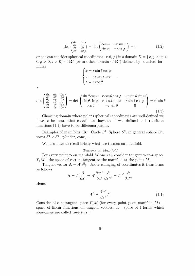
or one can consider spherical coordinates {r, θ, φ} in a domainD = {x, y, z : x >0, y > 0, z > 0} of R3 (or in other domain of R3) defined by standard for-mulae

x = r sin θ cosφ

y = r sin θ sinφ

z = r cos θ

,

,

det

∂x∂r

∂x∂θ

∂x∂φ

∂y∂r

∂y∂θ

∂y∂φ

∂z∂r

∂z∂θ

∂z∂φ

= det

sin θ cosφ r cos θ cosφ −r sin θ sinφsin θ sinφ r cos θ sinφ r sin θ cosφ

cos θ −r sin θ 0

= r2 sin θ

(1.3)Choosing domain where polar (spherical) coordinates are well-defined we

have to be award that coordinates have to be well-defined and transitionfunctions (1.1) have to be diffeomorphisms.

Examples of manifolds: Rn, Circle S1, Sphere S2, in general sphere Sn,torus S1 × S1, cylinder, cone, . . . .

We also have to recall briefly what are tensors on manifold.

Tensors on ManifoldFor every point p on manifold M one can consider tangent vector space

TpM—the space of vectors tangent to the manifold at the point M .Tangent vector A = Ai ∂

∂xi . Under changing of coordinates it transformsas follows:

A = Ai ∂

∂xi= Ai∂x

m′

∂xi

∂

∂xm′ = Am′ ∂

∂xm′

Hence

Ai′ =∂xi′

∂xiAi (1.4)

Consider also cotangent space T ∗pM (for every point p on manifold M)—

space of linear functions on tangent vectors, i.e. space of 1-forms whichsometimes are called covectors.:

5

One-form (covector) ω = ωidxi transforms as follows

ω = ωmdxm = ωm

∂xm

∂xm′ dxm′

= ωm′dxm′.

Hence

ωm′ =∂xm

∂xm′ ωm . (1.5)

Tensors:

One can consider contravariant tensors of the rank p

T = T i1i2...ip∂

∂xi1⊗ ∂

∂xi2⊗ · · · ⊗ ∂

∂xik

with components {T i1i2...ik}.One can consider covariant tensors of the rank q

S = Sj1j2...jqdxj1 ⊗ dxj2 ⊗ . . . dxjq

with components {Sj1j2...jq}.One can also consider mixed tensors:

Q = Qi1i2...ipj1j2...jq

∂

∂xi1⊗ ∂

∂xi2⊗ · · · ⊗ ∂

∂xik⊗ dxj1 ⊗ dxj2 ⊗ . . . dxjq

with components {Qi1i2...ipj1j2...jq

}. We call these tensors tensors of the type

(pq

).

Tensors of the type

(p0

)are called contravariant tensors of the rank p.

Tensors of the type

(0q

)are called covariant tensors of the rank q.

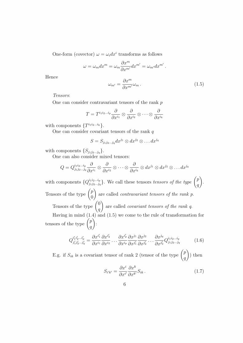
Having in mind (1.4) and (1.5) we come to the rule of transformation for

tensors of the type

(pq

):

Qi′1i

′2...i

′p

j′1j′2...j

′q=

∂xi′1

∂xi1

∂xi′2

∂xi2. . .

∂xi′p

∂xip

∂xj1

∂xj′1

∂xj2

∂xj′2. . .

∂xjq

∂xj′qQ

i1i2...ipj1j2...jq

(1.6)

E.g. if Sik is a covariant tensor of rank 2 (tensor of the type

(pq

)) then

Si′k′ =∂xi

∂xi′

∂xk

∂xk′Sik . (1.7)

6

If Aik is a tensor of rank

(11

)(linear operator on TpM) then

Ai′

k′ =∂xi′

∂xi

∂xk

∂xk′Ai

k

Remark Transformations formulae (1.4)—(1.7) define vectors, covectorsand in generally any tensor fields in components. E.g. covariant tensor (co-variant tensor field) of the rank 2 can be defined as matrix Sik (matrix valuedfunction Sik(x)) such that under changing of coordinates {x1, x2, . . . , xn} 7→{x1′ , x2′ , . . . , xn′} Sik change by the rule (1.7).

Remark Einstein summation rulesIn our lectures we always use so called Einstein summation convention. it

implies that when an index occurs more than once in the same expression inupper and in.. postitions.., the expression is implicitly summed over all pos-sible values for that index. Sometimes it is called dummy indices summationrule.

1.2 Riemannian manifold—manifold equipped with Rie-mannian metric

Definition The Riemannian manifold is a manifold equipped with a Rie-mannian metric.

The Riemannian metric on the manifold M defines the length of thetangent vectors and the length of the curves.

Definition Riemannian metric G on n-dimensional manifold Mn definesfor every point p ∈ M the scalar product of tangent vectors in the tangentspace TpM smoothly depending on the point p.

It means that in every coordinate system (x1, . . . , xn) a metric G =gikdx

idxk is defined by a matrix valued smooth function gik(x) (i = 1, . . . , n; k =1, . . . n) such that for any two vectors

A = Ai(x)∂

∂xi, B = Bi(x)

∂

∂xi,

tangent to the manifoldM at the point p with coordinates x = (x1, x2, . . . , xn)(A,B ∈ TpM) the scalar product is equal to:

⟨A,B⟩G∣∣p= G(A,B)

∣∣p= Ai(x)gik(x)B

k(x) =

7

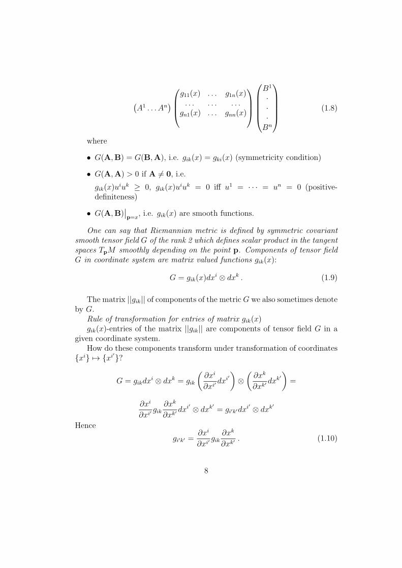
(A1 . . . An

)g11(x) . . . g1n(x). . . . . . . . .

gn1(x) . . . gnn(x)

B1

···Bn

(1.8)

where

• G(A,B) = G(B,A), i.e. gik(x) = gki(x) (symmetricity condition)

• G(A,A) > 0 if A = 0, i.e.

gik(x)uiuk ≥ 0, gik(x)u

iuk = 0 iff u1 = · · · = un = 0 (positive-definiteness)

• G(A,B)∣∣p=x

, i.e. gik(x) are smooth functions.

One can say that Riemannian metric is defined by symmetric covariantsmooth tensor field G of the rank 2 which defines scalar product in the tangentspaces TpM smoothly depending on the point p. Components of tensor fieldG in coordinate system are matrix valued functions gik(x):

G = gik(x)dxi ⊗ dxk . (1.9)

The matrix ||gik|| of components of the metricG we also sometimes denoteby G.

Rule of transformation for entries of matrix gik(x)gik(x)-entries of the matrix ||gik|| are components of tensor field G in a

given coordinate system.How do these components transform under transformation of coordinates

{xi} 7→ {xi′}?

G = gikdxi ⊗ dxk = gik

(∂xi

∂xi′dxi′)⊗(∂xk

∂xk′dxk′

)=

∂xi

∂xi′gik

∂xk

∂xk′dxi′ ⊗ dxk′ = gi′k′dx

i′ ⊗ dxk′

Hence

gi′k′ =∂xi

∂xi′gik

∂xk

∂xk′. (1.10)

8

One can derive transformations formulae also using general formulae (1.7)for tensors.

Important remark

gik =

⟨∂

∂xi,

∂

∂xk

⟩(1.11)

Later by some abuse of notations we sometimes omit the sign of tensorproduct and write a metric just as

G = gik(x)dxidxk .

Examples

• Rn with canonical coordinates {xi} and with metric

G = (dx1)2 + (dx2)2 + · · ·+ (dxn)2

G = ||gik|| = diag [1, 1, . . . , 1]

Recall that this is a basis example of n-dimensional Euclidean space,where scalar product is defined by the formula:

G(X,Y) = ⟨X,Y⟩ = gikXiY k = X1Y 1 +X2Y 2 + · · ·+XnY n .

In the general case if G = ||gik|| is an arbitrary symmetric positive-definite metric then

G(X,Y) = ⟨X,Y⟩ = gikXiY k .

One can show that there exist a new basis {ei} such that in this basis

G(ei, ek) = δik .

This basis is called orthonormal basis. (See the Lecture notes in Ge-ometry)

Scalar product in vector space defines the same scalar product at allthe points. In general case for Riemannian manifold scalar productdepends on the point.

9

• R2 with polar coordinates in the domain y > 0 (x = r cosφ, y =r sinφ):

dx = cosφdr − r sinφdφ, dy = sinφdr + r cosφdφ. In new coordi-nates the Riemannian metric G = dx2 + dy2 will have the followingappearance:

G = (dx)2+(dy)2 = (cosφdr−r sinφdφ)2+(sinφdr+r cosφdφ)2 = dr2+r2(dφ)2

We see that for matrix G = ||gik||

G =

(gxx gxygyx gyy

)=

(1 00 1

)︸︷︷︸in cartesian coordinates

, G =

(grr grφgφr gφφ

)=

(1 00 r

)︸︷︷︸

in polar coordinates

• Circle

Interval [0, 2π) in the line 0 ≤ x < 2π with Riemannian metric

G = a2dx2 (1.12)

Renaming x 7→ φ we come to habitual formula for metric for circle ofthe radius a: x2 + y2 = a2 embedded in the Euclidean space E2:

G = a2dφ2

{x = a cosφ

y = a sinφ, 0 ≤ φ < 2π, (1.13)

• Cylinder surface

Domain in R2 D = {(x, y) : , 0 ≤ x < 2π with Riemannian metric

G = a2dx2 + dy2 (1.14)

We see that renaming variables x 7→ φ, y 7→ h we come to habitual,familiar formulae for metric in standard polar coordinates for cylindersurface of the radius a embedded in the Euclidean space E3:

G = a2dφ2 + dh2

x = a cosφ

y = a sinφ

z = h

, 0 ≤ φ < 2π,−∞ < h < ∞

(1.15)

10

• Sphere

Domain in R2, 0 < x < 2π, 0 < y < π with metric G = dy2 + sin2 ydx2

We see that renaming variables x 7→ φ, y 7→ h we come to habitual,familiar formulae for metric in standard spherical coordinates for spherex2 + y2 + z2 = a2 of the radius a embedded in the Euclidean space E3:

G = a2dθ2+a2 sin2 θdφ2

{x = a sin θ cosφ

y = a sin θ sinφz = a cos θ, 0 ≤ φ < 2π,−∞ < h < ∞

(1.16)

1.2.1 ∗ Pseudoriemannian manifold

If we omit the condition of positive-definiteness for Riemannian metric wecome to so called Pseudorimannian metric. Manifodl equipped with pseu-doriemannan metric is called pseudoriemannian manifold. Pseudoriemannianmanifolds appear in applications in the special and general relativity theory.

Example Consider n+1-dimensional linear space Rn+1 with pseudomet-ric

(dx0)2 − (dx1)2 − (dx2)2 − · · · − (dxn)2

in coordinates x0, x1, . . . , xn. In the case n = 3 it is so called Minkovskispace. The coordinate x0 the role of the time: x0 = ct, where c is the valueof the speed of the light.

1.3 Scalar product. Length of tangent vectors and an-gle between vectors. Length of the curve

The Riemannian metric defines scalar product of tangent vectors attachedat the given point. Hence it defines the length of tangent vectors and anglebetween them. If X = Xm ∂

∂xm ,Y = Y m ∂∂xm are two tangent vectors at the

given point p of Riemannian manifold with coordinates x1, . . . , xn, then wehave that lengths of these vectors equal to

|X| =√

⟨X,X⟩ =√gik(x)X iXk, |Y| =

√⟨Y,Y⟩ =

√gik(x)Y iY k,

(1.17)and he angle θ between these vectors is defined by the relation

cos θ =⟨X,Y⟩|X| · |Y|

=gikX

iY k√gik(x)X iXk

√gik(x)Y iY k

(1.18)

11

Example Let M be 3-dimensional Riemanian manifold. Consider thevectors X = 2∂x+2∂y−∂z and Y = ∂x−2∂y−2∂z attached at the point p ofM with local coordinates (x, y, z), where x = y = 1, z = 0. Find the lengthsof these vectors and angle between them if the expression of Riemannianmetric in these coordinates is coordinates dx2+dy2+dz2

(1+x2+y2)2.

We see that matrix of Riemannian gik = σ(x, y, z)δik, where σ(x, y, z) =1

(1+x2+y2+z2)2δik = 1 if i = k and δik = 0 if i = k, i.e. matrix ||gik|| is

proportional to unity matrix. According to formulae above

|X| =√⟨X,X⟩ =

√gik(x)X iXk =

√σ(x, y, z)

√X iX i = 3

√σ(x, y, z) =

√3 .

The same answer for |Y|. The scalar product between vectors X,Y equal tozero:

⟨X,Y⟩ = σ(x, y, z)δikXiY k = 0

Hence these vectors are orthogonal to each other.

1.3.1 Length of the curve

Let γ : xi = xi(t), (i = 1, . . . , n)) (a ≤ t ≤ b) be a curve on the Riemannianmanifold (M,G).

At the every point of the curve the velocity vector (tangent vector) isdefined:

v(t) =

x1(t)···

xn(t)

(1.19)

The length of velocity vector v ∈ TxM (vector v is tangent to the manifoldM at the point x) equals to

|v|x =√

⟨v,v⟩G∣∣x=√

gikvivk∣∣x=

√gik

dxi(t)

dt

dxk(t)

dt x

∣∣x

(1.20)

The length of the curve is defined by the integral of the length of velocityvector:

Lγ =

∫ b

a

√⟨v,v⟩G

∣∣x(t)

dt =

∫ b

a

√gik(x(t))xi(t)xk(t)dt (1.21)

12

Bearing in mind that metric (1.9) defines the length we often write metricin the following form

ds2 = gikdxidxk (1.22)

For example consider 2-dimensional Riemannian manifold with metric

||gik(u, v)|| =(g11(u, v) g12(u, v)g21(u, v) g22(u, v)

).

Then

G = ds2 = gikduidvk = g11(u, v)du

2 + 2g12(u, v)dudv + g22(u, v)dv2

The length of the curve γ : u = u(t), v = v(t), where t0 ≤ t ≤ t1 according to(1.21) is equal to

Lγ =

∫ t1

t0

√⟨v,v⟩ =

∫ t1

t0

√gik(x)xixk = (1.23)

∫ t1

t0

√g11 (u (t) , v (t))u2

t + 2g12 (u (t) , v (t))utvt + g22 (u (t) , v (t)) v2t dt

(1.24)The length of the curve defined by the formula(1.21) obeys the following

natural conditions

• It coincides with the usual length in the Euclidean space En (Rn withstandard metric G = (dx1)2 + · · · + (dxn)2 in cartesian coordinates).E.g. for 3-dimensional Euclidean space

Lγ =

∫ b

a

√gik(x(t))xi(t)xk(t)dt =

∫ b

a

√(x1(t))2 + (x2(t))2 + (x3(t))2dt

(1.25)

• It does not depend on parameterisation of the curve

Lγ =

∫ b

a


∫ b′

a′

√gik(x(τ))xi(τ)xk(τ)dτ,

(1.26)where xi(τ) = xi(t(τ)), a′ ≤ τ ≤ b′ while a ≤ t ≤ b.

13

• It does not depend on coordinates on Riemannian manifold M

Lγ =

∫ b

a


∫ b

a

√gi′k′(x′(t))xi′(t)xk′(t)dt

(1.27)

• It is additive: if a curve γ = γ1+γ, i.e. γ : xi(t), a ≤ t ≤ b, γ1 : xi(t), a ≤

t ≤ c and γ2 : xi(t), c ≤ t ≤ b where a point c belongs to the interval

(a, b) thenLγ = Lγ1 + Lγ2 , i.e.∫ b

a

√gik(x(t))xi(t)xk(t)dt =∫ c

a

√gik(x(t))xi(t)xk(t)dt+

∫ b

c

√gik(x(t))xi(t)xk(t)dt (1.28)

Conditions (1.25) and (1.28) evidently are obeyed.Condition (1.26) follows from the fact that

xi(τ) =dx(t(τ))

dτ=

dx(t(τ))

dt

dt

dτ= xi(t)

dt

dτ.

Bearing in mind the above formula we have∫ b′

a′

√gik(x(τ))xi(τ)xk(τ)dτ =

∫ b′

a′

√gik(x(t(τ)))xi(t)xk(t)

(dt

dτ

2)dτ =

∫ b′

a′

√gik(x(t(τ)))xi(t)xk(t)

∣∣∣∣ dtdτ∣∣∣∣ dτ =

∫ b

a

√gik(x(t))xi(t)xk(t)dt = Lγ

Condition (1.27) follows from the condition (1.76):∫ b

a

√gi′k′(x′(t))xi′(t)xk′(t)dt =

∫ b

a

√gik(x(t))

∂xi

∂xi′

∂xk

∂xk′xi′(t)xk′(t)dt =

∫ b

a

√gik(x(t))

(∂xi

∂xi′xi′(t)

)(∂xk

∂xk′xk′(t)

)dt =

∫ b

a

√gik(x(t))xi(t)xk(t)dt .

(1.29)

14

1.4 Riemannian structure on the surfaces embeddedin Euclidean space

Let M be a surface embedded in Euclidean space. Let G be Riemannianstructure on the manifold M .

Let X,Y be two vectors tangent to the surface M at a point p ∈ M . AnExternal Observer calculate this scalar product viewing these two vectors asvectors in E3 attached at the point p ∈ E3 using scalar product in E3. AnInternal Observer will calculate the scalar product viewing these two vectorsas vectors tangent to the surface M using the Riemannian metric G (see theformula (1.39)). Respectively

If L is a curve in M then an External Observer consider this curve as acurve in E3, calculate the modulus of velocity vector (speed) and the lengthof the curve using Euclidean scalar product of ambient space. An InternalObserver (”an ant”) will define the modulus of the velocity vector and thelength of the curve using Riemannian metric.

Definition Let M be a surface embedded in the Euclidean space. Wesay that metric GM on the surface is induced by the Euclidean metric if thescalar product of arbitrary two vectors A,B ∈ TpM calculated in terms ofthe metric G equals to Euclidean scalar product of these two vectors:

⟨A,B⟩GM= ⟨A,B⟩GEuclidean

(1.30)

In other words we say that Riemannian metric on the embedded surface isinduced by the Euclidean structure of the ambient space if External andInternal Observers come to the same results calculating scalar product ofvectors tangent to the surface.

In this case modulus of velocity vector (speed) and the length of the curveis the same for External and Internal Observer.

Before going in details of this definition recall the conception of Internaland External Observers when dealing with surfaces in Euclidean space:

1.4.1 Internal and external coordinates of tangent vector

Tangent planeLet r = r(u, v) be parameterisation of the surface M embedded in the Eu-clidean space:

r(u, v) =

x(u, v)y(u, v)z(u, v)

15

Here as always x, y, z are Cartesian coordinates in E3.Let p be an arbitrary point on the surface M . Consider the plane formed

by the vectors which are adjusted to the point p and tangent to the surfaceM . We call this plane plane tangent to M at the point p and denote it byTpM .

For a point p ∈ M one can consider a basis in the tangent plane TpMadjusted to the parameters u, v. Tangent basis vectors at any point (u, v)are

ru =∂r(u, v)

∂u=

∂x(u,v)∂u

∂y(u,v)∂u

∂z(u,v)∂u

=∂x(u, v)

∂u

∂

∂x+

∂y(u, v)

∂u

∂

∂y+

∂z(u, v)

∂u

∂

∂z

Every vector X ∈ TpM can be expanded over this basis:

X = Xuru +Xvrv, (1.31)

where Xu, Xv are coefficients, components of the vector X.Internal Observer views the basis vector ru ∈ TpM , as a velocity vector

for the curve u = u0+ t, v = v0, where (u0, v0) are coordinates of the point p.Respectively the basis vector rv ∈ TpM for an Internal Observer, is velocityvector for the curve u = u0, v = v0 + t, where (u0, v0) are coordinates of thepoint p.

Let r = r(t) be a curve belonging to the surface C, which passes throughthe point p, r(t) = r(u(t), v(t)) and p = r(t0). Then vector

rt =dr

dt=

dr(u(t), v(t))

dt(1.32)

belongs to the tangent plane TpM .Note that for the vector (1.32) components Xu, Xv are equal to Xu =

ut, Xv = vt because

rt =dr

dt=

dr(u(t), v(t))

dt= utru + vtrv (1.33)

An External Observer describes the vector rt as a vector in E3 attached atthe point p. The Internal Observer describes this vector as a vector whichhas components (ut, vt) in the basis ru, rv according to the formula (1.33).

In general consider an arbitrary tangent vector X ∈ TpM . Denote Xu =a, Xv = b

16

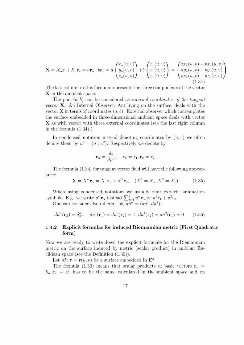
X = Xuru+Xvrv = aru+brv = a

xu(u, v)yu(u, v)zu(u, v)

+b

xv(u, v)xv(u, v)xv(u, v)

=

axu(u, v) + bxv(u, v)ayu(u, v) + byv(u, v)azu(u, v) + bzv(u, v)

(1.34)

The last column in this formula represents the three components of the vectorX in the ambient space.

The pair (a, b) can be considered as internal coordinates of the tangentvector X. An Internal Observer, Ant living on the surface, deals with thevectorX in terms of coordinates (a, b). External observer which contemplatesthe surface embedded in three-dimensional ambient space deals with vectorX as with vector with three external coordinates (see the last right columnin the formula (1.34).)

In condensed notation instead denoting coordinates by (u, v) we oftendenote them by uα = (u1, u2). Respectively we denote by

rα =dr

duα, ru = r1, rv = r2

The formula (1.34) for tangent vector field will have the following appear-ance:

X = Xαrα = X1r1 +X2r2, (X1 = Xu, X2 = Xv) (1.35)

When using condensed notations we usually omit explicit summationsymbols. E.g. we write uαrα instead

∑2i=1 u

αrα or u1r1 + u2r2One can consider also differentials duα = (du1, du2):

duα(rβ) = δαβ : du1(r1) = du2(r2) = 1, du1(r2) = du2(r1) = 0 (1.36)

1.4.2 Explicit formulae for induced Riemannian metric (First Quadraticform)

Now we are ready to write down the explicit formuale for the Riemannianmetric on the surface induced by metric (scalar product) in ambient Eu-clidean space (see the Definition (1.30)).

Let M : r = r(u, v) be a surface embedded in E3.The formula (1.30) means that scalar products of basic vectors ru =

∂u, rv = ∂v has to be the same calculated in the ambient space and on

17

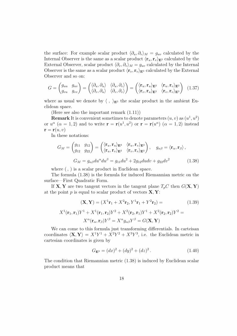
the surface: For example scalar product ⟨∂u, ∂v⟩M = guv calculated by theInternal Observer is the same as a scalar product ⟨ru, rv⟩E3 calculated by theExternal Observer, scalar product ⟨∂v, ∂v⟩M = guv calculated by the InternalObserver is the same as a scalar product ⟨rv, rv⟩E3 calculated by the ExternalObserver and so on:

G =

(guu guvgvu gvv

)=

(⟨∂u, ∂u⟩ ⟨∂u, ∂v⟩⟨∂v, ∂u⟩ ⟨∂v, ∂v⟩

)=

(⟨ru, ru⟩E3 ⟨ru, rv⟩E3

⟨rv, ru⟩E3 ⟨rv, rv⟩E3

)(1.37)

where as usual we denote by ⟨ , ⟩E3 the scalar product in the ambient Eu-clidean space.

(Here see also the important remark (1.11))Remark It is convenient sometimes to denote parameters (u, v) as (u1, u2)

or uα (α = 1, 2) and to write r = r(u1, u2) or r = r(uα) (α = 1, 2) insteadr = r(u, v)

In these notations:

GM =

(g11 g12g12 g22

)=

(⟨ru, ru⟩E3 ⟨ru, rv⟩E3

⟨ru, rv⟩E3 ⟨rv, rv⟩E3

), gαβ = ⟨rα, rβ⟩ ,

GM = gαβduαduβ = g11du

2 + 2g12dudv + g22dv2 (1.38)

where ( , ) is a scalar product in Euclidean space.The formula (1.38) is the formula for induced Riemannian metric on the

surface—First Quadratic Form.If X,Y are two tangent vectors in the tangent plane TpC then G(X,Y)

at the point p is equal to scalar product of vectors X,Y:

(X,Y) = (X1r1 +X2r2, Y1r1 + Y 2r2) = (1.39)

X1(r1, r1)Y1 +X1(r1, r2)Y

2 +X2(r2, r1)Y1 +X2(r2, r2)Y

2 =

Xα(rα, rβ)Yβ = XαgαβY

β = G(X,Y)

We can come to this formula just transforming differentials. In carteisancoordinates ⟨X,Y⟩ = X1Y 1 + X2Y 2 + X3Y 3, i.e. the Euclidean metric incartesian coordinates is given by

GE3 = (dx)2 + (dy)2 + (dz)2 . (1.40)

The condition that Riemannian metric (1.38) is induced by Euclidean scalarproduct means that

18

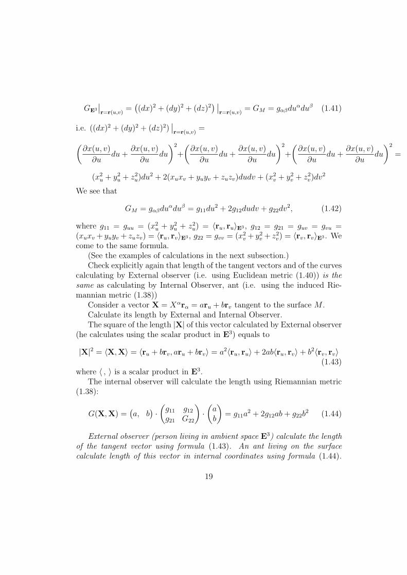
GE3

∣∣r=r(u,v)

=((dx)2 + (dy)2 + (dz)2

) ∣∣r=r(u,v)

= GM = gαβduαduβ (1.41)

i.e. ((dx)2 + (dy)2 + (dz)2)∣∣r=r(u,v)

=(∂x(u, v)

∂udu+

∂x(u, v)

∂udu

)2

+

(∂x(u, v)

∂udu+

∂x(u, v)

∂udu

)2

+

(∂x(u, v)

∂udu+

∂x(u, v)

∂udu

)2

=

(x2u + y2u + z2u)du

2 + 2(xuxv + yuyv + zuzv)dudv + (x2v + y2v + z2v)dv

2

We see that

GM = gαβduαduβ = g11du

2 + 2g12dudv + g22dv2, (1.42)

where g11 = guu = (x2u + y2u + z2u) = ⟨ru, ru⟩E3 , g12 = g21 = guv = gvu =

(xuxv + yuyv + zuzv) = ⟨ru, rv⟩E3 , g22 = gvv = (x2v + y2v + z2v) = ⟨rv, rv⟩E3 . We

come to the same formula.(See the examples of calculations in the next subsection.)Check explicitly again that length of the tangent vectors and of the curves

calculating by External observer (i.e. using Euclidean metric (1.40)) is thesame as calculating by Internal Observer, ant (i.e. using the induced Rie-mannian metric (1.38))

Consider a vector X = Xαrα = aru + brv tangent to the surface M .Calculate its length by External and Internal Observer.The square of the length |X| of this vector calculated by External observer

(he calculates using the scalar product in E3) equals to

|X|2 = ⟨X,X⟩ = ⟨ru + brv, aru + brv⟩ = a2⟨ru, ru⟩+ 2ab⟨ru, rv⟩+ b2⟨rv, rv⟩(1.43)

where ⟨ , ⟩ is a scalar product in E3.The internal observer will calculate the length using Riemannian metric

(1.38):

G(X,X) =(a, b

)·(g11 g12g21 G22

)·(ab

)= g11a

2 + 2g12ab+ g22b2 (1.44)

External observer (person living in ambient space E3) calculate the lengthof the tangent vector using formula (1.43). An ant living on the surfacecalculate length of this vector in internal coordinates using formula (1.44).

19

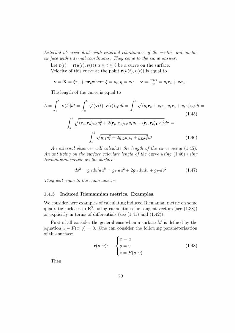
External observer deals with external coordinates of the vector, ant on thesurface with internal coordinates. They come to the same answer.

Let r(t) = r(u(t), v(t)) a ≤ t ≤ b be a curve on the surface.Velocity of this curve at the point r(u(t), v(t)) is equal to

v = X = ξru + ηrvwhere ξ = ut, η = vt : v = dr(t)dt

= utru + vtrv .

The length of the curve is equal to

L =

∫ b

a

|v(t)|dt =∫ b

a

√⟨v(t),v(t)⟩E3dt =

∫ b

a

√⟨utru + vtrv, utru + vtrv⟩E3dt =

(1.45)∫ b

a

√⟨ru, ru⟩E3u2

t + 2⟨ru, rv⟩E3utvt + ⟨rv, rv⟩E3v2t dτ =∫ b

a

√g11u2

t + 2g12utvt + g22v2t dt (1.46)

An external observer will calculate the length of the curve using (1.45).An ant living on the surface calculate length of the curve using (1.46) usingRiemannian metric on the surface:

ds2 = gikduiduk = g11du

2 + 2g12dudv + g22dv2 (1.47)

They will come to the same answer.

1.4.3 Induced Riemannian metrics. Examples.

We consider here examples of calculating induced Riemanian metric on somequadratic surfaces in E3. using calculations for tangent vectors (see (1.38))or explicitly in terms of differentials (see (1.41) and (1.42)).

First of all consider the general case when a surface M is defined by theequation z − F (x, y) = 0. One can consider the following parameterisationof this surface:

r(u, v) :

x = u

y = v

z = F (u, v)

(1.48)

Then

20

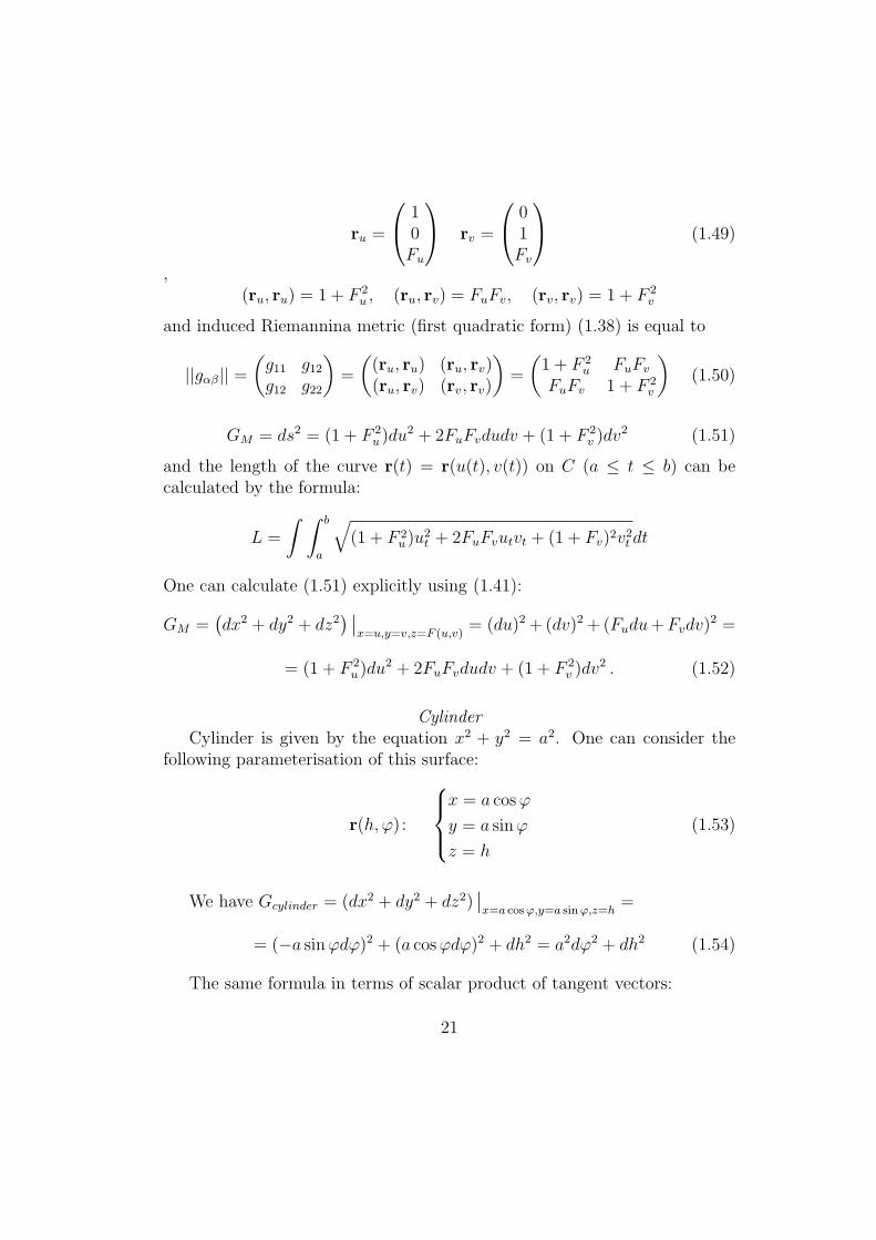
ru =

10Fu

rv =

01Fv

(1.49)

,(ru, ru) = 1 + F 2

u , (ru, rv) = FuFv, (rv, rv) = 1 + F 2v

and induced Riemannina metric (first quadratic form) (1.38) is equal to

||gαβ|| =(g11 g12g12 g22

)=

((ru, ru) (ru, rv)(ru, rv) (rv, rv)

)=

(1 + F 2

u FuFv

FuFv 1 + F 2v

)(1.50)

GM = ds2 = (1 + F 2u )du

2 + 2FuFvdudv + (1 + F 2v )dv

2 (1.51)

and the length of the curve r(t) = r(u(t), v(t)) on C (a ≤ t ≤ b) can becalculated by the formula:

L =

∫ ∫ b

a

√(1 + F 2

u )u2t + 2FuFvutvt + (1 + Fv)2v2t dt

One can calculate (1.51) explicitly using (1.41):

GM =(dx2 + dy2 + dz2

) ∣∣x=u,y=v,z=F (u,v)

= (du)2 +(dv)2 +(Fudu+Fvdv)2 =

= (1 + F 2u )du

2 + 2FuFvdudv + (1 + F 2v )dv

2 . (1.52)

CylinderCylinder is given by the equation x2 + y2 = a2. One can consider the

following parameterisation of this surface:

r(h, φ) :

x = a cosφ

y = a sinφ

z = h

(1.53)

We have Gcylinder = (dx2 + dy2 + dz2)∣∣x=a cosφ,y=a sinφ,z=h

=

= (−a sinφdφ)2 + (a cosφdφ)2 + dh2 = a2dφ2 + dh2 (1.54)

The same formula in terms of scalar product of tangent vectors:

21

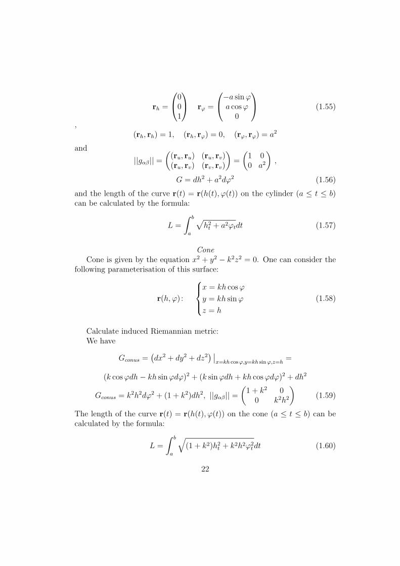
rh =

001

rφ =

−a sinφa cosφ

0

(1.55)

,(rh, rh) = 1, (rh, rφ) = 0, (rφ, rφ) = a2

and

||gαβ|| =((ru, ru) (ru, rv)(ru, rv) (rv, rv)

)=

(1 00 a2

),

G = dh2 + a2dφ2 (1.56)

and the length of the curve r(t) = r(h(t), φ(t)) on the cylinder (a ≤ t ≤ b)can be calculated by the formula:

L =

∫ b

a

√h2t + a2φtdt (1.57)

ConeCone is given by the equation x2 + y2 − k2z2 = 0. One can consider the

following parameterisation of this surface:

r(h, φ) :

x = kh cosφ

y = kh sinφ

z = h

(1.58)

Calculate induced Riemannian metric:We have

Gconus =(dx2 + dy2 + dz2

) ∣∣x=kh cosφ,y=kh sinφ,z=h

=

(k cosφdh− kh sinφdφ)2 + (k sinφdh+ kh cosφdφ)2 + dh2

Gconus = k2h2dφ2 + (1 + k2)dh2, ||gαβ|| =(1 + k2 0

0 k2h2

)(1.59)

The length of the curve r(t) = r(h(t), φ(t)) on the cone (a ≤ t ≤ b) can becalculated by the formula:

L =

∫ b

a

√(1 + k2)h2

t + k2h2φ2tdt (1.60)

22

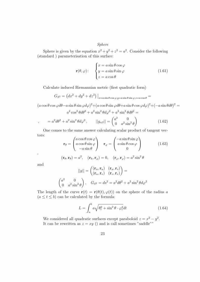
Sphere

Sphere is given by the equation x2 + y2 + z2 = a2. Consider the following(standard ) parameterisation of this surface:

r(θ, φ) :

x = a sin θ cosφ

y = a sin θ sinφ

z = a cos θ

(1.61)

Calculate induced Riemannian metric (first quadratic form)

GS2 =(dx2 + dy2 + dz2

) ∣∣x=a sin θ cosφ,y=a sin θ sinφ,z=a cos θ

=

(a cos θ cosφdθ−a sin θ sinφdφ)2+(a cos θ sinφdθ+a sin θ cosφdφ)2+(−a sin θdθ)2 =

a2 cos2 θdθ2 + a2 sin2 θdφ2 + a2 sin2 θdθ2 =

, = a2dθ2 + a2 sin2 θdφ2 , ||gαβ|| =(a2 00 a2 sin2 θ

)(1.62)

One comes to the same answer calculating scalar product of tangent vec-tors:

rθ =

a cos θ cosφa cos θ sinφ−a sin θ

rφ =

−a sin θ sinφa sin θ cosφ

0

(1.63)

,(rθ, rθ) = a2, (rh, rφ) = 0, (rφ, rφ) = a2 sin2 θ

and

||g|| =((ru, ru) (ru, rv)(ru, rv) (rv, rv)

)=(

a2 00 a2 sin2 θ

), GS2 = ds2 = a2dθ2 + a2 sin2 θdφ2

The length of the curve r(t) = r(θ(t), φ(t)) on the sphere of the radius a(a ≤ t ≤ b) can be calculated by the formula:

L =

∫ b

a

a

√θ2t + sin2 θ · φ2

tdt (1.64)

We considered all quadratic surfaces except paraboloid z = x2 − y2.It can be rewritten as z = xy () and is call sometimes ”saddle””

23

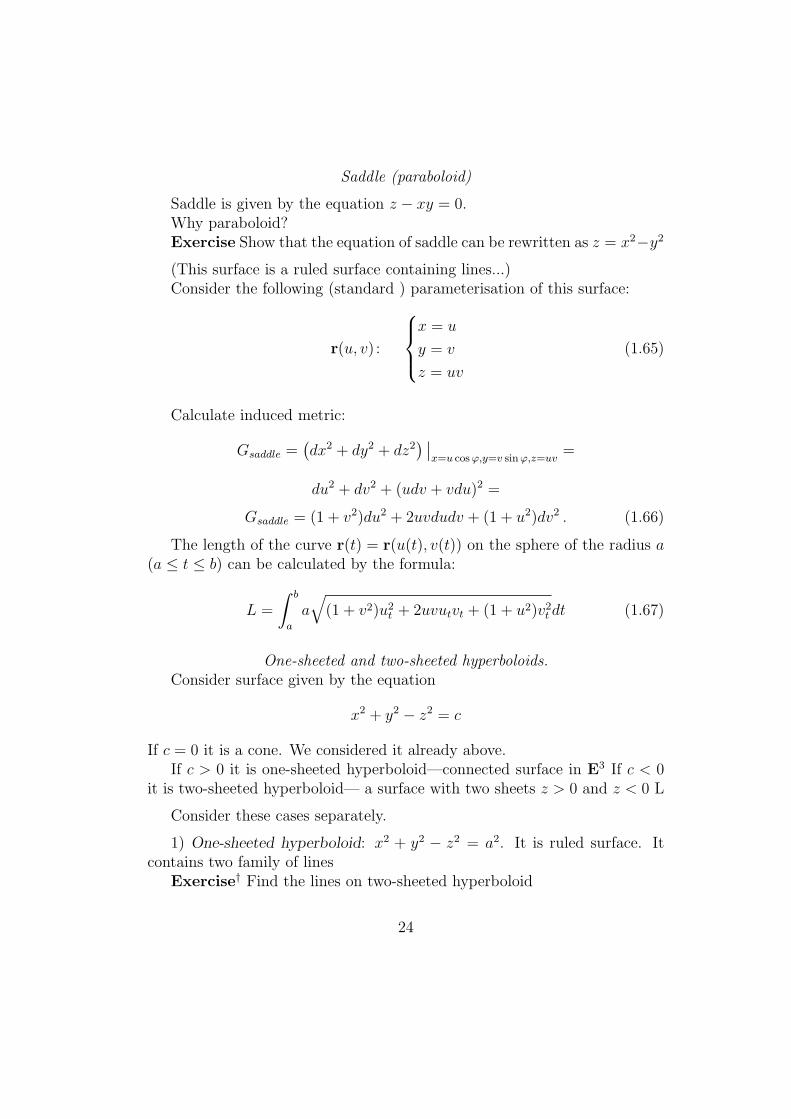
Saddle (paraboloid)

Saddle is given by the equation z − xy = 0.Why paraboloid?Exercise Show that the equation of saddle can be rewritten as z = x2−y2

(This surface is a ruled surface containing lines...)Consider the following (standard ) parameterisation of this surface:

r(u, v) :

x = u

y = v

z = uv

(1.65)

Calculate induced metric:

Gsaddle =(dx2 + dy2 + dz2

) ∣∣x=u cosφ,y=v sinφ,z=uv

=

du2 + dv2 + (udv + vdu)2 =

Gsaddle = (1 + v2)du2 + 2uvdudv + (1 + u2)dv2 . (1.66)

The length of the curve r(t) = r(u(t), v(t)) on the sphere of the radius a(a ≤ t ≤ b) can be calculated by the formula:

L =

∫ b

a

a√(1 + v2)u2

t + 2uvutvt + (1 + u2)v2t dt (1.67)

One-sheeted and two-sheeted hyperboloids.Consider surface given by the equation

x2 + y2 − z2 = c

If c = 0 it is a cone. We considered it already above.If c > 0 it is one-sheeted hyperboloid—connected surface in E3 If c < 0

it is two-sheeted hyperboloid— a surface with two sheets z > 0 and z < 0 L

Consider these cases separately.

1) One-sheeted hyperboloid: x2 + y2 − z2 = a2. It is ruled surface. Itcontains two family of lines

Exercise† Find the lines on two-sheeted hyperboloid

24

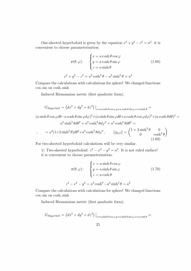
One-sheeted hyperboloid is given by the equation x2 + y2 − z2 = a2. it isconvenient to choose parameterisation:

r(θ, φ) :

x = a cosh θ cosφ

y = a cosh θ sinφ

z = a sinh θ

(1.68)

x2 + y2 − z2 = a2 cosh2 θ − a2 sinh2 θ = a2

Compare the calculations with calculations for sphere! We changed functionscos, sin on cosh, sinh

Induced Riemannian metric (first quadratic form).

GHyperbolI =(dx2 + dy2 + dz2

) ∣∣x=a cosh θ cosφ,y=a cosh θ sinφ,z=a sinh θ

=

(a sinh θ cosφdθ−a cosh θ sinφdφ)2+(a sinh θ sinφdθ+a cosh θ cosφdφ)2+(a cosh θdθ)2 =

a2 sinh2 θdθ2 + a2 cosh2 θdφ2 + a2 cosh2 θdθ2 =

, = a2(1+2 sinh2 θ)dθ2+a2 cosh2 θdφ2 , ||gαβ|| =(1 + 2 sinh2 θ 0

0 cosh2 θ

)(1.69)

For two-sheeted hyperboloid calculatiosn will be very similar.

1) Two-sheeted hyperboloid: z2 − x2 − y2 = a2. It is not ruled surface!it is convenient to choose parameterisation:

r(θ, φ) :

x = a sinh θ cosφ

y = a sinh θ sinφ

z = a cosh θ

(1.70)

z2 − x2 − y2 = a2 coshθ −a2 sinh2 θ = a2

Compare the calculations with calculations for sphere! We changed functionscos, sin on cosh, sinh

Induced Riemannian metric (first quadratic form).

GHyperbolI =(dx2 + dy2 + dz2

) ∣∣x=a sinh θ cosφ,y=a sinh θ sinφ,z=a cosh θ

=

25

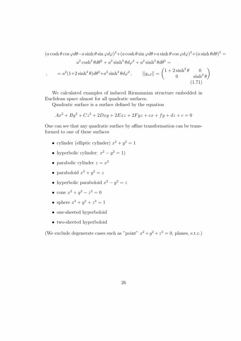
(a cosh θ cosφdθ−a sinh θ sinφdφ)2+(a cosh θ sinφdθ+a sinh θ cosφdφ)2+(a sinh θdθ)2 =

a2 cosh2 θdθ2 + a2 sinh2 θdφ2 + a2 sinh2 θdθ2 =

, = a2(1+2 sinh2 θ)dθ2+a2 sinh2 θdφ2 , ||gαβ|| =(1 + 2 sinh2 θ 0

0 sinh2 θ

)(1.71)

We calculated examples of induced Riemannian structure embedded inEuclidean space almost for all quadratic surfaces.

Quadratic surface is a surface defined by the equation

Ax2 +By2 + Cz2 + 2Dxy + 2Exz + 2Fyz + ex+ fy + dz + c = 0

One can see that any quadratic surface by affine transformation can be trans-formed to one of these surfaces

• cylinder (elliptic cylinder) x2 + y2 = 1

• hyperbolic cylinder: x2 − y2 = 1)

• parabolic cylinder z = x2

• paraboloid x2 + y2 = z

• hyperbolic paraboloid x2 − y2 = z

• cone x2 + y2 − z2 = 0

• sphere x2 + y2 + z2 = 1

• one-sheeted hyperboloid

• two-sheeted hyperboloid

(We exclude degenerate cases such as ”point” x2+y2+ z2 = 0, planes, e.t.c.)

26

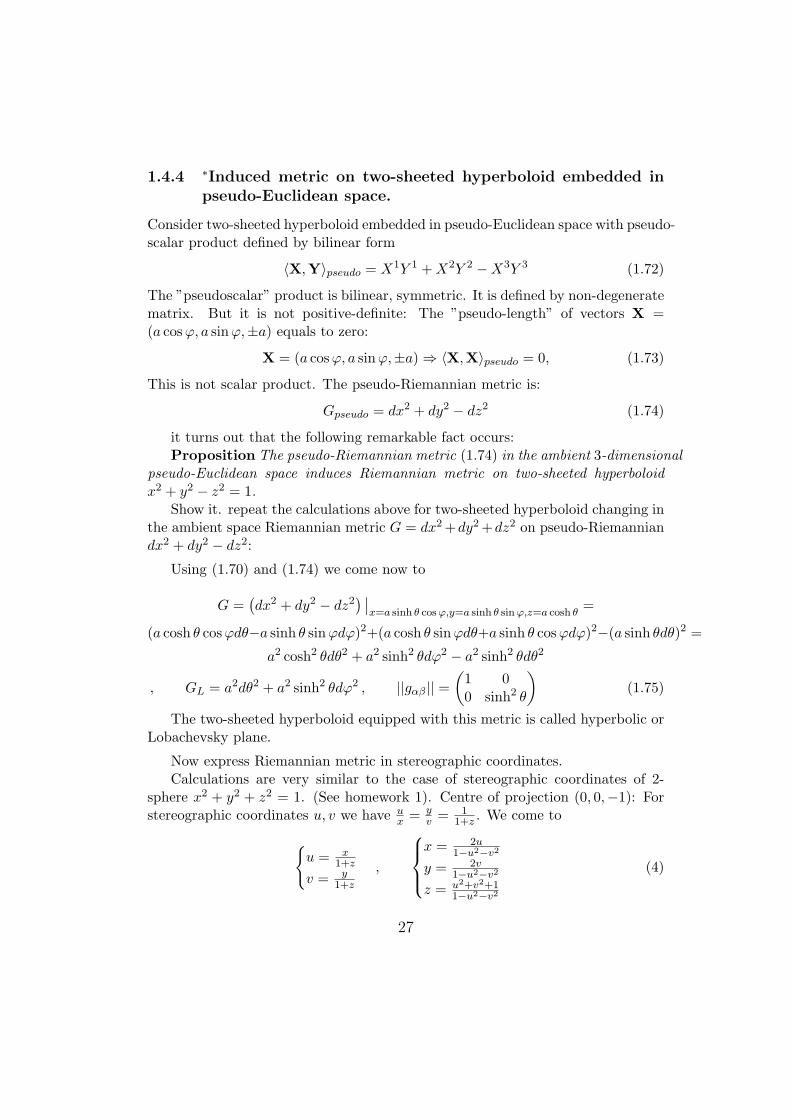
1.4.4 ∗Induced metric on two-sheeted hyperboloid embedded inpseudo-Euclidean space.

Consider two-sheeted hyperboloid embedded in pseudo-Euclidean space with pseudo-scalar product defined by bilinear form

⟨X,Y⟩pseudo = X1Y 1 +X2Y 2 −X3Y 3 (1.72)

The ”pseudoscalar” product is bilinear, symmetric. It is defined by non-degeneratematrix. But it is not positive-definite: The ”pseudo-length” of vectors X =(a cosφ, a sinφ,±a) equals to zero:

X = (a cosφ, a sinφ,±a) ⇒ ⟨X,X⟩pseudo = 0, (1.73)

This is not scalar product. The pseudo-Riemannian metric is:

Gpseudo = dx2 + dy2 − dz2 (1.74)

it turns out that the following remarkable fact occurs:Proposition The pseudo-Riemannian metric (1.74) in the ambient 3-dimensional

pseudo-Euclidean space induces Riemannian metric on two-sheeted hyperboloidx2 + y2 − z2 = 1.

Show it. repeat the calculations above for two-sheeted hyperboloid changing inthe ambient space Riemannian metric G = dx2+dy2+dz2 on pseudo-Riemanniandx2 + dy2 − dz2:

Using (1.70) and (1.74) we come now to

G =(dx2 + dy2 − dz2

) ∣∣x=a sinh θ cosφ,y=a sinh θ sinφ,z=a cosh θ

=

(a cosh θ cosφdθ−a sinh θ sinφdφ)2+(a cosh θ sinφdθ+a sinh θ cosφdφ)2−(a sinh θdθ)2 =

a2 cosh2 θdθ2 + a2 sinh2 θdφ2 − a2 sinh2 θdθ2

, GL = a2dθ2 + a2 sinh2 θdφ2 , ||gαβ || =(1 00 sinh2 θ

)(1.75)

The two-sheeted hyperboloid equipped with this metric is called hyperbolic orLobachevsky plane.

Now express Riemannian metric in stereographic coordinates.Calculations are very similar to the case of stereographic coordinates of 2-

sphere x2 + y2 + z2 = 1. (See homework 1). Centre of projection (0, 0,−1): Forstereographic coordinates u, v we have u

x = yv = 1

1+z . We come to

{u = x

1+z

v = y1+z

,

x = 2u

1−u2−v2

y = 2v1−u2−v2

z = u2+v2+11−u2−v2

(4)

27

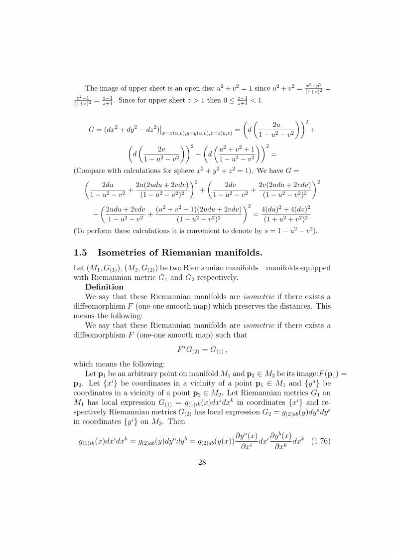
The image of upper-sheet is an open disc u2 + v2 = 1 since u2 + v2 = x2+y2

(1+z)2=

z2−1(1+z)2

= z−1z+1 . Since for upper sheet z > 1 then 0 ≤ z−1

z+1 < 1.

G = (dx2 + dy2 − dz2)∣∣x=x(u,v),y=y(u,v),z=z(u,v)

=

(d

(2u

1− u2 − v2

))2

+

(d

(2v

1− u2 − v2

))2

−(d

(u2 + v2 + 1

1− u2 − v2

))2

=

(Compare with calculations for sphere x2 + y2 + z2 = 1). We have G =(2du

1− u2 − v2+

2u(2udu+ 2vdv)

(1− u2 − v2)2

)2

+

(2dv

1− u2 − v2+

2v(2udu+ 2vdv)

(1− u2 − v2)2

)2

−(2udu+ 2vdv

1− u2 − v2+

(u2 + v2 + 1)(2udu+ 2vdv)

(1− u2 − v2)2

)2

=4(du)2 + 4(dv)2

(1 + u2 + v2)2

(To perform these calculations it is convenient to denote by s = 1− u2 − v2).

1.5 Isometries of Riemanian manifolds.

Let (M1, G(1)), (M2, G(2)) be two Riemannian manifolds—manifolds equippedwith Riemannian metric G1 and G2 respectively.

DefinitionWe say that these Riemannian manifolds are isometric if there exists a

diffeomorphism F (one-one smooth map) which preserves the distances. Thismeans the following:

We say that these Riemannian manifolds are isometric if there exists adiffeomorphism F (one-one smooth map) such that

F ∗G(2) = G(1) ,

which means the following:Let p1 be an arbitrary point on manifoldM1 and p2 ∈ M2 be its image:F (p1) =

p2. Let {xi} be coordinates in a vicinity of a point p1 ∈ M1 and {ya} becoordinates in a vicinity of a point p2 ∈ M2. Let Riemannian metrics G1 onM1 has local expression G(1) = g(1)ik(x)dx

idxk in coordinates {xi} and re-spectively Riemannian metrics G(2) has local expression G2 = g(2)ab(y)dy

adyb

in coordinates {yi} on M2. Then

g(1)ik(x)dxidxk = g(2)ab(y)dy

adyb = g(2)ab(y(x))∂ya(x)

∂xidxi∂y

b(x)

∂xkdxk (1.76)

28

i.e.

g(1)ik(x) =∂ya(x)

∂xig(2)ab(y(x))

∂yb(x)

∂xk. (1.77)

where yi = yi(x) is local expression for diffeomorphism F .

Definition We say that two Riemannian manifolds (M1, G(1)), (M2, G(2))are locally isometric if the following conditions hold:

For arbitrary point p1 on the manifold M1 there exists a point p2 on themanifold M2 such that there exist coordinates {xi} in a vicinity of a pointp1 ∈ M1 and coordinates {ya} in a vicinity of a point p2 ∈ M2 such that localexpression for metric G(1) on M1 in coordinates {xi} and local expression formetric G(2) on M2 in coordinates {ya} are related via formuale (1.76), (1.29).

Locally isometric Riemannian manifolds have not to be diffeomorphic.E.g. Euclidean plane is locally isometric to cylinder, but they are not diffeo-morphic.

1.5.1 Examples of local isometries

Consider examples.

Example 1 Cylinder-Cone—Plane,Riemannian metric on cylinder is Gcylinder = a2dφ2+dh2 and on the cone

Gconus = k2h2dφ2 + (1 + k2)dh2 (see formulae (1.54) and (1.59)).To show that cylinder is isometric to Euclidean plan we have to find

new local coordinates u, v on the cylinder such that in these coordinates themetric on the cylinder equals to du2 + dv2. If we put u = aφ, v = h then

du2 + dv2 = d(aφ)2 + dh2 = a2dφ2 + dh2 = Gcylinder . (1.78)

Thus we prove the local isometry. Of course the coordinate u = φ is notglobal coordinate on the surface of cylinder. It is evident that cylinder andplane are not globally isometric since there are no diffeomorphism of cylinderon the plane. (They are different non-homeomorphic topological spaces.)

Now show that cone is locally isometric to the plane.This means that we have to find local coordinates u, v on the cone such

that in these coordinates induced metric G|c on cone would have the appear-ance G|c = du2 + dv2.

29

First of all calculate the metric on cone in natural coordinates h, φ where

r(h, φ) :

x = kh cosφ

y = kh sinφ

z = h

.

(x2 + y2 − k2z2 = k2h2 cos2 φ+ k2h2 sin2 φ− k2h2 = k2h2 − k2h2 = 0.Calculate metric Gc on the cone in coordinates h, φ induced with the

Euclidean metric G = dx2 + dy2 + dz2:

Gc =(dx2 + dy2 + dz2


= (k cosφdh− kh sinφdφ)2+

(k sinφdh+ kh cosφdφ)2 + dh2 = (k2 + 1)dh2 + k2h2dφ2 .

In analogy with polar coordinates try to find new local coordinates u, v such

that

{u = αh cos βφ

v = αh sin βφ, where α, β are parameters. We come to du2+dv2 =

(α cos βφdh− αβh sin βφdφ)2+(α sin βφdh+ αβh cos βφdφ)2 = α2dh2+α2β2h2dφ2.

Comparing with the metric on the cone Gc = (1 + k2)dh2 + k2h2dφ2 we seethat if we put α = k and β = k√

1+k2then du2 + dv2 = α2dh2 + α2β2h2dφ2 =

(1 + k2)dh2 + k2h2dφ2.Thus in new local coordinates{

u =√k2 + 1h cos k√

k2+1φ

v =√k2 + 1h sin k√

k2+1φ

induced metric on the cone becomes G|c = du2 + dv2, i.e. cone locally isisometric to the Euclidean plane

Of course these coordinates are local.— Cone and plane are not homeo-morphic, thus they are not globally isometric.

One can show also that2) Plane with metric 4R2(dx2+dy2)

(1+x2+y2)2is isometric to the sphere with radius

R(a) = ...3) Disc with metric du2+dv2

(1−u2−v2)2is isometric to half plane with metric

dx2+dy2

4y2.

(see exercises in Homeworks and Coursework.)

30

1.6 Volume element in Riemannian manifold

The volume element in n-dimensional Riemannian manifold with metric G =gikdx

idxk is defined by the formula√det gik dx

1dx2 . . . dxn (1.79)

If D is a domain in the n-dimensional Riemannian manifold with metricG = gikdx

i then its volume is equal to to the integral of volume element overthis domain.

V (D) =

∫D

√det gik dx

1dx2 . . . dxn (1.80)

Remark Students who know the concept of exterior forms can read thevolume element as √

det gik dx1 ∧ dx2 ∧ · · · ∧ dxn (1.81)

Note that in the case of n = 1 volume is just the length, in the case ifn = 2 it is area.

1.6.1 Volume of parallelepiped

Note that the formula (1.79) gives the volume of n-dimensional parallelepiped.Show this. Let En be Euclidean vector space with orthonormal basis {ei}.Let vi be an arbitrary basis in this vector space (vectors vi in general have notunit length and are not orthogonal to each other). Consider n-parallelepipedspanned by vectors {vi}:

Πvi: r = tivi, 0 ≤ ti ≤ 1.

The volume of this parallelepiped equals to

V ol(Πvi) = det ||ami || , (1.82)

where A = ||ami || is transition matrix, vi = emami . On the other hand

r = xiei = tmvm, hence xi = aimtm, where vm = eia

im.

Let G = (dx1)2 + · · · + (dxn)2 = gikdtidtk be usual Euclidean metric in new

coordinates ti. The

G = (dx1)2 + · · ·+ (dxn)2 = dxiδikdxk = dti

∂xi′

∂tiδi′k′

∂xk′

∂tkdtk.

31

Since ∂xi′

∂ti= ai

′i then

gik =∑i′

ai′

i ai′

k ⇒ det g = (detA)2, det g =√detA.

and according to the formula (1.80)

V ol(Πvi) =

∫0≤ti≤1

√det gdt1dt2 . . . dtn = detA .

We come to (1.82).

Perform these calculations in detail for 3-dimensional case.E.g. if Euclidean space is 3-dimensional then the parallelepiped spanned

by basis vectors {a,b, c}

Πa,b,c = t1a+ t2b+ t3c , 0 ≤ t1, t2, t3 ≤ 1.

Volume of parallelepiped equals to

V olΠa,b,c = det

ax bx cxay by cyaz bz cz

, (1.83)

and xyz

=


t1

t2

t3

.

The Riemannian metric in new coordinates (t1, t2, t3) equals to

dx2 + dy2 + dz2 =(dt1 dt2 dt3

)ax ay azbx by bzcx cy cz


dt1

dt2

dt3

,

i.e. in coordinates ti Riemannian metric G = gikdtidtk whereg11 g12 g13

g21 g22 g23g31 g32 g33

=

ax ay azbx by bzcx cy cz


i.e. √

det gik = det


= V olΠa,b,c . (1.84)

32

1.6.2 Invariance of volume element under changing of coordinates

Prove that volume element is invariant under coordinate transformations, i.e. ify1, . . . , yn are new coordinates: x1 = x1(y1, . . . , yn), x2 = x2(y1, . . . , yn)...,

xi = xi(yp), i = 1, . . . , n , p = 1, . . . , n

and gpq(y) matrix of the metric in new coordinates:

gpq(y) =∂xi

∂ypgik(x(y))

∂xk

∂yq. (1.85)

Then √det gik(x) dx

1dx2 . . . dxn =√

det gpq(y) dy1dy2 . . . dyn (1.86)

This follows from (1.85). Namely

√det gik(y) dy

1dy2 . . . dyn =

√det

(∂xi

∂ypgik(x(y))

∂xk

∂yq

)dy1dy2 . . . dyn

Using the fact that det(ABC) = detA · detB · detC and det(

∂xi

∂yp

)= det

(∂xk

∂yq

)1

we see that from the formula above follows:√det gik(y) dy

1dy2 . . . dyn =

√det

(∂xi

∂ypgik(x(y))

∂xk

∂yq

)dy1dy2 . . . dyn =

√(det

(∂xi

∂yp

))2√det gik(x(y))dy

1dy2 . . . dyn =

√det gik(x(y)) det

(∂xi

∂yp

)dy1dy2 . . . dyn = (1.87)

Now note that

det

(∂xi

∂yp

)dy1dy2 . . . dyn = dx1 . . . dxn

according to the formula for changing coordinates in n-dimensional integral 2.Hence√

det gik(x(y)) det

(∂xi

∂yp

)dy1dy2 . . . dyn =

√det gik(x(y))dx

1dx2 . . . dxn (1.88)

1determinant of matrix does not change if we change the matrix on the adjoint, i.e.change columns on rows.

2Determinant of the matrix(

∂xi

∂yp

)of changing of coordinates is called sometimes Ja-

cobian. Here we consider the case if Jacobian is positive. If Jacobian is negative thenformulae above remain valid just the symbol of modulus appears.

33

Thus we come to (1.86).

1.6.3 Examples of calculating volume element

Consider first very simple example: Volume element of plane in cartesiancoordinates, metric g = dx2 + dy2. Volume element is equal to

√det gdxdy =

√det

(1 00 1

)dxdy = dxdy

Volume of the domain D is equal to

V (D) =

∫D

√det gdxdy =

∫D

dxdy

If we go to polar coordinates:

x = r cosφ, y = r sinφ (1.89)

Then we have for metric:G = dr2 + r2dφ2

because

dx2 + dy2 = (dr cosφ− r sinφdφ)2 + (dr sinφ+ r cosφdφ)2 = dr2 + r2dφ2

(1.90)Volume element in polar coordinates is equal to

√det gdrdφ =

√det

(1 00 r2

)drdφ = drdφ .

Lobachesvky plane.In coordinates x, y (y > 0) metric G = dx2+dy2

y2, the corresponding matrix

G =

(1/y2 0

0 1/y2

). Volume element is equal to

√det gdxdy = dxdy

y2.

Sphere in stereographic coordinates Consider the two dimensional planewith Riemannian metrics

G =4R2(du2 + dv2)

(1 + u2 + v2)2(1.91)

34

(It is isometric to the sphere of the radius R without North pole in stere-ographic coordinates (see the Homeworks.))

Calculate its volume element and volume. It is easy to see that:

G =

(4R2

(1+u2+v2)20

0 4R2

(1+u2+v2)2

)det g =

16R4

(1 + u2 + v2)4(1.92)

and volume element is equal to√det gdudv = 4R2dudv

(1+u2+v2)2

One can calculate volume in coordinates u, v but it is better to considervolume form in polar coordinates u = r cosφ, v = r sinφ. Then it is easy

to see that according to (1.90) we have for the metric G = R2(du2+dv2)(1+u2+v2)2

=R2(dr2+r2dφ2)

(1+r2)2and volume form is equal to

√det gdrdφ = 4R2rdrdφ

(1+r2)2

Now calculation of integral becomes easy:

V =

∫4R2rdrdφ

(1 + r2)2= 8πR2

∫ ∞

0

rdr

(1 + r2)2= 4πR2

∫ ∞

0

du

(1 + u)2= 4πR2 .

Segment of the sphere.Consider sphere of the radius a in Euclidean space with standard Riema-

nian metrica2dθ2 + a2 sin2 θdφ2

This metric is nothing but first quadratic form on the sphere (see (1.4.3)).The volume element is

√det gdθdφ =

√det

(a2 00 a2 sin θ

)dθdφ = a2 sin θdθdφ

Now calculate the volume of the segment of the sphere between two parallelplanes, i.e. domain restricted by parallels θ1 ≤ θ ≤ θ0: Denote by h be theheight of this segment. One can see that

h = a cos θ0 − a cos θ1 = a(cos θ0 − a cos θ1)

There is remarkable formula which express the area of segment via the heighth:

V =

∫θ1≤θ≤θ0

(a2 sin θ

)dθdφ =

∫ θ1

θ0

(∫ 2π

0

(a2 sin θ

)dφ

)dθ =

35

∫ θ0

θ12πa2 sin θdθ = 2πa2(cos θ0 − cos θ1) = 2πa(a cos θ0 − acosθ1) = 2πah

(1.93)E.g. for all the sphere h = 2a. We come to S = 4πa2. It is remarkableformula: area of the segment is a polynomial function of radius of the sphereand height (Compare with formula for length of the arc of the circle)

2 Covariant differentiaion. Connection. Levi

Civita Connection on Riemannian mani-

fold

2.1 Differentiation of vector field along the vector field.—Affine connection

How to differentiate vector fields on a (smooth )manifold M?Recall the differentiation of functions on a (smooth )manifold M .Let X = Xi(x)ei(x) = ∂

∂xi be a vector field on M . Recall that vectorfield 3 X = Xiei defines at the every point x0 an infinitesimal curve: xi(t) =xi0 + tX i (More exactly the equivalence class [γ(t)]X of curves xi(t) = xi

0 +tX i + . . . ).

Let f be an arbitrary (smooth) function on M and X = X i ∂∂xi . Then

derivative of function f along vector field X = X i ∂∂xi is equal to

∂Xf = ∇Xf = X i ∂f

∂xi

The geometrical meaning of this definition is following: If X is a velocityvector of the curve xi(t) at the point xi

0 = xi(t) at the ”time” t = 0 thenthe value of the derivative ∇Xf at the point xi

0 = xi(0) is equal just to thederivative by t of the function f(xi(t)) at the ”time” t = 0:

if X i(x)∣∣x0=x(0)

=dxi(t)

dt

∣∣t=0

, then ∇Xf∣∣xi=xi(0)

=d

dtf(xi (t)

) ∣∣t=0

(2.1)Remark In the course of Geometry and Differentiable Manifolds the

operator of taking derivation of function along the vector field was denoted

3here like always we suppose by default the summation over repeated indices. E.g.X =Xiei is nothing but X =

∑ni=1 X

iei

36

by ”∂Xf”. In this course we prefer to denote it by ”∇Xf” to have the uniformnotation for both operators of taking derivation of functions and vector fieldsalong the vector field.

One can see that the operation∇X on the space C∞(M) (space of smoothfunctions on the manifold) satisfies the following conditions:

• ∇X (λf + µg) = a∇Xf+b∇Xg where λ, µ ∈ R (linearity over numbers)

• ∇hX+gY(f) = h∇X(f)+ g∇Y(f) (linearity over the space of functions)

• ∇X(λfg) = f∇X(λg) + g∇X(λf) (Leibnitz rule)

(2.2)

RemarkOne can prove that these properties characterize vector fields:operatoron smooth functions obeying the conditions above is a vector field. (You willhave a detailed analysis of this statement in the course of Differentiable Man-ifolds.)

How to define differentiation of vector fields along vector fields.The formula (2.1) cannot be generalised straightforwardly because vec-

tors at the point x0 and x0 + tX are vectors from different vector spaces.(We cannot substract the vector from one vector space from the vector fromthe another vector space, because apriori we cannot compare vectors fromdifferent vector space. One have to define an operation of transport of vec-tors from the space Tx0M to the point Tx0+tXM defining the transport fromthe point Tx0M to the point Tx0+tXM).

Try to define the operation ∇ on vector fields such that conditions (2.2)above be satisfied.

2.1.1 Definition of connection. Christoffel symbols of connection

Definition Affine connection on M is the operation ∇ which assigns to everyvector field X a linear map, (but not necessarily C(M)-linear map!) (i.e. amap which is linear over numbers not necessarily over functions) ∇X on thespace O(M) of vector fields:

∇X (λY + µZ) = λ∇XY + µ∇XZ, for every λ, µ ∈ R (2.3)

37

(Compare the first condition in (2.2)).which satisfies the following conditions:

• for arbitrary (smooth) functions f, g on M

∇fX+gY (Z) = f∇X (Z) + g∇Y (Z) (C(M)-linearity) (2.4)

(compare with second condition in (2.2))

• for arbitrary function f

∇X (fY) = (∇Xf)Y + f∇X (Y) (Leibnitz rule) (2.5)

Recall that ∇Xf is just usual derivative of a function f along vectorfield: ∇Xf = ∂Xf .

(Compare with Leibnitz rule in (2.2)).

The operation ∇XY is called covariant derivative of vector field Y alongthe vector field X.

Write down explicit formulae in a given local coordinates {xi} (i =1, 2, . . . , n) on manifold M .

Let

X = X iei = X i ∂

∂xiY = Y iei = Y i ∂

∂xi

The basis vector fields ∂xi we denote sometimes by ∂i sometimes by ei

Using properties above one can see that

∇XY = ∇Xi∂iYk∂k = X i

(∇i

(Y k∂k

)), where ∇i = ∇∂i (2.6)

Then according to (2.4)

∇i

(Y k∂k

)= ∇i

(Y k)∂k + Y k∇i∂k

Decompose the vector field ∇i∂k over the basis ∂i:

∇i∂k = Γmik∂m (2.7)

and

∇i

(Y k∂k

)=

∂Y k(x)

∂xi∂k + Y kΓm

ik∂m, (2.8)

38

∇XY = X i∂Ym(x)

∂xi∂m +X iY kΓm

ik∂m, (2.9)

In components

(∇XY)m = X i

(∂Y m(x)

∂xi+ Y kΓm

ik

)(2.10)

Coefficients {Γmik} are called Christoffel symbols in coordinates {xi}. These

coefficients define covariant derivative—connection.If operation of taking covariant derivative is given we say that the con-

nection is given on the manifold. Later it will be explained why we us theword ”connection”

We see from the formula above that to define covariant derivative of vectorfields, connection, we have to define Christoffel symbols in local coordinates.

2.1.2 Transformation of Christoffel symbols for an arbitrary con-nection

Let ∇ be a connection on manifold M . Let {Γikm} be Christoffel symbols

of this connection in given local coordinates {xi}. Then according (2.7) and(2.8) we have

∇XY = Xm ∂Y i

∂xm

∂

∂xi+XmΓi

mkYk ∂

∂xi,

and in particularlyΓimk∂i = ∇∂m∂k

Use this relation to calculate Christoffel symbols in new coordinates xi′

Γi′

m′k′∂i′ = ∇∂′m∂k′

We have that ∂m′ = ∂∂xm′ = ∂xm

∂xm′∂

∂xm = ∂xm

∂xm′ ∂m. Hence due to properties(2.4), (2.5) we have

Γi′

m′k′∂i′ = ∇∂m′∂k′ = ∇∂′m

(∂xk

∂xk′∂k

)=

(∂xk

∂xk′

)∇∂′

m∂k +

∂

∂xm′

(∂xk

∂xk′

)∂k =

(∂xk

∂xk′

)∇ ∂xm

∂xm′ ∂m

∂k +∂2xk

∂xm′∂xk′∂k =

∂xk

∂xk′

∂xm

∂xm′∇∂m∂k +∂2xk

∂xm′∂xk′∂k

∂xk

∂xk′

∂xm

∂xm′Γimk∂i +

∂2xk

∂xm′∂xk′∂k =

∂xk

∂xk′

∂xm

∂xm′Γimk

∂xi′

∂xi∂i′ +

∂2xk

∂xm′∂xk′

∂xi′

∂xk∂i′

39

Comparing the first and the last term in this formula we come to the trans-formation law:

If {Γikm} are Christoffel symbols of the connection ∇ in local coordinates

{xi} and {Γi′

k′m′} are Christoffel symbols of this connection in new localcoordinates {xi′} then

Γi′

k′m′ =∂xk

∂xk′

∂xm

∂xm′

∂xi′

∂xiΓikm +

∂2xr

∂xk′∂xm′

∂xi′

∂xr(2.11)

Remark Christoffel symbols do not transform as tensor. If the secondterm is equal to zero, i.e. transformation of coordinates are linear (see theProposition on flat connections) then the transformation rule above is the the

same as a transformation rule for tensors of the type

(12

)(see the formula

(1.6)). In general case this is not true. Christoffel symbols does not trans-form as tensor under arbitrary non-linear coordinate transformation: see thesecond term in the formula above.

2.1.3 Canonical flat affine connection

It follows from the properties of connection that it is suffice to define con-nection at vector fields which form basis at the every point using (2.7), i.e.to define Christoffel symbols of this connection.

Example Consider n-dimensional Euclidean space En with cartesian co-ordinates {x1, . . . , xn}.

Define connection such that all Christoffel symbols are equal to zero inthese cartesian coordinates {xi}.

∇eiek = Γmikem = 0, Γm

ik = 0 (2.12)

Does this mean that Christoffel symbols are equal to zero in an arbitrarycartesian coordinates if they equal to zero in given cartesian coordinates?

Does this mean that Christoffel symbols of this connection equal to zeroin arbitrary coordinates system?

To answer these questions note that the relations (2.12) mean that

∇XY = Xm ∂Y i

∂xm

∂

∂xi(2.13)

in coordinates {xi}

40

Consider an arbitrary new coordinates xi′ = xi′(x1, . . . , xn). Recall thetransformation rule for an arbitrary vector field (see subsection 1.1)

R = Rm ∂

∂xm= Rm∂xm′

∂xm

∂

∂xm′ , i.e.Rm′=

∂xm′

∂xmRm , and , Rm =

∂xm

∂xm′Rm′

.

Hence we have from (2.13) that

∇XY = Xm ∂Y i

∂xm

∂

∂xi= Xm ∂

∂xm

(Y i) ∂

∂xi= Xm∂xm′

∂xm

∂

∂xm′

(∂xi

∂xi′Y i′)

∂

∂xi=

Xm′ ∂

∂xm′

(∂xi

∂xi′Y i′)

∂

∂xi= Xm′ ∂

∂xm′

(Y i′) ∂xi

∂xi′

∂

∂xi+Xm′ ∂2xi

∂xm′∂xi′

(Y i′) ∂

∂xi=

Xm′ ∂Y i′

∂xm′

∂

∂xi′+Xm′ ∂2xi

∂xm′∂xi′Y i′ ∂

∂xi︸︷︷︸an additional term

= (2.14)

We see that an additional term equals to zero for arbitrary vector fields X,Yif and only if the relations between new and old coordinates are linear:

∂2xi

∂xm′∂xi′= 0, i.e. xi = bi + aikx

k (2.15)

Comparing formulae (2.15) and (2.13) we come to simple but very important

Proposition Let all Christoffel symbols of a given connection be equal tozero in a given coordinate system {xi}. Then all Christoffel symbols of thisconnection are equal to zero in an arbitrary coordinate system {xi′} such thatthe relations between new and old coordinates are linear:

xi′ = bi + aikxk (2.16)

If transformation to new coordinate system is not linear, i.e. ∂2xi

∂xm′∂xi′ = 0

then Christoffel symbols of this connection in general are not equal to zero innew coordinate system {xi′}.

Definition We call connection ∇ flat if there exists coordinate systemsuch that all Christoffel symbols of this connection are equal to zero in agiven coordinate system.

In particular connection (2.12) has zero Christoffel symbols in arbitrarycartesian coordinates.

41

Corollary Connection has zero Christoffel symbols in arbitrary Cartesiancoordinates if it has zero Christoffel symbols in a given Cartesian coordinates.

Hence the following definition is correct:

Definition A connection on En which Christoffel symbols vanish in carte-sian coordinates is called canonical flat connection.

Remark Canonical flat connection in Euclidean space is uniquely defined,

sincce cartesian coordinates are defined globally. On the other hand on arbitrary

manifold one can define flat connection locally just choosing any arbitrary local

coordinates and define locally flat connection by condition that Christoffel symbols

vanish in these local coordinates. This does not mean that one can define flat

connection globally. We will study this question after learning transformation law

for Christoffel symbols.

Remark One can see that flat connection is symmetric connection.

Example Consider a connection (2.12) in E2. It is a flat connection.Calculate Christoffel symbols of this connection in polar coordinates{

x = r cosφ

y = y sinφ

{r =

√x2 + y2

φ = arctan yx

(2.17)

Write down Jacobians of transformations—matrices of partial derivatives:

(xr yrxφ yφ

)=

(cosφ sinφ

−r sinφ r cosφ

),

(rx φx

ry φy

)=

x√x2+y2

− yx2+y2

y√x2+y2

xx2+y2

(2.18)

According (2.11) and since Chrsitoffel symbols are equal to zero in cartesiancoordinates (x, y) we have

Γi′

k′m′ =∂2xr

∂xk′∂xm′

∂xi′

∂xr, (2.19)

where (x1, x2) = (x, y) and (x1′ , x2′) = (r, φ). Now using (2.18) we have

Γrrr =

∂2x

∂r∂r

∂r

∂x+

∂2y

∂r∂r

∂r

∂y= 0

Γrrφ = Γr

φr =∂2x

∂r∂φ

∂r

∂x+

∂2y

∂r∂φ

∂r

∂y= − sinφ cosφ+ sinφ cosφ = 0 .

42

Γrφφ =

∂2x

∂φ∂φ

∂r

∂x+

∂2y

∂r∂φ

∂r

∂y= −x

x

r− y

y

r= −r .

Γφrr =

∂2x

∂r∂r

∂φ

∂x+

∂2y

∂r∂r

∂φ

∂y= 0 .

Γφφr = Γφ

rφ =∂2x

∂r∂φ

∂φ

∂x+

∂2y

∂r∂φ

∂φ

∂y= − sinφ

−y

r2+ cosφ

x

r2=

1

r

Γφφφ =

∂2x

∂φ∂φ

∂φ

∂x+

∂2y

∂φ∂φ

∂φ

∂y= −x

−x

r2− y

y

r2= 0 . (2.20)

Hence we have that the covariant derivative (2.13) in polar coordinates hasthe following appearance

∇r∂r = Γrrr∂r + Γφ

rr∂φ = 0 , , ∇r∂φ = Γrrφ∂r + Γφ

rφ∂φ =∂φr

∇φ∂r = Γrφr∂r + Γφ

φr∂φ =∂φr, ∇φ∂φ = Γr

φφ∂r + Γφφφ∂φ = −r∂r (2.21)

Remark Later when we study geodesics we will learn a very quick methodto calculate Christoffel symbols.

2.1.4 ∗ Global aspects of existence of connection

We defined connection as an operation on vector fields obeying the special axioms(see the subsubsection 2.1.1). Then we showed that in a given coordinates con-nection is defined by Christoffel symbols. On the other hand we know that ingeneral coordinates on manifold are not defined globally. (We had not this troublein Euclidean space where there are globally defined cartesian coordinates.)

• How to define connection globally using local coordinates?

• Does there exist at least one globally defined connection?

• Does there exist globally defined flat connection?

These questions are not naive questions. Answer on first and second questionsis ”Yes”. It sounds bizzare but answer on the first question is not ”Yes” 4

Global definition of connection

4Topology of the manifold can be an obstruction to existence of global flat connection.E.g. it does not exist on sphere Sn if n > 1.

43

The formula (2.11) defines the transformation for Christoffer symbols if we gofrom one coordinates to another.

Let {(xiα), Uα} be an atlas of charts on the manifold M .If connection ∇ is defined on the manifold M then it defines in any chart (local

coordinates) (xiα) Christoffer symbols which we denote by (α)Γikm. If (xiα), (x

i′

(β))

are different local coordinates in a vicinity of a given point then according to (2.11)

(β)Γi′k′m′ =

∂xk(α)

∂xk′

(β)

∂xm(α)

∂xm′

(β)

∂xi′

(β)

∂xi(α) (β)

Γ(α)imk +

∂2xk(α)

∂xm′

(β)∂xk′(β)

∂xi′

(β)

∂xk(α)(2.22)

Definition Let {(xiα), Uα} be an atlas of charts on the manifold M

We say that the collection of Christoffel symbols {Γ(α)ikm } defines globally a

connection on the manifold M in this atlas if for every two local coordinates(xi(α)), (x

i(β)) from this atlas the transformation rules (2.22) are obeyed.

Using partition of unity one can prove the existence of global connection con-structing it in explicit way. Let {(xiα), Uα} (α = 1, 2, . . . , N) be a finite atlas onthe manifold M and let {ρα} be a partition of unity adjusted to this atlas. Denoteby (α)Γi

km local connection defined in domain Uα such that its components in these

coordinates are equal to zero. Denote by(α)(β)Γ

ikm Christoffel symbols of this local

connection in coordinates (xi(β)) ((α)(β)Γ

ikm = 0). Now one can define globally the

connection by the formula:

(β)Γikm(x) =

∑α

ρα(x)(α)(β)Γ

ikm(x) =

∑α

ρα(x)∂xi(β)

∂xi′(α)

∂2xi′

(α)(x)

∂xk(β)∂xm(β)

. (2.23)

This connection in general is not flat connection5

2.2 Connection induced on the surfaces

Let M be a manifold (surface) embedded in Euclidean space6. Canonical flatconnection on EN induces the connection on surface in the following way.

LetX,Y be tangent vector fields to the surfaceM and∇can.flat a canonicalflat connection in EN . In general

Z = ∇can.flatX Y is not tangent to manifold M (2.24)

5See for detail the text: ”Global affine connection on manifold” ” in my homepage:”www.maths.mancheser.ac.uk/khudian” in subdirectory Etudes/Geometry

6We know that every n-dimensional manifodl can be embedded in 2n+ 1-dimensionalEuclidean space

44

Consider its decomposition on two vector fields:

Z = Ztangent + Z⊥,∇can.flatX ,Y =

(∇can.flat

X Y)tangent

+(∇can.flat

X Y)⊥ , (2.25)

where Z⊥ is a component of vector which is orthogonal to the surface Mand Z|| is a component which is tangent to the surface. Define an inducedconnection ∇M on the surface M by the following formula

∇M : ∇MXY : =

(∇can.flat

X Y)tangent

(2.26)

Remark One can imply this construction for an arbitrary connection inEN .

2.2.1 Calculation of induced connection on surfaces in E3.

Let r = r(u, v) be a surface in E3. Let ∇can.flat be a flat connection in E3.Then

∇M : ∇MXY : =

(∇can.flat

X Y)|| = ∇can.flat

X Y − n(∇can.flatX Y,n), (2.27)

where n is normal unit vector field to M . Consider a special exampleExample (Induced connection on sphere) Consider a sphere of the radius

R in E3:

r(θ, φ) :

x = R sin θ cosφ

y = R sin θ sinφ

z = R cos θ

then

rθ =

R cos θ cosφR cos θ sinφ−R sin θ

, rφ =

−R sin θ sinφR sin θ cosφ

0

,n =

sinθ cosφsinθ sinφ

cos θ

,

where rθ =∂r(θ,φ)

∂θ, rφ = ∂r(θ,φ)

∂φare basic tangent vectors and n is normal unit

vector.Calculate an induced connection ∇ on the sphere.First calculate ∇∂θ∂θ.

∇∂θ∂θ =

(∂rθ∂θ

)tangent

= (rθθ)tangent .

45

On the other hand one can see that rθθ =

−Rsinθ cosφ−Rsinθ sinφ−R cos θ

= −Rn is

proportional to normal vector, i.e. (rθθ)tangent = 0. We come to

∇∂θ∂θ = (rθθ)tangent = 0 ⇒ Γθθθ = Γφ

θθ = 0 . (2.28)

Now calculate ∇∂θ∂φ and ∇∂φ∂θ.

∇∂θ∂φ =

(∂rφ∂θ

)tangent

= (rθφ)tangent , ∇∂φ∂θ =

(∂rθ∂φ

)tangent

= (rφθ)tangent

We have

∇∂θ∂φ = ∇∂φ∂θ = (rφθ)tangent =

−R cos θ sinφR cos θ cosφ

0

tangent

.

We see that the vector rφθ is orthogonal to n:

⟨rφθ,n⟩ = −R cos θ sinφ sin θ cosφ+R cos θ cosφ sin θ sinφ = 0.

Hence

∇∂θ∂φ = ∇∂φ∂θ = (rφθ)tangent = rφθ =


0

= cotan θrφ .

We come to

∇∂θ∂φ = ∇∂φ∂θ = cotan θ∂φ ⇒ Γθθφ = Γθ

φθ = 0, Γφθφ = Γφ

φθ = cotan θ (2.29)

Finally calculate ∇∂φ∂φ

∇∂φ∂φ = (rφφ)tangent =

−R sin θ cosφ−R sin θ sinφ

0

tangent

Projecting on the tangent vectors to the sphere (see (2.27)) we have

∇∂φ∂φ = (rφφ)tangent = rφφ − n⟨n, rφφ⟩ =

46


0

−

sin θ cosφsin θ sinφ

cos θ

(−R sin θ cosφ sin θ cosφ−R sin θ sinφ sin θ sinφ) =

− sin θ cos θ


= − sin θ cos θrθ,

i.e.

∇∂φ∂φ = − sin θ cos θrθ ⇒ Γθφφ = − sin θ cos θ, Γφ

φφ = Γφφφ = 0 . (2.30)

2.3 Levi-Civita connection

2.3.1 Symmetric connection

Definition. We say that connection is symmetric if its Christoffel symbolsΓikm are symmetric with respect to lower indices

Γikm = Γi

mk (2.31)

The canonical flat connection and induced connections considered above aresymmetric connections.

Invariant definition of symmetric connectionA connection ∇ is symmetric if for an arbitrary vector fields X,Y

∇XY −∇YX− [X,Y] = 0 (2.32)

If we apply this definition to basic fields ∂k, ∂m which commute: [∂k, ∂m] = 0 wecome to the condition

∇∂k∂m −∇∂m∂k = Γimk∂i − Γi

km∂i = 0

and this is the condition (2.31).

2.3.2 Levi-Civita connection. Theorem and Explicit formulae

Let (M,G) be a Riemannian manifold.Definition. TheoremA symmetric connection ∇ is called Levi-Civita connection if it is com-

patible with metric, i.e. if it preserves the scalar product:

∂X⟨Y,Z⟩ = ⟨∇XY,Z⟩+ ⟨Y,∇XZ⟩ (2.33)

47

for arbitrary vector fields X,Y,Z.There exists unique levi-Civita connection on the Riemannian manifold.In local coordinates Christoffel symbols of Levi-Civita connection are given

by the following formulae:

Γimk =

1

2gij(∂gjm∂xk

+∂gjk∂xm

− ∂gmk

∂xj

). (2.34)

where G = gikdxidxk is Riemannian metric in local coordinates and ||gik|| is

the matrix inverse to the matrix ||gik||.ProofSuppose that this connection exists and Γi

mk are its Christoffel symbols. Con-sider vector fields X = ∂m,Y = ∂i and Z = ∂k in (2.33). We have that

∂mgik = ⟨Γrmi∂r, ∂k⟩+ ⟨∂i,Γr

mk∂r⟩ = Γrmigrk + girΓ

rmk . (2.35)

for arbitrary indices m, i, k.Denote by Γmik = Γr

migrk we come to

∂mgik = Γmik + Γmki, i.e.

Now using the symmetricity Γmik = Γimk since Γkmi = Γk

im we have

Γmik = ∂mgik − Γmki = ∂mgik − Γkmi = ∂mgik − (∂kgmi − Γkim) =

∂mgik−∂kgmi+Γkim = ∂mgik−∂kgmi+Γikm = ∂mgik−∂kgmi+(∂igkm − Γimk) =

∂mgik − ∂kgmi + ∂igkm − Γmik .

Hence

Γmik =1

2(∂mgik + ∂igmk − ∂kgmi) ⇒ Γk

im =1

2gkr (∂mgir + ∂igmr − ∂rgmi) (2.36)

We see that if this connection exists then it is given by the formula(2.34).On the other hand one can see that (2.34) obeys the condition (2.35). We

prove the uniqueness and existence.

since ∇∂i∂k = Γmik∂m.

Consider examples.

48

2.3.3 Levi-Civita connection on 2-dimensional Riemannian mani-fold with metric G = adu2 + bdv2.

Example Consider 2-dimensional manifold with Riemannian metrics

G = a(u, v)du2 + b(u, v)dv2, G =

(g11 g12g21 g22

)=

(a(u, v) 0

0 b(u, v)

)Calculate Christoffel symbols of Levi Civita connection.

Using (2.36) we see that:

Γ111 = 12(∂1g11 + ∂1g11 − ∂1g11) =

12∂1g11 =

12au

Γ211 = Γ121 = 12(∂1g12 + ∂2g11 − ∂1g12) =

12∂2g11 =

12av

Γ221 = 12(∂2g12 + ∂2g12 − ∂1g22) = −1

2∂1g22 = − 1

2bu

Γ112 = 12(∂1g12 + ∂1g12 − ∂2g11) = −1

2∂2g11 = − 1

2av

Γ122 = Γ212 = 12(∂2g21 + ∂1g22 − ∂2g21) =

12∂1g22 =

12bu

Γ222 = 12(∂2g22 + ∂2g22 − ∂2g22) =

12∂2g22 =

12bv

(2.37)

To calculate Γikm = girΓkmr note that for the metric a(u, v)du2 + b(u, v)dv2

G−1 =

(g11 g12

g21 g22

)=

(1

a(u,v)0

0 1b(u,v)

)

Hence

Γ111 = g11Γ111 =

au2a, Γ1

21 = Γ112 = g11Γ121 =

av2a, Γ1

22 = g11Γ221 =−bu2a

Γ211 = g22Γ112 =

−av2b

, Γ221 = Γ2

12 = g22Γ122 =bu2b, Γ2

22 = g22Γ222 =bv2b

(2.38)

2.3.4 Example of the sphere again

Calculate Levi-Civita connection on the sphere.On the sphere first quadratic form (Riemannian metric) G = R2dθ2 +

R2 sin2 θdφ2. Hence we use calculations from the previous example with

49

a(θ, φ) = R2, b(θ, φ) = R2 sin2 θ (u = θ, v = φ). Note that aθ = aφ = bφ = 0.Hence only non-trivial components of Γ will be:

Γθφφ =

−bθ2a

=− sin 2θ

2,

(Γφφθ =

−R2 sin 2θ

2

), (2.39)

Γφθφ = Γφ

φθ =bθ2b

=cos θ

sin θ

(Γθφφ =

R2 sin 2θ

2

)(2.40)

All other components are equal to zero:

Γθθθ = Γθ

θφ = Γθφθ = Γφ

θθ = Γφφφ = 0

Remark Note that Christoffel symbols of Levi-Civita connection on thesphere coincide with Christoffel symbols of induced connection calculated inthe subsection ”Connection induced on surfaces”. later we will understandthe geometrical meaning of this fact.

2.4 Levi-Civita connection = induced connection onsurfaces in E3

Christoffel symbols of canonical flat connection vanish in Cartesian coordi-nates. On the other hand standard Riemannian metric on Euclidean spacehas the appearance: G = dxiδikdx

k. The matrix gik has constant entries.Hence according to Levi-Civita formula (2.34) the Christoffel symbols ofLevi-Civita connection vanish also. Hence we proved very important fact:

Canonical flat connection of Euclidean space is the Levi-Civita connectionof the standard metric on Euclidean space.

Now we show that Levi-Civita connection on surfaces in Euclidean spacecoincides with the connection induced on the surfaces by canonical flat con-nection.

We perform our analysis for surfaces in E3.Let M : r = r(u, v) be a surface in E3. Let G be induced Riemannian

metric on M and ∇ Levi–Civita connection of this metric.We know that the induced connection ∇(M) is defined in the following

way: for arbitrary vector fields X,Y tangent to the surface M , ∇MXY equals

to the projection on the tangent space of the vector field ∇can.flatX Y:

∇MXY =

(∇can.flat

X Y)tangent

,

50

where ∇can.flat is canonical flat connection in E3 (its Christoffel symbolsvanish in cartesian coordinates). We denote by Atangent a projection ofthe vector A attached at the point of the surface on the tangent space:A⊥ = A− n(A,n) , (n is normal unit vector field to the surface.)

Theorem Induced connection on the surface r = r(u, v) in E3 coincideswith Levi-Civita connection of Riemannian metric induced by the canonicalmetric on Euclidean space E3.

ProofLet ∇M be induced connection on a surface M in E3 given by equations

r = r(u, v). Considering this connection on the basic vectors rh, rv we seethat it is symmetric connection. Indeed

∇M∂u∂v = (ruv)tangent = (rvu)tangent = ∇M

∂v∂u . ⇒ Γuuv = Γu

vu,Γvuv = Γv

vu .

Prove that this connection preserves scalar product on M . For arbitrarytangent vector fields X,Y,Z we have

∂X⟨Y,Z⟩E3 = ⟨∇can.flatX Y,Z⟩E3 + ⟨Y,∇can. flat

X Z⟩E3 .

since canonical flat connection in E3 preserves Euclidean metric in E3 (itis evident in Cartesian coordinates). Now project the equation above onthe surface M . If A is an arbitrary vector attached to the surface andAtangent is its projection on the tangent space to the surface, then for ev-ery tangent vector B scalar product ⟨A,B⟩E3 equals to the scalar product⟨Atangent,B⟩E3 = ⟨Atangent,B⟩M since vector A − Atangent is orthogonal tothe surface. Hence we deduce from (2) that ∂X⟨Y,Z⟩M =

⟨(∇can.flat

X Y)tangent

,Z⟩E3+⟨Y,(∇can. flat

X Z)tangent

⟩E3 = ⟨∇MXY,Z⟩M+⟨Y,∇M

XZ⟩M .

We see that induced connection is symmetric connection which preservesthe induced metric. Hence due to Levi-Civita Theorem it is unique and isexpressed as in the formula (2.34).

Remark One can easy to reformulate and prove more general statement: Let M be

a submanifold in Riemannian manifold (E,G). Then Levi-Civita connection of the metric

induced on this submanifold coincides with the connection induced on the manifold by

Levi-Civita connection of the metric G.

51

3 Parallel transport and geodesics

3.1 Parallel transport

3.1.1 Definition

Let M be a manifold equipped with affine connection ∇.Definition Let C : x(t) with coordinates xi = xi(t), t0 ≤ t ≤ t1 be a

curve on the manifold M . Let X = X(t0) be an arbitrary tangent vectorattached at the initial point x0 (with coordinates xi(t0)) of the curve C, i.e.X(t0) ∈ Tx0M is a vector tangent to the manifold M at the point x0 withcoordinates xi(t0). (The vector X is not necessarily tangent to the curve C)

We say that X(t), t0 ≤ t ≤ t1 is a parallel transport of the vector X(t0) ∈Tx0M along the curve C : xi = xi(t), t0 ≤ t ≤ t1 if

• For an arbitrary t, t0 ≤ t ≤ t, vector X = X(t), (X(t)|t=t0 = X(t0)) isa vector attached at the point x(t) of the curve C, i.e. X(t) is a vectortangent to the manifold M at the point x(t) of the curve C.

• The covariant derivative of X(t) along the curve C equals to zero:

∇X

dt= ∇vX = 0 . (3.1)

In components: if Xm(t) are components of the vector field X(t) andvm(t) are components of the velocity vector v of the curve C ,

X(t) = Xm(t)∂

∂xm|x(t) , v =

dx(t)

dt=

dxi

dt

∂

∂xm|x(t)

then the condition (3.1) can be rewritten as

dX i(t)

dt+ vk(t)Γi

km(xi(t))Xm(t) ≡ 0 . (3.2)

Remark We say sometimes that X(t) is covariantly constant along thecurve C If X(t) is parallel transport of the vector X along the curve C. Ifwe consider Euclidean space with canonical flat connection then in Cartesiancoordinates Christoffel symbols vanish and parallel transport is nothing butdXdt

= ∇vX = 0, X(t) is constant vector.

52

Remark Compare this definition of parallel transport with the defini-tion which we consider in the course of ”Introduction to Geometry” wherewe consider parallel transport of the vector along the curve on the surfaceembedded in E3 and define parallel transport by the condition, that onlyorthogonal component of the vector changes during parallel transport, i.e.dX(t)dt

is a vector orthogonal to the surface (see the Exercise in the Homework7).

3.1.2 ∗Parallel transport is a linear map

Consider two different points x0,x1 on the manifold M with connection ∇.Let C be a curve x(t) joining these points. The parallel transport (3.1) X(t)defines the map between tangent vectors at the point x0 and tangent vectorsat the point x1. This map depends on the curve C. Parallel transport alongdifferent curves joining the same points is in general different (if we are notin Euclidean space).

On the other hand parallel transport is a linear map of tangent spaceswhich does not depend on the parameterisation of the curve joining thesepoints.

Proposition Let X(t), t0 ≤ t ≤ t1 be a parallel transport of the vectorX(t0) ∈ Tx0M along the curve C : x = x(t), t0 ≤ t ≤ t1, joining the pointsx0 = x(t0) and x1 = x(t1). Then the map

τC : Tx0M ∋ X(t0) −→ X(t1) ∈ Tx1M (3.3)

is a linear map from the vector space Tx0M to the vector space Tx1M whichdoes not depend on the parametersiation of the curve C.

The fact that the map (3.3) does not depend on the parameterisationfollows from the differential equation (3.2) also.

Indeed let t = t(τ), τ0 ≤ τ ≤ τ1, t(τ0) = t0, t(τ1) = τ1 be anotherparameterisation of the curve C. Then multiplying the equation (3.2) ondtdτ

and using the fact that velocity v′(τ) = tτv(t) we come to differentialequation:

dX i(t(τ))

dτ+ v′k(t(τ))Γi

km(xi(t(τ)))Xm(t(τ)) ≡ 0 . (3.4)

The functions X(t(τ)) with the same initial conditions are the solutionsof this equation.

53

The fact that it is a linear map follows immediately from the fact thatdifferential equations (3.2) are linear. E.g. let vector fields X(t),Y(t) becovariantly constant along the curve C. Then since linearity X(t) +Y(t) isa solution too.

3.1.3 Parallel transport with respect to Levi-Civita connection

We mostly consider parallel transport on Riemannian manifold. If (M,G) isRiemannian manifold we mostly consider parallel transport with respect toconnection ∇ which is Levi-Civita connection of the Riemannian metric G

Proposition The length of the vector preserves during parallel transportwith respect to Levi-Civita connection.

Proof follows immediately from the definition (3.1) of aprallel traspotrand the definition (2.33) of Levi-Civita connection

d

dt⟨X(t),X(t)⟩ = ∂v⟨X(t),X(t)⟩ = 2 ⟨∇vX(t),X(t)⟩ = 2 ⟨0,X(t)⟩ = 0 .

(3.5)Hence |X(t)| is constant.

Exercise Show that scalar product preserves during parallel transport.

3.2 Geodesics

3.2.1 Definition. Geodesic on Riemannian manifold.

Let M be manifold equipped with connection ∇.Definition A parameterised curve C : xi = xi(t) is called geodesic if

velocity vector v(t) : vi(t) = dxi(t)dt

is covariantly constant along this curve,i.e. it remains parallel along the curve:

∇vv =∇v

dt=

dvi(t)

dt+ vk(t)Γi

km(x(t))vm(t) = 0, i.e. (3.6)

d2xi(t)

dt2+

dxk(t)

dtΓikm(x(t))

dxm(t)

dt= 0 .

These are linear second order differential equations. One can prove thatthis equations have solution and it is unique7 for an arbitrary initial data(xi(t0) = xi

0, xi(t0) = xi

0. )

7this is true under additional technical conditions which we do not discuss here

54

In other words the curve C : x(t) is a geodesic if parallel transport ofvelocity vector to along the curve is a velocity vector at any point of thecurve.

Geodesics defined with Levi-Civita connection on the Riemannian mani-fold is called geodesic on Riemannian manifold. We mostly consider geodesicson Riemannian manifolds.

Since velocity vector of the geodesics on Riemannian manifold at anypoint is a parallel transport with the Levi-Civita connection, hence due toProposition (3.5) the length of the velocity vector remains constant:

Proposition If C : x(t) is a geodesics on Riemannian manifold then thelength of velocity vector is preserved along the geodesic.

Proof Since the connection is Levi-Civita connection then it preservesscalar product of tangent vectors, (see (2.33)) in particularly the length ofthe velocity vector v:

3.2.2 Un-parameterised geodesic

We defined a geodesic as a parameterised curve such that the velocity vectoris covariantly constant along the curve.

What happens if we change the parameterisation of the curve?

Another question: Suppose a tangent vector to the curve remains tangentto the curve during parallel transport. Is it true that this curve (in a suitableparameterisation) becomes geodesic?

Definition We call un-parameterised curve geodesic if under suitableparameterisation it obeys the equation (3.6) for geodesics.

Let C–be un-parameterised geodesic. Then the following statement isvalid.

Proposition A curve C (un-parameterised) is geodesic if an only if anon-zero vector tangent to the curve remains tangent to the curve duringparallel transport.

Proof. Let A be tangent vector at the point p ∈ C of the curve. Paral-lel transport does not depend on parametersiation of the curve (see 3.1.2).Choose a suitable parameterisation xi = xi(t) such that xi(t) obeys the equa-tions (3.6) for geodesics, i.e. the velocity vector v(t) is covariantly constantalong the curve: ∇vv = 0. IfA(t0) = cv(t0) at the given point p (c is a scalar

55

coefficient) then due to linearity A(t) = cv(t) is a parallel transport of thevector A. The vector A(t) is tangent to the curve since it is proportional tovelocity vector. We proved that any tangent vector remains tangent duringparallel transport.

Now prove the converse: Let A(t) be a parallel transport of non-zerovector and it is proportional to velocity. If in a given parameterisationA(t) =

c(t)v(t) choose a reparameterisation t = t(τ) such that dt(τ)dτ

= c(t). In the

new parameterisation the velocity vector v′(τ) = dt(τ)dτ

v(t(τ)) = c(t)v(t) =A(t(τ)). We come to parameterisation such that velocity vector remainscovariantly constant. Thus we come to parameterised geodesic. Hence C isa geodesic.

Remark In particularly it follows from the Proposition above the follow-ing important observation:

Let C is un-parameterised geodesic, xi(t) be its arbitrary parameterisa-tion and v(t) be velocity vector in this parameterisation. Then the velocityvector remains parallel to the curve since it is a tangent vector.

In spite of the fact that velocity vector is not covariantly constant alongthe curve, i.e. it will not remain velocity vector during parallel transport,since it will be remain tangent to the curve during parallel transport.

Remark One can see that if xi = xi(t) is geodesic in an arbitrary pa-rameterisation and s = s(t) is a natural parameter (which defines the lengthof the curve) then xi(t(s)) is parameterised geodesic.

3.2.3 Geodesics on surfaces in E3

Let M : r = r(u, v) be a surface in E3. Let GM be induced Riemannianmetric and ∇ a Levi-Civita connection on M . We consider on M Levi-Civitaconnection of the metric GM .

Let C be an arbitrary geodesic and v(t) = dr(t)dt

the velocity vector. Ac-cording to the definition of geodesic ∇vv = 0. On the other hand we knowthat Levi-Civita connection coincides with the connection induced on thesurface by canonical flat connection in E3 (see the Theorem in subsection2.4). Hence

∇vv = 0 = ∇Mv v =

(∇can.flat

v v)tangent

(3.7)

In cartesian coordinates ∇can.flatv v = ∂vv = d

dtv(u(t), v(t)) = d2r(t)

dt2= a.

Hence according to (3.7) the tangent component of acceleration equals tozero.

56

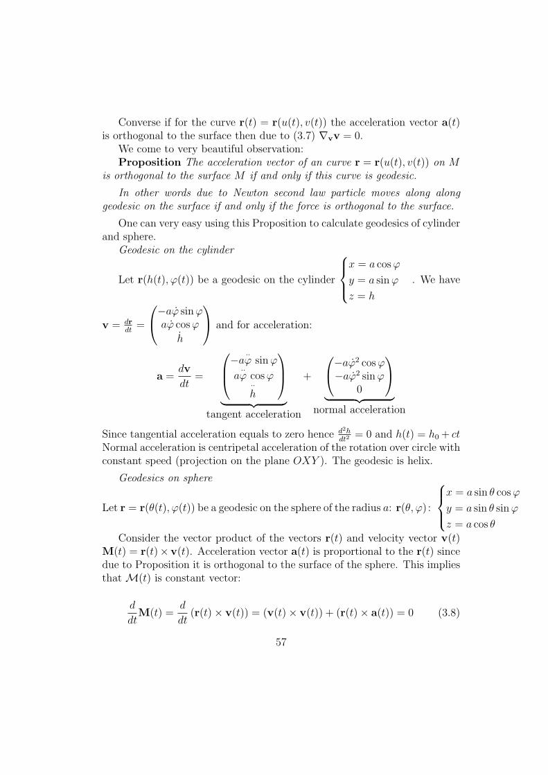
Converse if for the curve r(t) = r(u(t), v(t)) the acceleration vector a(t)is orthogonal to the surface then due to (3.7) ∇vv = 0.

We come to very beautiful observation:Proposition The acceleration vector of an curve r = r(u(t), v(t)) on M

is orthogonal to the surface M if and only if this curve is geodesic.

In other words due to Newton second law particle moves along alonggeodesic on the surface if and only if the force is orthogonal to the surface.

One can very easy using this Proposition to calculate geodesics of cylinderand sphere.

Geodesic on the cylinder

Let r(h(t), φ(t)) be a geodesic on the cylinder

x = a cosφ

y = a sinφ

z = h

. We have

v = drdt

=

−aφ sinφaφ cosφ

h

and for acceleration:

a =dv

dt=

−a··φ sinφ

a··φ cosφ

··h

︸︷︷︸

tangent acceleration

+

−aφ2 cosφ−aφ2 sinφ

0

︸︷︷︸

normal acceleration

Since tangential acceleration equals to zero hence d2hdt2

= 0 and h(t) = h0 + ctNormal acceleration is centripetal acceleration of the rotation over circle withconstant speed (projection on the plane OXY ). The geodesic is helix.

Geodesics on sphere

Let r = r(θ(t), φ(t)) be a geodesic on the sphere of the radius a: r(θ, φ) :

x = a sin θ cosφ

y = a sin θ sinφ

z = a cos θ

Consider the vector product of the vectors r(t) and velocity vector v(t)M(t) = r(t)× v(t). Acceleration vector a(t) is proportional to the r(t) sincedue to Proposition it is orthogonal to the surface of the sphere. This impliesthat M(t) is constant vector:

d

dtM(t) =

d

dt(r(t)× v(t)) = (v(t)× v(t)) + (r(t)× a(t)) = 0 (3.8)

57

We have M(t) = M0. r(t) is orthogonal to M = r(t) × v(t). We seethat r(t) belongs to the sphere and to the plane orthogonal to the vectorM0 = r(t) × v(t). The intersection of this plane with sphere is a greatcircle. We proved that if r(t) is geodesic hence it belongs to great circle (asun-parameterised curve).

The converse is evident since if particle moves along the great circle withconstant velocity then obviously acceleration vector is orthogonal to the sur-face.

Remark The vector M = r(t) × v(t) is the torque. The torque is inte-gral of motion in isotropic space.—This is the core of the considerations forgeodesics on the sphere.

3.3 Geodesics and Lagrangians of ”free” particle onRiemannian manifold.

3.3.1 Lagrangian and Euler-Lagrange equations

A function L = L(x, x) on points and velocity vectors on manifold M is aLagrangian on manifold M .

We assign to Lagrangian L = L(x, x) the following second order differen-tial equations

d

dt

(∂L

∂xi

)=

∂L

∂xi(3.9)

In detaild

dt

(∂L

∂xi

)=

∂2L

∂xm∂xixm +

∂2L

∂xm∂xi

··xm=

∂L

∂xi. (3.10)

These equations are called Euler-Lagrange equations of the LagrangianL. We will explain later the variational origin of these equations 8.

3.3.2 Lagrangian of ”free” particle

Let (M,G), G = gikdxidxk be a Riemannian manifold.

8To every mechanical system one can put in correspondence a Lagrangian on config-uration space. The dynamics of the system is described by Euler-Lagrange equations.The advantage of Lagrangian approach is that it works in an arbitrary coordinate system:Euler-Lagrange equations are invariant with respect to changing of coordinates since theyarise from variational principe.

58

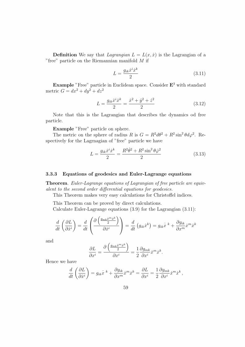
Definition We say that Lagrangian L = L(x, x) is the Lagrangian of a”free” particle on the Riemannian manifold M if

L =gikx

ixk

2(3.11)

Example ”Free” particle in Euclidean space. Consider E3 with standardmetric G = dx2 + dy2 + dz2

L =gikx

ixk

2=

x2 + y2 + z2

2(3.12)

Note that this is the Lagrangian that describes the dynamics od freeparticle.

Example ”Free” particle on sphere.The metric on the sphere of radius R is G = R2dθ2 + R2 sin2 θdφ2. Re-

spectively for the Lagrnagian of ”free” particle we have

L =gikx

ixk

2=

R2θ2 +R2 sin2 θφ2

2(3.13)

3.3.3 Equations of geodesics and Euler-Lagrange equations

Theorem. Euler-Lagrange equations of Lagrangian of free particle are equiv-alent to the second order differential equations for geodesics.

This Theorem makes very easy calculations for Christoffel indices.

This Theorem can be proved by direct calculations.Calculate Euler-Lagrange equations (3.9) for the Lagrangian (3.11):

d

dt

(∂L

∂xi

)=

d

dt

∂(

gmkxmxk

2

)∂xi

=d

dt

(gikx

k)= gik

··x k +

∂gik∂xm

xmxk

and

∂L

∂xi=

∂(

gmkxmxk

2

)∂xi

=1

2

∂gmk

∂xixmxk.

Hence we have

d

dt

(∂L

∂xi

)= gik

··x k +

∂gik∂xm

xmxk =∂L

∂xi=

1

2

∂gmk

∂xixmxk ,

59

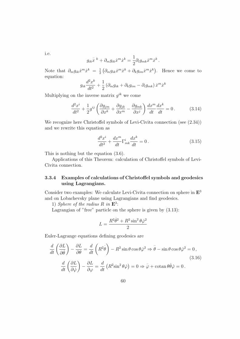
i.e.

gik··x k + ∂mgikx

mxk =1

2∂igmkx

mxk .

Note that ∂mgikxmxk = 1

2

(∂mgikx

mxk + ∂kgimxmxk

). Hence we come to

equation:

gikd2xk

dt2+

1

2(∂mgik + ∂kgim − ∂igmk) x

mxk

Multiplying on the inverse matrix gik we come

d2xi

dt2+

1

2gij(∂gjm∂xk

+∂gjk∂xm

− ∂gmk

∂xj

)dxm

dt

dxk

dt= 0 . (3.14)

We recognize here Christoffel symbols of Levi-Civita connection (see (2.34))and we rewrite this equation as

d2xi

dt2+

dxm

dtΓimk

dxk

dt= 0 . (3.15)

This is nothing but the equation (3.6).Applications of this Theorem: calculation of Christoffel symbols of Levi-

Civita connection.

3.3.4 Examples of calculations of Christoffel symbols and geodesicsusing Lagrangians.

Consider two examples: We calculate Levi-Civita connection on sphere in E3

and on Lobachevsky plane using Lagrangians and find geodesics.1) Sphere of the radius R in E3:Lagrangian of ”free” particle on the sphere is given by (3.13):

L =R2θ2 +R2 sin2 θφ2

2

Euler-Lagrange equations defining geodesics are

d

dt

(∂L

∂θ

)− ∂L

∂θ=

d

dt

(R2

·θ

)−R2 sin θ cos θφ2 ⇒

··θ − sin θ cos θφ2 = 0 ,

(3.16)d

dt

(∂L

∂φ

)− ∂L

∂φ=

d

dt

(R2sin2 θφ

)= 0 ⇒ ··

φ+ cotan θθφ = 0 .

60

Comparing Euler-Lagrange equations with equations for geodesic in terms ofChristoffel symbols:

··θ + Γθ

θθθ2 + 2Γθ

θφθφ+ Γθφφφ

2 = 0,

··φ+ Γφ

θθθ2 + 2Γφ

θφθφ+ Γφφφφ

2 = 0

we come toΓθθθ = Γθ

θφ = Γθφθ = 0 ,Γθ

φφ = − sin θ cos θ , (3.17)

Γφθθ = Γφ

φφ = 0, Γφθφ = Γφ

φθ = cotan θ . (3.18)

(Compare with previous calculations for connection in subsections 2.2.1 and2.3.4)

We proved that geodesics on the sphere are great circles. (see subsection 3.2.3 above).Consider another more straightforward proof of this fact. To find geodesics one have tosolve second order differential equations (3.16):

One can see that the great circles: φ = φ0, θ = θ0 + t are solutions of second orderdifferential equations (3.16) with initial conditions

θ(t)∣∣t=0

= θ0, θ(t)∣∣t=0

= 1, φ(t)∣∣t=0

= φ0, θ(t)∣∣t=0

= 0 . (3.19)

The rotation of the sphere is isometry, which does not change Levi-Civta connection.Hence an arbitrary great circle is geodesic.

Prove that an arbitrary geodesic is an arc of great circle. Let the curve θ = θ(t), φ =φ(t), 0 ≤ t ≤ t1 be geodesic. Rotating the sphere we can come to the curve θ = θ′(t), φ =φ′(t), 0 ≤ t ≤ t1 such that velocity vector at the initial time is direccted along meridian,i.e. initial conditions are

θ′(t)∣∣t=0

= θ0, θ′(t)∣∣t=0

= a, φ′(t)∣∣t=0

= φ0, φ′(t)∣∣t=0

= 0 . (3.20)

(Compare with initial conditions (3.19)) Second order differential equations with boundaryconditions for coordinates and velocities at t = 0 have unique solution. The solutions ofsecond order differential equations (3.16) with initial conditions (3.20) is a curve θ′(t) =θ0 + at, φ′(t) = φ0. It is great circle. Hence initial curve the geodesic θ = θ(t), φ = φ(t),0 ≤ t ≤ t1 is an arc of great circle too.

This is another proof that geodesics are great circles.

2) Lobachevsky plane.Lagrangian of ”free” particle on the Lobachevsky plane with metric G =

dx2+dy2

y2is

L =1

2

x2 + y2

y2.

Euler-Lagrange equations are

61

∂L

∂x= 0 =

d

dt

∂L

∂x=

d

dt

(x

y2

)=

··x

y2− 2xy

y3, i.e.

··x− 2xy

y= 0 ,

∂L

∂y= − x2 + y2

y3=

d

dt

∂L

∂y=

d

dt

(y

y2

)=

··y

y2− 2y2

y3, i.e.

··y +

x2

y− y2

y= 0 .

Comparing these equations with equations for geodesics:··xi− xkΓi

kmxm = 0

(i = 1, 2, x = x1, y = x2) we come to

Γxxx = 0,Γx

xy = Γxyx = −1

y, Γx

yy = 0, Γyxx =

1

y,Γy

xy = Γyyx = 0,Γy

yy = −1

y.

In a similar way as for a sphere one can find geodesics on Lobachevsky plane. First we

note that vertical rays are geodesics. Then using the inversions with centre on the absolute

one can see that arcs of the circles with centre at the absolute (y = 0) are geodesics too.

3.3.5 Variational principe and Euler-Lagrange equations

Here very briefly we will explain how Euler-Lagrange equations follow fromvariational principe.

Let M be a manifold (not necessarily Riemannian) and L = L(xi, xi) bea Lagrangian on it.

Denote my Mx2,t2

x1,t1the space of curves (paths) such that they start at the

point x1 at the ”time” t = t1 and end at the point x2 at the ”time” t = t2:

Mx2,t2

x1,t1= {C : x(t), t1 ≤ t ≤ t2, x(t1) = x1,x(t2) = x2} . (3.21)

Consider the following functional S on the space Mx2,t2

x1,t1:

S [x(t)] =

∫ t2

t1

L(xi(t), xi(t)

)dt . (3.22)

for every curve x(t) ∈ Mx2,t2

x1,t1.

This functional is called action functional.Theorem Let functional S attaints the minimal value on the path x0(t) ∈

Mx2,t2

x1,t1, i.e.

∀x(t) ∈ Mx2,t2

x1,t1S[x0(t)] ≤ S[x(t)] . (3.23)

62

Then the path x0(t) is a solution of Euler-Lagrange equations of the La-grangian L:

d

dt

(∂L

∂xi

)=

∂L

∂xiif x(t) = x0(t) . (3.24)

Remark The path x(t) sometimes is called extremal of the action func-tional (3.22).

We will use this Theorem to show that the geodesics are in some senseshortest curves 9.

3.4 Geodesics and shortest distance.

Many of you know that geodesics are in some sense shortest curves. Wewill give an exact meaning to this statement and prove it using variationalprincipe:

Let M be a Riemannian manifold.Theorem Let x1 and x2 be two points on M . The shortest curve which

joins these points is an arc of geodesic.Let C be a geodesic on M and x1 ∈ C. Then for an arbitrary point x2 ∈ C

which is close to the point x1 the arc of geodesic joining the points x1,x2 isa shortest curve between these points10 .

This Theorem makes a bridge between two different approach to geodesic:the shortest disntance and parallel transport of velocity vector.

Sketch a proof:Consider the following two Lagrangians: Lagrangian of a ”free ” particle

Lfree =gik(x)x

ixk

2and the length Lagrangian

Llength(x, x) =√gik(x)xixk =

√2Lfree .

9The statement of this Theorem is enough for our purposes. In fact in classical mechan-ics another more useful statement is used: the path x0(t) is a solution of Euler-Lagrangeequations of the Lagrangian L if and only if it is the stationary ”point” of the actionfunctional (3.22), i.e.

S[x0(t) + δx(t)]− S[x0(t) + δx(t)] = 0(δx(t)) (3.25)

for an arbitrary infinitesimal variation of the path x0(t): δx(t1) = δx(t2) = 0.10More precisely: for every point x1 ∈ C there exists a ball Bδ(x1) such that for an

arbitrary point x2 ∈ C ∩Bδ(x1) the arc of geodesic joining the points x1,x2 is a shortestcurve between these points.

63

If C : xi(t), t1 ≤ t ≤ t2 is a curve on M then

Length of the curve C =∫ t2

t1

Llength(xi(t), xi(t))dt =

∫ t2

t1

√gik(x(t))xi(t)xk(t)dt . (3.26)

The proof of the Theorem follows from the following observation:Observation Euler-Lagrange equations for the length functional (3.26) are

equivalent to the Euler-Lagrange equations for action functional (3.22). Thismeans that extremals of the length functional and action functionals coincide.

Indeed it follows from this observation and the variational principe thatthe shortest curves obey the Euler-Lagrange equations for the action func-tional. We showed before that Euler-Lagrange equations for action functional(3.22) define geodesics. Hence the shortest curves are geodesics.

One can check the observation by direct calculation: Calculate Euler-Lagrange equations for the Lagrangian Llength =

√gik(x)xixk =

√2Lfree:

d

dt

(∂Llength

∂xi

)− ∂Llength

∂xi=

d

dt

(1√

gikxixkgikx

k

)− 1

2√

gikxixk

∂gkmxkxm

∂xi

=d

dt

(1

Llength

∂Lfree

∂xi

)− 1

Llength

∂Lfree

∂xi= 0 . (3.27)

To facilitate calculations note that the length functional (3.26) is repa-rameterisation invariant. Choose the natural parameter s(t) or a parame-ter proportional to the natural parameter on the curve xi(t). We come toLlength = const and it follows from (3.27) that

d

dt

(∂Llength

∂xi

)− ∂Llength

∂xi=

1

Llength

(d

dt

(∂Lfree

∂xi

)− ∂Lfree

∂xi

)= 0 .

We prove that Euler-Lagrange equations for length and action Lagrangianscoincide.

In the Euclidean space straight lines are the shortest distances betweentwo points. On the other hand their velocity vectors are constant. We realisenow that in general Riemannian manifold the role of geodesic is twofold also:they are locally shortest and have covariantly constant velocity vectors.

64

3.4.1 Again geodesics for sphere and Lobachevsky plane

The fact that geodesics are shortest gives us another tool to calculate geodesics.Consider again examples of sphere and Lobachevsky plane and find geodesics

using the fact that they are shortest. The fact that geodesics are locally theshortest curves

Consider again sphere in E3 with the radius R: Coordinates θ, φ, inducedRiemannian metrics (first quadratic form):

G = R2(dθ2 + sin2 θdφ2) . (3.28)

Consider two arbitrary points A and B on the sphere. Let (θ0, φ0) be coor-dinates of the point A and (θ1, φ1) be coordinates of the point B

Let CAB be a curve which connects these points: CAB : θ(t), φ(t) suchthat θ(t0) = θ0, θ(t1) = θ1, φ(t0) = θ0, θ(t1) = θ1 then:

LCAB=

∫R√θ2t + sin2 θ(t)φ2

tdt (3.29)

Suppose that points A and B have the same latitude, i.e. if (θ0, φ0) arecoordinates of the point A and (θ1, φ1) are coordinates of the point B thenφ0 = φ1 (if it is not the fact then we can come to this condition rotating thesphere)

Now it is easy to see that an arc of meridian, the curve φ = φ0 is geodesics:Indeed consider an arbitrary curve θ(t), φ(t) which connects the points A,B:θ(t0) = θ(t1) = θ0, φ(t0) = φ(t1) = φ0. Compare its length with the lengthof the meridian which connects the points A, B:∫ t1

t0

R

√θ2t + sin2 θφ2

tdt ≥ R

∫ t1

t0

√θ2t dt = R

∫ t1

t0

θtdt = R(θ1 − θ0) (3.30)

Thus we see that the great circle joining points A,B is the shortest. Thegreat circles on sphere are geodesics. It corresponds to geometrical intuition:The geodesics on the sphere are the circles of intersection of the sphere withthe plane which crosses the centre.

Geodesics on Lobachevsky planeRiemannian metric on Lobachevsky plane:

G =dx2 + dy2

y2(3.31)

65

The length of the curve γ : x = x(t, y = y(t)) is equal to

L =

∫ √x2t + y2ty2(t)

dt

In particularly the length of the vertical interval [1, ε] tends to infinity ifε → 0:

L =

∫ √x2t + y2ty2(t)

dt =

∫ 1

ε

√1

t2dt = log

1

ε

One can see that the distance from every point to the line y = 0 is equal toinfinity. This motivates the fact that the line y = 0 is called absolute.

Consider two points A = (x0, y0), B = (x1, y1) on Lobachevsky plane.It is easy to see that vertical lines are geodesics of Lobachevsky plane.Namely let points A,B are on the ray x = x0. Let CAB be an arc of

the ray x = x0 which joins these points: CAB : x = x0, y = y0 + t Thenit is easy to see that the length of the curve CAB is less or equal than thelength of the arbitrary curve x = x(t), y = y(t) which joins these points:x(t)

∣∣t=0

= x0, y(t)∣∣t=0

= y0, x(t)∣∣t=t1

= x0, y(t)∣∣t=t1

= y1:

∫ t

0

√x2t + y2ty2(t)

dt ≥∫ t

0

√y2t

y2(t)dt =

∫ y1

y0

dt

tdt = log

y1y0

= length of CAB

Hence CAB is shortest. We prove that vertical rays are geodesics.Consider now the case if x0 = x1. Find geodesics which connects two

points A,B which are not on the same vertical ray. Consider semicirclewhich passes these two points such that its centre is on the absolute. Weprove that it is a geodesic.

Proof Let coordinates of the centre of the circle are (a, 0). Then consider polar coor-dinates (r, φ):

x = a+ r cosφ, y = r sinφ (3.32)

In these polar coordinates r-coordinate of the semicircle is constant.Find Lobachevsky metric in these coordinates: dx = −r sinφdφ + cosφdr, dy =

r cosφdφ+ sinφdr, dx2 + dy2 = dr2 + r2dφ2. Hence:

G =dx2 + dy2

y2=

dr2 + r2dφ2

r2 sin2 φ==

dφ2

sin2 φ+

dr2

r2 sin2 φ(3.33)

66

We see that the length of the arbitrary curve which connects points A,B is greater orequal to the length of the arc of the circle:

LAB =

∫ t1

t0

√φ2t

sin2 φ+

r2tr2 sin2 φ

dt ≥∫ t1

t0

√φ2t

sin2 φdt = (3.34)

∫ t1

t0

φt

sinφdt =

∫ φ1

φ0

dφ

sinφ= log

tanφ1

tanφ1

The proof is finished.

4 Surfaces in E3

Now equipped by the knowledge of Riemannian geometry we consider sur-faces in E3. We reconsider again conceptions of Shape (Weingarten) opera-tor, Gaussian and mean curvatures, focusing attention on the the fact whatproperties are internal and what properties are external.

4.1 Formulation of the main result. Theorem of paral-lel transport over closed curve and Theorema Egregium

Let M be a surface in Euclidean space E3. Consider a closed curve C on M ,M : r = r(u, v), C : r = r(u(t, v(t)), 0 ≤ t ≤ t1, x(0) = x(t1). (u(t), v(t) areinternal coordinates of the curve C.)

Consider the parallel transport of an arbitrary tangent X vector alongthe closed curve C:

X(t) = Xα(t)∂

∂uα

∣∣uα(t)︸︷︷︸

Internal observer

= Xα(t)rα∣∣r(u(t),v(t))︸︷︷︸

External observer

,

(rα =

∂xi

∂uα

∂

∂xi

).

X(t) :∇X(t)

dt= 0, 0 ≤ t ≤ t1 ,

i.e.dXα(t)

dt+Xβ(t)Γα

βγ(u(t))duγ(t)

dt= 0, 0 ≤ t ≤ t1 , (4.1)

where ∇ is the connection induced on the surface M by canonical flat con-nection (see (??)), i.e. the Levi-Civita connection of the induced Riemannian

67

metric on the surface M and Γαβγ its Christoffel symbols:

Γγαβ =

1

2gγπ(∂gπα∂uβ

+∂gπβ∂uα

− ∂gαβ∂uπ

),where gαβ = ⟨rα, rβ⟩ =

∂xi

∂uα

∂xi

∂uβ

(4.2)are components of induced Riemannian metric GM = gαβdu

αduβ/Let r(0) = p be a starting (and ending) point of the curve C: r(0) =

r(t1) = p. The differential equation (4.1) defines the linear operator

RC : TpM −→ TpM (4.3)

For any vector X ∈ TpM , its image the vector RCX as the solution of thedifferential equation (4.1) with initial condition X(t)

∣∣t=0

= X.On the other hand we know that parallel transport of the vector does not

change its length (see (3.5) in the subsection 3.2.1):

⟨X,X⟩ = ⟨RCX, RCX⟩ (4.4)

We see that RC is an orthogonal operator in the 2-dimensional vector spaceTpM . We know that orthogonal operator preserving orientation is the oper-ator of rotation on some angle Φ.

We see that if RC preserves orientation11 then the action of operator RC

on vectors is rotation on the angle, i.e. the result of parallel transport alongclosed curve is rotation on the angle

∆Φ = ∆Φ(C) (4.5)

which depends on the curve.The very beautiful question arises: How to calculate this angle ∆Φ(C)

Theorem Let M be a surface in Euclidean space E3. Let C be a closedcurve C on M such that C is a boundary of a compact oriented domainD ⊂ M . Consider the parallel transport of an arbitrary tangent vector alongthe closed curve C. As a result of parallel transport along this closed curveany tangent vector rotates through the angle

∆Φ = ∠ (X,RCX) =

∫D

Kdσ , (4.6)

11We consider the case if the operator RC preserves orientation. In our considerationswe consider only the case if the closed curve C is a boundary of a compact oriented domainD ⊂ M . In this case one can see that operator RC preserves an orientation.

68

where K is the Gaussian curvature and dσ =√det gdudv is the area element

induced by the Riemannian metric on the surface M , i.e. dσ =√det gdudv.

Remark One can show that the angle of rotation does not depend oninitial point of the curve.

Example Consider the closed curve, ”latitude” Cθ0 : θ = θ0 on the sphereof the radius R. Calculations show that

∆Φ(Cθ0) = 2π(1− cos θ0) (4.7)

(see the Homework 6). On the other hand the latitude Cθ0 is the boundaryof the segment D with area 2πRH where H = R(1− cos θ0). Hence

∠ (X,RCX) =2πRH

R2=

1

R2· area of the segment =

∫D

Kdσ

since Gaussian curvature is equal to 1R2

The proof of this Theorem is the content of the subsections above.

4.1.1 GaußTheorema Egregium

Show that this Theorem implies the remarkable corollary.Let D be a small domain around a given point p, let C its boundary

and ∆Φ(D) the angle of rotation. Denote by S(D) an area of this domain.Applying the Theorem for the case when area of the domain D tends to zerowe we come to the statement that

if S(D) → 0 then ∆Φ(D) =

∫D

Kdσ → K(p)S(D), i.e.

K(p) = limS(D)→0

∆Φ(D)

S(D), i.e. (4.8)

Now notice that left hand side od this equation defining Gaussian cur-vature K(p) depends only on Riemannian metric on the surface C. Indeednumerator of LHS is defined by the solution of differential equation (4.1)which depends on Levi-Civita connection depending on the induced Rieman-nian metric, and denominator is an area depending on Riemannian metrictoo.

Thus we come to very important

69

Corollary Gauß Egregium TheoremaGaussian curvature of the surface is invariant of isometries.

In next subsections we develop the technique which itself is very interest-ing. One of the applications of this technique is the proof of the Theorem(4.6). Thus we will prove Theorema Egregium too.

Later in the fifth section we will give another proof of the TheoremaEgregium.

4.2 Derivation formulae

Let M be a surface embedded in Euclidean space E3, M : r = r(u, v).Let e, f ,n be three vector fields defined on the points of this surface such

that they form an orthonormal basis at any point, so that the vectors e, fare tangent to the surface and the vector n is orthogonal to the surface12.Vector fields e, f ,n are functions on the surface M :

e = e(u, v), f = f(u, v) ,n = n(u, v) .

Consider 1-forms de, df , dn:

de =∂e

∂udu+

∂e

∂vdv, df =

∂f

∂udu+

∂f

∂vdv , dn =

∂n

∂udu+

∂n

∂vdv

These 1-forms take values in the vectors in E3, i.e. they are vector valued1-forms. Any vector in E3 attached at an arbitrary point of the surface canbe expanded over the basis {e, f ,n}. Thus vector valued 1-forms de, df , dncan be expanded in a sum of 1-forms with values in basic vectors e, f ,n. E.g.for de = ∂e

∂udu+ ∂e

∂vdv expanding vectors ∂e

∂uand ∂e

∂vover basis vectors we come

to

∂e

∂u= A1(u, v)e+B1(u, v)f+C1(u, v)n,

∂e

∂v= A2(u, v)e+B2(u, v)f+C2(u, v)n

thus

de =∂e

∂udu+

∂e

∂vdv = (A1e+B1f + C1n) du+ (A2e+B2f + C2n) dv =

12One can say that {e, f ,n} is an orthonormal basis in TpE3 at every point of surface

p ∈ M such that {e, f} is an orthonormal basis in TpE3 at every point of surface p ∈ M .

70

= (A1du+ A2dv)︸︷︷︸M11

e+ (B1du+B2dv)︸︷︷︸M12

f + (C1du+ C2dv)︸︷︷︸M11

e, (4.9)

i.e.de = M11e+M12f +M13n,

where M11,M12 and M13 are 1-forms on the surface M defined by the relation(4.9).

In the same way we do the expansions of vector-valued 1-forms df anddn we come to

de = M11e+M12f +M13ndf = M21e+M22f +M23ndn = M31e+M32f +M33n

This equation can be rewritten in the following way:

d

efn

=

M11 M12 M13

M21 M22 M23

M31 M32 M33

efn

(4.10)

Proposition The matrix M in the equation (4.10) is antisymmetrical ma-trix, i.e.

M11 = M22 = M33 = 0M12 = −M21 = aM13 = −M31 = bM23 = −M32 = −b

(4.11)

i.e.

d

efn

=

0 a b−a 0 c−b −c 0

efn

, (4.12)

where a, b, c are 1-forms on the surface M .

Formulae (5.13) are called derivation formulae.Prove this Proposition. Recall that {e, f ,n} is orthonormal basis, i.e. at

every point of the surface

⟨e, e⟩ = ⟨f , f⟩ = ⟨n,n⟩ = 1, and ⟨e, f⟩ = ⟨e,n⟩ = ⟨f ,n⟩ = 0

Now using (4.10) we have

⟨e, e⟩ = 1 ⇒ d⟨e, e⟩ = 0 = 2⟨e, de⟩ = ⟨e,M11e+M12f +M13n⟩ =

71

M11⟨e, e⟩+M12⟨e, f⟩+M13⟨e,n⟩ = M11 ⇒ M11 = 0 .

Analogously

⟨f , f⟩ = 1 ⇒ d⟨f , f⟩ = 0 = 2⟨f , df⟩ = ⟨f ,M21e+M22f+M23n⟩ = M22 ⇒ M22 = 0 ,

⟨n,n⟩ = 1 ⇒ d⟨n,n⟩ = 0 = 2⟨n, dn⟩ = ⟨n,M31e+M32f+M33n⟩ = M33. ⇒ M33 = 0 .

We proved already that M11 = M22 = M33 = 0. Now prove that M12 =−M21, M13 = −M31 and M13 = −M31.

⟨e, f⟩ = 0 ⇒ d⟨e, f⟩ = 0 = ⟨e, df⟩+ ⟨de, f⟩ =

⟨e,M21e+M22f +M23n⟩+ ⟨M11e+M12f +M13n, f⟩ = M21 +M12 = 0.

Analogously

⟨e,n⟩ = 0 ⇒ d⟨e,n⟩ = 0 = ⟨e, dn⟩+ ⟨de,n⟩ =

⟨e,M31e+M32f +M33n⟩+ ⟨M11e+M12f +M13n,n⟩ = M31 +M13 = 0

and⟨f ,n⟩ = 0 ⇒ d⟨f ,n⟩ = 0 = ⟨f , dn⟩+ ⟨df ,n⟩ =

⟨f ,M31e+M32f +M33n⟩+ ⟨M21e+M22f +M23n,n⟩ = M32 +M23 = 0.

Remark This proof could be performed much more shortly in condensednotations. Derivation formulae (5.13) in condensed notations are

dei = Mikek (4.13)

Orthonormality condition means that ⟨ei, ek⟩ = δik. Hence

d⟨ei, ek⟩ = 0 = ⟨dei, ek⟩+⟨ei, dek⟩ = ⟨Mimem, ek⟩+⟨ei,Mknen⟩ = Mik+Mki = 0

(4.14)Much shorter, is not it?

4.2.1 ∗Gauss condition (structure equations)

Derive the relations between 1-forms a, b and c in derivation formulae.Recall that a, b, c are 1-forms, e, f,n are vector valued functions (0-forms)

and de, df , dn are vector valued 1-forms. (We use the simple identity that

72

ddf = 0 and the fact that for 1-form ω ∧ ω = 0.) We have from derivationformulae (5.13) that

d2e = 0 = d(af + bn) = daf − a ∧ df + dbn− b ∧ dn =

da f − a ∧ (−ae+ cn) + dbn− b ∧ (−be− cf) =

(da+b∧c)f+(a∧a+b∧b)e+(db−a∧c)n = (da+b∧c)f+(db+c∧a)n = 0 .

We see that(da+ b ∧ c)f + (db+ c ∧ a)n = 0 (4.15)

Hence components of the left hand side equal to zero:

(da+ b ∧ c) = 0 (db+ c ∧ a) = 0 . (4.16)

Analogously

d2f = 0 = d(−ae+ cn) = −dae+ a ∧ de+ dcn− c ∧ dn =

−dae+ a ∧ (af + bn) + dcn− c ∧ (−be− cf) =

(−da+ c ∧ b)e+ (dc+ a ∧ b)n = 0 .

Hence we come to structure equations:

da+ b ∧ c = 0db+ c ∧ a = 0dc+ a ∧ a = 0

(4.17)

4.3 Geometrical meaning of derivation formulae. Wein-garten operator and second quadratic form in termsof derivation formulae.

Let M be a surface in E3.Let e, f ,n be three vector fields defined on the points of this surface such

that they form an orthonormal basis at any point, so that the vectors e, f aretangent to the surface and the vector n is orthogonal to the surface. Notethat in generally these vectors are not coordinate vectors.

Describe Riemannian geometry on the surface M in terms of this basisand derivation formulae (5.13).

Induced Riemannian metric

73

If G is the Riemannian metric induced on the surface M then since e, fis orthonormal basis at every tangent space TpM then

G(e, e) = G(f , f) = 1, G(e, f) = G(f , e) = 0 (4.18)

The matrix of the Riemannian metric in the basis {e, f} is

G =

(1 00 1

)(4.19)

Induced connection Let ∇ be the connection induced by the canonical flatconnection on the surface M .

Then according equations (??) and derivation formulae (5.13) for everytangent vector X

∇Xe = (∂Xe)tangent = (de(X))tangent = (a(X)f + b(X)n)tangent = a(X)f .(4.20)

and

∇Xf = (∂Xf)tangent = (df(X))tangent = (−a(X)e+ c(X)n)tangent = −a(X)e .(4.21)

In particular∇ee = a(e)f ∇fe = a(f)f∇ef = −a(e)e ∇f f = −a(f)e

(4.22)

We know that the connection ∇ is Levi-Civita connection of the inducedRiemannian metric (4.20) (see the subsection 4.2.1)13.

Second Quadratic form Second quadratic form is a bilinear symmetric functionA(X,Y)on tangent vectors which is well-defined by the condition A(X,Y)n = (∂XY)orthogonal (seee.g. subsection 6.4 in Appendices.)

Let A(X,Y) be second quadratic form. Then according to derivation formulae (5.13)we have

A(e, e) = ⟨∂ee,n⟩ = ⟨de(e),n⟩ = ⟨a(e)f + b(e)n,n⟩ = b(e) ,

A(f , e) = ⟨∂fe,n⟩ = ⟨de(f),n⟩ = ⟨a(f)f + b(f)n,n⟩ = b(f) ,

A(e, f) = ⟨∂ef ,n⟩ = ⟨df(e),n⟩ = ⟨−a(e)f + c(e)n,n⟩ = c(e) ,

13In particular this implies that this is symmetric connection, i.e.

∇fe−∇ef − [f , e] = a(f)f + a(e)e− [f , e] = 0 . (4.23)

74

A(f , f) = ⟨∂f f ,n⟩ = ⟨df(f),n⟩ = ⟨−a(f)f + c(f)n,n⟩ = c(f) ,

The matrix of the second quadratic form in the basis {e, f} is

A =

(A(e, e) A(f , e)A(e, f) A(f , f)

)=

(b(e) b(f)c(e) c(f)

)(4.24)

This is symmetrical matrix (see the subsection 4.3.2):

A(f , e) = b(f) = A(e, f) = c(e) . (4.25)

Weingarten operatorLet S be Weingarten operator: SX = −∂Xn (see the subsection 6.4 in

Appendix, or last year Geometry letures). Then it follows from derivationformulae that

SX = −∂Xn = −dn(X) = − (−b(X)e− c(X)f) = b(X)e+ c(X)f

In particular

S(e) = b(e)e+ c(e)f , S(f) = b(f)e+ c(f)f

and the matrix of the Weingarten operator in the basis {e, f} is

S =

(b(e) c(e)b(f) c(f)

)(4.26)

Remark According to the condition (4.25) the matrix S is symmetrical. The relations

A = GS, S = G−1A for Weingarten operator, Riemannian metric and second quadratic

form are evidently obeyed for matrices of these operators in the basis e, f where G = 1,

A = S.

4.3.1 Gaussian and mean curvature in terms of derivation formu-lae

Now we are equipped to express Gaussian and mean curvatures in terms ofderivation formulae. Using (4.26) we have for Gaussian curvature

K = detS = b(e)c(f)− c(e)b(f) = (b ∧ c)(e, f) (4.27)

and for mean curvature

H = TrS = b(e) + c(f) (4.28)

What next? We will study in more detail formula (4.27) later.Now consider some examples of calculation derivation formulae, Wein-

garten operator, e.t..c. for some examples using derivation formulae.

75

4.4 Examples of calculations of derivation formulae andcurvatures for cylinder, cone and sphere

Last year we calculated Weingarten oeprator, second quadratic form andcurvatures for cylinder, cone and sphere (see also the subsection 6.4 in Ap-pendices.). Now we do the same but in terms of derivation formulae.

Cylinder

We have to define three vector fields e, f ,n on the points of the cylinder

r(h, φ) :

x = R cosφ

y = R sinφ

z = h

such that they form an orthonormal basis at any

point, so that the vectors e, f are tangent to the surface and the vector n isorthogonal to the surface. We calculated many times coordinate vector fieldsrh, rφ and normal unit vector field:

rh =

001

, rφ =

−R sinφR cosφ

0

, n =

cosφsinφ0

. (4.29)

Vectors rh, rφ and n are orthogonal to each other but not all of them haveunit length. One can choose

e = rh =

001

, f =rφR

=

− sinφcosφ0

, n =

cosφsinφ0

(4.30)

These vectors form an orthonormal basis and e, f form an orthonormal basisin tangent space.

Derive for this basis derivation formulae (5.13). For vector fields e, f ,nin (4.30) we have

de = 0, df = d

− sinφcosφ0

=

− cosφ− sinφ

0

dφ = −ndφ,

dn = d

cosφsinφ0

=

− sinφcosφ0

= fdφ,

76

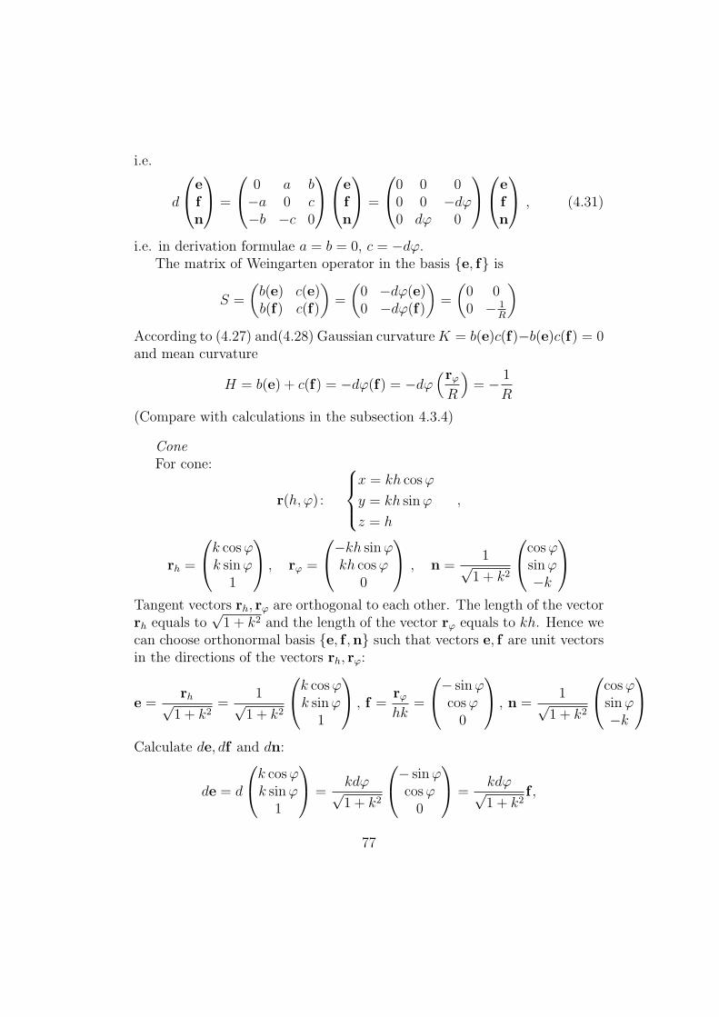
i.e.

d

efn

=

0 a b−a 0 c−b −c 0

efn

=

0 0 00 0 −dφ0 dφ 0

efn

, (4.31)

i.e. in derivation formulae a = b = 0, c = −dφ.The matrix of Weingarten operator in the basis {e, f} is

S =

(b(e) c(e)b(f) c(f)

)=

(0 −dφ(e)0 −dφ(f)

)=

(0 00 − 1

R

)According to (4.27) and(4.28) Gaussian curvatureK = b(e)c(f)−b(e)c(f) = 0and mean curvature

H = b(e) + c(f) = −dφ(f) = −dφ(rφR

)= − 1

R

(Compare with calculations in the subsection 4.3.4)

ConeFor cone:

r(h, φ) :

x = kh cosφ

y = kh sinφ

z = h

,

rh =

k cosφk sinφ

1

, rφ =

−kh sinφkh cosφ

0

, n =1√

1 + k2

cosφsinφ−k

Tangent vectors rh, rφ are orthogonal to each other. The length of the vectorrh equals to

√1 + k2 and the length of the vector rφ equals to kh. Hence we

can choose orthonormal basis {e, f ,n} such that vectors e, f are unit vectorsin the directions of the vectors rh, rφ:

e =rh√1 + k2

=1√

1 + k2

k cosφk sinφ

1

, f =rφhk

=

− sinφcosφ0

, n =1√

1 + k2

cosφsinφ−k

Calculate de, df and dn:

de = d

k cosφk sinφ

1

=kdφ√1 + k2

− sinφcosφ0

=kdφ√1 + k2

f ,

77

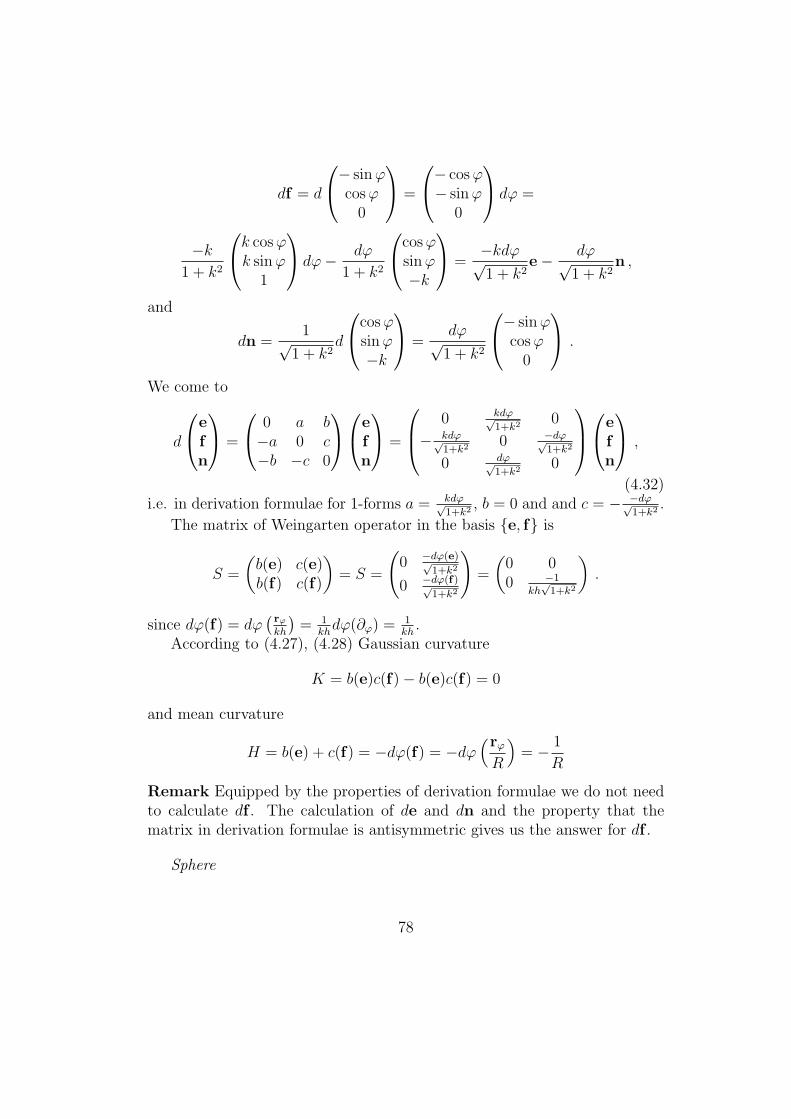
df = d

− sinφcosφ0

=

− cosφ− sinφ

0

dφ =

−k

1 + k2

k cosφk sinφ

1

dφ− dφ

1 + k2

cosφsinφ−k

=−kdφ√1 + k2

e− dφ√1 + k2

n ,

and

dn =1√

1 + k2d

cosφsinφ−k

=dφ√1 + k2

− sinφcosφ0

.

We come to

d

efn

=

0 a b−a 0 c−b −c 0

efn

=

0 kdφ√1+k2

0

− kdφ√1+k2

0 −dφ√1+k2

0 dφ√1+k2

0

efn

,

(4.32)i.e. in derivation formulae for 1-forms a = kdφ√

1+k2, b = 0 and and c = − −dφ√

1+k2.

The matrix of Weingarten operator in the basis {e, f} is

S =

(b(e) c(e)b(f) c(f)

)= S =

(0 −dφ(e)√

1+k2

0 −dφ(f)√1+k2

)=

(0 00 −1

kh√1+k2

).

since dφ(f) = dφ( rφkh

)= 1

khdφ(∂φ) =

1kh.

According to (4.27), (4.28) Gaussian curvature

K = b(e)c(f)− b(e)c(f) = 0

and mean curvature

H = b(e) + c(f) = −dφ(f) = −dφ(rφR

)= − 1

R

Remark Equipped by the properties of derivation formulae we do not needto calculate df . The calculation of de and dn and the property that thematrix in derivation formulae is antisymmetric gives us the answer for df .

Sphere

78

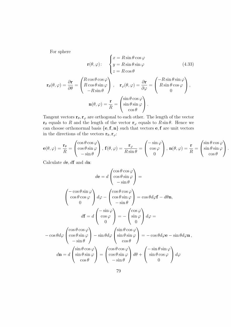
For sphere

r(θ, φ) :

x = R sin θ cosφ

y = R sin θ sinφ

z = R cos θ

(4.33)

rθ(θ, φ) =∂r

∂θ=


, rφ(θ, φ) =∂r

∂φ=


0

,

n(θ, φ) =r

R=


cos θ

.

Tangent vectors rθ, rφ are orthogonal to each other. The length of the vectorrθ equals to R and the length of the vector rφ equals to R sin θ. Hence wecan choose orthonormal basis {e, f ,n} such that vectors e, f are unit vectorsin the directions of the vectors rθ, rφ:

e(θ, φ) =rθR

=

cos θ cosφcos θ sinφ− sin θ

, f(θ, φ) =rφ

R sin θ=

− sinφcosφ0

, n(θ, φ) =r

R=


cos θ

.

Calculate de, df and dn:

de = d


=

− cos θ sinφcos θ cosφ

0

dφ−


= cos θdφf − dθn,

df = d

− sinφcosφ0

= −

cosφsinφ0

dφ =

− cos θdφ


− sin θdφ


cos θ

= − cos θdφe− sin θdφn ,

dn = d


cos θ

=


dθ +

− sin θ sinφsin θ cosφ

0

dφ

79

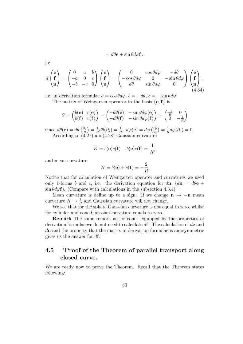
= dθe+ sin θdφf .

i.e.

d

efn

=

0 a b−a 0 c−b −c 0

efn

=

0 cos θdφ −dθ− cos θdφ 0 − sin θdφ

dθ sin θdφ 0

efn

,

(4.34)i.e. in derivation formulae a = cos θdφ, b = −dθ, c = − sin θdφ.

The matrix of Weingarten operator in the basis {e, f} is

S =

(b(e) c(e)b(f) c(f)

)=

(−dθ(e) − sin θdφ(e)−dθ(f) − sin θdφ(f)

)=

(−1R

00 − 1

R

)since dθ(e) = dθ

(∂θR

)= 1

Rdθ(∂θ) =

1R, dφ(e) = dφ

(∂θR

)= 1

Rdφ(∂θ) = 0.

According to (4.27) and(4.28) Gaussian curvature

K = b(e)c(f)− b(e)c(f) =1

R2

and mean curvature

H = b(e) + c(f) = − 2

R

Notice that for calculation of Weingarten operator and curvatures we usedonly 1-forms b and c, i.e. the derivation equation for dn, (dn = dθe +sin θdφf). (Compare with calculations in the subsection 4.3.4)

Mean curvature is define up to a sign. If we change n → −n meancurvature H → 1

Rand Gaussian curvature will not change.

We see that for the sphere Gaussian curvature is not equal to zero, whilstfor cylinder and cone Gaussian curvature equals to zero.

Remark The same remark as for cone: equipped by the properties ofderivation formulae we do not need to calculate df . The calculation of de anddn and the property that the matrix in derivation formulae is antisymmetricgives us the answer for df .

4.5 ∗Proof of the Theorem of parallel transport alongclosed curve.

We are ready now to prove the Theorem. Recall that the Theorem statesfollowing:

80

If C is a closed curve on a surface M such that C is a boundary of acompact oriented domain D ⊂ M , then during the parallel transport of anarbitrary tangent vector along the closed curve C the vector rotates throughthe angle

∆Φ = ∠ (X,RCX) =

∫D

Kdσ , (4.35)

where K is the Gaussian curvature and dσ =√det gdudv is the area element

induced by the Riemannian metric on the surface M , i.e. dσ =√det gdudv.

(see (4.6).Recall that for derivation formulae (5.13) we obtained structure equations

da+ b ∧ c = 0db+ c ∧ a = 0dc+ a ∧ a = 0

(4.36)

We need to use only one of these equations, the equation

da+ b ∧ c = 0 . (4.37)

This condition sometimes is called Gauß condition.Let as always {e, f ,n} be an orthonormal basis in TpE

3 at every pointof surface p ∈ M such that {e, f} is an orthonormal basis in TpM at everypoint of surface p ∈ M . Then the Gauß condition (4.37) and equation (4.27)mean that for Gaussian curvature on the surfaceM can be expressed throughthe 2-form da and base vectors {e, f}:

K = b ∧ c(e, f) = −da(e, f) (4.38)

We use this formula to prove the Theorem.Now calculate the parallel transport of an arbitrary tangent vector over

the closed curve C on the surface M .Let r = r(u, v) = r(uα) (α = 1, 2, (u, v) = (u1, v1)) be an equation of the

surface M .Let uα = uα(t) (α = 1, 2) be the equation of the curve C. Let X(t) be

the parallel transport of vector field along the closed curve C, i.e. X(t) istangent to the surface M at the point u(t) of the curve C and vector fieldX(t) is covariantly constant along the curve:

∇X(t)

dt= 0

81

To write this equation in components we usually expanded the vector fieldin the coordinate basis {ru = ∂u, rv = ∂v} and used Christoffel symbols ofthe connection Γα

βγ : ∇β∂γ = Γαβγ∂α.

Now we will do it in different way: instead coordinate basis {ru = ∂u, rv =∂v} we will use the basis {e, f}. In the subsection 3.4.4 we obtained that theconnection ∇ has the following appearance in this basis

∇ve = a(v)f , ,∇vf = −a(v)e (4.39)

(see the equations (4.20) and (4.21))Let

X = X(u(t)) = X1(t)e(u(t)) +X2(t)f(u(t))

Lbe an expansion of tangent vector field X(t) over basis {e, f}. Let v be ve-

locity vector of the curve C. Then the equation of parallel transport ∇X(t)dt

= 0will have the following appearance:

∇X(t)

dt= 0 = ∇v

(X1(t)e(u(t)) +X2(t)f(u(t))

)=

dX1(t)

dte(u(t)) +X1(t)∇ve(u(t)) +

dX2(t)

dtf(u(t)) +X2(t)∇vf(u(t)) =

dX1(t)

dte(u(t)) +X1(t)a(v)f(u(t)) +

dX2(t)

dtf(u(t))−X2(t)a(v)e(u(t)) =(

dX1(t)

dt−X2(t)a(v)

)e(u(t)) +

(dX2(t)

dt+X1(t)a(v)

)f(u(t)) = 0.

Thus we come to equation:{X1(t)− a(v(t))X2 = 0

X2(t) + a(v(t))X1 = 0

There are many ways to solve this equation. It is very convenient to considercomplex variable

Z(t) = X1(t) + iX2(t)

We see that

Z(t) = X1(t) + iX2(t) = a(v(t))X2 − ia(v(t)X1 = −ia(v)Z(t),

82

i.e.dZ(t)

dt= −ia(v(t))Z(t) (4.40)

The solution of this equation is:

Z(t) = Z(0)e−i∫ t0 a(v(τ))dτ (4.41)

Calculate∫ t10

a(v(τ))dτ for closed curve u(0) = u(t1). Due to Stokes Theo-rem: ∫ t1

0

a(v(t))dt =

∫C

a =

∫D

da

Hence using Gauss condition (4.37) we see that∫ t1

0

a(v(t))dt =

∫C

a =

∫D

da = −∫D

b ∧ c

Claim ∫D

b ∧ c = −∫D

da =

∫Kdσ . (4.42)

Theorem follows from this claim:

Z(t1) = Z(0)e−i∫C a = Z(0)ei

∫D b∧C (4.43)

Denote the integral i∫Db ∧ C by ∆Φ: ∆Φ = i

∫Db ∧ C. We have

Z(t1) = X1(t1) + iX2(t1) =(X1(0) + iX2(0)

)ei∆Φ = (4.44)

It remains to prove the claim. The induced volume form dσ is 2-form.Its value on two orthogonal unit vector e, f equals to 1:

dσ(e, f) = 1 (4.45)

(In coordinates u, v volume form dσ =√det gdu ∧ dv).

The value of the form b∧ c on vectors {e, f} equals to Gaussian curvatureaccording to (4.38). We see that

b ∧ c(e, f) = −da(e, f) = Kdσ(e, f)

Hence 2-forms b∧c, −da and volume form dσ coincide. Thus we prove (4.42).

83

5 Curvtature tensor

5.1 Definition

LetX,Y,Z be an arbitrary vector fields on the manifold equipped with affineconnection ∇.

Consider the following operation which assings to the vector fields X,Yand Z the new vector field.

R(X,Y)Z =(∇X∇Y −∇Y∇X −∇[X,Y]

)Z (5.1)

This operation is obviously linear over the scalar coefficients and it is C∞(M)with respect to vector fields X,YZ, i.e. for an arbitrary functions f, g, h

R(fX, gY)(hZ) = fghR(X,Y)Z, (5.2)

i.e. it defines the tensor field of the type

(13

): If X = X i∂i,X = X i∂i,X =

X i∂i then according to (5.2)

R(X,Y)Z = R(Xm∂m, Yn∂n)(Z

r∂r) = ZrRirmnX

mY n

where we denote by Rirmn the components of the tensor R in the coordinate

basis ∂iRi

rmn∂i = R(∂m, ∂n)∂r (5.3)

Express components of the curvature tensor in terms of Christoffel symbolsof the connection. If ∇m∂n = Γr

mn∂r then according to the (5.1) we have:

Rirmn∂i = R(∂m, ∂n)∂r = ∇∂m∇∂n∂r −∇∂n∇∂m∂r,

Rirmn = ∇∂m (Γp

nr∂p)−∇∂n (Γpmr∂p) =

∂mΓinr + Γi

mpΓpnr − (m ↔ n) (5.4)

The proof of the property (5.2) can be given just by straightforwardcalculations: Consider e.g. the case f = g = 1, then

R(X,Y)(hZ) = ∇X∇Y(hZ)−∇Y∇X(hZ)−∇[X,Y](hZ) =

∇X (∂YhZ+ h∇YZ)−∇Y (∂XhZ+ h∇XZ)− ∂[X,Y]hZ− h∇[X,Y]Z =

∂X∂YhZ+ ∂Yh∇XZ+ ∂Xh∇YZ+ h∇X∇YZ−

84

∂Y∂XhZ− ∂Xh∇YZ− ∂Yh∇XZ+ h∇Y∇XZ−

∂[X,Y]hZ− h∇[X,Y]Z =

h[∇X∇YZ−∇Y∇XZ)−∇[X,Y]Z

]+[∂X∂Yh− ∂Y∂Xh− ∂[X,Y]h

]Z =

h∇X∇YZ−∇Y∇XZ)−∇[X,Y]Z = hR(X,Y)Z ,

since ∂X∂Yh− ∂Y∂Xh− ∂[X,Y]h = 0.

5.1.1 Properties of curvature tensor

Tensor Rikmn is expressed trough derivatives of Christoffel symbols. In spite

this fact it is is much more ”pleasant” object than Christoffel symbols, sincethe latter is not the tensor.

It follows from the definition that the tensor Rikmn is antisymmetrical

with respect to indices m,n:

Rikmn = −Ri

knm . (5.5)

One can prove that for symmetric connection this tensor obeys the following identities:

Rikmn +Ri

mnk +Rinkm = 0 , (5.6)

The curvature tensor corresponding to Levi-Civita connection obeys alsoanother identities too (see the next subsection.)

We know well that If Christoffel symbols vanish in a vicinity of a givenpoint p in some chosen coordinate system then in general Christoffel symbolsdo not vanish in arbitrary coordinate systems. E.g. Christoffel symbols ofcanonical flat connection in E2 vanish in Cartesian coordinates but do notvanish in polar coordinates. This unpleasant property of Christoffel symbolsis due to the fact that Christoffel symbols do not form a tensor.

In particular if a tensor vanishes in some coordinate system, then it van-ishes in arbitrary coordinate system too. This implies very simple but im-portant

Proposition If curvature tensor Rikmn vanishes in some coordinate sys-

tem, then it vanishes in arbitrary coordinate systems.

We see that if Christoffel symbols vanish in a vicinity of a given pointp in some chosen coordinate system then it Riemannian curvature tensorvanishes at the point p (see the formula (5.4)) and hence it vanishes at thepoint p in arbitrary coordinate system.

85

5.2 Riemann curvature tensor of Riemannian mani-folds.

Let M be Riemannian manifold equipped with Riemannian metric GIn this section we will consider curvature tensor of Levi-Civita connection

∇ of Riemannian metric G.The curvature tensor for Levi-Civita connection will be called later Rie-

mann curvature tensor, or Riemann tensor.Using Riemannian metric one can consider Riemann tensor with all low

indicesRikmn = gijR

jkmn (5.7)

Due to identities (5.5) and (5.6) for curvature tensor Riemann tensorobeys the following identities:

Rikmn = −Riknm , Rikmn +Rimnk +Rinkm = 0 (5.8)

Riemann curvature tensor which is curvature tensor for Levi-Civita con-nection obeys also the following identities:

Rikmn = −Rkimn , Rikmn = Rmnki . (5.9)

These condition lead to the fact that for 2-dimensional Riemannian man-ifold the Riemann curvature tensor of Levi-Civita connection has essentiallyonly one non-vanishing component: all components vanish or equal to compo-nent R1212up to a sign. Indeed consider for 2-dimensional Riemannian man-ifold Riemann tensor Rikmn, where i, k,m, n = 1, 2. Since antisymmetricitywith respect to third and fourth indices (Rikmn = −Riknm), Rik11 = Rik22 = 0and Rik12 = −Rik21. The same for first and second indices: since antisym-metricity with respect to the the first and second indices (R12mn = −R21mn),R11mn = R22mn = 0 and R12mn = −Rik21. If we denote R1212 = a then

R1212 = R2121 = a,R1221 = R2112 = −a

and all other components vanish.For Riemann tensor one can consider Ricci tensor,

Rmn = Rimin (5.10)

which is symmetrical tensor: Rmn = Rnm.

86

One can consider scalar curvature:

R = Riking

kn = gknRkn (5.11)

where gkn is Riemannian metric with indices above (the matrix ||gik|| isinverse to the matrix ||gil||).

Ricci tensor and scalar curvature play essential role for formulation of Ein-stein gravity equations. In particular the space without matter the Einstenequations have the following form:

Rik −1

Rgik = 0 . (5.12)

5.3 †Curvature of surfaces in E3.. Theorema Egregiumagain

Express Riemannian curvature of surfaces in E3 in terms of derivation formulae (5.13).Consider derivation formulae for the orthonormal basis {e, f ,n, } adjusted to the sur-

face M :

d

efn

=

0 a b−a 0 c−b −c 0

efn

, (5.13)

where as usual e, f ,n vector fields of unit length which are orthogonal to each otherand n is orthogonal to the surface M . As we know the induced connection on the surfaceM is defined by the formulae (4.20) and (4.21):

∇Ye = (de(Y))tangent = a(X)f ,∇Yf = (df(Y))tangent = −a(X)e , (5.14)

According to the definition of curvature calculate

R(e, f)e = ∇e∇fe−∇f∇ee−∇[e,f ]e .

Note that since the induced connection is symmetrical connection then:

∇ef −∇fe− [e, f ] = 0 . (5.15)

hence due to (5.14)

[e, f ] = ∇ef −∇fe = a(e)e+ a(f)f (5.16)

Thus we see that R(e, f)e =

∇e∇fe−∇f∇ee−∇[e,f ]e = ∇e (a(f)f)−∇f (a(e)f)−∇a(e)e+a(f)fe =

∂ea(f)f + a(f)∇ef − ∂fa(e)f − a(e)∇f f − a(e)∇ee− a(f)∇fe =

87

∂ea(f)f − a(f)a(e)e− ∂fa(e)f + a(e)a(f)e− a(e)a(e)f − a(f)a(f)f =

[∂ea(f)f − ∂fa(e)f − a ((e)e− a(f)f)] f = da(e, f)f .

Recall that we established in 4.38 that for Gaussian curvature K

K = b ∧ c(e, f) = −da(e, f)

Hence we come to the relation:

R(e, f)e = da(e, f) = −Kf . (5.17)

This means thatR2

112 = −K

(in the basis e, f), i.e. the scalar curvature

R = 2R1212 = 2K

We come to fundamental relation which claims that the Gaussian curvature (the magni-tude defined in terms of External observer) equals to the scalar curvature, the magnitudedefined in terms of Internal observer. This gives us the straightforward proof of TheoremaEgregium.

Below we will give the proof of Theorema Egregium by straightforward calcultaions.

5.4 Relation between Gaussian curvature and Riemanncurvature tensor. Straightforward proof of Theo-rema Egregium

Let M be a surface in E3 and Rikmp be Riemann tensor, Riemann curva-

ture tensor of Levi-Civita connection. Recall that this means that Rikmp

is curvature tensor of the connection ∇, which is Levi-Civita connection ofthe Riemannian metric gαβ induced on the surface M by standard Euclideanmetric dx2 + dy2 + dz2. Recall that Riemann curvature tensor is expressedvia Christoffel symbols of connection by the formula

Rikmn = ∂mΓ

ink + Γi

mpΓpnk − ∂nΓ

imk − Γi

npΓpmk (5.18)

(see he formula (5.4)) where Christoffel symbols of Levi-Civita connectionare defined by the formula

Γimk =

1

2gij(∂gjm∂xk

+∂gjk∂xm

− ∂gmk

∂xj

)(5.19)

(see Levi-Civita Theorem)

88

Recall that scalar curvature R of Riemann tensor equals to R = Rikimg

km,where gkm is Riemannina metric tensor with upper indices (matrix ||gik|| isinverse to the matrix ||gik||). Note that as it was mentioned before theformula for scalar curvature becomes very simple in two-dimensional case (seeformulae (5.8) and (5.8) above). Using these formulae calculate Ricci tensorand scalar curvature R. Let R1212 = a. We know that all other componentsof Riemann tensor equal to zero or equal to ±a (see (5.8) and (5.8)). One canshow that scalar curvature R can be expressed via the component R1212 = aby the formula

R =2R1212

det g(5.20)

where det g = det gik = g11g22 = g212.Show it. Using identities (5.8) and (5.8) we see that

R11 = Ri1i1 = R2

121 = g22R2121 + g21R1121 = g22R1212 = g22a (5.21)

R22 = Ri2i2 = R1

212 = g11R1212 + g12R2221 = g11R1212 = g11a (5.22)

R12 = R21 = Ri1i2 = R1

112 = g12R2112 = −g12R1212 = −g12a (5.23)

Thus

Rik =

(g22a −g12a−g21a g11a

)Now for scalar curvature we have

R = Rikimgkm = Rkmgkm = g11R11 + g12R12 + g21R21 + g22R22 = (5.24)

2R1212(g11g22 − g12g12) = 2a det g−1 =

2a

det g

Now we formulate very importantProposition For an arbitrary point of the surface M

R = 2K (5.25)

where R = Rikimg

km is scalar curvature and K is Gaussian curvature.We know also that for surface M the scalar curvature R is expressed

via Riemann curvature tensor by the formula (5.20). Hence if we knowthe Gaussian curvature then we know all components of Riemann curvaturetensor (since all components vanish or equal to ±a.): using (5.20) one canrewrite the formula (5.25)

R1212

det g= K (5.26)

89

This is nothing but Theorema Egregium! Indeed Theorema Egregium(see beginning of the section 4) immediately follows from this Proposition.Indeed according to the formulae (5.18) and (5.19) the left hand side ofthe relation R = 2K depends only on induced Riemannian metric. HenceGaussian curvature K depends only on induced Riemannian metric.

It remains to prove the Proposition. We do it by direct calculations inthe next subsection.

Example LetM = S2 be sphere of radius R in E3. Show that one cannotfind local coordinates u, v on the sphere such that induced Riemannian metricequals to du2 + dv2 in these coordinates.

This immediately follows from the Proposition. Indeed suppose there ex-ist local coordinates u, v on the sphere such that induced Riemannian metricequals to du2 + dv2, i.e. Riemannian metric is given by unity matrix. Thenaccording to the formulae for Levi-Civita connection, the Christoffel symbolsequal to zero in these coordinates. Hence Riemann curvature tensor equalsto zero, and scalar curvature too. Due to Proposition this is in contradictionwith the fact that Gaussian curvature of the sphere equals to 1

R2 .

5.4.1 ∗Proof of the Proposition (5.25)

We prove this fact by direct calculations. The plan of calculations is following:Let M be a surface in E3 For an arbitrary point p of the surface M we

consider cartesian coordinates x, y, z such that orgin coincides with the pointp and coordinate plane OXY is the palne attached at the surface at thepoint p and the axis OZ is orthogonal to the surface. In these coordinatescalculations become easy. The surface M in these Cartesian coordinates canbe expressed by the equation

x = u

y = v

z = F (u, v)

(5.27)

where F (u, v) has local extremum at the point u = v = 014.

14more in detail this is stationary point. It is local extremum if quadratic form corre-sponding to second differential is positive or negative definite, i.e. FuuFvv −F 2

uv keeps thesign. This means that the Gaussian curvature is not negative

90

Calculate explicitly Gaussian curvature at the point p. In a vicinity of

the point p basis vector ru =

10Fu

, basis vector rv =

01Fv

. One can see

that

n(u, v) =1

1 + F 2u + F 2

v

−Fu

−Fv

1

(5.28)

is unit normal vector. In particular in the origin at the point p, we have

ru =

100

, rv =

010

, and n =

001

(5.29)

Now calculate shape operator. We need this operator only at the origin,hence during calculations of all derivatives we have to note that we needthe final result only at the point u = v = 0. This will essentially simplifycalculations since at the point p derivatives Fu, Fv equal to zero.

Sru = −∂un(u, v)|p = − ∂

∂u

1

1 + F 2u + F 2

v

−Fu

−Fv

1

|u=v=0 =

Fuu

−Fvu

1

|u=v=0 = Fuuru + Fuvrv

and

Srv = −∂vn(u, v)|p = − ∂

∂v

1

1 + F 2u + F 2

v

−Fu

−Fv

1

|u=v=0 =

Fuv

−Fvv

1

|u=v=0 = Fuvru + Fvvrv

since Fu = Fv = 0. We see that at the origin the Shape (Weingarten)operator equals to

S =

(Fuu Fuv

Fvu Fvv

)(5.30)

91

(all the derivatives at the origin).Gaussian curvature at the point p equals to

K = detS = FuuFvv − F 2uv . (5.31)

(all the derivatives at the origin).Now it is time to calculate the Riemann curvature tensor at the origin.First of all recall the expression for Riemannian metric for the surface M

in a vicinity of origin is

G =

(⟨ru, ru⟩ ⟨ru, rv⟩⟨rv, ru⟩ ⟨rv, rv⟩

)=

(1 + F 2

u FuFv

FvFu 1 + F 2v

). (5.32)

This immediately follows from the expression for basic vectors ru, rvNote that Riemannian metric gik at the point u = v = 0 is defined by

unity matrix guu = gvv = 1, guv = gvu = 0 since p is extremum point:

G =

(1 + F 2

u FuFv

FvFu 1 + F 2v

) ∣∣p=

(1 00 1

)since p is stationary point, extremum

(Fu = Fv = 0). Hence the components of the tensor Rikmn and Rikmn =

gijRjkmn at the point p are the same.

Recall that the components of Rikmn are defined by the formula

Rikmn = ∂mΓ

ink + Γi

mpΓpnk − ∂nΓ

imk − Γi

npΓpmk .

Notice that at the point p not only the matrix of the metric gik equals to unitymatrix, but more: Christoffel symbols vanish at this point in coordinates u, vsince the derivatives of metric at this point vanish. (Why they vanish: thisimmediately follows from Levi-Civita formula applied to the metric (5.32),see also in detail the file ”The solution of the problem 5 in the coursework,revisited”). Hence to calculate Ri

kmn at the point p one can consider moresimple formula:

Rikmn|p = ∂mΓ

ink|p − ∂nΓ

imk|p

Try to calculate in a more ”economical” way. Due to Levi-Civita formula

Γimk =

1

2gij(∂gjm∂xk

+∂gjk∂xm

− ∂gmk

∂xj

)Since metric gik equals to unity matrix g =

(1 00 1

)at the point p hence gij

is unity matrix also:

gik|p =

(1 00 1

)= δik .

92

(We denote δik the unity matrix: all diagonal components equal to 1, all othercomponents equal to zero. (It is so called Kronecker symbols)) Moreover weknow also that all the first derivatives of the metric vanish at the point p:

∂gik∂xm

|p = 0 .

Hence it follows from the formulae above that for an arbitrary indices i, j, k,m, n

∂

∂xi

(gkm

∂gpr∂xj

) ∣∣p=

∂gkm

∂xi

∣∣p

∂gpr∂xj

∣∣p+ gkm

∣∣p

∂2gpr∂xi∂xj

∣∣p= δkm

∂2gpr∂xi∂xj

∣∣p.

Now using the Levi-Civita formula for the Christoffel symbols of connection:

Γimk =

1

2gij(∂gjm∂xk

+∂gjk∂xm

− ∂gmk

∂xj

)we come to ∂nΓ

imk|p = ∂

∂xn

(12gij(

∂gjm∂xk +

∂gjk∂xm − ∂gmk

∂xj

)) ∣∣p=

1

2δij(

∂2gjm∂xn∂xk

+∂2gjk

∂xn∂xm− ∂2gmk

∂xn∂xj

) ∣∣p. (5.33)

Now using this formula we are ready to calculate Riemann curvature tensorRi

kmn. Remember that it is enough to calculate R1212 and R1

212 = R1212 atthe point p since gik = δik at the point p. We have that at p R1

212|p =∂1Γ

122|p − ∂2Γ

112|p and according to (5.33)

∂1Γ122 =

1

2δ1j(

∂2gj2∂x1∂x2

+∂2gj2∂x1∂x2

− ∂2g22∂x1∂xj

) ∣∣p=

1

2

(∂2g12∂x1∂x2

+∂2g12∂x1∂x2

− ∂2g22∂x1∂x1

) ∣∣p=

∂2g12∂x1∂x2

− 1

2

∂2g22∂x1∂x1

∣∣p,

∂2Γ112 =

1

2δ1j(

∂2gj1∂x2∂x2

+∂2gj2∂x2∂x1

− ∂2g12∂x2∂xj

) ∣∣p=

1

2

(∂2g11∂x2∂x2

+∂2g12∂x2∂x1

− ∂2g12∂x2∂x1

) ∣∣p=

1

2

∂2g11∂x2∂x2

∣∣p,

Hence

R1212|p = R1212|p = ∂1Γ

122|p−∂2Γ

112|p =

(∂2g12∂x1∂x2

− 1

2

∂2g22∂x1∂x1

− 1

2

∂2g11∂x2∂x2

) ∣∣p

93

Now using expression (5.32) for metric calculate second derivatives ∂2g12∂x1∂x2 ,

∂2g11∂x2∂x2

and ∂2g22∂x1∂x1 :

∂2g12∂x1∂x2

|p =∂2(FuFv)

∂u∂v

∣∣p=

∂

∂u(FuFvv + FuvFv) |p =

(FuuFvv + F 2

uv

)|p .

since Fu = Fv = 0 at the extremum point p (x1 = u, x2 = v). Analogoulsy

∂2g11∂x2∂x2

|p =∂2(1 + F 2

u )

∂v∂v

∣∣p=

∂

∂v(2FuFuv) |p = 2F 2

uv|p

and∂2g22∂x1∂x1

|p =∂2(1 + F 2

v )

∂u∂u

∣∣p=

∂

∂u(2FvFuv) |p = 2F 2

uv|p ,

We have finally that

R1212|p = R1212|p = ∂1Γ

122|p−∂2Γ

112|p =

(∂2g12∂x1∂x2

− 1

2

∂2g22∂x1∂x1

− 1

2

∂2g11∂x2∂x2

) ∣∣p= FuuFvv−F 2

uv .

The scalar curvature according to (5.20) equals to R = 2R1212 = 2(FuuFvv −F 2uv). Comparing with the expressionK = FuuFvv−F 2

uv in (5.31) for Gaussiancurvature we come to R = 2K .

5.5 Gauss Bonnet Theorem

Consider the integral of curvature over whole closed surface M . Accordingto the Theorem above the answer has to be equal to 0 (modulo 2π), i.e. 2πNwhere N is an integer, because this integral is a limit when we consider verysmall curve. We come to the formula:∫

D

Kdσ = 2πN

(Compare this formula with formula (4.6)).What is the value of integer N?We present now one remarkable Theorem which answers this question

and prove this Theorem using the formula (4.6).

94

Let M be a closed orientable surface.15 All these surfaces can be clas-sified up to a diffeomorphism. Namely arbitrary closed oriented surface Mis diffeomorphic either to sphere (zero holes), or torus (one hole), or pretzel(two holes),... ”Number k” of holes is intuitively evident characteristic of thesurface. It is related with very important characteristic—Euler characteristicχ(M) by the following formula:

χ(M) = 2(1− g(M)), where g is number of holes (5.34)

Remark What we have called here ”holes” in a surface is often referredto as ”handles” attached o the sphere, so that the sphere itself does not haveany handles, the torus has one handle, the pretzel has two handles and soon. The number of handles is also called genus.

Euler characteristic appears in many different way. The simplest appear-ance is the following:

Consider on the surface M an arbitrary set of points (vertices) connectedwith edges (graph on the surface) such that surface is divided on polygonswith (curvilinear sides)—plaquets. (”Map of world”)

Denote by P number of plaquets (countries of the map)Denote by E number of edges (boundaries between countries)Denote by V number of vertices.Then it turns out that

P − E + V = χ(M) (5.35)

It does not depend on the graph, it depends only on how much holes hassurface.

E.g. for every graph on M , P − E + V = 2 if M is diffeomorphic tosphere. For every graph on M P −E+V = 0 if M is diffeomorphic to torus.

Now we formulate Gauß -Bonnet Theorem.Let M be closed oriented surface in E3.Let K(p) be Gaussian curvature at any point p of this surface.

15Closed means compact surface without boundaries. Intuitively orientability meansthat one can define out and inner side of the surface. In terms of normal vectors ori-entability means that one can define the continuous field of normal vectors at all thepoints of M . The direction of normal vectors at any point defines outward direction.Orientable surface is called oriented if the direction of normal vector is chosen.

95

Theorem (Gauß -Bonnet) The integral of Gaussian curvature over theclosed compact oriented surface M is equal to 2π multiplied by the Eulercharacteristic of the surface M

1

2π

∫M

Kdσ = χ(M) = 2(1− number of holes) (5.36)

In particular for the surface M diffeomorphic to the sphere κ(M) = 2,for the surface diffeomorphic to the torus it is equal to 0.

The value of the integral does not change under continuous deformationsof surface! It is integer number (up to the factor π) which characterisestopology of the surface.

E.g. consider surface M which is diffeomorphic to the sphere. If it issphere of the radius R then curvature is equal to 1

R2 , area of the sphere isequal to 4πR2 and left hand side is equal to 4π

2π= 2.

If surface M is an arbitrary surface diffeomorphic to M then metrics andcurvature depend from point to the point, Gauß -Bonnet states that integralnevertheless remains unchanged.

Very simple but impressive corollary:Let M be surface diffeomorphic to sphere in E3. Then there exists at least

one point where Gaussian curvature is positive.Proof: Suppose it is not right. Then

∫MK√det gdudv ≤ 0. On the other

hand according to the Theorem it is equal to 4π. Contradiction.

Proof of Gauß-Bonet TheoremConsider triangulation of the surface M . Suppose M is covered by N triangles. Then

number of edges will be 3N/over2. If V number of vertices then according to EulerTheorem

N − 3N

2+ V = V − N

2= χ(M).

Calculate the sum of the angles of all triangles. On the one hand it is equal to 2πV . Onthe other hand according the formula (4.6) it is equal to

N∑i=1

(π +

∫△i

Kdσ

)= πN +

N∑i=1

(∫△i

Kdσ

)= Nπ +

∫M

Kdσ

We see that 2πV = Nπ +∫M

Kdσ, i.e.∫M

Kdσ = π

(2V − N

2

)= 2πχ(M)

96

6 Appendices

6.1 ∗Integrals of motions and geodesics.

We see how useful in Riemannian geometry to use the Lagrangian approach.To solve and study solutions of Lagrangian equations (in particular geodesics which

are solutions of Euler-Lagrange equations for Lagrangian of free particle) it is very usefulto use integrals of motion

6.1.1 ∗Integral of motion for arbitrary Lagrangian L(x, x)

Let L = L(x, x) be a Lagrangian, the function of point and velocity vectors on manifoldM (the function on tangent bundle TM).

Definition We say that the function F = F (q, q) on TM is integral of motion forLagrangian L = L(x, x) if for any curve q = q(t) which is the solution of Euler-Lagrangeequations of motions the magnitude I(t) = F (x(t), x(t)) is preserved along this curve:

F (x(t), x(t)) = const if x(t) is a solution of Euler-Lagrange equations(3.9). (6.1)

In other words

d

dt(F (x(t), x(t))) = 0 if xi(t) :

d

dt

(∂L

∂xi

)− ∂L

∂xi= 0 . (6.2)

6.1.2 ∗Basic examples of Integrals of motion: Generalised momen-tum and Energy

Let L(xi, xi) does not depend on the coordinate x1. L = L(x2, . . . , xn, x1, x2, . . . , xn).Then the function

F1(x, x) =∂L

∂x1

is integral of motion. (In the case if L(xi, xi) does not depend on the coordinate xi. thefunction Fi(x, x) =

∂L∂xi

will be integral of motion.)

Proof is simple. Check the condition (6.2): Euler-Lagrange equations of motion are:

d

dt

(∂L

∂xi

)− ∂L

∂xi= 0 (i = 1, 2, . . . , n)

We see that exactly first equation of motion is

d

dt

(∂L

∂x1

)=

d

dtF1(q, q) = 0 since ∂L

∂x1 = 0, .

(if L(xi, xi) does not depend on the coordinate xi then the function Fi(x, x) =∂Lx1 is

integral of motion since i− th equation is exactly the condition Fi = 0.)The integral of motion Fi =

∂L∂xi

is called sometimes generalised momentum.

97

Another very important example of integral of motion is: energy.

E(x, x) = xi ∂L

∂xi− L . (6.3)

One can check by direct calculation that it is indeed integral of motion. Using Euler

Lagrange equations ddt

(∂L∂xi

)− ∂L

∂xi we have:

d

dtE(x(t), x(t)) =

d

dt

(xi ∂L

∂xi− L

)=

∂L

∂xi

dxi

dt+

d

dt

(∂L

∂xi

)xi − dL

dt=

∂L

∂xi

dxi

dt+

∂L

∂xi

dxi

dt− dL(x, x)

dt=

dL(x, x)

dt− dL(x, x)

dt= 0 .

6.1.3 ∗Integrals of motion for geodesics

Apply the integral of motions for studying geodesics.

The Lagrangian of ”free” particle Lfree = gik(x)xixk

2 . For Lagrangian of free particlesolution of Euler-Lagrange equations of motions are geodesics.

If F = F (x, x) is the integral of motion of the free Lagrangian Lfree =gik(x)x

ixk

2 thenthe condition (6.1) means that the magnitude I(t) = F (xi(t), xi(t)) is preserved along thegeodesics:

I(t) = F (xi(t), xi(t)) = const, i.e.d

dtI(t) = 0 if xi(t) is geodesic. (6.4)

Consider examples of integrals of motion for free Lagrangian, i.e. magnitudes whichpreserve along the geodesics:

Example 1 Note that for an arbitrary ”free” Lagrangian Energy integral (6.3) is anintegral of motion:

E = xi ∂L

∂xi− L = xi

∂(

gpq(x)xpxq

2

)∂xi

− gik(x)xixk

2=

xigiq(x)xq − gik(x)x

ixk

2=

gik(x)xixk

2. (6.5)

This is an integral of motion for an arbitrary Riemannian metric. It is preserved on anarbitrary geodesic

dE(t)

dt=

d

dt

(1

2gik(x(t))x

i(t)xk(t)

)= 0 .

In fact we already know this integral of motion: Energy (6.5) is proportional to the squareof the length of velocity vector:

|v| =√

gik(x)xixk =√2E . (6.6)

We already proved that velocity vector is preserved along the geodesic (see the Propositionin the subsection 3.2.1 and its proof (??).)

98

Example 2 Consider Riemannian metric G = adu2 + bdv2 (see also calculations insubsection 2.3.3) in the case if a = a(u), b = b(u), i.e. coefficients do not depend on thesecond coordinate v:

G = a(u)du2 + b(u)dv2, Lfree =1

2

(a(u)u2 + b(u)v2

)(6.7)

We see that Lagrangian does not depend on the second coordinate v hence the magnitude

F =∂Lfree

∂v= b(u)v (6.8)

is preserved along geodesic. It is integral of motion because Euler-Lagrange equation forcoordinate v is

d

dt

∂Lfree

∂v− ∂Lfree

∂v=

d

dt

∂Lfree

∂v=

d

dtF = 0 since ∂Lfree

∂v = 0. .

In fact all revolution surfaces which we consider here (cylinder, cone, sphere,...) haveRiemannian metric of this type. Indeed consider further examples.

Example (sphere)Sphere of the radius R in E3. Riemannian metric: G = Rdθ2 + R2 sin2 θdφ2 and

Lfree = 12

(R2θ2 +R2 sin2 θφ2

)It is the case (6.7) for u = θ, v = φ, b(u) = R2 sin2 θ The

integral of motion is

F =∂Lfree

∂φ= R2 sin2 θφ

Example (cone)

Consider cone

x = ah cosφ

y = ah sinφ

z = bh

. Riemannian metric:

G = d(ah cosφ)2 + d(ah sinφ)2 + (dbh)2 = (a2 + b2)dh2 + a2h2dφ2 .

and free Lagrangian

Lfree =(a2 + b2)h2 + a2h2φ2

2.

The integral of motion is

F =∂Lfree

∂φ= a2h2φ.

Example (general surface of revolution)Consider a surface of revolution in E3:

r(h, φ) :

x = f(h) cosφ

y = f(h) sinφ

z = h

(f(h) > 0) (6.9)

99

(In the case f(h) = R it is cylinder, in the case f(h) = kh it is a cone, in the casef(h) =

√R2 − h2 it is a sphere, in the case f(h) =

√R2 + h2 it is one-sheeted hyperboloid,

in the case z = cosh it is catenoid,...)For the surface of revolution (6.9)

G = d(f(h) cosφ)2 + d(f(h) sinφ)2 + (dh)2 = (f ′(h) cosφdh− f(h) sinφdφ)2+

(f ′(h) sinφdh+ f(h) cosφdφ)2 + dh2 = (1 + f ′2(h))dh2 + f2(h)dφ2 .

The ”free” Lagrangian of the surface of revolution is

Lfree =

(1 + f ′2(h)

)h2 + f2(h)φ2

2.

and the integral of motion is

F =∂Lfree

∂φ= f2(h)φ.

6.1.4 ∗Using integral of motions to calculate geodesics

Integrals of motions may be very useful to calculate geodesics. The equations for geodesicsare second order differential equations. If we know integrals of motions they help us tosolve these equations. Consider just an example.

For Lobachevsky plane the free Lagrangian L = x2+y2

2y2 . We already calculated geodesicsin the subsection 3.3.4. Geodesics are solutions of second order Euler-Lagrange equations

for the Lagrangian L = x2+y2

2y2 (see the subsection 3.3.4){··x− 2xy

y = 0··y + x2

y − y2

y = 0

It is not so easy to solve these differential equations.For Lobachevsky plane we know two integrals of motions:

E = L =x2 + y2

2y2, and F =

∂L

∂x=

x

y2. (6.10)

These both integrals preserve in time: if x(t), y(t) is geodesics then{F = x(t)

y(t)2

E = x(t)2+y(t)2

2y(t)2 = C2

⇒

{x = C1y

2

y = ±√

2C2y2 − C21y

4

These are first order differential equations. It is much easier to solve these equations ingeneral case than initial second order differential equations.

100

6.2 Induced metric on surfaces.

Recall here again induced metric (see for detail subsection 1.4)If surface M : r = r(u, v)is embedded in E3 then induced Riemannian metric GM is

defined by the formulae

⟨X,Y⟩ = GM (X,Y) = G(X,Y) , (6.11)

where G is Euclidean metric in E3:

GM = dx2 + dy2 + dz2∣∣r=r(u,v)

=3∑

i=1

(dxi)2∣∣r=r(u,v)

=3∑

i=1

(∂xi

∂uαduα

)2

=∂xi

∂uα

∂xi

∂uβduαduβ ,

i.e.

GM = gαβduα, where gαβ =

∂xi

∂uα

∂xi

∂uβduαduβ .

We use notations x, y, z or xi (i = 1, 2, 3) for Cartesian coordinates in E3, u, v or uα

(α = 1, 2) for coordinates on the surface. We usually omit summation symbol over dummyindices. For coordinate tangent vectors

∂

∂uα︸︷︷︸Internal observer

= rα =∂xi

∂uα

∂

∂xi︸︷︷︸External observer

We have already plenty examples in the subsection 1.4. In particular for scalar product

gαβ =

⟨∂

uα,∂

uβ

⟩= xiαxiβ .⟨rα, rβ⟩ . (6.12)

6.2.1 Recalling Weingarten operator

Continue to play with formulae 16.Recall the Weingarten (shape) operator which acts on tangent vectors:

SX = −∂Xn , (6.13)

where we denote by n-unit normal vector field at the points of the surface M : ⟨n, rα⟩ = 0,⟨n, rα⟩ = 1.

Now we realise that the derivative ∂XR of vector field with respect to another vectorfield is not a well-defined object: we need a connection. The formula ∂XR in Cartesiancoordinates, is nothing but the derivative with respect to flat canonical connection: If

16In some sense differential geometry it is when we write down the formulae expressingthe geometrical facts, differentiate these formulae then reveal the geometrical meaning ofthe new obtained formulae e.t.c.

101

we work only in Cartesian coordinates we do not need to distinguish between ∂XR and∇can.flat

X R. Sometimes with some abuse of notations we will use ∂XR instead ∇can.flatX R,

but never forget: this can be done only in Cartesian coordinates where Christoffel symbolsof flat canonical connection vanish:

∂XR = ∇can.flatX R in Cartesian coordinates .

So the rigorous definition of Weingarten operator is

SX = −∇can.flatX n , (6.14)

but we often use the former one (equation (6.13)) just remembering that this can be doneonly in Cartesian coordinates.

Recall that the fact that Weingarten operator S maps tangent vectors to tangentvectors follows from the property: ⟨n,X⟩ = 0 ⇒ X is tangent to the surface.

Indeed:

0 = ∂X⟨n,n⟩ = 2⟨∂Xn,n⟩ = −2⟨SX,n⟩ = 0 ⇒ SX is tangent to the surface

Recall also that normal unit vector is defined up to a sign, n → −n. On the other hand

if n is chosen then S is defined uniquely.

6.2.2 Second quadratic form

We define now the new object: second quadratic formDefinition. For two tangent vectors X,Y A(X,Y) is defined such that(

∇can.flatX Y

)⊥ = A(X,Y)n (6.15)

i.e. we take orthogonal component of the derivative of Y with respect to X.This definition seems to be very vague: to evaluate covariant derivative we have to

consider not a vector Y at a given point but the vector field. In fact one can see thatA(X,Y) does depend only on the value of Y at the given point.

Indeed it follows from the definition of second quadratic form and from the propertiesof Weingarten operator that

A(X,Y) =⟨(∇can.flat

X Y)⊥ ,n

⟩=⟨∇can.flat

X Y,n⟩=

∂X⟨Y,n⟩ −⟨Y,∇can.flat

X n⟩= ⟨S(X),Y⟩ (6.16)

We proved that second quadratic form depends only on value of vector field Y at thegiven poit and we established the relation between second quadratic form and Weingartenoperator.

Proposition The second quadratic form A(X,Y) is symmetric bilinear form on tan-gent vectors X,Y in a given point.

A : TpM ⊗ TpM → R, A(X,Y) = A(Y,X) = ⟨SX,Y⟩ . (6.17)

102

In components

A = Aαβduαduβ = ⟨rαβ ,n⟩ =

∂2xi

∂uα∂uβni . (6.18)

andSαβ = gαπAπβ = gαπxi

πβni , (6.19)

i.e.A = GS, S = G−1A .

Remark The normal unit vector field is defined up to a sign.

6.2.3 Gaussian and mean curvatures

Recall that Gaussian curvatureK = detS

and mean curvatureH = TrS

It is easy to see that for Gaussian curvature

K = detS = det(G−1A) =detA

detG.

We know already the geometrical meaning of Gaussian and mean curvatures from thepoint of view of the External Observer:

Gaussian curvature K equals to the product of principal curvatures, and mean cur-vartures equals to the sum of principal curvatures.

Now we ask a principal question: what bout internal observer, ”aunt” living on thesurface?

We will show that Gaussian curvature can be expressed in terms of induced Rieman-nian metric, i.e. it is an internal characteristic of the surface, invariant of isometries.

It is not the case with mean curvature: cylinder is isometric to the plane but it havenon-zero mean curvature.

6.2.4 Examples of calculation of Weingarten operator, Secondquadratic forms, curvatures for cylinder, cone and sphere.

Cylinder

We already calculated induced Riemannian metric on the cylinder (see (1.56)).Cylinder is given by the equation x2 + y2 = R2. One can consider the following

parameterisation of this surface:

r(h, φ) :

x = R cosφ

y = R sinφ

z = h

, rh =

001

, rφ =

−R sinφR cosφ

0

, (6.20)

103

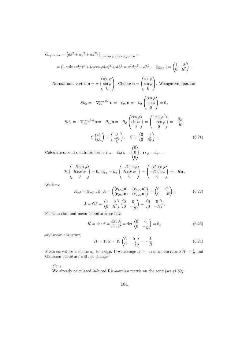
Gcylinder =(dx2 + dy2 + dz2

) ∣∣x=a cosφ,y=a sinφ,z=h

=

= (−a sinφdφ)2 + (a cosφdφ)2 + dh2 = a2dφ2 + dh2 , ||gαβ || =(1 00 R2

).

Normal unit vector n = ±

cosφsinφ0

. Choose n =

cosφsinφ0

. Weingarten operator

S∂h = −∇can.flatrh

n = −∂rhn = −∂h

cosφsinφ0

= 0 ,

S∂φ = −∇can.flatrφ n = −∂rφn = −∂φ

cosφsinφ0

=

sinφ− cosφ

0

= −∂φR

.

S

(∂h∂φ

)=

(0

−∂φ

R

), S =

(0 00 −1

R

). (6.21)

Calculate second quadratic form: rhh = ∂hrh =

000

, rhφ = rφh =

∂h

−R sinφR cosφ

0

= 0, rφφ = ∂φ

−R sinφR cosφ

0

=

−R cosφ−R sinφ

0

= −Rn .

We have

Aαβ = ⟨rαβ ,n⟩, A =

(⟨rhh,n⟩ ⟨rhφ,n⟩⟨rφh,n⟩ ⟨rφφ,n⟩

)=

(0 00 −R

), (6.22)

A = GS =

(1 00 R2

)(0 00 − 1

R

)=

(0 00 −R

),

For Gaussian and mean curvatures we have

K = detS =detA

detG= det

(0 00 − 1

R

)= 0 , (6.23)

and mean curvature

H = TrS = Tr

(0 00 − 1

R

)= − 1

R. (6.24)

Mean curvature is define up to a sign. If we change n → −n mean curvature H → 1R and

Gaussian curvature will not change.

ConeWe already calculated induced Riemannian metric on the cone (see (1.59).

104

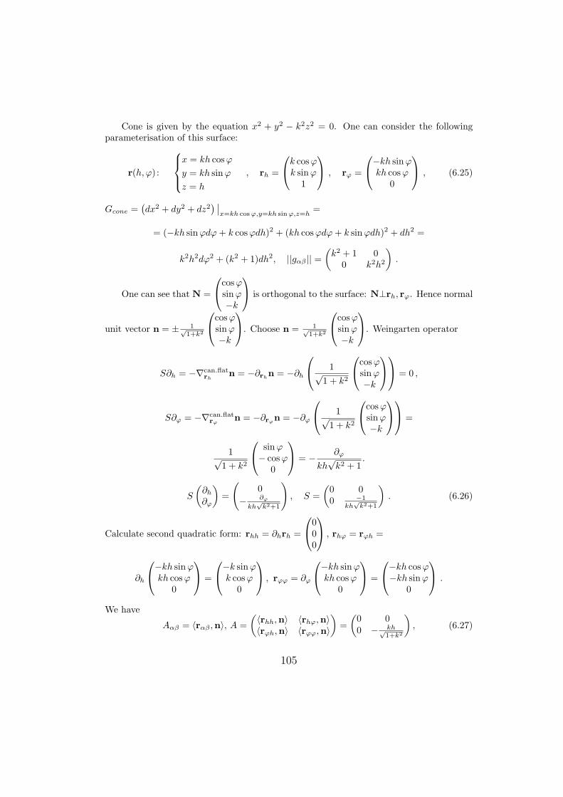
Cone is given by the equation x2 + y2 − k2z2 = 0. One can consider the followingparameterisation of this surface:

r(h, φ) :

x = kh cosφ

y = kh sinφ

z = h

, rh =

k cosφk sinφ

1

, rφ =

−kh sinφkh cosφ

0

, (6.25)

Gcone =(dx2 + dy2 + dz2


=

= (−kh sinφdφ+ k cosφdh)2 + (kh cosφdφ+ k sinφdh)2 + dh2 =

k2h2dφ2 + (k2 + 1)dh2, ||gαβ || =(k2 + 1 0

0 k2h2

).

One can see that N =

cosφsinφ−k

is orthogonal to the surface: N⊥rh, rφ. Hence normal

unit vector n = ± 1√1+k2

cosφsinφ−k

. Choose n = 1√1+k2

cosφsinφ−k


S∂h = −∇can.flatrh

n = −∂rhn = −∂h

1√1 + k2

cosφsinφ−k

= 0 ,

S∂φ = −∇can.flatrφ n = −∂rφn = −∂φ

1√1 + k2

cosφsinφ−k

=

1√1 + k2

sinφ− cosφ

0

= − ∂φ

kh√k2 + 1

.

S

(∂h∂φ

)=

(0

− ∂φ

kh√k2+1

), S =

(0 00 −1

kh√k2+1

). (6.26)

Calculate second quadratic form: rhh = ∂hrh =

000

, rhφ = rφh =

∂h

−kh sinφkh cosφ

0

=

−k sinφk cosφ

0

, rφφ = ∂φ

−kh sinφkh cosφ

0

=

−kh cosφ−kh sinφ

0

.

We have


(⟨rhh,n⟩ ⟨rhφ,n⟩⟨rφh,n⟩ ⟨rφφ,n⟩

)=

(0 00 − kh√

1+k2

), (6.27)

105

A = GS =

(k2 + 1 0

0 k2h2

)(0 00 −1

kh√k2+1

)=

(0 00 −kh√

k2+1

),


K = detS =detA

detG= det

(0 00 −1

kh√k2+1

)= 0 , (6.28)

and mean curvature

H = TrS = Tr

(0 00 −1

kh√k2+1

)=

−1

kh√k2 + 1

. (6.29)


Gaussian curvature will not change.

Sphere

Sphere is given by the equation x2 + y2 + z2 = a2. Consider the parameterisation ofsphere in spherical coordinates

r(θ, φ) :

x = R sin θ cosφ

y = R sin θ sinφ

z = R cos θ

(6.30)

We already calculated induced Riemannian metric on the sphere (see (6.2.4)). Recallthat

rθ =


, rφ =


0

and

GS2 =(dx2 + dy2 + dz2

) ∣∣x=R sin θ cosφ,y=R sin θ sinφ,z=R cos θ

=

(R cos θ cosφdθ −R sin θ sinφdφ)2 + (R cos θ sinφdθ +R sin θ cosφdφ)2+

(−R sin θdθ)2 = R2 cos2 θdθ2 +R2 sin2 θdφ2 +R2 sin2 θdθ2 =

= R2dθ2 +R2 sin2 θdφ2 , ||gαβ || =(R2 00 R2 sin2 θ

).

For the sphere r(θ, φ) is orthogonal to the surface. Hence normal unit vector n(θ, φ) =

± r(θ,φ)R = ±


cos θ

. Choose n = rR =


cos θ


S∂θ = −∇can.flatrθ

n = −∂θn = −∂θ

( r

R

)= −rθ

R,

S∂φ = −∇can.flatrφ n = −∂φn = −∂φ

( r

R

)= −rφ

R.

106

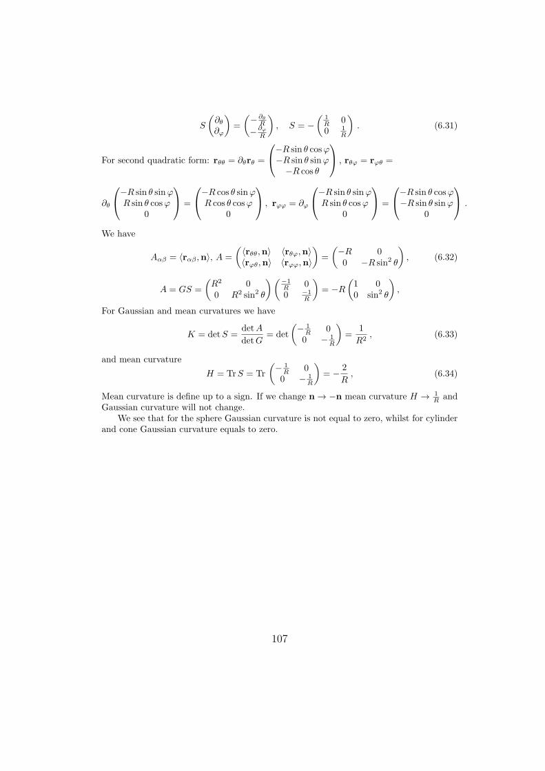
S

(∂θ∂φ

)=

(−∂θ

R

−∂φ

R

), S = −

(1R 00 1

R

). (6.31)

For second quadratic form: rθθ = ∂θrθ =


−R cos θ

, rθφ = rφθ =

∂θ


0

=


0

, rφφ = ∂φ


0

=


0

.

We have


(⟨rθθ,n⟩ ⟨rθφ,n⟩⟨rφθ,n⟩ ⟨rφφ,n⟩

)=

(−R 00 −R sin2 θ

), (6.32)

A = GS =

(R2 00 R2 sin2 θ

)(−1R 00 −1

R

)= −R

(1 00 sin2 θ

),


K = detS =detA

detG= det

(− 1

R 00 − 1

R

)=

1

R2, (6.33)

and mean curvature

H = TrS = Tr

(− 1

R 00 − 1

R

)= − 2

R, (6.34)


Gaussian curvature will not change.We see that for the sphere Gaussian curvature is not equal to zero, whilst for cylinder

and cone Gaussian curvature equals to zero.

107

Riemannian Geometry - University of Manchester

Documents

Transcript of Riemannian Geometry - University of Manchester