REVISTA 27 ENEROETICA - Centro de …biblioteca.olade.org/opac-tmpl/Documentos/hm000245.pdf · Si...

EL DESARROLLO DEL POTENCIAL HIDROELECTRICO DEL RIO CARONI ~ D[V[LOPING TH[: HYOROELfC l RlC POTE:NTIAL or THt Gt\RON 1 HIVH\ .. CARBON, LIGNITO Y TURBA EN BRASIL otcMM C01\l. 1 iUNllf: ANll Pi:AT IN fJRAZIL «** CUENCAS SEDIMENTARIAS Y POTENCIAL PETROLERO EN GUATEMALA .. SFOIME:NTARY BAS!NS 1\ND -HE O•L PO 1EN1 IAL O~ GUATEMALA --- MOLINOS DE VIENTO PARA BOMBEO DE ilGUA ~ WINUt/.lLLS FOR PUMPINS Wi\TER

Organización Latinoamericana de Energía Latin American Er 1ergy Org8.nization

Septiembre· Octubre/82 S~pter1..>~1 r..;t·ibe 182

REVISTA 27 ENEROETICA

Organización Latinoamericana de Energía

39

la densidad del aire a nivel del mar es más o menos 1,23 Kg./m3• Cada mil metros de altura se reduce un 10 o/o. A 4000 metros de altura p f::: 0,8 Kg./m3•

(*)

fuerza de sustentación, N fuerza de arrastre, N densidad del aire, (1,23 kg/m3 (*)) coeficiente de sustentación, adim. coeficiente de arrastre, adim. área elemental (cuerda x longitud diferencial de pala) velocidad del viento, m/seg

Donde:

dl = dD = p CL Co dA = voo

(2 2) dA

(2 - 1) dA do 1 Y2oo = Co.-p 2

DL 1 V200 = CL.-P 2

Cuando la pala de una aerobomba está bajo el efecto de una corriente de aire experimenta una fuerza. Si tomamos un elemento de pala esta fuerza se puede descom poner en la dirección del viento relativa y perpendicular a este, según se muestra en la Figura 38.

Los componentes en las direcciones relativa (do) y perpendicular (dL) a la direc .ión del viento pueden ser expresados por las siguientes relaciones matemáticas:

2.1.1 Geometría del Rotor

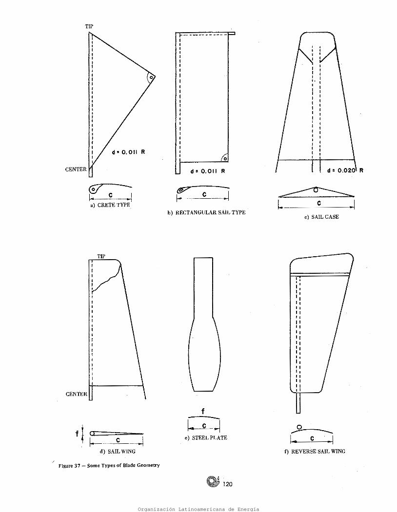
Existen diversas configuraciones de palas, como se puede observar en la Figura 37. En este documento sólo nos referimos al tipo plancha de acero (letra e de la figura); sin embargo en las referencias bibliográficas 2.5, 2.6 y 2.7 se podrá encontrar informa ción sobre molinos de viento construidos con rotores tipo CRETA (letra a de la figura), el que presenta una geometr(a sencilla y tiene interesantes caracterrsticas técnicas que Jo hacen especialmente atractivo en aplicaciones de riego.

2.1 CALCULO DEL ROTOR

CAPITULO 2 - DISEÑO DE UN SISTEMA DE BOMBEO DE EJE HORIZONTAL

2ª entrega

MOLINOS DE VIENTO PARA BOMBEO DE AGUA

'El presente documento forma parte de 4 entregas Sucesivas.


f) TIPO ALA DE VELA INVERSA

_..9_ ~e .. ¡

1 l 1 11 l 1 11 11 11 , ,

~

l.. e -1 e) FUNDA DE VELA

0)40 figura 37 Algunos Tipos de Geometría de Palas Utilizados

e) PLANCHA DE ACERO

f l .. e .. j

h) TIPO VELA RECTANGULAR

.1 - e-

d = 0.011 R

(P' ¡ ..

o

tl . ¡.. e .. ! d) ALA DE VELA

EXTREMO

er>: 1... e .. ¡ a) TIPO CRETA

d: 0.011 R

CENTRO

EXTREMO


41

Figura 39 Variación del Angulo Optimo de la Velocidad Relativa (</J} con la Relación de Velocidades en el Extremo de la Pala (Ao)

8 7 6 5 4 3 2 o >.o o -t-~---.-~~..-~-.--~--,,--~--.-~--.-~~.-~-.--~--é~

10

20

30

40

número de palas longitud de la cuerda (ver Fig. 37), m coeficiente de arrastre, adim. velocidad angular del rotor, rpm velocidad de diseño, m/seg.

60 Donde:

50

(2 - 3)

Aplicando la teoría del momentum y la ecuación de la energía a un elemento de pata e integrando a lo largo de la longitud de esta, se puede demostrar que para lograr la máxima transformación de la energía cinética del aire en mecánica de la pala, ésta debe tener una torsión tal que permita la presentación de un ángulo </) del viento relativo dada en la Fig. 39 y una longitud de cuerda que se ajuste a la función ¡/¡ , ver Fig. 40, dada por:

Figura 38 Efecto del Viento sobre un Elemento de Pala Woo


é 42

Para el rotor que nos interesa, consideramos por razones de construcción y costo, que vamos a usar planchas metálicas curvadas, con una sección como la que aparece en la Figura 41.

De la Figura 40 se deduce que la longitud de la cuerda aumenta hasta un máximo, cerca de A.0 = 1, y luego disminuye hacia el extremo de la misma.

cte pues se toma aquel para el cual la relación En la ecuación (2 4), ce (Co/CL) es mínima.;

[3 ángulo de la pala <P ángulo de la velocidad relativa a: ángulo de ataque del perfil

Donde:

(2 - 4) {J'=</J-0::

De la Figura 39 se deduce que la pala es muy abierta en la raíz y que este ángulo disminuye conforme nos acercamos a la punta, ya que según la Figura 38:

8 7 6 5 4 3 2 o

Figura 40 Variación de la Función iJ¡ con la Relación de Velocidades en el Extremo de la Pala (Ao) 5

3

4

6


43

Ao r (m) <P (o) ¡3 (o) 1./J e (m)

o. 1 . 125 56.2 52.2 . 17715 . 1035 0.2 .250 52.4 48.4 .31128 . 1819 0.4 .500 45.5 41.5 .47730 .2789 0.6 .750 39 .4 35.4 .54406 . 3179

0.8 1.000 34.5 30.5 .55430 . 3239 1.0 1.250 30.5 26.5 .53657 . 3135 1.2 1. 500 28.0 24.0 .5000 .. 2922 1. 4 1. 750 23.5 19.5 .4600 .2G88 1. 5 1.875 22.5 18.5 .45568 .2663 1.8 2.250 19.0 15.0 .4000 .2337 2.0 2.500 17. 8 13.8 . 38072 .2224

GEOMETRIA OPTIMA DE LA PALA

TABLA 13

Teniendo en cuenta estas consideraciones y realizando los cálculos indicados en la Tabla 13, podemos llegar a establecer la geometría óptima de la pala.

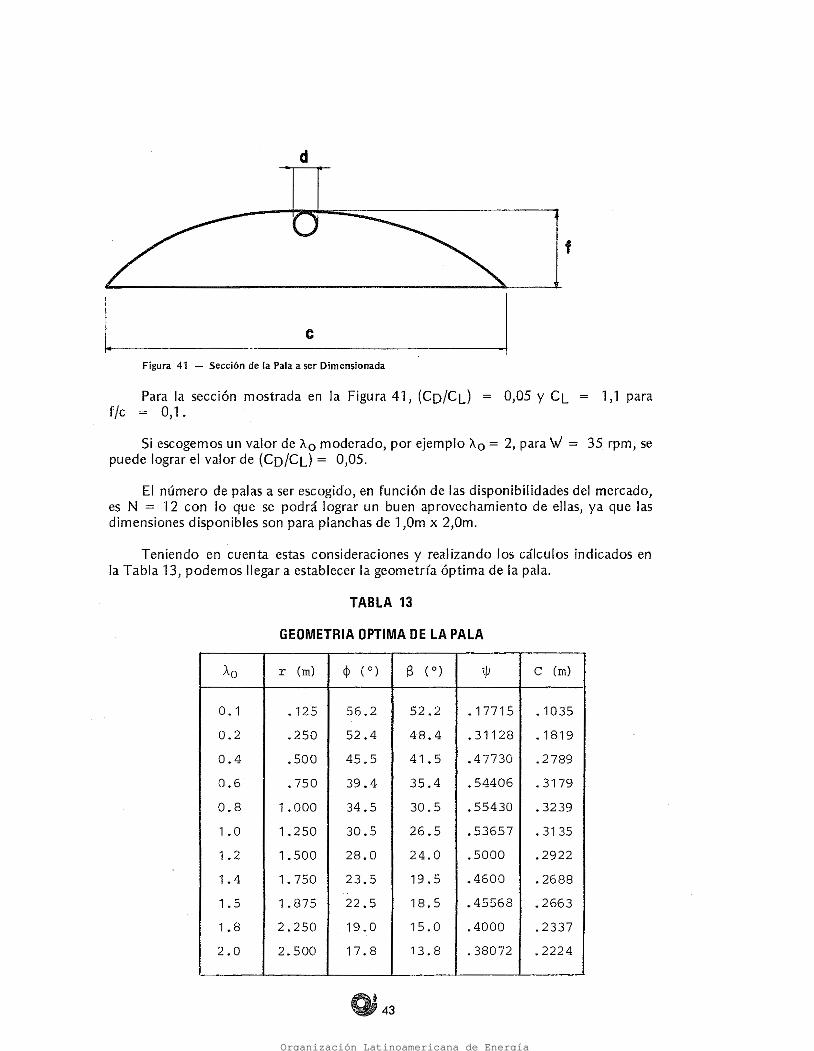
El número de palas a ser escogido, en función de las disponibilidades del mercado, es N = 12 con lo que se podrá lograr un buen aprovechamiento de ellas, ya que las dimensiones disponibles son para planchas de 1,0m x 2,0m.

Si escogemos un valor de ft.0 moderado, por ejemplo ft.0 = 2, para VI = 35 rprn, se puede lograr el valor de (Co/CL) = 0,05.

Para la sección mostrada en la Figura 41, (Co/CL) = 0,05 y CL = 1,1 para f /c = O, 1.

Figura 41 Sección de la Pala a ser Dimensionada .1 e l

f

d


. 44

"'CUBO w

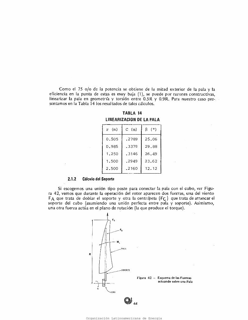
Figura 42 Esquema de las Fuerzas actuando sobre una Pala

R

Si escogemos una unión tipo poste para conectar la pala con el cubo, ver Figu ra 42, vemos que durante la operación del rotor aparecen dos fuerzas, una del viento FA que trata de doblar el soporte y otra la centrrpeta (Fe} que trata de arrancar el soporte del cubo (asumiendo una unión perfecta entre pala y soporte). Asimismo, una otra fuerza actúa en el plano de rotación (la que produce el torque).

2.1.2 Cálculo del Soporte

r (m) e (rn) s (o)

o.sos .2789 25.06 0.98S .3379 29.88 1 .2SO .3146 26.49 1. soo .2949 23.62 2.500 .2160 12. 12

.-····

TABLA 14 UNEARIZACION DE LA PALA

·Corno el 75 o/o de la potencia se obtiene de la mitad exterior de la pala y la eficiencia en la punta de estas es muy baja (1), se puede por razones constructivas, liriearizar la pala en geometrra y torsión entre 0.5 R y 0.9R. Para nuestro caso pre sentamos en la Tabla 14 los resultados de tales cálculos.


45

Este es el mecanismo usado para llevar la potencia desde el rotor hacia la bomba.

2.2 CALCULO DE LA TRANSMISION

ap ~ esfuerzo permisible, kg/cm2

donde:

(2 - 9) d = :.j 1 000 Mi úp

De esta manera se obtiene el diámetro del soporte a través de la expresión:

{2 - 8) Mi = 0,35 Mf + 0,65 V Mf2 + Mt2

Se define el Momento Combinado (Mi) como:

Mf momento de la fuerza aerodinámica, Nm CA = coeficiente de fuerza axial p densidad del aire, kg/m3

Vf velocidad de corte del aire (a esta velocidad el equipo deja de operar), m/seg

A área barrida por el rotor, m2

R radio del rotor, m F e = fuerza centr (peta, N m masa de la pala, kg U velocidad tangencial de la pala a R/2 del centro de giro Mt = contribución de 1 pala al torque total.

Donde:

Mf = CA . + p V f2 • A. R. (2 - 5)

Fe m U2 (2 - 6) (R/2)

Mt Pv (2 7) N.W

Considerando la fuerza del viento aplicada en el extremo de la pala y Ja centrrfu ga a la mitad del radio, tenemos las siguientes cargas:


46

Figura 44 Esquema de Transmisión Directa

(2-11)

Y se cumple:

En este caso, la transmisión será de acuerdo al esquema mostrado en la Figura 44.

ROTOR 1 W , TRANSMISTON 1 WT ~ BOMBA 1 WB ..

Transmisión directa 2.2.1.2 Figura 43 Esquema de Transmisión 1 ndirecta

r' =factor de reducción Donde:

(2-10)

Y se cumple:

w velocidad angular del rotor WE velocidad angular del engranaje Wr velocidad de la transmisión WB velocidad de la bomba

w WE Wr WB JUEGO DE TRANSMISION BOMRA - ENGRANAJES -

Existe una reducción de la velocidad y luego se cambia el movimiento circular en uno alternativo mediante un juego de planetarios, siguiendo el esquema mostrado en Ja Figura 43.

Transmisitin indirecta 2.2.1.1

2.2.1 Tipos de Transmisitin


47

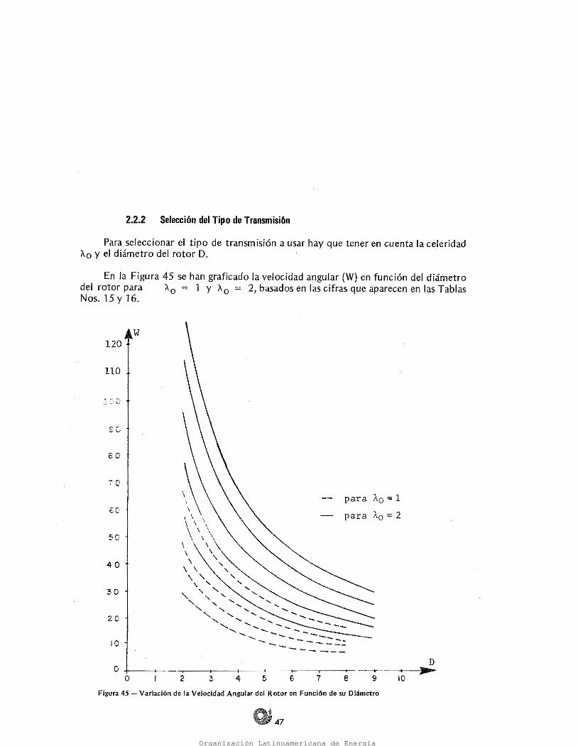
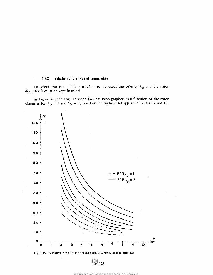
Figura 45 - Variación de la Velocidad Angular del Rotor en Función de su Diámetro

10 9 8 7 6 5 4 2

D ........

para A.o= 1

para A.o= 2

w 120

llO

.~. ·=.'' o

S· e

so ,..., '"

6 C'

50

40

30

20

10

o o

En la Figura 45 se han graficado la velocidad angular (W) en función del diámetro del rotor para A.0 == 1 y A.0 == 2, basados en las cifras que aparecen en las Tablas Nos. 15 y 16.

Para seleccionar el tipo de transmisión a usar hay que tener en cuenta la celeridad A.0 y el diámetro del rotor D.

2.2.2 Selección del Tipo de Transmisión


48

Figura 46 =Vartación de la Celeridad Ao en Función del Diámetro del Rotor y de su RPM

4

D

A.o

2..2

2.0

l. e

f. s

1.4

1. 2

l. o

0.8

0.6

0.4

r ·- ~

r '-

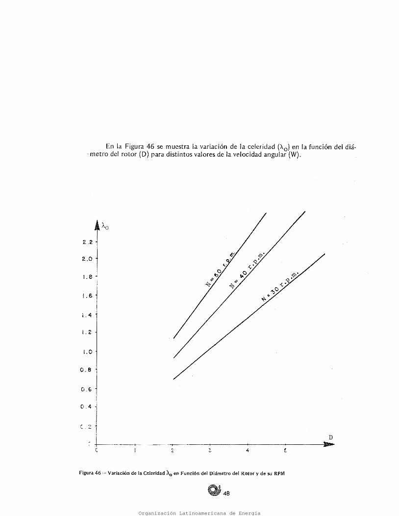
En la Figura 46 se muestra la variación de la celeridad (t,0) en la función del diá- metro del rotor (D) para distintos valores de la velocidad angular (W).


~ 49

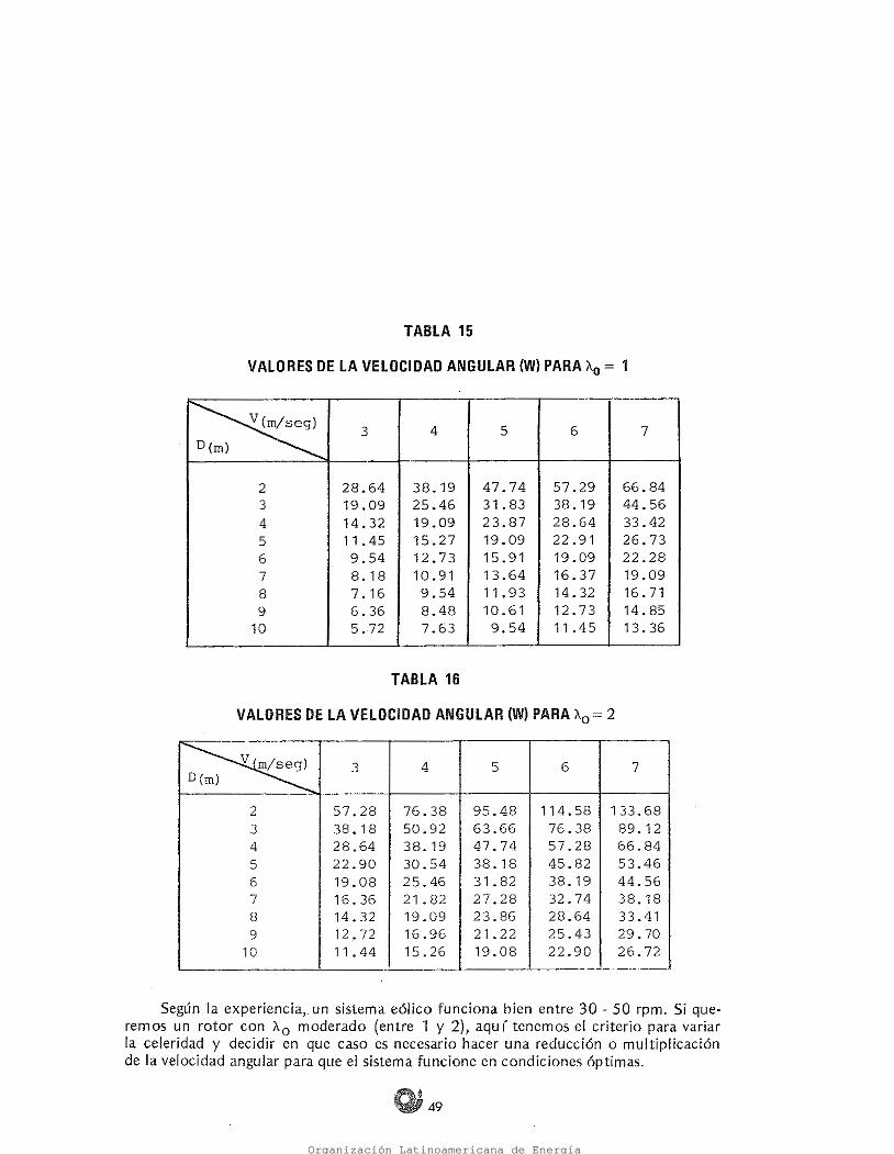
Según la experiencia, un sistema eólico funciona bien entre 30 50 rpm. Si que remos un rotor con A.0 moderado (entre 1 y 2), aqu (tenemos el criterio para variar la celeridad y decidir en que caso es necesario hacer una reducción o multiplicación de la velocidad angular para que el sistema funcione en condiciones óptimas.

~ 3 4 5 6 7

)

2 57.28 76.38 95.48 114. 58 133.68 3 38. 18 50.92 63.66 76.38 89. 12 4 28.64 38. 19 47.74 57.28 66.84 5 22.90 30.54 38. 18 45.82 53.46 6 19.08 25.46 31.82 38. 19 44.56 7 16.36 21.82 27.28 32.74 38. 18 8 14.32 19.09 23.86 28.64 33.41 9 12 .• 72 16.96 21.22 25.43 29.70

10 11. 44 15.26 19.08 22.90 26. 72

TABLA 16

VALORES DE LA VELOCIDAD ANGULAR (W) PARA A0= 2

~ 3 4 5 6 7

)

2 28.64 38. 19 47.74 57.29 66.84 3 19.09 25.46 31. 83 38. 19 44.56 4 14.32 19.09 23.87 28.64 33.42 5 11 . 45 15.27 19.09 22.91 26.73 6 9.54 12.73 15.91 19.09 22.28 7 8. 18 10.91 13.64 16.37 19.09 8 7. 16 9.54 11. 9 3 14.32 16.71 9 6.36 8.48 10.61 12.73 14. 85 10 5.72 7.63 9.54 11. 45 13.36

TABLA 15

VALORES DE LA VELOCIDAD ANGULAR (W) PARA Ao = 1


(2 - 14}

(2 - 15)

P = pw. g. H. Ap. W. f{a)

0 e: o «. g. H. Ap. r. f(a}

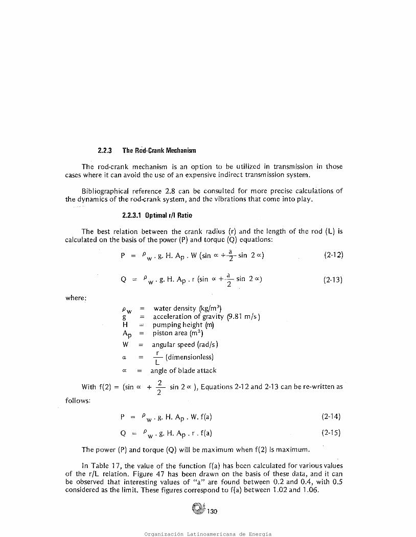
La potencia (P) y el torque (Q) serán máximos cuando f(a) es máxima.

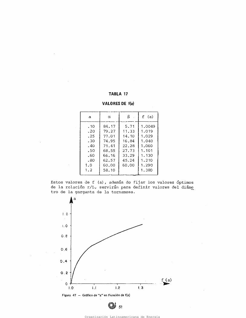
En la Tabla 17 se ha calculado el valor de la función f (a} para diversos valores de la relación r/L. Con estos datos se ha dibujado la Figura 47 en la que se observa que valores interesantes de "a" se encuentran entre 0,2 0,4, considerándose como límite 0,5, lo que corresponde a f (a) entre 1,02 1,06.

Haciendo f (a) ser escritas por:

pw g H Ap w a

= densidad del agua, kg/m3

= aceleración de la gravedad, 9.81 m/seg2

= altura de bombeo, m área del pistón, m2

= velocidad angular, rad/seg = _r_, adimensional

L ángulo de ataque del perfil

== (sen o: + _!____sen 2o: }, las ecuaciones ( 2 12) y 2 13) pueden 2

a:

donde:

(2 - 13) a Q = pw. g. H. Ap· r (sen o:+ T sen 2a:)

( 2 12) a P = ow , g. H. Ap. W (sen o: +2 sen 2o:)

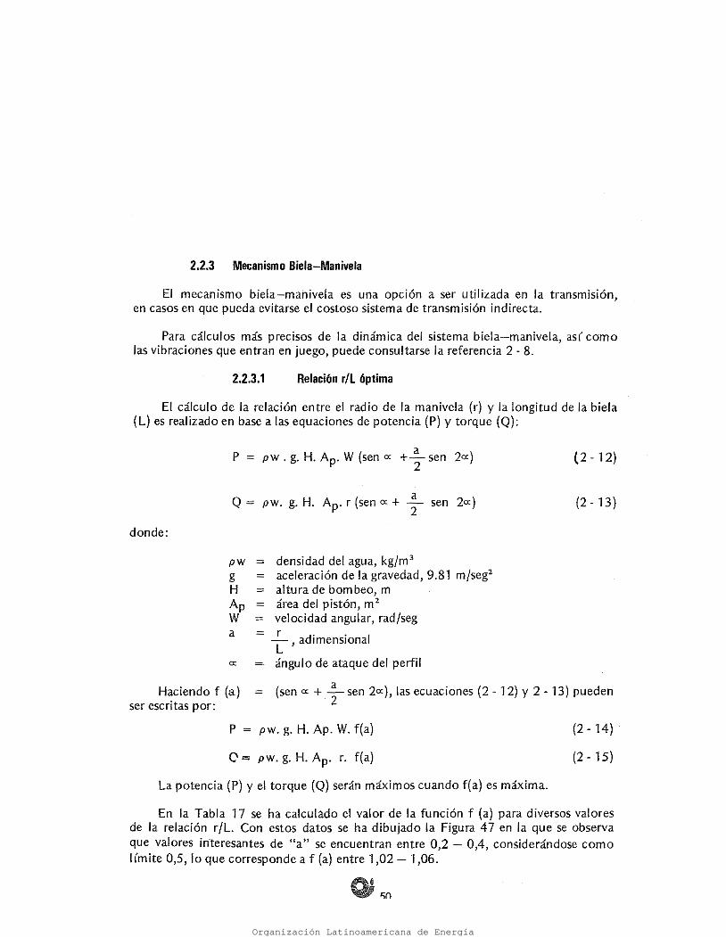
El cálculo de la relación entre el radio de la manivela (r) y la longitud de la biela (L) es realizado en base a las equaciones de potencia (P) y torque (Q):

Relación r/l óptima 2.2.3.1

Para cálculos más precisos de la dinámica del sistema bielamanivela, así como las vibraciones que entran en juego, puede consultarse la referencia 2 8.

El mecanismo bielamanivela es una operen a ser utilizada en la transmisión, en casos en que pueda evitarse el costoso sistema de transmisión indirecta.

2.2.3 Mecanismo Biela-Manivela


51

Figura 47 ·Gráfico de "a" en Función de f(a)

L2

f (a) o ,.._~~~~..--~~~~~~~~-.~~~~~---- l. O l. 3 1.1

0.2

0.4

0.6

0.8

LO

! 2

Estos valores de f (a), además de fijar los valores Óptimos de la relación r/L, servirán para definir valores del diáme tro de la garganta de la tornarnesa.

a

a et s f (a)

. 1 o 84. 17 5.71 1.0049

.20 79.27 11.33 1.o19

.25 77 .01 14. 10 1 .029

.30 74.95 16.84 1. 040

.40 71. 41 22.28 1 .060

.50 68.55 27. 73 1 . 1o1

.60 66. 16 33.29 1. 130

.80 62.57 45.24 1 • 210 1.0 60.00 60.00 1. 290 1. 2 58. 10 1. 380

VALORES DE f(a)

TABLA 17


52

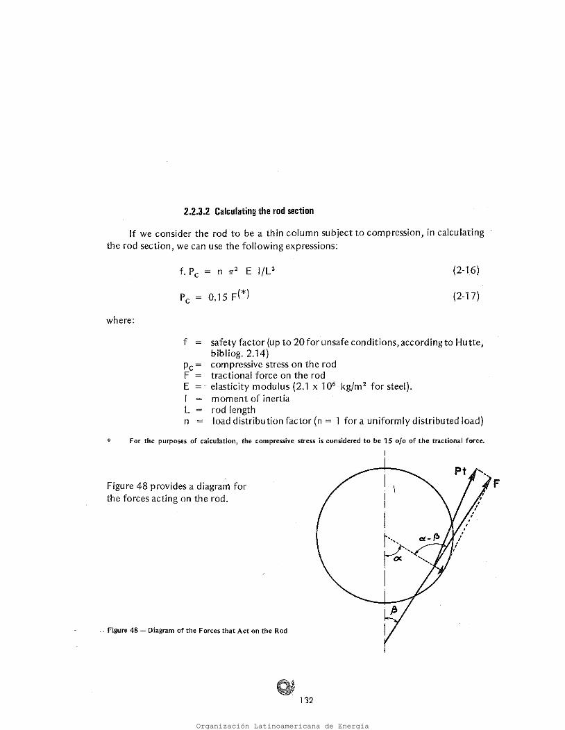
Figura 48 Diagrama de Fuerzas que actúan .sobre la Biela

La Figura 48 muestra el diagrama de fuerzas que actúan sobre la biela. F 1

1

1

~,_

1

(*) para efectos de cálculo se considera la fuerza de compresión como un 15 o/o de la fuerza de tracción.

f factor de seguridad (hasta 20 para condiciones inseguras según Hutte bibliografía 2 14)

Pe = fuerza de compresión sobre la biela F = fuerza de tracción sobre la biela E módulo de elasticidad (2.1 x 106 Kg/m2 para el acero}. 1 = momento de inercia L longitud de la biela n = factor debido a la distribución de la carga (n = 1 para carga uni

formemente distribuida).

donde:

(2 - 16)

(2 - 17)

f'.P¿ = n tr2 E l/L2

Pe ~ 0,15 F(*)

Si consideramos la biela como una columna delgada sometida a compresión pode mos usar, para el cálculo de la sección de ella, las siguientes expresiones:

Cálculo de la sección de fa biela 2.2.3.2


53

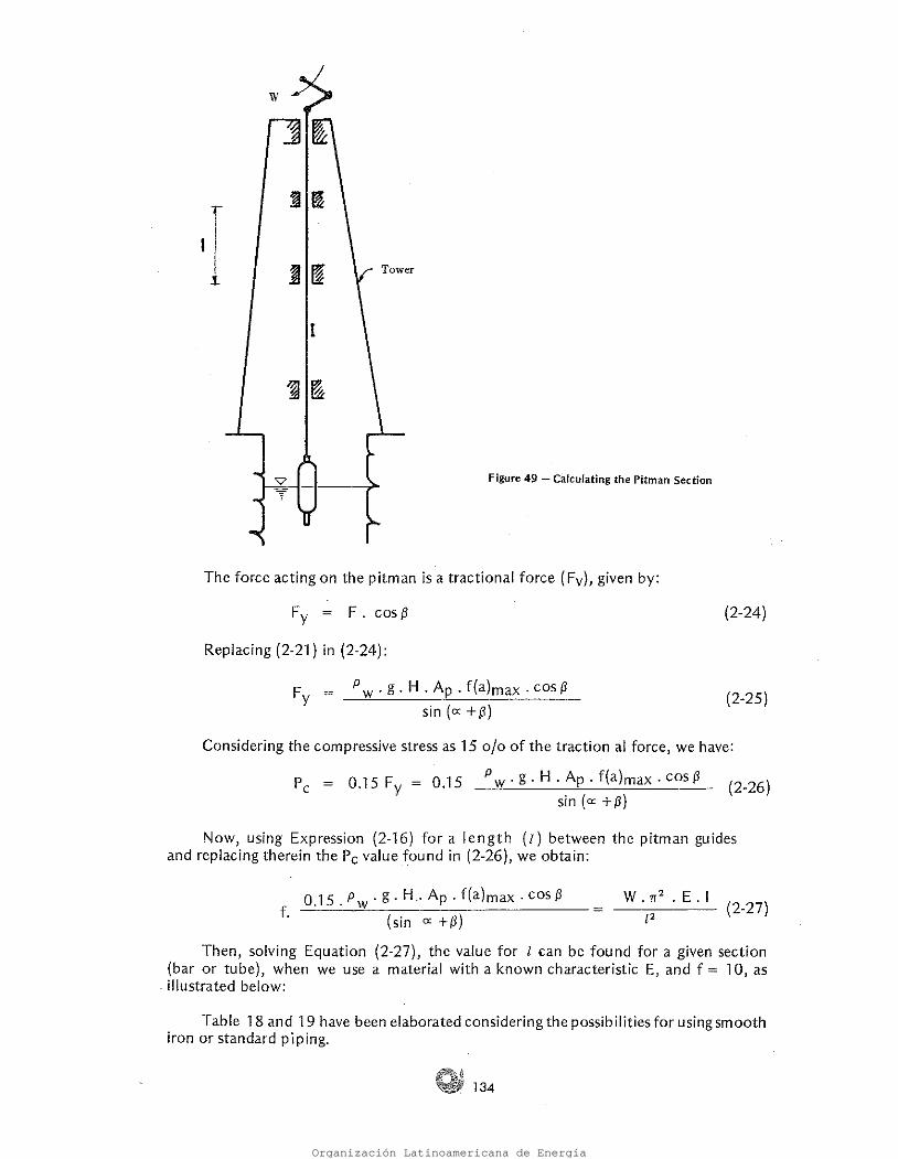
El vástago es un elemento muy esbelto, por lo que es necesario establecer guías intermedias (Ver Figura 49).

Cálculo de la sección del vástago 2.2.3.3

De la expresión (2 23) se obtiene el valor del diámetro L de la biela.

(2 - 23) f 0,15 pw. g. H. Ap. f(a)máx _ n.tr2• E. l. · sen (o: +13) L2

Con el valor de Pe encontrado en la expresión (2 22), volvemos a la expresión (2 16) para calcular la longitud (diámetro) de biela:

{2 22) Pe = 0115. pw. g. H. Ap. f(a)máx sen (o: +13) ·

Ahora, reemplazando (2 21) en (2 17)

(2 21) pw. g. H. Ap. f(a)máx sen (a: +13)

F =

(2 20) Ft = p v«. g. H. Ap. f (a)máx

Luego, sustituyendo (2 20) en 2 19):

y ( 2 19) Ft F = sen (a: tj3)

Sustituyendo (2 15) en (2 18), tenemos:

(2 - 18) Q máx r

TORQUE MAXIMO r

Como se desprende de la Figura 48, F es la componente de Ft que produce el torque máximo, o sea:


~ 54

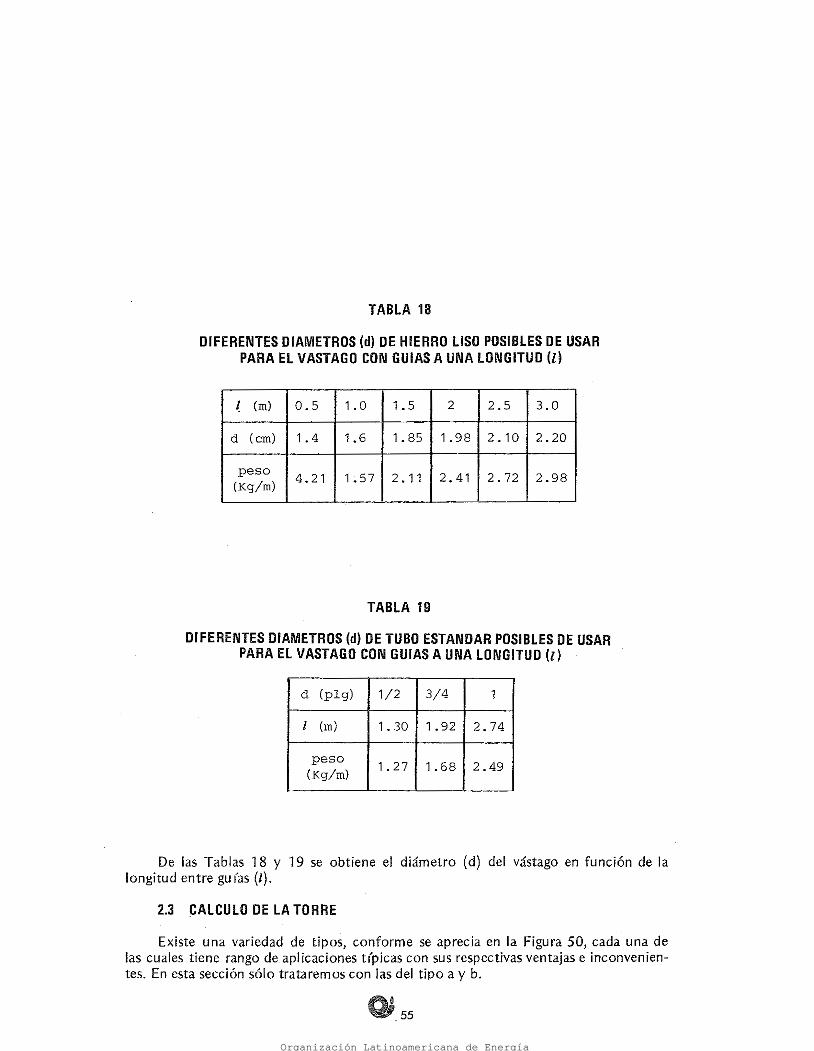
Considerando las posibilidades de usar hierro liso o tubo stándar, se han elabo rado las Tablas Nos. 18 y 19.

Luego, resolviendo la ecuación (2 27) se puede encontrar el valor de 1 para una determinada sección (barra o tubo), cuando usamos un material de característica E conocido y f = 1 O conforme se ilustra a continuación.

(2 - 27) f. O, 15. pw. g. H. Ap. f{a)máx· cos.{3 _ = n. 1T2• E. l.

(sen o: + {3) 1.2

Ahora, usando la expresión (2 - 16) para un longitud (1) entre gu (as del vástago y reemplazando en ella el valor de Pe encontrado en (226), obtenemos:

{2 26) Pe· = O, 15 Fy = O 15 pw. g. H. Ap. f(a)máx· cos {3 ' sen (o: + 13)

·Considerando el esfuerzo de compresión como siendo el 15 o/o del esfuerzo de tracción, tenemos:

(2 - 25) Fy =

(2 - 24) Fy = F. cos {3

Reemplazando (2 21) en(2 24)

pw. g. H. Ap. f(a)máx . cos f3 sen (o: + 13)

La fuerza actuante sobre el vástago es una fuerza de tracción (Fy), dada por:

Figura 49 Cálculo de la Sección del Vástago


~ 55

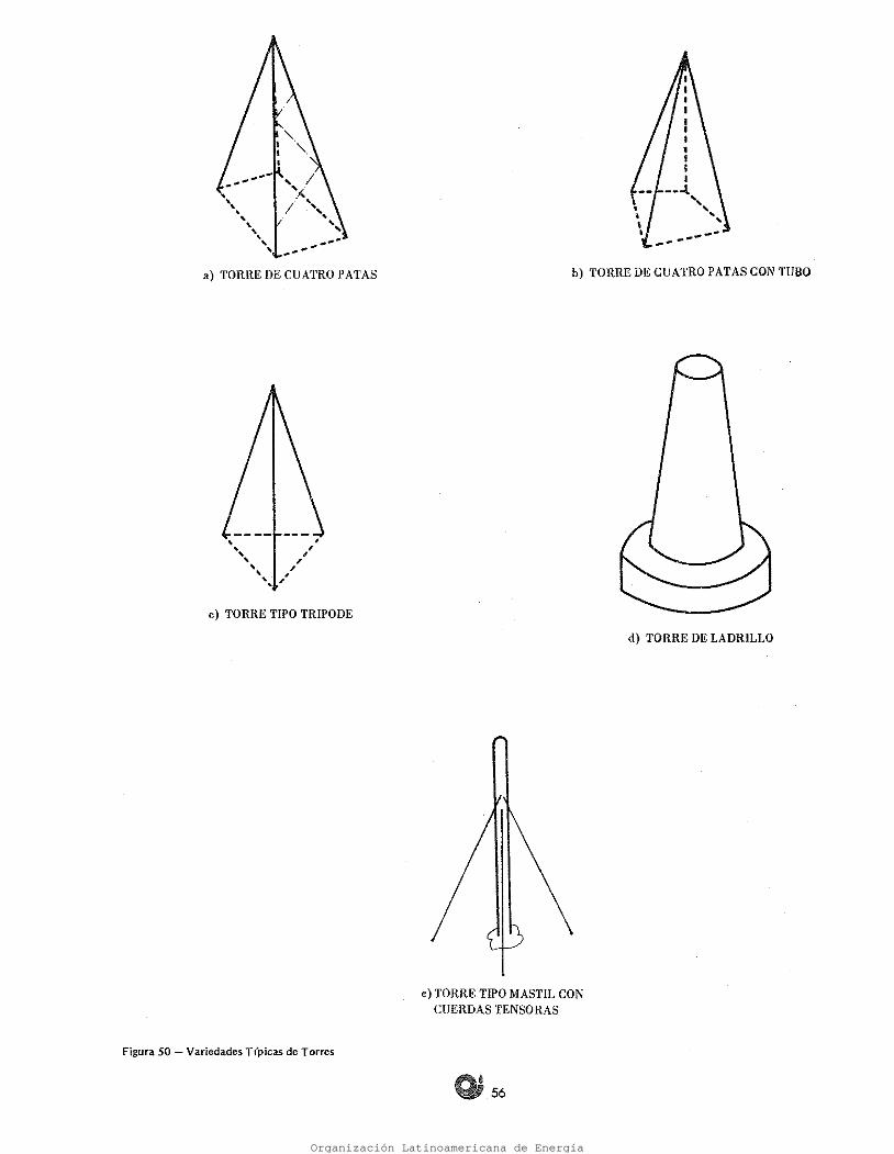
Existe una variedad de tipos, conforme se aprecia en la Figura 50, cada una de las cuales tiene rango de aplicaciones trpicas con sus respectivas ventajas e inconvenien tes. En esta sección sólo trataremos con las del tipo a y b.

2.J CALCULO DE LA TORRE

De las Tablas 18 y 19 se obtiene el diámetro (d) del vástago en función de la longitud entre guías (l).

d (plg) 1/2 3/4 1

J (m) 1. 30 1.92 2.74

peso 1. 27 1.68 2.49 (Kg/m)

TABLA 19

DI FE RENTES DIAMETROS (d) DE TUBO ESTANDAR POSIBLES DE USAR PARA El VASTAGO CON GUIAS A UNA LONGITUD (l)

~ (m) 0.5 1. o 1. 5 2 2.5 3.0

d (cm) 1.4 1.6 1. 85 1.98 2 .10 2.20

peso 4.21 L57 2. 11 2.41 2. 72 2.98 (Kg/m)

TABLA 18

DIFERENTES DIAMETROS (d) DE HIERRO LISO POSIBLES DE USAR PARA El VASTAGO CON GUIAS A UNA LONGITUD (l)


d) TORRE DE LADRILLO

b) TORRE DE CUATRO PATAS CON TUBO

56

e)TORRE TIPO MASTIL CON CUERDAS TENSORAS

Figura SO Variedades Tlpicas de Torres

e) TORRE TIPO TRIPODE

, , , , , , , ' ' ..

' ' ' ...

a) TORRE DE CUATRO PATAS


1 l 1

1 1

1 ho

1

J

(2 - 28}

Figura 51 Variación de la VelÓcidad con la Altura

J

h

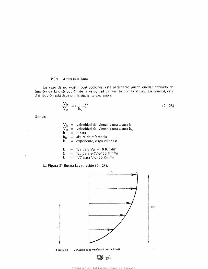
Vo La Figura 51 ilustra la expresión (2 28).

k 1/2 para V0 = 8 Km/hr k = 1 /5 para 8<V 0<56 Km/hr k 117 para V0>56 Km/hr

Vh "" velocidad del viento a una altura h V 0 velocidad del viento a una altura h0 h = altura h¿ altura de referencia k exponente, cuyo valor es: ·

Donde:

vh _ ( h )k Va ho

En caso de no existir obstrucciones, este parámetro puede quedar definido en función de la distribución de la velocidad del viento con la altura. En general, esta distribución está dada por la siguiente expresión:

2.3.1 Altura de la Torre


1

1

1

1

1

1

1

1

1

~

e

6 58

a. Fuerzas en la dirección X: Fx (Vea Figura 53)

2.3.2.1.1 Fuerzas

Figuras 52 Esquema de las Fuerzas Actuantes en la Torre

1

1 MzY

Mx

Tomando como referencia un sistema triortogonal, podernos definir las fuerzas que actúan sobre la torre conforme se ilustra en la Figura 52.

Análisis en condiciones normales 2.3.2.1

2.3.2 Cálculo de la Apertura de las Patas


O) 59

b. Fuerzas en la dirección Y: Fy

fuerza debido a la variación de la velocidad del viento (Ver Figura 54)

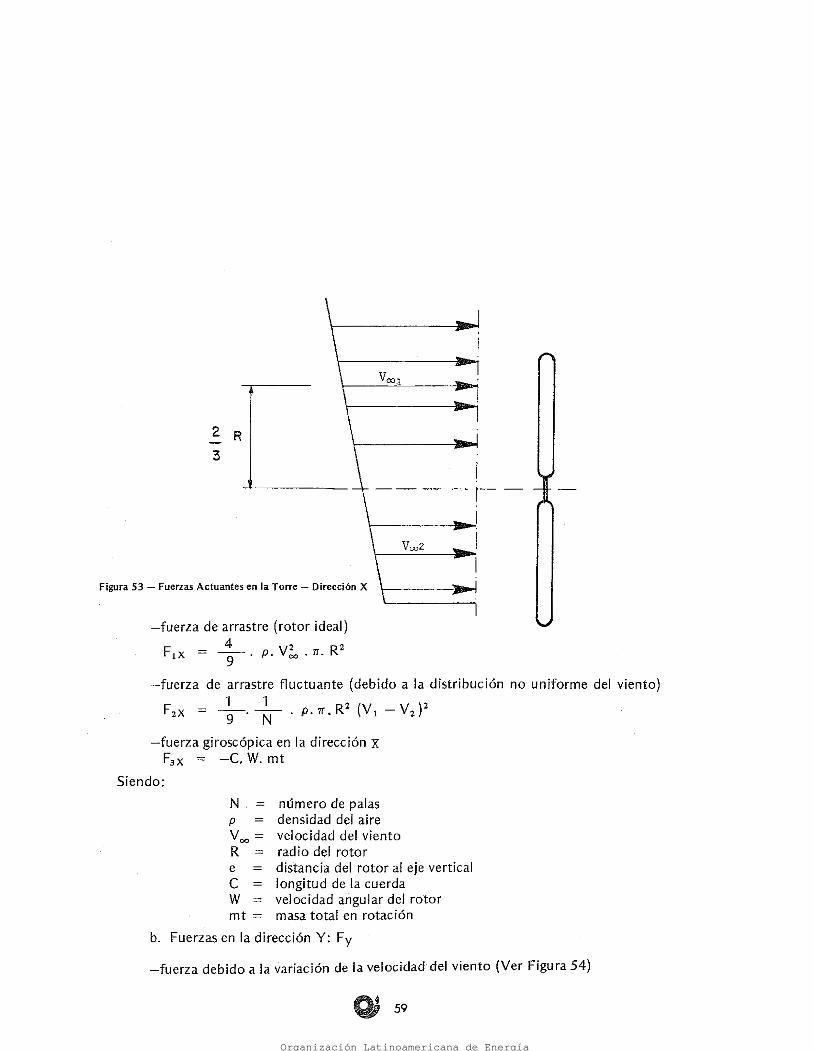
mt=

p voo = R ==

N. número de palas densidad del aire velocidad del viento radio del rotor

e distancia del rotor al eje vertical e longitud de la cuerda w = velocidad angular del rotor

masa total en rotación

fuerza de arrastre (rotor ideal) F 4 y2 Rz ¡X - -9- · p. oo · 7r.

fuerza de arrastre fluctuante (debido a la distribución no uniforme del viento)

F2x = +· +. p.n.R2 (V1 V2)2

fuerza giroscópica en la dirección x F3x = C. W. mt

Siendo:

Figura 53 Fuerzas Actuantes en la Torre Dirección X

1 ¡

2 R 3


Figura SS - Fuerzas Actuantes en la Torre Dirección Y (11)

o; 60

fuerza debido al desbalance del rotor (Vea Figura 55) Faz = ± m,t- er. W2

er = excentricidad del rotor

g = aceleración de la gravedad

=fuerza debido a la masa (m) del rotor F1z=m.g

c. Fuerzas en la dirección Z: Fz

=fuerza debido al desbalance producido por el rotor (Ver Figura 55)

.>

F1Y = Fx. Cos a. Sen a Figura 54 Fuerzas Actuantes en la Torre Dirección Y (1)


61

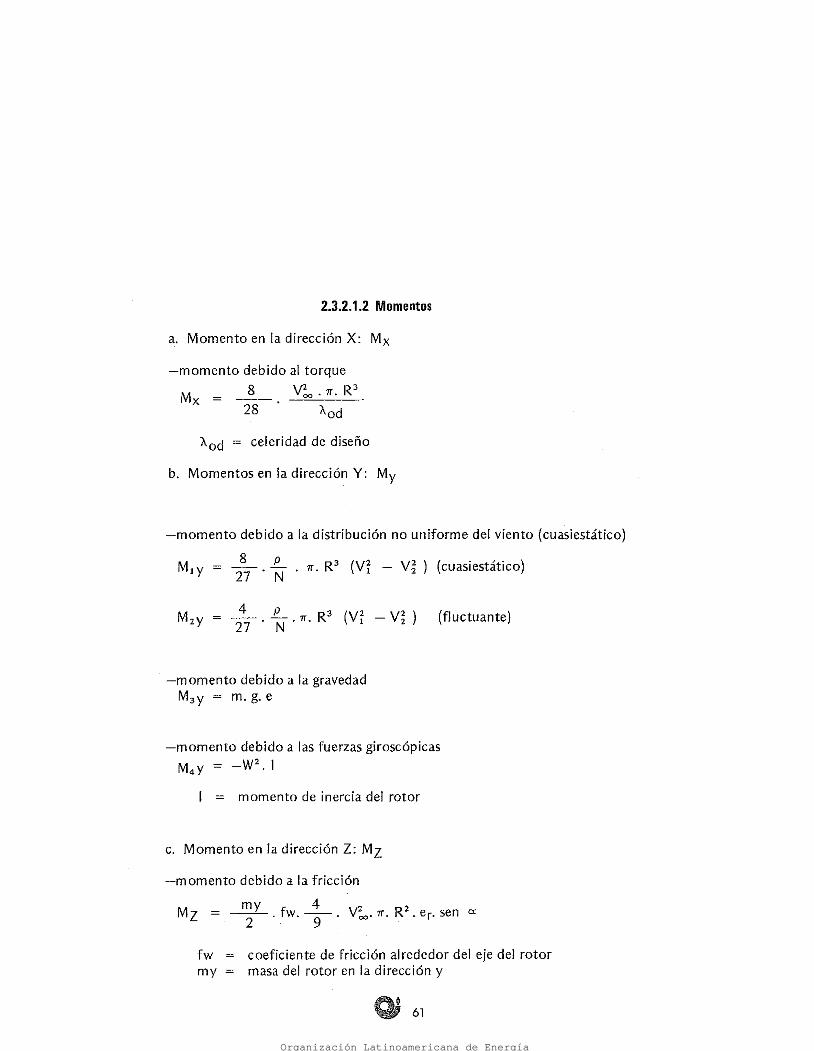
fw coeficiente de fricción alrededor del eje del rotor my masa del rotor en la dirección y

momento debido a la fricción

Mz = _ my fw 4 V2 rr R2 e sen o: 2 · · 9 · oc ' • • r·

c. Momento en la dirección Z: Mz

= momento de inercia del rotor

momento debido a las fuerzas giroscópicas M4y = -W2• 1

momento debido a la gravedad M3y = m. g. e

(fluctuante) 4 P R3 (Vi V~ ) 27· N.1T.

momento debido a la distribución no uniforme del viento (cuasiestático)

M1y = 287

. ~ . tt . R3 (Vi V~) (cuasiestático)

b. Momentos en la dirección Y: My

Aod = celeridad de diseño

momento debido al torque

M X = 8 V2(Xl . n . R 3

28 Aod

a. Momento en la dirección X: Mx

2.3.2.1.2 Momentos


62

V 00 velocidad pico de la zona (huracanes) oc = 30º

b. Condiciones de tormenta (huracanes)

V 00 = la más alta velocidad de trabajo normal ce 30° g 9,8 m/seg2

W 0,5 1 rad/seg p 1,25 Kg/m3

a. Condiciones normales

Criterios para valorar los parámetros 2.3.2.3

c. Momentos (torque)

Mx = ~,6 . _1_. p. V2oo. 1T. R3 X 0 2

1 Mz -< e, ( -2-. p. \1200• ) A prov e. Sen ex: Cos ex:

= área proyectada de Ja torre sobre el plano perpendicular a la di rección del viento.

At proy

b. Fuerza sobre la torre

Ct = coeficiente de presión del viento {Ct ""' 1.6) Aproy = área proyectada del rotor;

1 F x = Ct ( T . P. V2oo ) . Ap roy.

a. Arrastre

Anállsis en condiciones de tormenta 2.3.2.2


8

M X ~

0.4)

63

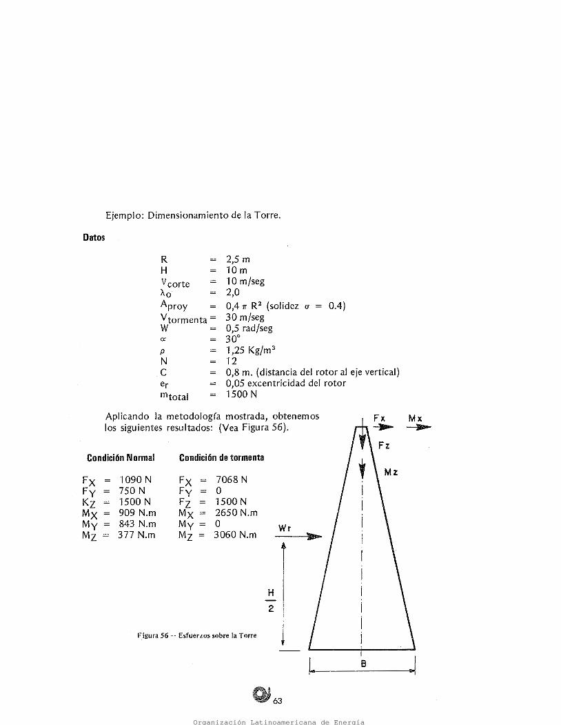
Fígura 56 - Esfuerzos sobre la Torre

H

2

Condición Normal Condición de tormenta

Fx 1090 N Fx 7068 N Fy 750 N Fy = o Kz = 1500 N Fz 1500 N Mx 909 N.m Mx = 2650 N.m My 843 N.m My = o Wr Mz = 377 N.m Mz = 3060 N.rn

Aplicando la metodología mostrada, obtenemos los siguientes resultados: (Vea Figura 56).

p N e er mtotal

V corte A.o Aproy V tormenta= w

R H

Datos

Ejemplo: Dimensionamiento de la Torre.

2,5 m 10 m

= 1 O m/seg 2,0 0,4 rr R2 (solidez u 30 m/seg 0,5 rad/seg 30º 1,25 Kg/m3

12 0,8 m. (distancia del rotor al eje vertical)

= 0,05 excentricidad del rotor 1500 N


64

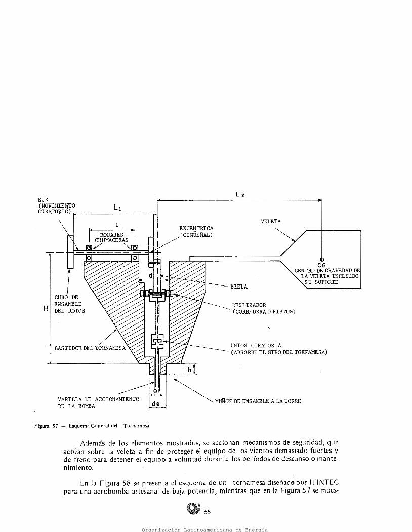
Es el elemento del molino que sirve de eslabón entre el movimrento giratorio del propulsor y el accionamiento alternativo de la bomba; sostiene el rotor y meca nismos de transmisión así como a la veleta.posibilitando la orientación del rotor en la dirección del viento. La Figura 57 muestra los elementos principales de tornamesa.

2.4 CALCULO DEL TORNAMESA

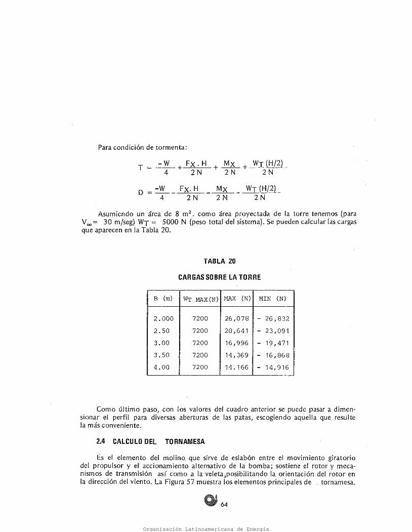
Como último paso, con los valores del cuadro anterior se puede pasar a dimen sionar el perfil para diversas aberturas de las patas, escogiendo aquella que resulte la más conveniente.

B (m} WT MAX(N) JViAX (N) MIN (N)

2.000 7200 26 ,078 26, 832

2.50 7200 20,641 23,091

3.00 7200 16,996 19,471

3.50 7200 14,369 16, 86 8

4.00 7200 14. 166 14,916

CARGASSOBRELATORRE TABLA 20

Asumiendo un área de 8 m2• como área proyectada de la torre tenemos (para V00= 30 m/seg) WT""' 5000 N (peso total del sistema). Se pueden calcular las cargas que aparecen en la Tabla 20.

WT (H/2) 2N

Mx 2N

Fx.H 2N

-w D =-- 4

T = ~ + Fx . H + ~ + WT (H/2) 4 2N 2N 2N

Para condición de tormenta:


65

En la Figura 58 se presenta el esquema de un tornamesa diseñado por ITINTEC para una aerobomba artesanal de baja potencia, mientras que en la Figura 57 se mues

Además de los elementos mostrados, se accionan mecanismos de seguridad, que actúan sobre la veleta a fin de proteger el equipo de los vientos demasiado fuertes y de freno para detener el equipo a voluntad durante los períodos de descanso o mante nimiento.

Figura 57 - Esquema General del Tornamesa

de ~ MUÑON DE ENSl\MBLE A LA TORRE VARILLA DE ACCIONAMIENTO DE LA BOMBA

UNION GIRATORIA (ABSORBE EL GIRO DEL TORNAMESA)

DESLIZADOR (CORREDERA o PISTON)

CG CENTRO DE GRAVEDAD DE

LA VELETA INCLUIDO SU SOPORTE

BIELA

CUBO DE ENSAMBLE H DEL ROTOR

EXCENTRICA (CIGÜEÑAL)

BASTIDOR DEL TORNAMESA

VELETA 1

EJE (MOVIMIE1'TO L1 GIRATO~O),_._~~~~~~~~~


• 66

Así, la longitud L1 mostrada en la Figura 57 debe ser la mínima posible, pero teniendo cuidado que los álabes del propulsor durante su giro no choquen con la estructura de la torre; una vez definida L1 queda definida también la longitud del

Figura 58 - Tornamesa Diseñado) por el ITINTEC/PERU

El dimensionamiento general del tornamesa está relacionado con las caracter(s ticas principales del propulsor, la bomba, la transmisión y la torre.

tra en corte el tornamesa de un molino industrial convencional con reducción de ve locidad por engranajes; en ambos casos puede apreciarse que los elementos principa les se equivalen.


67

PESO DEL ROTOR

~O DE LA TRANSMISION :::::. \ ; ~i'LA COLUMNA DE AGUA

1 1

l PESO DE LA VELETA

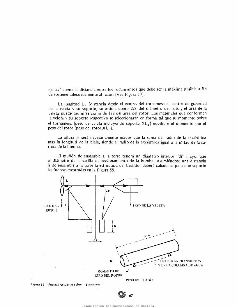
Figura 59 Fuerzas Actuantes sobre Tornamesa

MOMENTO DE GIRO DEL ROTOR

N

• .1 d' I· 1 •

1 !

PESO DEL f H ROTOR

El muñón de ensamble a la torre tendrá un diámetro interior "di" mayor que el diámetro de Ja varilla de accionamiento de la bomba. Asumiéndose una distancia h de ensamble a la torre la estructura del bastidor deberá calcularse para que soporte las fuerzas mostradas en la Figura 59.

La altura H será necesariamente mayor que la suma del radio de la excéntrica más la longitud de la biela; siendo el radio de la excéntrica igual a la mitad de la ca rrera de la bomba.

La longitud L2 (distancia desde el centro del tornamesa al centro de gravedad de la veleta y su soporte) se estima como 2/3 del diámetro del rotor, el área de la veleta puede asumirse como de 1 /8 del área del rotor. Los materiales que conformen la veleta y su soporte respectivo se seleccionarán en forma tal que su momento sobre el tornamesa (peso de veleta incluyendo soporte XL2) equilibre el momento por el peso del rotor (peso del rotor X L1 ).

eje así como la distancia entre los rodamientos que debe ser la máxima posible a fin de sostener adecuadamente al rotor. (Vea Figura 57).


68

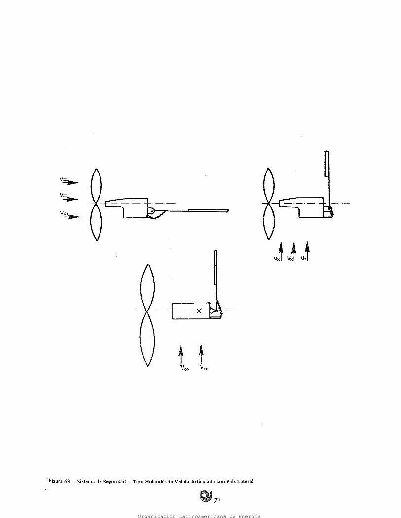
Sistema de rotor de peso variable Plegado manual de la veleta Plegado automático Tipo holandés de veleta articulada con pala lateral.

Existen diferentes tipos; Ver Figuras 60, 61, 62 y 63

2.5.1 Tipos de Sistemas de Seguridad

Por las razones antes mencionadas, se hace necesario bloquear el sistema a la ve locidad de apertura Vf, cuyo valor se puede considerar entre 1 ,5 y 2,5 veces la veloci dad de diseño.

El trabajo del sistema eólico a altas velocidades es peligroso para la bomba, y a su vez produce un trabajo del rotor a condiciones deficientes, produciendo un trabajo deficiente del sistema.

Como se ha visto en acápites anteriores, la turbina eólica se diseña para una velo cidad de viento V 00 la cual deberá trabajar en condiciónes óptimas, a su vez la bom ba se diseña bajo el mismo concepto con el objeto de conseguir un acoplamiento que produzca el mejor rendimiento. Sin embargo, y como se ha visto también, la velocidad del viento es muy variable, pudiendo tener valores muy altos con respecto a V00•

2.5 SISTEMA DE SEGURIDAD


de Peso Variable Tipo Rotor . ma de Seguridad Fig,ra 60 Slste 69


70

Figura 62 Sistema de Seguridad ~Tipo Plegado Automático

V

------

V

------

V _...,...

¡ Flpra 61 Sistema do S•surldad Tipo Plegado Manual de la Veleta

\ -,

\ '"' \ ·"·· \

\

I

/ / / .

/ / . / //

//


JjJ

71

·Figura 63 Sistema de Seguridad Tipo Holandés de Veleta Articulada con Pala Lateral


72

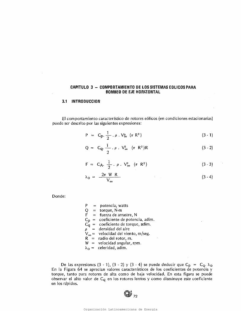
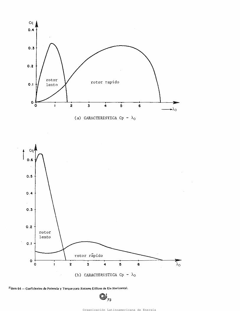
De las expresiones (3 1 ), (3 2) y {3 4) se puede deducir que Cp = Cq. A.0 En la Figura 64 se aprecian valores caracterrsticos de los coeficientes de potencia y torque, tanto para rotores de alta como de baja velocidad. En esta figura se puede observar el alto valor de Cq en los rotores lentos y como disminuye este coeficiente en los rápidos.

P potencia, watts Q torque, N-m F fuerza de arrastre, N Cp coeficiente de potencia, adim. Cq coeficiente de torque, adim. p densidad del aire V 00 = velocidad del viento, m/seg. R = radio del rotor, m. W = velocidad angular, rpm. A.0 = celeridad, adim.

Donde:

(3 - 4) Voo

(3 - 3) F = CA. T p . V200 ( tr R 2 )

2tr W R

(3 - 2)

(3 - 1) P = C l V3 ( R2) P· 2 . P • oo tt

1 Q = Cq. . p . V200 {tr R2) R 2

El comportamiento característico de rotores eólicos (en condiciones estacionarias) puede ser descrito por las siguientes expresiones:

3.1 INTRODUCCION

CAPITULO 3 COMPORTAMIENTO DE LOS SISTEMAS EOLICOS PARA BOMBEO DE EJE HORIZONTAL


73

Figura 64 Coeficientes de Potencia y Torque para Rotores Eólicos de Eie Horizontal.

(b) CARACTERISTICA Cp - Ao 4 6 5 3 2

o -t--~~~....--~-L~~~~-.--~~---.,.--~~-.-~~~-+-~~~~..._~~~ o

rotor rápido

0.1

rotor lento

0.3

0.4

0.5

Cq

(a) CARACTERISTICA Cp - A0 -leo

6 4 3 2

rotor rapido 0.1

0.2

0.3

Cq 0.4

0.2.

t 0.6


74

torque necesario, Nm radio de manivela; m. ángulo que la manivela forma con la vertical altura de bombeo, m diámetro del pistón r/L

Ow r = e :::::

H :::::

dp :::::

a

Donde:

(3 - 5) a ~dp2 = (rsen 8+2sen 28).p. gH. 4 Ow

Para el sistema bielamanivela mostrado, podemos expresar el torque necesario para mantener la manivela a un ángulo 8 con la vertical, mediante la siguiente expre sión:

En dicha figura, una Manivela M de radio r acciona la bomba B, a través de una biela C de longitud L, haciendo recorrer al pistón una carrera S

Fígura 65 - Esquema de Mecanismo para Bombeo

1

En molinos de viento para bombeo, es común el uso de bombas de tipo aspiran teimpelente, las mismas que se ilustran en forma esquemática en la Figura 65.


75

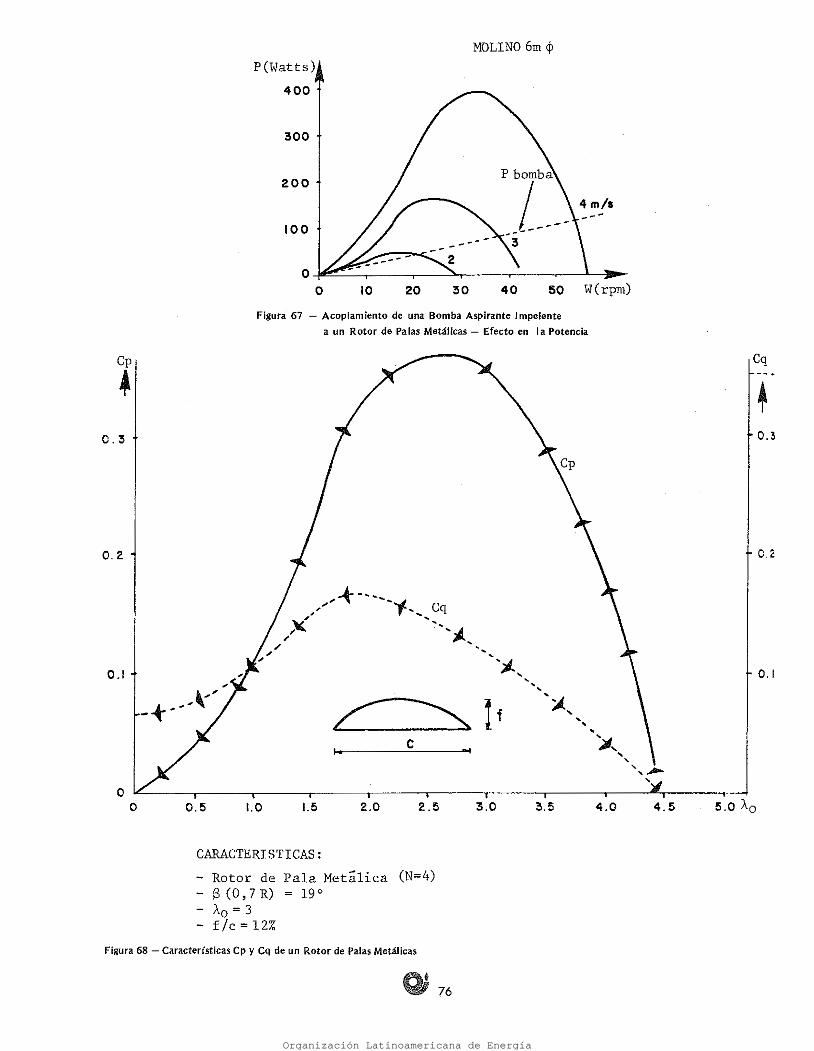
La Figura 67 muestra un rotor de palas metálicas de características Cp p,0') y Cq (A.0) dadas en la Figura 68 , en el cual se ha acoplado una bomba aspirante impelente. Se puede observar que se necesitan vientos de cierta magnitud para poner en operación el sistema y es fácil inducir como cambiaría esta situación si usáramos un rotor lento, con características Cp(A.0) y Cq(t..0) mostradas en la Figura 64.

Para un rotor de características Cp, Cq conocidas, la operación del sistema forma- do cuando se le acopla una bomba aspirante impelente, se puede analizar en condiciones estacionarias si sobre curvas P (w) y Q(w) del rotor se dibujan las correspondientes de la bomba.

Cuando un sistema de bombeo funciona en operación contínua, sólo se manifies- ta el torque promedio OAV = 0MAX/n, pero en el arranque se debe vencer 0MAX·

Figura 66 - Variación del Torque en una Carrera de Trabajo

2n '1T o

Ow

El comportamiento del torque para una carrera de trabajo se representa en forma esquemática en la Figura 66.

Q ~

µ_m_o;:..;x-'-----~-. 1


5.0 A.o

76

Figura 68 Características Cp y Cq de un Rotor de Palas Metálicas

CARACTERISTICAS: - Rotor de Pala Metálica (N=4) - B (O, 7 R) = 19 ° - A.o= 3 f/c = 12%

2.5 1.5 4.0 3.5 4.5 3.0 2.0 l. o

e

Figura 67 Acoplamiento de una Bomba Aspirante Impelente aún Rotor de Palas Metálicas Efecto en la Potencia

20 50 W(rpm) 40 30 10 o

100

0.5 o IL..~~~~~~~~~~~~~~--.-~~---.----~----..---------,--~----.--~--"""-r--------t-~

o

0.1

0.2

0.3

P bomba

/ __ , _ 200

Cq

300

P(Watts) 400

MOLINO 6m <P

0.1

0.2

C.3

Cp

~


77

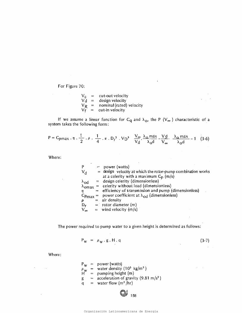
Figura 70 Comportamiento P = f ('{J de un Molino para Bombeo

Voo Vo Ve

1 1 .. 1

p

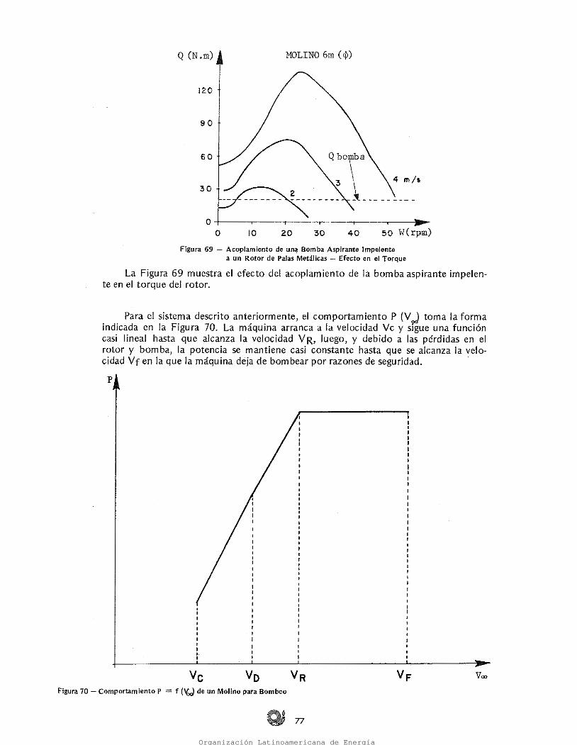
Para el sistema descrito anteriormente, el comportamiento P (V~ toma la forma indicada en la Figura 70. La máquina arranca a la velocidad Ve y sigue una función casi lineal hasta que alcanza la velocidad VR, luego, y debido a las pérdidas en el rotor y bomba, la potencia se mantiene casi constante hasta que se alcanza la velo cidad vr en Ja que la máquina deja de bombear por razones de seguridad.

La Figura 69 muestra el efecto del acoplamiento de la bomba aspirante impelen te en el torque del rotor.

Figura 69 Acoplamiento de una Bomba Aspirante Impelente a un Rotor de Palas Metálicas Efecto en el Torque

50 W(rpm) 40 30 20 10 o

MOLINO 6m ( cj)) Q (N .m)


78

potencia, watts densidad del agua (103 Kg/m3)

altura de bombeo, m = aceleración de la gravedad (9,81 m/seg2 ).

= caudal, m3 /hr.

(3 - 7)

Pw Pw H g q

Donde:

Pw = Pw • g. H. q

La potencia requerida para bombear agua a una altura determinada es:

potencia, watts = velocidad de diseño (velocidad a la cual la combina

ción rotorbomba trabaja a una celeridad con Cp má ximo), m/seg.

= celeridad de diseño, adim celeridad sin carga, adim eficiencia de transmisión y bombeo, adim coeficiente de potencia a "odi adim densidad del aire diámetro del rotor, m velocidad del viento, m/seg.

"od "omáx r¡

CPmáx p

Dr voo

p Vd

Donde:

P e 1 1 D 2. V 3 [ V00 A.0máx Vd ( A.0máx = Pmáx · r¡ · -2 ·p. -4 · n . r · d - . -- -1)] (3 -6) Vd A.0d \IX> A.0d

Si asumimos una función lineal de Cq y A.0 , la característica P (VJ de .un sistema toma la siguiente forma:

velocidad de corte velocidad de diseño velocidad nominal velocidad de apertura

Para la Figura 70:


• 79

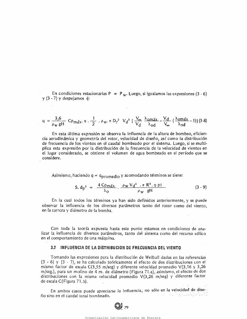
En ambos casos puede apreciarse la influencia, no sólo en la velocidad (le dise ño sino en el caudal total bombeado.

Tomando las expresiones para la distribución de Weibull dadas en las referencias (3 6) y (3 7), se ha calculado teóricamente el efecto de dos distribuciones con el mismo factor de escala C(3,55 rn/seg) y diferente velocidad promedio V(3,16 y 3,26 m/seg.), para un molino de 4 m. de diámetro (Figura 71.a), asimismo, el efecto de dos distribuciones con la misma velocidad promedio V(3,26 m/seg) y diferente factor de escala C(Figura 71. b).

3.2 INFLUENCIA DE LA DISTRIBUCION DE FRECUENCIA DEL VIENTO

Con toda la teor(a expuesta hasta este punto estamos en condiciones de ana lizar la influencia de diversos parámetros, tanto del sistema como del recurso eólico en el comportamiento de una máquina.

En la cual todos los términos ya han sido definidos anteriormente, y se puede observar la influencia de los diversos parámetros tanto del rotor como del viento, en la carrera y diámetro de la bomba.

{3 - 9) Pw V d2 . rr R3. r¡ pt Pw gH

Asimismo, haciendo q = qpromedío y acomodando términos se tiene:

En esta última expresión se observa la influencia de la altura de bombeo, eficien cia aerodinámica y geometr(a del rotor, velocidad de diseño, así como la distribución de frecuencia de los vientos en el caudal bombeado por el sistema. Luego, si se multi plica esta expresión por la distribución de Ja frecuencia de la velocidad de vientos en el lugar considerado, se obtiene el volumen de agua bombeado en el período que se considere.

Cp 1 D 2 V d3 [ Voo Aomáx _Vd ( A.omáx _ 1)] (3_8} máx· 'TI. 2 . Pw. n r Vd Aod Voo A.od

3,6 PwgH

q

En condiciones estacionarias P = P w· Luego, si igualamos las expresiones (3 6) y (3 - 7) y despejamos q:


80

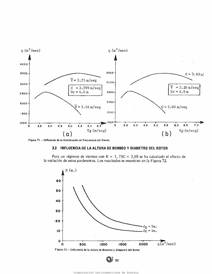
Figura 72 Influencia de la Altura de Bombeo y Diámetro del Rotor

o+--~~~--.~~~~-,--~~~~.--~~~--.~~~~!IP' O 500 1000 1500 2000 q (m3 /mes)

dR = 5m. ~-----dR = 4m. 10

·20

30

40

50

H (m.)

60

Para un régimen de vientos con K = 1, 75C = 3 ,59 se ha calculado el efecto de la variación de estos parámetros. Los resultados se muestran en la Figura 72.

3.3 INFLUENCIA DE LA ALTURA DE BOMBEO Y DIAMETRO DEL ROTOR

( b} Vd (m/seg)

Figura 71 Influencia de la Distribución de Frecuencia del Viento

( a )

IOOO+-~---.~~...-~"""T""~~.--~-.-~--,-~~..-t11..,_1000+-~-.~~.-~--.-~~.---'--.~-..,,--~.-~-..,.---"' ... s s.e 4.0 4.! e.e 5.6 6.0 6_5 a a.s 4.o 4.e s.o 5.!I e.o e.s 1.0

Vd (m/seg)

1500

2000

2500

V = 3.26 m/seg Dr=.4.0m

3000 V= 3,25 m/seg

e =3.599m/seg Dr = 4.0 m

3500

2000

l?!SOO

3000

5500

4000

q (m 3 /mes)


81

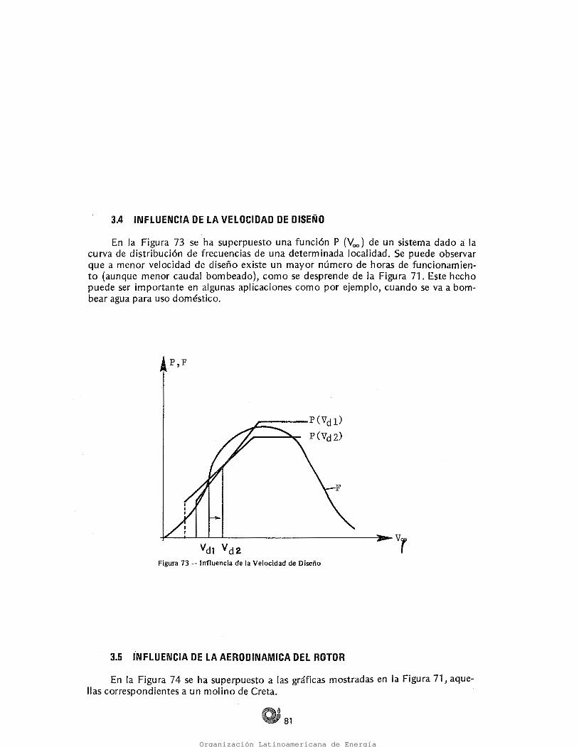
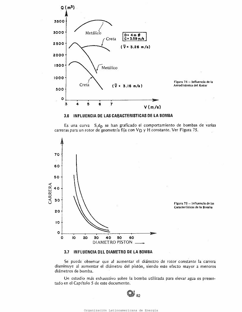
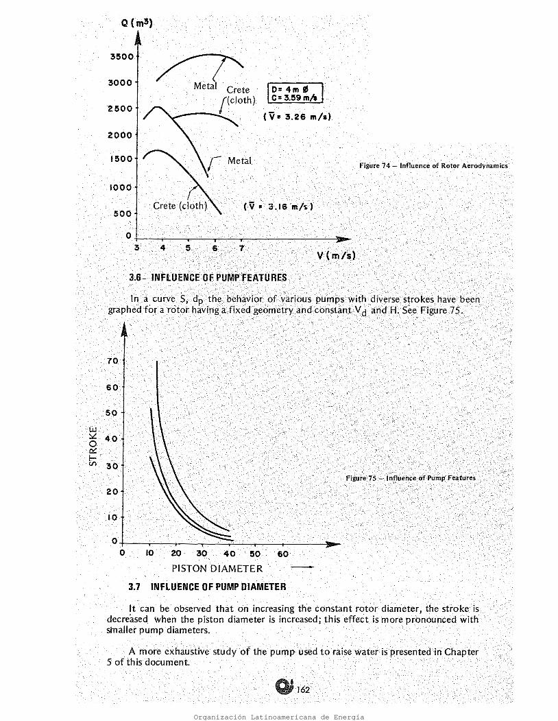
En la Figura 74 se tia superpuesto a las gráficas mostradas en la Figura 71, aque llas correspondientes a un molino de Creta.

3.5 INFLUENCIA DE LA AERODINAMICA DEL ROTOR

Figura 73 Influencia de la Velocidad de Diseño

----P(Vdl) P (Vd 2)

P,F

En la Figura 73 se ha superpuesto una función P (V00) de un sistema dado a la curva de distribución de frecuencias de una determinada localidad. Se puede observar que a menor velocidad de diseño existe un mayor número de horas de funcionamien to (aunque menor caudal bombeado), como se desprende de la Figura 71. Este hecho puede ser importante en algunas aplicaciones como por ejemplo, cuando se va a bom bear agua para uso doméstico.

3.4 INFLUENCIA DE LA VELOCIDAD DE DISEÑO


82

Se puede observar que al aumentar el diámetro de rotor constante la carrera disminuye al aumentar el diámetro del pistón, siendo este efecto mayor a menores diámetros de bomba.

U•1 estudio más exhaustivo sobre la bomba utilizada para elevar agua es presen tado en el Cap(tulo 5 de este documento.

3.7 INFLUENCIA DEL DIAMETRO DE LA BOMBA

20 30 40 50 60 DIAMETRO PISTON -

10 o

<( ~ 40 UJ ~ ~ <( 30 u Figura 75 - Influencia de las

Características de la Bomba

50

60

70

Es una curva S,dp se han graficado el comportamiento de bombas de varias carreras para un rotor de geometría fija con vo y H constante. Ver Figura 75.

V (m/s)

INFLUENCIA DE LAS CASACTERISTICAS DE LA BOMBA

7 6 4

Figura 74 Influencia de la Aerodinámica del Rotor (V=3.16ml•> Creta

O= 4m S C= 3.59 m/l

(V s 3.26 m/1)

r Creta ..:._ 3000

2500

2000

1500

1000

500

o 3

3.6


~ 119

* The density of the air at sea level is more or less 1.23 kg/m3. F or every one thou sand meters of altitude, it is reduced by sorne 10 o/o. Thus, at 4000 meters above sea level, it is 0.8 kg/m3.

lift, N drag, N * air density (specífic gravity) (1.23 kg/m3 )

lift coefficient (dimensionless) · drag coefficient (dimensionless) element area (chord.x differential blade length) wind velocity (m/s)

dl == do p

el= Co = dA = V =

00

Where:

(22)

(2-1) Co.+pV.,;dA

Cl . T p V.,; d A

The components of relative (do) and perpendicular (dL) directions to that of the wind can be expressed by the following mathematical relations:

When the blade of a wind pump is under the effect of an air current.it is put under stress. lf we take one part of the blade, this stress can be broken down into the relative wind direction and the direction perpendicular to that, as shown in Figure 38.

2.1.1 Rotor Geometry

There are different blade arrangements, as can be observed in Figure 37. In this document, we only refer to the type made from a sheet of steel (letter "e" of the figure). However, in bibliographical references 2.5, 2.6, and 2.7, the reader will be able to find information on windmills built with a Cretetype rotor· (letter "a" of the figure), which presents a simple geometry and has interesting technical charac teristics that make it especially attractive for irrigation applications.

2.1 CALCULATING THE ROTOR

CHAPTER 2 - DESIGN OF A HORIZONTAL-AXIS PUMPING SYSTEM

Part 2

I DMILLS FOR PUMPING WATER

The present document is the second of four successive parts.


f) REVERSE SAIL WING

1 1 11

''

1' '1

'· r ; 1 1

e) SAIL CASE

120

e) STEEL PLATE

1. e ~l f

b) RECTANGULAR SAILTYPE

(!t/-------- 1 .. _c_~

d = 0.011 R

o

Figure 37 Sorne Types of Blade Geometry /

d) SAIL WING

f f 1ª .. ====c=.1

CENTER

TIP

~ a) CRETE TYPE

d= 0.011 R

CENTER

TIP


121

Figure 39 Variation in the Optimal Angle for Relative Velocity (</>} with the Tip Speed Ratio ("o)

8 7 6 5 4 3 2 o

20

30

40

number of blades chord length (see Figure 37) (m) drag coefficient {dimensionless) angular speed of the rotor (rpm) design velocity (m/s)

N e = Co = w = Vd=

50

Where: 60 (2-3)

10

By applying the theory of momentum and the equation far energy to the blade element and by integrating along the length of the blade, it can be demonstrated that in order to achieve a maxirnum transformation of the air's kinetic energy into mechanical energy for the blade, the latter should have a torsion that would perrnit 1) an angle </> of the relative wind given in Figure 39 and 2) a chord length that can adjust itself to the function V; (see Figure 40), expressed as follows:

Figure 38 Effect of the Wind on Part of a Blade


122

For the rotor in question, we will consider that curved metal plates, with a section such as that appearing in Figure 41, will be u sed for reasons of construc tion and cost,

From Figure 40 it can be deduced thar the chord length increases up to a certain maximum, near A..o = l, and then dlrninishestowards its end.

In Equation 24, o:= cte is taken for the most minimal (Co/CL) ratio.

(3 blade angle <P = angle of relative velocity o: angle of profile attack

Where:

(2-4) <jJ - o: (3

Frorn Figure 39 it can be deduced that the blade is very open at its base and that this angle diminishes as we approach the tip, since according to Figure 38:

2

3

4

!5

Figure 40 Variation in the Function ¡/¡ with the Tip Speed Ratio (Aal 6


-~ . 123

Ao r (m) <P ( o) B (o) itr e (m)

o. 1 . 125 56.2 52.2 .17715 . 1035 0.2 .250 52.4 48.4 . 31128 • 1819 0.4 .500 45.5 41. 5 . 4 7730 .2789 0.6 .750 39.4 35.4 .54406 .3179 0.8 1 .000 34.5 30.5 .55430 .3239 1.0 1.250 30.5 26.5 .53657 .3135 1.2 1.500 28.0 24.0 .5000 .2922 1. 4 1. 750 23.5 19.5 .4606 . 2688 . 1. 5 1 .875 22.5 18.5 . 45568 . 2663 1.8 2.250 19.0 15.0 .4000 .2337 2.0 2.500 17 .8 13.8 . 38072 .2224

TABLE 13 OPTIMAL BLADE GEOMETRY

Bearing in mind these considerations and doing the calculations indicated in Table 13, we can establish the optimal blade geometry.

The number of blades to be selected as a function of the market availabilities is N = 12, with which a good utilization can be accomplished since the available dimensions are for plates 1.0 x 2.0m.

lf we choose a moderate i\0 value, for example i\0 = 2, for W = 35 rpm, we wíll obtain a (Co/CL) value equal to 0.05.

For the section shown in Figure 41, (Co/CL) = 0.05 and CL = 1.1, for f/c 0.1.

Figure 41 Blade Sectlon To 'Be Dimensioned

f

d


124

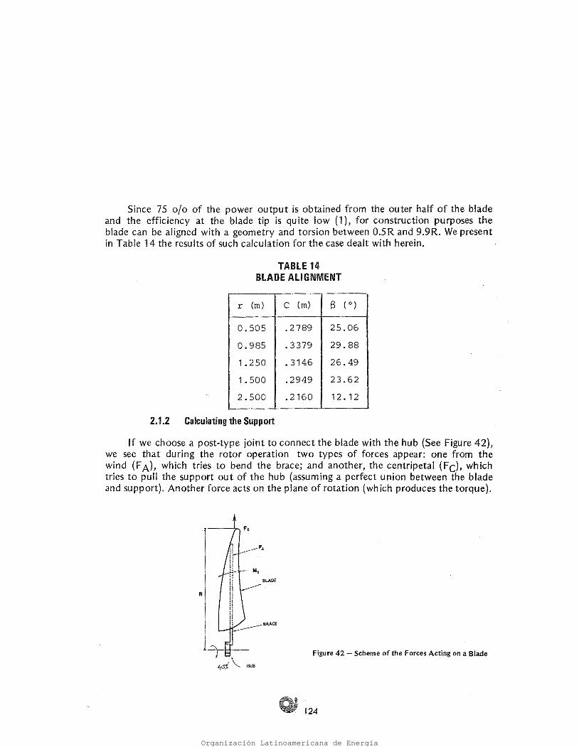
Figure 42 Scheme of the Forces Acting on a Blade

' BL:ADE ¡ »>: , i ' ¡ i

i \ ::::.---- BRACE

LT ·-- '(;;'/. \_ HUB

R

lf we choose a posttype joint to connect the blade with the hub {See Figure 42), we see that durlng the rotor operation two types of forces appear: one from the wind (F AL whlch tries to bend the brace; and another, the centripetal (Fe), which tries to pull the support out of the hub {assuming a perfect union between the blade and support). Another force acts on the plane of rotation (which produces the torque).

2.1.2 Calculating the Support

r (m) e (m) s (o)

0.505 .2789 25.06 0.985 .3379 29. 88 1.250 . 3146 26.49 1.500 .2949 23.62 2.500 .2160 12. 12

TABLE14 BLADE ALIGNMENT

Since 75 o/o of the power output is obtaíned from the outer half of the blade and the efficíency at the blade tip is quite low {1 ), for construction purposes the blade can be aligned with a geometry and torsion between O.SR and 9.9R. We present in Table 14 the results of such calculation far the case dealt with herein.


125

By means of this mechanism,power is carried from the rotor to.the pump.

ªP = permissible stress (kg/cm2)

2.2 CALCULATING tRANSMISSION

(2-9}

where:

Thus, the support diameter is obtained from the following expression:

d = 3j 1000 M¡

ªP

(2-8)

Combined torque (Mi) is defined as follows:

M¡ = 0.35 Mf + 0.65 J Mt2 + Mt2

momentum of the aerodynamic force (Nm) axial force coefficient air density (kg/m3)

cutou tspeed (at this velocity, the equipment ceases to work) (m/s) area swept by the rotor ( m 2)

radius of the rotor( m) centripetal force.(N) blade mass (kg) tangential blade speed, at R/2 from the center of rotation contribution of 1 blade to total torque

Where:

Mt CA = p Vf =

A = R Fe = m = u Mt

Mf = CA . } . p . V f2 • A. R. (2-5)

Fe m U2 (2-6) (R/2)

Mt Pv (2-7) N.W

Considering the force of the wind applied at the blade tip and the centrifuga! force applied to half of the radius, we have the following loads:


126

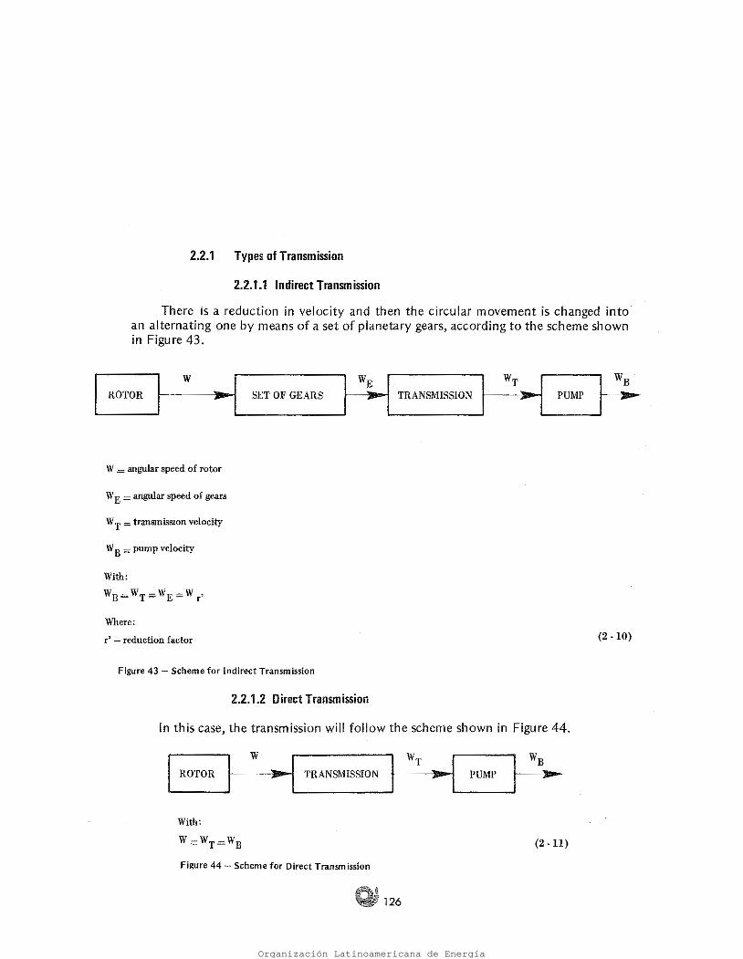
FiJ:ure 44 Scheme for Direct Transm ission

(2. 11)

fw_r_>=~1P_u_M_r _ _:w_B1,.,...,.. W .... , TRANSMISS!ON ROTOR

In this case, the transmission will follow the scherne shown in Figure 44.

2.2.1.2 D irect Transm ission

Figure 43 Scheme for lndirect Transmission

(2. 10) r' reduction factor

Where:

With:

WB=Wr=WE=wr,.

W B ;::;; pump velocity

W T = transmission velocity

W E = angular speed of gears

W = angular speed of rotor

.__R_o_r_o_R__,~-w __ ~.,......,...¡1 SETOFGEARS w· B > W!i... l TRANSMISSION ~T -j PUMF

There is a reduction in velocity and then the circular movement is changed into an alternating one by rneans of a set of planetary gears, according to the scheme shown in Figure 43.

2.2.1.1 lndirect Transmission

2.2.1 Types of Transmission


~ 127

Figure 45 Variation in the Rotor 's Angular Speed as a Function of lts Diameter

6 4 3 9 7 10 e 2

D

\ \ \

\ ' \ ' ' ' '' ', ' ' ...... <, ', ..... , ' ..... .... ' .... ' .................. _

<, ................ ...... ...... ...... ......

- - FOR A = 1 o - FOR/.. = 2 o

w 120

110

100

90

80

70

60

50

40

30

20

10

o o

In Figure 45, the angular speed (W) has been graphed as a function of the rotor diameter for "0 = 1 and "0 = 2, based on the figures that appear in Tables 15 and 16.

To select the type of transmission to be used, the celerity /..0 and the rotor diameter O must be kept in m ind.

2.2.2 Selection of the Type of Transmission


128

Figure 46 Variation in Celerity A.0 as a Function of Rotor Diameter and RPM

A.o

2.2

2.0

1.8

1.6

1.4

l. 2

1.0

0.8

0.6

0.4

0.2

D o >-- o 2 4 5

In Figure 46, the variations in celerity (A.0) are indicated as a function of the rotor diameter (D) far different angular speed values (W).


129

Based on experience, a wind energy system functions well between 30 and 35 rpm. lf we want a rotor with a moderate 1\0 {between 1 and 2), we have the option of varying the celerity and deciding in which case it is necessary to reduce or multiply the angular speed so that the system wíll function under optima! conditions.

~

~I 3 4 5 6 7 !

2 57.28 76.38 95.48 114.58 133.68 3 38. 18 50.92 63.66 76.38 89.12 4 28.64 38. 19 47.74 57.28 66.84 5 22.90 30.54 38. 18 45.82 53.46 6 19 .08 25. 46 31.82 38. 19t 44.56 7 16.36 21. 82 27.28 32.74 38. 18 8 14.32 19.09 23.86 28.64 33.41 9 12. 72 16.96 21.22 25.43 29.70

10 11 . 44 15.26 19.08 22.90 26. 72

TABLE 16 ANGULAR SPEED VALUES (W) (RPM) FOR )1.0 = 2

~ 3 4 5 6 7

)

2 28.64 38. 19 47~74 57.29 66.84 3 19.09 25.46 31. 83 38. 19 44.56 4 14.32 19.09 23.87 28.64 33.42 5 11. 45 15.27 19.09 22.91 26.73 6 9.54 12.73 15. 91 19.09 22.28 7 8. 18 10.91 13.64 16.37 19.09 8 7. 16 9.54 11. 93 14.32 16.71 9 6.36 8. 48 10.61 12. 7 3 14.85

10 5.72 7.63 9.54 11. 45 13. 36

TABLE 15 ANGULAR SPEED VALUES (W) (RPM) FOR )1.0 = 1


t 130

The power (P) and torque (Q) will be maximum when f(2) is maximum.

In Table 17, the value of the function f(a) has been calculated for various values of the r/L relation. Figure 47 has been drawn on the basis of these data, and it can be observed that interesting values of "a" are found between 0.2 and 0.4, with 05 considered as the limit. These figures correspond to f(a) between 1.02 and 1.06.

P = P w : g. H. Ap. W. f(a) (214)

(215) P w . g. H. Ap . r . f(a) Q

follows:

a f (dimensionless)

o:: angle of blade attack

With f(2) = (sin ex: + 2 sin 2 <). Equations 2-12 and 2-13 can be rewritten as 2

water density (kg/m3)

acceleration of gravity (9.81 m/s) purnping height (m) pistan area (m2)

angular speed (rad/s)

Pw g H = Ap w

where:

(2-13) Q = P HA ·(· +ª . 2) W . g. . p . r Sin o:: l Sin o::

(212} P = P w. g. H. Ap. W (sin ex: +-T sin 2 =)

The best relation between the crank radius (r) and the length of the rod (L) is calculated on the basis of the power (P) and torque (Q) equations:

2.2.J.1 Optima! r/l Ratio

Bibliographical reference 2.8 can be consulted for more precise calculations of the dynamics of the rod-crank system, and the vibrations that come into play.

The rodcrank mechanism is an option to be utilized in transmission in those cases where it can avoid the use of an expensive indirect transmission system.

2.2.3 The Rod-Crank Mechanism


131

Figure 47 Graph of "a" as a Function of f(a)

f (a) 1.2 l. 3

1.2

l. o

o.a

0.6

0.4

0.2

o 1.0 1.1

These values for f(a), in addition to setting the optima! values for the r/L relation, will serve to define diameter values for the turntable throat.

o

a a s f (a)

. 10 84. 17 5.71 1. 0049

.20 79.27 11 . 33 1. o 19

.25 77 .01 14. 10 1. 029

. 30 74.95 16.84 1. 040

.40 71. 41 22.28 1. 060

.so 68.55 .· 27. 73 1. 1o1

.60 66. 16 33.29 1. 130

.80 62.57 45. 24 1.210 1.0 60.00 60.00 1. 290 1. 2 58. 1 o 1. 380

TABLE 17 VALUES FOR f(a)


1'32

. . Figure 48 Diagram of the Forces that Act on the Rod

F Figure 48 provides a diagram for the forces acting on the rod .

* For the purposes of calculation, the compressive stress is considered to be 15 o/o of the tractional force.

f = safety factor (up to 20forunsafe conditions,accordingto Hutte, bibliog. 2.14)

Pe= compressive stress on the rod F tractional force on the rod E = elasticity modulus (2.1 x 106 kg/m2 for steel). 1 = moment of inertia L = rod length n = load distribution factor (n = 1 for a uniformly distributed load)

where:

(2-17)

(216) f.P¿ = n 71'2 E l/L2

lf we consider the rod to be a thin column subject to compression, in calculating the rod section, we can use the following expressíons:

2.2.3.2 Calculating the rod section


~ 133

The pitman is a very thin element, for which reason it is necessary to establish intermediate guides. (See Figure 49). ,

2.2.3.3 Calculating the pitman section

The value for the rod diameter L can be obtained from the foregoing expression.

(2-23) n . 1T 2 • E. l.

L2 f. 0.15pw.g.H.Ap.f(a)max

sin (ex: +/3)

With the value of Pe found in Expression (222), we go back to Equation (216) to calculate the length (diameter) of the rod:

(~-22) P w . g . H . Ap . f(a)max

sin ( ce+ /3) Pe == 0.15.

Now, replacing (22l) in (217):

(221) Pw. g. H. Ap. f(a)max sin (a::+f3)

F ==

Then, substituting (220) in (219):

(220) Ft == "«: g. H. Ap. f(a)max

sin (a::+f3)

Substituting Equation (215) in (218), we have:

(2-19) F == and

(218) Qmax r

MAXIMU_ryt TORQUE r

As can be ascertained from Figure 48, F is the component of Ft that produces the maximum torque, in other words:


134

Table 18 and 19 have been elaborated considering the possibillties for using smooth iron or standard p iping.

Then, solving Equation (227), the value for l can be found for a given section {bar or tube), when we use a material with a known characteristic E, and f = 1 O, as illustrated below:

(227} W. rr2 • E . 1

l2

0.15. Pw. g. H .. Ap. f(a)max. cos/3 f. (sin a: +{3)

Now, using Expression (216) for a length (!) between the pitman guides and replacing therein the Pe value found in (226), we obtain:

(226) P w . g . H . Ap . f(a)max . cos {3

sin (a: + JJ} Pe = 0.15 Fy = 0.15

Considering the cornpressive stress as 15 o/o of the traction al force, we have:

(2-25} P w . g. H . Ap . f{a)max . cos J)

sin (a: +M

(224) Fy = F. cos J)

Replacing {221) in (224);

The force acting on the pitman is a tractional force (Fv), given by:

Figure 49 Calculatlng the Pitman Section


135

As can be appreciated from Figure 50, there are a variety of types of towers, each one of which has a range of typical applications, as a function of their respective advantages and disadvantages. In this section, we will only deal with types "a" and "b,,

2.3 CALCULATING THE TOWER

From Tables 18 and 191 the pitman diarneter (d) can be obtained as a function of the length between gu ides ( l ).

d (in) 1/2 3/4 1

t (m) 1. 30 1. 92 2.74

weight 1. 27 1.68 2.49 (kg/m) ..

TABLE 19 DIFFERENT DIAMETERS (d) OF STANDARD PIPING APT FOR USE

IN A PITMANWITH GUIOES HAVING A LENGTH l

l (m) 0.5 1.0 1. 5 2 2.5 3.0

d (cm) 1 . 4 1.6 1. 85 1. 98 2. 1 o 2.20

weight 4.21 1 . 5 7 2. 11 2. 41 2. 72 2.98 (kg/m)

TABLE 18 DIFFERENT DIAMETERS (d) OF SMOOTH STEEL APT FOR USE IN A PITMAN

WITH GUIDES HAVING A LENGTH t


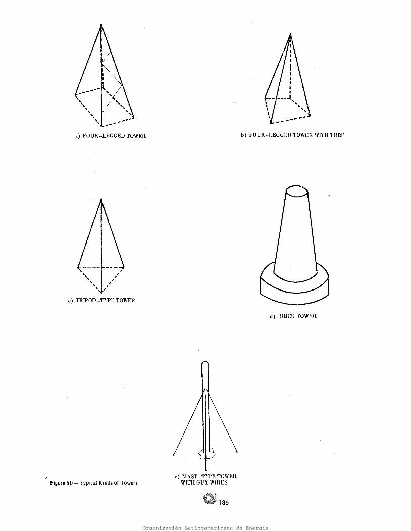
d) BRICK TOWER

h) FOURLEGGED TOWER WITH TUBE

136

e) MASTTYPE TOWER WITH GUY W1RES Figure 50 Typical Kinds of Towers

e) TRIPODTYPE TOWER

' , ', ,~ ' , ' , ' , '• ,

a) FOURLEGGED TOWER


(228)

~ 137

Figure 51 Variations in Speed as a function of Height

J

h

Yo

Figure 51 illustrates Expression (228).

Vh ::; wind velocity ata height h V 0 = wind velocity ata height h0 h height h0 = reference height k = exponent, whose value is:

k = 1/2 for vo = km/br k = 1/5 for 8.< V0< 56 km/hr k = 1 /7 for V 0 > 56 km/hr

Where:

k h ho

=

When no obstructions exist, this test can de defined as a function of the wínd velocity distribution with height. In general, this distribution is given by the following expression:

2.3.1 Tower Height


1

1

1

1

1

1

1

1

1

1 ¡

e

138

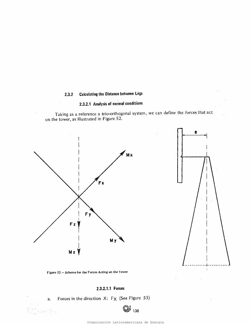
a. Forces in the direction X: Fx (See Figure 53)

2.3.2.1.1 Forces

Figure 52 Scheme for the Forces Acting on the Tower

1

1 MzY

M x

./

Taking as a reference a trioorthogonal system, we can define the forces that act on the tower, as illustrated in Figure 52.

2.3.2.1 Analysis of normal conditions

2.3.2 Calculating the Distance between Legs


139

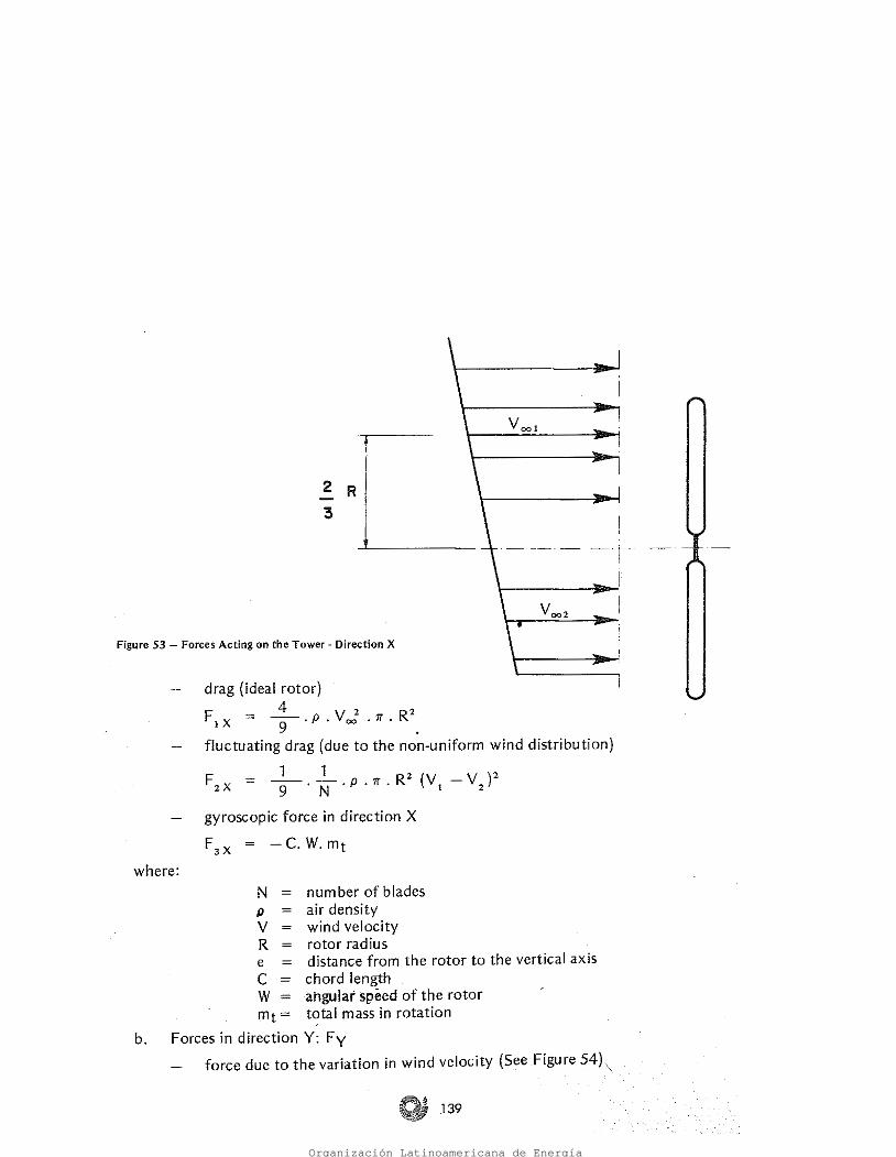
N nurnber of blades p air density V wind velocity R rotor radius e distance from the rotor to the vertical axis e chord length W = angular speed of the rotor mt = total mass in rotation

b. Forces in direction Y: Fy force dueto the variation in wind velocity (See.Figure 54)',

where:

gyroscopic force in direction X

F3X = C.W.mt

. fluctuating drag (dueto the nonuniform wind distribution)

F z x = +-. ~. P • 1r • R2 (Vi V z )2

drag (ideal rotor)

F 4 V 2 R2 1X = g.p. oo .tr.

Figure 53 Forces Acting on the Tower Dírectíon X

2

3


Figure 55 - Forces Ac:ting on the Tower · Directíon Y (11)

.140

(ere:: rotor eccentricity)

forces dueto rotor imbalance (see Figure 55). Faz = ± m t . e r . w2 .

(g = acceleration of gravity)

forces dueto the rotor rnass (rn) F1z = m.g

c. Forces from direction Z: Fz

force dueto the imbalance produced by the rotor (See Figure 55)

/ F1y = Fx cosa. sin a

Figure 54 Forces Acting on the Tower · Directien Y (1)


141

\

f w = friction coefficient far around the rotor axis my = rotor mass in direction y

Mz = T. fw. : . V~. tt : R2• er.· sin°'

momentum dueto friction

c. Momentum in direction Z: Mz

M = -W2 1 4 y .

1 = momentum dueto rotor inertia

momentum dueto gyroscopic forces

momentum due to gravity

M3 y = m. g. e

Ml y i7 . ~ . tt , R3 (VI 2 - v2 2) (quasi-static)

M 4 P R3 (V1 2 V2 2) (fluctuating) .2Y n·N.n.

momentum dueto the non-uniform wind distribution non-uniform

b. Momentum in direction Y: My

V~ . n . R3

Aod

Aod = design celerity

momentum dueto torque

a. Momentum in direction X: M X

2.3.2.1.2 Momentum


142

V oo peak speed in the zone (hurricanes) ce = 30°

·· b. Storm conditions (hurricanes)

V""'_= the h ighest normal working speed ce 30º , g 9.8 m/s2

W = 0.5 - rad/s p = 1 .25 kg/m3

a. Normal conditions

2.3.2.3 Criteria for assessing parameters

Mz ~ Ct ( T. p. V~ ) A .proj : e. sin ex: Cos ce

= 0~6 . _1 _. P ~y~ . 1r • R3 A 0 2 Mx

Momentum (torque) c.

At proj = · projected tower area on the plane perpendicular to. the wind direction

F w e, ( + p V~ ) At pro j·

Ct wind pressure coefficient (Ct = 1.6) Aproj = projected rotor area

b. Stress on the tower

a. Drag

2.3.2.2 Analysis of stress under storm conditions


ó 143

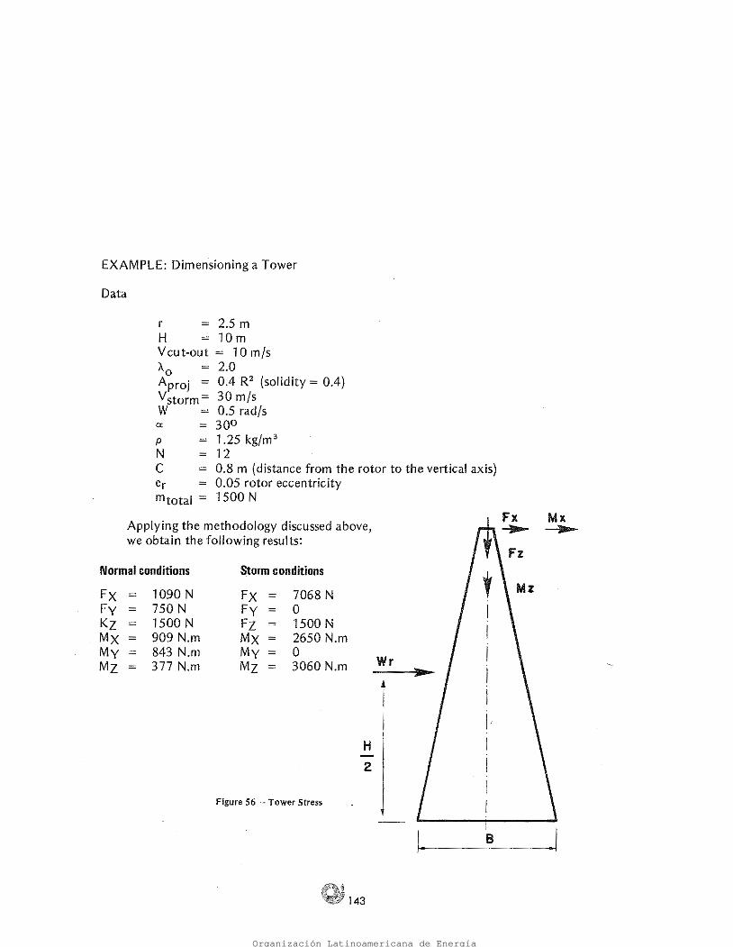
figure 56 - Tower Stress

H 2

Applying the methodology discussed above, Mx

----- we obtain the following results:

Normal conditions Storm conditions

Fx = 1090 N Fx 7068 N Fy = 750 N Fy o Kz = 1500 N Fz 1500 N Mx 909 N.m Mx 2650 N.m My = 843 N.m My o Mz = 377 N.m Mz 3060 N.m Wr ..

r = 2.5 m H = 10m Vcutout = 10 m/s A.0 2.0 Aproj = 0.4 R2 (solidity = 0.4) Ystorm= 30 m/s W = 0.5 rad/s a: :;:: 30º p = 1.25 kg/m3

N 12 C = 0.8 m {distance from the rotor to the vertical axis) er = 0.05 rotor eccentricity mtotal = 1500 N

Data

EXAMPLE: Dimensioning a Tower


¡¡ 144

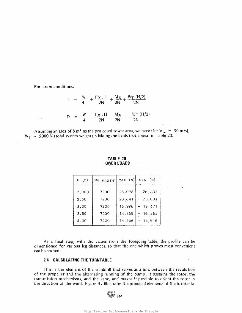
This is the element of the windmill that serves as a link between the revolution · of the propeller and the alternating running of the pump; it sustains the rotor, the transmission mechanisms, and the vane, and makes it possible to orient the rotor in the direction of the wind. Figure 57 íllustrates the principal elements of the turntable.

2.4 CALCULATING THE TURNTABLE

As a final step, with the values from the foregoing table, the profile can be dimensioned for various leg distances, so that the one which proves most convenient can be chosen.

B (m) WT MAX(N) MAX (N) MIN (N)

2.000 7200 26,078 - 26,832 2.50 7200 20,.641 - 23,091 3.00 7200 16,996 19,471 3.50 7200 14,369 16,868 4.00 7200 14. 166 14,916

TABLE 20 TOWER lOADS

Assurn ing an a rea of 8 m 2 as the projected tower area, we have (for V 00 = 30 m/s), WT = 5000 N (total system weight), yieldingthe loads that appear in Table 20.

For storm conditions:

T w + Fx. H + Mx + WT (H/2) 4 2N 2N 2N

D w Fx. H -~X __ WT (H/2) 4 2N 2N 2N


145

Figure 58 presents the scherne for a turntable designed by ITINTEC for a hand made wind pump with a low power capacity, while Figure 57 shows a crosssection

In addition to the elements shown, safety mechanisms are activated to act on the vane in order to protect the equipment from overly strong winds and to brake the equipment at will for periods of rest and maintenance.

CG CENTER OF GRAVITY OF

WINDVANE INCLUDING BRACE

de

Figure 57 General Scheme for the Turntable

PUMP'S DRIVING ROD

ROTATING JOINT (ABSORBS ROTATION

OFTURNTABLE)

'fUltNTABLE FRAME

ASSEMBLY SLll'WAY (RUNNER OR PISTON)

HUBOFROTOR

VANE 1 H

Li

WINDVANE ·i AX1S(ROTATING

MOVEMENT)


~ 146

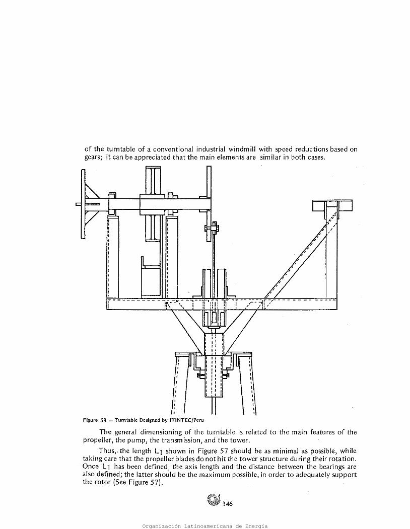
Figure 58 - Turntable Designed by ITINTEC/Peru

The general dimensioning of the turntable is related to the main features of the propeller, the purnp, the transmission, and the tower.

Thus,. the length L l shown in Figure 57 should be as minimal as possible, while taking care that the propeller blades do not hit the tower structure du ring their rotation. Once L 1 has been defined, the axis length and the distance between the bearings are also defined; the latter should be the maxirnum possible, in order to adequately support the rotor (See Figure 57}.

of the turntable of a conventional industrial windmill with speed reductions based on gears; it can be appreciated that the main elements are similar in both cases.


147

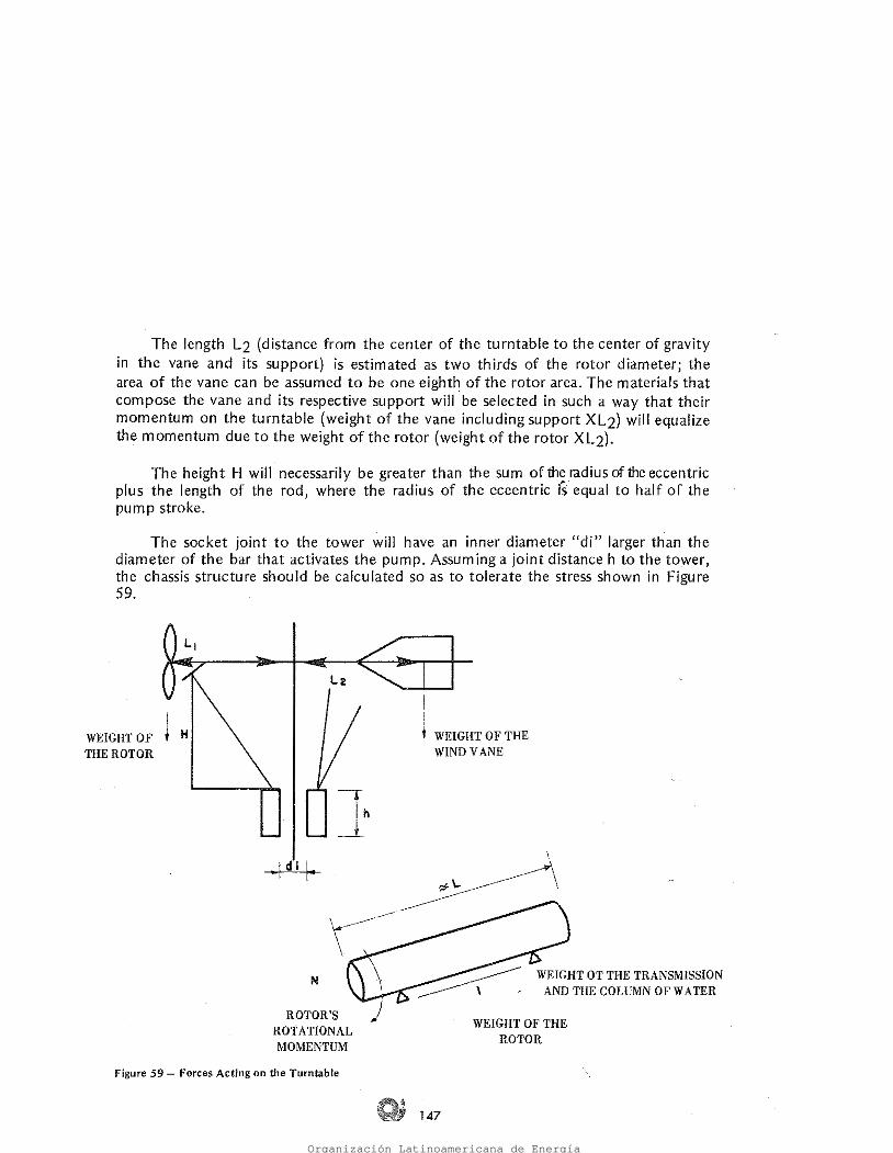
Figure 59 Forces Acting on the Turntable

WEIGHT OF THE ROTOR

~ WEIGHT OT THE TRANSMISSION ~ \ AND THE COLUMN OF WATER

N

ROTOR'S ROTATIONAL MOMENTUM

.. ¡di ¡ ..

WEIGHT OF THE WlND VANE

L2

WEIGHT OF THEROTOR

The socket joint to the tower will have an inner diameter "di" larger than the diameter of the bar that activates the pum p. Assuming a joint distance h to the tower, the chassis structure should be calculated so as to tolerate the stress shown in Figure 59.

The height H will necessarily be greater than the sum ofthe radius of theeccentric plus the length of the rod, where the radius of the eceentric is equal to half of the pump stroke.

The length L2 (distance from the center of the turntable to the center of gravity in the vane and its support) is estimated as two thirds of the rotor diameter; the area of the vane can be assumed to be one eighth of the rotor area. The materials that compase the vane and its respective support will be selected in such a way that their momentum on the turntable (weight of the vane including support XL2) will equalize the momentum dueto the weight of the rotor (weight of the rotor XL2).


148

Rotor system with variable weight Manual vane bending Autornatic vane bending Dutchtype vane designed with a lateral blade.

There exist different types, as illustrated in Figures 60, 61, 62, and 63:

2.5.1 Types of Safety Systems

For the aforementioned reasons, it becomes necessary to block the system at the cutout speed Vf, whose value can be considered between 1.5 and 2.5 times the design velocitv.

A wind energy system working at high speeds is dangerous for the pump and also makes the rotor work under poor conditions, thereby producing poor system output.

As has been seen in previous headings, the wind turbine is designed for a wind velocity V oo , where it should work under optimum conditions, while the purnp is de· signed with the same concept in mind, in orderto obtain the coupling that will produce the best yield. Nevertheless, as we have already seen, thewind velocity is quite variable and can have very high values with respect to V.,., .

2.5 SAFETV SVSTEM


149

Figure 60 ~ Security System: Rotor with Variable Weight


150

Figure 62 Security Systern: Automatlc Vane Bending

'"" \ -. . <, \ -,

\ \

\

/ / /

/ . 1 . /

1/ // //.

V ..

V

--------

V

------

Figure 61 Security System: Manual Vane Bending


t t t Voo v: »:

J51

Figure 63 Security Systern: Dutchtype Vane Designed with Lateral Blade


. ]52

From Equations (31 ), (32), and (34), it can be deduced that Cp == Cq. A.0. The characteristic values for the power and torque coefficients can be appreciated in Figure 64, for both h ighspeed and lowspeed rotors. 1 n th is figure it can be observed that the Cq value is higher in slow rotors and lower in highspeed ones .

P power {watts) Q = torque (Nm) F drag {N) Cp = power coefficient (dimensionless) Cq = torque coefficient (dimensionless) p air density V = wind velocity (m/s) R rotor radius (m) W angular velocity (rpm) A.0 = celerity (dimensionless)

Where:

p Cp.+.p.V~ (rr R 2) (3-1)

Q = Cq.+.p.V~ (1T R2)R (3-2}

F = CA. T. p. V~ (1T R2) (3-3)

"o 21T W R (3-4) voo

The characteristic behavior of wind rotors (in stable conditions) can be des cribed by the following expressions:

3.1 INTRODUCTION

CHAPTER 3 BEHAVIOR OF HORl~ONTAL-AXIS WIND ENERGY SYSTEMS FOR PUMPING WATER


153

Figure 64 Power and Torque Coefficients for HorizontalAxis Wínd Rotors

4 5 6 (b)CHARACTERISTICCp Ao

2 o

0.1

0.2

0.3

0.4

0.5

(a) CHARACTERISTIC Cp A o

0.2

0.3

Cq 0.4

_r...o 6 4 3 2

0.1


154

Ow necessary torque (Nm) r crank radius (m) 8 angle that the crank forms with the vertical H pumping height (m) dp piston diarneter a r/L

Where:

(3-5) a n dp2 (r sin 8 +- sin 2 8}. p . g H. 2 4 Ow =

For the crank and rod system shown, we can use the following expression to calculate the torque necessary to maintain the crank at an angle 8 with the vertical:

In said figure, a crank M with a radius r activates the pump B, by means of a rod C of length L, making a piston run along a path S.

Figure 65 Scheme of the Pumping Mechanism

In windmills used for pumping purposes, it is common to use pumps of a suctíon irnpeller type, as illustrated schematically in Figure 65.


155

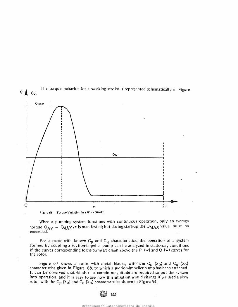
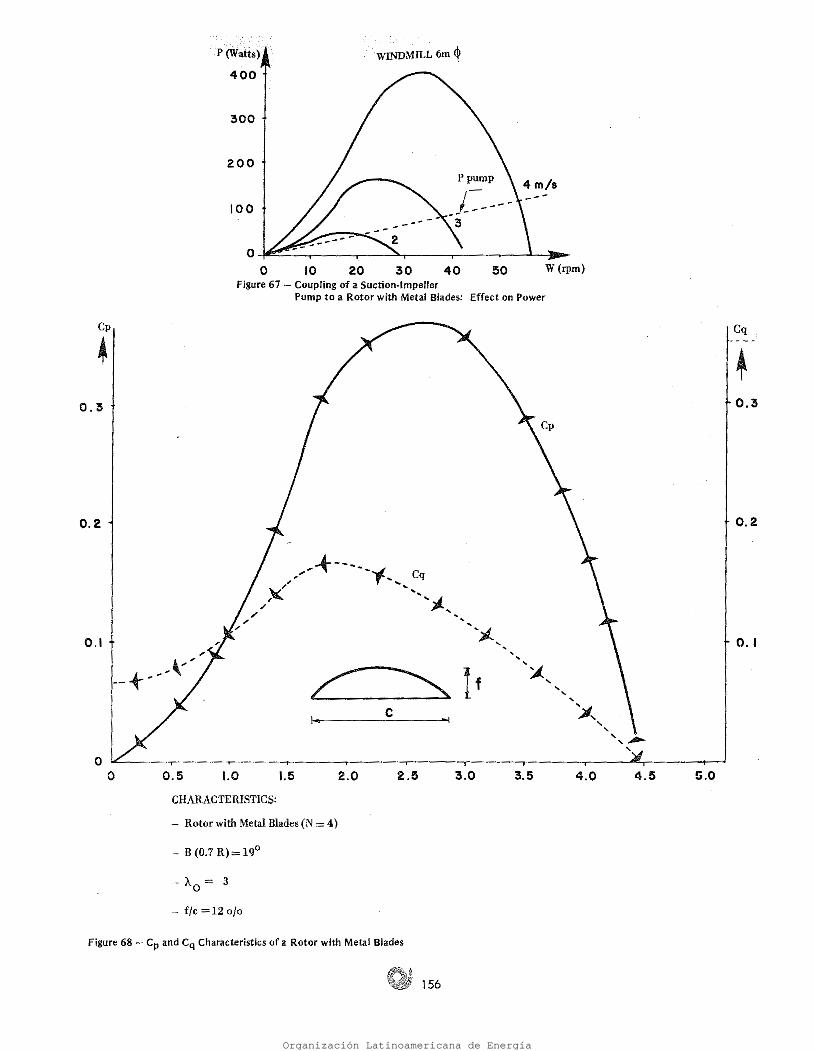
Figure 67 shows a rotor with metal blades, with the Cp {A.0) and Cq (A.o) characteristics given in Figure 68, to which a suctionimpeller pump has been attáched. lt can be observed that winds of a certain magnitude are required to put the system into operation, and it is easy to see how this situation would change if we used a slow rotor with the Cp ('A0) and Cq (A.0) characteristics shown in Figure 64:

For a rotor with known Cp and Cq characteristics, the operation of a system formed by coupling a suctionimpeller pump can be analyzed in stationary conditions if the curves corresponding to the pump are drawn above the p (w) and Q (w) curves for the rotor.

When a pumping system functions with continuous operation, only an average torque QA v = <:MAX /rr is manifested; but during startup the 0MAX value must be exceeded.

tt

Figure 66 Torque Variation in a Work Stroke

o

1 1 r Qw

The torque behavior for a working stroke is represented schematically in Figure 66. Q


4.5 4.0 3.5

156

Figure 68 Cp and Cq Characteristics of a Rotor with Metal Blades

f/c =12 o/o

"o= 3

B (0.7R)=19°

Rotor with Metal Blades (N = 4)

CHARACTERISTICS:

2.0 1.5 1.0 0.5 5.0 3.0 2.5

0.1

0.2

0.3

Cq ,

' ... ... ~

' ' ... ' ~ ...

' ' ',"""""' ' o

o

e

0.1

0.2

0.3

Cp

~

Figure 67 Coupling of a Suctionlmpeller Pump to a Rotor with Metal Blades: Effect on Power

30 20 W (rpm) 50 Q-1"'::::.;:_~-.-~~-T~~~.--~~--r-~~-.-~_._---:~

o 40 10

100

200

300

. . . : ·. ~ . : : .

. WINDMILL 6m ~ ~<Wa~M· 400


157

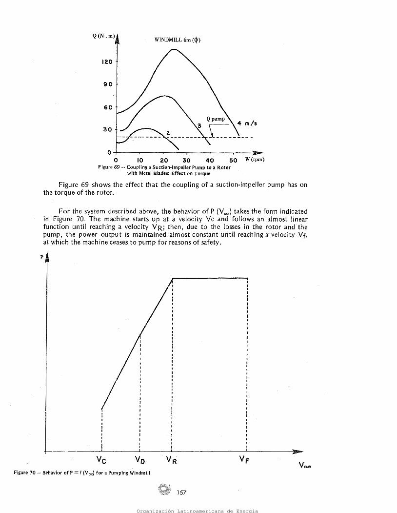
Figure 70 Behavior of P = f (V c.J for a Pumping Windmill

p

F or the system described above, the behavior of P (V 00) takes the form indicated in Figure 70. The machine starts up at a velocity Ve and follows an almost linear function until reaching a velocity VR; then, due to the losses in the rotor and the pump, the power output is maintained almost constant until reaching a· velocity Vf, at which the machine ceases to pump for reasons of safety.

Figure 69 shows the effect that the coupling of a suctionimpeller pump has on the torque of the rotor.

Figure 69 Coupling a SuctionImpeller Pump to a Rotor with Metal Blades: Effect on Torq.ue

50 W(rpm) 40 30 20 10 o

WINDMILL 6m ((j>) Q (N. m)


158

= power (watts) = water density (103 kg/m3)

= pumping height (rn) = acceleration of gravity (9.81 m/s2)

water flow (rn3 /hr)

Where:

{3-7) Pw = Pw. g. H. q

The power required to pump water to a given height is determined as follows:

= power (watts) design velocity at which the rotorpurnp combination works ata celerity with a maximurn Cp (m/s) design celerity (dimensionless) celerity without load (dimensionless) efficiency of transmission and pump (dimensionless) power coefficient at Xod (dimensionless) air density

= ·· rotor diameter (m) = wind velocity (m/s)

Xod A.omax = r¡

Cpmax = p Dr Voo

Where:

(3-6) Pe 1 1 o2 Vrr' = pmax · 11 • 2 · P • 4 · 1T • r · D

· lf we assume a linear function for Cq and A.0, the P (V 00) characteristic of a system takes the following form:

cutout velocity design velocity nominal (rated) velocity cutin velocity

For Figure 70:


• . 159

In both cases, the influence on both the design velocity and the total amount of water pumped can be appreciated.

Taking the expressions for the Weibull distribution, given in bibliographical references B-S and 3-7, we have theoretically calculated the effect of two distributions with the same scale factor C (3.55 m/s) and different average velocities V (3.16 and 3.26 m/s) for a windmill having a diameter of 4 meters (Figure 71.2), as well as the effect of two distributions with the same average velocity V {3.2G m/s) and different scale factors C (Figure 71.6).

3.2 INFLUENCE OF WIND FREQUENCY DISTRIBUTION

With ali the theory expounded up to now, we are in a position to analyze the influence of the various pararneters, both for the wind resource and for the system, in terms of machi ne behavior.

·· ·· for whích ali the terms have already been defined previously. Here, the influence of ·. the different rotor and wind parameters can be observed with respect to .the pumpírg stroke and diameter. · ·

.· (3-9)

·.·. -: .. Ó, : .. ':

4c~max. · .:ow.Vd2 ;* R3 ;?Jp.t ·· ." · X0 .. ·... . Pw&H .· ...

.............. · ·.i=~9n1. this.·l~st e~ptession,•it·cari be (")bs.e.rved.tnaf the w~_te(flow'pu¡)lped· by the .: systeqj'.J~:<infll)ené~(i· qy·. pÚÜJping helght,:aeródynami~ effi((iency, rot9r.ge'omefry. ''·de$ign,·yel.()cjty.ánp .. wü1d··frecjÜerwy·'distributiOQ.· lftbis expression )s.:· mül.tipOed.by .

·•.·• the (Jjstrib,utJon. pf,' the ... wincfve19ciW. 'freqUency.· in-'the place úndér consíderattcn, the .. ·.• •. volume of.water pu_mpeddvrif"\gthe Pirk>dinquesfü:m can.be determined ... · · · ··

. ,' - :··· .. · ... ·' -- - .... -. . -· ..... · . .· ··'.". ·.···. :- '· _"'.', ', ... ,', '_', '.·

".· .... ··.·· In StábJe cpnditi()ns, P ~:·Pw. The~, .ifwe put Eq~atio~s (3-6) and (3-7) .. in equal <formsand .. solve for;<t : · · · · ·· ·· ·. · .· · · · · · · · · ·· ·


1_60

Figure 72 - lnfluence of Pumping Height and Rotor Diameter

2000 q (m3/month) 1500 1000 500 o+-~~~--,~~~~..,.-~~~~....-~~~~--'~~--->J._

o

20

30

40

!50

60

· dR = 5m. dR =°4m. 10

· · Tlie effect of variations in these pararneters has been calcu lated for a régimen -. ofwinds with K = 1.75 and C.= 3.59. The results can be appréciated in Figure 7

H(m.)

(b) (a) . . ., ~igure n ,.:.1'ni1~ef1ce of Wind Frequ~~cy Distributlon .

. 3.3 . INHUENCE OFPUMPINGHEIGHTJ.\NÓ RÓTOROIAMETER .

7.0 .. ·:·• · V d(m/s~

1 1. >61 .. ~·.·····'ºº .. ~· s. .. s.s··e~ci ., " ··\lci (m/s)

j . 1 :u ... · 4.0 ·.· 4.5 ·•

~'O·~ , ·: ·. 5 ..

.2000

600

2500 e= 3.599m/s Dr =·4.0 m 500

V =3.26 m/s Dr =4.0 m

i5oo

3500 roo

3000 )00


161

In Figure 74, the graphs shown in Figure 71 have been superposed on those corresponding to a Crete windmill.

3~5 . INFLUENCE OF ROTOR AERODYNAMICS

Figure 73 lnfluence of Desígn Velocity

D

F

----P(Vdt)

p (V d2)

P,F

In Figure 73, a functiorr P (V°.°) for a given system has been superposed; on the frequency distribution curve for a given place. lt can be observed that with a lower design velocity there are more hours of functioning (and a lesser water flow), as can be gathered from Figure 71. This fact can be important in sorne applications, as for example 'Aflen water is going to be pumped for household use.

3.4 INFLUENCE OF DESIGN VELOCITY


· · · · lt can be observed that on increasing the éonstant r6tor diameter, the stroke Is. . . decreased when the pistan diarneter is increased; .this effect is more prortOuncedV{ith\ .. ··

. srnaller pum p. diameters. · · ·

... <·A ·in~re ~><haustíve studyof thepümpused toralse ~at~rispr~sentedihdhap~~r ·.· .. 5 of this document> ·· .. • · · · :· . ; ·· · ·· · · ·

.: .. ·. Oi16~'.}

. 20 :. 40 .

PISTONDIAMETE~·

.· 3.7 INFLUENCE OF PUMP DIAMETER

O= 4rn ·¡s C= 3.59 mft

< v 1: 3.26 rll/a)

. . . . . -.

·:/C7"· :· ... ···: ··: .. ·· ·.· .. .'. .: -. · . _.. . . . . :

. · .. ·.·.· .· . Metal Crete. . ·· t=: 3000


REVISTA 27 ENEROETICA - Centro de …biblioteca.olade.org/opac-tmpl/Documentos/hm000245.pdf · Si...

Documents

Transcript of REVISTA 27 ENEROETICA - Centro de …biblioteca.olade.org/opac-tmpl/Documentos/hm000245.pdf · Si...