Revisiting the Expectations Hypothesis of the Term Structure of Interest Rates

George Bulkley1, Richard D. F. Harris1 and Vivekanand Nawosah2

Paper Number: 08/02

May 2008

Abstract

The expectations hypothesis of the term structure has been decisively rejected by a large empirical literature that spans several decades. In this paper, using a newly constructed dataset of synthetic zero coupon bond yields, we show that evidence against the expectations hypothesis became very much weaker following the widespread acceptance of its empirical failure to describe the behavior of interest rates in the early 1990s. Indeed, in the period 1991-2004, the expectations hypothesis cannot be rejected for most bond maturities. These results are consistent with the idea that asset pricing anomalies tend to disappear once they are widely recognized. Keywords: Expectations hypothesis of the term structure of interest rates; Forward yields; Yield spreads; Campbell and Shiller tests; Vector autoregression. 1 Xfi Centre for Finance and Investment, University of Exeter. 2 Department of Accounting and Finance, University of Essex. We gratefully acknowledge financial support from the ESRC under research grant ACRR2784. We would also like to thank seminar participants at the University of Exeter, the University of Essex and Queen’s University of Belfast.

2

1. Introduction

The expectations hypothesis of the term structure of interest rates states that the yield on a

long bond is equal to the average expectation of the short yield over the life of the long

bond, plus a constant risk premium. The expectations hypothesis (henceforth EH) has a

number of important implications for the relationships between bond yields and their

co-movement over time, and is one of the most widely tested theories in financial

economics. The implications of the EH for the movement of bond yields have been

investigated using a wide range of tests in a literature that spans several decades. The

earliest tests of the EH examine the predictive ability of forward yields that are implicit in

the term structure, and find that although informative, forward yields are biased predictors

of future interest rates (Fama, 1984; Fama and Bliss, 1987). However, perhaps the most

striking evidence against the EH is provided by Campbell and Shiller (1991), who develop

a range of tests based on the yield spread between bonds of different maturities. Using both

single equation and VAR-based approaches, Campbell and Shiller (1991) find virtually no

evidence in support of the EH. Indeed, in many cases, bond yields appear to move in a

direction that is opposite to that predicted by theory.1 Subsequent studies have shown that

this rejection is not confined to the US.2

A naturally important question is whether the empirical failure of the EH can be accounted

for within the rational expectations paradigm, or whether it constitutes evidence of an asset

pricing anomaly. To this end, there has been a sustained search for a ‘rational’ explanation

for the rejection of the EH. A limitation of standard tests of the EH is that they assume that

the risk premium is constant. In the presence of a time-varying risk premium, tests of the

EH are potentially biased in favor of its rejection. A number of studies have explored this

possibility, and indeed tests that allow for a time-varying risk premium have generally

produced weaker rejections of the EH (see, for example, Fama, 1984; Evans and Lewis,

1994; Mankiw and Miron, 1996). However, the results of these studies are sensitive to the

choice of proxy for the risk premium, the bond maturities considered and the sample period

used.3 On balance, it would appear that while the presence of a time-varying risk premium

1 See also Shiller (1979), Shiller et al. (1983), Campbell and Shiller (1984), Mankiw and Summers (1984), Mankiw (1986) and Campbell (1995). 2 See, for example, Hardouvelis (1994). 3 See also Shiller et al. (1983), Jones and Roley (1983), Backus et al. (1987), Simon (1989),

3

might partially explain the empirical failure of the EH, the scale of the rejection is simply

too large to be fully accounted for in this way (see Backus et al., 1994; Dai and Singleton,

2000; Duffee, 2002).

Another potential explanation for the rejection of the EH is that there are statistical

problems with the tests that are commonly used in the literature. For example, Stambaugh

(1988) shows that measurement error in the long yield potentially biases tests of the EH in

favour of its rejection. However Campbell and Shiller (1991) show that the EH is strongly

rejected even after allowance is made for such measurement error through the use of

instrumental variables. Bekaert et al. (1997) identify a further small sample bias in tests of

the EH, and show using Monte Carlo simulation that even in the relatively large samples

that are typically used in empirical work, this bias remains significant.4 However the

direction of the bias is such that the empirical evidence actually represents unambiguously

stronger evidence against the EH than asymptotic theory would imply.5

In this paper, we contribute to this debate by examining whether the empirical evidence

against the EH has weakened over time. If there exists a rational explanation – yet to be

uncovered – for the empirical rejection of the EH, there is no reason to expect this rejection

to be any less evident in later samples, even following the widespread acceptance of the

evidence against the EH. However, if the reported failure of the EH is simply an asset

pricing anomaly, this would imply the existence of potentially profitable arbitrage

opportunities. With the evidence against the EH firmly in the public domain following the

publication of Campbell and Shiller (1991), we would expect market participants to trade

in such a way as to restore bond yields to the equilibrium values required by the EH, in

which case one would expect the evidence against the EH to have weakened over time.

Tests of the EH are greatly simplified by the use of zero coupon bond data. Since the

availability of zero coupon bonds is limited in practice, researchers must rely on synthetic

data on zero coupon bond yields that are imputed from the yields of coupon-paying bonds.

The majority of studies for the US (including Campbell and Shiller, 1991) employ the Froot (1989), Tzavalis and Wickens (1997) and Harris (2001). 4 This bias is related to the downward bias of the OLS estimator of the autoregressive coefficient in the short yield model (see Kendall, 1954). 5 For further discussion of the statistical properties of tests of the EH, see also Bekaert and Hodrick (2001), Kool and Thornton (2004) and Thornton (2005).

4

monthly synthetic zero coupon bond yield data of McCulloch (1990) covering the period

December 1946 to February 1987, subsequently updated by McCulloch and Kwon (1993)

to February 1991. We extend the zero coupon bond yield data of McCulloch and Kwon

(1993) to December 2004 using data on coupon paying bonds from the CRSP US Treasury

Database. We update the evidence on the EH by applying the yield spread tests of

Campbell and Shiller (1991) and the earlier forward yield tests of Fama (1984) and Fama

amd Bliss (1987) to the extended sample as well as to two sub-samples that comprise the

McCulloch and Kwon (MK) sample, January 1952 to January 1991, and the new sample,

February 1991 to December 2004. Our results are striking: we find that the evidence

against the EH is very much weaker in the 1991-2004 period than in the original MK

sample. Indeed, in many cases, the EH cannot be rejected in the later data. For example,

using the Campbell and Shiller (1991) ‘long yield’ regression, the EH is rejected for all

bond maturities in the MK sample, but for only the shortest bond maturity in the post-MK

sub-sample. Across all of the tests that we use, and for almost all of the bond maturities

that we consider, the estimated coefficients in the EH tests are substantially closer to unity

(their value under the EH) in the post-MK sub-sample than they are in the MK sub-sample.

Our results therefore offer new hope for the EH as a description of the relationships

between the yields of bonds of different maturities and their co-movement through time.

The outline of this paper is as follows. In the following section, we summarize the theory

of the EH and the empirical tests that have been widely used to test it. Section 3 describes

the construction of the new dataset of zero-coupon bond yields that we use in the empirical

analysis. In Section 4, we replicate all of the conventional tests of the EH using the

extended dataset and the two sub-samples. Section 5 concludes.

2. Theoretical Background: The Expectations Hypothesis

Consider an n-period zero coupon bond with unit face value, whose price at time t is tnP , .

The yield to maturity of the bond, tnY , , satisfies the relation

ntn

tn YP

)1(1

,, += (1)

5

or, in natural logarithms,

tntn nyp ,, −= (2)

where )ln( ,, tntn Pp = and )1ln( ,, tntn Yy += . If the bond is sold before maturity then the

log m-period holding period return, mmtnr +, , where nm < , is defined as the change in log

price, tnmtmn pp ,, −+− , which using (2) can be written as

mtmntn

tnmtmnmtn

ymnnyppr

+−

+−+

−−=

−=

,,

,,,

)( (3)

The expectations hypothesis states that the expected holding period return for bonds of

different maturities should be equal, except for a risk premium. Combined with the rational

expectations hypothesis, the expectations hypothesis of the term structure has a number of

important implications for the relationships between bond yields, and their movement over

time. In particular, the expectations hypothesis states that the expected n-period return on

an investment in a series of one-period bonds should be equal to the (certain) n-period

return on an n-period bond, which implies that the n-period long yield should be an average

of the expected short yield over the following n periods, plus a constant risk premium. That

is

n

n

iitttn yE

ny φ+= ∑

−

=+

1

0,1, )(1 (4)

where nφ is the risk premium and (.)tE is the expectation conditional on the time t

information set. The relation given by (4) is known as the expectations hypothesis (EH).

The most well-known tests of the EH are those of Campbell and Shiller (1991). These tests

focus on the predictive ability of the (log) yield spread between long maturity and short

maturity bonds, defined as ttntn yys ,1,, −= . In particular, combining equation (4) for two

adjacent bond maturities and then rearranging, gives

6

nntntnttnt nnyy

nyyE φφ

1)(

11

111,1 −−+−

−=− −+− (5)

which states that the yield spread should predict the following period’s expected change in

the yield on the long bond. Alternatively, rearranging equation (4) gives

nttnt

n

i

itt yyn

nyn

yEφ+−

−=−

−∑−

=

+ )(11 ,1,,1

1

1

,1 (6)

which states that the yield spread should predict the cumulative expected change in the

short yield over the life of the long bond. These two predictions of the EH can be tested

with regressions of the form

1,11,11,1,1 )(1

1++− +−

−+=− tttntntn yy

nyy εβα (7)

1,21,22,1

1

1

,1 )(11 +

−

=

+ +−−

+=−−∑ tttnt

n

i

it yyn

nyny

εβα (8)

If the EH holds then the coefficients 1β and 2β should be equal to unity, while the

intercepts 1α and 2α capture the constant risk premium terms. Estimating regression (7)

generates a very significant rejection of the EH. The coefficient 1β is typically found to

be significantly less than unity, and falls with the maturity of the long bond. For long

maturity bonds, it is significantly less than zero. The coefficient 2β in equation (8), in

contrast, is typically found to be significantly less than unity for short maturity bonds, but

it rises with maturity. For long maturity bonds, it is often found to be significantly greater

than unity. (see, for example, Campbell and Shiller, 1991; Bekaert et al., 1997; Bekaert and

Hodrick, 2001).6 The fact that regression (7) delivers a significant rejection of the EH but

regression (8) does not, at least for some bond maturities, is ostensibly puzzling (see, for

6 Campbell and Shiller (1991) also test the EH using analogous regressions based on the yield spread between all possible pairs of bond maturities, tmtntn yys ,,, −= , for n between two months and 120 months and for m between one month and 60 months. The EH is strongly rejected for almost all pairs of bonds.

7

example, Campbell, 1996). However, Bekaert et al. (1998) show that while both regression

(7) and regression (8) are subject to small sample biases, the bias is much greater for

regression (8) than it is for regression (7). Once this small sample bias is allowed for,

regression (8) also delivers a decisive rejection of the EH.

Campbell and Shiller (1991) also propose a vector autoregression (VAR) approach, based

on Campbell and Shiller (1987). In particular, a pth-order VAR for the n-period spread,

tns , , and the change in the short yield, ty ,1∆ , can be written in companion form as

ttntn AZZ ,41,, ε+= − (9)

where tnZ , is a (2p x 1) vector comprising the current value and p – 1 lags of tns , and the

current value and p – 1 lags of ty ,1∆ , A is a (2p x 2p) matrix of parameters and t,4ε is a

(2p x 1) vector of errors. Forecasts of the n-period spread and the change in the short yield

are then given by tni

itn ZAZ ,,ˆ =+ . Using the EH relation (4), we can then define the

‘theoretical’ spread as

tnn

tn ZAAIAInIAes ,11

, )1]())()(/1(['~ −− −−−−= (10)

where e is a (1 x 2p) ‘selection’ vector, such that tntn sZe ,,' = and I is the (2p x 2p)

identity matrix. Since the conditioning information in the VAR includes the current

n-period spread, which itself embodies the market’s expectations of future short yields over

the life of the long bond, the theoretical spread should be equal to the actual spread.

Campbell and Shiller (1991) suggest the following two tests of the EH. Firstly, the

correlation between the theoretical spread and the actual spread should be equal to unity.

Secondly, the ratio of the standard deviation of the theoretical spread to the standard

deviation of the actual spread should be equal to unity. Using the McCulloch (1987) dataset,

Campbell and Shiller (1991) find that while the correlation coefficient is indeed close to

unity, the standard deviation ratio is typically around 0.5, thus strongly rejecting the EH.

A final way to test the EH focuses on the predictive ability of the expectations of future

spot yields that are implicit in the term structure of interest rates. By combining expression

8

(4) for bonds of two different maturities, we can define the m-period forward yield for an

n-period bond as

nmmnyEnmyymnf

mtmnmtnt

tmtmnmtn

/))(()(/))((

,,

,,,

φφ −++=

−+=

++

+ (11)

Earlier tests of the EH directly examined whether the forward rates that are implied by the

term structure are unbiased predictors of future interest rates. This can be tested using a

regression of the form

mttnmtntnmtn yfyy ++ +−+=− ,3,,33,, )( εβα (12)

If forward rates are unbiased then the slope coefficient, 3β , should be equal to unity, while

the constant risk premium differential is captured by the intercept, 3α . This regression has

been estimated for values of m of between one month and twenty years, and for values of n

of between one month and five years. While forward yields clearly contain information that

is relevant for future spot yields, the estimated coefficient, 3β , is usually found to be

significantly less than unity (see, for example, Fama, 1984; Fama and Bliss, 1987; Fama

2006).

3. Zero Coupon Bond Yield Data

In this paper we use monthly zero-coupon bond yields on US Treasury securities for the

period January 1952 to December 2004.7 Many of the empirical studies of the EH

described in the preceding section make use of the McCulloch (1990) monthly US term

structure data set, or the subsequently extended data set of McCulloch and Kwon (1993).8

The McCulloch and Kwon (1993) data comprise monthly time series of estimated

zero-coupon yields, par bond yields and instantaneous forward rates (and their respective

7 Although data are available from December 1946, the quality of the estimated data improves significantly after the Treasury Accord of 1951 and so only data after this period are used, as recommended by McCulloch and Kwon (1993). 8The McCulloch and Kwon (1993) zero-coupon bond yield dataset can be found at www.econ.ohio-state.edu/jhm/ts/mcckwon/mccull.htm.

9

standard errors) from December 1946 to February 1991. The data are continuously

compounded and recorded as annual percentages. Synthetic zero-coupon bond yields are

available for 56 maturities from overnight to 40 years.

For the purpose of this paper, we have updated the McCulloch and Kwon (hereafter MK)

dataset to December 2004. The data are constructed using the tax-adjusted cubic spline

method of McCulloch (1975).9 The raw data were obtained from the CRSP US Treasury

Database and include all available quotations on US Treasury bills, notes and bonds. Data

on tax rates were obtained from the Internal Revenue Service, US Department of

Treasury.10 Since the raw data that we use originate from a different source, it is important

to check the integrity of the resulting estimated zero-coupon bond yields. We therefore

computed zero-coupon bond yields over a six-year overlapping period, August 1985 to

February 1991, and compared these with the corresponding yields reported in the MK data

set.11 Panel A of Table 1 reports summary statistics for the two data sets for the ten bond

maturities that we use in this paper. For all ten bond maturities, the correlation between the

two data sets is in excess of 0.99, and for all except the one month maturity, the correlation

is in excess of 0.999.

[Table 1]

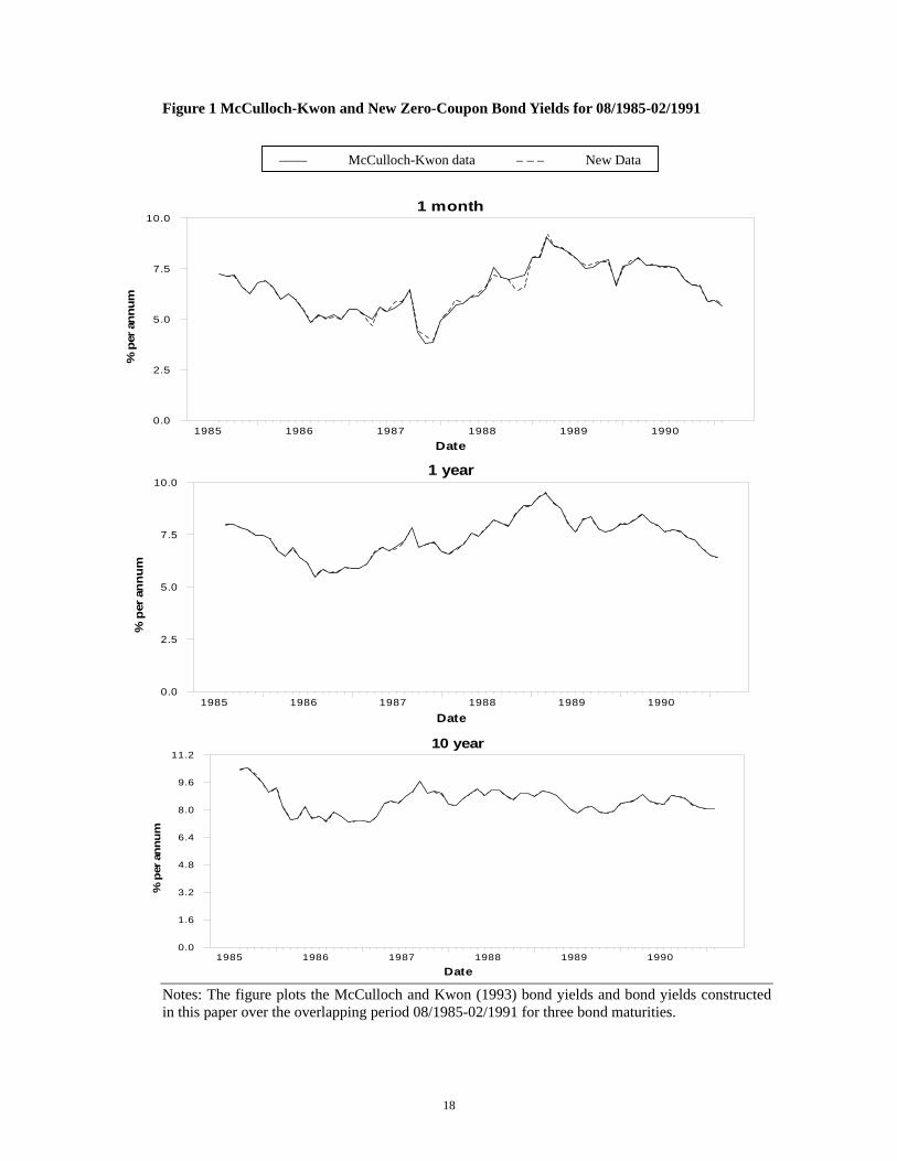
Figure 1 plots the estimated yields for a selection of maturities over the overlapping period.

For maturities greater than one month, there is no discernable difference between the two

data sets. For the one-month maturity, there are some very minor discrepancies that arise

mainly from small differences in the sample of bonds used in the estimation procedure.

Panel B of Table 1 reports summary statistics for the period covered by the MK data

9 The authors are indebted to J. Huston McCulloch for kindly providing the FORTRAN program that fits the term structure of interest rates using the tax-adjusted cubic spline method and for his valuable help in resolving a number of problems associated with the construction of the data set. 10 (www.irs.gov). 11 We choose the start date of August 1985 for the overlapping period on the grounds of convenience. Before this date, there are many more irregular bonds in the raw data which have to be manually deleted. Also, McCulloch and Kwon stopped using long-term callable bonds as from this date. For these reasons, it is easier to match the numbers in the original McCulloch and Kwon data set for August 1985-February 1991.

10

(January 1952 to February 1991), for the post-MK data (March 1991 to December 2004),

and for the combined sample.

[Figure 1]

4. Results

In this section, we report the results of the regression and VAR tests of the EH, applied to (i)

the full sample, January 1952 to December 2004, (ii) the MK sub-sample, February 1952

to January 1991, and (iii) the post-MK sub-sample, February 1991 to December 2004. The

single equation regressions for the forward yield, short yield and long yield, and the two

equations of the VAR for the short yield and the yield spread, are estimated by OLS. For all

of the regressions, we estimate heteroscedasticity adjusted standard errors of the parameter

estimates and, for the regressions with an overlapping dependent variable, we further allow

for serial correlation of a lag order equal to the number of overlapping observations.

Yield Spread Tests

Table 2 reports the estimated parameters from the long yield regression (10) for the full

sample (Panel A) and the MK and post-MK sub-samples (Panels B and C, respectively).

Standard errors are reported in parentheses. The regressions are estimated for long bonds of

maturity n = 3, 6, 9, 12, 24, 36, 48, 60 and 120 months. In Panels A and B of Table 2 we

see that for both the full sample and the post-MK sub-sample, the estimated slope

coefficient is negative and significantly lower than unity for all bond maturities, and the

point estimate falls monotonically with maturity. For all but the three-month bond, the

estimated slope coefficient is not only significantly less than unity, but also significantly

less than zero, implying that long bond yields move in a direction opposite to that implied

by the EH. The results for the MK sub-sample are similar to those reported by Campbell

and Shiller (1991) and Bekaert et al. (1997).

In Panel C of Table 2 we report results for the post-MK sub-sample. In sharp contrast with

the MK sub-sample, the EH is only rejected for the three-month maturity. The estimated

slope coefficient falls with bond maturity, becoming negative at the 48 month maturity, but

not significantly so. For all maturities, the point estimate of the coefficient on the yield

11

spread is closer to unity than the corresponding slope coefficient in the MK sub-sample,

reported in panel B.

[Table 2]

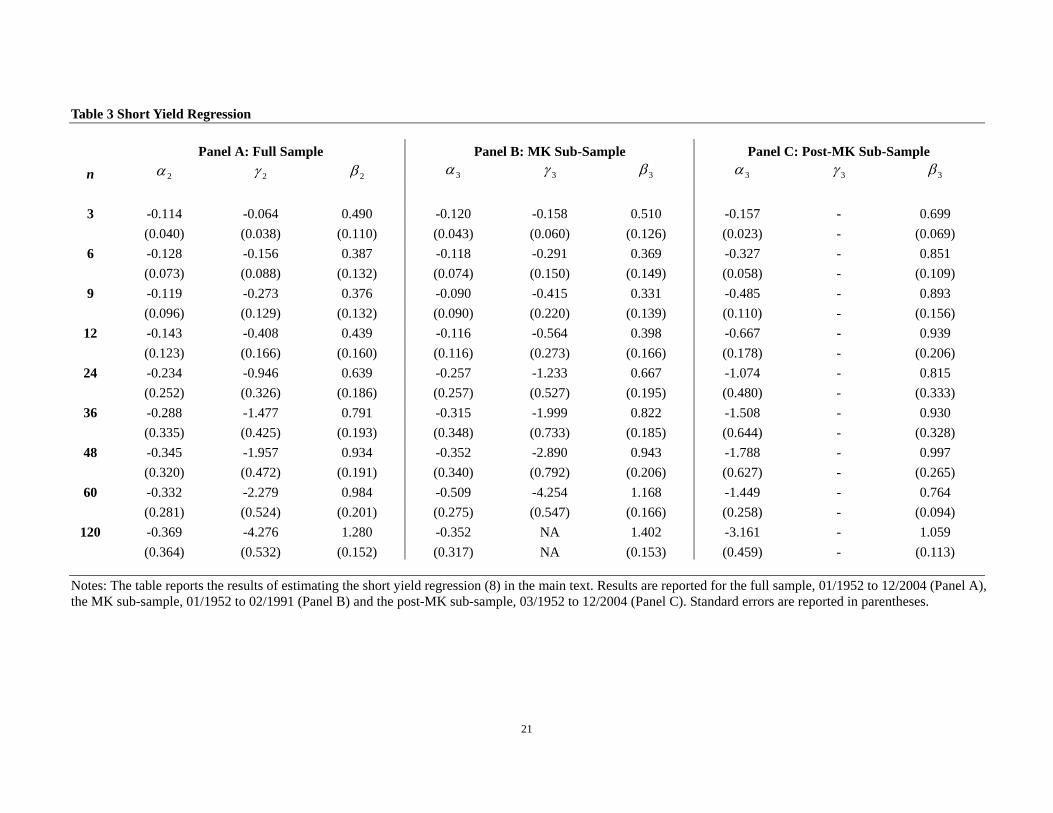
Table 3 reports the estimated parameters from the short yield regression (9). Standard

errors (reported in parentheses) are estimated using the Newey and West (1987) estimator

to allow for the fact that the dependent variable is overlapping. The regressions are

estimated for long bonds of maturity n = 3, 6, 9, 12, 24, 36, 48, 60 and 120 months. For

both the full sample and the MK sub-sample, the estimated slope coefficient is significantly

lower than unity for short maturity bonds, and initially falls with maturity up to nine

months, but then rises with maturity. For the 120-month bond, the coefficient is

significantly greater than unity in the full sample. These results, which are consistent with

those reported by Campbell and Shiller (1991) and Bekaert et al. (1997), represent a strong

rejection of the EH. In the post-MK sub-sample, however, the EH is only rejected for the

three-month maturity and, marginally, the 60-month maturity. For all maturities, except

60-months, the point estimate of the slope coefficient is closer to unity in the post-MK

sub-sample than in the MK sub-sample.

[Table 3]

VAR Tests

Table 4 reports the correlation coefficient and standard deviation ratio for bond maturities n

= 3, 6, 12, 24, 36, 48, 60 and 120 months for the full sample and the two sub-samples. The

VAR was specified with a lag length of four, chosen on the basis of the Schwartz Bayesian

criterion. For the MK sub-sample, the correlation coefficient (measuring the correlation

between observed and theoretical spreads) is significantly lower than unity for maturities

up to 36 months, although at longer maturities the EH cannot be rejected. These results are

consistent with the findings of Campbell and Shiller (1991). A similar result holds in the

full sample. However for the post-MK sub-sample the correlation coefficient is not

significantly different from unity for any bond maturity. The test of the EH based on the

standard deviation ratio between the observed and theoretical spread decisively rejects the

EH in the full sample and the MK sub-sample. In particular, it is significantly different

12

from unity in all cases, again consistent with the findings of Campbell and Shiller (1991).

In the post-MK sub-sample, the EH is still often rejected, but it is clear that the rejection is

very much weaker. In all cases, the estimated standard deviation ratio is closer to unity in

the post-MK sub-sample than it is in the MK sub-sample, and for two maturities – nine

months and 12 months – it is not significantly different from unity.

[Table 4]

Forward Yield Tests

Table 5 reports the estimated parameters from the forward yield regression (6) for the

one-month bond maturity (n = 1 month) and forward horizons of between one month and

one year (m = 1, 3, 6, 9 and 12 months), for the full sample (Panel A) and the two

sub-samples (Panels B and C). Standard errors are reported in parentheses. In the full

sample, and in the MK sub-sample, the estimated slope coefficient is significantly less than

unity for all horizons, at first declining with maturity and then rising with maturity.

Consistent with the results of Fama (1984), the EH is very strongly rejected. However, for

the post-MK sub-sample, while the EH clearly still does not hold in all cases, its rejection

is very much weaker. In particular, we cannot reject the null hypothesis that the slope

coefficient is equal to one except for the one-month horizon, and only marginally for the

three-month horizon. In all cases, the estimated slope coefficient is again closer to unity in

the post-MK sub-sample than it is in the MK sub-sample.

[Table 5]

Table 6 reports the results of the same regression for the one-year bond maturity (n = 12

month) and a forward horizons of between one and ten years (m = 12, 24, 36, 48, 60 and

120 months). For both the full sample, and the MK sub-sample, the estimated slope

coefficient is significantly less than unity for the 12-month and 24-month horizons, but

significantly greater than unity for longer horizons up to 60 months. For the 120-month

horizon, the coefficient is insignificantly greater than unity for the full sample, while for

the MK sub-sample, it is insignificantly less than unity. The results for the MK sub-sample

are very similar to those reported by Fama and Bliss (1987) (which covers the period June

1953 to December 1985), and strongly reject the EH. For the post-MK sub-sample, the

13

estimated slope coefficient is closer to unity for the 12-month and 24-month forward

horizons and for the latter, the EH cannot be rejected. However, for three of the four

remaining horizons (36, 48 and 60 months), the estimated slope coefficient is significantly

greater than unity, in contrast with the MK sub-sample, where it is lower than unity for

these horizons. For the 120-month horizon, the estimated slope coefficient is significantly

less than unity. Thus, the EH is still rejected for most forward horizons, but the nature of

the rejection has changed substantially between the MK and post-MK sub-samples. The

results for the one-year forward yield tests reported here for the full sample and the

post-MK sample are consistent with Fama (2006), who extends the analysis of Fama and

Bliss (1987) to include the additional period January 1986 to December 2004, and

considers forward horizons of 12, 24, 36 and 48 months. For the full sample, the estimated

coefficients are almost identical to those reported by Fama for the period June 1953 to

December 2004, while for the post-MK sub-sample, the estimated coefficients reported

here are similar to those reported by Fama for the period January 1986 to December 2004.

[Table 6]

5. Conclusion

By 1991 there was overwhelming evidence that the EH did not describe how long yields

are determined in practice. Indeed this verdict on the EH was so widely accepted that there

has been little new evidence on the EH since the landmark paper of Campbell and Shiller

(1991). The purpose of this paper is to fill this gap in the literature. Using data on coupon

paying bonds from the CRSP US Treasury Database, we extend the zero coupon bond yield

data of McCulloch and Kwon (1993), which ended in February 1991, to December 2004.

We apply a range of tests to short yields, long yields and forward yields using both the

extended sample, and sub-samples that comprise the McCulloch and Kwon (1993) data,

and data for the more recent period, 1991-2004.

We find that the evidence against the EH is very much weaker in the 1991-2004 period

than in the original McCulloch and Kwon sample. Indeed, in the majority of cases, the EH

can no longer be rejected in the later sample. For example, the EH predictions for changes

in the long yield are rejected for every bond maturity in the McCulloch and Kwon sample

but only rejected for the shortest maturity bond in the 1991-2004 period. A plausible

14

explanation for this finding is the publication of Campbell and Shiller’s (1991) milestone

paper on the EH, which perhaps marked the point at which the unambiguous rejection of

the EH became widely accepted by the finance community. In attempting to exploit the

arbitrage opportunities that the rejection of the EH reported by Campbell and Shiller (1991)

implies, it could be argued that market participants helped to restore bond yields to the

equilibrium values required by the EH. These results are consistent therefore with the

original evidence against the EH being interpreted as an anomaly, since if the earlier

rejections were a consequence of some rational mechanism, as yet unidentified, then there

is no reason for this mechanism not to affect the empirical results in exactly the same way

in the later time period.

These results also provide further support for the idea that anomalies are transitory, and

that they tend to be eroded once they become public information. For example, the ‘size’

effect in equity returns was well-documented by a number of important papers published in

the early 1980s (for example Banz, 1981). However, following the publication of these

papers – and the emergence of this anomaly into the public domain – the size effect was

greatly diminished (see, for example, Schwert, 2003). A plausible explanation for the

disappearance of the size effect is that once the arbitrage opportunities that it implied

became widely known, market participants who exploited these arbitrage opportunities

restored equity prices to their fair values in respect of firm size. In the present context,

rejection of the EH implies the existence of profitable arbitrage opportunities. Once these

became widely known, as they did following the publication of Campbell and Shiller’s

milestone paper, one would expect market participants to exploit these opportunities and

thus restore bond yields to levels that are implied by the EH. Whether or not this explains

the findings reported here, our results offer new hope for the EH as a description of the

relationships between the yields of bonds of different maturities and their co-movement

through time.

15

References

Backus, D.K., A.Gregory, and S.E.Zin, 1994, “Risk Premiums in the Term Structure: Evidence from Artificial Economies" Journal of Monetary Economics 24 371-399. Bekaert, G., and R. Hodrick, 2001, “Expectations Hypothesis Tests”, Journal of Finance 56, 1357-1394. Bekaert, G., R. Hodrick and D. Marshall, 1997, “On Biases in Tests of the Expectations Hypothesis of the Term Structure of Interest Rates,” Journal of Financial Economics 44, 309-348. Campbell, J., 1995, “Some Lessons from the Yield Curve,” Journal of Economic Perspectives 9, 125-152. Campbell, J., and R. Shiller, 1984, “A Simple Account of the Behavior of Long Term Interest Rates,” American Economic Review, Papers and Proceedings 74, 44-48. Campbell, J., and R. Shiller, 1987, “Cointegration and Tests of Present Value Models,” Journal of Political Economy 95, 1062-1088. Campbell, J., and R. Shiller, 1991, “Yield Spreads and Interest Rate Movements: A Bird's Eye View,” Review of Economic Studies 58, 495-514. Dai Q. and K. Singleton, 2000, "Specification Analysis of Affine Term Structure Models", Journal of Finance, 50, 1943-1978. DeBondt, W. F. M., and R. H. Thaler, 1985, “Does the Stock Market Overreact,” Journal of Finance 40, 557-581. DeBondt, W. F. M., and R. H. Thaler, 1987, “Further Evidence on Investor Overreaction and Stock Market Seasonality,” Journal of Finance 42, 3, 557-581 Duffee, G., 2002, “Term Premia and Interest Rate Forecasts in Affine Models” The Journal of Finance, 57, 405-443. Evans, M., and K. Lewis, 1994, “Do Stationary Risk Premia Explain It All? Evidence from the Term Structure” Journal of Monetary Economics 33, 285-318. Fama, E., 1984, “The Information in the Term Structure” Journal of Financial Economics 13, 509-528. Fama, E. F., 1998, “Market Efficiency, Long Term Returns, and Behavioral Finance,” Journal of Financial Economics 49, 283-306. Fama, E. F., 2006, “The Behavior of Interest Rates,” Review of Financial Studies 19, 359-379. Fama, E. F. and R. R. Bliss, 1987, "The Information in Long-Maturity Forward Rates," American Economic Review 77, 4, 680-692.

16

Froot, K., 1989, “New Hope for the Expectations Hypothesis of the Term Structure of Interest Rates,” Journal of Finance 44, 283-305. Hardouvelis, G., 1994, “The Term Structure Spread and Future Changes in Long and Short Rates in the G7 Countries: Is There a Puzzle?” Journal of Monetary Economics 33, 255-283. Harris, R. D. F., 2001, “The Expectations Hypothesis of the Term Structure and Time Varying Risk Premia: A Panel Data Approach”, Oxford Bulletin of Economics and Statistics 63, 233-245. Jones, D., and V. Roley, 1983, “Rational Expectations and the Expectations Model of the Term Structure: A Test Using Weekly Data,” Journal of Monetary Economics 12, 453-465. Kool, C., and D. Thornton, 2004, “A Note on the Expectations Theory and the Founding of the FED”, Journal of Banking and Finance 28, 3055-68 Mankiw, N., 1986, “The Term Structure of Interest Rates Revisited,” Brookings Papers on Economic Activity 1, 61-96. Mankiw, N., and J. Miron, 1986, “The Changing Behavior of the Term Structure of Interest Rates,” Quarterly Journal of Economics 101, 211-228. Mankiw, N., and L. Summers, 1984, “Do Long Term Interest Rates Overreact to Short Term Interest Rates?” Brookings Papers on Economic Activity 1, 223-242. McCulloch, H., 1990, “U. S. Government Term Structure Data,” in Friedman, B., and Hahn, F. (eds.), The Handbook of Monetary Economics (Amsterdam: North Holland). McCulloch, H., and H. Kwon, 1993, “U. S. Term Structure Data, 1947-1991,” Working Paper 93-6, Ohio State University. Newey W. K. and K. D. West, 1987, “A Simple, Positive Definite, Heteroskedasticity and Autocorrelation Consistent Covariance Matrix.” Econometrica 55, 3, 703-708. Schwert, G.W., 2003, “Anomalies and Market Efficiency,” in G.M. Constantinides, M. Harris, and R.M. Stulz, (eds.), Handbook of the Economics of Finance, North Holland, Amsterdam. Shiller, R., 1979, “The Volatility of Long Term Interest Rates and Expectations Models of the Term Structure,” Journal of Political Economy 82, 1190-1219. Shiller, R., J. Campbell and K. Schoenholtz, 1983, “Forward Rates and Future Policy: Interpreting the Term Structure of Interest Rates,” Brookings Papers on Economic Activity 1, 173-217. Simon, D., 1989, “Expectations and Risk in the Treasury Bill Market: An Instrumental Variables Approach,” Journal of Financial and Quantitative Analysis 24, 357-368.

17

Stambaugh, R., 1988, “The Information in Forward Rates: Implications for Models of the Term Structure,” Journal of Financial Economics 21, 41-70. Thornton, D., 2005, “Tests of the Expectations Hypothesis: Resolving the Campbell-Shiller Paradox,” Journal of Money, Credit and Banking, forthcoming. Tzavalis, E., and M. Wickens, 1997, “Explaining the Failure of the Term Spread Models of the Rational Expectations Hypothesis of the Term Structure,” Journal of Money, Credit and Banking 29, 364-380.

18

1 year

Date

% p

er a

nnum

1985 1986 1987 1988 1989 19900.0

2.5

5.0

7.5

10.0

1 month

Date

% p

er a

nnum

1985 1986 1987 1988 1989 19900.0

2.5

5.0

7.5

10.0

10 year

Date

% p

er a

nnum

1985 1986 1987 1988 1989 19900.0

1.6

3.2

4.8

6.4

8.0

9.6

11.2

Figure 1 McCulloch-Kwon and New Zero-Coupon Bond Yields for 08/1985-02/1991

Notes: The figure plots the McCulloch and Kwon (1993) bond yields and bond yields constructed in this paper over the overlapping period 08/1985-02/1991 for three bond maturities.

—— McCulloch-Kwon data – – – New Data

19

Table 1 Summary Statistics

Panel A

n McCulloch-Kwon data (Aug. 1985 - Feb. 1991) New data (Aug. 1985 - Feb. 1991) (months) Mean Std Error Minimum Maximum Mean Std Error Minimum Maximum

Correlation

1 6.528 1.193 3.800 9.043 6.527 1.176 3.948 9.248 0.99125 3 6.936 1.057 5.242 9.053 6.935 1.058 5.243 9.056 0.99963 6 7.104 0.977 5.262 9.279 7.102 0.976 5.261 9.314 0.99975 12 7.388 0.927 5.485 9.490 7.390 0.931 5.488 9.545 0.99953 24 7.726 0.821 5.988 9.454 7.734 0.824 6.003 9.527 0.99938 36 7.918 0.775 6.247 9.417 7.915 0.780 6.218 9.470 0.99923 48 8.046 0.748 6.505 9.559 8.044 0.747 6.535 9.572 0.99967 60 8.149 0.743 6.648 9.859 8.155 0.738 6.775 9.899 0.99930

120 8.486 0.715 7.274 10.459 8.479 0.716 7.271 10.459 0.99957

Panel B

n McCulloch-Kwon data (Jan. 1952 - Feb. 1991) New data (Mar. 1991 - Dec. 2004) Extended data (Jan. 1952 - Dec. 2004) (months) Mean Std Error Minimum Maximum Mean Std Error Minimum Maximum Mean Std Error Minimum Maximum

1 5.314 3.064 0.249 16.210 3.716 1.584 0.773 6.210 4.896 2.842 0.249 16.210 3 5.640 3.143 0.615 15.999 3.908 1.650 0.865 6.291 5.188 2.929 0.615 15.999 6 5.884 3.178 0.685 16.511 4.033 1.668 0.955 6.456 5.401 2.974 0.685 16.511 12 6.079 3.168 0.847 16.345 4.275 1.686 1.034 7.142 5.608 2.963 0.847 16.345 24 6.272 3.124 1.149 16.145 4.672 1.610 1.271 7.569 5.854 2.894 1.149 16.145 36 6.386 3.087 1.412 15.825 4.968 1.487 1.616 7.684 6.016 2.829 1.412 15.825 48 6.467 3.069 1.595 15.847 5.221 1.396 2.017 7.712 6.142 2.786 1.595 15.847 60 6.531 3.056 1.770 15.696 5.387 1.323 2.359 7.911 6.232 2.758 1.770 15.696

120 6.683 3.013 2.341 15.065 5.957 1.118 3.608 8.325 6.493 2.670 2.341 15.065 Notes: The table reports summary statistics for the McCulloch and Kwon (1993) and new zero-coupon bond yield datasets for the ten bond maturities that are used in the paper. Panel A reports summary statistics for the overlapping period 08/1985-02/1991. Panel B reports summary statistics for the two sub-samples 01/1952-02/1991 and 03/1991-12/2004, and for the full sample.

20

Table 2 Long Yield Regression

Panel A: Full Sample Panel B: MK Sub-Sample Panel C: Post-MK Sub-Sample n 2α 2γ 2β 3α 3γ 3β 3α 3γ 3β

3 -0.074 -0.056 -0.098 -0.078 -0.127 -0.068 -0.117 - 0.254 (0.034) (0.041) (0.141) (0.041) (0.065) (0.183) (0.021) - (0.145) 6 0.022 -0.051 -0.565 0.045 -0.046 -0.790 -0.101 - 0.647 (0.036) (0.040) (0.234) (0.044) (0.063) (0.307) (0.021) - (0.230) 9 0.065 -0.083 -0.783 0.091 -0.070 -1.117 -0.101 - 0.773 (0.036) (0.040) (0.318) (0.044) (0.064) (0.417) (0.026) - (0.356)

12 0.068 -0.090 -0.875 0.091 -0.075 -1.244 -0.107 - 0.824 (0.035) (0.039) (0.381) (0.042) (0.063) (0.497) (0.031) - (0.474)

24 0.059 -0.046 -0.886 0.072 -0.033 -1.279 -0.053 - 0.713 (0.030) (0.037) (0.563) (0.035) (0.058) (0.714) (0.043) - (0.880)

36 0.061 -0.040 -1.307 0.070 -0.032 -1.664 -0.028 - 0.094 (0.027) (0.035) (0.691) (0.031) (0.053) (0.852) (0.049) - (1.187)

48 0.060 -0.036 -1.602 0.068 -0.032 -1.988 -0.017 - -0.256 (0.026) (0.034) (0.796) (0.029) (0.049) (0.973) (0.050) - (1.369)

60 0.059 -0.035 -1.823 0.066 -0.033 -2.281 -0.015 - -0.360 (0.024) (0.032) (0.877) (0.027) (0.046) (1.070) (0.049) - (1.511)

120 0.054 -0.033 -2.713 0.062 -0.035 -3.600 -0.011 - -0.615 (0.019) (0.027) (1.227) (0.021) (0.037) (1.518) (0.043) - (2.018)

Notes: The table reports the results of estimating the long yield regression (7) in the main text. Results are reported for the full sample, 01/1952 to 12/2004 (Panel A), the MK sub-sample, 01/1952 to 02/1991 (Panel B) and the post-MK sub-sample, 03/1952 to 12/2004 (Panel C). Standard errors are reported in parentheses.

21

Table 3 Short Yield Regression

Panel A: Full Sample Panel B: MK Sub-Sample Panel C: Post-MK Sub-Sample

n 2α 2γ 2β 3α 3γ 3β 3α 3γ 3β

3 -0.114 -0.064 0.490 -0.120 -0.158 0.510 -0.157 - 0.699 (0.040) (0.038) (0.110) (0.043) (0.060) (0.126) (0.023) - (0.069) 6 -0.128 -0.156 0.387 -0.118 -0.291 0.369 -0.327 - 0.851 (0.073) (0.088) (0.132) (0.074) (0.150) (0.149) (0.058) - (0.109) 9 -0.119 -0.273 0.376 -0.090 -0.415 0.331 -0.485 - 0.893 (0.096) (0.129) (0.132) (0.090) (0.220) (0.139) (0.110) - (0.156)

12 -0.143 -0.408 0.439 -0.116 -0.564 0.398 -0.667 - 0.939 (0.123) (0.166) (0.160) (0.116) (0.273) (0.166) (0.178) - (0.206)

24 -0.234 -0.946 0.639 -0.257 -1.233 0.667 -1.074 - 0.815 (0.252) (0.326) (0.186) (0.257) (0.527) (0.195) (0.480) - (0.333)

36 -0.288 -1.477 0.791 -0.315 -1.999 0.822 -1.508 - 0.930 (0.335) (0.425) (0.193) (0.348) (0.733) (0.185) (0.644) - (0.328)

48 -0.345 -1.957 0.934 -0.352 -2.890 0.943 -1.788 - 0.997 (0.320) (0.472) (0.191) (0.340) (0.792) (0.206) (0.627) - (0.265)

60 -0.332 -2.279 0.984 -0.509 -4.254 1.168 -1.449 - 0.764 (0.281) (0.524) (0.201) (0.275) (0.547) (0.166) (0.258) - (0.094)

120 -0.369 -4.276 1.280 -0.352 NA 1.402 -3.161 - 1.059 (0.364) (0.532) (0.152) (0.317) NA (0.153) (0.459) - (0.113)

Notes: The table reports the results of estimating the short yield regression (8) in the main text. Results are reported for the full sample, 01/1952 to 12/2004 (Panel A), the MK sub-sample, 01/1952 to 02/1991 (Panel B) and the post-MK sub-sample, 03/1952 to 12/2004 (Panel C). Standard errors are reported in parentheses.

22

Table 4 VAR Correlation Coefficient and Standard Deviation Ratio

Panel A: Full Sample Panel B: MK Sub-Sample Panel C: Post-MK Sub-Sample n Correlation SD ratio Correlation SD ratio Correlation SD ratio 3 0.872 0.564 0.857 0.599 0.982 0.709 (0.103) (0.099) (0.138) (0.116) (0.018) (0.083) 6 0.799 0.493 0.728 0.521 0.979 0.875 (0.175) (0.103) (0.277) (0.116) (0.018) (0.124) 9 0.820 0.454 0.724 0.469 0.978 0.930 (0.174) (0.102) (0.310) (0.108) (0.019) (0.168)

12 0.867 0.462 0.797 0.472 0.977 0.940 (0.154) (0.114) (0.313) (0.115) (0.022) (0.205)

24 0.945 0.499 0.917 0.507 0.974 0.764 (0.147) (0.175) (0.362) (0.177) (0.036) (0.220)

36 0.973 0.543 0.962 0.564 0.977 0.637 (0.105) (0.214) (0.214) (0.242) (0.039) (0.218)

48 0.983 0.576 0.975 0.606 0.981 0.571 (0.078) (0.230) (0.132) (0.268) (0.036) (0.221)

60 0.988 0.600 0.983 0.635 0.984 0.545 (0.058) (0.236) (0.086) (0.274) (0.032) (0.228)

120 0.996 0.708 0.994 0.742 0.995 0.559 (0.017) (0.235) (0.020) (0.252) (0.010) (0.249)

Notes: The table reports the correlation coefficient and standard deviation ratio between the actual yield spread and the theoretical yield spread given by equation (10) in the main text. Results are reported for the full sample, 01/1952 to 12/2004 (Panel A), the MK sub-sample, 01/1952 to 02/1991 (Panel B) and the post-MK sub-sample, 03/1952 to 12/2004 (Panel C). Standard errors are reported in parentheses.

23

Table 5 Forward Yield Regression (Forecasts of 1-Month Spot Rates)

Panel A: Full Sample Panel B: MK Sub-Sample Panel C: Post-MK Sub-Sample

m 1α 1γ 1β 1α 1γ 1β 1α 1γ 1β

1 -0.155 -0.054 0.504 -0.164 -0.152 0.528 -0.161 - 0.561 (0.034) (0.043) (0.053) (0.040) (0.067) (0.067) (0.025) - (0.062) 3 -0.198 -0.163 0.434 -0.202 -0.360 0.439 -0.375 - 0.836 (0.068) (0.078) (0.069) (0.082) (0.123) (0.090) (0.041) - (0.074) 6 -0.122 -0.399 0.353 -0.079 -0.606 0.302 -0.653 - 0.865 (0.091) (0.103) (0.073) (0.109) (0.161) (0.093) (0.072) - (0.088) 9 -0.108 -0.718 0.444 -0.090 -0.980 0.422 -0.961 - 0.905 (0.096) (0.119) (0.074) (0.111) (0.193) (0.093) (0.120) - (0.117)

12 -0.178 -1.077 0.582 -0.193 -1.403 0.600 -1.224 - 0.831 (0.105) (0.141) (0.074) (0.119) (0.229) (0.092) (0.175) - (0.131)

Notes: The table reports the results of estimating the forward yield regression (12) in the main text for n=1. Results are reported for the full sample, 01/1952 to 12/2004 (Panel A), the MK sub-sample, 01/1952 to 02/1991 (Panel B) and the post-MK sub-sample, 03/1952 to 12/2004 (Panel C). Standard errors are reported in parentheses.

24

Table 6 Forward Yield Regression (Forecasts of 1-Year Spot Rates)

Panel A: Full Sample Panel B: MK Sub-Sample Panel C: Post-MK Sub-Sample

m 1α 1γ 1β 1α 1γ 1β 1α 1γ 1β

12 0.253 -1.068 0.413 0.255 -1.218 0.403 -0.610 - 0.433 (0.087) (0.143) (0.105) (0.091) (0.206) (0.125) (0.186) - (0.192)

24 0.310 -2.173 0.827 0.344 -2.178 0.726 -1.541 - 0.859 (0.115) (0.190) (0.098) (0.122) (0.291) (0.126) (0.238) - (0.156)

36 0.335 -3.547 1.353 0.365 -3.867 1.284 -2.564 - 1.305 (0.113) (0.186) (0.084) (0.125) (0.308) (0.114) (0.204) - (0.110)

48 0.378 -4.281 1.558 0.331 -5.302 1.657 -2.954 - 1.383 (0.110) (0.180) (0.075) (0.121) (0.317) (0.102) (0.184) - (0.096)

60 0.479 -4.860 1.494 0.351 -6.497 1.744 -3.409 - 1.321 (0.117) (0.201) (0.077) (0.125) (0.361) (0.099) (0.208) - (0.095)

120 1.360 -6.939 1.094 1.674 NA 0.929 -4.468 - 0.530 (0.146) (0.294) (0.093) (0.153) NA (0.125) (0.246) - (0.066)

Notes: The table reports the results of estimating the forward yield regression (12) in the main text for n=12. Results are reported for the full sample, 01/1952 to 12/2004 (Panel A), the MK sub-sample, 01/1952 to 02/1991 (Panel B) and the post-MK sub-sample, 03/1952 to 12/2004 (Panel C). Standard errors are reported in parentheses.