1

Economics 442 Menzie D. Chinn Fall 2021 Social Sciences 7418 University of Wisconsin-Madison

Expectations Hypothesis of the Term Structure, the Liquidity Premium and Economic Activity

Expectations Hypothesis of the Term Structure: Math If agents are risk neutral, discount bonds are priced as: 𝑃𝑃1𝑡𝑡 = $100

1+𝑖𝑖1𝑡𝑡 (1) 𝑃𝑃2𝑡𝑡 = $100(1+𝑖𝑖1𝑡𝑡)(1+𝑖𝑖1𝑡𝑡+1

𝑒𝑒 ) (2) 1 + 𝑖𝑖1𝑡𝑡 = $100

𝑃𝑃1𝑡𝑡 (1’) (1 + 𝑖𝑖1𝑡𝑡) = $100

𝑃𝑃2𝑡𝑡(1+𝑖𝑖1𝑡𝑡+1𝑒𝑒 ) (2’)

(1 + 𝑖𝑖1𝑡𝑡) = 1𝑃𝑃2𝑡𝑡

� $100�1+𝑖𝑖1𝑡𝑡+1

𝑒𝑒 ��������� (2’)

𝑃𝑃1𝑡𝑡+1𝑒𝑒

To see what this implies, consider what is true if both one year and two year bonds offer the same one-year return (by arbitrage); then (2’) becomes:

t

et

t PP

i2

1111 +=+ (3)

Rearranging:

t

et

t iP

P1

112 1+= +

(4)

What is the numerator of the right hand side of (4)? Iterating (1) forward, and taking expectations:

et

et i

P11

11 1100$

++ +=

This can be substituted into (4) to obtain:

)1)(1(100$

1112

tet

t iiP

++=

+ (5)

We know in fact:

22

2 )1(100$

tt i

P+

= (6)

What will set (5) equal to (6)?

)1)(1(100$

)1(100$

11122

2 tet

tt ii

Pi ++

==+ +

Which implies: )1)(1()1( 111

22 t

ett iii ++=+ +

)1()21( 1111112

22 tett

ettt iiiiii ++ +++=++

tett iii 11122 +≈ +

2

)(21

1112 tett iii +≈ + (7)

ttet iii 1211 2 −=+ (8)

In general:

niii

ie

ntett

nt)...( 11111 −++ +++

= (9)

The Liquidity Premium Theory of the Term Structure The linkage between the long-term and short-term interest rates can be decomposed thus:

𝑖𝑖𝑛𝑛𝑡𝑡 = (𝑖𝑖1𝑡𝑡+𝑖𝑖1𝑡𝑡+1𝑒𝑒 +...+𝑖𝑖1𝑡𝑡+𝑛𝑛−1

𝑒𝑒 )𝑛𝑛

+ 𝑡𝑡𝑡𝑡𝑛𝑛𝑡𝑡

(10) Where nti is the interest rate on a bond of maturity n at time t , e

jti +1 is the expected interest rate on a one period bond for period jt + , based on information available at time t , and 𝑡𝑡𝑡𝑡𝑛𝑛𝑡𝑡 is the term premium for the n-period bond at time t (we’ll assume this is due to the risk of inflation). This specification nests the expectations hypothesis of the term structure (EHTS) (corresponding to the first term on the right hand side of equation 10), and the liquidity theory of the term premium (corresponding to the second term).

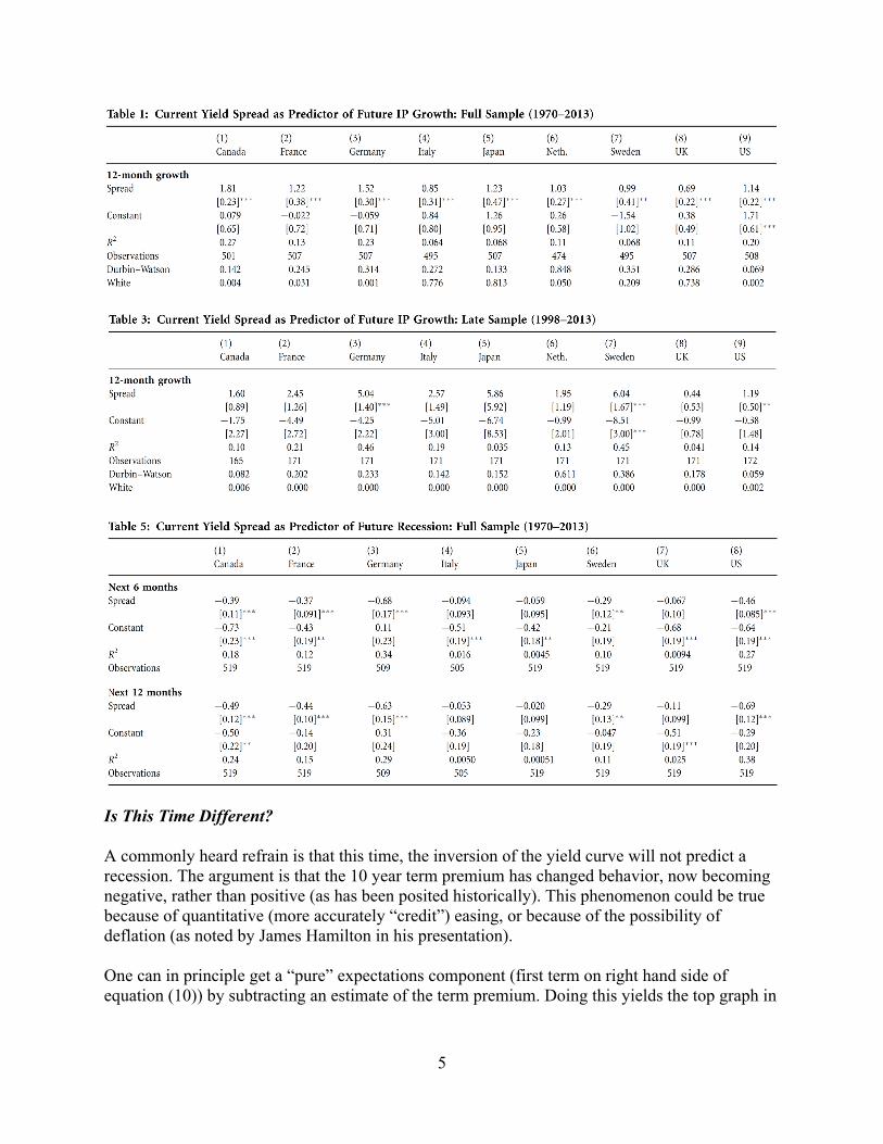
The EHTS merely posits that the yield on a long-term bond is the average of the one period interest rates expected over the lifetime of the long bond. The liquidity theory allows that there will be supply and demand conditions that pertain specifically to bonds of that maturity (this is the segmented markets hypothesis). The presence of idiosyncratic effects associated with a certain maturity of bond is sometimes linked to the “preferred habitat theory”, the idea that certain investors have a preference for purchasing assets of specific maturities. Since 𝑡𝑡𝑡𝑡𝑛𝑛𝑡𝑡 > 0 and is expected to rise as n becomes large, the yield curve will slope upward when short rates are expected to be constant over time. The liquidity or term premium is assumed to rise with maturity n because holders of longer term bonds face greater interest rate and inflation risk. Now, for the sake of simplicity, consider the case where 𝑡𝑡𝑡𝑡𝑛𝑛𝑡𝑡 = 0 (i.e., the EHTS explains all variation in long rates). Suppose further expected short rates are lower than the short rate today. Then the long rate will be lower than the short rate (i.e., the yield curve inverts). Since low interest rates are typically associated with decreased economic activity, an inverted yield curve should imply an expected downturn, especially given that 𝑡𝑡𝑡𝑡𝑛𝑛𝑡𝑡 > 0, then an inversion should imply a downturn, even more strongly. Application to the United States One of the implications of the EHTS is that expectations of a sequence of low short term rates in the near future will result in the long rate being lower than usual. Short term interest rates are typically low when the economy has encountered a slowdown, or has entered in a recession. At the same time, many recessions have been triggered by increases in the short term policy rate (the Fed funds rate). Hence, it is often thought that an inversion of the yield curve presages a recession. In Figure 1, I plot three Treasury yields: (i) 10 year, (ii) 2 year, (iii) 3 month. Those

3

are used to generate two spreads, shown in Figure 2: the 10 year-3 month spread, and the 10 year-2 year spread.

0

4

8

12

16

20

60 65 70 75 80 85 90 95 00 05 10 15 20

Treasuryyields, %

3 month

2 year

10 year

Figure 1: Ten year (black), two year (red), and three month (blue) Treasury yields, % NBER defined recession dates shaded gray. Source: St. Louis Fed FRED, and NBER.

-3

-2

-1

0

1

2

3

4

5

60 65 70 75 80 85 90 95 00 05 10 15 20

Treasuryterm spreads, %

10 yr - 3 mo

10 yr - 2 yr

Figure 2: Ten year-three month spread (blue), and ten year-two year spread (red). NBER defined recession dates shaded gray. Source: St. Louis Fed FRED, and NBER.

4

Notice that inversions of the yield curves (when the lines dip below zero, or come close is) often precede recession. There is a large literature which tries to assess whether the relationship between the yield curve and subsequent economic activity (either growth or recession) is robust. A separate, but related, question whether the term premium provides additional information above and beyond that provided by lagged income and other indicators. A general reading of the literature is the yield curve did have some predictive power, but was declining over time. Wright (2006) argued that the level (namely, the level of the short term interest rate) as well as the slope of the yield curve needed to be included. Cross-country Analysis The evidence for predictive power across other countries is less developed; see Chinn and Kucko (2015) for discussion. The graphs analogous to Figure 1, for European countries and Japan. These are reproductions of Figure 1 from Chinn and Kucko (2015). The graphs are suggestive, but do not confirm the posited relationships. This is why we need regression analysis.

5

Is This Time Different? A commonly heard refrain is that this time, the inversion of the yield curve will not predict a recession. The argument is that the 10 year term premium has changed behavior, now becoming negative, rather than positive (as has been posited historically). This phenomenon could be true because of quantitative (more accurately “credit”) easing, or because of the possibility of deflation (as noted by James Hamilton in his presentation). One can in principle get a “pure” expectations component (first term on right hand side of equation (10)) by subtracting an estimate of the term premium. Doing this yields the top graph in

6

Figure 3 below (the bottom graph is the estimate of 𝑡𝑡𝑡𝑡10𝑡𝑡 from the NY Fed, based on the methodology of Adrian, Crump and Moench (2013)).

-6

-5

-4

-3

-2

-1

0

1

2

60 65 70 75 80 85 90 95 00 05 10 15 20

Premia adjustedterm spreads, %[NY Fed estimates]

10 yr - 3 mo

10 yr - 2 yr

-1

0

1

2

3

4

5

60 65 70 75 80 85 90 95 00 05 10 15 20

10 year term premium, %[NY Fed estimates]

Figure 3: Top graph: Ten year-three month spread adjusted by estimated ten year term premium. Bottom graph: Ten year estimated term premium. NBER defined recession dates shaded gray. Source: St. Louis Fed FRED, NBER, and NY Fed. Notice inversions of the 10yr-3mo premium adjusted term spread are not necessarily always precursors of a recession. Through the 1980s and mid-1990’s, the adjusted spread is negative and

7

no recession follows. Moreover, the adjusted spread did not invert prior to the current ongoing recession. However, there are different estimates of the term premium, and as noted by Chinn (2019), different adjustments lead to different implied probabilities of recession. Using the SF Fed estimate would yield a higher probability of recession than using the NY Fed’s estimate. References

Adrian, Tobias, Richard K. Crump, and Emanuel Moench, “Pricing the Term Structure with Linear Regressions,” Journal of Financial Economics 110, no. 1 (October 2013): 110-38 Chinn, Menzie, “An Ad Hoc Term Premium Adjusted Term Spread Model,” Econbrowser, August 25, 2019. http://econbrowser.com/archives/2019/08/an-ad-hoc-term-premium-adjusted-term-spread-recession-model Chinn, Menzie and Kavan Kucko, “The Predictive Power of the Yield Curve across Countries and Time,” International Finance, 18(2): 129–262 (Summer 2015). Wright, Jonathan, “The Yield Curve and Predicting Recessions,” Finance and Economic Discussion Series No. 2006-07, Federal Reserve Board, 2006. e435_ehts_f21 10.2.2021