Extracting Firms' Short-Term Inflation Expectations from the Economy Watchers Survey Using Text Analysis

Jouchi Nakajima* jouchi.nakajima@boj.or.jp

Hiroaki Yamagata* hiroaki.yamagata@boj.or.jp

Tatsushi Okuda** tatsushi.okuda@boj.or.jp

Shinnosuke Katsuki*** shinnosuke.katsuki@boj.or.jp

Takeshi Shinohara*** takeshi.shinohara@boj.or.jp

No.21-E-12 October 2021

Bank of Japan 2-1-1 Nihonbashi-Hongokucho, Chuo-ku, Tokyo 103-0021, Japan

* Research and Statistics Department ** Research and Statistics Department (currently at the Financial System and Bank

Examination Department) ***

Research and Statistics Department (currently at the Institute for Monetary and

Economic Studies)

Papers in the Bank of Japan Working Paper Series are circulated in order to stimulate discussion and comments. Views expressed are those of authors and do not necessarily reflect those of the Bank. If you have any comment or question on the working paper series, please contact each author. When making a copy or reproduction of the content for commercial purposes, please contact the Public Relations Department (post.prd8@boj.or.jp) at the Bank in advance to request permission. When making a copy or reproduction, the source, Bank of Japan Working Paper Series, should explicitly be credited.

Bank of Japan Working Paper Series

Extracting Firms' Short-Term Inflation Expectations from the Economy Watchers Survey Using Text Analysis*

Jouchi Nakajima† Hiroaki Yamagata‡ Tatsushi Okuda§

Shinnosuke Katsuki

# Takeshi Shinohara

October 2021

Abstract

This paper discusses the Price Sentiment Index (PSI), a quantitative indicator of firms' outlook for general prices proposed by Otaka and Kan (2018). The PSI is developed from the textual data of the Economy Watchers Survey conducted by the Cabinet Office; it is computed by extracting firms' views from survey comments, using text analysis. In this paper, we revisit the PSI and quantitatively analyze the determinants of changes in the PSI and the relationship between the PSI and macroeconomic variables. We also address a shortcoming in the text analysis used for computing the PSI that we discover when examining the performance of the PSI since the COVID-19 outbreak. The results of our analyses show that the PSI tends to precede consumer prices by several months and that it reflects various factors affecting price developments, including demand factors associated with the business cycle and cost factors such as changes in raw materials prices and exchange rates. Our analysis suggests that the PSI is a useful monthly indicator of inflation expectations, in that it captures the price-setting stance of firms responding to the Economy Watchers Survey. While the PSI is subject to large short-term fluctuations, it can be used to complement other indicators used for the analysis of price developments such as the output gap, existing indicators of inflation expectations, and anecdotal information from various sources.

JEL classification: C53, C55, E31, E37. Keywords: Inflation Expectations, Machine Learning, Text Analysis, Big Data.

* The authors thank Kosuke Aoki, Ryo Jinnai, Seisaku Kameda, Kazushige Kamiyama, Takuji Kawamoto, Ichiro Muto, Takashi Nagahata, Teppei Nagano, Koji Nakamura, Koji Takahashi, and staff members of the Bank of Japan for their valuable comments. The authors are also grateful to Rina Matsukura for assistance. Any remaining errors are our own. The views expressed in this paper are those of the authors and do not necessarily reflect the official views of the Bank of Japan. † Research and Statistics Department, Bank of Japan. E-mail: jouchi.nakajima@boj.or.jp. ‡ Research and Statistics Department, Bank of Japan. E-mail: hiroaki.yamagata@boj.or.jp. § Research and Statistics Department (currently at the Financial System and Bank Examination Department),

Bank of Japan. E-mail: tatsushi.okuda@boj.or.jp. # Research and Statistics Department (currently at the Institute for Monetary and Economic Studies), Bank

of Japan. E-mail: shinnosuke.katsuki@boj.or.jp. Research and Statistics Department (currently at the Institute for Monetary and Economic Studies), Bank

of Japan. E-mail: takeshi.shinohara@boj.or.jp.

1

1. Introduction

Inflation expectations are a key variable affecting macroeconomic outcomes and in recent

years have attracted attention in both theoretical and empirical research. Significant progress

has been made in the study of households' and market participants' inflation expectations,

reflecting the accumulation of related data. On the other hand, there has been relatively little

progress in the study of firms' inflation expectations, partly reflecting the paucity of relevant

data. Firms are price setters and their inflation expectations are conventionally regarded as

a critical variable that affects price developments by shifting the Phillips curve. Some recent

studies suggest that firms form their inflation expectations through a different mechanism

than households and investors.1 Meanwhile, some central banks have been conducting

surveys to capture firms' inflation expectations and/or have econometrically estimated the

contribution of inflation expectations to macroeconomic fluctuations.2

In Japan, developments in firms' inflation expectations have primarily been tracked by

the forecast diffusion index (DI) for changes in output prices and the inflation outlook of

enterprises (one, three, and five years ahead) in the Bank of Japan's Tankan (Short-Term

Economic Survey of Enterprises in Japan). Of these, the forecast DI for changes in output

prices has been compiled for decades, thus providing long-term times series data that have

long been used to monitor firms' inflation expectations. Another indicator of firms' inflation

expectations is the Price Sentiment Index (PSI) proposed by Otaka and Kan (2018) in the

Bank of Japan Working Paper Series. The PSI is a quantitative indicator of firms' views

regarding the outlook for prices extracted from respondents' comments in the Economy

Watchers Survey (EWS, hereafter) conducted by the Cabinet Office, using text analysis.

The PSI has the following advantages. First, it is timely, since the EWS is a monthly

survey and its results are released early in the following month. Second, the PSI can be

computed back to January 2000, meaning that it provides sufficiently long time series data

to allow for quantitative analyses. Third, the PSI reflects the views of EWS respondents,

who hold jobs that enable them to closely watch developments in economic activity, in

particular, of households. Fourth, the PSI tends to lead consumer prices by several months.

1 See, for example, Kumar et al. (2015), Coibion, Gorodnichenko, and Kamdar (2018), and Coibion, Gorodnichenko, and Kumar (2018). Studies examining Japanese firms' inflation expectations include Uno et al. (2018a,b), Inatsugu et al. (2019), and Kitamura and Tanaka (2019). 2 In the United States, the Federal Reserve Bank of Atlanta began conducting the Business Inflation Expectations survey in 2011, which surveys businesses managers. Examples of long-standing surveys asking firms for their expectations of the economy are the Survey of Expectations conducted by the Reserve Bank of New Zealand since 1987 and the Business Outlook Survey conducted by the Bank of Canada since 1997.

2

On the other hand, much remains to be examined regarding the PSI, including the

determinants of fluctuations in the PSI, the link with macroeconomic variables, and its

usefulness in forecasting consumer prices. Moreover, since the start of 2020, new terms such

as "COVID-19" and "'Go To' campaign" have emerged and increased significantly in EWS

respondents' comments amid the spread of COVID-19.3 This raises the possibility that the

PSI since then does not sufficiently capture future developments in prices. Based on these

considerations, this paper highlights a shortcoming in the PSI computed based on the current

method and addresses this shortcoming by revising the computation method. Further, it

quantitatively examines the determinants of fluctuations in the PSI and the link between the

PSI and macroeconomic variables.

The remainder of the paper is organized as follows. Section 2 explains how the PSI is

computed using text analysis, examines developments in the PSI, and details the

aforementioned shortcoming in the PSI computed based on the current method. Section 3

seeks to address the shortcoming by revising the way the PSI is computed. Section 4 analyzes

the causes of changes in the PSI and the relationship between the PSI and macroeconomic

variables. Section 5 concludes.

2. Methodology to compute the PSI using text analysis

2.1. The Economy Watchers Survey (EWS)

The EWS has been conducted monthly by the Cabinet Office since January 2000. The survey

aims to grasp developments in Japan's economy in a timely manner. Each month, 2,050

people across Japan receive the survey and about 1,800 of them provide valid responses.4

Survey respondents consist of "economy watchers," that is, individuals holding jobs that

enable them to closely watch developments in economic activity: for example, business

managers and grocery clerks. Figure 1 shows the composition of EWS respondents by

industry and region. Figure 1(a) indicates that those engaged in household activity-related

sectors account for about two thirds of respondents, while those working in corporate

activity-related and employment-related sectors account for around 20 percent and 10

percent, respectively. This means that many of the survey respondents are engaged in

industries that have a relatively close link with consumers. Meanwhile, Figure 1(b) shows

that the regional distribution of survey respondents is well balanced, with respondents

3 Note that the terms we use to refer to comments in the EWS are our translations of the comments in the Japanese original. 4 In this paper, we use the PSI from 2001 onward for econometric analyses as the number of responses in 2000, the year the survey was started, is considerably smaller than from 2001 onward.

3

representing all the major regions across Japan, from Hokkaido to Okinawa.

The headline results from the EWS are the DIs for current and future economic

conditions, presented in Figure 2. They are calculated using each respondent's assessment of

current or future economic conditions on a scale comprising five categories ranging from,

e.g., "better" to "worse." The DI for current economic conditions has been regarded as a

timely and useful indicator for assessing economic activity, as it shows some correlation with

other macroeconomic indicators that capture economic developments.

The EWS is unique in that it collects not only respondents' assessment of economic

conditions on a scale as just described but also their comments giving reasons for their

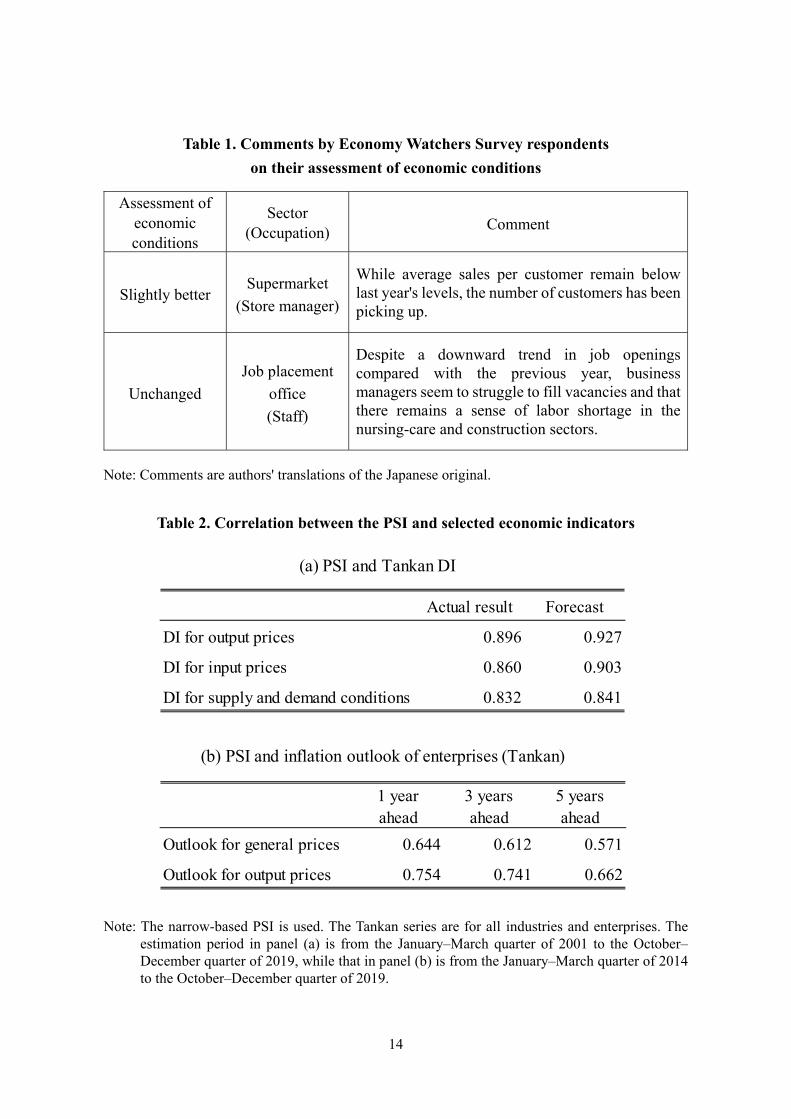
assessment. Examples of such comments are provided in Table 1. On average, approximately

1,100 of the about 1,800 respondents in each survey provide comments on their economic

assessments. These comments are organized and released as textual data on the Cabinet

Office's website.5 Such data in the release for each survey consist of about 100,000 words

in total and around 3,000 unique words, and can therefore be regarded as big data. The PSI

is derived from this big textual data and is computed by extracting and quantifying

information regarding price developments from the data, using text analysis.6 The specific

methods for computing the PSI are presented in the next subsection.

2.2. Computing method for the PSI

When respondents provide comments giving the reasons for their economic assessments in

the EWS, they sometimes also refer to consumers' spending stance and to developments in

prices such as commodity prices. The PSI is designed to capture developments in the

difference between the share of comments implying inflation and the share of comments

implying deflation by classifying comments.

Specifically, survey comments are classified into the following four types:

A. Comments implying inflation

B. Comments implying deflation

C. Comments implying zero inflation (neither inflation nor deflation)

D. Comments not referring to price developments

Manually screening the over 1,000 comments received in each survey to classify them into

these four types would require considerable time and effort. Moreover, such manual

5 Note that the textual data we mention here is in Japanese. 6 An example of a study analyzing the textual data of the EWS is that by Goshima et al. (2021).

4

classification could result in incorporating the analysts' subjective views into the PSI.

Therefore, for computing the PSI, comments are automatically classified into the four types

based on the terms contained in each comment. This is done using machine learning.

Specifically, before the automatic classification, selected terms are assigned scores

indicating to which type a comment containing the term is likely to belong. The procedure

starts by randomly extracting 1,500 sample comments from the EWS during the period

2001–2017. Each of these comments is then manually examined and classified into one of

the four types (A to D). This process is essential for the text analysis to compute the PSI,

although it leaves some room for analysts' subjective views to be incorporated into the index.

To minimize such potential bias to the greatest extent possible, in this process, comments in

which respondents' views on price developments appear to be ambiguous are classified as

type D.

The sample comments and their classification results are then used as supervised

training data to train the machine learning algorithm. This is shown as Step 1 in Figure 3,

which provides an illustration of the procedure used for computing the PSI. In this step, the

training data and the Naïve Bayes classifier are used to estimate scores for the terms in the

sample comments. Specifically, each sample comment is inputted into the classifier so as to

obtain the optimal term scores yielding the "correct" output, that is, the same classification

result as that obtained from the manual classification. A key variable in the estimation is the

relative frequency with which a term appears in each type of comment A to D. For example,

if the term "pass on" appears more frequently in comments implying inflation (type A) than

in comments implying deflation (type B), this means that the score of "pass on" for type A

is larger than that for type B. Given this, term scores can be interpreted as measures gauging

the marginal increase in the likelihood of a comment being classified as a certain type if the

comment contains the term.7

Using the estimated term scores, comments from each survey are classified into types

A to D. In Figure 3, this is shown as Step 2, where comments are classified into the type that

received the highest score based on the terms contained in the comment. Finally, for each

survey, the PSI is calculated as the share of comments implying inflation (type A) minus the

share of comments implying deflation (type B). Specifically, the PSI is defined as follows:

7 It should be noted that the score also depends on the number of comments classified into each type in the manual classification. For a detailed description of the Naïve Bayes classifier, see, for example, Murphy (2012).

5

PSI Number of type A comments Number of type B comments

Total number of type A, B, and C comments

In the remainder of this paper, we use the PSI data normalized by the mean and standard

deviation for the period 2000–2019. While the PSI is computed separately for comments on

current economic conditions and on future economic conditions, the following analyses use

the PSI based on comments on current economic conditions. We also conducted the analyses

using the PSI based on comments on future economic conditions and found that results do

not change significantly.

2.3. Developments in the PSI

In this subsection, we examine developments in the PSI computed using the method

described in the previous subsection (we will refer to this as the broad-based PSI hereafter).

As shown in Figure 4(a), developments in the broad-based PSI clearly differ from those in

the current economic conditions DI. For example, around 2007–2008, when commodity

prices were surging, the current economic conditions DI declined due to concerns over a

decrease in profits, whereas the broad-based PSI rose, clearly reflecting the rise in raw

materials prices. Around 2008–2009, on the other hand, the broad-based PSI fell

substantially in tandem with the current economic conditions DI amid the significant decline

in demand both at home and abroad due to the impact of the global financial crisis. These

findings suggest that developments in the PSI are significantly affected by changes in

demand due to the business cycle and also by cost factors such as commodity price changes.

Figure 4(b) presents developments in the PSI and the year-on-year rate of change in the

consumer price index (CPI, all items less fresh food and energy). As can be seen in the figure,

developments in the PSI appear to somewhat precede those in the CPI inflation rate. This

visual impression is confirmed when we estimate simple lead-lag correlation coefficients

between the two indexes for the period through the end of 2019.We find that the correlation

coefficient between the PSI and the seasonally adjusted quarter-on-quarter rate of change in

the CPI is largest – taking a value of 0.54 – when the PSI leads the CPI inflation rate by one

month. We further find that the correlation coefficient between the PSI and the year-on-year

rate of change in the CPI is largest – taking a value of 0.76 – when the PSI leads the CPI

inflation rate by seven months.

However, from the start of 2020, this relationship between the broad-based PSI and the

CPI appears to break down. Unlike the CPI inflation rate, the PSI registered a relatively

substantial rise during the COVID-19 pandemic. This seems to be largely due to the fact that

since the PSI was originally developed in 2018, new terms such as "COVID-19" and "'Go

6

To' campaign" have emerged and increased in number in the EWS comments. Although

terms such as "virus" and "campaign" appeared in survey comments collected before the

COVID-19 outbreak, the sense in which they were used partly differs from that since the

COVID-19 pandemic.

This matters because of the scores assigned to the terms for computing the broad-based

PSI. For instance, "virus" was assigned a relatively high score for type A price changes

(pointing to inflation). This means that the rise in the PSI during the pandemic partly reflects

the increase in the number of comments referring to the "coronavirus." The term "campaign"

was also assigned a high score for type A price changes, meaning that mentions of the "'Go

To' campaign" push up the PSI. Given that the term scores are based on data prior to the

outbreak of COVID-19, they may not sufficiently reflect price conditions today under the

pandemic. For example, while a discount on hotel charges through the "Go To Travel"

campaign directly pushes down consumer prices in the short run, mentions of the term

"campaign" push up the broad-based PSI, pointing to inflation, due to the scores assigned to

the term based on pre-pandemic textual data.

Examining developments in the broad-based PSI, we find that the PSI may not

sufficiently capture future price developments when the use of new terms increases

significantly. Therefore, the pandemic has revealed a shortcoming in the text analysis used

for computing the PSI. To address this shortcoming, we revise the computation method for

the PSI.8

3. Revision of the computation method for the PSI

3.1. Methodology

The broad-based PSI is based on around 3,000 terms that are assigned scores. We find that

the relationship of some of these terms with the direction of prices is unclear, and that others

appear in the comments only for a certain period. When the PSI is significantly affected by

such terms, the change in the index can be difficult to interpret and the relationship between

the PSI and the underlying trend in prices may break down.

To improve the PSI, we narrow down the list of 3,000 terms to those satisfying the

following criteria: terms (1) that on average appear at least five times a month during the

8 As one potential approach to revising the computation method for the PSI, we considered simply extending the period used for extracting sample comments to incorporate data up to the most recent month for which data are available. However, we found that currently the number of observations is too small to link new terms such as "COVID-19" with a particular direction of prices, so that we need to wait for more data to become available.

7

period 2001–2019, (2) that can be regarded as indicating a clear direction in prices and

economic activity, and (3) whose number of appearance is correlated with the actual inflation

rate in that the sign of that correlation matches the direction of prices and economic activity

with which one would associate the term. For example, the term "sale" meets criterion (1),

but the term "campaign" does not because it only appears in the comments for a certain

period. While criterion (2) involves some judgement in the selection of terms, we find that

there are terms that clearly imply the direction of prices, such as "raising prices," and terms

that do not necessarily suggest such direction, such as "unit price." Finally, an illustration of

criterion (3) is that, a priori, one would expect the correlation between the CPI inflation rate

and the number of times the term "rise" appears to be positive.

Among the terms satisfying the above criteria, we search the combination of terms that

yields the highest correlation coefficient with the year-on-year rate of change in the CPI (all

items less fresh food and energy). Using this optimization process, we obtain 20 terms to

compute a new PSI.9 Having referred to the PSI developed based on the original method as

the broad-based PSI, we call the PSI built using these 20 terms the narrow-based PSI.

3.2. Developments in the narrow-based PSI

Next, we compare developments in the narrow-based PSI with those in the broad-based PSI.

As shown in Figure 4(b), developments in the narrow-based PSI are generally similar to

those in the broad-based PSI for the period through the end of 2019. However, unlike the

broad-based PSI, which rose in early 2020, the narrow-based PSI declined in the March‒

May period and since then, despite some fluctuations, has been around the same level as in

2019. To investigate the link between the broad- and the narrow-based PSI on the one hand

and the CPI inflation rate on the other, we calculate the lead-lag coefficients for the period

from January 2010 through December 2020. In terms of the correlation with the year-on-

year rate of change in the CPI for all items less fresh food and energy, the largest coefficient

we obtain for the broad-based PSI is 0.75 (when it leads the CPI by 8 months), while the

largest coefficient for the narrow-based PSI is 0.80 (when it leads the CPI by 10 months). In

terms of the correlation with the year-on-year rate of change in the CPI for all items less

fresh food (i.e., including energy), the largest coefficient for the broad-based PSI is 0.61

(when it leads the CPI by 3 months), while the largest coefficient for the narrow-based PSI

9 The selected terms are as follows: rise; good; high; exceed; price increase; raising prices; surge; stable; decline; bad; cheap; low; price cut; fall; sluggish; deteriorate; decrease; severe; competition; and sale. We note that we end up with the same set of terms when we search the combination of terms that yields the largest correlation coefficient vis-à-vis the year-on-year rate of change in the CPI for all items less fresh food (i.e., including energy).

8

is 0.71 (when it leads the CPI by 3 months). Therefore, in both cases, the largest coefficient

for the narrow-based PSI is larger than the largest coefficient for the broad-based PSI.

These findings suggest that the narrow-based PSI provides a better indicator which

robustly tends to lead the CPI than the broad-based PSI when the economy and prices enter

a new phase and the use of new terms increases in the EWS comments. That said, since the

number of terms on which the narrow-based PSI is based is limited to 20, it potentially fails

to incorporate the implications of a number of comments that are covered by the broad-based

PSI. In sum, both the broad-based and narrow-based PSIs have advantages and

disadvantages depending on the circumstances. Therefore, from a practical perspective,

monitoring developments in both PSIs is desirable.

In what follows, we quantitatively analyze the empirical properties of the narrow-based

PSI. We note that conducting the same analysis for the broad-based PSI yields qualitatively

similar results.

4. The PSI as a proxy for short-term inflation expectations

4.1. The link between the PSI and economic indicators

Figure 5 presents developments in the PSI and in the Tankan DIs for all industries and

enterprises. We find that the PSI has a high correlation with the DIs for output prices, for

input prices, and for domestic supply and demand conditions. This suggests that the PSI

reflects not only firms' price-setting behavior but also firms' perceptions of their demand

conditions and input costs. Table 2(a) shows that the correlation coefficients between the PSI

and these Tankan DIs, at over 0.8, are high, and that the coefficients are all – albeit slightly

– higher for the forecast DI (one quarter ahead) than for the actual DI. This suggests that the

PSI provides a useful proxy for short-term inflation expectations that captures firms' price-

setting stance for the period ahead rather than their present price-setting stance. This is also

consistent with the earlier finding that the PSI somewhat leads the inflation rate. Figure 6

and Table 2(b) provide further support: they suggest that the PSI shows some correlation

with firms' one-year-ahead outlook for both general prices and output prices reported in the

Tankan. These findings suggest that the PSI is closely linked with macroeconomic variables

that affect price developments.

4.2. The link between the PSI and consumer prices

In this subsection, we examine whether the PSI provides unique information such that it

complements information on the output gap and other conventional macroeconomic

9

variables for the forecasting of inflation. Specifically, we conduct regression analyses using

the one-quarter-ahead inflation rate as the dependent variable. In this analysis, we first

estimate a regression equation using the exchange rate and the output gap as independent

variables. We then add the PSI as an independent variable to the equation and examine how

the regression results change as a result. The inflation rate is measured in terms of the year-

on-year rate of change in the CPI (all items less fresh food and energy, excluding the effects

of the consumption tax hikes), while for the exchange rate the year-on-year rate of change

in the nominal effective exchange rate is used. The output gap is estimated by the Bank of

Japan's Research and Statistics Department. The estimation period for the regression is from

the January‒March quarter of 2001 to the October‒December quarter of 2019.

The regression results are shown in Table 3. In the specification without the PSI, the

coefficients on the exchange rate and the output gap are statistically significant. When the

PSI is added, these coefficients remain statistically significant and the coefficient on the PSI

is also significant. We further find that the explanatory power in terms of the adjusted R-

squared is higher when the PSI is included. These results suggest that the PSI appears to

capture additional information relevant for changes in the inflation rate not captured by the

output gap and the exchange rate. It should be noted that we obtain similar results when

adding crude oil prices as an independent variable or replacing the exchange rate with import

prices.

Next, we employ a vector autoregression (VAR) model to examine the relationship

between the PSI and macroeconomic variables including the inflation rate. In this estimation,

we use four variables: the nominal effective exchange rate (quarter-on-quarter change); the

output gap; the PSI; and the CPI (all items less fresh food and energy; seasonally adjusted

quarter-on-quarter change). We identify shocks using Cholesky decomposition, with the

variables ordered as above.10 The estimation period is from the January‒March quarter of

2001 to the October‒December quarter of 2019. Based on the Akaike information criterion

(AIC), the lag length is set to two quarters.

Figure 7 shows the impulse responses of the VAR model. Figure 7(a) indicates that the

responses of the PSI to an exchange rate shock and an output gap shock are statistically

10 The variables are ordered from the most exogenous to the least exogenous one. This reflects our assumptions regarding the nature of the quarterly shock to each variable. Specifically, we assume that, during the same quarter, (1) an exchange rate shock may affect all the other variables, (2) an output gap shock may influence firms' inflation expectations (the PSI) and the actual inflation rate (the CPI), and (3) a PSI shock may have an impact on the CPI. A shock to the CPI here is assumed to have no impact on the PSI during the same quarter. It should be noted that even if we change the order of the PSI and the CPI by assuming that a CPI shock in this ordering may affect the PSI during the same quarter, we obtain qualitatively the same impulse responses of the variables as presented below.

10

significant. The PSI reacts to an exchange rate shock almost contemporaneously and to an

output gap shock with a lag of about 3–4 quarters. This implies that the PSI is closely related

to the macroeconomic variables which affect the inflation rate.

Turning to Figure 7(b), we further find that the response of the inflation rate to a PSI-

specific shock is statistically significant. It is noteworthy that the inflation rate reacts to a

PSI-specific shock with a lag of about 1–2 quarters, indicating that the PSI tends to lead the

inflation rate. These results suggest that the PSI contains unique information regarding future

changes in the inflation rate not captured by the exchange rate and the output gap.

Using the regression model, we now test the predictive power of the PSI for the inflation

rate (i.e., the year-on-year rate of change in the CPI for all items less fresh food and energy).

Specifically, we conduct one-quarter-ahead forecasting of the inflation rate for each quarter

from the January‒March quarter of 2012 to the October‒December quarter of 2019. We start

the test by estimating the regression equation using the data for the period through the

October‒December quarter of 2011 and then predict the inflation rate for the January‒March

quarter of 2012. Next, we estimate the regression equation again using the data for the period

through the January‒March quarter of 2012 and then forecast the inflation rate for the April‒

June quarter of 2012. By repeating this out-of-sample forecasting for each quarter, we obtain

the predicted inflation rates for the period through the October‒December quarter of 2019.

Finally, we measure the accuracy of these out-of-sample forecasts by calculating the root-

mean-squared error (RMSE) between the forecasts and the actual inflation rates. The bottom

row of Table 3 shows the results of this forecasting exercise, which indicate that the RMSE

of the specification including the PSI is about 10 percent smaller than that of the specification

without the PSI.

In sum, the analyses reveal that the PSI provides additional information on changes in

consumer prices over the next several months not captured by such macroeconomic variables

as exchange rates and the output gap. Computed from comments by respondents to the EWS,

i.e., individuals holding jobs that enable them to closely watch developments in economic

activity, the PSI thus appears to be a useful proxy for firms' short-term inflation

expectations.11

11 Among studies using text analysis to examine inflation expectations, Guzman (2011) develops an indicator of U.S. inflation expectations using the number of Google search queries, while Angelico et al. (2021) construct an indicator of Italian inflation expectations using textual data from Twitter. Studies predicting the CPI inflation rate using text analysis include Seabold and Coppola (2015), Wei et al. (2017), and Goshima et al. (2021).

11

5. Concluding remarks

This paper focused on the Price Sentiment Index (PSI), a quantitative indicator of firms'

outlook for general prices computed from comments provided by respondents to the

Economy Watchers Survey, using text analysis. We provide empirical evidence that the PSI

is a useful indicator of firms' short-term inflation expectations. Our analyses suggest that the

PSI reflects demand factors associated with the business cycle and cost factors such as

changes in raw materials prices and in exchange rates. While the PSI is subject to large short-

term fluctuations, it does appear to be useful in capturing, on a monthly basis, the price-

setting stance of firms responding to the Economy Watchers Survey. Overall, the analysis

suggests that the PSI is a useful indicator to supplement existing measures for monitoring

developments in inflation expectations such as the output gap, existing indicators of inflation

expectations, and anecdotal information.

12

References

Angelico, Cristina, Juri Marcucci, Marcello Miccoli, and Filippo Quarta (2021). "Can we

measure inflation expectations using Twitter?" Bank of Italy Working Papers, No. 1318.

Coibion, Oliver, Yuriy Gorodnichenko, and Rupal Kamdar (2018). "The formation of

expectations, inflation, and the Phillips curve," Journal of Economic Literature, 56(4),

pp. 1447‒1491.

Coibion, Olivier, Yuriy Gorodnichenko, and Saten Kumar (2018). "How do firms form their expectations? New survey evidence," American Economic Review, 108(9), pp.

2671‒2713.

Goshima, Keiichi, Hiroshi Ishijima, Mototsugu Shintani, and Hiroki Yamamoto (2021).

"Forecasting Japanese inflation with a news-based leading indicator of economic

activities," Studies in Nonlinear Dynamics & Econometrics, 25(4), pp. 111–113.

Guzman, Giselle (2011). "Internet search behavior as an economic forecasting tool: The case

of inflation expectations," Journal of Economic and Social Measurement, 36(3), pp. 119‒

167.

Inatsugu, Haruhiko, Tomiyuki Kitamura, and Taichi Matsuda (2019). "The formation of

firms' inflation expectations: A survey data analysis," Bank of Japan Working Paper

Series, No. 19-E-15.

Kitamura, Tomiyuki, and Masaki Tanaka (2019). "Firms' inflation expectations under

rational inattention and sticky information: An analysis with a small-scale

macroeconomic model," Bank of Japan Working Paper Series, No. 19-E-16.

Kumar, Saten, Hassan Afrouzi, Olivier Coibion, and Yuriy Gorodnichenko (2015). "Inflation

targeting does not anchor inflation expectations: Evidence from firms in New Zealand,"

Brookings Papers on Economic Activity, 2015(2), pp. 151‒225.

Murphy, Kevin (2012). Machine Learning: A Probabilistic Perspective, MIT Press.

Otaka, Kazuki, and Kazutoshi Kan (2018). "Economic analysis using machine learning: Text

mining of the 'Economy Watchers Survey'," Bank of Japan Working Paper Series, No.

18-J-8 (in Japanese).

Seabold, Skipper, and Andrea Coppola (2015). "Nowcasting prices using Google trends: An

application to Central America," Policy Research Working Paper, No. 7398, World Bank.

13

Uno, Yosuke, Saori Naganuma, and Naoko Hara (2018a). "New facts about firms' inflation

expectations: Simple tests for a sticky information model," Bank of Japan Working Paper

Series, No. 18-E-14.

Uno, Yosuke, Saori Naganuma, and Naoko Hara (2018b), "New facts about firms' inflation

expectations: Short- versus long-term inflation expectations," Bank of Japan Working

Paper Series, No. 18-E-15.

Wei, Yunjie, Xun Zhang, and Shouyang Wang (2017). "Can search data help forecast

inflation? Evidence from a 13-country panel," Proceedings, 2017 IEEE International

Conference on Big Data.

14

Table 1. Comments by Economy Watchers Survey respondents

on their assessment of economic conditions

Assessment of economic conditions

Sector (Occupation) Comment

Slightly better Supermarket

(Store manager)

While average sales per customer remain below last year's levels, the number of customers has been picking up.

Unchanged

Job placement

office

(Staff)

Despite a downward trend in job openings compared with the previous year, business managers seem to struggle to fill vacancies and that there remains a sense of labor shortage in the nursing-care and construction sectors.

Note: Comments are authors' translations of the Japanese original.

Table 2. Correlation between the PSI and selected economic indicators

Note: The narrow-based PSI is used. The Tankan series are for all industries and enterprises. The estimation period in panel (a) is from the January‒March quarter of 2001 to the October‒December quarter of 2019, while that in panel (b) is from the January‒March quarter of 2014 to the October‒December quarter of 2019.

Actual result Forecast

DI for output prices 0.896 0.927

DI for input prices 0.860 0.903

DI for supply and demand conditions 0.832 0.841

(a) PSI and Tankan DI

1 yearahead

3 yearsahead

5 yearsahead

Outlook for general prices 0.644 0.612 0.571

Outlook for output prices 0.754 0.741 0.662

(b) PSI and inflation outlook of enterprises (Tankan)

15

Table 3. Regression results

Note: The narrow-based PSI is used. "CPI (current quarter)" refers to the year-on-year rate of change in the CPI (all items less fresh food and energy, excluding the effects of the consumption tax hikes and policies concerning the provision of free education). "Exchange rate" refers to the year-on-year rate of change in the nominal effective exchange rate. The estimation period is from the January‒March quarter of 2001 to the October‒December quarter of 2019. Figures in parentheses are heteroskedasticity- and autocorrelation-consistent (HAC) standard errors. ***, **, and * denote statistical significance at the 1, 5, and 10 percent levels, respectively. The RMSE is computed to assess the predictive performance of the out-of-sample forecasts from the January‒March quarter of 2012 to the October‒December quarter of 2019.

Independent variables

Constant 0.046 ** 0.016

(0.022) (0.026)

CPI (current quarter) 0.868 *** 0.814 ***

(0.037) (0.047)

Output gap 0.066 *** 0.035 *

(0.024) (0.020)

Exchange rate -0.009 *** -0.007 **

(0.003) (0.003)

PSI 0.099 *

(0.057)

Standard errors

Adjusted R-squared

RMSE

Dependent variable: CPI (1 quarter ahead)

0.914 0.920

0.177 0.162

Not including PSI Including PSI

0.201 0.194

16

Figure 1. Economy Watchers Survey: Composition of survey respondents

Figure 2. Economy Watchers Survey: DIs for current and future economic conditions

Hokkaido, 6.3

Tohoku,9.9

Kanto & Koshinetsu, 26.4

Tokai & Hokuriku,

17.4

Kinki,13.7

Chugoku & Shikoku,

14.2

Kyushu & Okinawa, 12.1

share of respondents, CY 2001‒2020 average, %

(a) By industry

Retail, 39.4

Food and beverage, 4.7

Services, 19.0

Housing, 4.4

Corporate activity-related,

22.3

Employment-related, 10.2

share of respondents, CY 2001‒2020 average, %

Household activity-related, 67.5

(b) By region

5

10

15

20

25

30

35

40

45

50

55

60

65

01 02 03 04 05 06 07 08 09 10 11 12 13 14 15 16 17 18 19 20 21

Current conditions

Future conditions

DI

CY

17

Figure 3. Computation method for the PSI using text analysis

Term scores: "raw materials" Term scores: "pass on"

A B C D A B C D6 2 4 0 7 1 5 1

Total term scores

A B C D85 30 15 4

Comment #1.

... raw materials ... pass on ...

Comment classified as type A

Term scores: "intensify" Term scores: "decline"

A B C D A B C D3 6 3 0 4 8 5 1

Total term scores

A B C D42 70 30 15

Comment #2.

... intensified ... declining ...

Comment classified as type B

A B C D

6 2 4 0

7 1 5 1

3 6 3 0

4 8 5 1

Type A Type B

Type C Type D

…

Sample comments

pass on

intensify

decline

TermType of price change

raw materials

Term scores

Estimated using the Naïve Bayes classifier

Step 1. Estimation of scores for each selected term

Step 2. Classification of comments into types

18

Figure 4. PSI and selected economic indicators

Note: The broad-based PSI is computed using Otaka and Kan's (2018) method, in which about 3,000 terms are assigned scores, while the narrow-based PSI is calculated based on 20 terms. The CPI inflation rate is for all items less fresh food and energy, excluding mobile phone charges and the effects of the consumption tax hikes, policies concerning the provision of free education, and the "Go To Travel" campaign (Bank of Japan's staff estimates).

0

10

20

30

40

50

60

-3

-2

-1

0

1

2

3

01 02 03 04 05 06 07 08 09 10 11 12 13 14 15 16 17 18 19 20 21

PSI (broad based, lhs)

PSI (narrow based, lhs)

DI for current economic conditions (rhs)

index

CY

DI

(a) PSI and DI for current economic conditions

(b) PSI and CPI inflation rate

-3

-2

-1

0

1

2

-3

-2

-1

0

1

2

3

01 02 03 04 05 06 07 08 09 10 11 12 13 14 15 16 17 18 19 20 21

PSI (broad based, lhs)

PSI (narrow based, lhs)

CPI inflation rate (rhs)

index

CY

y/y % chg.

19

Figure 5. PSI and Tankan DIs

Note: The narrow-based PSI is used. The Tankan DIs are for all industries and enterprises.

-50

-40

-30

-20

-10

0

10

20

30

-3

-2

-1

0

1

2

3

4

01 02 03 04 05 06 07 08 09 10 11 12 13 14 15 16 17 18 19 20 21

PSI (lhs)

DI (actual result, rhs)

DI (forecast, rhs)

index

CY

DI

(a) PSI and DI for output prices

-40

-20

0

20

40

60

80

100

-3

-2

-1

0

1

2

3

4

01 02 03 04 05 06 07 08 09 10 11 12 13 14 15 16 17 18 19 20 21

PSI (lhs)DI (actual result, rhs)DI (forecast, rhs)

index

CY

DI

(b) PSI and DI for input prices

-60

-50

-40

-30

-20

-10

0

10

-3

-2

-1

0

1

2

3

4

01 02 03 04 05 06 07 08 09 10 11 12 13 14 15 16 17 18 19 20 21

PSI (lhs)DI (actual result, rhs)DI (forecast, rhs)

index

CY

DI

(c) PSI and DI for supply and demand conditions

20

Figure 6. PSI and 1-year-ahead inflation outlook of enterprises (Tankan)

Note: The narrow-based PSI is used. The Tankan series for the inflation outlook of enterprises are

for all industries and enterprises.

-0.5

0.0

0.5

1.0

1.5

2.0

-1.5

-1.0

-0.5

0.0

0.5

1.0

1.5

2.0

2.5

14 15 16 17 18 19 20 21

PSI (lhs)

Outlook for general prices (rhs)

Outlook for output prices (rhs)

index

CY

%

21

Figure 7. Impulse responses from VAR model

Note: The narrow-based PSI is used. The size of the shock is one standard deviation. The shaded areas indicate the 95 percent confidence intervals. The estimation period is from the January‒March quarter of 2001 to the October‒December quarter of 2019.

-0.5

-0.4

-0.3

-0.2

-0.1

0.0

0.1

0.2

0 2 4 6 8 10

index

-0.2

-0.1

0.0

0.1

0.2

0.3

0.4

0.5

0.6

0 2 4 6 8 10

index

-0.3

0.0

0.3

0.6

0 2 4 6 8 10

index

(a) Impulse responses of the PSI

Exchange rate shock Output gap shock PSI shock

-0.10

-0.08

-0.06

-0.04

-0.02

0.00

0.02

0.04

0 2 4 6 8 10

q/q % chg.

-0.04

-0.02

0.00

0.02

0.04

0.06

0.08

0 2 4 6 8 10

q/q % chg.

-0.04

-0.02

0.00

0.02

0.04

0.06

0.08

0 2 4 6 8 10

q/q % chg.

(b) Impulse responses of the inflation rate

Exchange rate shock Output gap shock PSI shock

quarters

quarters