A Review of Nonlinear Factor Analysis Statistical Methods

Melanie M. Wall, Division of Biostatistics, University of MinnesotaYasuo Amemiya, IBM Thomas J. Watson Research Center

ABSTRACT: Factor analysis that has been used most frequently in practice can be char-acterized as linear analysis. Linear factor analysis explores a linear factor space underlyingmultivariate observations or addresses linear relationships between observations and latentfactors. However, the basic factor analysis concept is valid without this limitation to lin-ear analyses. Hence, it is natural to advance factor analysis beyond the linear restriction,i.e., to consider nonlinear or general factor analysis. In fact, the notion of nonlinear factoranalysis was introduced very early. But, as in the linear case, the development of statisticalmethods lagged that of the concept considerably, and has only recently started to receivebroad attention. This paper reviews such methodological development for nonlinear factoranalysis.

1 Introduction

According to a general interpretation, factor analysis explores, represents, and analyzes a

latent lower dimensional structure underlying multivariate observations, in scienti�c inves-

tigations. In this context, factors are those underlying concepts or variables that de�ne the

lower dimensional structure, or that describe an essential/systematic part of all observed

variables. Then, the use of a model is natural in expressing the lower dimensional structure

or the relationship between observed variables and underlying factors. To de�ne what is a

scienti�cally relevant or interesting essential/systematic structure, the concept of conditional

independence is often used. That is, the underlying factor space explored by factor analysis

has the conditional independence structure where the deviations of observed variables from

the systematic part are mutually unrelated, or where all interrelationships among observed

variables are explained entirely by factors. This interpretation of the factor analysis concept

does not limit the underlying factor space to be a linear space, nor the relationships between

observations and factors to be linear. Hence, the idea of nonlinear factor analysis should not

1

be treated as an extension of the basic factor analysis concept, but should be considered as

an inherent e�ort to make factor analysis more complete and useful.

In the history of factor analysis practice, analysis with a linear structure or a linear

model has been used almost exclusively, and the use of nonlinear analysis has started only

recently. One possible reason for this delay in the use of nonlinear analysis is that, for

many years, the relationships among variables were understood and represented only through

correlations/covariances, i.e., measures of linear dependency. Another reason may be the

technical di�culty in development of statistical methods appropriate for nonlinear or general

factor analysis. The proper model formulation facilitating methodological development has

been part of the di�culty. Considering the fact that appropriate statistical methods for linear

analysis were not established or accepted widely for 60 years, the rather slow development

of statistical methods for nonlinear factor analysis is understandable. This paper is intended

to review such development of nonlinear factor analysis statistical methods.

Since di�erent types of analysis may be interpreted as special cases of nonlinear factor

analysis, it should be helpful to clearly de�ne the scope of this paper. The focus of this paper

is to cover nonlinear factor analysis methods used to explore, model, and analyze relation-

ships or lower dimensional structure that underlies continuous (or treated as such) observed

variables, and that can be represented as a linear or nonlinear function of continuous latent

factors. A type of nonlinearity that is outside of this paper's focus is that dictated by the

discreteness of the observed variables. Factor analysis for binary or polytomous observed

variables has been discussed and used for a number of years. Two popular approaches to

such a situation are the use of threshold modeling and the generalized linear model with a

link function as the conditional distribution of an observed variable given factors. The nature

of nonlinearity in these approaches are necessitated by the observed variable types, and is

2

not concerned with the nonlinearity of the factor space. Another kind of analysis similar to

factor analysis, but not covered here, is the latent class analysis, where the underlying factor

is considered to be unordered categorical. This can be interpreted as a nonlinear factor

structure, but its nature di�ers from this paper's main focus of exploring/modeling under-

lying nonlinear relationships. Another type of nonlinearity occurs in heteroscedastic factor

analysis where the error variances depend on factors, see Lewin-Koh and Amemiya (2003).

Being di�erent from addressing nonlinear relations among variables directly, heteroscedastic

factor analysis is not covered in this paper.

Within this paper's scope with continuous observations and latent variables, one topic

closely related to factor analysis is the structural equation analysis or the so-called LISREL

modeling. As the name LISREL suggests, the models used traditionally in this analysis

have been linear in latent variables. Restricting to linear cases, close relationships exist

between the factor analysis model and the structural equation model (SEM). The factor

analysis can be considered a part of the SEM corresponding to the measurement portion,

or a special case of the SEM with no structural portion. Alternatively, the full SEM can be

considered a special case of the factor analysis model with possible nonlinearity in parame-

ters. But, for methodological research in these two areas, di�erent aspects of analyses tend

to be emphasized. Structural equation analysis methods usually focus on estimation of a

structural model with an equation error with minimal attention to factor space exploration,

and measurement instrument development. For the structural model �tting or estimation, it

is natural to consider models possibly nonlinear in latent variables. Accordingly, a number

of important methodological contributions have occurred in estimation for some types of

nonlinear structural models. The review of this methodological development is included in

this paper (Section 3), although some proposed methods may not be directly relevant for

3

factor analytic interest of exploring nonlinear structure. It should be pointed out that the

special-case relationship between the linear factor analysis model and linear structural equa-

tion model may not extend to the nonlinear case depending on the generality of nonlinear

models being considered. The discussion on this point is also included at the end of Section

3.

Consider the traditional linear factor analysis model for continuous observed and contin-

uous factors,

Zi = �+�fi + �i (1)

where Zi is a p � 1 observable vector for individuals i = 1 : : : n, fi is a q � 1 vector of

\latent" factors for each individual, and the p � 1 vector �i contains measurement error.

The traditional factor analysis model (1) is linear in the parameters (i.e. � and �) and is

linear in the factors. Unlike ordinary regression where the inclusion of functions of observed

variables (e.g. x and x2) would not be considered a nonlinear model as long as the regression

relationship was linear in the coe�cient parameters, with factor analysis, the inclusion of

nonlinear function of the factors will be distinguished as a kind of nonlinear factor analysis

model.

The idea of including nonlinear functions of factors is brie y mentioned in the �rst chapter

of Lawley and Maxwell (1963). While drawing a contrast between principal component and

factor analysis, they give reference to Bartlett's (1953, p.32 et seq.) for the idea of including

nonlinear terms in (1):

\The former method [principal component analysis] is by de�nition linear and additive and

no question of a hypothesis arises, but the latter [factor analysis] includes what he [Bartlett

(1953)] calls a hypothesis of linearity which, though it might be expected to work as a �rst

approximation even if it were untrue, would lead us to reject the linear model postulated

in eq (1) if the evidence demanded it. Since correlation is essentially concerned with linear

relationships it is not capable of dealing with this point, and Bartlett brie y indicates how

4

the basic factor equations would have to be amended to include, as a second approximation,

second order and product terms of the postulated factors to improve the adequacy of the

model...While the details of this more elaborate formulation have still to be worked out,

mention of it serves to remind us of the assumptions of linearity implied in eq (1), and

to emphasize the contrast between factor analysis and the empirical nature of component

analysis."

The nonlinearity that Bartlett (1953) was indicating involved a nonlinearity in the factors,

yet it was still restricted to additive linearity in the parameters. Very generally a nonlinear

factor analysis model could be considered where the linear relationship between Zi and fi is

extended to allow for any relationship G thus

Zi = G(fi) + �i : (2)

This general model proposed by Yalcin and Amemiya (2001) takes the p-variate function

G(fi) of f to represent the fact that the true value (or systematic part) of the p-dimensional

observation Zi lies on some q-dimensional surface (q < p). Model (2) is very general and so a

speci�c taxonomy of di�erent kinds of nonlinear factor analysis models will be useful to help

guide the historical review of methods. We consider the following taxonomy for nonlinear

factor analysis models depending on how fi enters G:

� Additive parametric model:

G (fi;�) = �g(fi);

where each element of g(fi) is a known speci�c function of fi not involving any unknown

parameters. Note that G is in an additive form being a linear combination of known

functions, and that the coe�cient � can be nonlinearly restricted. An example of the

jth element of an additive G is a polynomial

Gj(fi) = �1 + �2fi + �3f2i + �4f

3i :

5

� General parametric model:

G (fi;�)

does not have to be in an additive form. For example,

Gj(fi) = �1 +�2

1 + e�3��4fi:

� Non-parametric model:

G (fi)

is a non-parametric curve satisfying some smoothness condition. Examples include

principal curves, blind source separation, and semi-parametric dynamic factor analysis.

This paper will focus on the development of nonlinear factor analysis models of the �rst

two types where some speci�c parametric functional form is speci�ed. The third type of

nonlinear factor analysis models relying on non-parametric or semi-parametric relationships

(which often but not always are used for dimension reduction or forecasting) will not be

examined in detail here. Some starting places for examining the third type of models are,

e.g. for principal curves (Hastie and Stuetzle, 1989), for blind source separation in signal

processing (Taleb, 2002; Jutten and Karhunen, 2004), for pattern recognition including

speech recognition using neural networks (Honkela, 2004).

Methodological development for nonlinear factor analysis with continuous observations

and continuous factors is reviewed in Section 2. Section 3 will present the development of

methods for nonlinear structural equation modeling. Summary and conclusion are given in

Section 4.

6

2 Development of nonlinear factor analysis

2.1 The di�culty factor

Referencing several papers with Ferguson (1941) as the earliest, Gibson (1960) writes of the

following dilemma for factor analysis:

\When a group of tests quite homogeneous as to content but varying widely in di�culty is

subjected to factor analysis, the result is that more factors than content would demand are

required to reduce the residuals to a random pattern"

These additional factors had come to be known as \di�culty factors" in the literature.

Ferguson (1941) writes

\The functional unity which a given factor is presumed to represent is deduced froma consideration of the content of tests having a substantially signi�cant loading onthat factor. As far as I am aware, in attaching a meaningful interpretation to factorsthe di�erences in di�culty between the tests in a battery are rarely if ever givenconsideration, and, since the tests used in many test batteries di�er substantially indi�culty relative to the population tested, factors resulting from di�erences in thenature of tasks will be confused with factors resulting from di�erences in the di�cultyof tasks."

Gibson (1960) points out speci�cally that it is nonlinearities in the true relationship be-

tween the factors and the observed variables which is in con ict with the linearity assumption

of traditional linear factor analysis:

\Coe�cients of linear correlation, when applied to such data, will naturally under-estimate the degree of nonlinear functional relation that exists between such tests.Implicitly, then it is nonlinear relations among tests that lead to di�culty factors. Ex-plicitly, however, the factor model rules out, in its fundamental linear postulate, onlysuch curvilinear relations as may exist between tests and factors."

As a solution to this problem, Gibson who worked on latent structure analysis for his

dissertation at University of Chicago (1951), proposes to drop the continuity assumption for

the underlying factor and instead discretize the latent space and perform a kind of latent

pro�le analysis (Lazarsfeld, 1950). Gibson gives two presentations at the Annual Convention

7

of the APA proposing this method for nonlinear factor analysis in the \single factor case"

(1955), and \in two dimensions" (1956). The method is �rst described in the literature in

Gibson (1959) where he writes of a method considering \what to do with the extra linear

factors that are forced to emerge when nonlinearities occur in the data". The basic idea of

Gibson can be seen in Figure 1 where the top three �gures represent the true relationship

between the score on three di�erent variables and the underlying factor being measured.

The middle plot represents the linear relationship assumed by the traditional linear factor

analysis model (1). The variable z1 represented on the left is a variable that discriminates

the factor mostly on the low end (e.g. low di�culty test) whereas the variable z3 on the

right describes variability in the factor mostly at the high end (e.g. a di�cult test). The fact

that the observed variables are not linearly related to the underlying factor is a violation of

the assumption for model (1). Gibson's idea (represented by the lower plots in Figure 1) was

to forfeit modeling the continuous relationship and deal only with the means of the di�erent

variables z1 � z3 given a particular latent class membership. This allowed for nonlinear

relationships very naturally.

2.2 First parametric model

Unsatis�ed with Gibson's \ad hoc" nature of discretizing the continuous underlying factor

in order to �t a nonlinear relation between it and the observed variables, McDonald (1962)

developed a nonlinear functional relationship between the underlying continuous factors and

the continuous observed variables.

Following our taxonomy described in the introduction, McDonald's model would be of

the �rst type, i.e. an additive parametric model, in particular nonlinear in the factors but

linear in the parameters. That is, given a vector Zi of p observed variables for individuals

8

true ability f

score

on Z

1

true ability fsc

ore

on Z

2true ability f

score

on Z

3

latent class

mean o

f Z

1 p

er

class

1 2 3

latent class

mean o

f Z

2 p

er

class

1 2 3

latent class

mean o

f Z

3 p

er

class

1 2 3

Figure 1: Representation of true relationship between latent factor \true ability f" and score

on three di�erent variables, Z1-Z3 (Top); Gibson's proposal of categorizing the latent space

to �t nonlinear relationships (Bottom)

i = 1 : : : n, McDonald (1962, 1965, 1967a, 1967b) considered

Zi = �+�g(fi) + �i (3)

where g(fi) = (g1(fi); g2(fi); : : : gr(fi))0

and fi = (f1i : : : fqi)0:

The basic estimation idea of McDonald (1962) and the procedure described in more

detail in McDonald (1967a) for pure polynomials was to �t a linear factor analysis with

9

r underlying factors and then look to see if there was a nonlinear functional relationship

between the �tted factor scores.

\We obtain factor scores on the two factors and plot them, one against the other. Ifthere is a signi�cant curvilinear relation (in the form of a parabola) we can estimate aquadratic function relating one set of factor scores to the other; this relation can thenbe put into the speci�cation equation to yield the required quadratic functions for theindividual manifest variates."

McDonald was very proli�c with regard to producing computer programs (usually For-

tran) that were made available for users to implement his methods. For example, he devel-

oped COPE (corrected polynomials etc.) and POSER for (polynomial series program) to be

used for models with pure polynomial functions of the underlying factors g(f) in (3). Then

FAINT (factor analysis interactions) was developed for the interaction models described in

McDonald (1967b).

Despite the availability of programs, in 1983 Etezadi-Amoli and McDonald write \pro-

grams for the methods were shown to be quite usable...but the methods proposed do not

seem to have been widely employed". A thorough search of the literature generally agrees

with this, although later, Molenaar and Boomsma (1987) speci�cally use the work of McDon-

ald (1967b) to estimate a genetic-environment interaction underlying at least three observed

phenotypes. Etezadi-Amoli and McDonald (1983) deals with the same nonlinear factor anal-

ysis model (3) but proposes a di�erent estimation method. They use the estimation method

proposed in McDonald (1979) which treats the underlying factors as �xed and minimizes

l =1

2(log jdiagQj � log jQj)

Q =1

n

nXi=1

(Zi ��g(fi))(Zi ��g(fi))0

which is a kind of likelihood-ratio discrepancy function. One advantage of this method which

is implemented in a program called NOFA is that now the dimension of g() is not restricted

10

to be less than or equal to the number of linear factors that could be �t. Some problems

of identi�ability are discussed and it is claimed that polynomial factor models (without

interaction terms) are not subject to rotational indeterminacy.

2.3 Additive model with normal factors

While providing a very nice introduction to the previous nonlinear factor analysis work by

both McDonald and Gibson, Mooijaart and Bentler (1986) propose a new method for esti-

mating models of the form (3) when there is one underlying factor and the functions g are

pure power polynomials. Mooijaart and Bentler (1986) write \The di�erences with earlier

work in this �eld are: (1) it is assumed that all variables (manifest and latent) are random

variables; (2) the observed variables need not be normally distributed." Unlike McDonald

who considered the underlying factors to be �xed and used factor scores for estimating rela-

tionships, Mooijaart and Bentler (1986) assume the underlying factor is normally distributed,

in particular fi � N(0; 1). They point out that if r > 1, then Zi is necessarily non-normal.

Because Zi is not normally distributed, they propose to use the ADF method which had

been recently developed (Browne, 1984). That is they minimize

1

n(s� �(�))0W(s� �(�))

w.r.t � containing � and = diag(var(�1i); : : : ; var(�pi)), where s is a vector of the

sample second and third order cross-products and �(�) the population expectation of the

cross-products. Assuming fi � N(0; 1) it is possible to explicitly calculate the moments

E(g(fi)g(fi)0) and Ef(g(fi) g(fi))g(fi)

0g for g(fi) = (fi; f2i ; : : : ; f

ri )

0. These moments are

then treated as �xed and known for the estimation. The method proposed also provided a

test for overall �t and considered standard errors.

11

In order to show how the technique works, Mooijaart and Bentler (1986) gave an example

application to an attitude scale:

\Not only in analyzing test scores a nonlinear model may be important, also in an-alyzing attitudes this model may be the proper model. Besides �nding an attitudefactor, an intensity-factor is also often found with linear factor analysis. Again, thereason here is that subjects on both ends of the scale (factor) are more extreme in theiropinion than can be expected from a linear model."

They showed that when a traditional linear factor analysis model was used to �t an

eight item questionnaire about attitudes towards nuclear weapons that a one and two linear

factor model do not �t well while a three linear factor model did �t well. The researchers

had no reason to believe that the questions were measuring 3 di�erent constructs, instead

they hypothesized only one. When a third degree polynomial factor model was �t using the

Moojart and Bentler (1986) method it did �t well (with one factor).

2.4 General nonlinear factor analysis

As reviewed in the previous subsections, a number of model �tting methods speci�cally

targeting low order polynomial models (or models linear in loading parameters) have been

proposed over the years. However, attempts to formulate a general nonlinear model and

to address statistical issues in a broad framework did not start until the early 1990's. In

particular, a series of papers Amemiya (1993a, 1993b) and Yalcin and Amemiya (1993, 1995,

2001) introduced a meaningful model formulation, and statistical procedures for model-

�tting, model-checking, and inferences for general nonlinear factor analysis.

Formulation of general nonlinear factor analysis should start with an unambiguous inter-

pretation of factor analysis in general. One possible interpretation from a statistical point

of view is that, in the factor analysis structure, all interrelationships among p observed

12

variables are explained by q(< p) underlying factors. For continuous observation, this inter-

pretation can be extended to imply that the conditional expectation of the p-dimensional

observed vector lies in a q-dimensional space, and that the p components of the deviation

from the conditional expectation are conditionally independent. Then, the model matching

this interpretation for an p� 1 observation from the ith individual is

Zi = G (fi;�0) + �i; (4)

where G is a p-valued function of a k � 1 factor vector fi, �0 is the relationship or loading

parameter indexing the class of functions, and the p components of the error vector �i are

mutually independent as well as independent of fi. This is a parametric version of model

(2). The functionG (fi;�0) de�nes an underlying p-dimensional manifold, or a q-dimensional

curve (surface) in the p-dimensional space. This is one way to express a very general nonlinear

factor analysis model for continuous measurements.

As can be seen clearly from the nonlinear surface interpretation, the factor fi and the func-

tional formG(�;�0) are not uniquely speci�ed in model (4). That is, the same q-dimensional

underlying structure given by the range space of G (fi;�0) can be expressed as G� (f�i ;��

0)

using G�, f�i , and ��

0 di�erent from G, fi, and �0. This is the general or nonlinear version of

the factor indeterminacy. In the linear model case where the indeterminacy is due to the ex-

istence of linear transformations of a factor vector, the understanding and removal by placing

restriction on the model parameters were straightforward. For the general model (4), it is not

immediately apparent how to express the structure imposed by the model unambiguously or

to come up with a parameterization allowing a meaningful interpretation and estimation. In

their series of papers, Yalcin and Amemiya introduced an errors-in-variables parameteriza-

tion for the general model that readily removes the indeterminacy, and that is a generalization

13

of the errors-in-variables or reference-variable approach commonly used for the linear model.

For the linear model case, the errors-in-variable parameterization places restrictions of being

zeros and ones on the relationship or loading parameters, and identi�es factors as the \true

values" corresponding to the reference observed variables. Besides expressing linear model

parameters uniquely and providing a simple interpretation, the errors-in-variables param-

eterization allowed meaningful formulation of a multi-population/multi-sample model, and

led to development of statistical inference procedures that are asymptotically valid regard-

less of the distributional forms for the factor and error vectors. For the general model (4),

Yalcin and Amemiya proposed to consider models that can be expressed, after re-ordering

of observed variables, in the errors-in-variables form

Zi =

0BB@g (fi;�)

fi

1CCA+ �i: (5)

Here, as in the linear model case, the factor fi is identi�ed as the true value of the last q

components of the observed vector Zi = (Y0

i;X0

i)0, and the function g (fi;�) gives a represen-

tation of the true value of Yi in terms of the true value fi of Xi. The explicit reduced form

functional form g (fi;�) provides a unique parameterization of the nonlinear surface (given

the choice of the reference variableXi). But, the identi�cation of the relationship/loading pa-

rameter � and the error variances depend on the number of observed variables, p, in relation

to the number of factors q, and on the avoidance of inconsistency and redundancy in ex-

pressing the parameterization g (�;�). Not all nonlinear surfaces G(�) can be parameterized

in the explicit representation (g(�); �). However, most practical and interpretable functional

forms can be represented in the errors-in-variables parameterization. Instead, Yalcin and

Amemiya (2001) emphasized the practical advantages of this parameterization providing a

simple and uni�ed way to remove the factor indeterminacy, and matching naturally with a

14

graphical model exploration/examination based on a scatter-plot matrix.

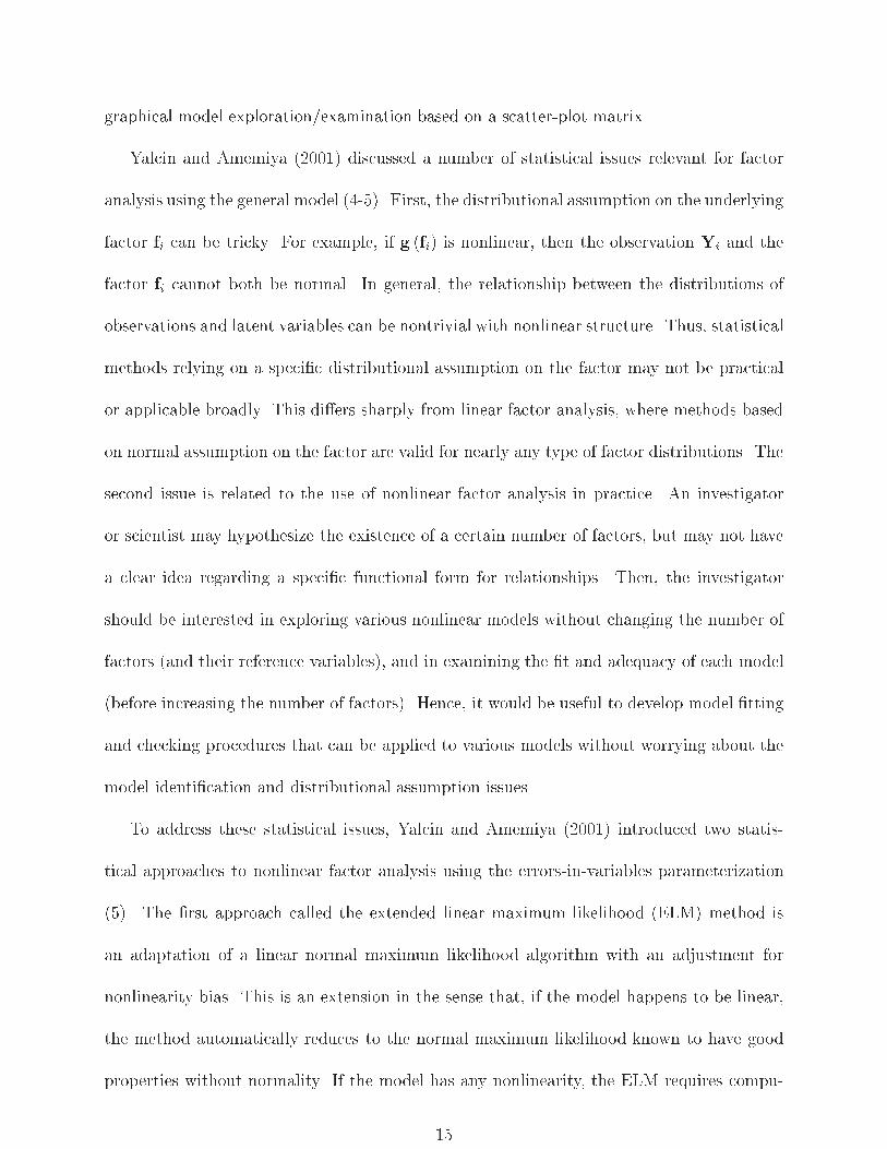
Yalcin and Amemiya (2001) discussed a number of statistical issues relevant for factor

analysis using the general model (4-5). First, the distributional assumption on the underlying

factor fi can be tricky. For example, if g (fi) is nonlinear, then the observation Yi and the

factor fi cannot both be normal. In general, the relationship between the distributions of

observations and latent variables can be nontrivial with nonlinear structure. Thus, statistical

methods relying on a speci�c distributional assumption on the factor may not be practical

or applicable broadly. This di�ers sharply from linear factor analysis, where methods based

on normal assumption on the factor are valid for nearly any type of factor distributions. The

second issue is related to the use of nonlinear factor analysis in practice. An investigator

or scientist may hypothesize the existence of a certain number of factors, but may not have

a clear idea regarding a speci�c functional form for relationships. Then, the investigator

should be interested in exploring various nonlinear models without changing the number of

factors (and their reference variables), and in examining the �t and adequacy of each model

(before increasing the number of factors). Hence, it would be useful to develop model �tting

and checking procedures that can be applied to various models without worrying about the

model identi�cation and distributional assumption issues.

To address these statistical issues, Yalcin and Amemiya (2001) introduced two statis-

tical approaches to nonlinear factor analysis using the errors-in-variables parameterization

(5). The �rst approach called the extended linear maximum likelihood (ELM) method is

an adaptation of a linear normal maximum likelihood algorithm with an adjustment for

nonlinearity bias. This is an extension in the sense that, if the model happens to be linear,

the method automatically reduces to the normal maximum likelihood known to have good

properties without normality. If the model has any nonlinearity, the ELM requires compu-

15

tation of factor score estimates designed for nonlinear models, and evaluation of some terms

at such estimates at each iteration. However, the method was developed to avoid the inci-

dental parameter problem. In this sense, the ELM is basically a �xed-factor approach, and

can be useful without specifying the distributional form for the factor. The computation of

the factor score estimate for each individual at each iteration can lead to possible numerical

instability and �nite sample statistical inaccuracy, as evidenced in the paper's simulation

study. This is a reason why Yalcin and Amemiya (2001) suggested an alternative approach.

Their second approach, the approximate conditional likelihood (ACL) method, uses the

errors-in-variables parameterization (5), and an approximated conditional distribution of Yi

given Xi. The method is also an application of the pseudo likelihood approach, and con-

centrates on obtaining good estimates for the relationship parameter � and error variances

avoiding the use and full estimation of the factor distribution. Accordingly, the ACL method

can be used also for a broad class of factor distributions, although the class is not as broad

as that for the ELM. However, with the simpler computation, the ACL tends to be more

stable numerically than the ELM.

A common feature for the ELM and ACL is that, given a speci�c errors-in-variables

formulation with p and q (dimensions of the observed and factor vectors) satisfying

(p� q)(p� q + 1)

2� p; (6)

almost any nonlinear model g (fi;�) can be �tted and its goodness of �t can be statistically

tested. Note that the condition (6) is the counting-rule identi�cation condition for the un-

restricted (exploratory) linear factor analysis model (a special case of the general nonlinear

model). Thus, given a particular number of factors, both methods can be used to explore dif-

ferent linear and nonlinear models and to perform statistical tests to assess/compare models.

16

For both, the tests are based on error contrasts (de�ned di�erently for the two methods),

and have an asymptotic chi-square distribution with degrees of freedom (p�q)(p�q+1)2

�p under

the model speci�cation.

The overall discussion and approach in Yalcin and Amemiya (2001) are insightful for

formulating nonlinear factor analysis and addressing statistical issues involved in the analysis.

Their proposed model �tting and checking procedures are promising, but can be considered

a good starting point in methodological research for nonlinear factor analysis. The issue

of developing useful statistical methods for nonlinear factor analysis (addressing all aspects

of analyses speci�c to factor analysis but not necessarily always relevant for the structural

equation modeling) with minimal assumption on the factor distribution requires further

investigation.

3 Development of nonlinear structural equation anal-

ysis

With the introduction and development of LISREL (J�oreskog and S�orbom, 1981) in the late

1970's and early 1980's, came a dramatic increase in the use of structural models with latent

or unmeasured variables in the social sciences (Bentler, 1980). There was an increased focus

on modeling and estimating the relationship between variables in which some of the variables

may be measured with error. But, as the name \LISREL" transparently points out, it is a

model and method for dealing with linear relationships thus limited in its ability to exibly

match complicated nonlinear theories.

17

3.1 Measurement error cross-product model

Focusing on a common nonlinear relationship of interest, Busemeyer and Jones (1983)

pointed out in their introduction that \Multiplicative models are ubiquitous in psychological

research". The kind of multiplicative model, Busemeyer and Jones (1983) were referring to

is the following `interaction' or `moderator' model

f3 = �0 + �1f1 + �2f2 + �3f1f2 + � (7)

where the latent variables (constructs) of interest f1, f2, and f3 are possibly all measured

with error. Busemeyer and Jones (1983) showed the serious deleterious e�ects of increased

measurement error on the detection and interpretation of interactions, \multiplying variables

measured with error ampli�es the measurement error problem". They refer to Bohrnstedt

and Marwell (1978) who provided a method for taking this ampli�ed measurement error

into account dependent on prior knowledge of the reliabilities of the measures for f1 and f2

and strong assumptions of their distributions. Feucht (1989) also demonstrates methods for

\correcting" for the measurement error when reliabilities for the measures of latent variables

were known outlining the strengths and drawbacks of the work of Heise (1986) and Fuller

(1980, 1987). Lewbinski and Humphreys (1990) further showed that not only could modera-

tor e�ects (like the f1f2 term in (7)) be missed, but that they could in some circumstances be

incorrectly found when, in fact, there was some other non modeled nonlinear relationship in

the structural model. McClelland and Judd (1993) provide a nice summary of the plentiful

literature lamenting the di�culties of detecting moderator e�ects giving earliest reference

to Zedeck (1971). They go on to point out that one of the main problems is \�eld stud-

ies, relative to experiments, have non-optimal distributions of f1 and f2 and this means the

e�ciency of the moderator parameter estimate and statistical power is much lower." (p.386)

18

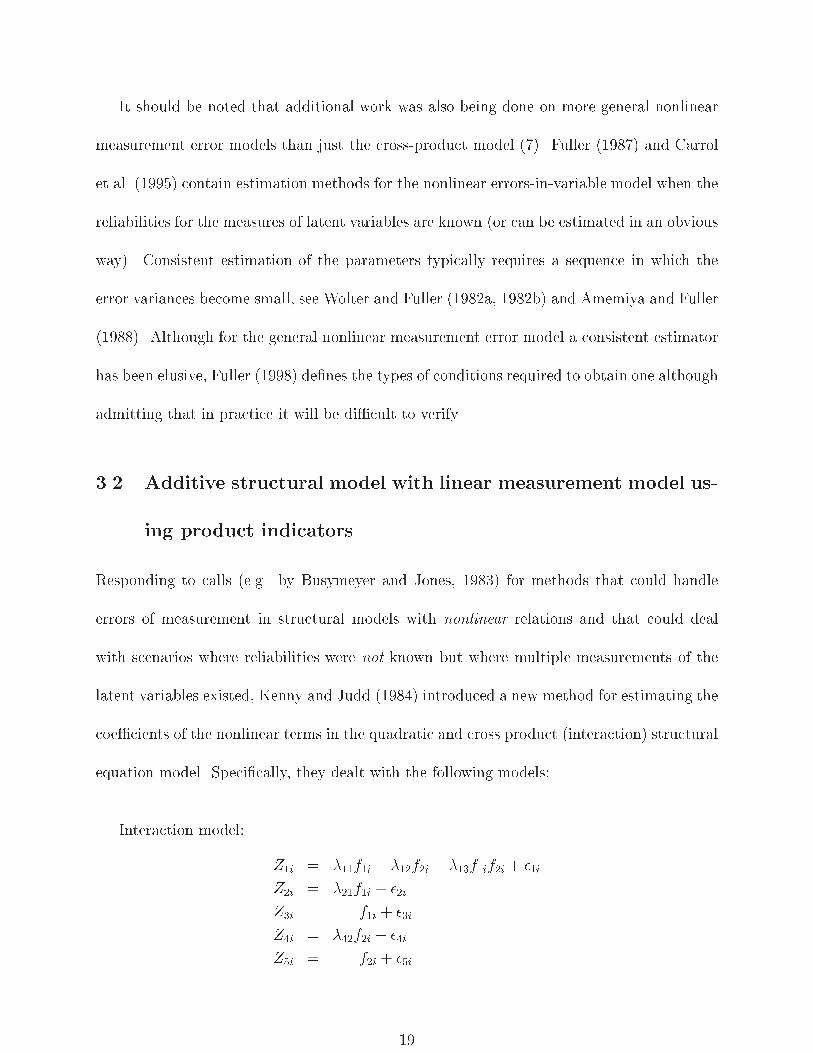
It should be noted that additional work was also being done on more general nonlinear

measurement error models than just the cross-product model (7). Fuller (1987) and Carrol

et al. (1995) contain estimation methods for the nonlinear errors-in-variable model when the

reliabilities for the measures of latent variables are known (or can be estimated in an obvious

way). Consistent estimation of the parameters typically requires a sequence in which the

error variances become small, see Wolter and Fuller (1982a, 1982b) and Amemiya and Fuller

(1988). Although for the general nonlinear measurement error model a consistent estimator

has been elusive, Fuller (1998) de�nes the types of conditions required to obtain one although

admitting that in practice it will be di�cult to verify.

3.2 Additive structural model with linear measurement model us-

ing product indicators

Responding to calls (e.g. by Busymeyer and Jones, 1983) for methods that could handle

errors of measurement in structural models with nonlinear relations and that could deal

with scenarios where reliabilities were not known but where multiple measurements of the

latent variables existed, Kenny and Judd (1984) introduced a new method for estimating the

coe�cients of the nonlinear terms in the quadratic and cross product (interaction) structural

equation model. Speci�cally, they dealt with the following models:

Interaction model:

Z1i = �11f1i + �12f2i + �13f1if2i + �1i

Z2i = �21f1i + �2i

Z3i = f1i + �3i

Z4i = �42f2i + �4i

Z5i = f2i + �5i

19

Quadratic model:

Z1i = �11f1i + �12f21i + �1i

Z2i = �21f1i + �2i

Z3i = f1i + �3i

Note that these models are, in fact, just special cases of Zi = �+�g(fi) + �i with some

elements of � �xed to 1 or 0. Nevertheless, no reference was given in Kenny and Judd

(1984) to any previous nonlinear factor analysis work. The basic idea of Kenny and Judd

(1984) was to create new \observed variables" by taking products of existing variables and

use these as additional indicators of the nonlinear terms in the model. For example, for the

interaction model, consider

0BBBBBBBBBBBB@

Z1i

Z2i

Z3i

Z4i

Z5i

Z2iZ4i

Z2iZ5i

Z3iZ4i

Z3iZ5i

1CCCCCCCCCCCCA

=

0BBBBBBBBBBBB@

�11�211000000

�1200�4210000

�130000

�21�42�21�421

1CCCCCCCCCCCCA

0@

f1if2i

f1if2i

1A+

0BBBBBBBBBBBB@

�1i�2i�3i�4i�5iu1iu2iu3iu4i

1CCCCCCCCCCCCA

;

where

u1i = �21f1i�4i + �42f2i�2i + �2i�4i

u2i = �21f1i�5i + f2i�2i + �2i�5i

u3i = f1i�4i + �42f2i�3i + �3i�4i

u4i = f1i�5i + f2i�3i + �3i�5i :

Assuming fi and �i are normally distributed, Kenny and Judd (1984) construct the co-

variance matrix of (f1i; f2i; f1if2i)0 and (�0;u0)0. This results in many (tedious) constraints on

the model covariance matrix. Despite the cumbersome modeling restrictions, this product

indicator method of Kenny and Judd (1984) was possible to implement in existing linear

structural equation modeling software programs (e.g. LISREL).

20

The Kenny and Judd (1984) technique attracted methodological discussions and alter-

ations by a number of papers, including Hayduk (1987), Ping (1995, 1996a, 1996b,1996c),

Jaccard and Wan (1995, 1996), Joreskog and Yang (1996, 1997), Li et al. (1998) as well

as several similar papers within Schumacker and Marcoulides (1998). But, the method has

been shown to produce inconsistent estimators when the observed indicators are not nor-

mally distributed (Wall and Amemiya, 2001). The generalized appended product indicator

or GAPI procedure of Wall and Amemiya (2001) used the general idea of Kenny and Judd

(1984) of creating new indicators, but stopped short of assuming normality for the underlying

factors and instead allowed the higher order moments to be estimated directly rather than

be considered functions of the �rst and second moments (as in the case when normality is

assumed). The method produces consistent estimators without assuming any distributional

form for the underlying factors or errors. Indeed this robustness to distributional assump-

tions is an advantage, yet still the GAPI procedure, like the Kenny Judd procedure entails

the rather ad-hoc step of creating new product indicators and sorting through potentially

tedious restrictions. Referring to Kenny and Judd (1984), MacCallum and Mar (1995) write

\Their approach is somewhat cumbersome in that one must construct multiple indica-tors to represent the nonlinear e�ects and one must determine nonlinear constraints tobe imposed on parameters of the model. Nevertheless, this approach appears to be themost workable method currently available. An alternative method allowing for directestimation of multiplicative or quadratic e�ects of latent variables without constructingadditional indicators would be extremely useful. (p.418)"

3.3 Additive structural model with linear measurement model

The model motivating Busemeyer and Jones (1983), Kenny and Judd (1984) and those

related works involved the product of two latent variables or the square of a latent variable in

a single equation. Those papers proved to be the spark for a urry of methodological papers

introducing a new modeling framework and new estimation methods for the \nonlinear

21

structural equation model".

Partitioning fi into endogenous and exogenous variables, i.e. fi = (�i; �i)0, the nonlinear

structural equation model is

Zi = �+�fi + �i (8)

�i = B�i + �g(�i) + �i :

Assuming the exogenous factors �i and errors �i and �i are normally distributed, a

maximum likelihood method should theoretically be possible. The nature of latent variables

as \missing data" lends one to consider the use of the EM algorithm (Dempster, Laird and

Rubin, 1977) for maximum likelihood estimation for (8). But because of the necessarily

nonnormal distribution of �i arising from any nonlinear function in g(�i), a closed form

for the observed data likelihood is not possible in general. Klein, et al. (1997) and Klein

and Moosbrugger (2000) proposed a mixture distribution to approximate the nonnormal

distribution arising speci�cally for the interaction model and used this to adapt the EM

algorithm to produce maximum likelihood estimators. Then Lee and Zhu (2002) develop the

ML estimation for the general model (8) using recent statistical and computational advances

in the EM algorithms available for computing ML estimates for complicated models. In

particular, owing to the complexity of the model, the E-step is intractable and is solved by

using the Metropolis-Hastings algorithm. Furthermore the M-step does not have a closed

form and thus conditional maximization is used (Meng and Rubin, 1993). Finally, bridge

sampling is used to determine convergence of the MCECM algorithm (Meng and Wong,

1996). This same computational framework for producing ML estimates is then naturally

used by Lee et al. (2003) in the case of ignorably missing data. The method is then further

extended to the case where the observed variables Zi may be both continuous or polytomous

22

(Lee and Song, 2003a) assuming the underlying variable structure with thresholds relating

the polytomous items to the continuous factors. Additionally a method for model diagnostics

has been also proposed for the nonlinear SEM using maximum likelihood (Lee and Lu 2003)

At the same time that computational advances to the EM algorithm were being used

for producing maximum likelihood estimates for the parameters in model (8), very similar

simulation based computational algorithms for fully Bayesian inference were being applied

to the same model. Given distributions for the underlying factors and errors and priors

(usually non-informative priors) for the unknown parameters, Markov Chain Monte Carlo

(MCMC) methods including the Gibbs sampler and Metropolis-Hastings algorithm can be

relatively straightforwardly applied to (8). Wittenberg and Arminger (1997) worked out

the Gibbs sampler for the special case cross-product model while Arminger and Muth�en

(1998) described the Bayesian method generally for (8). Zhu and Lee (1999) also present

basically the same method as Arminger and Muth�en but provide a Bayesian goodness-of-

�t assessment. Lee and Zhu (2000) describe the fully Bayesian estimation for the model

extended to include both continuous and polytomous observed variables Zi (like Lee and

Song (2003a) do for maximum likelihood estimation) and Lee and Song (2003b) provide a

method for model comparison within the Bayesian framework. Finally, the Bayesian method

has further been shown to work for an extended model that allow for multigroup analysis

(Song and Lee, 2002).

While the Maximum likelihood and Bayesian methods provide appropriate inference when

the distributional assumptions of the underlying factors and errors are correct, they may pro-

vide severely biased results when these non-checkable assumptions are incorrect. Moreover,

there is a computational burden attached to both the ML and Bayesian methods for the

nonlinear structural equation model due to the fact that some simulation based numerical

23

method is required.

Bollen (1995, 1996) developed a two-stage least squares method for �tting (8) which

gives consistent estimation without specifying the distribution for f and additionally has a

closed form. The method uses the instrumental variable technique where instruments are

formed by taking functions of the observed indicators. One di�culty of the method comes

from �nding an appropriate instrument. Bollen (1995) and Bollen and Paxton (1998) show

that the method works for the quadratic and interaction model but for general g(�i) it may

be impossible to �nd appropriate instruments. For example, Bollen (1995) points out that

the method may not work for the cubic model without an adequate number of observed

indicators.

Wall and Amemiya (2000, 2003) introduced a two-stage method of moments (2SMM)

procedure for �tting (8) when the nonlinear g(�i) part consists of general polynomial terms.

Like Bollen's method, the 2SMM produces consistent estimators for the structural model

parameters for virtually any distribution of the observed indicator variables. The procedure

uses factor score estimates in a form of nonlinear errors-in-variables regression and produces

closed-form method of moments type estimators as well as asymptotically correct standard

errors. Simulation studies in Wall and Amemiya (2000, 2003) have shown that the 2SMM

outperforms in terms of bias e�ciency and coverage probability Bollen's two stage least

squares method. Intuition for this comes from the fact that the factor score estimates used

in 2SMM are shown to be the pseudo-su�cient statistics for the structural model parameters

in (8) and as such are fully using the information in the measurement model to estimate the

structural model.

24

3.4 General nonlinear structural equation analysis

Two common features in the nonlinear structural equation models considered in Subsections

3.1-3.3 are the use of a linear measurement model and the restriction to additive structural

models. (The linear simultaneous coe�cient form in (8) gives only parametric nonlinear

restrictions, and the reduced form is still additive in latent variables.) Also, many of the

reviewed methods focus on estimation of a single structural equation, and may not be readily

applicable in addressing some factor analytic issues. From the point of view that the factor

analysis model is a special case of the structural equation model with no structural model,

the methods reviewed in the previous subsections may not be considered to be nonlinear

factor analysis methods. From another point of view, the structural equation system is a

special case of the factor analysis model, when the structural model expressed in a reduced

form is substituted into the measurement model, or when each endogenous latent variable

has only one observed indicator in the separate measurement model and the equation and

measurement errors are confounded. According to this, the nonlinear structural equation

methods covered in 3.1-3.3 are applicable only for particular special cases of the general non-

linear factor analysis model in Subsection 2.4. In this subsection, following the formulation

in Subsection 2.4 and related work by Amemiya and Zhao (2001, 2002), we present a general

nonlinear structural equation system that is su�ciently general to cover or to be covered by

the general nonlinear factor analysis model in 2.4.

For a continuous observed vector Zi and a continuous factor vector fi, the general nonlin-

ear factor analysis model (4) or its form in the errors-in-variables parameterization (5) is a

natural measurement model. A structural model can be interpreted as a set of relationships

among the elements of fi with equation errors. Then, a general structural model can be

25

expressed as

H(fi;�0) = �i; (9)

where ei is a zero-mean r � 1 equation error, and an r-valued function H(�;�0) speci�es

relationships. This matches with the practice of expressing simultaneous equations from the

subject-matter concern, each with a zero-mean deviation term. This model (9) is not given

in an identi�able form, because fi can be transformed in any nonlinear way or the implicit

function H(�) can be altered by, e.g., the multiplication of an r � r matrix. One way to

eliminate this factor/function indeterminacy is to consider an explicit reduced form. Solving

(9) for r components of fi in terms of other q � r components, an explicit reduced form

structural model is

�i = h(�i;�); (10)

where

fi =

0BB@

�i

�i

1CCA ;

�i =

0BB@

�i

�i

1CCA ; (11)

and � is the original equation error in (9). In general, solving a nonlinear implicit function (9)

results in the equation error term � entering the explicit function h nonlinearly. Considering

only models given in this explicit reduced form, the general nonlinear structural model

does not have the factor/function indeterminacy with an identi�able parameter �. Some

structural models, e.g., a recursive model, can be written in an unambiguous way without

solving in an explicit reduced form. But, the explicit reduced form (10) provides a uni�ed

framework for the general nonlinear structural model.

26

By substituting the reduced form structural model (10) into the general nonlinear factor

measurement model (5), we obtain an observation reduced form of the general nonlinear

structural equation system

Zi =

0BBBBBB@

g (h(�i;�); �i;�)

h(�i;�)

�i

1CCCCCCA

+ �i : (12)

This can be considered the general structural equation model in the measurement errors-in-

variables parameterization and the structural reduced form. Written in this way, the general

nonlinear structural equation system (12) is a nonlinear factor analysis model with a factor

vector �i in (11). This model is similar to the errors-in-variables general nonlinear factor

analysis model (5), except that �i, a part of the factor vector, does not have a reference

observed variable but is restricted to have mean zero. The work of Amemiya and Zhao

(2001, 2002) is being extended to develop statistical methods appropriate for the general

nonlinear structural equation model (12).

4 Conclusion

In the last 100 years, the development of statistical methods for factor analysis has been mo-

tivated by scienti�c and practical needs, and has been driven by advancement in computing.

This is also true for nonlinear factor analysis. As reviewed here, the needs for considering

nonlinearity from scienti�c reasons were pointed out very early. But, the methodological

research has become active only in recent years with the wide availability of the computing

capabilities. Also, as in the linear case, the introduction of the LISREL or structural equa-

tion modeling was in uential. The errors-in-variables (reference-variable) parameterization

27

and the relationship-modeling approach, both made popular by LISREL, have been helpful

in developing model formulation approaches and model �tting methods.

Nonlinear methodological research has broadened the scope and the applicability of factor

analysis as a whole. The interdependency among multivariate observations are no longer

assessed only through correlations and covariances, but can now be represented by complex

relationship models. Important subject-matter questions involving nonlinearity, such as the

existence of a cross-product or interaction e�ect, can now be addressed using nonlinear factor

analysis methods.

As discussed in Subsections 2.4 and 3.4, the general formulation of nonlinear factor and

structural equation analyses has emerged recently. This is an important topic for understand-

ing the theoretical foundation and uni�cation of such analyses. In this general context, there

are a number of issues that can bene�t from further development of statistical methods. One

such issue is the basic factor analysis concern of determining the number of underlying factors

or the dimensionality of nonlinear underlying structure. In general, more complete and useful

methods for exploring multivariate data structure, rather than for �tting a particular model,

are welcome. Another issue lacking proper methodology is the instrument assessment and de-

velopment incorporating possibly nonlinear measurements. Also, the development of useful

statistical procedures that are applicable without assuming a speci�c factor distributional

form will continue to be a challenge in nonlinear factor analysis methodology. Nonlinear

multi-population and longitudinal data analyses need to be investigated as well. Nonlinear

factor analysis methodological development is expected to be an active area of research for

years to come.

28

5 References

Amemiya, Y. (1993a). On nonlinear factor analysis. Proceedings of the Social Statistics

Section, the Annual Meeting of the American Statistical Association, 290{294. Asso-

ciation, 92{96.

Amemiya, Y. (1993b). Instrumental variable estimation for nonlinear factor analysis. Mul-

tivariate Analysis: Future Directions 2, C. M. Cuadras and C. R. Rao, eds., Elsevier,

Amsterdam, 113{129.

Amemiya, Y. and Fuller, W.A. (1988). Estimation for the nonlinear function relationship

Annals of Statistics, 16, 147-160.

Amemiya, Y. and Zhao, Y. (2001). Estimation for nonlinear structural equation system with

an unspeci�ed distribution. Proceedings of Business and Economic Statistics Section,

the Annual Meeting of the American Statistical Association (CD-ROM).

Amemiya, Y. and Zhao, Y. (2002). Pseudo likelihood approach for nonliear and non-

normal structural equation analysis. Business and Economic Statistics Section, the

Annual Meeting of the American Statistical Association (CD-ROM).

Arminger, G and Muth�en, B. (1998). A Bayesian approach to nonlinear latent variable

models using the Gibbs sampler and the Metropolis-Hastings algorithm. Psychome-

trika, 63(3), 271-300.

Bartlett, M.S. (1953). Factor analysis in psychology as a statistician sees it, in Uppsala

Symposium on Psychological Factor Analysis, Nordisk Psykologi's Monograph Series

No. 3, 23-34. Copenhagen: Ejnar Mundsgaards; Stockholm: Almqvist and Wiksell.

29

Bentler, P.M. (1980). Multivariate analysis with latent variables: Causal modeling Annual

Review of Psychology, 31, 419-457.

Bohrnstedt, G.W. and Marwell, G. (1978). The reliability of products of two random

variables In KF Schuessler (Ed.), Sociological Methodology San Francisco: Jossey-Bass.

Bollen, K.A. (1995). Structural equation models that are nonlinear in latent variables: A

least squares estimator. Sociological Methodology, 223-251.

Bollen, K.A. (1996). An alternative two stage least squares (2SLS) estimator for latent

variable equation. Psychometrika,.

Bollen, K.A. and Paxton, P. (1998). Interactions of latent variables in structural equation

models Structural equation modeling, 267-293.

Browne, M.W. (1984). Asymptotically distribution free methods for the analysis of co-

variance structures, British Journal of Mathematical and Statistical Psychology, 37,

62-83.

Busemeyer, J.R. and Jones, L.E. (1983). Analysis of multiplicative combination rules when

the causal variables are measured with error. Psychological Bulletin, 93, 549-562.

Carroll, R.J., Ruppert D., and Stefanski, L.A. (1995). Measurement error in nonlinear

models, Chapman and Hall, London.

Dempster, A.P., Laird, N.M., Rubin, D.B. (1977). Maximum likelihood from incomplete

data via the EM algorithm (with discussion) Journal of the Royal Statistical Society,

Series B, 39, 1-38.

30

Etezadi-Amoli, J., and McDonald, R.P. (1983). A second generation nonlinear factor anal-

ysis. Psychometrika, 48(3) 315-342.

Ferguson, G.A. (1941). The factorial interpretation of test di�culty Psychometrika, 6(5),

323-329.

Feucht, T. (1989). Estimating multiplicative regression terms in the presence of measure-

ment error. Sociological Methods and Research, 17(3), 257-282.

Fuller, W.A. (1980). Properties of some estimators for the errors-in-variables model Annals

of Statistics, 8, 407-422.

Fuller, W.A. (1987). Measurement error models. New York: John Wiley.

Fuller, W. A. (1998). Estimation for the nonlinear errors-in-variables model. In Galata,

R. and Kchenho�, H. (Eds.) Econometrics in Theory and Practice, Physica-Verlag,

15-21.

Gibson, W.A. (1951). Applications of the mathematics of multiple -factor analysis to prob-

lems of latent structure analysis. Unpublished doctoral dissertation, Univ. Chicago,

1951.

Gibson, W.A. (1955). Nonlinear factor analysis, single factor case. American Psychologist,

10, 438. (Abstract).

Gibson, W.A. (1956). Nonlinear factors in two dimensions. American Psychologist, 11, 415.

(Abstract).

Gibson, W.A. (1959). Three multivariate models: factor analysis, latent structure analysis,

and latent pro�le analysis. Psychometrika, 24, 229-252.

31

Gibson, W.A. (1960). Nonlinear factors in two dimensions. Psychometrika 25, 4, 381-392.

Hastie, T. and Stuetzle, W. (1989). Principal curves. Journal of the American Statistical

Association 84(406), 502-516.

Hayduck, L.A. (1987). Structural equation modeling with LISREL: Essentials and advances.

Heise, D.R. (1986). Estimating nonlinear models correcting for measurement error. Socio-

logical Methods and Research, 14, 447-472.

Honkela, A. (2004). Bayesian algorithms for latent variable models.

Location: http://www.cis.hut.�/projects/bayes/

Jaccard, J., and Wan, C.K. (1995). Measurement error in the analysis of interaction ef-

fects between continuous predictors using multiple regression: Multiple indicator and

structural equation approaches. Psychological Bulletin, 117(2), 348-357.

Jaccard, J., and Wan, C.K. (1996). LISREL approaches to interaction e�ects in multiple

regression, Sage.

J�oreskog, K.G. and S�orbom D (1981). LISREL: Analysis of linear structural relationships

by the method of maximum likelihood. Chicago, IL: National Educational Resources.

J�oreskog, K.G., and Yang, F. (1996). Non-linear structural equation models: The Kenny-

Judd model with interaction e�ects. In G.A. Marcoulides and R.E. Schumacker (Eds.)

Advanced Structural Equation Modeling: Issues and Techniques, 57-88.

J�oreskog, K.G., and Yang, F. (1997). Estimation of interaction models using the augmented

moment matrix: Comparison of asymptotic standard errors. In W. Bandilla and F.

Faulbaum (Eds.) SoftStat '97 Advances in Statistical Software 6, 467-478.

32

Jutten, C. and Karhunen, J. (2004). Advances in Blind Source Separation (BSS) and

Independent Component Analysis (ICA) for Nonlinear Mixtures. To appear in Inter-

national Journal of Neural Systems 14(5).

Kenny, D.A. and Judd, C.M. (1984). Estimating the nonlinear and interactive e�ects of

latent variables. Psychological Bulletin, 96(1), 201-210.

Klein, A., Moosbrugger, H., Schermelleh-Engel, K., Frank, D. (1997). A new approach

to the estimation of latent interaction e�ects in structural equation models. In W.

Bandilla and F. Faulbaum (Eds.) SoftStat '97 Advances in Statistical Software 6,

479-486.

Klein, A., Moosbrugger, H. (2000). Maximum likelihood estimation of latent interaction

e�ects with the LMS method. Psychometrika, 65(4), 457-474.

Lawley, D.N. and Maxwell, A.E. (1963). Factor analysis as a statistical method, London,

Butterworths.

Lazarsfeld, P.F. (1950). The logical and mathematical foundation of laten structure anal-

ysis. In S.A. Stou�er er al., Measurement and prediction Princeton: Princeton Univ.

Press, Ch. 10.

Lee, S.Y. and Zhu, H.T. (2000). Statistical analysis of nonlinear structural equation models

with continuous and polytomous data. British Journal of Mathematical and Statistical

Psychology, 53, 209-232.

Lee, S.Y. and Zhu, H.T. (2002). Maximum likelihood estimation of nonlinear structural

equation models Psychometrika, 67(2), 189-210.

33

Lee, S.Y. and Lu, B. (2003). Case-deletion diagnostics for nonlinear structural equation

models. Multivariate Behavioral Research, 38(3), 375-400.

Lee, S.Y. and Song, X.Y. (2003a). Maximum likelihood estimation and model comparison

of nonlinear structural equation models with continuous and polytomous variables

Computational Statistics and Data Aanalysis, 44, 125-142.

Lee, S.Y. and Song, X.Y. (2003b). Model comparison of nonlinear structural equation

models with �xed covariates. Psychometrika, 68(1), 27-47.

Lee, S.Y., Song, X.Y., and Lee, J.C.K. (2003). Maximum likelihood estimation of nonlinear

structural equation models with ignorable missing data Journal of Educational and

Behavioral Statistics, 28(2), 111-134.

Lewin-Koh, S. C. and Amemiya, Y. (2003). Heteroscedastic factor analysis. Biometrika,

Vol. 90, No. 1, 85{97.

Li, F., Harmer, P., Duncan, T., Duncan, S., Acock, A., and Boles, S. (1998). Approaches

to testing interaction e�ects using structural equation modeling methodology. Multi-

variate Behavioral Research, 33(1), 1-39.

Lubinski, D. and Humphreys, L.G. (1990). Assessing spurious 'moderator e�ects' Illus-

trated substantively with the hypothesized 'synergistic' relation between spatial and

mathematical ability Psychological Bulletin, 107, 385-393.

MacCallum, R.C. and Mar, C.M. (1995). Distinguishing between moderator and quadratic

e�ects in multiple regression. Psychological Bulletin, 118(3), 405-421.

McClelland, G.H. and Judd, C.M. (1993). Statistical Di�culties of detecting interactions

and moderator e�ects, Psychological Bulletin 114(2), 376-390

34

McDonald, R.P. (1962). A general approach to nonlinear factor analysis. Psychometrika,

27(4), 397-415.

McDonald, R.P. (1965). Di�culty factors and nonlinear factor analysis, Psychometrika, 18,

11-23.

McDonald, R.P. (1967a). Numerical methods for polynomial models in nonlinear factor

analysis. Psychometrika, 32(1), 77-112.

McDonald, R.P. (1967b). Factor interaction in nonlinear factor analysis. British Journal

of Mathematical and Statistical Psychology, 20, 205-215.

McDonald, R.P. (1979). The simultaneous estimation of factor loadings and scores. British

Journal of Mathematical and Statistical Psychology, 32, 212-228.

Meng, X.L. and Rubin, D.B. (1993). Maximum likelihood estimation via the ECM al-

goirthm: A general framework. Biometrika, 80, 267-278.

Meng, X.L. and Wong, W.H. (1996). Simulating ratios of normalizing constants via a

simple identity: A theoretical exploration Statistic Sinica, 6, 831-860.

Molenaar, P.C. and Boomsma, D.I. (1986). Application of nonlinear factor analysis to

genotype-environment interactions. Behavior Gentics, 17(1), 71-80.

Mooijaart, A. and Bentler, P. (1986). Random polynomial factor analysis. In Data Analysis

and Informatics, IV (E. Diday et al., Eds.), 241-250.

Ping, R.A. (1995). A parsimonious estimating technique for interaction and quadratic

latent variables. Journal of Marketing Research, 32, 336-347.

35

Ping, R.A. (1996a). Latent variable interaction and quadratic e�ect estimation: A two-step

technique using structural equation analysis. Psychological Bulletin, 119, 166-175.

Ping, R.A. (1996b). Latent variable regression: A technique for estimating interaction and

quadratic coe�cients. Multivariate Behavioral Research, 31, 95-120.

Ping, R.A. (1996c). Estimating latent variable interactions and quadratics: The state of

this art. Journal of Management, 22, 163-183.

Schumacker, R. and Marcoulides, G. (Eds.) (1998). Interaction and nonlinear e�ects in

structural equation modeling. Mahwah, NJ: Lawrence Erlbaum Associates.

Song, X.Y. and Lee, S.Y. (2002). A Bayesian approach for multigroup nonlinear factor

analysis Structural Equation Modeling, 9(4), 523-553.

Taleb, A. (2002). A generic framework for blind source separation in structured nonlinear

models. IEEE Trans on Signal Processing, 50(8): 1819-1830.

Wall, M.M. and Amemiya, Y., (2000). Estimation for polynomial structural equation

models. Journal of the American Statistical Association, 95, 929-940.

Wall, M.M. and Amemiya, Y., (2001). Generalized appended product indicator proce-

dure for nonlinear structural equation analysis. Journal of Educational and Behavioral

Statistics , 26(1), 1-29.

Wall, M.M. and Amemiya, Y., (2003). A method of moments technique for �tting in-

teraction e�ects in structural equation models. British Journal of Mathematical and

Statistical Psychology, 56, 47-63.

36

Wittenberg, J., and Arminger, G. (1997). Bayesian non-linear latent variable models-

speci�cation and estimation with the program system BALAM. In W. Bandilla and F.

Faulbaum (Eds.) SoftStat '97 Advances in Statistical Software 6, 487-494.

Wolter, K.M. and Fuller, W.A. (1982a). Estimation of the quadratic errors-in-variables

model, Biometrika, 69, 175-182.

Wolter, K.M. and Fuller, W.A. (1982b). Estimation of nonlinear errors-in-variables models,

Annals of Statistics, 10, 539-548.

Yalcin, I. and Amemiya, Y. (1993). Fitting of a general nonlinear factor analysis model.

Proceedings of the Statistical Computing Section, the Annual Meeting of the American

Statistical Association, 92{96.

Yalcin, Y. and Amemiya, Y. (1995). An algorithm for additive nonlinear factor analysis.

Proceedings of the Business and Economic Statistics Section, the Annual Meeting of

the American Statistical Association, 326{330.

Yalcin, I. and Amemiya, Y. (2001). Nonlinear factor analysis as a statistical method.

Statistical Science, 16(3), 275-294.

Zedeck, S. (1971). Problems with the use of 'moderator' variables. Psychological Bulletin,

76, 295-310.

Zhu, H.T., Lee, S.Y. (1999). Statistical analysis of nonlinear factor analysis models. British

Journal of Mathematical and Statistical Psychology, 52, 225-242.

37