Applying to SSHRC – How to Support an Application and Tips for Administrators

REVEALED PRICE PREFERENCE: THEORY AND STOCHASTIC TESTING
By
Rahul Deb, Yuichi Kitamura, John K.-H. Quah, and Jörg Stoye
May 2017
COWLES FOUNDATION DISCUSSION PAPER NO. 2087
COWLES FOUNDATION FOR RESEARCH IN ECONOMICS YALE UNIVERSITY
Box 208281 New Haven, Connecticut 06520-8281
http://cowles.yale.edu/

REVEALED PRICE PREFERENCE: THEORY AND STOCHASTIC TESTING
RAHUL DEB, YUICHI KITAMURA, JOHN K.-H. QUAH, AND JORG STOYEG
MAY 16, 2017
ABSTRACT. We develop a model of demand where consumers trade-off the utility of consumptionagainst the disutility of expenditure. This model is appropriate whenever a consumer’s demandover a strict subset of all available goods is being analyzed. Data sets consistent with this modelare characterized by the absence of revealed preference cycles over prices. The model is readilygeneralized to the random utility setting, for which we develop nonparametric statistical tests. Ourapplication on national household consumption data provides support for the model.
1. INTRODUCTION
Imagine a consumer who is asked what quantity she will purchase of L goods at given prices; informal terms, she is asked to choose a bundle xt ∈ RL
+ at the price vector pt ∈ RL++. To fix ideas,
we could think of these goods as grocery items and xt as the monthly purchase of groceries if pt
are the prevailing prices. With T such observations, the data set collected is D = (pt, xt)Tt=1.
What patterns of choices in D should we expect to observe?
There are at least two ways to approach this question. If, at observations t and t′, we find thatpt′ · xt < pt′ · xt′ , then
the consumer has revealed that she strictly prefers the bundle xt′ to the bundle xt.
If this were not true, then either xt or a nearby bundle would be strictly preferred to xt′ and costless, which means the choice of xt′ is not optimal. The standard revealed preference theory ofconsumer demand is built on requiring that this preference over grocery bundles, as revealed by adata set such as D, is internally consistent. In particular, Afriat (1967)’s Theorem says that so longas the consumer’s revealed preferences over bundles do not contain cycles (a property known asthe generalized axiom of revealed preference or GARP, for short) then there is a strictly increasing utilityfunction U : RL
+ → R such that xs maximizes U(x) in the budget set x ∈ RL+ : ps · x ≤ ps · xs,
GUNIVERSITY OF TORONTO, YALE UNIVERSITY, JOHNS HOPKINS UNIVERSITY AND BONN UNIVERSITY.E-mail addresses: [email protected], [email protected], [email protected],
[email protected] are very grateful for the comments provided by the seminar participants at the Cowles Foundation Conferences(April 2015, June 2015), University of Toronto (March 2016), Heterogeneity in Supply and Demand Conference at BostonCollege (December 2016), Identification of Rationality in Markets and Games Conference at Warwick University (March2017), University of Cambridge (March 2017), UCSD (April 2017), UCLA (April 2017) and the Canadian EconomicTheory Conference (May 2017). Deb thanks the SSHRC for their generous financial support. Stoye acknowledgessupport from NSF grant SES-1260980 and through Cornell University’s Economics Computer Cluster Organization,which was partially funded through NSF Grant SES-0922005. We thank Matthew Thirkettle for excellent researchassistance.
1

2 DEB, KITAMURA, QUAH, AND STOYE
for every observation s = 1, 2, ..., T.1 Notice that this theory implicitly assumes that it makes senseto speak of the consumer’s preference over groceries, independently of her consumption of othergoods, currently or in the future. In formal terms, this requires that the consumer has a preferenceover grocery bundles that is weakly separable from her consumption of all other goods.2
But, presented with the same data set D = (pt, xt)Tt=1, it would be entirely natural for us (as
observers) to think along different lines; instead of inferring the consumer’s preference over gro-cery bundles from the observations, we could draw conclusions about the consumer’s preferenceover prices. If at observations t and t′, we find that pt′ · xt < pt · xt, then
the consumer has revealed that she strictly prefers the price pt′ to the price pt.
This is because, at the price vector pt′ the consumer can, if she wishes, buy the bundle bought atthe price pt and would still have money left for the purchase of other, non-grocery, consumptiongoods. (Put another way, if pt and pt′ are the prices at two grocery stores and the consumer couldchoose to go to one store or the other, then the observations in D will lead us to conclude thatshe will opt for the store where the prices are pt′ .) This concept of revealed preference recognizesthat there are alternative uses to money besides groceries and that expenditure on groceries has anopportunity cost. Is it possible to build a revealed preference theory of consumer demand basedon this alternate requirement that the consumer’s preference over grocery prices, as revealed bythe data set D, is internally consistent; if so, what would such a theory look like? The objectiveof this paper is to answer this question and to demonstrate the appealing features of a theory ofrevealed price preference.
1.1. The expenditure-augmented utility model
We show that the absence of revealed preference cycles over prices — a property we call the gen-eralized axiom of revealed price preference or GAPP, for short — has a very natural characterization. Itis both necessary and sufficient for the existence of a strictly increasing function U : RL
+×R− → R
such that xs ∈ arg maxx∈RL+
U(x,−ps · x) for all s = 1, 2, ..., T. The function U should be interpretedas an expenditure-augmented utility function, where U(x,−e) is the consumer’s utility when she ac-quires x at the cost of e. Unlike the standard consumer optimization problem, notice that the con-sumer does not have a budget constraint; instead, she is deterred from choosing arbitrarily largebundles by the increasing expenditure it incurs, which reduces her utility. This is a reduced formutility function which implicitly holds fixed all other variables that may be relevant to the con-sumer’s preference over (x,−e); these variables could include the consumer’s wealth, the pricesof other goods which the consumer considers relevant to her consumption decision on these Lgoods, etc.
1The term GARP is from Varian (1982), which also contains a proof of the result. An extension of Afriat’s Theorem tononlinear budget sets can also be found in Forges and Minelli (2009).2The consumer’s overall utility function will have the form V(U(x), z), where U is the utility function defined overgrocery bundles x, z is the bundle of all other goods consumed by the consumer and V is the overall utility function.
REVEALED PRICE PREFERENCE 3
Besides being behaviorally compelling in its own right, the expenditure-augmented utility modelhas two distinctive features that makes it a worthwhile alternative to the standard model. (i) No-tice that the marginal rate of substitution between two goods at a given bundle x ∈ RL
+ will typ-ically depend on the expenditure incurred in acquiring that bundle; it follows that the marginalrate of substitution can vary with unobserved goods (whose consumption levels could changeas e changes). In other words, our model does not require the assumption of weak separabilityand so it could be appropriate is situations where that assumption is problematic. (ii) Essentiallybecause the standard model only tries to model the agent’s preference among bundles of the Lgoods, the only price information it requires are the prices of those goods relative to each other: itdoes not require the researcher to have any information on the prices of any other good that theconsumer may also purchase. This modest informational requirement is an important advantagebut it also means that the model cannot tell us anything about the consumer’s overall welfare whenthe prices for the L goods change. On the other hand our model recognizes that expenditure levelsare endogenous (i.e., chosen by the consumer at the observed prices) and exploits this to comparethe consumer’s welfare at different prices for the L goods; in fact, as we have pointed out, themodel is characterized by this feature.
In the theoretical literature in public economics and industrial organization, it is common toassume individuals have quasilinear utility functions. In addition to tractability, this assump-tion ensures that the difference in consumer surplus due to price changes is an exact measure ofthe change in welfare (as it coincides with the compensating and equivalent variations) becausequasilinearity ensures that there are no income effects.3 This is a special case of our model, withU(x, e) = H(x)− e for some real-valued and increasing function H. Our approach allows greaterflexibility in the form of the utility function U and, in particular, does not require a constant mar-ginal disutility of expenditure, which imposes strong and sometimes implausible restrictions ondemand.
In the empirical literature, welfare changes are often calculated by explicitly introducing a nu-meraire good over and above the L goods being examined and then imputing demand for thisnumeraire good by using data on (for example) annual income; one could then calculate the im-pact on welfare following prices changes on these L goods at a given income and a given price forthe numeraire good.4 Obviously, compared with this approach, ours is useful when informationon income is not available (which is a feature of many commonly used data sets). But even whenthis information is available, by not using it, we are avoiding taking a stand on the precise budgetfrom which the consumer draws her expenditure on these L goods; for example, the consumercould mentally set aside some expenditure for a group of commodities containing these L goodsand this ‘mental budget’ may differ from the annual income (see Thaler (1999)). That said, ourapproach does rely on the assumption that consumer’s utility function U is stable over the period
3See, for instance, Varian (1985), Schwartz (1990) and the papers that follow.4For recent work using this approach, see Blundell, Horowitz, and Parey (2012) and Hausman and Newey (2016). Inboth these papers, the empirical application involves the case where L = 1 (specifically, the good examined is gasoline,so it is a two-good demand system when the numeraire is included); when L = 1, our approach imposes no meaningfulrestrictions on data so it does not readily provide a viable alternative way to study the specific empirical issues in thosepapers.

4 DEB, KITAMURA, QUAH, AND STOYE
where her demand is observed; presumably large changes to the consumer’s wealth (both hercurrent resources and her future prospects) will have an impact on U, so in effect we are assumingthat these fluctuations are modest.
1.2. Testing the expenditure-augmented utility model
After formulating the expenditure-augmented utility model and exploring its theoretical fea-tures, the second part of our paper is devoted to testing it empirically. We could in principle testthis model on panel data sets of household or individual demand, for example, from informationon purchasing behavior collected from scanner data. Tests and applications of the standard modelusing Afriat’s Theorem or its extensions are very common,5 and our model could be tested onthis data in the same fashion; GAPP is just as straightforward to test as GARP on a panel dataset.6 Rather than doing this, we develop a random utility version of our model and implement aneconometric test of this version instead. There are at least three reasons why it is useful to developsuch a model. (i) The random utility model is more general in that it allows for individual prefer-ences in the population to change over time, provided the population distribution of preferencesstays the same; this weaker assumption may be appropriate for data sets that span longer timehorizons. (ii) The random utility version can be applied to repeated cross sectional data and doesnot require panel data sets. (iii) Perhaps most importantly, nonparametric statistical procedurescould be naturally introduced to test the random utility model and so we can go beyond the binarypass-fail tests of the nonstochastic expenditure augmented-utility model.
McFadden and Richter (1991) have formulated a random utility version of the standard modelthat could be used to test data collected from repeated cross sections. They assume that the econo-metrician observes the distribution of demand choices on each of a finite number of budget setsand characterize the observable content of this model, under the assumption that the distributionof preferences is stable across observations. Their key observation is that, notwithstanding thepotentially infinite number of possible preference types generating the observed demand distri-butions, it is possible to partition this infinite set to a finite number of equivalence classes withthe members of each class generating demand conforming to a particular pattern.7 This in turnguarantees that the observations are rationalizable by a random version of the standard model ifand only if there is a solution to a linear program constructed from the data.
Unfortunately, the process of actually applying the test devised by McFadden and Richter is infact rather complicated, simply because observational data does not typically come in the formthey have assumed. Indeed a population of consumers will have different expenditure levels atthe same prices and, what is worse, these expenditure levels are chosen by the consumers them-selves, so one simply does not directly observe the distribution of demand when all consumersare subjected to the same budget set. Recently, Kitamura and Stoye (2013) have implemented atest based on the McFadden-Richter model but they could only do so by first estimating, at each
5For a recent survey, see Crawford and De Rock (2014).6It is also common to test the standard model in experimental settings. Note that, our test is not appropriate on typicalexperimental data where the budget is provided exogenously (and is not endogenous as in our model) as part of theexperiment.7The number of classes is bounded above by a formula that depends on the number of distinct budget sets.

REVEALED PRICE PREFERENCE 5
observed price vector, the distribution of demand at a common expenditure level (distinct fromthose expenditure levels actually observed). Nonparametric estimation of this type is not impos-sible, but it does require the use of instrumental variables with all its attendant assumptions.
We devise a test of the random utility version of our model and show that it is both easier toimplement and requires no additional data (such as an instrumental variable) in contrast to thetest of the McFadden-Richter model. We assume that the econometrician observes the distributionof demand at a finite set of price vectors. At each price vector, expenditure levels need not becommon across consumers but can vary across consumers and across different price vectors, sothis corresponds almost exactly to the characteristics of observational data on demand. We showthat such a data set can be generated by a stable distribution of expenditure-augmented utilityfunctions if and only if there is a solution to a family of linear inequalities constructed from thedata. When a solution exists, its solution gives the proportion of consumers belonging to each of afinite number of utility classes. Through these solutions, we also obtain upper and lower boundson the proportion of consumers who are revealed better off, or worse off, at one price vectorcompared to another. In short, not only can we test the stochastic version of the expenditure-augmented utility model, the test also furnishes useful information on the welfare impact of pricechanges on the population of consumers.
1.3. Organization of the paper
The remainder of this paper is structured as follows. Section 2 lays our the deterministic modeland its revealed preference characterization, and Section 3 generalizes it to our analog of a Ran-dom Utility Model. Section 4 lays out the novel econometric theory needed to test this, Section 5illustrates with an empirical application, and Section 6 concludes.
2. THE DETERMINISTIC MODEL
The primitive in the analysis in this section is a data set of a single consumer’s purchasingbehavior collected by an econometrician. The econometrician observes the consumer’s purchasingbehavior over L goods and the prices at which those goods were chosen. In formal terms, thebundle is in RL
+ and the prices are in RL++ and so an observation t can be represented as (pt, xt) ∈
RL++ ×RL
+. The data set collected by the econometrician is D := (pt, xt)Tt=1. We will slightly
abuse notation and use T both to refer to the number of observations, which we assume is finite,and the set 1, . . . , T; the meaning will be clear from the context. Similarly, L could denote boththe number, and the set, of commodities.
We shall begin with a short description of Afriat’s Theorem. This provides the background toour model (especially for readers unfamiliar with that result) and, additionally, we employ it toprove some of our results.

6 DEB, KITAMURA, QUAH, AND STOYE
2.1. Afriat’s Theorem
Given a data set D := (pt, xt)Tt=1, a locally nonsatiated8 utility function U : RL
+ → R is saidto rationalize D if
xt ∈ argmaxx∈RL
+ : ptx≤ptxtU(x) for all t ∈ T. (1)
This is the standard notion of rationalization and the one addressed by Afriat’s Theorem. It re-quires that there exists a utility function such that each observed bundle xt maximizes utility inthe budget set given by the observed prices pt and expenditure ptxt.
A basic concept used in Afriat’s Theorem is that of revealed preference. This is captured by twobinary relations, x and x, defined on the chosen bundles observed in D, that is, the set X :=xtt∈T. These revealed preference relations are defined as follows:
xt′ x (x)xt if xt′ pt′ ≥ (>)xt pt′ .
We say that the bundle xt′ is directly revealed preferred to xt if xt′ x xt, that is, whenever the bundlext is cheaper at prices pt′ than the bundle xt. If xt is strictly cheaper, so xt′ x xt, we say that xt′ isdirectly revealed strictly preferred to xt. This terminology is, of course, very intuitive. If the agent ismaximizing some locally nonsatiated utility function U, then if xt′ x xt (xt′ x xt), it must implythat U(xt′) ≥ (>)U(xt).
We denote the transitive closure of x by ∗x, that is, for xt′ and xt in X , we have xt′ ∗x xt ifthere are t1, t2,...,tN in T such that xt′ x xt1 , xt1 x xt2 , . . . , xtN−1 x xtN , and xtN x xt′ ; in thiscase, we say that xt′ is revealed preferred to xt. If anywhere along this sequence, it is possible toreplace x with x then we say that xt′ is revealed strictly preferred to xt and denote that relation byxt′ ∗x xt. Once again, this terminology is completely natural since if D is rationalizable by somelocally nonsatiated utility function U, then xt′ ∗x (∗x)xt implies that U(xt′) ≥ (>)U(xt).
Definition 2.1. A data set D = (pt, xt)Tt=1 satisfies the Generalized Axiom of Revealed Prefer-
ence or GARP if there do not exist two observations t, t′ ∈ T such that xt′ ∗x xt and xt ∗x xt′ .
Afriat showed that this condition is necessary and sufficient for rationalization.
Afriat’s Theorem (Afriat (1967)). Given a data set D = (pt, xt)Tt=1, the following are equivalent:
(1) D can be rationalized by a locally nonsatiated utility function(2) D satisfies GARP.(3) D can be rationalized by a strictly increasing, continuous, and concave utility function.
REMARK 1. The proof that the rationalizability of D implies GARP is straightforward to show (itessentially follows from the discussion preceding the statement of the theorem), so the heart of thetheorem lies in showing that GARP implies that D can be rationalized. The standard proof (forinstance, see Fostel, Scarf, and Todd (2004)) works by showing that a consequence of GARP is thatthere exist numbers φt and λt > 0 (for all t ∈ T) that solve the inequalities
φt′ ≤ φt + λt pt · (xt′ − xt) for all t′ 6= t. (2)
8This means that at any bundle x and open neighborhood of x, there is a bundle y in the neighborhood with strictlyhigher utility.
REVEALED PRICE PREFERENCE 7
It is then straightforward to show that
U(x) = mint∈T
φt + λt pt · (x− xt)
(3)
rationalizes D, with the utility of the observed consumption bundles satisfying U(xt) = φt. Thefunction U is the lower envelope of a finite number of strictly increasing affine functions, and so itis strictly increasing, continuous, and concave. A remarkable feature of this theorem is that whileGARP follows simply from local nonsatiation of the utility function, it is sufficient to guaranteethat D is rationalized by a utility function with significantly stronger properties.
REMARK 2. To be precise, GARP guarantees that there is preference% (in other words, a complete,reflexive, and transitive binary relation) on X that extends the (potentially incomplete) revealedpreference relations ∗x and ∗x in the following sense: if xt′ ∗x xt, then xt′ % xt and if xt′ ∗xxt then xt′ xt. One could then proceed to show (and this is less obvious) that, for any suchpreference%, the inequalities (2) admit a solution with the property that φt′ ≥ (>)φt if xt′ % ()xt
(see Quah (2014)). Hence, for any preference % that extends the revealed preference relations,there is in turn a utility function U that rationalizes D and extends % (from X to RL
+) in thesense that U(xt′) ≥ (>)U(xt) if xt′ % ()xt. This has implications on the inferences one coulddraw from the data. If xt′ 6%∗x xt then it is always possible to find a preference extending therevealed preference relations such that xt xt′ . Similarly, if xt′ ∗x xt but xt′ 6∗x xt then onecould find a preference extending the revealed preference relations such that xt′ ∼ xt.9 Therefore,xt′ ∗x (∗x)xt if and only if every locally nonsatiated utility function rationalizing D has theproperty that U(xt′) ≥ (>)U(xt).
REMARK 3. A feature of Afriat’s Theorem that is less often remarked upon is that in fact U, asgiven by (3), is well-defined, strictly increasing, continuous, and concave on the domain RL, ratherthan just the positive orthant RL
+. Furthermore,
xt ∈ argmaxx∈RL : ptx≤ptxt
U(x) for all t ∈ T. (4)
In other words, xt is optimal even if U is extended beyond the positive orthant and x can be chosenfrom the larger domain. (Compare (4) with (1).) This curiosity will turn out to be rather convenientwhen we apply Afriat’s Theorem in our proofs.
2.2. Consistent welfare comparisons across prices
Typically, the L goods whose demand is being monitored by the econometrician constitutes nomore than a part of the purchasing decisions made by the consumer. The consumer’s true budget(especially when one takes into account the possibility of borrowing and saving) is never observedand the expenditure which she devotes to the L goods is a decision made by the consumer anddependent on prices (of the L goods and possibly on the prices of other goods as well). The con-sumer’s choice over the L goods inevitably affects what she could afford on, and therefore herconsumption of, other goods not observed by the econometrician; given this, the rationalizationcriterion (1) used in Afriat’s Theorem will only make sense under an additional assumption of
9We use xt′ ∼ xt to mean that xt′ % xt and xt % xt′ .

8 DEB, KITAMURA, QUAH, AND STOYE
weak separability: the consumer has a sub-utility function U defined over the L goods and theutility function of the consumer, defined over all goods, takes the form H(U(x), y), where x isthe bundle of L goods observed by the econometrician and y is the bundle of unobserved goods.Assuming that the consumer chooses (x, y) to maximize G(x, y) = H(U(x), y), subject to a bud-get constraint px + qy ≤ M (where M is her wealth and p and q are the prices of the observedand unobserved goods respectively), then, at the prices pt, the consumer’s choice xt will obey (1)provided H is strictly increasing in either the first or second argument. This provides the theo-retical motivation to test for the existence of a sub-utility function U that rationalizes a data setD = (pt, xt)T
t=1. Notice that once the weak separability assumption is in place, the backgroundrequirements of Afriat’s test are very modest in the sense that it is possible for prices of the unob-served goods and the unobserved total wealth to change arbitrarily across observations, withoutaffecting the validity of the test. This is a major advantage in applications but the downside is thatthe conclusions of this model are correspondingly limited to ranking different bundles among theobserved goods via the sub-utility function.
Now suppose that instead of checking for rationalizability in the sense of (1), the econometricianwould like to ask a different question: given a data set D = (pt, xt)T
t=1, can he sign the welfareimpact of a price change from pt to pt′? Stated differently, this question asks whether he cancompare the consumer’s overall utility after a change in the prices of the L goods from pt and pt′ ,holding fixed other aspects of the economic environment that may affect the consumer’s welfare,such as the prices of unobserved goods and her overall wealth. Perhaps the most basic welfarecomparison in this setting can be made as follows: if at prices pt′ , the econometrician finds thatpt′xt < ptxt then he can conclude that the agent is better off at the price vector pt′ compared to pt.This is because, at the price pt′ the consumer can, if she wishes, buy the bundle bought at pt andshe would still have money left over to buy other things, so she must be strictly better off at pt′ .This ranking is eminently sensible, but can it lead to inconsistencies?
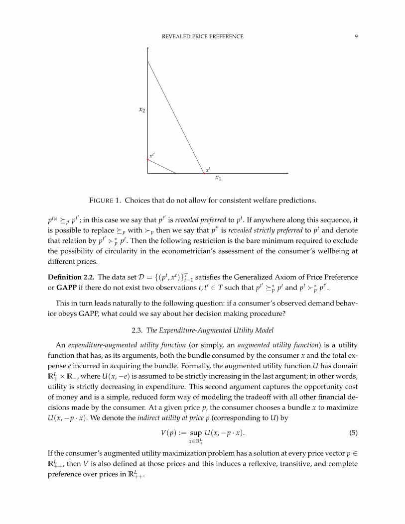
Example 1. Consider a two observation data set
pt = (2, 1) , xt = (4, 0) and pt′ = (1, 2) , xt′ = (0, 1).
which is depicted in Figure 1. Given that the budget sets do not even cross, we know that GARPholds. Since pt′xt < ptxt, it seems that we may conclude that the consumer is better off at pricespt′ than at pt; however, it is also true that pt′xt′ > ptxt′ , which gives the opposite conclusion.
This example shows that for an econometrician to be able to consistently compare the con-sumer’s welfare at different prices, some restriction (different from GARP) has to be imposed onthe data set. To be precise, define the binary relations p and p on P := ptt∈T, that is, the setof price vectors observed in D, in the following manner:
pt′ p (p)pt if pt′xt ≤ (<)ptxt.
We say that price pt′ is directly revealed preferred to pt if pt′ p pt, that is, whenever the bundle xt ischeaper at prices pt′ than at prices pt. If it is strictly cheaper, so pt′ p pt, we say that pt′ is directlyrevealed strictly preferred to pt. We denote the transitive closure ofp by∗p, that is, for pt′ and pt inP , we have pt′ ∗p pt if there are t1, t2,...,tN in T such that pt′ p pt1 , pt1 p pt2 ,..., ptN−1 p ptN , and
REVEALED PRICE PREFERENCE 9
This for a data set
pt = (2, 1) , xt = (4, 0) and pt′ = (1, 2) , xt′ = (0, 1).
that violates GAPP.
x1
x2
bxt
bxt′
3
FIGURE 1. Choices that do not allow for consistent welfare predictions.
ptN p pt′ ; in this case we say that pt′ is revealed preferred to pt. If anywhere along this sequence, itis possible to replace p with p then we say that pt′ is revealed strictly preferred to pt and denotethat relation by pt′ ∗p pt. Then the following restriction is the bare minimum required to excludethe possibility of circularity in the econometrician’s assessment of the consumer’s wellbeing atdifferent prices.
Definition 2.2. The data set D = (pt, xt)Tt=1 satisfies the Generalized Axiom of Price Preference
or GAPP if there do not exist two observations t, t′ ∈ T such that pt′ ∗p pt and pt ∗p pt′ .
This in turn leads naturally to the following question: if a consumer’s observed demand behav-ior obeys GAPP, what could we say about her decision making procedure?
2.3. The Expenditure-Augmented Utility Model
An expenditure-augmented utility function (or simply, an augmented utility function) is a utilityfunction that has, as its arguments, both the bundle consumed by the consumer x and the total ex-pense e incurred in acquiring the bundle. Formally, the augmented utility function U has domainRL
+×R−, where U(x,−e) is assumed to be strictly increasing in the last argument; in other words,utility is strictly decreasing in expenditure. This second argument captures the opportunity costof money and is a simple, reduced form way of modeling the tradeoff with all other financial de-cisions made by the consumer. At a given price p, the consumer chooses a bundle x to maximizeU(x,−p · x). We denote the indirect utility at price p (corresponding to U) by
V(p) := supx∈RL
+
U(x,−p · x). (5)
If the consumer’s augmented utility maximization problem has a solution at every price vector p ∈RL
++, then V is also defined at those prices and this induces a reflexive, transitive, and completepreference over prices in RL
++.

10 DEB, KITAMURA, QUAH, AND STOYE
A data set D = (pt, xt)Tt=1 is rationalized by an augmented utility function if there exists such a
function U : RL+ ×R− → R with
xt ∈ argmaxx∈RL
+
U(x,−pt · x) for all t ∈ T.
Notice that unlike the notion of rationalization in Afriat’s Theorem, we do not require the bundlex to be chosen from the budget set x ∈ RL
+ : ptx ≤ ptxt. The consumer can instead choose fromthe entire consumption space RL
+, though expenditure is taken into account since more costlybundles will depress the consumer’s utility.
It is straightforward to see that GAPP is necessary for a data set to be rationalizable by anaugmented utility function. Suppose GAPP were not satisfied but the data could be rationalizednonetheless by some augmented utility function U. Then, for some t, t′, t1, . . . , tN ∈ T, its indirectutility V would satisfy
V(pt′) ≥ V(pt1) ≥ · · · ≥ V(ptN ) ≥ V(pt) > V(pt′)
which is impossible.Our main theoretical result, which we state next, also establishes the sufficiency of GAPP for
rationalization. Moreover, the result states that whenever D can be rationalized, it can be ratio-nalized by an augmented utility function U with a list of properties that make it convenient foranalysis. In particular, we can guarantee that there is always a solution to maxx∈RL
+U(x,−p · x)
for any p ∈ RL++. This property guarantees that U will generate preferences over all the price
vectors in RL++. Clearly, it is also necessary for making out-of-sample predictions and, indeed, it
is important for the internal consistency of the model.10
Theorem 1. Given a data set D = (pt, xt)Tt=1, the following are equivalent:
(1) D can be rationalized by an augmented utility function.(2) D satisfies GAPP.(3) D can be rationalized by an augmented utility function U that is strictly increasing, continuous,
and concave. Moreover, U is such that maxx∈RL+
U(x,−p · x) has a solution for all p ∈ RL++.
Proof. We will show that (2) =⇒ (3). We have already argued that (1) =⇒ (2) and (3) =⇒ (1)by definition.
Choose a number M > maxt ptxt and define the augmented data set D = (pt, 1), (xt, M −ptxt)T
t=1. This data set augments D since we have introduced an L + 1th good, which we havepriced at 1 across all observations, with the demand for this good equal to M− ptxt.
The crucial observation to make here is that
(pt, 1)(xt, M− ptxt) ≥ (pt, 1)(xt′ , M− pt′xt′) if and only if pt′xt′ ≥ ptxt′ ,
which means that
(xt, M− ptxt) x (xt′ , M− pt′xt′) if and only if pt p pt′ .
10Suppose the data set is rationalized but only by an augmented utility function for which the existence of an optimumis not generally guaranteed, then it undermines the hypothesis tested since it is not clear why the sample collectedshould then have the property that an optimum exists.
REVEALED PRICE PREFERENCE 11
Similarly,
(pt, 1)(xt, M− ptxt) > (pt, 1)(xt′ , M− pt′xt′) if and only if pt′xt′ > ptxt′ ,
and so(xt, M− ptxt) x (xt′ , M− pt′xt′) if and only if pt p pt′ .
Consequently,D satisfies GAPP if and only if D satisfies GARP. Applying Afriat’s Theorem, whenD satisfies GARP, there is U : RL+1 → R such that
(xt, M− ptxt) ∈ argmaxx∈RL
+ :ptx+m≤MU(x, m) for all t ∈ T.
The function U can be chosen to be strictly increasing, continuous, and concave, and the lower en-velope of a finite set of affine functions. Note that augmented utility function U : RL
+ ×R− → R
defined by U(x,−e) := U(x, M− e) rationalizesD as xt solves maxx∈RL+
U(x,−pt · x) by construc-tion. Furthermore, U is strictly increasing in (x,−e), continuous, and concave.
It remains to be shown that U can be maximized at all p ∈ RL++. Let h : R+ → R be a differen-
tiable function with h(0) = 0, h′(r) > 0 and h′′(r) > 0. Note that these properties guarantee thatlimr→∞ h(r) = ∞. Define U : RL
+ ×R− → R by
U(x,−e) := U(x,−e)− h(max0, e−M). (6)
It is clear that this function is strictly increasing in (x,−e), continuous, and concave. Further-more, xt solves maxx∈RL
+U(x,−pt · x). This is because U(x,−e) ≤ U(x,−e) for all (x,−e), and
U(xt,−ptxt) = U(xt,−ptxt). Lastly, we claim that at every p ∈ RL++, argmaxx∈RL
+U(x,−p · x) is
nonempty. Given that U is continuous, this will fail to hold at some price vector p only if thereis a sequence xn ∈ RL
+ such that p · xn → ∞, with U(xn+1,−pxn+1) > U(xn,−pxn). But this isimpossible because the piecewise linearity of U(x,−e) in x and the strict convexity of h impliesthat U(xn,−pxn)→ −∞.
From this point onwards, when we refer to ‘rationalization’ without additional qualifiers, weshall mean rationalization with an expenditure-augmented utility function, i.e., in the sense estab-lished by Theorem 1 rather than in the sense established by Afriat’s Theorem. It is clear that theinclusion of expenditure in the augmented utility function captures the opportunity cost incurredby the consumer when she chooses some bundle of L goods. Theorem 1 says that this is preciselythe form the utility function should take if we require the data set to obey GAPP, but note thatthe theorem does not require us to subscribe to a specific — or indeed, any — ‘more fundamental’model from which the augmented utility function could be derived. We could, for example, in-terpret the augmented utility function as a representation of a preference over bundles of L goodsand their associated expenditure that the consumer has developed as a habit and which guidesher purchasing decisions.
That said, the proof of Theorem 1 itself provides a particular interpretation for the augmentedutility function. We could suppose that the consumer is maximizing an overall utility functionthat depends both on the observed bundle x and on other goods y, subject to an overall wealth ofM, that is, the consumer is maximizing the overall utility G(x, y) subject to px + qy ≤ M, where
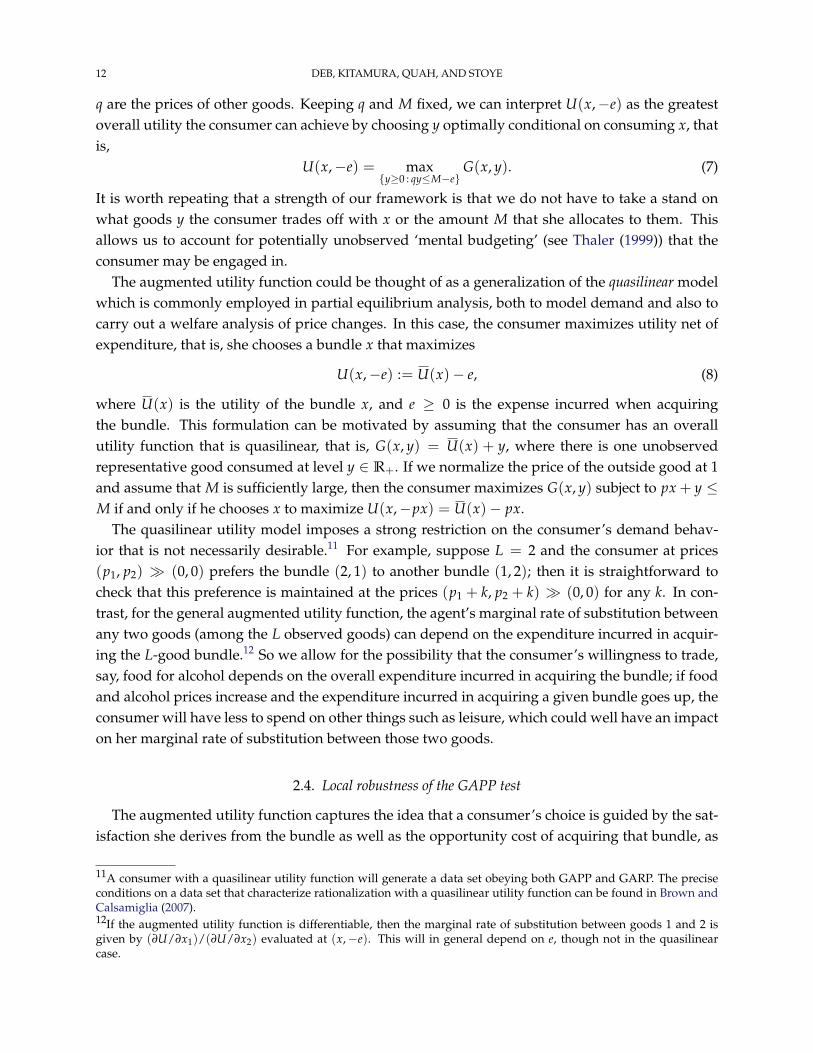
12 DEB, KITAMURA, QUAH, AND STOYE
q are the prices of other goods. Keeping q and M fixed, we can interpret U(x,−e) as the greatestoverall utility the consumer can achieve by choosing y optimally conditional on consuming x, thatis,
U(x,−e) = maxy≥0 : qy≤M−e
G(x, y). (7)
It is worth repeating that a strength of our framework is that we do not have to take a stand onwhat goods y the consumer trades off with x or the amount M that she allocates to them. Thisallows us to account for potentially unobserved ‘mental budgeting’ (see Thaler (1999)) that theconsumer may be engaged in.
The augmented utility function could be thought of as a generalization of the quasilinear modelwhich is commonly employed in partial equilibrium analysis, both to model demand and also tocarry out a welfare analysis of price changes. In this case, the consumer maximizes utility net ofexpenditure, that is, she chooses a bundle x that maximizes
U(x,−e) := U(x)− e, (8)
where U(x) is the utility of the bundle x, and e ≥ 0 is the expense incurred when acquiringthe bundle. This formulation can be motivated by assuming that the consumer has an overallutility function that is quasilinear, that is, G(x, y) = U(x) + y, where there is one unobservedrepresentative good consumed at level y ∈ R+. If we normalize the price of the outside good at 1and assume that M is sufficiently large, then the consumer maximizes G(x, y) subject to px + y ≤M if and only if he chooses x to maximize U(x,−px) = U(x)− px.
The quasilinear utility model imposes a strong restriction on the consumer’s demand behav-ior that is not necessarily desirable.11 For example, suppose L = 2 and the consumer at prices(p1, p2) (0, 0) prefers the bundle (2, 1) to another bundle (1, 2); then it is straightforward tocheck that this preference is maintained at the prices (p1 + k, p2 + k) (0, 0) for any k. In con-trast, for the general augmented utility function, the agent’s marginal rate of substitution betweenany two goods (among the L observed goods) can depend on the expenditure incurred in acquir-ing the L-good bundle.12 So we allow for the possibility that the consumer’s willingness to trade,say, food for alcohol depends on the overall expenditure incurred in acquiring the bundle; if foodand alcohol prices increase and the expenditure incurred in acquiring a given bundle goes up, theconsumer will have less to spend on other things such as leisure, which could well have an impacton her marginal rate of substitution between those two goods.
2.4. Local robustness of the GAPP test
The augmented utility function captures the idea that a consumer’s choice is guided by the sat-isfaction she derives from the bundle as well as the opportunity cost of acquiring that bundle, as
11A consumer with a quasilinear utility function will generate a data set obeying both GAPP and GARP. The preciseconditions on a data set that characterize rationalization with a quasilinear utility function can be found in Brown andCalsamiglia (2007).12If the augmented utility function is differentiable, then the marginal rate of substitution between goods 1 and 2 isgiven by (∂U/∂x1)/(∂U/∂x2) evaluated at (x,−e). This will in general depend on e, though not in the quasilinearcase.

REVEALED PRICE PREFERENCE 13
measured by its expense. This opportunity cost depends on the prices of the alternative (unob-served) goods, so in empirical applications of the GAPP test (especially on data that spans longtime horizons), it would make sense to deflate the prices of the observed goods by an appropriateprice index (to account for price changes of the unobserved goods). Given that these indices areimperfect, the deflated prices of the observed goods pt used for testing may well differ from theirtrue values qt, which introduces an observational error into the data set. Put differently, at timet, the consumer actually maximizes U(x,−qtx) instead of U(x,−ptx) which is the hypothesis weare testing.
Another potential source of error is that the agent’s unobserved wealth may change from oneobservation to the next and this could manifest itself as a change in the consumer’s stock of therepresentative outside good. If this happens, then at observation t, the consumer would be max-imizing U(x,−ptx + δt), where δt is the perturbation in wealth at time t, instead of maximizingU(x,−ptx). Of course, the errors could potentially enter simultaneously in both prices and wealth.
Proposition 1 below shows that inference from a GAPP test is unaffected as long as the size ofthe errors are bounded (equation (9) provides the specific bound). Specifically, so long asD obeys amild genericity condition (which is satisfied in our empirical application), the GAPP test is locallyrobust in the sense that any conclusion obtained through the test remains valid for sufficientlysmall perturbations of the original hypothesis. For example, a data set that fails GAPP is notconsistent with the maximization of an augmented utility function, for all prices sufficiently closeto the ones observed and after allowing for small wealth perturbations.
Not surprisingly, if the errors are allowed to be unbounded, then the model ceases to have anycontent. Specifically, we can always find wealth perturbations δt (while prices pt are assumed tobe measured without error) such that each xt maximizes U(x,−ptx + δt), with no restrictions onD. In particular, these perturbations can be chosen to be mean zero.
Proposition 1. Given a data set D = (pt, xt)Tt=1, the following hold:
(1) There exists an augmented utility function U and δtTt=1, with ∑T
t=1 δt = 0, such that xt ∈argmaxx∈RL
+U(pt,−ptxt + δt) for all t ∈ T.
(2) Suppose, D satisfies ptxt − pt′xt 6= 0 for all t 6= t′ and let qtTt=1 and δtT
t=1 satisfy
2 maxt∈T|δt|+ 2B max
t∈T,i∈L|εt
i | < mint,t′∈T,t 6=t′
|ptxt − pt′xt| (9)
where B = maxt∈T∑Li=1 |xt
i | and εti := qt
i − pti .
If D obeys GAPP, there is an augmented utility function U such that
xt ∈ argmaxx∈RL
+
U(qt,−qtxt + δt) for all t ∈ T, (10)
and if D violates GAPP, then there is no augmented utility function U such that (10) holds.
Proof. Our proof of part (1) relies on a result of Varian (1988), which says that given any dataset D, there always exist ztT
t=1 such that the augemented data set ((pt, 1), (xt, zt))Tt=1 obeys
GARP. By Afriat’s Theorem, there is a utility function U : RL+1 → R such that (xt, zt) is optimalin the budget set (x, z) ∈ RL ×R : ptx + z ≤ Mt, where Mt = zt + ptxt. Afriat’s Theoremalso guarantees that this utility function has various nice properties and, in particular, U can be

14 DEB, KITAMURA, QUAH, AND STOYE
chosen to be strictly increasing. Let M = ∑Tt=1 Mt/T and define the augmented utility function
U : RL+ × R− → R by U(x,−e) := U(x, M − e). Then since U is strictly increasing, xt solves
maxx∈RL+
U(x, δt − ptx) where δt = Mt − M.There are two claims in (2). We first consider the case whereD obeys GAPP. Note that whenever
pt′xt′ − ptxt′ < 0, then for any qtTt=1 and δtT
t=1 such that (9) holds, we obtain pt′xt′ − ptxt′ <
δt′ − εt′xt′ − δt + εtxt′ . This inequality can be re-written as
− qtxt′ + δt < −qt′xt′ + δt′ . (11)
Choose a number M > maxt(qtxt− δt) and define the data set D = (qt, 1), (xt, M+ δt− qtxt)Tt=1.
Since (11) holds whenever pt′xt′ − ptxt′ < 0,
(qt, 1)(xt, M + δt − qtxt) > (qt, 1)(xt′ , M + δt′ − qt′xt′) only if pt′xt′ > ptxt′ .
This guarantees that D obeys GARP since D obeys GAPP. By Afriat’s Theorem, there is a strictlyincreasing utility function U : RL → R such that (xt, M + δt − qtxt) is optimal in the budget set(x, z) ∈ RL+1 : qtx + z ≤ M + δt. Define the augmented utility function U : RL
+ ×R− → R byU(x,−e) := U(x, M− e). Since U is strictly increasing, xt solves maxx∈RL
+U(x, δt − qtx).
Now consider the case where D violates GAPP. Observe that whenever pt′xt′ − ptxt′ > 0, thenfor any qtT
t=1 and δtTt=1 such that (9) holds, we obtain pt′xt′ − ptxt′ > δt′ − εt′xt′ − δt + εtxt′ .
This inequality can be re-written as
− qtxt′ + δt > −qt′xt′ + δt′ . (12)
By way of contradiction, suppose there is an augmented utility function U such that xt maximizesU(x,−qtx + δt) for all t. For any observation t, we write Vt := maxx∈RL U(x,−qtx + δt). Since(12) holds, we obtain
Vt ≥ U(xt′ ,−qtxt′ + δt) > U(xt′ ,−qt′xt′ + δt′) = Vt′ .
Thus, we have shown that Vt > Vt′ whenever pt′xt′ − ptxt′ > 0. Since D violates GAPP there isa finite sequence
(pt1 , xt1
), . . . ,
(ptN , xtN
)of distinct elements in D, such that pti xti+1 < pti+1 xti+1
for all i ∈ 1, . . . , N − 1 and ptN xt1 < pt1 xt1 . By the observation we have just made, we obtainVt1 > Vt2 > ...VtN > Vt1 , which is impossible.
2.5. Comparing GAPP and GARP
Recall that Example 1 in Section 2.2 is an example of a data set that obeys GARP but fails GAPP.We now present an example of a data set that obeys GAPP but fails GARP.
Example 2. Consider the data set consisting of the following two choices:
pt = (2, 1) , xt = (2, 1) and pt′ = (1, 4) , xt′ = (0, 2).
These choices are shown in Figure 2. This is a classic GARP violation as pt · xt = 5 > 2 = pt · xt′
(xt x xt′) and pt′ · xt′ = 8 > 6 = pt′ · xt (xt′ x xt). In words, each bundle is strictly cheaper thanthe other at the budget set corresponding to the latter observation. However, these choices satisfyGAPP as pt′ · xt′ = 8 > 2 = pt · xt′ (pt p pt′) but pt · xt = 5 6 = pt′ · xt (pt′ p pt).

REVEALED PRICE PREFERENCE 15
This for a data set
pt = (2, 1) , xt = (2, 1) and pt′ = (1, 4) , xt′ = (0, 2).
that violates GARP.
x1
x2
bxt′
b xt
1
FIGURE 2. Choices that satisfy GAPP but not GARP
The upshot of this example is that there are data sets that admit rationalization with an aug-mented utility function that cannot be rationalized in Afriat’s sense (that is, in the sense given by(1)). If we interpret the augmented utility function in the form G(x, y) (given by (7)), then thismeans that while the agent’s behavior is consistent with the maximization of an overall utilityfunction G, this utility function is not weakly separable in the observed goods x. In particular,this implies that the agent does not have a quasilinear utility function (with G(x, y) = U(x) + y),which is weakly separable in the observed goods and will generate data sets obeying both GAPPand GARP.
While GAPP and GARP are not comparable conditions, there is a way of converting a GAPP testinto a GARP test that will prove to be very convenient for us. Given a data set D = (pt, xt)T
t=1,we define the expenditure-normalized version of D as another data set D :=
(pt, xt)
Tt=1, such that
xt = xt/ptxt. This new data set has the feature that pt xt = 1 for all t ∈ T. Notice that the revealedprice preference relations p, p remain unchanged when consumption bundles are scaled. Putdifferently, a data set obeys GAPP if and only if its normalized version also obeys GAPP. Therefore,from the perspective of testing for rationalization (by an augmented utility function) this changein the data set is immaterial. The next proposition makes a different and less obvious observationabout D.
Proposition 2. Let D = (pt, xt)Tt=1 be a data set and let D = (pt, xt)t∈T, where xt = xt/(ptxt),
be its expenditure-normalized version. Then the revealed preference relations %∗p and ∗p on P = ptTt=1
and the revealed preference relations %∗x and ∗x on X = xtTt=1 are related in the following manner:
(1) pt %∗p pt′ if and only if xt %∗x xt′ .(2) pt ∗p pt′ if and only if xt ∗x xt′ .
As a consequence, D obeys GAPP if and only if D obeys GARP.

16 DEB, KITAMURA, QUAH, AND STOYE
Proof. Notice that
pt xt
ptxt ≥ pt xt′
pt′xt′ ⇐⇒ pt′xt′ ≥ ptxt′ .
The left side of the equivalence says that xt %x xt′ while the right side says that pt %p pt′ . Thisimplies (1) since %∗p and %∗x are the transitive closures of %p and %x respectively. Similarly, itfollows from
pt xt
ptxt > pt xt′
pt′xt′ ⇐⇒ pt′xt′ > ptxt′
that xt x xt′ if and only if pt p pt′ , which leads to (2). The claims (1) and (2) together guaranteethat there is a sequence of observations in D that lead to a GAPP violation if and only if theanalogous sequence in D lead to a GARP violation.
As an illustration of how Proposition 2 ‘works,’ compare the data sets in Figure 1 and Figure2 to the expenditure-normalized data sets in Figure 3a and Figure 3b. It can be clearly observedthat the expenditure-normalized data in Figure 3a contains a GARP violation (which implies itdoes not satisfy GAPP) whereas the data in Figure 3b does not violate GARP (and, hence, satisfiesGAPP).
A consequence of Proposition 2 is that the expenditure-augmented utility model can be testedin two ways: (i) we can test GAPP directly, or, (ii) we can normalize the data by expenditure andthen test GARP. If we are simply interested in testing GAPP on a data set D then both methodsare computationally straightforward and there is not much to choose between them: they bothrequire the construction of their (respective) revealed preference relations and testing involveschecking for acyclicity. However, as we shall see in the next section, the indirect procedure sup-plied by Proposition 2 will prove to be very useful for testing in the random augmented utilityenvironment.
This for a data set
pt = (2, 1) , xt = (4, 0) and pt′ = (1, 2) , xt′ = (0, 1).
after normalizing the x’s by dividing with the income.
x1
x2
bxt
bxt′
4
(a) Example 1
This for a data set
pt = (2, 1) , xt = (2, 1) and pt′ = (1, 4) , xt′ = (0, 2)
after normalizing the x’s by dividing with the income.
x1
x2
bxt′
b xt
2
(b) Example 2
FIGURE 3. Expenditure-Normalized Choices

REVEALED PRICE PREFERENCE 17
2.6. Preference over Prices
We know from Theorem 1 that if D obeys GAPP then it can be rationalized by an augmentedutility function with an indirect utility that is defined at all price vectors in RL
++. It is straightfor-ward to check that any indirect utility function V as defined by (5) has the following two proper-ties:
(a) it is nonincreasing in p, in the sense that if p′ ≥ p (in the product order) then V(p′) ≤ V(p),and
(b) it is quasiconvex in p, in the sense that if V(p) = V(p′), then V(βp + (1− β)p′) ≤ V(p) forany β ∈ [0, 1].
Any rationalizable data set D could potentially be rationalized by many augmented utilityfunctions and each one of them will lead to a different indirect utility function. We denote thisset of indirect utility functions by V(D). We have already observed that if pt ∗p (∗p)pt′ thenV(pt) ≥ (>)V(pt′) for any V ∈ V(D); in other words, the conclusion that the consumer prefersthe prices pt to pt′ is fully nonparametric in the sense that it is independent of the precise augmentedutility function used to rationalize D. The next result says that, without further information onthe agent’s augmented utility function, this is all the information on the agent’s preference overprices in P that we could glean from the data. Thus, in our nonparametric setting, the revealedprice preference relation contains the most detailed information for welfare comparisons.
Proposition 3. Suppose D = (pt, xt)Tt=1 is rationalizable by an augmented utility function. Then for
any pt, pt′ in P :
(1) pt ∗p pt′ if and only if V(pt) ≥ V(pt′) for all V ∈ V(D).(2) pt ∗p pt′ if and only if V(pt) > V(pt′) for all V ∈ V(D).
Proof. (1) We have already shown the ‘only if’ part of this claim, so we need to show the ‘if’ partholds. From the proof of Theorem 1, we know that for a large M, it is the case that pt p pt′ ifand only if (xt, M− ptxt) x (xt′ , M− pt′xt′) and hence pt ∗p pt′ if and only if (xt, M− ptxt) ∗x(xt′ , M − pt′xt′). If pt 6∗p pt′ , then (xt, M − ptxt) 6∗x (xt′ , M − pt′xt′) and hence there is a utilityfunction U : RL+1
+ → R rationalizing the augmented data set D such that U(xt, M − ptxt) <
U(xt′ , M − pt′xt′) (see Remark 2 in Section 2.1). This in turn implies that the augmented utilityfunction U (as defined by (6)), has the property that U(xt,−ptxt) < U(xt′ ,−pt′xt′) or, equivalently,V(pt) < V(pt′).
(2) Given part (1), we need only show that if pt ∗p pt′ but pt 6∗p pt′ , then there is some augmentedutility function U such that U(xt,−ptxt) = U(xt′ ,−pt′xt′). To see that this holds, note that if pt ∗ppt′ but pt 6∗p pt′ , then (xt, M− ptxt) ∗x (xt′ , M− pt′xt′) but (xt, M− ptxt) 6∗x (xt′ , M− pt′xt′). Inthis case there is a utility function U : RL+1
+ → R rationalizing the augmented data set D such thatU(xt, M − ptxt) = U(xt′ , M − pt′xt′). This in turn implies that the augmented utility function U(as defined by (6)) satisfies U(xt,−ptxt) = U(xt′ ,−pt′xt′) and so V(pt) = V(pt′).
18 DEB, KITAMURA, QUAH, AND STOYE
3. THE STOCHASTIC MODEL
In this section, we develop the stochastic version of expenditure-augmented utility model. Fol-lowing the treatment we adopted in the deterministic case, we shall begin with an explanation ofthe standard version of the random utility model, as found in McFadden and Richter (1991) andKitamura and Stoye (2013) (henceforth to be referred to, respectively, as MR and KS).
3.1. Rationalization by Random Utility
Suppose that instead of observing single choices on T budget sets, the econometrician observeschoice probabilities on each budget set. Our preferred interpretation is that each observation corre-sponds to the distribution of choices made by a population of consumers and the data set consistsof a repeated cross section of such choice probabilities. This interpretation is appropriate for ourempirical application but an alternative interpretation is that the econometrician observes datafrom a single individual who makes multiple choices at each budget set.
We denote the budget set corresponding to observation t by Bt := x ∈ RL+ : ptx = 1. In
this model, only relative prices matter, so we can scale prices and normalize income to 1 withoutloss of generality. We use πt to denote the probability measure of choices on budget set Bt atobservation t. Thus, for any subset Xt ⊂ Bt, πt(Xt) denotes the probability that the choices lie inthe subset Xt. Following MR and KS, we assume that the econometrician observes the stochasticdata set D := (Bt, πt)T
t=1, which consists of a finite collection of budget sets along with thecorresponding choice probabilities.
For ease of exposition, we also impose the following assumption on the data:
for all t, t′ ∈ T with Bt 6= Bt′ , the choice probabilities satisfy πt(Bt ∩ Bt′
)= 0. (A1)
In other words, the choice probability measure π has no mass where the budget sets intersect.This is convenient because it simplifies some of the definitions that follow.13
A random utility is denoted by a measure µ over the set of locally nonsatiated utility functionsdefined on RL
+, which we denote by U . The data set D is said to be rationalized by a random utilitymodel if there exists a random utility µ such that for all Xt ⊂ Bt,
πt(Xt) = µ(U (Xt)) for all t ∈ T, where U (Xt) :=
U ∈ U : argmax
x∈BtU(x) ∈ Xt
.
In other words, to rationalize D we need to find a distribution on the family of utility functionsthat generates a demand distribution at each budget set Bt corresponding to what was observed.The crucial fact that this problem can be solved via a finite procedure was noted by MR. We nowexplain the method they proposed.
Let B1,t, . . . , BIt,t denote the collection of subsets (called patches in KS) of the budget Bt whereeach subset has as its boundaries the intersection of Bt with other budget sets and/or the boundaryhyperplanes of the positive orthant. Formally, for all t ∈ T and it 6= i′t, each set in B1,t, . . . , BIt,tis closed and convex and, in addition, the following hold:
13This simplification is not conceptually necessary for the procedure described here or its adaptation to our setting inthe next subsection. See the explanations given in KS, all of which also apply here.

REVEALED PRICE PREFERENCE 19
(i) ∪1≤it≤It Bit,t = Bt,
(ii) int(Bit,t) ∩ Bt′ = φ for all t′ 6= t that satisfy Bt 6= Bt′ ,(iii) Bit,t ∩ Bi′t,t 6= φ implies that Bit,t ∩ Bi′t,t ⊂ Bt′ for some t′ 6= t that satisfies Bt 6= Bt′ ,
where int(·) denotes the interior of a set.We use the vector πt ∈ ∆It belonging to the It dimensional simplex to denote the discretized
choice probabilities over the collection
B1,t, . . . , BIt,t
. Formally, coordinate it of πt is given by
πit,t = πt(
Bit,t)
, for all Bit,t ∈
B1,t, . . . , BIt,t
.
Even though there may be t, it, i′t for which Bit,t ∩ Bi′t,t 6= φ (as these sets may share parts oftheir boundaries), Assumption A1 guarantees that πt is still a probability measure since choiceprobabilities on the boundaries of Bit,t have measure 0. We denote π := (π1, . . . , πT)′.
We call a deterministic data set D = (pt, xt)Tt=1 typical if, for all t, there is it such that xt ∈
int(Bit,t) for all t ∈ T; in other words, xt lies in the interior of some patch at each observation. If atypical deterministic data set D = (pt, xt)T
t=1 satisfies GARP, then for all other xt ∈ int(Bit,t), t ∈T, the data set (pt, xt)T
t=1 also satisfies GARP. This is because the revealed preference relationsx,x are determined only by where a choice lies on the budget set relative to its intersection withanother budget. Thus, as far as testing rationality is concerned, all choices in a given set int(Bit,t)
are interchangeable. Therefore, we may classify all typical deterministic data sets according tothe patch occupied by the bundle xt at each budget set Bt. In formal terms, we associate to eachtypical deterministic data set D that satisfies GARP a vector a =
(a1,1, . . . , aIT ,T) where
ait,t =
1 if xt ∈ Bit,t,0 otherwise.
(13)
Notice that we have now partitioned all typical deterministic data sets obeying GARP (of whichthere are infinitely many) into a finite number of distinct classes or types, based on the vector aassociated with each data set. We use A to denote the matrix whose columns consist of all the avectors corresponding to these GARP-obeying types (where the columns can be arranged in anyorder) and use |A| to denote the number of such columns (which is also the number of types).
The problem of finding a measure µ on the family of utility functons to rationalize D is essen-tially one of disaggregating D into rationalizable deterministic data sets or, given Afriat’s Theo-rem, into deterministic data sets obeying GARP. If we ignore non-typical deterministic data sets(which is justified because of Assumption A1), this is in turn equivalent to finding weights on thefinitely many distinct types represented by the columns of A, so that their aggregation at eachobservation coincides with the discretized choice probabilities. The following result summarizesthese observations.
MR Theorem. Suppose that the stochastic data set D = (Bt, πt)Tt=1 satisfies Assumption A1. Then
D is rationalized by a random utility model if and only if there exists a ν ∈ R|A|+ such that the discretized
choice probabilities π satisfy Aν = π.14
14Since any ν that satisfies Aν = π must also satisfy ∑|A|j=1 νj = 1, we do not need to explicitly impose the latter
condition.

20 DEB, KITAMURA, QUAH, AND STOYE
Before we turn to the stochastic version of the expenditure-augmented utility model, it is worthhighlighting an important shortcoming of the setting envisaged by MR : data sets of the formD = (Bt, πt)T
t=1 are typically unavailable. This is because even consumers that face the sameprices on the L observed goods (as is commonly assumed in applications with repeated cross sec-tional data, for instance, Blundell, Browning, and Crawford (2008)) will typically spend differentamounts on these goods and, therefore, the observed choices of the population will lie on differentbudget sets; furthermore, even if one conditions on that part of the population that chooses thesame expenditure level at some vector of prices, as these prices change, they will go on to choosedifferent expenditure levels. The procedure set out by MR to test the random utility model reliesheavily on the stylized environment they assume and it is not at all clear how it could be mod-ified to test the model when expenditure is allowed to be endogenous. Recently, the procedurethey proposed was implemented by KS but, in order to do this, KS first had to (in effect) createa data set of the MR type: this involves estimating (from the actual data) what the distributionof demand would be if, hypothetically, all consumers were restricted to the same budget set. In-evitably, estimating these distributions will require the use of instrumental variables (to get roundthe endogeneity of expenditure) and involve a variety of assumptions on the smoothness of Engelcurves, the nature of unobserved heterogeneity across individuals, etc.
3.2. Rationalization by Random Augmented Utility
Once again the starting point of our analysis is a stochastic data set D := (pt, πt)Tt=1 which
consists of a finite set of distinct prices along with a corresponding distribution over chosen bun-dles. But there is one important departure from the previous section: we no longer require the sup-port of πt to lie on the budget set Bt; instead the support could be any set in RL
+. In other words,we no longer require all consumers to incur the same expenditure at each price observation; eachconsumer in the population can decide how much she wishes to spend on the L observed goodsand this could differ across consumers and across price observations. As we pointed out at theend of Section 3.2, this is the form that data typically takes.
A random expenditure-augmented utility is denoted by a measure µ over the set of augmentedutility functions which we denote by U .
Definition 3.1. The data set D is said to be rationalized by the random augmented utility modelif there exists a random augmented utility µ such that for all Xt ⊂ RL
+,
πt(Xt) = µ(U (Xt)) for all t ∈ T, where U (Xt) :=
U ∈ U : argmaxx∈RL
+
U(x,−ptx) ∈ Xt
.
In actual empirical applications, observations are typically made over time. Therefore, we areeffectively asking whether or not D is generated by a distribution of augmented utility functionsthat is stable over the period where observations are taken. This assumption is plausible if (i)there is no change in the prices of the unobserved goods or, more realistically, that these changescould be adequately accounted for by the use of a deflator, and (ii) there is sufficient stability inthe way consumers in the population view their long term economic prospects, so that there is no
REVEALED PRICE PREFERENCE 21
change in their habitualized willingness to trade off consumption of a bundle of goods in L withthe expenditure it incurs.
The problem of finding a measure µ to rationalize D is essentially one of disaggregating D intodeterministic data sets rationalizable by augmented utility functions or, given Theorem 1, intodeterministic data sets obeying GAPP. Crucially, Proposition 2 tells us that a deterministic data setobeys GAPP if and only if its expenditure-normalized version obeys GARP. It follows that µ existsif and only if the normalized version of the stochastic data set D obeys the condition identified byMR (as stated in Section 3.2).
To set this out more formally, we first define the normalized choice probability π corresponding toπ by scaling observations from the entire orthant onto the budget plane Bt generated by prices pt
and expenditure 1. Formally,
πt(Xt) = πt(
x :x
ptx∈ Xt
), for all Xt ⊂ Bt and all t ∈ T.
We suppose that Assumption A1 holds on the normalized data set (Bt, πt)Tt=1; abusing the ter-
minology somewhat, we shall say that D obeys Assumption A1.15 We then define the patches onthe budgets set Bt (as in Section 3.2) and denote them by
B1,t, . . . , BIt,t
. With these patches in
place, we derive the normalized and discretized choice probabilities πt =
π1,t, . . . , π It,t
from πt byassigning to each πit,t the normalized choice probability πt(Bit,t) corresponding to Bit,t. Finally,we construct the matrix A, whose columns are defined by (13); the columns represent distinctGARP-obeying types, which by Proposition 2 coincides with the distinct GAPP-obeying types.The rationalizability of D can then be established by checking if there are weights on these typesthat, at each observation, generate the observed normalized choice probabilities. The followingresult summarizes these observations.
Theorem 2. Let D = (pt, πt)Tt=1 be a stochastic data set obeying Assumption A1. Then D is rational-
ized by the random augmented utility model if and only if there exists a ν ∈ R|A|+ such that the normalized
and discretized choice probabilities π satisfy Aν = π.
It is worth emphasizing that this theorem provides us with a very clean procedure for test-ing the random augmented utility model. If we were testing the random utility model, then theMR test requires a data set where expenditures are common across consumers as a starting point;since this is not commonly available it would have to be estimated, which in turn requires an ad-ditional econometric procedure with all its attendant assumptions. By contrast, to test the randomaugmented utility model, all we have to do is apply the MR test to the expenditure-normalizeddata set (Bt, πt)T
t=1, which is obtained (via a simple transformation) from the original data setD = (pt, πt)T
t=1. This allows us to determine the rationalizability of D because we know, purelyas a consequence of the theoretical model itself and without any further assumptions, that onedata set is rationalized by a random augmented utility model if and only if the other one is.
15A sufficient condition for A1 is that π assigns 0 probability to sets with a Lebesgue measure of 0. Also, as before,this is merely for ease of exposition: our test does not depend on this assumption and, importantly, the data in ourempirical application satisfies A1.

22 DEB, KITAMURA, QUAH, AND STOYE
We end this subsection with an example that makes explicit the operationalization of Theorem2 using data where the normalized and discretized choice probabilities are determined by thesample frequency of choices.
Example 3. Suppose the econometrician observes the set of ten choices at two price vectors,pt = (2, 1) and pt′ = (1, 2), given by the black points in Figures 4a and 4b. These figures also
Consider a set of choices when the prices are
pt = (2, 1).
These are for illustration of how stochastic GAPP works.
x1
x2
Bt
b
b
b
b
b
b
b
b
b
b
b
b
bb
b
b
b
b
b
b
5
(a) Period t
Consider a set of choices when the prices are
pt = (1, 2).
These are for illustration of how stochastic GAPP works.
x1
x2
Bt′
b
b
b
b
b
b
b
b
b
b
b
b
b b
b
b
b
b
b
b
6
(b) Period t′
This for a data set
pt = (2, 1) , xt = (3, 0) and pt′ = (1, 2) , xt′ = (0, 3).
This picture represents the shares π observed in a data set.
x1
x2
B1,t
B2,t
π1,t = 35
π2,t = 25
B1,t′
B2,t′
π2,t′ = 12π1,t′ = 1
2
b
b
b
b
b
b
b
bb
bb
b
b
b
b
b
b
b
b
b
12
(c) The Normalized and Discretized Empirical ChoiceProbabilities π
FIGURE 4. Observed and Scaled Choice Data
demonstrate how the choices are scaled (to the red points) on to the normalized budget sets. Fig-ure 4c then shows that the choice probabilities
π =
(35
,25
,12
,12
)′
REVEALED PRICE PREFERENCE 23
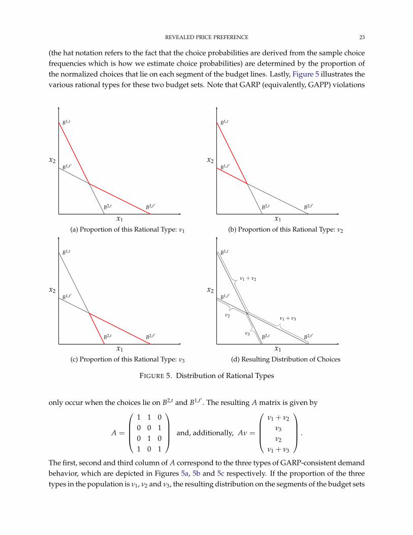
(the hat notation refers to the fact that the choice probabilities are derived from the sample choicefrequencies which is how we estimate choice probabilities) are determined by the proportion ofthe normalized choices that lie on each segment of the budget lines. Lastly, Figure 5 illustrates thevarious rational types for these two budget sets. Note that GARP (equivalently, GAPP) violations
This for a data set
pt = (2, 1) , xt = (3, 0) and pt′ = (1, 2) , xt′ = (0, 3).
We highlight the sets where choices can be made without violating GARP.
x1
x2
B1,t
B2,t
B1,t′
B2,t′
7
(a) Proportion of this Rational Type: ν1
This for a data set
pt = (2, 1) , xt = (3, 0) and pt′ = (1, 2) , xt′ = (0, 3).
We highlight the sets where choices can be made without violating GARP.
x1
x2
B1,t
B2,t
B1,t′
B2,t′
8
(b) Proportion of this Rational Type: ν2
This for a data set
pt = (2, 1) , xt = (3, 0) and pt′ = (1, 2) , xt′ = (0, 3).
We highlight the sets where choices can be made without violating GARP.
x1
x2
B1,t
B2,t
B1,t′
B2,t′
9
(c) Proportion of this Rational Type: ν3
This for a data set
pt = (2, 1) , xt = (3, 0) and pt′ = (1, 2) , xt′ = (0, 3).
We highlight the sets where choices can be made without violating GARP.
x1
x2
B1,t
B2,t
ν1 + ν2
ν3
B1,t′
B2,t′
ν1 + ν3ν2
10
(d) Resulting Distribution of Choices
FIGURE 5. Distribution of Rational Types
only occur when the choices lie on B2,t and B1,t′ . The resulting A matrix is given by
A =
1 1 00 0 10 1 01 0 1
and, additionally, Aν =
ν1 + ν2
ν3
ν2
ν1 + ν3
.
The first, second and third column of A correspond to the three types of GARP-consistent demandbehavior, which are depicted in Figures 5a, 5b and 5c respectively. If the proportion of the threetypes in the population is ν1, ν2 and ν3, the resulting distribution on the segments of the budget sets
24 DEB, KITAMURA, QUAH, AND STOYE
are given by Aν, the expression for which is displayed above and depicted in Figure 5d. Theorem2 says that rationalization is equivalent to the existence of ν ∈ R3
+ such that Aν = π.The data from this example can be rationalized by the distribution of rational types
ν =
(110
,12
,25
)′.
Notice also that it is not the case that a solution always exists. Indeed, if π1,t′ > π1,t, then thechoice probabilities would not be rationalizable as ν2 > ν1 + ν2 is not possibile.
3.3. Welfare Comparisons
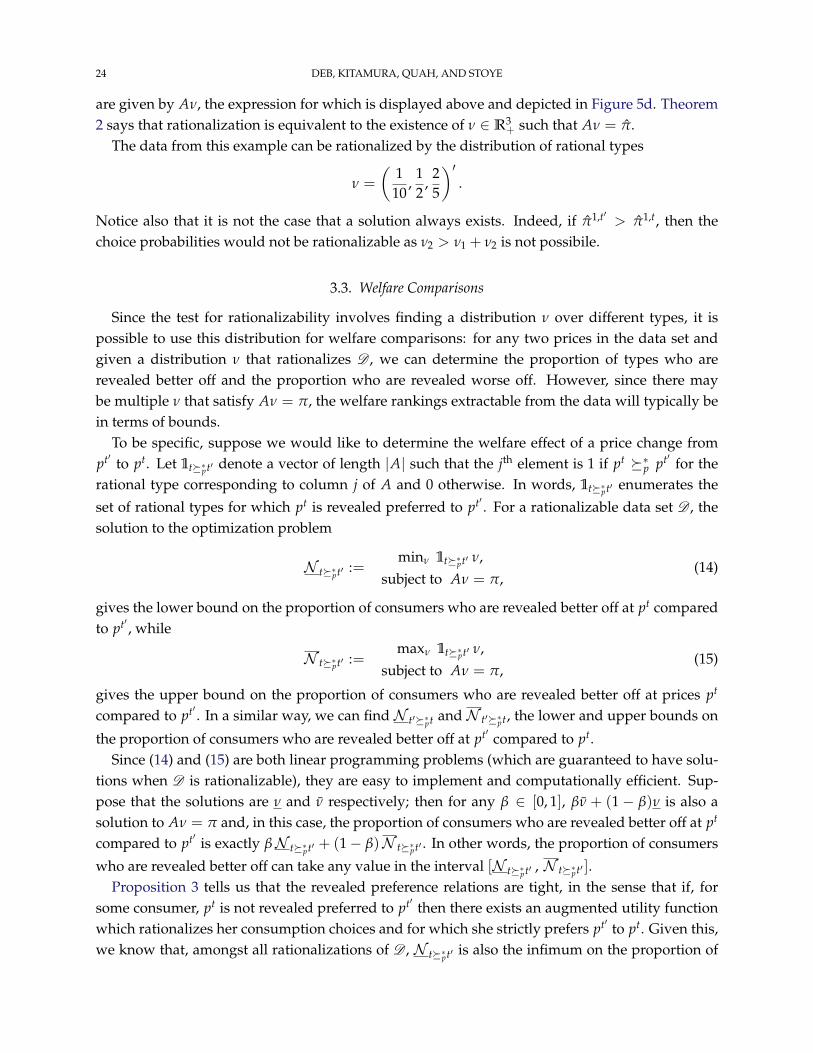
Since the test for rationalizability involves finding a distribution ν over different types, it ispossible to use this distribution for welfare comparisons: for any two prices in the data set andgiven a distribution ν that rationalizes D , we can determine the proportion of types who arerevealed better off and the proportion who are revealed worse off. However, since there maybe multiple ν that satisfy Aν = π, the welfare rankings extractable from the data will typically bein terms of bounds.
To be specific, suppose we would like to determine the welfare effect of a price change frompt′ to pt. Let 1t∗pt′ denote a vector of length |A| such that the jth element is 1 if pt ∗p pt′ for therational type corresponding to column j of A and 0 otherwise. In words, 1t∗pt′ enumerates the
set of rational types for which pt is revealed preferred to pt′ . For a rationalizable data set D , thesolution to the optimization problem
N t∗pt′ :=minν 1t∗pt′ ν,
subject to Aν = π,(14)
gives the lower bound on the proportion of consumers who are revealed better off at pt comparedto pt′ , while
N t∗pt′ :=maxν 1t∗pt′ ν,
subject to Aν = π,(15)
gives the upper bound on the proportion of consumers who are revealed better off at prices pt
compared to pt′ . In a similar way, we can find N t′∗pt and N t′∗pt, the lower and upper bounds on
the proportion of consumers who are revealed better off at pt′ compared to pt.Since (14) and (15) are both linear programming problems (which are guaranteed to have solu-
tions when D is rationalizable), they are easy to implement and computationally efficient. Sup-pose that the solutions are ν and ν respectively; then for any β ∈ [0, 1], βν + (1− β)ν is also asolution to Aν = π and, in this case, the proportion of consumers who are revealed better off at pt
compared to pt′ is exactly βN t∗pt′ + (1− β)N t∗pt′ . In other words, the proportion of consumers
who are revealed better off can take any value in the interval [N t∗pt′ , N t∗pt′ ].Proposition 3 tells us that the revealed preference relations are tight, in the sense that if, for
some consumer, pt is not revealed preferred to pt′ then there exists an augmented utility functionwhich rationalizes her consumption choices and for which she strictly prefers pt′ to pt. Given this,we know that, amongst all rationalizations of D , N t∗pt′ is also the infimum on the proportion of
REVEALED PRICE PREFERENCE 25
consumers who are better off at pt compared to pt′ . At the other extreme, we know that there is arationalization for which the proportion of consumers who are revealed better off at pt′ comparedto pt is as low as N t′∗pt.
16 Applying Proposition 3 again, a rationalization could be chosen such
that all other consumers prefer pt to pt′ . Therefore, across all rationalizations of D , 1−N t′∗pt is
the supremum on the proportion of consumers who prefer pt and pt′ .The following proposition summarizes these observations.
Proposition 4. Let D = (pt, πt)Tt=1 be a stochastic data set that satisfies Assumption A1 and is ratio-
nalized by the augmented utility model.
(i) Then for every η ∈ [N t∗pt′ , N t∗pt′ ], there is rationalization of D for which η is the proportion of
consumers who are revealed better off at pt compared to pt′ .(ii) For any rationalization of D , there is a proportion of consumers who are better off at pt compared to
pt′ ; let M be the set containing these proportions. Then inf M = N t∗pt′ and sup M = 1−N t′∗pt.
It may be helpful to consider how Proposition 4 applies to Example 3. In that case, there isa unique solution to Aν = π and the proportion of consumers who are revealed better off at pt
compared to pt′ is ν2 = 1/2, while the proportion who are revealed better off at pt′ to pt is ν3 = 2/5.Those consumers who belong to neither of these two types could be either better or worse at pt
compared to pt′ . Therefore, across all rationalizations of that data set, the proportion of consumerswho are better off at pt compared to pt′ can be as low as 1/2 and as high as 1− 2/5 = 3/5.
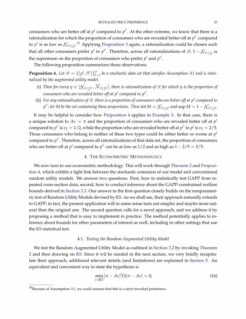
4. THE ECONOMETRIC METHODOLOGY
We now turn to our econometric methodology. This will work through Theorem 2 and Proposi-tion 4, which exhibit a tight link between the stochastic extension of our model and conventionalrandom utility models. We answer two questions: First, how to statistically test GAPP from re-peated cross-section data; second, how to conduct inference about the GAPP-constrained welfarebounds derived in Section 3.3. Our answer to the first question closely builds on the nonparamet-ric test of Random Utility Models devised by KS. As we shall see, their approach naturally extendsto GAPP; in fact, the present application will in some sense turn out simpler and maybe more nat-ural than the original one. The second question calls for a novel approach, and we address it byproposing a method that is easy to implement in practice. The method potentially applies to in-ference about bounds for other parameters of interest as well, including in other settings that usethe KS statistical test.
4.1. Testing the Random Augmented Utility Model
We test the Random Augmented Utility Model as outlined in Section 3.2 by invoking Theorem2 and then drawing on KS. Since it wil be needed in the next section, we very briefly recapitu-late their approach; additional relevant details (and limitations) are explained in Section 5. Anequivalent and convenient way to state the hypothesis is
minν∈RH
+
[π − Aν]′Ω[π − Aν] = 0, (16)
16Because of Assumption A1, we could assume that this is a strict revealed preference.

26 DEB, KITAMURA, QUAH, AND STOYE
where Ω is a positive definite matrix and H = |A|. The solution of the above minimizationproblem is the projection of π onto the cone
Aν : ν ∈ RH
+
under the weighted norm ‖x‖Ω =√
x′Ωx. The corresponding value of the objective function is the squared length of the projectionresidual vector. Of course, choice probabilities π can be rationalized by a random augmentedutility model if and only if the length of the residual vector is zero.
KS construct the following test statistic given by the natural sample counterpart of the objectivefunction (16):
JN := N minν∈RH
+
[π − Aν]′Ω[π − Aν], (17)
where π estimates the normalized and discretized choice probabilities π by the sample choicefrequencies (as in Figure 4c)17 and N denotes the total number of observations (the sum of thenumber of households across years). The normalization by N is done in order to obtain an appro-priate asymptotic distribution.
As we mentioned in the previous section, the minimizing value ν may not be unique but theresulting choice probabilities Aν are unique at the optimum. This latter term can be interpreted asa rationality-constrained estimator of choice probabilities. Note that Aν = π and JN = 0, iff thesample choice frequencies can be rationalized by a random augmented utility model. In this case,the null hypothesis is trivially accepted. KS devise a procedure to estimate the distribution of JN
in order to determine the appropriate critical value for the test statistic.
4.2. Estimating Welfare Bounds
We can test whether a particular number Nt∗pt′ is in the welfare bounds from Proposition 4 byadding a linear constraint to the hypothesis (16). Formally, we test
minν∈RH
+ , 1t∗pt′ ν=Nt∗pt′[π − Aν]′Ω[π − Aν] = 0 (18)
or equivalently, whether π is contained in the set
S(Nt∗pt′) = π = Aν|1′t∗pt′ν = Nt∗pt′ , ν ∈ ∆H−1,
where ∆H−1 is the H− 1-unit simplex; thus, the set collects all rationalizable vectors π compatiblewith the proportion Nt∗pt′ .
A confidence interval is generated by inverting the hypothesis test. The challenge is to computean appropriate critical value for this test statistic even though its limiting distribution discontinu-ously depends on nuisance parameters in a very complex manner.
Once again, the hypothesis being tested here takes the form
π ∈ S(Nt∗pt′). (19)
Later in this section, we prove that this is equivalent to
D(Nt∗pt′)π ≤ 0, (20)
17In the data we employ for our empirical application, there are no observations that lie on the intersection of any twonormalized budget sets so πt determines a probability measure on B1,t, . . . , BIt ,t.
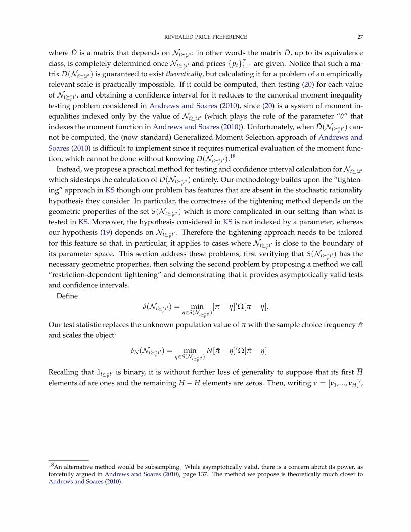
REVEALED PRICE PREFERENCE 27
where D is a matrix that depends on Nt∗pt′ : in other words the matrix D, up to its equivalenceclass, is completely determined once Nt∗pt′ and prices ptT
t=1 are given. Notice that such a ma-trix D(Nt∗pt′) is guaranteed to exist theoretically, but calculating it for a problem of an empiricallyrelevant scale is practically impossible. If it could be computed, then testing (20) for each valueof Nt∗pt′ , and obtaining a confidence interval for it reduces to the canonical moment inequalitytesting problem considered in Andrews and Soares (2010), since (20) is a system of moment in-equalities indexed only by the value of Nt∗pt′ (which plays the role of the parameter “θ” thatindexes the moment function in Andrews and Soares (2010)). Unfortunately, when D(Nt∗pt′) can-not be computed, the (now standard) Generalized Moment Selection approach of Andrews andSoares (2010) is difficult to implement since it requires numerical evaluation of the moment func-tion, which cannot be done without knowing D(Nt∗pt′).18
Instead, we propose a practical method for testing and confidence interval calculation forNt∗pt′
which sidesteps the calculation of D(Nt∗pt′) entirely. Our methodology builds upon the “tighten-ing” approach in KS though our problem has features that are absent in the stochastic rationalityhypothesis they consider. In particular, the correctness of the tightening method depends on thegeometric properties of the set S(Nt∗pt′) which is more complicated in our setting than what istested in KS. Moreover, the hypothesis considered in KS is not indexed by a parameter, whereasour hypothesis (19) depends on Nt∗pt′ . Therefore the tightening approach needs to be tailoredfor this feature so that, in particular, it applies to cases where Nt∗pt′ is close to the boundary ofits parameter space. This section address these problems, first verifying that S(Nt∗pt′) has thenecessary geometric properties, then solving the second problem by proposing a method we call“restriction-dependent tightening” and demonstrating that it provides asymptotically valid testsand confidence intervals.
Defineδ(Nt∗pt′) = min
η∈S(Nt∗pt′ )[π − η]′Ω[π − η].
Our test statistic replaces the unknown population value of π with the sample choice frequency π
and scales the object:
δN(Nt∗pt′) = minη∈S(Nt∗pt′ )
N[π − η]′Ω[π − η]
Recalling that 1t∗pt′ is binary, it is without further loss of generality to suppose that its first Helements of are ones and the remaining H − H elements are zeros. Then, writing ν = [ν1, ..., νH ]
′,
18An alternative method would be subsampling. While asymptotically valid, there is a concern about its power, asforcefully argued in Andrews and Soares (2010), page 137. The method we propose is theoretically much closer toAndrews and Soares (2010).

28 DEB, KITAMURA, QUAH, AND STOYE
and A = [A...A], A = [a1, ..., aH ], A = [aH+1, ..., aH ]
S(Nt∗pt′) = π = Aν|H
∑j=1
νj = Nt∗pt′ ,H
∑j=H+1
νj = 1−Nt∗pt′ , ν ∈ RH+
= π = Nt∗pt′π + (1−Nt∗pt′)π|π =H
∑j=1
νjaj, νj ≥ 0,
H
∑j=1
νj = 1, π =H−H
∑j′=1
νjaj′+H, νj′ ≥ 0,H
∑j′=1
νj′ = 1
= Nt∗pt′convA⊕ (1−Nt∗pt′)convA
where the ⊕ sign in the last line signifies Minkowski addition. By a basic property of Minkowskiaddition (e.g. Lemma 2 of Arrow and Hahn, 1971, p.387)
S(Nt∗pt′) = conv(Nt∗pt′a1, ...,Nt∗pt′aH ⊕ (1−Nt∗pt′))aH+1, ..., (1−Nt∗pt′))aH
).
Let e1, ..., eK, K ≤ H(H − H), be the collection of elements in Nt∗pt′a1, ...,Nt∗pt′aH ⊕ (1−Nt∗pt′))aH+1, ..., (1−Nt∗pt′))aH and E = [e1, ..., eK], then
S(Nt∗pt′) = conv(E),
or,S(Nt∗pt′) = cone(E) ∩ H,
where
H = π : 1′|π|π = T, I := |π| =T
∑t=1
It.
The following result provides an alternative representation that is useful for theoretical devel-opments of our statistical testing procedure.
Theorem 3. (Weyl-Minkowski Theorem for Cones) A subset C of RI is a finitely generated cone
C = ν1e1 + ... + νKeK : νh ≥ 0 for some E = [e1, ..., eK] ∈ RI×K (21)
if and only if it is a finite intersection of closed half spaces
C = t ∈ RI |Dt ≤ 0 for some D ∈ Rm×I . (22)
The expressions in (21) and (22) are called a V-representation (as in “vertices”) and aH-representation (asin “half spaces”) of C, respectively.
See, for example, Theorem 1.3 in Ziegler (1995).19
In what follows we use an H representation of cone(E) represented by a m × |π| matrix Das implied by Theorem 3. The following assumptions are used for our asymptotic theory. Letdi,t
n(t) = 1 if the n(t)-th consumer in the t-th crosssection chooses patch Bi,t, and di,tn(t) = 0 if she
does not. Define dtn(t) = [d1,t
n(t), ..., dIt,tn(t)].
19See Gruber (2007), Grunbaum, Kaibel, Klee, and Ziegler (2003) and Ziegler (1995) for these results and other materialsconcerning convex polytopes used in this paper.
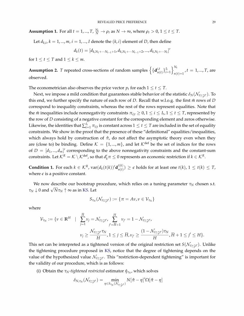
REVEALED PRICE PREFERENCE 29
Assumption 1. For all t = 1, ..., T, NtN → ρt as N → ∞, where ρt > 0, 1 ≤ t ≤ T.
Let dk,i, k = 1, ..., m, i = 1, ..., I denote the (k, i) element of D, then define
dk(t) = [dk,N1+···Nt−1+1, dk,N1+···Nt−1+2, ..., dk,N1+···Nt ]′
for 1 ≤ t ≤ T and 1 ≤ k ≤ m.
Assumption 2. T repeated cross-sections of random samplesdi,t
n(t)Iti=1
Nt
n(t)=1, t = 1, ..., T, are
observed.
The econometrician also observes the price vector pt for each 1 ≤ t ≤ T.Next, we impose a mild condition that guarantees stable behavior of the statistic δN(Nt∗pt′). To
this end, we further specify the nature of each row of D. Recall that w.l.o.g. the first m rows of Dcorrespond to inequality constraints, whereas the rest of the rows represent equalities. Note thatthe m inequalities include nonnegativity constraints πi|t ≥ 0, 1 ≤ i ≤ It, 1 ≤ t ≤ T, represented bythe row of D consisting of a negative constant for the corresponding element and zeros otherwise.Likewise, the identities that ∑It
i=1 πi|t is constant across 1 ≤ t ≤ T are included in the set of equalityconstraints. We show in the proof that the presence of these “definitional” equalities/inequalities,which always hold by construction of π, do not affect the asymptotic theory even when theyare (close to) be binding. Define K = 1, ..., m, and let Kdef be the set of indices for the rowsof D = [d1, ..., dm]′ corresponding to the above nonnegativity constraints and the constant-sumconstraints. Let KR = K \ Kdef, so that d′kπ ≤ 0 represents an economic restriction if k ∈ KR.
Condition 1. For each k ∈ KR, var(dk(t(k))′dt(k)n(t)) ≥ ε holds for at least one t(k), 1 ≤ t(k) ≤ T,
where ε is a positive constant.
We now describe our bootstrap procedure, which relies on a tuning parameter τN chosen s.t.τN ↓ 0 and
√NτN ↑ ∞ as in KS. Let
SτN (Nt∗pt′) := π = Aν, ν ∈ VτN
where
VτN := ν ∈ RH |H
∑j=1
νj = Nt∗pt′ ,H
∑j′=H+1
νj′ = 1−Nt∗pt′ ,
νj ≥Nt∗pt′τN
H, 1 ≤ j ≤ H, νj′ ≥
(1−Nt∗pt′)τN
H, H + 1 ≤ j′ ≤ H.
This set can be interpreted as a tightened version of the original restriction set S(Nt∗pt′). Unlikethe tightening procedure proposed in KS, notice that the degree of tightening depends on thevalue of the hypothesized value Nt∗pt′ . This “restriction-dependent tightening” is important forthe validity of our procedure, which is as follows:
(i) Obtain the τN-tightened restricted estimator ητN , which solves
δN,τN (Nt∗pt′) = minη∈SτN (Nt∗pt′ )
N[π − η]′Ω[π − η]

30 DEB, KITAMURA, QUAH, AND STOYE
(ii) Define the τN-tightened recentered bootstrap estimators
π∗(r)τN := π∗(r) − π + ητN , r = 1, ..., R.
(iii) The bootstrap test statistic is
δ∗(r)N,τN
(Nt∗pt′) = minη∈SτNNt∗pt′
N[π∗(r)τN − η]′Ω[π
∗(r)τN − η]
for r = 1, ..., R.(iv) Use the empirical distribution of δ
∗(r)N,τN
(Nt∗pt′), r = 1, ..., R to obtain the critical value forJN .
Note that the distribution of observations is uniquely characterized by the vector π. Let Pdenote the set of all π’s that satisfy Condition 1 for some (common) value of ε.
Theorem 4. Choose τN so that τN ↓ 0 and√
NτN ↑ ∞. Also, let Ω be diagonal, where all the diagonalelements are positive. Then under Assumptions 1 and 2
lim infN→∞
infπ∈P∩C
PrδN(Nt∗pt′) ≤ c1−α = 1− α
where c1−α is the 1− α quantile of δ∗N,τN, 0 ≤ α ≤ 1
2 .
Proof. Note
SτN (Nt∗pt′) = π = Aν :H
∑j=1
νj = Nt∗pt′ ,H
∑j′=H+1
νj′ = 1−Nt∗pt′ ,
νj ≥Nt∗pt′τN
H, 1 ≤ j ≤ H, νj′ ≥
(1−Nt∗pt′)τN
H, H + 1 ≤ j′ ≤ H.
Define
νj :=
νj
Nt∗pt′− τN
H
1−τn1 ≤ j ≤ H
νjNt∗pt′
− τNH
1−τnH + 1 ≤ j ≤ H,
then
SτN (Nt∗pt′) = π = Nt∗pt′
[(1− τN)
H
∑j=1
νjaj +τN
HA1H
]+ (1−Nt∗pt′)
(1− τN)H
∑j=H
νjaj +τN
HA1H
:
H
∑j=1
νj =H
∑j′=H+1
νj′ = 1, νj ≥ 0, 1 ≤ j ≤ H, νj′ ≥ 0, H + 1 ≤ j′ ≤ H
= Nt∗pt′[(1− τN)convA⊕ τN
HA1H
]+ (1−Nt∗pt′)
[(1− τN)convA⊕ τN
HA1H
]= (1− τN)conv
(Nt∗pt′a1, ...,Nt∗pt′aH ⊕ (1−Nt∗pt′))aH+1, ..., (1−Nt∗pt′))aH
)⊕τN
H
[Nt∗pt′A1H + (1−Nt∗pt′)A1H
]= (1− τN)conv(E)⊕ τN
H
[Nt∗pt′A1H + (1−Nt∗pt′)A1H
]

REVEALED PRICE PREFERENCE 31
For cone(E) letπ : Dπ ≤ 0
be its H-representation with D ∈ Rm×|π| such that, as Lemma 4.1 in KS , D =
[D≤
D=
], where
the submatrices D≤ ∈ Rm×|π| and D= ∈ R(m−m)×|π| correspond to inequality and equality con-straints, respectively.
SτN (Nt∗pt′) =(
cone(E)⊕ τN
H
[Nt∗pt′A1H + (1−Nt∗pt′)A1H
])∩ ∆H−1
= π ∈ R|π| : π − τN
H
[Nt∗pt′A1H + (1−Nt∗pt′)A1H
]∈ cone(E) ∩ ∆H−1
= p ∈ ∆T−1 : D[
p− τN
H
[Nt∗pt′A1H + (1−Nt∗pt′)A1H
]]≤ 0
= p ∈ ∆T−1 : Dp ≤ −τNφ,
whereφ = − 1
HD[Nt∗pt′A1H + (1−Nt∗pt′)A1H
].
for some φ = (φ1, ..., φm)′ satisifies (i) φ := [φ1, ..., φm]′ ∈ Rm++, and (ii) φk = 0 for k > m. Using the
above notation for theH-representation of cone(E),
δN(Nt∗pt′) = minπ∈∆T−1:Dπ≤0
N[π − π]′Ω[π − π].
As in KS , define ` = rank(D), and let `×m matrix K such that KD is a matrix whose rows consistof a basis of the row space row(D). Also let M be an (|π| − `)× |π| matrix whose rows form anorthonormal basis of kerD = ker(KD), and define P = (KD
M ). Finally, let g = Dπ.Unlike KS , we need to augment D with a row vector of ones to properly account for the con-
straint π ∈ ∆T−1:
D∗ :=(
D[1, ..., 1]
).
Define
T(x, y) =(
xy
)′P−1′ΩP−1
(xy
), x ∈ R`, y ∈ R|π|−`,
andt(x) := min
y∈R|π|−`T(x, y), s(g) := min
γ=[γ≤′,γ= ′]′,γ≤≤0,γ==0,[γ′,1]′∈col(D∗)t(K[g− γ]).
It is easy to see that t : R` → R+ is a positive definite quadratic form. We can write
δN(Nt∗pt′) = N minγ=[γ≤′,γ= ′]′,γ≤≤0,γ==0,[γ′,1]′∈col(D∗)
t(K[g− γ])
= Ns(g)
= s(√
Ng).

32 DEB, KITAMURA, QUAH, AND STOYE
Likewise, for the bootsgtrapped version of δ we have
δ∗N,τN(Nt∗pt′) = N min
γ=[γ≤′,γ= ′]′,γ≤≤0,γ==0,[γ′,1]′∈col(D∗)t(K[g− γ])
= Ns(g)
= s(ϕτN (ξ) +√
N[π∗ − π]).
where ξ = Dπ/τN . The function ϕN(ξ) = [ϕ1N(ξ), ..., ϕm
N(ξ)] for ξ = (ξ1, ..., ξm)′ ∈ col(D), thennoting that each elements ej, 1 ≤ j ≤ K that defines cone(E) takes the form Nt∗pt′ah + (1 −Nt∗pt′))ao, 1 ≤ h ≤ H, H + 1 ≤ o ≤ H, by the proof of Theorem 4.2 of KS , it follows that itsk-th element ϕk
N for k ≤ m satisfiesϕk
N(ξ) = 0
if |ξk| ≤ δ and ξ j ≤ δ, 1 ≤ j ≤ m, δ > 0, for large enough N and ϕkN(ξ) = 0 for k > m. The
conclusion follows by Theorem 1 of Andrews and Soares (2010).
Theorem 4 is concerned with the validity of our bootstrap procedure concerning the restrictionof the form 1t∗pt′ν = Nt∗pt′ . While our specific structure is useful and instructive (e.g. it allowsus to provide a concrete characterization of the matrix E, which provides S(Nt∗pt′) = conv(E), asdiscussed above) the above procedure generalizes to a general restriction of the formRν = c,R ∈Rr×H, c ∈ Rr, once the tightening procedure is tailored appropriately to accommodate the generalform. This extension is to be discussed in a subsequent version of the paper.
The crucial step in our procedure is that tightening turns non-binding inequalities in the H-representation with small slack into binding ones but not vice versa. This feature is not universal,but it is guaranteed to work when the restriction polytope for π (S(Nt∗pt′) in the current appli-cation) satisfies a certain condition (loosely speaking, when corners of the polytope are acute),provided that the econometrician chooses Ω to be diagonal.
5. EMPIRICAL APPLICATION (PRELIMINARY!)
We implement a test of stochastic GAPP on the 1975-1999 waves of the U.K. Family ExpenditureSurvey, a repeated cross-section of consumption data with reasonably high resolution. These dataare a staple of the nonparametric demand literature: Blundell, Browning, and Crawford (2008), KSand Adams (2016) use the exact same data selection and in that sense are exact comparables to ourimplementation; Hoderlein and Stoye (2014), Kawaguchi (2017), and others also draw on the samedata set. To reduce covariate variability, we restrict attention to households with cars and kids.We do not smooth data in any form: All data points are projected onto a fictitious expenditure of 1as in Figure 5d, and choice probabilities are then estimated by corresponding sample frequencies.Computation of critical values and p-values for the test uses the ”cone tightening” procedureproposed by KS and thereby is valid uniformly asymptotically over a large range of underlyingparameter values.20
20In particular, since we literally use sample frequencies as estimators of probabilities, the somewhat simpler assump-tions of Section 4 in KS suffice.
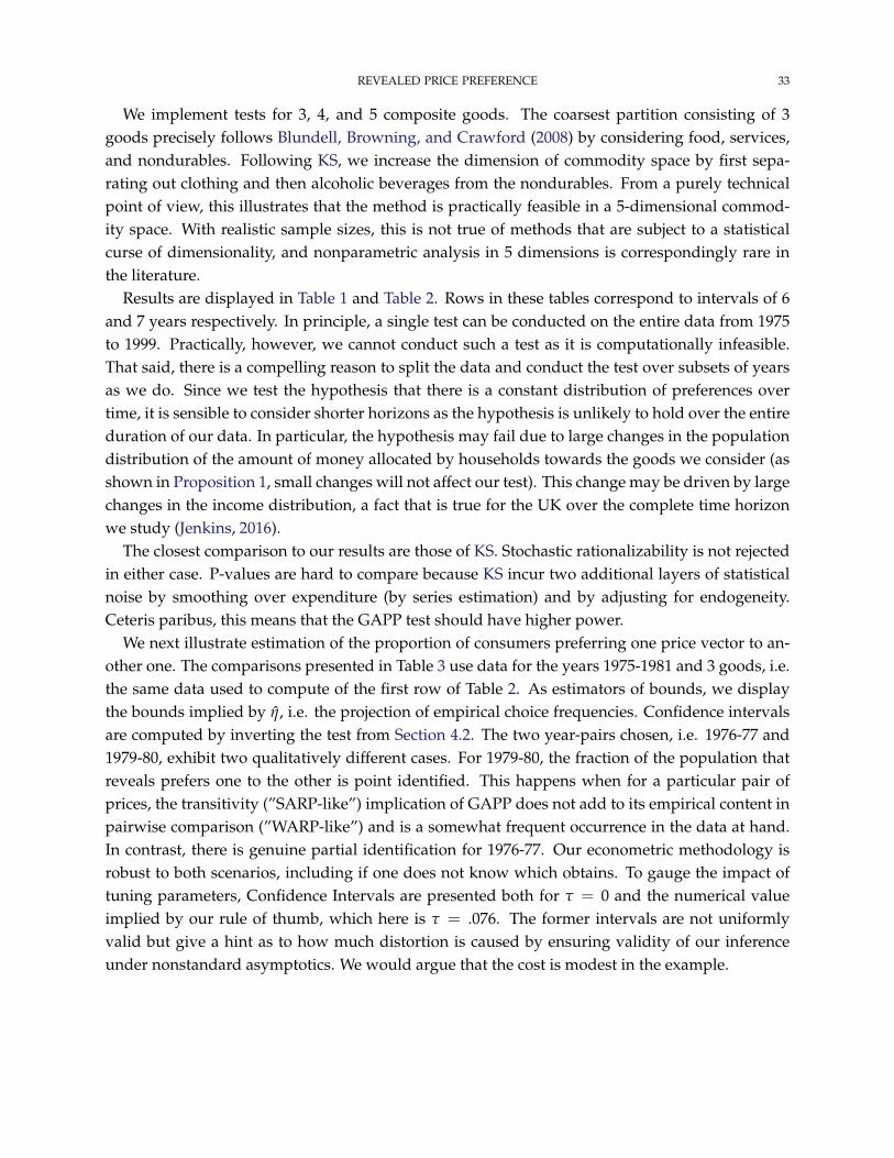
REVEALED PRICE PREFERENCE 33
We implement tests for 3, 4, and 5 composite goods. The coarsest partition consisting of 3goods precisely follows Blundell, Browning, and Crawford (2008) by considering food, services,and nondurables. Following KS, we increase the dimension of commodity space by first sepa-rating out clothing and then alcoholic beverages from the nondurables. From a purely technicalpoint of view, this illustrates that the method is practically feasible in a 5-dimensional commod-ity space. With realistic sample sizes, this is not true of methods that are subject to a statisticalcurse of dimensionality, and nonparametric analysis in 5 dimensions is correspondingly rare inthe literature.
Results are displayed in Table 1 and Table 2. Rows in these tables correspond to intervals of 6and 7 years respectively. In principle, a single test can be conducted on the entire data from 1975to 1999. Practically, however, we cannot conduct such a test as it is computationally infeasible.That said, there is a compelling reason to split the data and conduct the test over subsets of yearsas we do. Since we test the hypothesis that there is a constant distribution of preferences overtime, it is sensible to consider shorter horizons as the hypothesis is unlikely to hold over the entireduration of our data. In particular, the hypothesis may fail due to large changes in the populationdistribution of the amount of money allocated by households towards the goods we consider (asshown in Proposition 1, small changes will not affect our test). This change may be driven by largechanges in the income distribution, a fact that is true for the UK over the complete time horizonwe study (Jenkins, 2016).
The closest comparison to our results are those of KS. Stochastic rationalizability is not rejectedin either case. P-values are hard to compare because KS incur two additional layers of statisticalnoise by smoothing over expenditure (by series estimation) and by adjusting for endogeneity.Ceteris paribus, this means that the GAPP test should have higher power.
We next illustrate estimation of the proportion of consumers preferring one price vector to an-other one. The comparisons presented in Table 3 use data for the years 1975-1981 and 3 goods, i.e.the same data used to compute of the first row of Table 2. As estimators of bounds, we displaythe bounds implied by η, i.e. the projection of empirical choice frequencies. Confidence intervalsare computed by inverting the test from Section 4.2. The two year-pairs chosen, i.e. 1976-77 and1979-80, exhibit two qualitatively different cases. For 1979-80, the fraction of the population thatreveals prefers one to the other is point identified. This happens when for a particular pair ofprices, the transitivity (”SARP-like”) implication of GAPP does not add to its empirical content inpairwise comparison (”WARP-like”) and is a somewhat frequent occurrence in the data at hand.In contrast, there is genuine partial identification for 1976-77. Our econometric methodology isrobust to both scenarios, including if one does not know which obtains. To gauge the impact oftuning parameters, Confidence Intervals are presented both for τ = 0 and the numerical valueimplied by our rule of thumb, which here is τ = .076. The former intervals are not uniformlyvalid but give a hint as to how much distortion is caused by ensuring validity of our inferenceunder nonstandard asymptotics. We would argue that the cost is modest in the example.
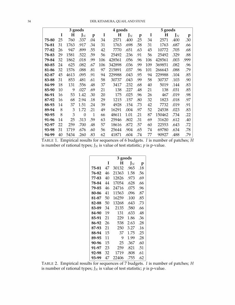
34 DEB, KITAMURA, QUAH, AND STOYE
3 goods 4 goods 5 goodsI H JN p I H JN p I H JN p
75-80 25 760 .337 .04 34 2571 .400 .25 34 2571 .400 .3076-81 31 1763 .917 .34 31 1763 .698 .58 31 1763 .687 .6677-82 26 947 .899 .55 42 7770 .651 .63 45 10772 .705 .6878-83 29 1581 .522 .59 56 25492 .236 .91 56 25492 .329 .8879-84 32 1862 .018 .99 106 428561 .056 .96 106 428561 .003 .99980-85 24 625 .082 .67 106 342898 .036 .99 109 369851 .082 .9681-86 32 1576 .088 .81 97 215891 .037 .96 101 266643 .088 .7982-87 45 4613 .095 .91 94 229988 .043 .95 94 229988 .104 .8583-88 31 853 .481 .61 58 30737 .043 .99 58 30737 .103 .9084-99 18 131 .556 .48 37 3417 .232 .68 40 5019 .144 .8385-90 10 9 .027 .69 21 138 .227 .48 21 138 .031 .8586-91 16 53 1.42 .30 20 175 .025 .96 26 467 .019 .9887-92 16 68 2.94 .18 29 1215 .157 .80 32 1823 .018 .9788-93 14 37 1.51 .24 39 4928 .154 .73 42 7732 .019 .9189-94 8 3 1.72 .21 49 16291 .004 .97 52 24538 .023 .8390-95 8 3 0 1 66 48611 1.01 .21 87 150462 .734 .2291-96 14 25 .313 .59 63 25946 .802 .31 69 31620 .612 .4092-97 22 259 .700 .48 57 18616 .872 .57 60 22553 .643 .7293-98 31 1719 .676 .60 56 25644 .904 .65 74 69780 .634 .7894-99 40 5434 .260 .83 62 41871 .604 .74 77 90927 .488 .79
TABLE 1. Empirical results for sequences of 6 budgets. I is number of patches; His number of rational types; JN is value of test statistic; p is p-value.
3 goodsI H JN p
75-81 47 30132 .965 .1876-82 46 21363 1.58 .5677-83 40 12826 .973 .6978-84 44 17054 .628 .6679-85 46 24716 .075 .9680-86 41 11563 .096 .8781-87 50 16259 .100 .8582-88 50 13268 .643 .7383-89 34 2135 .580 .6684-90 19 131 .633 .4885-91 21 229 1.86 .3686-92 26 538 2.63 .2887-93 21 250 3.27 .1688-94 15 37 1.75 .2589-95 11 9 1.99 .2890-96 15 25 .367 .6091-97 23 259 .821 .5192-98 32 1719 .808 .6193-99 47 22406 .755 .62
TABLE 2. Empirical results for sequences of 7 budgets. I is number of patches; His number of rational types; JN is value of test statistic; p is p-value.

REVEALED PRICE PREFERENCE 35
comparison estimated bounds CI, τ = 0 CI, τ = .076p1977 p1976 [.119, .137] [.102, .149] [.094, .168]p1976 p1977 [.843, .883] [.827, .897] [.821, .904]p1980 p1979 .498 [.471, .524] [.469, .526]p1979 p1980 .464 [.436, .491] [.432, .495]
TABLE 3. Estimated bounds and Confidence Intervals for proportion of consumerspreferring one price to another one. Data used are for 1975 − 1981. Confidenceintervals for τ = 0 are not expected to be valid but are reported to gauge the con-servative distortion due to uniform inference.
6. CONCLUSION
We developed a revealed preference analysis of a model of consumption in which the consumermaximizes utility over an observed set of purchases, taking into account a disutility of expendi-ture, but is not subjected to a hard budget constraint (in particular, the model generalizes quasi-linear utility). As our analysis shows, this model has bite in consumer choice settings where totalexpenditure is unobserved (as the data only contains information on a subset of the goods).
A useful aspect of the model is that it easily generalizes to a random utility context that arisesnaturally in demand analysis using repeated cross-section data but avoiding restrictions on unob-served heterogeneity. For such a setting, we show how to statistically test the model and also howto do (partially identified) welfare analysis, e.g. inference on the proportion of a population thatbenefit from a price change. This is illustrated with U.K. Family Expenditure Survey data. Themodel is not rejected, and bounds are informative. Further empirical applications are in progress.

36 DEB, KITAMURA, QUAH, AND STOYE
REFERENCES
ADAMS, A. (2016): “Mutually consistent revealed preference bounds,” Manuscript, University ofOxford.
AFRIAT, S. N. (1967): “The Construction of Utility Functions from Expenditure Data,” InternationalEconomic Review, 8(1), 67–77.
ANDREWS, D. W., AND G. SOARES (2010): “Inference for Parameters Defined by Moment Inequal-ities Using Generalized Moment Selection,” Econometrica, 78, 119–157.
ARROW, K. J., AND F. HAHN (1971): General competitive analysis. Holden-Day.BLUNDELL, R., M. BROWNING, AND I. CRAWFORD (2008): “Best Nonparametric Bounds on De-
mand Responses,” Econometrica, 76(6), 1227–1262.BLUNDELL, R., J. L. HOROWITZ, AND M. PAREY (2012): “Measuring the Price Responsiveness
of Gasoline Demand: Economic Shape Restrictions and Nonparametric Demand Estimation,”Quantitative Economics, 3(1), 29–51.
BROWN, D. J., AND C. CALSAMIGLIA (2007): “The Nonparametric Approach to Applied WelfareAnalysis,” Economic Theory, 31(1), 183–188.
CRAWFORD, I., AND B. DE ROCK (2014): “Empirical Revealed Preference,” Annual Review of Eco-nomics, 6(1), 503–524.
FORGES, F., AND E. MINELLI (2009): “Afriat’s Theorem for General Budget Sets,” Journal of Eco-nomic Theory, 144(1), 135–145.
FOSTEL, A., H. E. SCARF, AND M. J. TODD (2004): “Two New Proofs of Afriats Theorem,” Eco-nomic Theory, 24(1), 211–219.
GRUBER, P. (2007): Convex and Discrete Geometry, Grundlehren der mathematischen Wis-senschaften. Springer, New York.
GRUNBAUM, B., V. KAIBEL, V. KLEE, AND G. M. ZIEGLER (2003): Convex polytopes. Springer, NewYork.
HAUSMAN, J. A., AND W. K. NEWEY (2016): “Individual Heterogeneity and Average Welfare,”Econometrica, 84(3), 1225–1248.
HODERLEIN, S., AND J. STOYE (2014): “Revealed Preferences in a Heterogeneous Population,” TheReview of Economics and Statistics, 96(2), 197–213.
JENKINS, S. P. (2016): “The Income Distribution in the UK,” in Social Advantage and Disadvantage,ed. by H. Dean, and L. Platt, pp. 135–160. Oxford University Press.
KAWAGUCHI, K. (2017): “Testing rationality without restricting heterogeneity,” Journal of Econo-metrics, 197(1), 153 – 171.
KITAMURA, Y., AND J. STOYE (2013): “Nonparametric Analysis of Random Utility Models: Test-ing,” Cowles Foundation Discussion Paper.
MCFADDEN, D. L., AND M. K. RICHTER (1991): “Stochastic Rationality and Revealed StochasticPreference,” in Preferences, Uncertainty and Rationality, ed. by D. M. J. Chipman, and M. Richter.Boulder: Westview Press.
QUAH, J. K.-H. (2014): “A Test for Weakly Separable Preferences,” Oxford University DiscussionPaper.

REVEALED PRICE PREFERENCE 37
SCHWARTZ, M. (1990): “Third-Degree Price Discrimination and Output: Generalizing a WelfareResult,” American Economic Review, 80(5), 1259–1262.
THALER, R. H. (1999): “Mental Accounting Matters,” Journal of Behavioral Decision Making, 12(3),183–206.
VARIAN, H. R. (1982): “The Nonparametric Approach to Demand Analysis,” Econometrica, 50(4),945–973.
(1985): “Price Discrimination and Social Welfare,” American Economic Review, 75(4), 870–875.
VARIAN, H. R. (1988): “Revealed Preference with a Subset of Goods,” Journal of Economic Theory,46(1), 179–185.
ZIEGLER, G. M. (1995): Lectures on polytopes, Graduate texts in mathematics. Springer, New York.