arX

iv:c

s/03

1203

8v1

[cs

.AI]

17

Dec

200

3

Responsibility and Blame: A Structural-Model

Approach

Hana ChocklerSchool of Engineering and Computer Science

Hebrew University

Jerusalem 91904, Israel.Email: hanac@cs.huji.ac.il

Joseph Y. Halpern∗

Department of Computer ScienceCornell University

Ithaca, NY 14853, U.S.A.Email: halpern@cs.cornell.edu

November 8, 2018

Abstract

Causality is typically treated an all-or-nothing concept; either A is a cause ofB or it is not. We extend the definition of causality introduced by Halpern andPearl [2001a] to take into account the degree of responsibility of A for B. Forexample, if someone wins an election 11–0, then each person who votes for him isless responsiblefor the victory than if he had won 6–5. We then define a notionof degree of blame, which takes into account an agent’s epistemic state. Roughlyspeaking, the degree of blame of A for B is the expected degree of responsibility ofA for B, taken over the epistemic state of an agent.

∗Supported in part by NSF under grant CTC-0208535 and by the DoD Multidisciplinary UniversityResearch Initiative (MURI) program administered by ONR under grant N00014-01-1-0795.

1 Introduction

There have been many attempts to define causality going back to Hume [1739], andcontinuing to the present (see, for example, [Collins, Hall, and Paul 2003; Pearl 2000] forsome recent work). While many definitions of causality have been proposed, all of themtreat causality is treated as an all-or-nothing concept. That is, A is either a cause of B orit is not. As a consequence, thinking only in terms of causality does not at times allow usto make distinctions that we may want to make. For example, suppose that Mr. B winsan election against Mr. G by a vote of 11–0. Each of the people who voted for Mr. B isa cause of him winning. However, it seems that their degree of responsibility should notbe as great as in the case when Mr. B wins 6–5.

In this paper, we present a definition of responsibility that takes this distinction intoaccount. The definition is an extension of a definition of causality introduced by Halpernand Pearl [2001a]. Like many other definitions of causality going back to Hume [1739],this definition is based on counterfactual dependence. Roughly speaking, A is a causeof B if, had A not happened (this is the counterfactual condition, since A did in facthappen) then B would not have happened. As is well known, this naive definition doesnot capture all the subtleties involved with causality. (If it did, there would be far fewerpapers in the philosophy literature!) In the case of the 6–5 vote, it is clear that, accordingto this definition, each of the voters for Mr. B is a cause of him winning, since if they hadvoted against Mr. B, he would have lost. On the other hand, in the case of the 11-0 vote,there are no causes according to the naive counterfactual definition. A change of one votedoes not makes no difference. Indeed, in this case, we do say in natural language that thecause is somewhat “diffuse”.

While in this case the standard counterfactual definition may not seem quite so prob-lematic, the following example (taken from [Hall 2003]) shows that things can be evenmore subtle. Suppose that Suzy and Billy both pick up rocks and throw them at a bottle.Suzy’s rock gets there first, shattering the bottle. Since both throws are perfectly accu-rate, Billy’s would have shattered the bottle had Suzy not thrown. Thus, according tothe naive counterfactual definition, Suzy’s throw is not a cause of the bottle shattering.This certainly seems counter to intuition.

Both problems are dealt with the same way in [Halpern and Pearl 2001a]. Roughlyspeaking, the idea is that A is a cause of B if B counterfactually depends on C under somecontingency. For example, voter 1 is a cause of Mr. B winning even if the vote is 11–0because, under the contingency that 5 of the other voters had voted for Mr. G instead,voter 1’s vote would have become critical; if he had then changed his vote, Mr. B wouldnot have won. Similarly, Suzy’s throw is the cause of the bottle shattering because thebottle shattering counterfactually depends on Suzy’s throw, under the contingency thatBilly doesn’t throw. (There are further subtleties in the definition that guarantee that,if things are modeled appropriately, Billy’s throw is not a cause. These are discussed inSection 2.)

It is precisely this consideration of contingencies that lets us define degree of respon-

1

sibility. We take the degree of responsibility of A for B to be 1/(N + 1), where N is theminimal number of changes that have to be made to obtain a contingency where B coun-terfactually depends on A. (If A is not a cause of B, then the degree of responsibility is 0.)In particular, this means that in the case of the 11–0 vote, the degree of responsibility ofany voter for the victory is 1/6, since 5 changes have to be made before a vote is critical.If the vote were 1001–0, the degree of responsibility of any voter would be 1/501. On theother hand, if the vote is 5–4, then the degree of responsibility of each voter for Mr. B forMr. B’s victory is 1; each voter is critical. As we would expect, those voters who votedfor Mr. G have degree of responsibility 0 for Mr. B’s victory, since they are not causes ofthe victory. Finally, in the case of Suzy and Billy, even though Suzy is the only cause ofthe bottle shattering, Suzy’s degree of responsibility is 1/2, while Billy’s is 0. Thus, thedegree of responsibility measures to some extent whether or not there are other potentialcauses.

When determining responsibility, it is assumed that everything relevant about thefacts of the world and how the world works (which we characterize in terms of what arecalled structural equations) is known. For example, when saying that voter 1 has degreeof responsibility 1/6 for Mr. B’s win when the vote is 11–0, we assume that the vote andthe procedure for determining a winner (majority wins) is known. There is no uncertaintyabout this. Just as with causality, there is no difficulty in talking about the probabilitythat someone has a certain degree of responsibility by putting a probability distribution onthe way the world could be and how it works. But this misses out on important componentof determining what we call here blame: the epistemic state. Consider a doctor who treatsa patient with a particular drug resulting in the patient’s death. The doctor’s treatmentis a cause of the patient’s death; indeed, the doctor may well bear degree of responsibility1 for the death. However, if the doctor had no idea that the treatment had adverse sideeffects for people with high blood pressure, he should perhaps not be held to blame for thedeath. Actually, in legal arguments, it may not be so relevant what the doctor actuallydid or did not know, but what he should have known. Thus, rather than considering thedoctor’s actual epistemic state, it may be more important to consider what his epistemicstate should have been. But, in any case, if we are trying to determine whether the doctoris to blame for the patient’s death, we must take into account the doctor’s epistemic state.

We present a definition of blame that considers whether agent a performing action bis to blame for an outcome ϕ. The definition is relative to an epistemic state for a, whichis taken, roughly speaking, to be a set of situations before action b is performed, togetherwith a probability on them. The degree of blame is then essentially the expected degreeof responsibility of action b for ϕ (except that we ignore situations where ϕ was alreadytrue or b was already performed). To understand the difference between responsibility andblame, suppose that there is a firing squad consisting of ten excellent marksmen. Onlyone of them has live bullets in his rifle; the rest have blanks. The marksmen do not knowwhich of them has the live bullets. The marksmen shoot at the prisoner and he dies. Theonly marksman that is the cause of the prisoner’s death is the one with the live bullets.That marksman has degree of responsibility 1 for the death; all the rest have degree of

2

responsibility 0. However, each of the marksmen has degree of blame 1/10.1

While we believe that our definitions of responsibility and blame are reasonable, theycertainly do not capture all the connotations of these words as used in the literature.In the philosophy literature, papers on responsibility typically are concerned with moralresponsibility (see, for example, [Zimmerman 1988]). Our definitions, by design, do nottake into account intentions or possible alternative actions, both of which seem necessaryin dealing with moral issues. For example, there is no question that Truman was inpart responsible and to blame for the deaths resulting from dropping the atom bombson Hiroshima and Nagasaki. However, to decide whether this is a morally reprehensibleact, it is also necessary to consider the alternative actions he could have performed, andtheir possible outcomes. While our definitions do not directly address these moral issues,we believe that they may be helpful in elucidating them. Shafer [2001] discusses a notionof responsibility that seems somewhat in the spirit of our notion of blame, especially inthat he views responsibility as being based (in part) on causality. However, he does notgive a formal definition of responsibility, so it is hard to compare our definitions to his.However, there are some significant technical differences between his notion of causality(discussed in [Shafer 1996]) and that on which our notions are based. We suspect thatany notion of responsibility or blame that he would define would be different from ours.We return to these issues in Section 5.

The rest of this paper is organized as follows. In Section 2 we review the basic defini-tions of causal models based on structural equations, which are the basis for our defini-tions of responsibility and blame. In Section 3, we review the definition of causality from[Halpern and Pearl 2001a], and show how it can be modified to give a definition of respon-sibility. We show that the definition of responsibility gives reasonable answer in a numberof cases, and briefly discuss how it can be used in program verification (see [Chockler,Halpern, and Kupferman 2003]). In Section 3.3, we give our definition of blame. In Sec-tion 4, we discuss the complexity of computing responsibility and blame. We conclude inSection 5 with some discussion of responsibility and blame.

2 Causal Models: A Review

In this section, we review the details of the definitions of causal models from [Halpernand Pearl 2001a]. This section is essentially identical to the corresponding section in[Chockler, Halpern, and Kupferman 2003]; the material is largely taken from [Halpernand Pearl 2001a].

A signature is a tuple S = 〈U ,V,R〉, where U is a finite set of exogenous variables,V is a set of endogenous variables, and R associates with every variable Y ∈ U ∪ V anonempty set R(Y ) of possible values for Y . Intuitively, the exogenous variables are oneswhose values are determined by factors outside the model, while the endogenous variables

1We thank Tim Williamson for this example.

3

are ones whose values are ultimately determined by the exogenous variables. A causalmodel over signature S is a tuple M = 〈S,F〉, where F associates with every endogenousvariable X ∈ V a function FX such that FX : (×U∈UR(U)× (×Y ∈V\{X}R(Y )))→ R(X).That is, FX describes how the value of the endogenous variable X is determined by thevalues of all other variables in U ∪V. If R(Y ) contains only two values for each Y ∈ U ∪V,then we say that M is a binary causal model.

We can describe (some salient features of) a causal model M using a causal network.This is a graph with nodes corresponding to the random variables in V and an edge froma node labeled X to one labeled Y if FY depends on the value of X . Intuitively, variablescan have a causal effect only on their descendants in the causal network; if Y is not adescendant of X , then a change in the value of X has no affect on the value of Y . Forease of exposition, we restrict attention to what are called recursive models. These areones whose associated causal network is a directed acyclic graph (that is, a graph thathas no cycle of edges). Actually, it suffices for our purposes that, for each setting ~u forthe variables in U , there is no cycle among the edges of causal network. We call a setting~u for the variables in U a context. It should be clear that ifM is a recursive causal model,then there is always a unique solution to the equations in M , given a context.

The equations determined by {FX : X ∈ V} can be thought of as representingprocesses (or mechanisms) by which values are assigned to variables. For example, ifFX(Y, Z, U) = Y + U (which we usually write as X = Y + U), then if Y = 3 and U = 2,then X = 5, regardless of how Z is set. This equation also gives counterfactual informa-tion. It says that, in the context U = 4, if Y were 4, then X would be u + 4, regardlessof what value X , Y , and Z actually take in the real world.

While the equations for a given problem are typically obvious, the choice of variablesmay not be. For example, consider the rock-throwing example from the introduction. Inthis case, a naive model might have an exogenous variable U that encapsulates whateverbackground factors cause Suzy and Billy to decide to throw the rock (the details of U donot matter, since we are interested only in the context where U ’s value is such that bothSuzy and Billy throw), a variable ST for Suzy throws (ST = 1 if Suzy throws, and ST = 0if she doesn’t), a variable BT for Billy throws, and a variable BS for bottle shatters. Inthe naive model, whose graph is given in Figure 1, BS is 1 if one of ST and BT is 1.(Note that the graph omits the exogenous variable U , since it plays no role. In the graph,there is an arrow from variable X to variable Y if the value of Y depends on the value ofX .)

ST

BT

BS

Figure 1: A naive model for the rock-throwing example.

This causal model does not distinguish between Suzy and Billy’s rocks hitting the

4

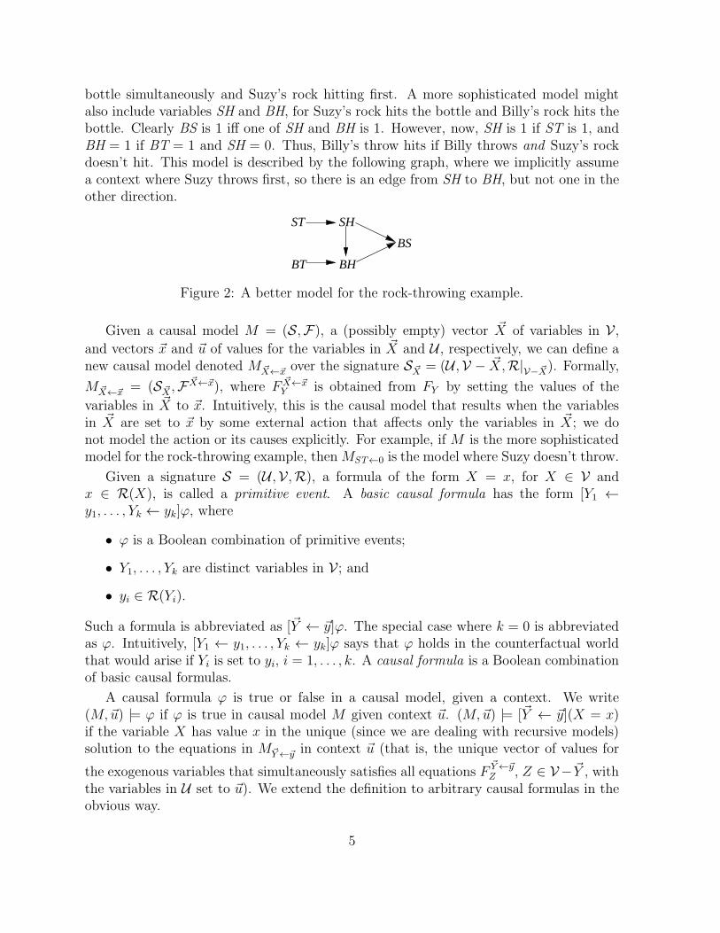
bottle simultaneously and Suzy’s rock hitting first. A more sophisticated model mightalso include variables SH and BH, for Suzy’s rock hits the bottle and Billy’s rock hits thebottle. Clearly BS is 1 iff one of SH and BH is 1. However, now, SH is 1 if ST is 1, andBH = 1 if BT = 1 and SH = 0. Thus, Billy’s throw hits if Billy throws and Suzy’s rockdoesn’t hit. This model is described by the following graph, where we implicitly assumea context where Suzy throws first, so there is an edge from SH to BH, but not one in theother direction.

ST

BT

BS

SH

BH

Figure 2: A better model for the rock-throwing example.

Given a causal model M = (S,F), a (possibly empty) vector ~X of variables in V,

and vectors ~x and ~u of values for the variables in ~X and U , respectively, we can define anew causal model denoted M ~X←~x over the signature S ~X = (U ,V − ~X,R|V− ~X). Formally,

M ~X←~x = (S ~X ,F~X←~x), where F

~X←~xY is obtained from FY by setting the values of the

variables in ~X to ~x. Intuitively, this is the causal model that results when the variablesin ~X are set to ~x by some external action that affects only the variables in ~X; we donot model the action or its causes explicitly. For example, if M is the more sophisticatedmodel for the rock-throwing example, thenMST←0 is the model where Suzy doesn’t throw.

Given a signature S = (U ,V,R), a formula of the form X = x, for X ∈ V andx ∈ R(X), is called a primitive event. A basic causal formula has the form [Y1 ←y1, . . . , Yk ← yk]ϕ, where

• ϕ is a Boolean combination of primitive events;

• Y1, . . . , Yk are distinct variables in V; and

• yi ∈ R(Yi).

Such a formula is abbreviated as [~Y ← ~y]ϕ. The special case where k = 0 is abbreviatedas ϕ. Intuitively, [Y1 ← y1, . . . , Yk ← yk]ϕ says that ϕ holds in the counterfactual worldthat would arise if Yi is set to yi, i = 1, . . . , k. A causal formula is a Boolean combinationof basic causal formulas.

A causal formula ϕ is true or false in a causal model, given a context. We write(M,~u) |= ϕ if ϕ is true in causal model M given context ~u. (M,~u) |= [~Y ← ~y](X = x)if the variable X has value x in the unique (since we are dealing with recursive models)solution to the equations in M~Y←~y in context ~u (that is, the unique vector of values for

the exogenous variables that simultaneously satisfies all equations F~Y←~yZ , Z ∈ V− ~Y , with

the variables in U set to ~u). We extend the definition to arbitrary causal formulas in theobvious way.

5

3 Causality and Responsibility

3.1 Causality

We start with the definition of cause from [Halpern and Pearl 2001a].

Definition 3.1 (Cause) We say that ~X = ~x is a cause of ϕ in (M,~u) if the followingthree conditions hold:

AC1. (M,~u) |= ( ~X = ~x) ∧ ϕ.

AC2. There exist a partition (~Z, ~W ) of V with ~X ⊆ ~Z and some setting (~x′, ~w′) of the

variables in ( ~X, ~W ) such that if (M,~u) |= Z = z∗ for Z ∈ ~Z, then

(a) (M,~u) |= [ ~X ← ~x′, ~W ← ~w′]¬ϕ. That is, changing ( ~X, ~W ) from (~x, ~w) to(~x′, ~w′) changes ϕ from true to false.

(b) (M,~u) |= [ ~X ← ~x, ~W ← ~w′, ~Z ′ ← ~z∗]ϕ for all subsets ~Z ′ of ~Z. That is, setting~W to ~w′ should have no effect on ϕ as long as ~X has the value ~x, even if allthe variables in an arbitrary subset of ~Z are set to their original values in thecontext ~u.

AC3. ( ~X = ~x) is minimal, that is, no subset of ~X satisfies AC2.

AC1 just says that A cannot be a cause of B unless both A and B are true, while AC3is a minimality condition to prevent, for example, Suzy throwing the rock and sneezingfrom being a cause of the bottle shattering. Eiter and Lukasiewicz [2002b] showed thatone consequence of AC3 is that causes can always be taken to be single conjuncts. Thus,from here on in, we talk about X = x being the cause of ϕ, rather than ~X = ~x being thecause. The core of this definition lies in AC2. Informally, the variables in ~Z should bethought of as describing the “active causal process” from X to ϕ. These are the variablesthat mediate between X and ϕ. AC2(a) is reminiscent of the traditional counterfactualcriterion, according to which X = x is a cause of ϕ if change the value of X results in ϕbeing false. However, AC2(a) is more permissive than the traditional criterion; it allowsthe dependence of ϕ on X to be tested under special structural contingencies, in whichthe variables ~W are held constant at some setting ~w′. AC2(b) is an attempt to counteractthe “permissiveness” of AC2(a) with regard to structural contingencies. Essentially, it

ensures that X alone suffices to bring about the change from ϕ to ¬ϕ; setting ~W to ~w′

merely eliminates spurious side effects that tend to mask the action of X .

To understand the role of AC2(b), consider the rock-throwing example again. Inthe model in Figure 1, it is easy to see that both Suzy and Billy are causes of the bottleshattering. Taking ~Z = {ST, BS}, consider the structural contingency where Billy doesn’tthrow (BT = 0). Clearly [ST ← 0,BT← 0]BS = 0 and [ST ← 1,BT← 0]BS = 1 both

6

hold, so Suzy is a cause of the bottle shattering. A symmetric argument shows that Billyis also a cause.

But now consider the model described in Figure 2. It is still the case that Suzy is acause in this model. We can take ~Z = {ST, SH, BS} and again consider the contingencywhere Billy doesn’t throw. However, Billy is not a cause of the bottle shattering. Forsuppose that we now take ~Z = {BT,BH, BS} and consider the contingency where Suzydoesn’t throw. Clearly AC2(a) holds, since if Billy doesn’t throw (under this contingency),

then the bottle doesn’t shatter. However, AC2(b) does not hold. Since BH ∈ ~Z, if we setBH to 0 (it’s original value), then AC2(b) requires that [BT← 1, ST← 0,BH← 0](BS =

1) hold, but it does not. Similar arguments show that no other choice of (~Z, ~W ) makesBilly’s throw a cause.

In [Halpern and Pearl 2001a], a slightly more refined definition of causality is alsoconsidered, where there is a set of allowable settings for the endogenous settings, andthe only contingencies that can be considered in AC2(b) are ones where the settings

( ~W = ~w′, ~X = ~x′) and ( ~W = ~w′, ~X = ~x) are allowable. The intuition here is that we donot want to have causality demonstrated by an “unreasonable” contingency. For example,in the rock throwing example, we may not want to allow a setting where ST = 0, BT = 1,and BH = 0, since this means that Suzy doesn’t throw, Billy does, and yet Billy doesn’t hitthe bottle; this setting contradicts the assumption that Billy’s throw is perfectly accurate.We return to this point later.

3.2 Responsibility

The definition of responsibility in causal models extends the definition of causality.

Definition 3.2 (Degree of Responsibility) The degree of responsibility of X = x forϕ in (M,~u), denoted dr((M,~u), (X = x), ϕ), is 0 if X = x is not a cause of ϕ in (M,~u);

it is 1/(k+ 1) if X = x is a cause of ϕ in (M,~u) and there exists a partition (~Z, ~W ) and

setting (x′, ~w′) for which AC2 holds such that (a) k variables in ~W have different values in

~w′ than they do in the context ~u and (b) there is no partition (~Z ′, ~W ′) and setting (x′′, ~w′′)satisfying AC2 such that only k′ < k variables have different values in ~w′′ than they dothe context ~u.

Intuitively, dr((M,~u), (X = x), ϕ) measures the minimal number of changes that haveto be made in ~u in order to make ϕ counterfactually depend on X . If no partition ofV to (~Z, ~W ) makes ϕ counterfactually depend on (X = x), then the minimal numberof changes in ~u in Definition 3.2 is taken to have cardinality ∞, and thus the degree ofresponsibility of X = x is 0. If ϕ counterfactually depends on X = x, that is, changingthe value of X alone falsifies ϕ in (M,~u), then the degree of responsibility of X = x inϕ is 1. In other cases the degree of responsibility is strictly between 0 and 1. Note thatX = x is a cause of ϕ iff the degree of responsibility of X = x for ϕ is greater than 0.

7

Example 3.3 Consider the voting example from the introduction. Suppose there are 11voters. Voter i is represented by a variable Xi, i = 1, . . . , 11; the outcome is representedby the variable O, which is 1 if Mr. B wins and 0 if Mr. B wins. In the context whereMr. B wins 11–0, it is easy to check that each voter is a cause of the victory (that isXi = 1 is a cause of O = 1, for i = 1, . . . , 11). However, the degree of responsibility ofXi = 1 for is O = 1 is just 1/6, since at least five other voters must change their votesbefore changing Xi to 0 results in O = 0. But now consider the context where Mr. B wins6–5. Again, each voter who votes for Mr. B is a cause of him winning. However, noweach of these voters have degree of responsibility 1. That is, if Xi = 1, changing Xi to 0is already enough to make O = 0; no other variables need to change.

Example 3.4 It is easy to see that Suzy’s throw has degree of responsibility 1/2 for thebottle shattering in the naive model described in Figure 1; Suzy’s throw becomes criticalin the contingency where Billy does not throw. In the “better” model of Figure 2, Suzy’sdegree of responsibility is 1. If we take ~W to consist of {BT,BH}, and keep both variablesat their current setting (that is, consider the contingency where BT = 1 and BH = 0),then Suzy’s throw becomes critical; if she throws, the bottle shatters, and if she does notthrow, the bottle does not shatter (since BH = 0). As we suggested earlier, the setting(ST = 0,BT = 1,BH = 0) may be a somewhat unreasonable one to consider, since itrequires Billy’s throw to miss. If the setting (BH = 1, ST = 0,BH = 0) is not allowable,then we cannot consider this contingency. In that case, Suzy’s degree of responsibility isagain 1/2, since we must consider the contingency where Billy does not throw. Thus, therestriction to allowable settings allows us to capture what seems like a significant intuitionhere.

As we mentioned in the introduction, in a companion paper [Chockler, Halpern, andKupferman 2003] we apply our notion of responsibility to program verification. The ideais to determine the degree of responsibility of the setting of each state for the satisfactionof a specification in a given system. For example, given a specification of the form ✸p(eventually p is true), if p is true in only one state of the verified system, then that statehas degree of responsibility 1 for the specification. On the other hand, if p is true in threestates, each state only has degree of responsibility 1/3. Experience has shown that ifthere are many states with low degree of responsibility for a specification, then either thespecification is incomplete (perhaps p really did have to happen three times, in which casethe specification should have said so), or there is a problem with the system generated bythe program, since it has redundant states.

The degree of responsibility can also be used to provide a measure of the degree offault-tolerance in a system. If a component is critical to an outcome, it will have degree ofresponsibility 1. To ensure fault tolerance, we need to make sure that no component has ahigh degree of responsibility for an outcome. Going back to the example of ✸p, the degreeof responsibility of 1/3 for a state means that the system is robust to the simultaneousfailures of at most two states.

8

3.3 Blame

The definitions of both causality and responsibility assume that the context and thestructural equations are given; there is no uncertainty. We are often interested in assigninga degree of blame to an action. This assignment depends on the epistemic state of theagent before the action was performed. Intuitively, if the agent had no reason to believe,before he performed the action, that his action would result in a particular outcome, thenhe should not be held to blame for the outcome (even if in fact his action caused theoutcome).

There are two significant sources of uncertainty for an agent who is contemplatingperforming an action:

• what the true situation is (that is, what value various variables have); for example,a doctor may be uncertain about whether a patient has high blood pressure.

• how the world works; for example, a doctor may be uncertain about the side effectsof a given medication;

In our framework, the “true situation” is determined by the context; “how the worldworks” is determined by the structural equations. Thus, we model an agent’s uncertaintyby a pair (K,Pr), where K is a set of pairs of the form (M,~u), where M is a causal modeland ~u is a context, and Pr is a probability distribution over K. Following [Halpern andPearl 2001b], who used such epistemic states in the definition of explanation, we call apair (M,~u) a situation.

We think of K as describing the situations that the agent considers possible before Xis set to x. The degree of blame that setting X to x has for ϕ is then the expected degreeof responsibility of X = x for ϕ in (MX←x, ~u), taken over the situations (M,~u) ∈ K. Notethat the situation (MX←x, ~u) for (M,~u) ∈ K are those that the agent considers possibleafter X is set to x.

Definition 3.5 (Blame) The degree of blame of settingX to x for ϕ relative to epistemicstate (K,Pr), denoted db(K,Pr, X ← x, ϕ), is

∑

(M,~u)∈K

dr((MX←x, ~u), X = x, ϕ) Pr((M,~u)).

Example 3.6 Suppose that we are trying to compute the degree of blame of Suzy’sthrowing the rock for the bottle shattering. Suppose that the only causal model thatSuzy considers possible is essentially like that of Figure 2, with some minor modifications:BT can now take on three values, say 0, 1, 2; as before, if BT = 0 then Billy doesn’tthrow, if BT = 1, then Billy does throw, and if BT = 2, then Billy throws extra hard.Assume that the causal model is such that if BT = 1, then Suzy’s rock will hit the bottlefirst, but if BT = 2, they will hit simultaneously. Thus, SH = 1 if ST = 1, and BH = 1 ifBT = 1 and SH = 0 or if BT = 2. Call this structural model M .

At time 0, Suzy considers the following four situations equally likely:

9

• (M,~u1), where ~u1 is such that Billy already threw at time 0 (and hence the bottleis shattered);

• (M,~u2), where the bottle was whole before Suzy’s throw, and Billy throws extrahard, so Billy’s throw and Suzy’s throw hit the bottle simultaneously (this essentiallygives the model in Figure 1);

• (M,~u3), where the bottle was whole before Suzy’s throw, and Suzy’s throw hitbefore Billy’s throw (this essentially gives the model in Figure 2); and

• (M,~u4), where the bottle was whole before Suzy’s throw, and Billy did not throw.

The bottle is already shattered in (M,~u1) before Suzy’s action, so Suzy’s throw is not acause of the bottle shattering, and her degree of responsibility for the shattered bottleis 0. As discussed earlier, the degree of responsibility of Suzy’s throw for the bottleshattering is 1/2 in (M,~u2) and 1 in both (M,~u3) and ((M,~u4). Thus, the degree ofblame is 1

4· 12+ 1

4· 1 + 1

4· 1 = 5

8. If we further require that the contingencies in AC2(b)

involve only allowable settings, and assume that the setting (ST = 0,BT = 1,BH = 0) isnot allowable, then the degree of responsibility of Suzy’s throw in (M,~u3) is 1/2; in thiscase, the degree of blame is 1

4· 12+ 1

4· 12+ 1

4· 1 = 1

2.

Example 3.7 Consider again the example of the firing squad with ten excellent marks-men. Suppose that marksman 1 knows that exactly one marksman has a live bullet in hisrifle, and that all the marksmen will shoot. Thus, he considers 10 augmented situationspossible, depending on who has the bullet. Let pi be his prior probability that marksmani has the live bullet. Then the degree of blame of his shot for the death is pi. The degreeof responsibility is either 1 or 0, depending on whether or not he actually had the livebullet. Thus, it is possible for the degree of responsibility to be 1 and the degree of blameto be 0 (if he mistakenly ascribes probability 0 to his having the live bullet, when in facthe does), and it is possible for the degree of responsibility to be 0 and the degree of blameto be 1 (if he mistakenly ascribes probability 1 to his having the bullet when he in factdoes not).

Example 3.8 The previous example suggests that both degree of blame and degree ofresponsibility may be relevant in a legal setting. Another issue that is relevant in legalsettings is whether to consider actual epistemic state or to consider what the epistemicstate should have been. The former is relevant when considering intent. To see therelevance of the latter, consider a patient who dies as a result of being treated by a doctorwith a particular drug. Assume that the patient died due to the drug’s adverse side effectson people with high blood pressure and, for simplicity, that this was the only cause ofdeath.Suppose that the doctor was not aware of the drug’s adverse side effects. (Formally,this means that he does not consider possible a situation with a causal model where takingthe drug causes death.) Then, relative to the doctor’s actual epistemic state, the doctor’sdegree of blame will be 0. However, a lawyer might argue in court that the doctor should

10

have known that treatment had adverse side effects for patients with high blood pressure(because this is well documented in the literature) and thus should have checked thepatient’s blood pressure. If the doctor had performed this test, he would of course haveknown that the patient had high blood pressure. With respect to the resulting epistemicstate, the doctor’s degree of blame for the death is quite high. Of course, the lawyer’s jobis to convince the court that the latter epistemic state is the appropriate one to considerwhen assigning degree of blame.

Our definition of blame considers the epistemic state of the agent before the action wasperformed. It is also of interest to consider the expected degree of responsibility after theaction was performed. To understand the differences, again consider consider the patientwho dies as a result of being treated by a doctor with a particular drug. The doctor’sepistemic state after the patient’s death is likely to be quite different from her epistemicstate before the patient’s death. She may still consider it possible that the patient died forreasons other than the treatment, but will consider causal structures where the treatmentwas a cause of death more likely. Thus, the doctor will likely have higher degree of blamerelative to her epistemic state after the treatment.

Interestingly, all three epistemic states (the epistemic state that an agent actuallyhas before performing an action, the epistemic state that the agent should have hadbefore performing the action, and the epistemic state after performing the action) havebeen considered relevant to determining responsibility according to different legal theories[Hart and Honore 1985, p. 482].

4 The Complexity of Computing Responsibility and

Blame

In this section we present complexity results for computing the degree of responsibilityand blame for general recursive models.

4.1 The complexity of computing responsibility

Complexity results for computing causality were presented by Eiter and Lukasiewicz[2002a, 2002b]. They showed that the problem of detecting whether X = x is an ac-tual cause of ϕ is ΣP

2 -complete for general recursive models and NP-complete for binarymodels [Eiter and Lukasiewicz 2002b]. (Recall that ΣP

2 is the second level of the poly-nomial hierarchy and that binary models are ones where all random variables can takeon exactly two values.) There is a similar gap between the complexity of computing thedegree of responsibility and blame in general models and in binary models.

For a complexity class A, FPA[logn] consists of all functions that can be computed bya polynomial-time Turing machine with an oracle for a problem in A, which on input

11

x asks a total of O(log |x|) queries (cf. [Papadimitriou 1984]). We show that computing

the degree of responsibility of X = x for ϕ in arbitrary models is FPΣP

2 [logn]-complete.It is shown in [Chockler, Halpern, and Kupferman 2003] that computing the degree ofresponsibility in binary models is FPNP[logn]-complete.

Since there are no known natural FPΣP

2 [logn]-complete problems, the first step in show-ing that computing the degree of responsibility is FPΣP

2 [logn]-complete is to define anFPΣP

2 [logn]-complete problem. We start by defining one that we call MAXQSAT2.

Recall that a quantified Boolean formula [Stockmeyer 1977] (QBF) has the form∀X1∃X2 . . . ψ, where X1, X2, . . . are propositional variables and ψ is a propositional for-mula. A QBF is closed if it has no free propositional variables. TQBF consists of theclosed QBF formulas that are true. For example, ∀X∃Y (X ⇒ Y ) ∈ TQBF. As shownby Stockmeyer [1977], the following problem QSAT2 is ΣP

2 -complete:

QSAT2 = {∃X∀Y ψ(X, Y ) ∈ TQBF : ψ ∈ 3−CNF}.

That is, QSAT2 is the language of all true QBFs of the form ∃ ~X∀~Y ψ, where ψ is a Booleanformula in 3-CNF.

A witness f for a true closed QBF ∃ ~X∀~Y ψ is an assignment f to ~X under which∀~Y ψ is true. We define MAXQSAT2 as the problem of computing the maximal numberof variables in ~X that can be assigned 1 in a witness for ∃ ~X∀~Y ψ. Formally, given a QBFΦ = ∃ ~X∀~Y ψ, define MAXQSAT2(Φ) to be k if there exists a witness for Φ that assigns

exactly k of the variables in ~X the value 1, and every other witness for Φ assigns at mostk′ ≤ k variables in ~X the value 1. If Φ /∈ QSAT2, then MAXQSAT2(Φ) = −1.

Theorem 4.1 MAXQSAT2 is FPΣP

2 [logn]-complete.

Proof: First we prove that MAXQSAT2 is in FPΣP

2 [logn] by describing an algorithm inFPΣP

2 [logn] for solving MAXQSAT2. The algorithm queries an oracle OL for the languageL, defined as follows:

L = {(Φ, k) : k ≥ 0, MAXQSAT2(Φ) ≥ k}.

It is easy to see that L ∈ ΣP2 : if Φ has the form ∃ ~X∀~Y ψ, guess an assignment f that

assigns at least k variables in ~X the value 1 and check whether f is a witness for Φ. Notethat this amounts to checking the validity of ψ with each variable in ~X replaced by itsvalue according to f , so this check is in co-NP, as required. It follows that the languageL is in ΣP

2 . (In fact, it is only a slight variant of QSAT2.) Given Φ, the algorithm forcomputing MAXQSAT2(Φ) first checks if Φ ∈ QSAT2 by making a query with k = 0. Ifit is not, then MAXQSAT2(Φ) is −1. If it is, the algorithm performs a binary search forits value, each time dividing the range of possible values by 2 according to the answer ofOL. The number of possible values of MAXQSAT2(Φ) is then |X|+2 (all values between−1 and |X| are possible), so the algorithm asks OL at most ⌈logn⌉ + 1 queries.

12

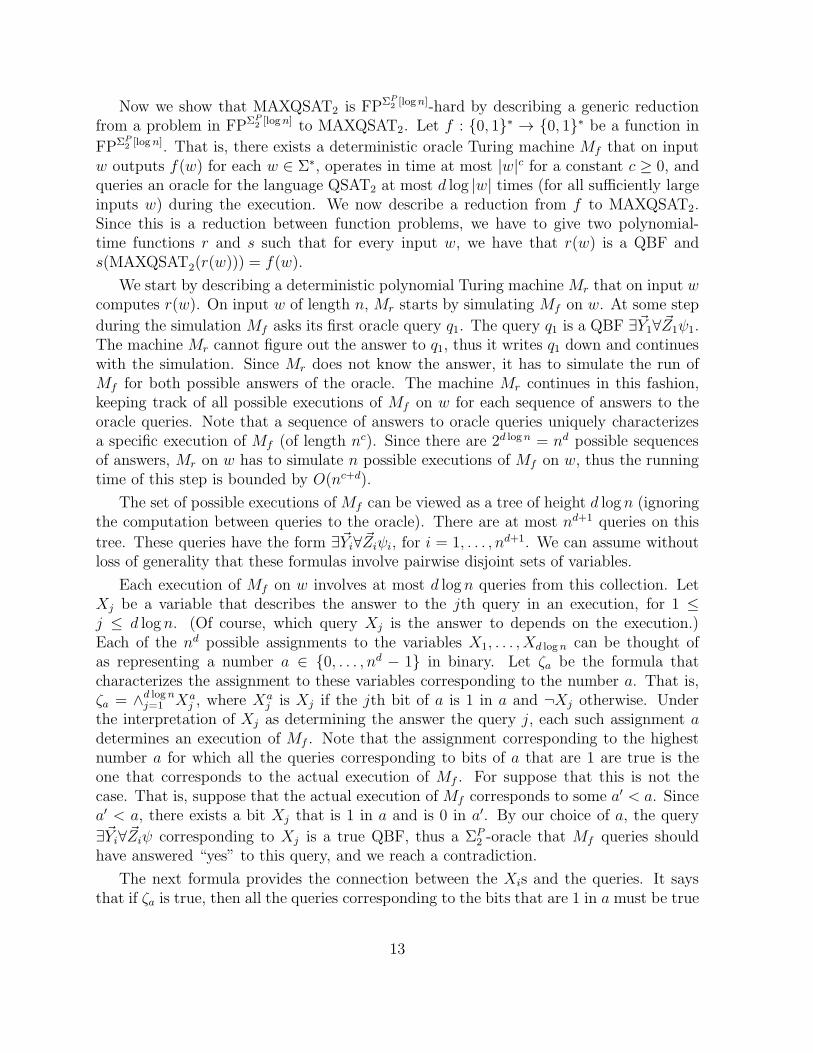
Now we show that MAXQSAT2 is FPΣP

2 [logn]-hard by describing a generic reductionfrom a problem in FPΣP

2 [logn] to MAXQSAT2. Let f : {0, 1}∗ → {0, 1}∗ be a function in

FPΣP

2 [logn]. That is, there exists a deterministic oracle Turing machine Mf that on inputw outputs f(w) for each w ∈ Σ∗, operates in time at most |w|c for a constant c ≥ 0, andqueries an oracle for the language QSAT2 at most d log |w| times (for all sufficiently largeinputs w) during the execution. We now describe a reduction from f to MAXQSAT2.Since this is a reduction between function problems, we have to give two polynomial-time functions r and s such that for every input w, we have that r(w) is a QBF ands(MAXQSAT2(r(w))) = f(w).

We start by describing a deterministic polynomial Turing machineMr that on input wcomputes r(w). On input w of length n, Mr starts by simulating Mf on w. At some step

during the simulation Mf asks its first oracle query q1. The query q1 is a QBF ∃~Y1∀~Z1ψ1.The machine Mr cannot figure out the answer to q1, thus it writes q1 down and continueswith the simulation. Since Mr does not know the answer, it has to simulate the run ofMf for both possible answers of the oracle. The machine Mr continues in this fashion,keeping track of all possible executions of Mf on w for each sequence of answers to theoracle queries. Note that a sequence of answers to oracle queries uniquely characterizesa specific execution of Mf (of length nc). Since there are 2d logn = nd possible sequencesof answers, Mr on w has to simulate n possible executions of Mf on w, thus the runningtime of this step is bounded by O(nc+d).

The set of possible executions ofMf can be viewed as a tree of height d logn (ignoringthe computation between queries to the oracle). There are at most nd+1 queries on this

tree. These queries have the form ∃~Yi∀~Ziψi, for i = 1, . . . , nd+1. We can assume withoutloss of generality that these formulas involve pairwise disjoint sets of variables.

Each execution of Mf on w involves at most d logn queries from this collection. LetXj be a variable that describes the answer to the jth query in an execution, for 1 ≤j ≤ d logn. (Of course, which query Xj is the answer to depends on the execution.)Each of the nd possible assignments to the variables X1, . . . , Xd logn can be thought ofas representing a number a ∈ {0, . . . , nd − 1} in binary. Let ζa be the formula thatcharacterizes the assignment to these variables corresponding to the number a. That is,ζa = ∧d lognj=1 Xa

j , where Xaj is Xj if the jth bit of a is 1 in a and ¬Xj otherwise. Under

the interpretation of Xj as determining the answer the query j, each such assignment adetermines an execution of Mf . Note that the assignment corresponding to the highestnumber a for which all the queries corresponding to bits of a that are 1 are true is theone that corresponds to the actual execution of Mf . For suppose that this is not thecase. That is, suppose that the actual execution of Mf corresponds to some a′ < a. Sincea′ < a, there exists a bit Xj that is 1 in a and is 0 in a′. By our choice of a, the query

∃~Yi∀~Ziψ corresponding to Xj is a true QBF, thus a ΣP2 -oracle that Mf queries should

have answered “yes” to this query, and we reach a contradiction.

The next formula provides the connection between the Xis and the queries. It saysthat if ζa is true, then all the queries corresponding to the bits that are 1 in a must be true

13

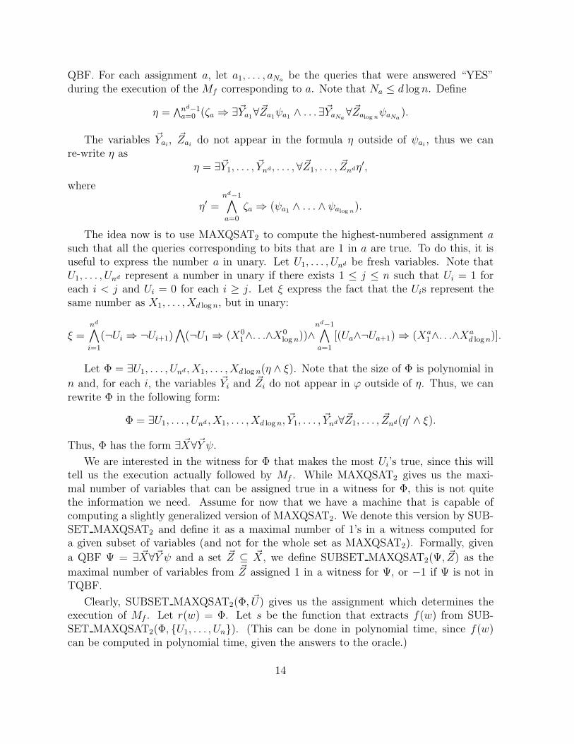
QBF. For each assignment a, let a1, . . . , aNabe the queries that were answered “YES”

during the execution of the Mf corresponding to a. Note that Na ≤ d logn. Define

η =∧nd−1

a=0 (ζa ⇒ ∃~Ya1∀~Za1ψa1 ∧ . . .∃~YaNa∀~Zalog n

ψaNa).

The variables ~Yai,~Zai do not appear in the formula η outside of ψai , thus we can

re-write η asη = ∃~Y1, . . . , ~Ynd, . . . , ∀~Z1, . . . , ~Zndη′,

where

η′ =nd−1∧

a=0

ζa ⇒ (ψa1 ∧ . . . ∧ ψalog n).

The idea now is to use MAXQSAT2 to compute the highest-numbered assignment asuch that all the queries corresponding to bits that are 1 in a are true. To do this, it isuseful to express the number a in unary. Let U1, . . . , Und be fresh variables. Note thatU1, . . . , Und represent a number in unary if there exists 1 ≤ j ≤ n such that Ui = 1 foreach i < j and Ui = 0 for each i ≥ j. Let ξ express the fact that the Uis represent thesame number as X1, . . . , Xd logn, but in unary:

ξ =nd∧

i=1

(¬Ui ⇒ ¬Ui+1)∧(¬U1 ⇒ (X0

1∧. . .∧X0log n))∧

nd−1∧

a=1

[(Ua∧¬Ua+1)⇒ (Xa1∧. . .∧X

ad logn)].

Let Φ = ∃U1, . . . , Und, X1, . . . , Xd logn(η ∧ ξ). Note that the size of Φ is polynomial in

n and, for each i, the variables ~Yi and ~Zi do not appear in ϕ outside of η. Thus, we canrewrite Φ in the following form:

Φ = ∃U1, . . . , Und , X1, . . . , Xd logn, ~Y1, . . . , ~Ynd∀~Z1, . . . , ~Znd(η′ ∧ ξ).

Thus, Φ has the form ∃ ~X∀~Y ψ.

We are interested in the witness for Φ that makes the most Ui’s true, since this willtell us the execution actually followed by Mf . While MAXQSAT2 gives us the maxi-mal number of variables that can be assigned true in a witness for Φ, this is not quitethe information we need. Assume for now that we have a machine that is capable ofcomputing a slightly generalized version of MAXQSAT2. We denote this version by SUB-SET MAXQSAT2 and define it as a maximal number of 1’s in a witness computed fora given subset of variables (and not for the whole set as MAXQSAT2). Formally, given

a QBF Ψ = ∃ ~X∀~Y ψ and a set ~Z ⊆ ~X , we define SUBSET MAXQSAT2(Ψ, ~Z) as the

maximal number of variables from ~Z assigned 1 in a witness for Ψ, or −1 if Ψ is not inTQBF.

Clearly, SUBSET MAXQSAT2(Φ, ~U) gives us the assignment which determines theexecution of Mf . Let r(w) = Φ. Let s be the function that extracts f(w) from SUB-SET MAXQSAT2(Φ, {U1, . . . , Un}). (This can be done in polynomial time, since f(w)can be computed in polynomial time, given the answers to the oracle.)

14

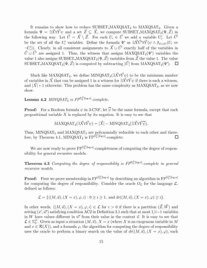
It remains to show how to reduce SUBSET MAXQSAT2 to MAXQSAT2. Given aformula Ψ = ∃ ~X∀~Y ψ and a set ~Z ⊆ ~X , we compute SUBSET MAXQSAT2(Ψ, ~Z) in

the following way. Let ~U = ~X \ ~Z. For each Ui ∈ ~U we add a variable U ′i . Let ~U ′

be the set of all the U ′i variables. Define the formula Ψ′ as ∃ ~X ~U ′∀~Y (ψ ∧∧

Ui∈U(Ui ⇔

¬U ′i)). Clearly, in all consistent assignments to ~X ∪ ~U ′ exactly half of the variables in~U ∪ ~U ′ are assigned 1. Thus, the witness that assigns MAXQSAT2(Ψ

′) variables the

value 1 also assigns SUBSET MAXQSAT2(Ψ, ~Z) variables from ~Z the value 1. The value

SUBSET MAXQSAT2(Ψ, ~Z) is computed by subtracting |~U | from MAXQSAT2(Ψ′).

Much like MAXQSAT2, we define MINQSAT2(∃ ~X∀~Y ψ) to be the minimum number

of variables in ~X that can be assigned 1 in a witness for ∃ ~X∀~Y ψ if there is such a witness,and | ~X|+1 otherwise. This problem has the same complexity as MAXQSAT2, as we nowshow.

Lemma 4.2 MINQSAT2 is FPΣP

2 [logn]-complete.

Proof: For a Boolean formula ψ in 3-CNF, let ψ be the same formula, except that eachpropositional variable X is replaced by its negation. It is easy to see that

MAXQSAT2(∃ ~X∀~Y ψ) = | ~X| −MINQSAT2(∃ ~X∀~Y ψ).

Thus, MINQSAT2 and MAXQSAT2 are polynomially reducible to each other and there-fore, by Theorem 4.1, MINQSAT2 is FPΣP

2 [logn]-complete.

We are now ready to prove FPΣP

2 [logn]-completeness of computing the degree of respon-sibility for general recursive models.

Theorem 4.3 Computing the degree of responsibility is FPΣP

2 [logn]-complete in generalrecursive models.

Proof: First we prove membership in FPΣP

2 [logn] by describing an algorithm in FPΣP

2 [logn]

for computing the degree of responsibility. Consider the oracle OL for the language L,defined as follows:

L = {〈(M,~u), (X = x), ϕ, i〉 : 0 ≥ i ≥ 1, and dr((M,~u), (X = x), ϕ) ≥ i}.

In other words, 〈(M,~u), (X = x), ϕ, i〉 ∈ L for i > 0 if there is a partition (~Z, ~W ) andsetting (x′, ~w′) satisfying condition AC2 in Definition 3.1 such that at most 1/i−1 variablesin W have values different in ~w′ from their value in the context ~u. It is easy to see thatL ∈ ΣP

2 . Given as input a situation (M,~u), X = x (where X is an exogenous variable inMand x ∈ R(X)), and a formula ϕ, the algorithm for computing the degree of responsibilityuses the oracle to perform a binary search on the value of dr((M,~u), (X = x), ϕ), each

15

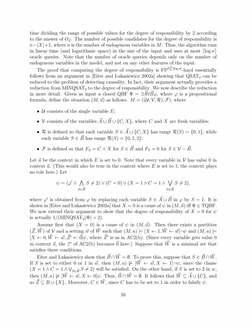
time dividing the range of possible values for the degree of responsibility by 2 accordingto the answer of OL. The number of possible candidates for the degree of responsibility isn−|X|+1, where n is the number of endogenous variables inM . Thus, the algorithm runsin linear time (and logarithmic space) in the size of the input and uses at most ⌈logn⌉oracle queries. Note that the number of oracle queries depends only on the number ofendogenous variables in the model, and not on any other features of the input.

The proof that computing the degree of responsibility is FPΣP

2 [logn]-hard essentiallyfollows from an argument in [Eiter and Lukasiewicz 2002a] showing that QSAT2 can bereduced to the problem of detecting causality. In fact, their argument actually provides areduction from MINQSAT2 to the degree of responsibility. We now describe the reductionin more detail. Given as input a closed QBF Φ = ∃ ~A∀ ~Bϕ, where ϕ is a propositionalformula, define the situation (M,~u) as follows. M = ((U ,V,R),F), where

• U consists of the single variable E;

• V consists of the variables ~A ∪ ~B ∪ {C,X}, where C and X are fresh variables;

• R is defined so that each variable S ∈ ~A ∪ {C,X} has range R(S) = {0, 1}, while

each variable S ∈ ~B has range R(S) = {0, 1, 2};

• F is defined so that FS = C +X for S ∈ ~B and FS = 0 for S ∈ V − ~B.

Let ~u be the context in which E is set to 0. Note that every variable in V has value 0 incontext ~u. (This would also be true in the context where E is set to 1; the context playsno role here.) Let

ψ = (ϕ′ ∧∧

S∈ ~B

S 6= 2) ∨ (C = 0) ∨ (X = 1 ∧ C = 1 ∧∨

S∈ ~B

S 6= 2),

where ϕ′ is obtained from ϕ by replacing each variable S ∈ ~A ∪ ~B in ϕ by S = 1. It isshown in [Eiter and Lukasiewicz 2002a] thatX = 0 is a cause of ψ in (M,~u) iff Φ ∈ TQBF.We now extend their argument to show that the degree of responsibility of X = 0 for ψis actually 1/(MINQSAT2(Φ) + 2).

Assume first that (X = 0) is a cause of ψ in (M,~u). Then there exists a partition

(~Z, ~W ) of V and a setting ~w of ~W such that (M,u) |= [X ← 1, ~W ← ~w]¬ψ and (M,u) |=

[X ← 0, ~W ← ~w, ~Z ′ ← ~0]ψ, where ~Z ′ is as in AC2(b). (Since every variable gets value 0

in context ~u, the ~z∗ of AC2(b) becomes ~0 here.) Suppose that ~W is a minimal set thatsatisfies these conditions.

Eiter and Lukasiewicz show that ~B ∩ ~W = ∅. To prove this, suppose that S ∈ ~B ∩ ~W .If S is set to either 0 or 1 in ~w, then (M,u) 6|= [ ~W ← ~w,X ← 1]¬ψ, since the clause(X = 1 ∧ C = 1 ∧

∨S∈ ~B S 6= 2) will be satisfied. On the other hand, if S is set to 2 in w,

then (M,u) 6|= [ ~W ← ~w,X ← 0]ψ. Thus, ~B ∩ ~W = ∅. It follows that ~W ⊆ ~A ∪ {C}, and

so ~Z ⊆ B ∪ {X}. Moreover, C ∈ ~W , since C has to be set to 1 in order to falsify ψ.

16

Note that every variable in ~W is set to 1 in ~w. This is obvious for C. If there is somevariable S in ~W ∩ ~A that is set to 0 in ~w, we could take S out of ~W while still satisfyingcondition AC2 in Definition 3.1, since every variable S in ~W ∩ ~A has value 0 in context~u and can only be 1 if it is set to 1 in ~w. This contradicts the minimality of W . To showthat Φ ∈ TQBF, consider the truth assignment v that sets a variable S ∈ ~A true iff S isset to 1 in ~W . It suffices to show that v |= ∀ ~Bϕ. Let v′ be any truth assignment that

agrees with v on the variables in ~A. We must show that v′ |= ϕ. Let ~Z ′ consist of all

variables S ∈ ~B such that v′(S) is false. Since (M,u) |= [X ← 0, ~W ← ~1, ~Z ′ ← ~0]ψ, it

follows that (M,u) |= [X ← 0, ~W ← ~1, ~Z ′ ← ~0]ϕ′. It is easy to check that if every variable

in ~W is set to 1, X is set to 0, and ~Z ′ is set to ~0, then every variable in ~A ∪ ~B gets thesame value as it does in v′. Thus, v′ |= ϕ. It follows that Φ ∈ TQBF. This argument also

shows that there is a a witness for Φ (i.e., valuation which makes ∀ ~Bϕ true) that assigns

the value true to all the variables in ~W ∩ ~A, and only to these variables.

Now suppose that if Φ ∈ TQBF and let v be a witness for Φ. Let ~W consist of Ctogether with the variables S ∈ ~A such that v(S) is true. Let ~w set all the variables

in ~W to 1. It is easy to see X = 0 is a cause of ψ, using this choice of ~W and ~wfor AC2. Clearly (M,u) |= [X ← 1, ~W ← ~1]¬ψ, since setting X to 1 and and all

variables in ~W to 1 causes all variables in ~B to have the value 2. On the other hand,(M,u) |= [X ← 0, ~W ← ~1, ~Z ′ ← 0]ψ, since setting X to 0 and ~W ← ~w guarantees that

all variables in ~B have the value 1 and ϕ′ is satisfied. It now follows that a minimal set~W satisfying AC2 consists of C together with a minimal set of variables in ~A that aretrue in a witness for Φ. Thus, | ~W | = MINQSAT2(Φ) + 1, and we have dr((M,~u), (X =

0), ψ) = 1/(| ~W |+ 1) = 1/(MINQSAT2(Φ) + 2).

4.2 The complexity of computing blame

Given an epistemic state (K,Pr), where K consists of N possible augmented situations,each with at most n random variables, the straightforward way to compute db(K,Pr, X ←

x, ϕ) is by computing dr((MX←x,~Y←~y, ~u), X = x, ϕ) for each (M,~u, ~Y ← ~y) ∈ K such that(M,~u) |= X 6= x ∧ ¬ϕ, and then computing the expected degree of responsibility withrespect to these situations, as in Definition 3.5. Recall that the degree of responsibilityin each model M is determined by a binary search, and uses at most ⌈log nM⌉ queriesto the oracle, where nM is the number of endogenous variables in M . Since there are Naugmented situations in K, we get a polynomial time algorithm with

∑Ni=1⌈log ni⌉ oracle

queries. Thus, it is clear that the number of queries is at most the size of the input,and is also at most N⌈log n∗⌉, where n∗ is the maximum number of endogenous variablesthat appear in any of the N augmented situations in K. The type of oracle depends onwhether the models are binary or general. For binary models it is enough to have an NPoracle, whereas for general models we need a ΣP

2 -oracle.

It follows from the discussion above that the problem of computing the degree of blamein general models FPΣP

2 [n], where n is the size of the input. However, the best lower bound

17

we can prove is FPΣP

2 [logn], by reducing the problem of computing responsibility to thatof computing blame; indeed, the degree of responsibility can be viewed as a special caseof the degree of blame with the epistemic state consisting of only one situation. Similarly,lower and upper bounds of FPNP[logn] and FPNP[n] hold for binary models.

An alternative characterization of the complexity of computing blame can be given

by considering the complexity classes FPΣP

2

|| and FPNP|| , which consist of all functions that

can be computed in polynomial time with parallel (i.e., non-adaptive) queries to a ΣP2

(respectively, NP) oracle. (For background on these complexity classes see [Jenner and

Toran 1995; Johnson 1990].) Using FPΣP

2

|| and FPNP|| , we can get matching upper and

lower bounds.

Theorem 4.4 The problem of computing blame in recursive causal models is FPΣP

2

|| -

complete. The problem is FPNP|| -complete in binary causal models.

Proof: As we have observed, the naive algorithm for computing the degree of blameuses N logn∗ queries, where N is the number of augmented situations in the epistemicstate, and n∗ is the maximum number of variables in each one. However, the answersto oracle queries for one situation do not affect the choice of queries for other situations,thus queries for different situations can be asked in parallel. The queries for one situationare adaptive, however, as shown in [Jenner and Toran 1995], a logarithmic number ofadaptive queries can be replaced with a polynomial number of non-adaptive queries byasking all possible combinations of queries in parallel. Thus, the problem of computing

blame is in FPΣP

2

|| for arbitrary recursive models, and in FPNP|| for binary causal models.

For hardness in the case of arbitrary recursive models, we provide a reduction from the

following FPΣP

2

|| -complete problem [Jenner and Toran 1995; Eiter and Lukasiewicz 2002a].

Given N closed QBFs Φ1, . . . ,ΦN , where Φi = ∃ ~Ai∀ ~Biϕi and ϕi is a propositional formulafor 1 ≤ i ≤ N of size O(n), compute the vector (v1, . . . , vN) ∈ {0, 1}

N such that for alli ∈ {1, . . . , N}, we have that vi = 1 iff Φi ∈ TQBF . Without loss of generality, we assume

that all ~Ai’s and ~Bi’s are disjoint. We construct an epistemic state (K,Pr), a formulaϕ, and a variable X such that (v1, . . . , vN ) can be computed in polynomial time fromthe degree of blame of setting X to 1 for ϕ relative to (K,Pr). K consists of the N + 1augmented situations (Mi, ~ui, ∅), i = 1, . . . , N + 1. Each of the models M1, . . . ,MN+1 isof size O(Nn) and involves all the variables that appear in the causal models constructedin the hardness part of the proof of Theorem 4.3, together with fresh random variablesnum1, . . . , numN+1. For 1 ≤ i ≤ N , the equations for the variables in Φi in the situation(Mi, ~ui) at time 1 are the same as in the proof of Theorem 4.3. Thus, Φi ∈ TQBF iffX = 1is a cause of ϕi in (Mi, ~ui) at time 1. In addition, for i = 1, . . . , n, in (Mi, ~ui) at time 1, theequations are such that numi and numN+1 are set to 1 and all other variables (i.e., numj

for j /∈ {i, N1} and all the variables in Φj , j 6= i) are set to 0; at time 0, the equations aresuch that all variables are set to 0. The situation (MN+1, ~uN+1) is such that all variables

18

are set to 0 at both times 0 and 1. Let Pr(Mi, ~ui) = 1/2i(⌈log n⌉) for 1 ≤ i ≤ N , and letPr(MN+1, ~uN+1) = 1− ΣN

i=11/2i(⌈logn⌉). Finally, let ϕ =

∧Ni=1(numi → ϕi) ∧ numN+1.

Clearly ϕ is 0 in all the N + 1 situations at time 0 (since numN+1 is false at time 0in all these situations). At time 1, ϕ is true in (Mi, ~ui), i = 1, . . . , N , iff X = 1 is a causeof ϕi, and ϕ is false in (MN+1, ~uN+1). Thus, the degree of blame db(K,Pr, X ← x, ϕ) isan N⌈log n⌉-bit fraction, where the ith group of bits of size n is not 0 iff Φi ∈ TQBF.It immediately follows that the vector (v1, . . . , vN) can be extracted from db(K,Pr, X ←x, ϕ) by assigning vi the value 1 iff the bits in the ith group in db(K,Pr, X ← x, ϕ) arenot all 0.

We can similarly prove that computing degree of blame in binary models is FPNP|| -hard

by reduction from the problem of determining which of N given propositional formulasof size O(n) are satisfiable. We leave details to the reader.

5 Discussion

We have introduced definition of responsibility and blame, based on Halpern and Pearl’sdefinition of causality. We cannot say that a definition is “right” or “wrong”, but wecan and should examine the how useful a definition is, particularly the extent to which itcaptures our intuitions.

There has been extensive discussion of causality in the philosophy literature, and manyexamples demonstrating the subtlety of the notion. (These examples have mainly beenformulated to show problems with various definitions of causality that have been proposedin the literature.) Thus, one useful strategy for arguing that a definition of causality isuseful is to show that it can handle these examples well. This was in fact done for Halpernand Pearl’s definition of causality (see [Halpern and Pearl 2001a]). While we were not ableto find a corresponding body of examples for responsibility and blame in the philosophyliterature, there is a large body of examples in the legal literature (see, for example, [Hartand Honore 1985]). We plan to do a more careful analysis of how our framework can beused for legal reasoning in future work. For now, we just briefly discuss some relevantissues.

While we believe that “responsibility” and “blame” as we have defined them are impor-tant, distinct notions, the words “responsibility” and “blame” are often used interchange-ably in natural language. It is not always obvious which notion is more appropriate inany given situation. For example, Shafer [2001] says that “a child who pokes at a gun’strigger out of curiosity will not be held culpable for resulting injury or death”. Supposethat a child does in fact poke a gun’s trigger and, as a result, his father dies. According toour definition, the child certainly is a cause of his father’s death (his father’s not leavingthe safety catch on might also be a cause, of course), and has degree of responsibility 1.However, under reasonable assumptions about his epistemic state, the child might wellhave degree of blame 0. So, although we would say that the child is responsible for hisfather’s death, he is not to blame. Shafer talks about the need to take intention into

19

account when assessing culpability. In our definition, we take intention into account tosome extent by considering the agent’s epistemic state. For example, if the child did notconsider it possible that pulling the trigger would result in his father’s death, then surelyhe had no intention of causing his father’s death. However, to really capture intention,we need a more detailed modeled of motivation and preferences.

Shafer [2001] also discusses the probability of assessing responsibility in cases such asthe following.

Example 5.1 Suppose Joe sprays insecticide on his corn field. It is known that sprayinginsecticide increases the probability of catching a cold from 20% to 30%. The cost of acold in terms of pain and lost productivity is $300. Suppose that Joe sprays insecticideand, as a result, Glenn catches a cold. What should Joe pay?

Implicit in the story is a causal model of catching a cold, which is something like thefollowing.2 There are four variables:

• a random variable C (for contact) such that if C = 1 is Glenn is in casual contactwith someone who has a cold, and 0 otherwise.

• a random variable I (for immune) such that if I = 2, Glenn does not catch a coldeven if he both comes in contact with a cold sufferer and lives near a cornfieldsprayed with insecticide; if I = 1, Glenn does not catch a cold even if comes incontact with a cold sufferer, provided he does not live near a cornfield sprayed withinsecticide; and if I = 0, then Glenn catches a cold if he comes in contact with acold sufferer, whether or not he lives near a cornfield sprayed with insecticide;

• a random variable S which is 1 if Glenn lives near a cornfield sprayed with insecticideand 0 otherwise;

• a random variable CC which is 1 if Glenn catches a cold and 0 otherwise.

The causal equations are obvious: CC = 1 iff C = 1 and either I = 0 or I = 1 and S = 1.The numbers suggest that for 70% of the population, I = 2, for 10%, I = 1, and for20%, I = 0. Suppose that no one (including Glenn) knows whether I is 0, 1, or 2. Thus,Glenn’s expected loss from a cold is $60 if Joe does not spray, and $90 if he does. Thedifference of $30 is the economic cost to Glenn of Joe spraying (before we know whetherGlenn actually has a cold).

As Shafer points out, the law does not allow anyone to sue until there has been damage.So consider the situation after Glenn catches a cold. Once Glenn catches a cold, it is clearthat I must be either 0 or 1. Based on the statisical information, I is twice as likely tobe 0 as 1. This leads to an obvious epistemic state, where the causal model where I = 0is assigned probability 2/3 and the causal model where I = 1 is assigned probability 1/3.

2This is not the only reasonable causal model that could correspond to the story, but it is good enoughfor our purposes.

20

In the latter model, Joe’s spraying is not a cause of Glenn’s catching a cold; in the formerit is (and has degree of responsibility 1). Thus, Joe’s degree of blame for the cold is 1/3.This suggests that, once Joe sprays and Glenn catches a cold, the economic damage is$100.

This example also emphasizes the importance of distinguishing between the epistemicstates before and after the action is taken, an issue already discussed in Section 3.3.Indeed, examining the situation after Glenn caught cold enables us to ascribe probability0 to the situation where Glenn is immune, and thus increases Joe’s degree of blame forGlenn’s cold.

Example 5.1 is a relatively easy one, since the degree of responsibility is 1. Things canquickly get more complicated. Indeed, a great deal of legal theory is devoted to issues ofresponsibility (the classic reference is [Hart and Honore 1985]). There are a number ofdifferent legal principles that are applied in determining degree of responsibility; some ofthese occasionally conflict (at least, they appear to conflict to a layman!). For example,in some cases, legal practice (at least, American legal practice) does not really considerdegree of responsibility as we have defined it. Consider the rock throwing example, andsuppose the bottle belongs to Ned and is somewhat valuable; in fact, it is worth $100.

• Suppose both Suzy and Billy’s rock hit the bottle simultaneously, and all it takes isone rock to shatter the bottle. Then they are both responsible for the shattering todegree 1/2 (and both have degree of blame 1/2 if this model is commonly known).Should both have to pay $50? What if they bear different degrees of responsibility?

Interestingly, a standard legal principle is also that “an individual defendant’s re-sponsibility does not decrease just because another wrongdoer was also an actualand proximate cause of the injury” (see [Public Trust 2003]). That is, our notion ofhaving a degree of responsibility less than one is considered inappropriate in somecases in standard tort law, as is the notion of different degrees of responsibility. Notethat if Billy is broke and Suzy can afford $100, the doctrine of joint and several li-ability, also a standard principle in American tort law, rules that Ned can recoverthe full $100 from Suzy.

• Suppose that instead it requires two rocks to shatter the bottle. Should that case betreated any differently? (Recall that, in this case, both Suzy and Billy have degreeof responsibility 1.)

• If Suzy’s rock hits first and it requires only one rock to shatter the bottle then, as wehave seen, Suzy has degree of responsibility 0 or 1/2 (depending on whether we con-sider only allowable settings) and Billy has degree of responsibility 0. Nevertheless,standard legal practice would probably judge Billy (in part) responsible.

In some cases, it seems that legal doctrine confounds what we have called cause, blame,and responsibility. To take just one example from Hart and Honoree [1985, p. 74], assume

21

that A throws a lighted cigarette into the bracken near a forest and a fire starts. Just asthe fire is about to go out, B deliberately pours oil on the flame. The fire spreads andburns down the forest. Clearly B’s action was a cause of the forest fire. Was A’s actionalso a cause of the forest fire? According to Hart and Honore, he is not, whether or nothe intended to cause the fire; only B was. In our framework, it depends on the causalmodel. If B would have started a fire anyway, whether or not A’s fire went out, then A isindeed not the cause; if B would not have started a fire had he not seen A’s fire, then A isa cause (as is B), although is degree of resonsibility for the fire is only 1/2. Furthermore,A’s degree of blame may be quite low. Our framework lets us make distinctions here thatseem to be relevant for legal reasoning.

While these examples show that legal reasoning treats responsibility and blame some-what differently from the way we do, we believe that a formal analysis of legal reasoningusing our definitions would be helpful, both in terms of clarifying the applicability of ourdefinitions and in terms of clarifying the basis for various legal judgments. As we said,we hope to focus more on legal issues in future work.

Our notion of degree of responsibility focuses on when an action becomes critical.Perhaps it may have been better termed a notion of “degree of criticality”. While webelieve that it is a useful notion, there are cases where a more refined notion may beuseful. For example, consider a voter who voted for Mr. B in the case of a 1-0 vote and avoter who voted for Mr. B in the case of a 100-99 vote. In both case, that voter has degreeof responsibility 1. While it is true that, in both cases, that voter’s vote was critical, inthe second case, the voter may believe that his responsibility is more diffuse. We oftenhere statements like “Don’t just blame me; I wasn’t the only one who voted for him!” Thesecond author is current working with I. Gilboa on a definition of resonsibility that usesthe game-theoretic notion of Shapley value (see, for example, [Osborne and Rubinstein1994]) to try to distinguish these examples.

As another example, suppose that one person dumps 900 pounds of garbage on aporch and another dumps 100 pounds. The porch can only bear 999 pounds of load, so itcollapses. Both people here have degree of responsibility 1/2 according to our definition,but there is an intuition that suggests that the person who dumped 900 pounds shouldbear greater responsibliity. We can easily accommodate this in our framework by puttingweights on variables. If we use wt(X) to denote the weight of a X and wt( ~W ) to denote the

sum of the weights of variables in the set ~W , then we can define the degree of responsibilityof X = x for ϕ to be wt(X)/(wt( ~W ) + wt(X), where ~W is a set of minimal weight forwhich AC2 holds. This definition agrees with the one we use if the weights of all variablesare 1, so this can be viewed as a generalization of our current definition.

These examples show that there is much more to be done in clarifying our understand-ing of responsibility and blame. Because these notions are so central in law and morality,we believe that doing so is quite worthwhile.

22

Acknowledgment We thank Michael Ben-Or and Orna Kupferman for helpful dis-cussions. We particularly thank Chris Hitchcock, who suggested a simplification of thedefinition of blame and pointed out a number of typos and other problems in an earlierversion of the paper.

References

Chockler, H., J. Y. Halpern, and O. Kupferman (2003). What causes asystem to satisfy a specification? Unpublished manuscript. Available athttp://www.cs.cornell.edu/home/halpern/papers/resp.ps.

Collins, J., N. Hall, and L. A. Paul (Eds.) (2003). Causation and Counterfactuals.Cambridge, Mass.: MIT Press.

Eiter, T. and T. Lukasiewicz (2002a). Causes and explanations in the structural-modelapproach: tractable cases. In Proc. Eighteenth Conference on Uncertainty in Arti-ficial Intelligence (UAI 2002), pp. 146–153.

Eiter, T. and T. Lukasiewicz (2002b). Complexity results for structure-based causality.Artificial Intelligence 142 (1), 53–89.

Hall, N. (2003). Two concepts of causation. In J. Collins, N. Hall, and L. A. Paul (Eds.),Causation and Counterfactuals. Cambridge, Mass.: MIT Press.

Halpern, J. Y. and J. Pearl (2001a). Causes and explanations: A structural-model ap-proach. Part I: Causes. In Proc. Seventeenth Conference on Uncertainty in ArtificialIntelligence (UAI 2001), pp. 194–202. The full version of the paper is available athttp://www.cs.cornell.edu/home/halpern.

Halpern, J. Y. and J. Pearl (2001b). Causes and explanations: A structural-model ap-proach. Part II: Explanations. In Proc. Seventeenth International Joint Conferenceon Artificial Intelligence (IJCAI ’01), pp. 27–34. The full version of the paper isavailable at http://www.cs.cornell.edu/home/halpern.

Hart, H. L. A. and T. Honore (1985). Causation in the Law (Second Edition ed.).Oxford, U.K.: Oxford University Press.

Hume, D. (1739). A Treatise of Human Nature. London: John Noon.

Jenner, B. and J. Toran (1995). Computing functions with parallel queries to NP.Theoretical Computer Science 141, 175–193.

Johnson, D. (1990). A catalog of complexity classes. In J. van Leeuwen (Ed.), Handbookof Theoretical Computer Science, Volume A, Chapter 2. Elsevier Science.

Osborne, M. J. and A. Rubinstein (1994). A Course in Game Theory. Cambridge,Mass.: MIT Press.

Papadimitriou, C. H. (1984). The complexity of unique solutions. Journal of ACM 31,492–500.

23

Pearl, J. (2000). Causality: Models, Reasoning, and Inference. New York: CambridgeUniversity Press.

Public Trust (2003). Tort law issues/fact sheets.http://www.citizen.org/congress/civjus/tort/tortlaw/articles.cfm?ID=834).

Shafer, G. (1996). The Art of Causal Conjecture. Cambridge, Mass.: MIT Press.

Shafer, G. (2001). Causality and responsibility. Cardozo Law Review 22, 101–123.

Stockmeyer, L. J. (1977). The polynomial-time hierarchy. Theoretical Computer Sci-ence 3, 1–22.

Zimmerman, M. (1988). An Essay on Moral Responsibility. Totowa, N.J.: Rowman andLittlefield.

24